The Application of Complex Seismic Attributes in Thin Bed

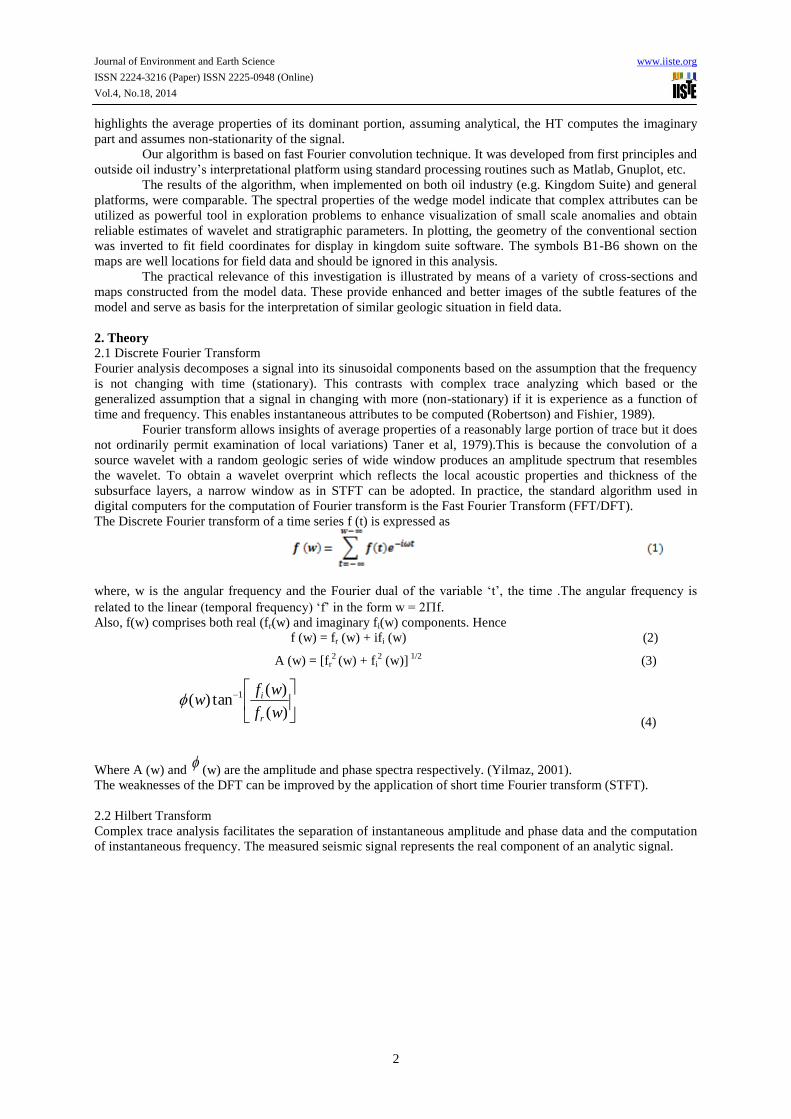
Journal of Environment and Earth Science www.iiste.org

ISSN 2224-3216 (Paper) ISSN 2225-0948 (Online)

Vol.4, No.18, 2014

1

The Application of Complex Seismic Attributes in Thin Bed

Reservoir Analysis

Williams Ofuyah 1*

Olatunbosun Alao 2 Moses Olorunniwo

2

1.Department of Earth Sciences, Federal University of Petroleum Resources, Effurun, Nigeria

2.Department of Geology, Obafemi Awolowo University, Ile-Ife, Nigeria

* E-mail of the corresponding author: [email protected]

Abstract

Geologic models of hydrocarbon reservoirs facilitate enhanced visualization, volumetric calculation, well

planning and prediction of migration path for fluid. In order to obtain new insights and test the mappability of a

geologic feature, spectral decomposition techniques i.e. Discrete Fourier Transform (DFT), Short-Time Fourier

Transform (STFT), Maximum Entropy, Hilbert Transform (HT), etc. can be employed. This paper presents the

results of the application of DFT and HT to a two dimensional, 50Hz low impedance wedge model, representing

typical geologic environment around a prospective hydrocarbon zone. While the DFT represents the frequency

and phase spectra of a signal, assumes stationarity and highlights the average properties of its dominant portion,

assuming analytical, the HT computes the imaginary part and assumes non-stationarity of the signal. Our

algorithm is based on fast Fourier convolution technique. It was developed from first principles and outside oil

industry’s interpretational platform using standard processing routines such as Matlab, Gnuplot, programs. The

results of the algorithm, when implemented on both oil industry (e.g. Kingdom Suite) and general platforms,

were comparable. The spectral properties of the wedge model indicate that complex attributes can be utilized as

powerful tool in exploration problems to enhance visualization of small scale anomalies and obtain reliable

estimates of wavelet and stratigraphic parameters. The practical relevance of this investigation is illustrated by

means of cross-sections and maps constructed from the model data. These provide enhanced images of the subtle

features of the model and serve as basis for the interpretation of similar geologic situations in field data.

Keywords: Discrete Fourier transform, Hilbert transform, Maximum Entropy, Short time Fourier transform,

Spectral decomposition

1. Introduction

Hydrocarbon habitats of the geological provinces of the world are associated with structure and stratigraphy

found in sedimentary basins, extensional provinces, compression1 provinces and strike-slip regimes. These

habitats (high impedance, low impedance, clean and unclean formations) are characterized by linear

displacement of rock forms or faults.

The faults constitute traps, which, in turn, become reservoir rocks when fluids arising from chemical

decomposition of organic matter at depth (source rock) are impeded from further movement by a barrier (cap

rock) after accumulation. The nature of the reservoir rock formed is dependent on the play fairways and

hydrocarbon systems of the geological province concerned.

The reservoir are, on the basis of scale, classified as structural (Anticline, Syncline, Mega-Fault, etc.) or

stratigraphic (Wedge or Pinch-out, Channel, Reef, Micro-Fault, etc.) or a combination of the two (Tarbuck and

Lutgens, 1990).

The high incidence of subtle trap accumulations in hydrocarbon province has led to the need for a high

resolution interpretation scheme such as spectral decomposition of model data to facilitate the identification and

characterization of these features. The variations of signal amplitude such as abrupt, gradual and subtle or gentle,

are generally among the most meaningful features for extracting the information content of signal. The

discontinuities of image intensity for instance, indicate the contours of the different objects constituting the

image. If the signal has structures that are assumed to belong to different scales, its information content can be

sorted into a set of elementary blocks of varying sizes, and can be delayed or fast tracked.

Seismic interpretation objectives include enhanced resolution improved visualization of structural and

particularly stratigraphic features, thickness estimation for thin-bed reservoir, noise filtering or suppression,

direct hydrocarbon indication, etc.

Geologic models of hydrocarbon reservoirs facilitate enhanced visualization, volumetric calculation,

well planning and prediction of fluid flow and direction. In order to obtain new insights and test the mappability

of a geologic feature, spectral decomposition techniques i.e. Discrete Fourier Transform (DFT), Short-Time

Fourier Transform (STFT), Maximum Entropy, Hilbert Transform (HT), etc. can be employed.

This paper presents the results of the application of DFT and HT to a two dimensional, 50Hz low impedance

wedge model, about 50 milliseconds thick, representing typical geologic environment around a prospective

hydrocarbon zone.

While the DFT represents the frequency and phase spectra of a signal, assumes stationarity and

http://www.iiste.org/

mailto:[email protected]



Vol.4, No.18, 2014

2

highlights the average properties of its dominant portion, assuming analytical, the HT computes the imaginary

part and assumes non-stationarity of the signal.

Our algorithm is based on fast Fourier convolution technique. It was developed from first principles and

outside oil industry’s interpretational platform using standard processing routines such as Matlab, Gnuplot, etc.

The results of the algorithm, when implemented on both oil industry (e.g. Kingdom Suite) and general

platforms, were comparable. The spectral properties of the wedge model indicate that complex attributes can be

utilized as powerful tool in exploration problems to enhance visualization of small scale anomalies and obtain

reliable estimates of wavelet and stratigraphic parameters. In plotting, the geometry of the conventional section

was inverted to fit field coordinates for display in kingdom suite software. The symbols B1-B6 shown on the

maps are well locations for field data and should be ignored in this analysis.

The practical relevance of this investigation is illustrated by means of a variety of cross-sections and

maps constructed from the model data. These provide enhanced and better images of the subtle features of the

model and serve as basis for the interpretation of similar geologic situation in field data.

2. Theory

2.1 Discrete Fourier Transform

Fourier analysis decomposes a signal into its sinusoidal components based on the assumption that the frequency

is not changing with time (stationary). This contrasts with complex trace analyzing which based or the

generalized assumption that a signal in changing with more (non-stationary) if it is experience as a function of

time and frequency. This enables instantaneous attributes to be computed (Robertson) and Fishier, 1989).

Fourier transform allows insights of average properties of a reasonably large portion of trace but it does

not ordinarily permit examination of local variations) Taner et al, 1979).This is because the convolution of a

source wavelet with a random geologic series of wide window produces an amplitude spectrum that resembles

the wavelet. To obtain a wavelet overprint which reflects the local acoustic properties and thickness of the

subsurface layers, a narrow window as in STFT can be adopted. In practice, the standard algorithm used in

digital computers for the computation of Fourier transform is the Fast Fourier Transform (FFT/DFT).

The Discrete Fourier transform of a time series f (t) is expressed as

where, w is the angular frequency and the Fourier dual of the variable ‘t’, the time .The angular frequency is

related to the linear (temporal frequency) ‘f’ in the form w = 2f.

Also, f(w) comprises both real (fr(w) and imaginary fi(w) components. Hence

f (w) = fr (w) + ifi (w) (2)

A (w) = [fr2 (w) + fi

2 (w)]

1/2 (3)

)(

)(tan)( 1

wf

wfw

r

i

(4)

Where A (w) and

(w) are the amplitude and phase spectra respectively. (Yilmaz, 2001).

The weaknesses of the DFT can be improved by the application of short time Fourier transform (STFT).

2.2 Hilbert Transform

Complex trace analysis facilitates the separation of instantaneous amplitude and phase data and the computation

of instantaneous frequency. The measured seismic signal represents the real component of an analytic signal.




Vol.4, No.18, 2014

3

Figure 1. Complex Trace: Isometric diagram of portion of an actual seismic trace.

(After Taner et al, 1979).

The Hilbert transformation is a filtering operation that passes the amplitudes of the spectral components

unchanged but alters their phases by the ninety degrees. Using the notation above, in equation (2), fi (w) is the

Hilbert transform of fr (w) (Dobrin, 1988). The complex trace derivatives are instantaneous amplitude (envelope

or reflection strength), instantaneous phase and instantaneous frequency and have expressions similar to the

Fourier derivatives.

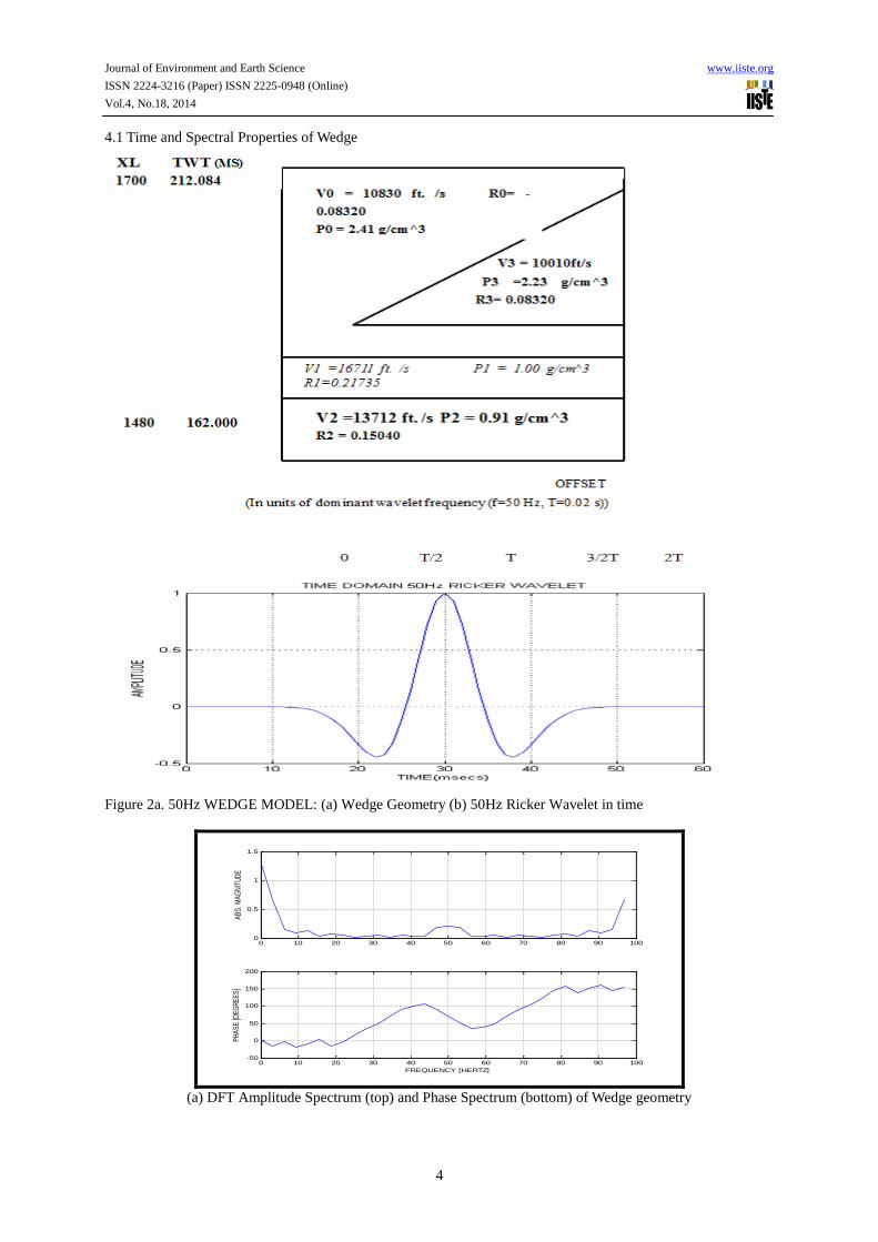
3. Spectral Decomposition of Wedge Model We computed the frequency attributes of a thinning bed reservoir model, a low impedance wedge. The wedge

represents lateral variations in lithofacies and was examined with a 50 Hz using the fast Fourier transform (FFT)

convolution technique. The Ricker wavelet was convolved with a four-layer reflectivity series, where the third

layer is the thin bed. The geometry, seismic parameters, time and frequency characteristics of the model

including the top and base surfaces of the wedge are shown in figure 2a and 2b.In addition, its conventional

section, amplitude, phase and frequency maps highlighting tuning effects are presented in figures 3. The

effective offset in figure 2(a) is 0 to 2T, where T represents period. The acoustic velocity values used are 10,010

ft/s inside the wedge and 10,830 ft/s outside the wedge showing that the thinning bed, about 50 ms thick, is a low

impedance layer. The computed mode (figure 3) is noise free..The Thickness of the wedge is denoted in units of

the dominant (center) period corresponding to the dominant frequency of the Ricker wavelet (zero-phase) used in

modeling. The center frequency used for simulation in this evaluation is 50Hz implying a period of 20

milliseconds. The spectral properties of the model indicate that att thick locations of the wedge, the central peaks

of the corresponding reflections mark the top and bottom. The reflections interfere with each other as the wedge

thins, giving weak resolution of the top and bottom surfaces of the wedge below about a quarter period.

4. Results and Interpretation

In seismic attribute analysis, amplitude or magnitude indicates local concentration of energy; phase measures

discontinuity or faulting, while the frequency attribute reflects attenuation spots and may indicate hydrocarbon

presence.




Vol.4, No.18, 2014

4

4.1 Time and Spectral Properties of Wedge

Figure 2a. 50Hz WEDGE MODEL: (a) Wedge Geometry (b) 50Hz Ricker Wavelet in time

0 10 20 30 40 50 60 70 80 90 1000

0.5

1

1.5

AB

S. M

AG

NIT

UD

E

0 10 20 30 40 50 60 70 80 90 100-50

0

50

100

150

200

PH

AS

E [D

EG

RE

ES

]

FREQUENCY [HERTZ]

(a) DFT Amplitude Spectrum (top) and Phase Spectrum (bottom) of Wedge geometry




Vol.4, No.18, 2014

5

0 10 20 30 40 50 60 70 80 900

0.1

0.2

0.3

0.4

0.5

AB

S. M

AG

NIT

UD

E

0 10 20 30 40 50 60 70 80 900

50

100

150

200P

HA

SE

[DE

GR

EE

S]

FREQUENCY [HERTZ]

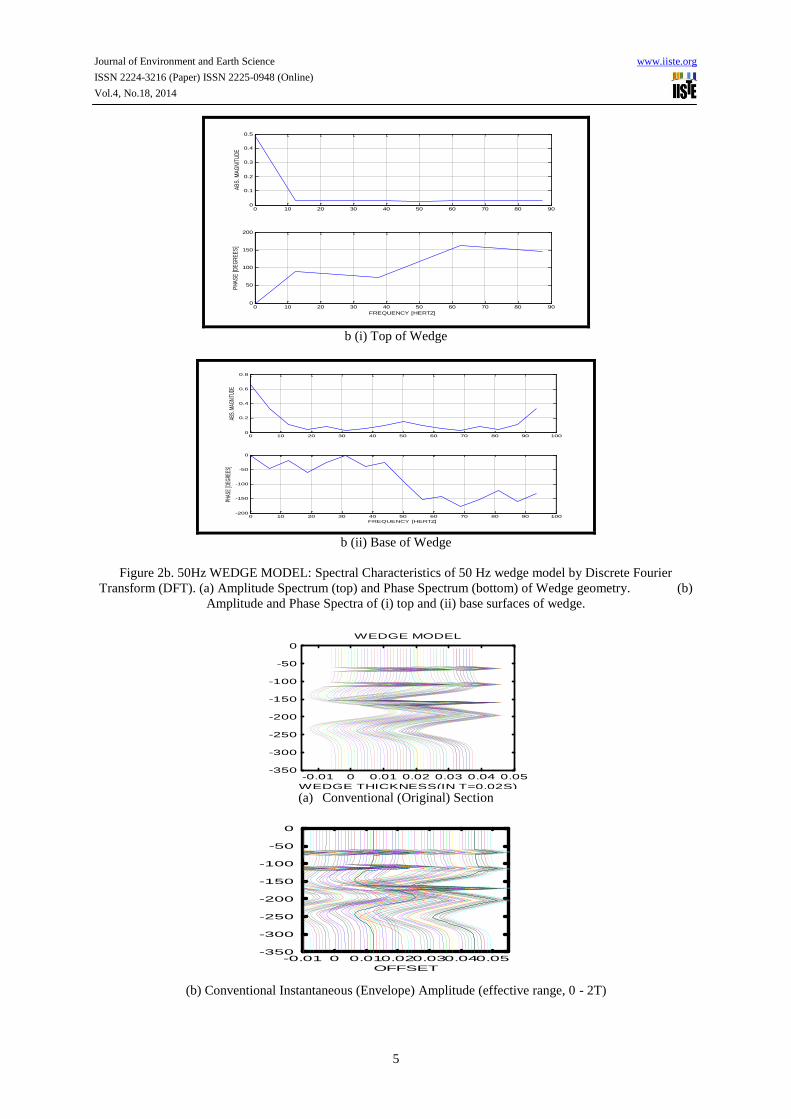
b (i) Top of Wedge

0 10 20 30 40 50 60 70 80 90 1000

0.2

0.4

0.6

0.8

ABS.

MAG

NITU

DE

0 10 20 30 40 50 60 70 80 90 100-200

-150

-100

-50

0

PHAS

E [D

EGRE

ES]

FREQUENCY [HERTZ]

b (ii) Base of Wedge

Figure 2b. 50Hz WEDGE MODEL: Spectral Characteristics of 50 Hz wedge model by Discrete Fourier

Transform (DFT). (a) Amplitude Spectrum (top) and Phase Spectrum (bottom) of Wedge geometry. (b)

Amplitude and Phase Spectra of (i) top and (ii) base surfaces of wedge.

-350

-300

-250

-200

-150

-100

-50

0

-0.01 0 0.01 0.02 0.03 0.04 0.05

TWO-

WAY

TIME

(MSE

CS)

WEDGE THICKNESS(IN T=0.02S)

WEDGE MODEL

(a) Conventional (Original) Section

(b) Conventional Instantaneous (Envelope) Amplitude (effective range, 0 - 2T)

-350

-300

-250

-200

-150

-100

-50

0

-0.01 0 0.010.020.030.040.05

TWO

-WAY

TIM

E (m

SECS

)

OFFSET

INSTANTANEOUS AMPLITUDE




Vol.4, No.18, 2014

6

(c)Kingdom suite of (a)

(d) HT Envelope Amplitude of (a)

Figure 3. 50Hz WEDGE MODEL: (a) Conventional (Original) Section (b) Conventional Instantaneous

(Envelope) Amplitude (effective range, 0 - 2T) (c) Kingdom suite display of Conventional Section in (a), (d) HT

Instantaneous (Envelope) Amplitude of (a).




Vol.4, No.18, 2014

7

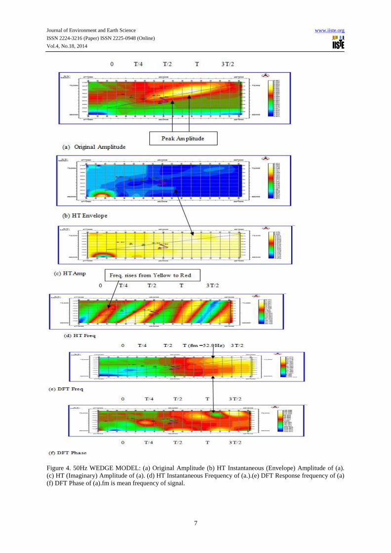
Figure 4. 50Hz WEDGE MODEL: (a) Original Amplitude (b) HT Instantaneous (Envelope) Amplitude of (a).

(c) HT (Imaginary) Amplitude of (a). (d) HT Instantaneous Frequency of (a.).(e) DFT Response frequency of (a)

(f) DFT Phase of (a).fm is mean frequency of signal.




Vol.4, No.18, 2014

8

4.2 Instantaneous (Envelope) Amplitude

As shown in fig 3, there is high amplitude at about half period i.e amplitude tuning .The amplitude falls as the

bed thins to zero thickness as a result of destructive interference.

4.3 Phase

The phase attributes measure coherency and dip of reflection. The response phase (fig. 4f) sections show the

continuity of the wedge and reflect average phase values which dip to approximately 20 degrees at less than T/4

and about 3T/2 thicknesses. The values oscillate about zero at other thickness values. .This phenomenon is

explained in Widess (1973).

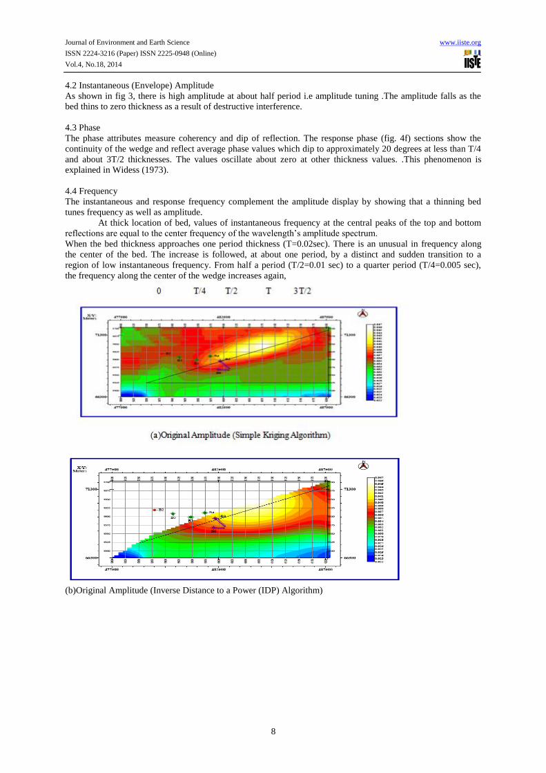
4.4 Frequency

The instantaneous and response frequency complement the amplitude display by showing that a thinning bed

tunes frequency as well as amplitude.

At thick location of bed, values of instantaneous frequency at the central peaks of the top and bottom

reflections are equal to the center frequency of the wavelength’s amplitude spectrum.

When the bed thickness approaches one period thickness (T=0.02sec). There is an unusual in frequency along

the center of the bed. The increase is followed, at about one period, by a distinct and sudden transition to a

region of low instantaneous frequency. From half a period (T/2=0.01 sec) to a quarter period (T/4=0.005 sec),

the frequency along the center of the wedge increases again,

(b)Original Amplitude (Inverse Distance to a Power (IDP) Algorithm)




Vol.4, No.18, 2014

9

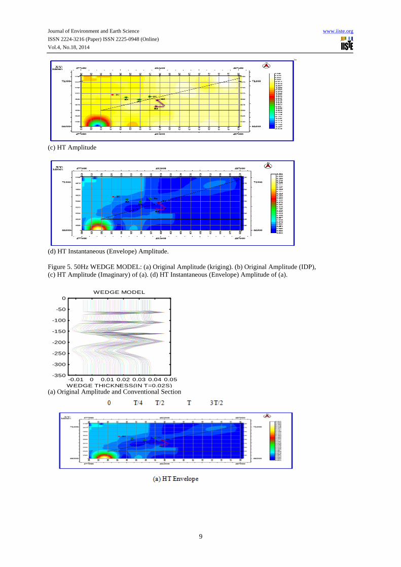
(c) HT Amplitude

(d) HT Instantaneous (Envelope) Amplitude.

Figure 5. 50Hz WEDGE MODEL: (a) Original Amplitude (kriging). (b) Original Amplitude (IDP),

(c) HT Amplitude (Imaginary) of (a). (d) HT Instantaneous (Envelope) Amplitude of (a).

-350

-300

-250

-200

-150

-100

-50

0

-0.01 0 0.01 0.02 0.03 0.04 0.05

TWO

-WAY

TIM

E(M

SECS

)

WEDGE THICKNESS(IN T=0.02S)

WEDGE MODEL

(a) Original Amplitude and Conventional Section




Vol.4, No.18, 2014

10

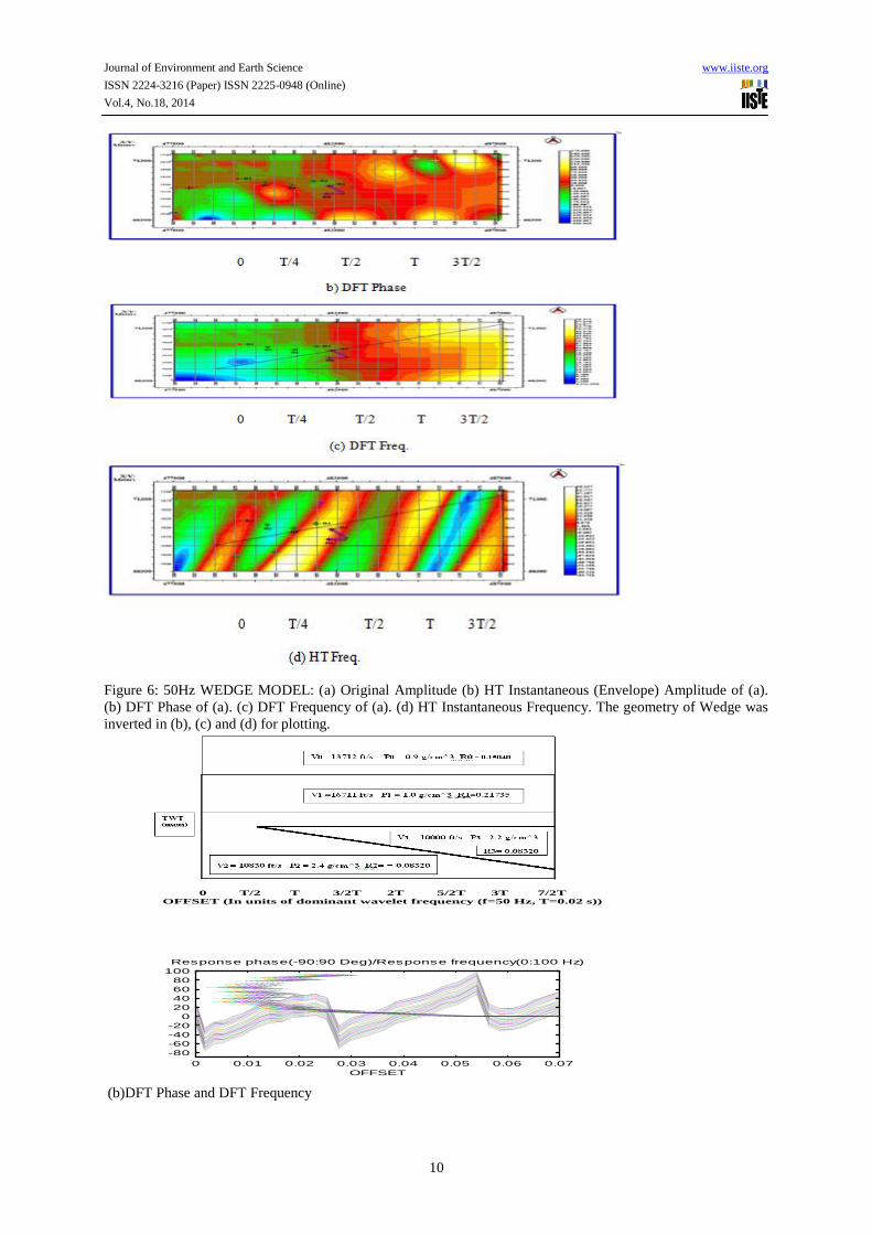
Figure 6: 50Hz WEDGE MODEL: (a) Original Amplitude (b) HT Instantaneous (Envelope) Amplitude of (a).

(b) DFT Phase of (a). (c) DFT Frequency of (a). (d) HT Instantaneous Frequency. The geometry of Wedge was

inverted in (b), (c) and (d) for plotting.

0 T/2 T 3/2T 2T 5/2T 3T 7/2T

OFFSET (In units of dominant wavelet frequency (f=50 Hz, T=0.02 s))

-80

-60

-40

-20

0

20

40

60

80

100

0 0.01 0.02 0.03 0.04 0.05 0.06 0.07Resp

onse

phas

e(De

g)/fre

q.(Hz

)

OFFSET

Response phase(-90:90 Deg)/Response frequency(0:100 Hz)

(b)DFT Phase and DFT Frequency




Vol.4, No.18, 2014

11

-200

-150

-100

-50

0

50

100

150

200

0 0.01 0.02 0.03 0.04 0.05 0.06 0.07 0.08

IN

S.

PH

AS

E(

-1

80

:1

80

De

g)

/F

RE

.(

-1

50

:1

50

Hz

)

OFFSET (WEDGE T HICKNESS)

INST ANT .PHASE(-180:180Deg)/FREQ.(RED,GREEN)(-150:150Hz)

(c)HT Instantaneous Phase and Instantaneous frequency

Figure 7. 50Hz WEDGE MODEL: (a) Wedge Geometry (b) Combined plots of DFT Phase and Frequency (c)

Combined plots of HT Instantaneous Phase and Instantaneous frequency.

An abnormally high region reappears when the bed becomes less than a quarter (T<0.005 sec) period

thick because the thin bed medium delineates the wavelet and increases the mean frequency of the resultant

reflection with respect to the basic wavelet

The frequency pattern is quite conspicuous. The combination of the instantaneous amplitude and

frequency sections can therefore be used with field data to obtain a more detailed interpretation of a thinning bed.

This includes reliable thickness estimation in seismic stratigraphy. Higher resolutions in the region below a half

period, difficult to interpret on the standard section, could be obtained.

The composite reflection which delineates each of the lithofacies is the superposition of individual

reflections and it changes with thickness. It has been established (Taner et al 1979) that variations as pinch-outs

and the edges of hydrocarbon-water interfaces tend to change instantaneous frequency rapidly .This

phenomenon occurs at thickness of T/4 of the wedge . Regions of frequency fall are associated with layers below

hydrocarbon zones.

We deduce the following from figures 5 and 6

(a) At T/2 (λ/4 tuning point), maximum amplitude (yellow) occurs due to constructive interference. But

destructive interference occurs as the bed thins (Green).

(b) In fig. 6b, DFT phase changes to 900, between T and T/2 indicating bed thinning

(c) Fig.6c shows Nyquist amplitude (light blue). This indicates point of symmetry, corresponding to the

maximum useful frequency in the wavelet used.

(d) At thick location of the thin bed, DFT phase is nearly equal to 0o or 180

o, when normalized and the DFT

frequency gives the mean frequency (52.9Hz) of the spectrum of the 50Hz Ricker wavelength.

(e) In In fig. 6c, d and fig 7, DFT frequency and HT Instantaneous frequency maps, the color rises from

yellow to red between T/4 and zero.

(f) At envelope amplitude maximum, DFT phase and DFT frequency indicate the HT instantaneous phase

and HT instantaneous frequency values (figs 6, 7 and 8). This is consistent with the results obtained by Barnes

(1991) and other workers, for any constant phase wavelength.

(g) It can be deduced from the figures that:

(i) Amplitude low and frequency high (frequency tuning) results in a thickness about a quarter period,

(ii) Amplitude high (amplitude tuning) and frequency low gives a thickness of the order of half a

period,

(iii) Amplitude high and frequency high as well as amplitude low and frequency low will result in a

thickness intermediate between a quarter period and a half period.

Summary and Conclusions

We have investigated spectral decomposition of synthetic data wedge; about 50 ms thick obtained by

convolution of a 50 Hz Ricker wavelet with a four-layer reflectivity series, where the third layer is the thin bed.

The Discrete Fourier and Hilbert transforms were used to highlight their response and instantaneous attributes

respectively.

Our aim was to develop a practical method for processing and mapping of stratigraphy which is usually

masked after normal data interpretation. The DFT and HT were used to analyze model with respect to subtle

signal variation as obtained in field stratigraphic works.




Vol.4, No.18, 2014

12

The subtle ties of inherent amplitude tuning on HT and frequency tuning on DFT, characteristic of field

depositional features, are obvious on the displays.

It can be deduced that the order of thickness obtained is dependent on certain combinations of the

transform attributes.

We conclude that:

(a) In seismic processing, to obtain the propagating wavelet’s center frequency, assuming zero-phase data,

identify wavelet peaks and the corresponding instantaneous frequency .This is the centre frequency of the

wavelet amplitude spectrum and

(b) For stratigraphic analysis, bed thickness can be estimated from (a).

(c) The instantaneous frequency rise near zero bed thickness is approximately the frequency at thickness of a

quarter period.

(d) Localization of stratigraphic variables can be obtained by computing a suite of attributes as each attribute

defines peculiar characteristic of the data all of which, when integrated, enhance interpretation of real data.

(e)Spectral data of the model show that thin layers have preferred source bandwidths to be differentiated.

(f)Reflections cannot be optimally imaged if sources are deficient of their preferred frequencies.

These concluding deductions (a-f) are consistent with those of previous workers, e.g. Okaya (1995),

Robertson and Nogami (1984) etc.

The technique can be applied to a segment of seismic data with similar geologic property i.e. low

impedance sandstone having lateral variations in property. Also, it is possible to identify a bed’s thinning effect

and geologic edges since delineation of a wavelet occurs owing to increase in mean frequency of reflection.

Our algorithm is flexible and was developed from first principles and outside standard oil-industry

interpretational platforms using standard processing routines. We implemented it on both standard and general

platforms and found the match, on comparison to be convincing.

This technology has application in the delimitation, delineation and characterization of subtle geologic

targets such as thin-bed reservoir and similar geologic situations.

Acknowledgements

The authors thank Shell Nigeria for the use of the use of Kingdom Suite Software at its work station at

Department of Geology, Obafemi Awolowo University, Ile-Ife, Nigeria. This study was carried out as part of

Ph.D. (Applied Geophysics) research of one of the authors, W.N.Ofuyah in the Department.

References

Bahorich and Farmer, (1995), “The coherence cube”, The Leading Edge.

Barners, A.E (1991), “Instantaneous frequency and amplitude of the envelope peak of a consistent phase

wavelet”, Geophysics, Vol. 56, No 7, July, Pp 1058-1060.

Brown, A.R. (1996), “Interpretation of the three dimensional seismic data”, 4th

Edition, AAPG memoir 42,

Tulsa, USA.

Chakraborty, A and Okaya, D. (1995), “Frequency- Time decomposition of seismic data using wavelet-based

methods”, Geophysics, vol. 60 No 6, Nov-Dec, Pp 1906-1916.

Dobrin, M.B and Savit, C.H. (1988), “Introduction to geographical prospecting”, 4th

Edition, New York, MC.

Graw-Hill.

Neidell, N.S and Poggiogalioni, E (1977), Stratigraphic Modeling and Interpretation-Geophysical principles and

Techniques in “Seismic Srtatigraphy-Application to hydrocarbon exploration”, C.E Payton, Ed. AAPG memoir

26, Tulsa, Pp 389-416.

Partyka, G., Gridley, J and Lopez, J (1999), “Interpretational Applications of Spectral Decomposition in

Reservoir Characterization”, The Leading Edge, March, Pp. 353-360.

Robertson, J.D and Nogami, H.H. (1984), “Complex seismic trace analysis of thin beds”, Geophysics, vol. 49,

No 4 April, Pp 344-352.

Tarbuck, E.J. and Lutgens, F.K. (1990), “The Earth- An introduction to physical Geology”, 3rd Edition, Ohio,

Merrili Publishing Company.

Taner, M.T.K, Koehler, F., and Sheriff, R.F (1979), “Complex seismic trace analysis”, Geophysics vol. 44, No 6,

Pp 1041-1063.

Widess, M.B (1973), “How thin is a thin bed?” Geophysics, No.6, vol. 38 Pp 17-180.

Yilmaz, O. (2003), “Seismic data processing, Oklahoma”, Society of Exploration Geophysics, vol. I and II.

The kingdom suite manual, version 5.1, 1998, Pp 152-160.


Documents

The Application of Complex Seismic Attributes in Thin Bed