THE APPLICATION OF ASH ADJUSTED DENSITY IN THE EVALUATION OF COAL DEPOSITS.

By

Leon Roux

University of the Witwatersrand, Johannesburg, South Africa, 2012

A THESIS SUBMITTED IN FULFILLMENT OF THE REQUIREMENTS FOR THE DEGREE OF DOCTOR OF PHILOSOPHY (METALLURGY AND MATERIALS)

To

THE SCHOOL OF CHEMICAL AND METALLURGICAL ENGINEERING, FACULTY OF ENGINEERING AND THE BUILT ENVIRONMENT,

UNIVERSITY OF THE WITWATERSRAND, JOHANNESBURG,

SOUTH AFRICA

August 2017

2

DECLARATION I declare that this thesis is my own unaided work. It is being submitted to the degree of Doctor of Philosophy to the University of the Witwatersrand, Johannesburg. It has not been submitted before for any degree or examination to any other University. ……………………………………………………………………. (Signature of candidate) ………………day of ……………………. Year………………..

3

ABSTRACT The initial evaluation of a coal deposit often raises uncertainty with regard to the accuracy of the reported resources and reserves. Difficulty is experienced in reconciling tonnages produced during mining and beneficiation with the original raw field data. The credibility of resource and reserve estimations, which form the basis on which an entire mining enterprise is motivated, funded and established as a commercially viable proposition, is of paramount importance. In essence, this research has sought to establish and validate a more realistic and accurate method for (i) coal resource and reserve estimation and (ii) the reconciliation of saleable tonnages produced following beneficiation. Previous research undertaken by this author resulted in the formulation of a methodology to provide a more accurate assessment of a coal body by using the dry density of the coaly material derived from proximate analytical data for the ash content for float fractions obtained from float sink analysis. The determination of the dry density was obtained through the application of the ash adjusted density algorithm derived from the regression of the median proximate ash values at fixed float densities in the range 1.35 g/cc to 2.20 g/cc. The derived density results were validated against laboratory pycnometer determined densities and found to be applicable to both of the two major geological stratigraphic units in the Waterberg Coalfield. This resulted in significantly more accurate predictions of coal product tonnages from the Waterberg Coalfield. In the current research, this methodology has been applied to cover the entire coal value chain, from exploration through to final products. The primary purpose was to ascertain the correct resource and reserve values relative to that originally reported using conventional methods and to match those values to actual saleable tonnages produced down the line. Density is the key factor underpinning such calculations and this varies not only due to geology, and specifically coal rank, type and grade, but also to the method used for its measurement. It plays a major role in the estimation of reserves and in the beneficiation process because density is the primary separation medium utilized in coal beneficiation. Coal plies and particles have different relative densities and physical properties, as determined by their maceral composition, rank, mineral (ash) and moisture contents. The relationship between such parameters, as measured by ash, moisture content, matrix porosity and density, was found to play an even greater critical role in establishing the correct tonnage of coal at any single point in the value chain. A combination of theoretical, empirical and reconciliatory evaluations of the available data from the exploration phase through the mining process to final production has shown that an integrated approach using the ash adjusted density methodology provides more accurate and credible results with a higher degree of confidence at all stages across the coal value chain than is currently possible using conventional practices.

4

A major deficiency previously overlooked in conventional resource and reserve assessments is the impact of the change in physical state and volume of the raw coal sample, i.e. from in situ, in-seam or solid borehole core material to crushed free, particulate material stored in air. This change in physical state results in a loss in macro- and micro-porosity which in turn changes the density of a coal sample, leading to questionable estimations of resources and reserves in conventional systems of estimation. The overall results of this research have shown that the life of a mine may be 15% to 20% shorter than is currently estimated using conventional methods. The relevance of this research is that such miscalculations not only affect the calculated life of a mine but also the mine’s long term downstream clients including power stations.

5

TABLE OF CONTENTS DECLARATION ................................................................................................................................... 2

ABSTRACT ......................................................................................................................................... 3

ACKNOWLEGEMENTS........................................................................................................................ 8

LIST OF FIGURES AND TABLES............................................................................................................ 9

NOMENCLATURE............................................................................................................................. 15

1. INTRODUCTION ........................................................................................................................... 17

1.1 PROBLEM STATEMENT ....................................................................................................... 19

1.2 AIM AND OBJECTIVE ........................................................................................................... 20

2. BACKGROUND INFORMATION PERTINENT TO THE WATERBERG COAL DEPOSIT AT GROOTEGELUK COAL MINE ............................................................................................................. 21

2.1 LOCALITY ............................................................................................................................ 21

2.2 PHYSIOGRAPHY .................................................................................................................. 21

2.3 REGIONAL GEOLOGY .......................................................................................................... 22

2.4 LOCAL GEOLOGY................................................................................................................. 24

2.4.1 Volksrust Formation ....................................................................................................... 24

2.4.2 Vryheid Formation .......................................................................................................... 26

2.4.3 Classification of the Volksrust and Vryheid Formation Coals ........................................... 27

2.4.4 Factors Controlling Geological Continuity ....................................................................... 31

3. MINING ..................................................................................................................................... 32

3.1 MINING FACTORS AND ASSUMPTIONS ............................................................................... 32

3.2 WATERBERG COAL FIELD SAMPLING STRATEGY .................................................................. 33

3.3 GEOLOGICAL FACTORS ASSOCIATED WITH BENEFICIATION ................................................ 36

3.3.1 Background .................................................................................................................... 36

4. LITERATURE REVIEW .................................................................................................................. 40

4.1 DENSITY AND MOISTURE .................................................................................................... 43

4.2 POROSITY ........................................................................................................................... 52

4.2.1 Types of Geologic Porosities ........................................................................................... 54

5. METHODOLOGY .......................................................................................................................... 60

5.1 FIELD AND LABORATORY DATA EMPLOYED ........................................................................ 60

5.1.1 AAD Theoretical re-evaluation ........................................................................................ 60

5.1.2 Evaluation of pure coal and mineral matter for in situ density determination (as proposed by Robeck and Huo) ................................................................................................................ 60

5.1.3 Detailed evaluation of sample float fractions from proximate analyses .......................... 63

5.1.4 Ash adjusted density (AAD) Application in reconciliation of resources and reserves ....... 63

6

5.1.5 Reserve and design (Information only - dealing with processes where the data is used in the value chain) ....................................................................................................................... 64

5.1.6 Planning and scheduling (Information only - dealing with processes where the data is used in the value chain) ........................................................................................................... 64

5.1.7 Ash adjusted density (AAD) Application in product prediction and reconciliation of the beneficiation processes ........................................................................................................... 64

5.1.8 Geological grade control and mining grade control through down-hole geophysical methods .................................................................................................................................. 64

6 RESEARCH AND EVALUATION RESULTS ........................................................................................ 73

6.1.1 AAD Theoretical Re-Evaluation. ...................................................................................... 73

6.1.2 Ash Adjusted Density Validated Against Laboratory Determined Density ........................ 75

6.1.3 Evaluation of pure coal and mineral matter for in situ density determination ................. 83

6.1.4 Evaluation Of Field And Laboratory Sample Data .................................................................... 90

7. RECONCILIATION OF RESOURCES AND RESERVES ...................................................................... 104

This Chapter will present an over view of the application of the density methods in coal resource and reserve assessments with a view to calculating reconciliation values for a mine. ................... 104

7.1 INTRODUCTION ................................................................................................................ 104

7.2 RECONCILIATION OF PRELIMINARY FIELD & LABORATORY DATA ............................................. 105

7.2.1 Discussion ............................................................................................................................ 110

7.3 RECONCILIATION FROM A MINING UNIT PERSPECTIVE ............................................................ 111

7.3.1 RESERVE AND DESIGN BACKGROUND ................................................................................... 111

7.3.2 PLANNING AND SCHEDULING (Information only) ................................................................. 112

7.3.3 VOLKSRUST FORMATION MINING UNIT DATA ...................................................................... 115

7.3.3.1 Discussion Volksrust formation mining unit data ............................................................... 121

7.3.4 VRYHEID FORMATION DATA .......................................................................................... 122

7.3.4.1 Discussion Vryheid Formation Mining Unit Data ................................................................ 124

8. RECONCILIATION OF THE BENEFICIATION PROCESS AND BENEFICIATION PRODUCTS. ............... 125

8.1 BACKGROUND ......................................................................................................................... 125

8.2 APPLICATION OF AAD TO PREDICTION OF PRODUCTION YIELDS .............................................. 129

8.3 MINING UNIT YIELD PREDICTION AND DATA EXTRACTION FROM WASH DATA........................ 136

8.3.1 Discussion ............................................................................................................................ 144

9. GRADE CONTROL VIA DOWNHOLE GEOPHYSICAL LOGGING ...................................................... 147

9.1 LOG EVALUATION FOR SOLID MATRIX DENSITY AND PROBABLE EFFECTIVE POROSITY DETERMINATION .......................................................................................................................... 147

9.2 REVIEW OF GEOPHYSICAL LOG INTERPRETATION METHODOLOGY .......................................... 148

9.3 EVALUATION OF A SELECTED SECTION OF EXPLORATION BOREHOLES .................................... 151

9.4 OBSERVATIONS ................................................................................................................ 159

7

10 SUMMARY OF DEVELOPMENTAL AND TEST WORK .................................................................. 162

11 CONCLUSIONS .......................................................................................................................... 170

12 RECOMMENDATIONS ............................................................................................................... 176

REFERENCES. ................................................................................................................................. 177

8

ACKNOWLEGEMENTS The author wishes to express his extreme gratitude to all the doubting Thomas’s, “Your negativity was the driving force, inspiration and motivation behind my resolve to prove the contrary.” I would also like to thank Exxaro for access to the information which was initially used in my Masters dissertation and is now refined and reworked for this thesis. A special word of thanks to Professor Rosemary Falcon for her support, motivation, inspiration and encouragement in convincing me to persevere through this research project. I would also like to use this opportunity of thanking my former supervisor, colleague and friend, Claris Dreyer for his invaluable commentary and critique over the years that I have worked with him. A sincere appreciation for the constructive criticism received from Dr Henrique Pinheiro during personal communication with regard to aspects in relation to in situ density discussions pertinent to resource determinations. An amusing anecdote comes to mind during this visitation, quote “I don’t want to burst your bubble, but….”! Thanks for this; it motivated me to dig deeper, review and redo what I had already done. To other colleagues and acquaintances for their support, encouragement and motivation, their criticisms and assistance during the research for this thesis, thank you too. Lastly I would like to thank my family for their perseverance with a cantankerous old man while I was doing this research.

9

LIST OF FIGURES AND TABLES. Figure 1 Illustration of the range of ash determinations around a specific density fraction 18 Figure 2 Locality Map of Grootegeluk Coal Mine 21 Figure 3 Regional Geological Map with Grootegeluk locale overlain. 23 Figure 4 Cyclic Sedimentary Subdivision of Coal sequence for the Volksrust Formation. 26 Figure 5 Cyclic Sedimentary Subdivision of Coal sequence for the Vryheid Formation 27 Figure 6 Comparison of Northern hemisphere coals, their rank and South African coals 29 Figure 7 Coal type zone compositions of Waterberg coal field zones based on empirical data evaluation and

ASTM standards. 30 Figure 8 Zone 5 subdivided into its sample sub cycles reflecting the transition between the Volksrust

Formation and the Vryheid Formation from sample 22c to 22e. 30 Table 1 Classification of Waterberg Coal Zones 1 through 11 based on the ECE- UN Standards. 31 Figure 9 Regional Structure of the Waterberg Coalfield 31 Figure 10 Mining bench delineation at Grootegeluk Coal Mine 33 Figure 11 Grootegeluk Coal Mine, core sampling strategy. 34 Figure 12 Grootegeluk wash table configuration. 35 Figure 13 Flowchart of processes and data available from an exploration borehole through the laboratory

and back to the original site. 36 Figure 13 Typical Vitrinite peak. (Crelling, 1994) 37 Figure 14 A typical Vitrinite / Inertinite Gondwana Coal. (Crelling, 1994) 38 Figure 15 Schematic depicting two scenarios with reference to volumetric size being equal but different

tonnages. These scenarios represent the outcome with regard to tonnages of the same block: in the first case, Archimedes density assigned to the raw material and in the second scenario, actual recorded tonnages recovered. The resultant losses in the second scenario are attributable to the reconciled density derived from recovered tonnage from the volume mined. 40

Figure 16 A straight edge placed along the outside edge of the length of core demonstrates the concept of ‘external volume,’ the volume contained by virtue of surface irregularities. (Micromeritics Instrument Corp. 2000) 44

Figure 17 Illustration of various volume types. At the top left is a container of individual particles illustrating the characteristics of bulk volume in which inter-particle and “external” voids is included, at the top right is a single porous particle from the bulk sample. The particle cross-section is shown surrounded by an enveloping band. In the illustrations at the bottom, black areas shown are analogous to volume. The three illustrations at the right represent the particle. Illustration A. is the volume within the envelope, B is the same volume minus the “external” volume and volume of open pores, and C is the volume within the envelope minus both open and closed pores. (Webb, 2001) 45

Figure 18 Graphical representation of increase in specific gravity over 24 hours time that coal sample is submerged in water at room temperature. (Nebal, 1916) 47

Figure 19 Graph of coal samples showing the change in specific gravity of coal samples immersed in water at room temperature. . (Nebal, 1916) 48

Figure 20 This schematic represents an example of changes in porosity and the effect on density. 48 Figure 21 Illustrated basic concepts and density variations as a result of rock porosity.(MPG, Petroleum Inc.)

49 Figure 22 Table of values for the densities associated with porosity percentages for a coal sample 49 Figure 23 Relationship between the various constituents of coal and reporting bases (Ward, 1984) 51 Table 3 Mineral matter densities ( ) and ratios ( ) for common minerals in coal (Ryan, 1990; Vassilev et al.,

2010) 51 Figure 24 Illustration of porosity in clastic rocks (Steve Cannon Geosciences Ltd) 53 Figure 25 A Schematic representing the definition of porosity. 53 Figure 26 A schematic representing grain sorting affecting porosity. 54

10

Figure 27 Relationship between coal porosity and coal rank (Gan, 1977, King and Wilkins, 1944 Levine, 1993) 55

Figure 28 A Schematic depicting cleat formations in coal. ( Laubach et al, 1998). 56 Figure 29 Photograph of a 2.5m Mining Horizon section highlighting the nature of the face and formation of

cleats on a macro scale. 57 Figure 30 Photograph of a hand sample also illustrating cleats especially noticeable in the vitrain layers of

bright coal; note the blocky nature as a result of these smaller cleats. 57 Figure 31 Vertical fissures and cleats 58 Figure 32 Sketch a showing parallel face cleats with general continuity and occasional discontinuity, sketch b

reflective of face cleats parallel and continuous. (Fan, 1997) 58 Figure 33 Sketch c reflective of a high density cleat system in various directions and sketch d, low density

parallel cleats. (Fan, 1997) 58 Figure 34 Photograph of a 40mm coal cube displaying the major cleats in filled with silicone to contrast

against the coal background and also to strengthen and retain the coal sample intact. (Massorotto, 2003) 59

Table 4 an example of the analytical data per sample relevant to float/sink fractions their proximate analyses as well as swell, Roga and CV, for exploration borehole MY311LQ23 62

Table 5 an example of the calculated values used in the Gray method for the determination of relative density of the individual float fractions. 62

Table 6 Basic field data used for site specific calibration of the Gamma, gamma (density) probe. 66 Figure 35 Calibration curve for short spaced density probe. 67 Figure 36 Caliper arm calibration data and curve with coefficients. 68 Table 7 Correlation of geophysically derived Rd's using calibration coefficients against raw Rd data. 69 Table 8 Correlation between geophysically derived Rd's and corrected sample Rd's derived from core

recovery calculations. 70 Figure 37 Reverse compatibility density values from geophysical logs compared with laboratory raw density

71 Table 9 geophysically determined densities within the accepted error range on laboratory determined

density precision. 72 Table 10 Descriptive statistics results for the float fractions in the ranges 0-1.35g/cc, 1.35g/cc – 1,40g/cc thru

to a final float fraction at 2.10g/cc analyzed. 74 Figure 38 Shows the revised ash density regression based on the results of the descriptive statistics for the

float ranges shown in Table 10. 74 Table 11 Sample 1A from borehole MY311LQ23 fixed density yield fractions evaluated using both sets of

equations for AAD dry density values, also densities after the adjustment taking inherent moisture into account to represent an air dry density for the fractional values. 75

Figure 39 Volksrust Formation coal sample ash content from wash data as primarily obtained at fixed density cut points from laboratory analyses. 77

Figure 40 Re-determined relative density values for the respective float fractions of the same borehole in the Volksrust Formation. 78

Figure 41 Vryheid Formation coal sample wash data as primarily obtained at fixed density cut points. 78 Figure 42 Re-determined relative density values for the respective float fractions of the same borehole

Vryheid Formation. 79 Figure 43 Plot of re-determined relative densities using the Australian Standard method, “AS1038.21 Item 4

combined with the AAD relative densities against the ash percentages from proximate analyses of the individual float fractions. 80

Statistical analysis was then done on, coal and shale data for each float fraction at different confidence levels and the P values were plotted against the confidence level percentages for each float fraction value up to 2.0 g/cc since the higher densities are considered as waste. 80

Figure 44 Plot of P values for confidence levels rangng from 50% to 99.9% for each evaluated float fraction. 81 Figure 45 Plot of P values obtained at statistical confidence levels ranging from 50% to 99.9% 82

11

Figure 46 Plot of original AAD derived RD and revised AAD RD against Laboratory density bottle re-determined RD illustrating the minor difference between the original and the revised AAD algorithms. 82

Figure 47 Chart after Robeck and Huo, illustrating the ratio of mineral matter to ash vs. sample ash 85 Figure 48 Sulphur concentrations per fractional density fro borehole MY311LQ23 86 Figure 49 Plot of inherent moisture adjusted AAD Rd, Gray Method Rd and laboratory density bottle

determined Rd 86 Figure 50 Plot of absolute dry density obtained from AAD against the Gray model and density bottle

determined densities. 87 Figure 51 Descriptive statistics for the differences between Gray method and AAD moist adjusted as well as

between Gray method and AAD 87 Table 12 Results of randomly selected samples illustrating the effects of absorption of atmospheric moisture,

drying and re-wetting through submergence in water. 89 Table 13 Basic datasheet for shale samples prior to dispatch to laboratory for analysis. 91 Table 14 Basic datasheet for coal samples prior to dispatch to the laboratory for analysis. 92 Table 15 represents the core recovery calculation sheet, showing Archimedes determined density, the

thickness of the entire sample, the core area and the calculated mass as well as the calculated core recovery. 93

Table 16 additional calculated values based on the basic core recovery sheet data. 94 Figure 52 A sequential plot of Archimedes-determined in situ density opposed to field mass core

mass/volume derived density for each sample in the Waterberg coalfield succession. 95 Table 17 Proximate data for 100% Yield for samples from borehole MY311LQ23 including AAD derived RD. 96 Table 18 Summary of field, laboratory and calculated data. 97 Figure 53 A sequential plot of density values obtained from the Archimedes principle, Pycnometer

(AS1038.21 part 4 and the inherent moisture corrected AAD calculation for the total apparent density value’s of the individual samples. 98

Figure 54 A sequential plot of the -13mm +0.5mm air dry determined density against the field determined density. Note that the values plotted correlate perfectly therefore the plots overlap. 99

Figure 55 A sequential plot of the moisture corrected AAD density for the absolute density of the solid matrix and the air dried density determined from the -13mm + 0.5mm material. 100

Table 19 Correlations between determination methods. 100 Figure 56 sequential plots of the individual sample’s composition with regard to coal, indestructible mineral

matter (represented by residual ash), porosity and inherent moisture within the Waterberg Coalfield succession as well as the selected densities for total true density and air dry density. 101

Figure 57 Mineral matter determined by Parr method compared with indestructible mineral matter from the ash yield. 102

Figure 58 Mineral matter determined by Parr method compared with mineral matter from inherent moisture corrected residual ash. 102

Figure 59 Comparison of mineral matter determined from Parr method and geological lithology 103 Figure 60 represents the inverted reconciliation pyramid – temporal, spatial and physical

reconciliation.(Riske, 2009) 105 Figure 62 Flowchart of processes and data available from an exploration borehole through the laboratory

and back to the original site. 106 Table 20 Summary of relative density values obtained via the different methods and possible associated

losses based on the basic information on hand. 107 Table 21 Summary of relative density values extended to include values determined via the ash adjusted

density algorithm and the inherent moisture corrected AAD relative density. 108 Table 22 Summary of mining bench information showing predicted tonnages using the Archimedes

determined Rd and expected tonnages from the -13mm +0.5mm air dry Rd as well as the differences and percentage overestimation on an area of 1091.24 Ha. 109

Table 23 Summary of mining bench information showing predicted tonnages using the inherent moisture corrected AAD Rd representative of the air dry solid matrix and expected tonnages from the -13mm +

12

0.5mm air dry Rd as well as the differences and percentage overestimation on an area of 1091.24 Ha. 109

Figure 62 Schematic layout of proposed mine plan. 113 Figure 64 Schematic of scheduled mining units on different benches/mining horizons. 113 Figure 64 Locality map illustrating the respective mining strips, mining units and mining horizons being

evaluated with locations of boreholes spread over the entire area. 116 Table 24 Comparison of model extracted information relating to the area of the mining units, the model

thickness of the bench and the expected tonnages based on the Archimedes Rd, geological loss factor adjusted compared with surveyor’s staked information when these units were marked out for drilling and blasting. The survey Rd’s used for tonnage determinations were the raw Archimedes Rd allocated to that specific block. 117

Table 25 Comparison between staked values and the actual mined values reported for the duration of the loading and hauling period that these units were extracted, the last three columns again displaying differences in the main parameters. 117

Table 26 Comparison between the planned survey staked data(pre drilling, blasting and loading), and the final mined, surveyed data also highlighting the differences in the main parameters between the two datasets. 118

Table 27 Comparison of staked tonnages against tonnages reported via the dispatch system to three beneficiation plants. Note that the surveyor’s bulking factor has been applied to the dispatch tonnages to account for the increased volume of the blasted material being hauled to the respective plants. 119

Table 28 Summary of the various tonnages from predictions, as well as measured values from a survey vantage and recorded measured tonnages allocated to the different mining units. 120

Table 29 Summary of the total values, averaged bench thicknesses and relative densities obtained from the reconciliation. 121

Table 30 Derived RD based on final surveyed area, seam thickness and volume, illustrating the percentage of overestimation if the model, staked or as mined polygons RD for the same geometric parameters were used. 121

Table 31 Comparison between Bench 6 model polygons and survey staked polygons, highlighting the differences. Note that Rd values are quoted in g/cc, thicknesses of the mining units in meters, areas as square meters and volumes as cubic meters. 123

Table 32 as mined data, dispatch data as well as the surveyed volumes and determined tonnages for these blocks. . Note that Rd values are quoted in g/cc, thicknesses of the mining units in meters, areas as meters squared and volumes as cubic meters. 123

124 Table 33 Adjustment of as mined relative density based on a 17.82% loss results in a 99.95% correlation

between the dispatch tons and the as mined tons. . Note that Rd values are quoted in g/cc, thicknesses of the mining units in meters, areas as meters squared and volumes as cubic meters. 124

Figure 65 Schematic of double stage beneficiation process. 126 Figure 66 Schematic reflecting the results of the six subdivided samples at their various top sizes and the

beneficiation mediums used for separation. 127 Figure 67 represents the baseline regression for material < 25mm top size 128 Figure 68 Plot of different size fractions behavior in bath, cyclone dense medium and spiral processes

compared with yield prediction limits and correlation factor limits. 128 Figure 70 Semi soft coking coal plant yields plotted on template with correlation trends for sized material.129 Figure 71 Plot of actual beneficiation plant SSCC yield opposed to the as mined SSCC predicted yield with an

83% correlation factor adjustment applied. 130 Figure 72 Plot of actual SSCC yield against as mined AAD yield over the entire monitoring period. If however

the entire monitoring period (2008 – 2013) is taken into consideration the correlation between the actual beneficiation plant semi soft coking coal yields and the as mined values with an 83% correlation factor adjustment applied to the semi soft coking coal yields, is 98% , an excellent correlation. 130

Figure 73 Historical geological model planned SSCC yields and actual beneficiation plant SSCC yields. 131

13

Figure 74 Historical model yields as well as revised geological model yields obtained through the application of ash adjusted density compared to actual plant yields. 132

Figure 75 Geological model planned yields against actual plant production and the as mined ash adjusted density yields with an 83% correlation factor applied. 132

Figure 76 Plots of the same three measured parameters for power station coal over the period of interest. 133

Figure 77 Beneficiation plant yields as reported based on reported tonnages compared with an applied loss factor adjusted run of mine tons and the concomitant yields. 134

Figure 78 Adjusted plant yields compared with planned theoretical semi soft coking coal yields. 134 Figure 79 The 17.82% loss factor adjusted plant yields compared with as mined floor AAD theoretical yields.

135 Figure 80 Theoretical, as mined and actual power station coal yield based on adjusted ROM tonnages. 136 Figure 81 Beneficiation plant power station coal adjusted with a 132% correlation factor determined from

historical data starting in 2008 to April 2013. 136 Table 34 Fractional wash table proximate data for a potential mining horizon 2 mining unit. 137 Table 35 The cumulative wash table of fractional values in Table 34. 138 Table 36 Template from an excel program written to do product extraction from wash table data reflecting

the calculated values for the products requested for these specific beneficiation plants. 139 Table 37 Float / sink wash table with the densities changed due to the application of the AAD algorithm on

the original float densities. 139 Table 38 the cumulative densities of AAD adjusted Table 37 139 Table 39 Template reflecting the calculated values for the products sought in the left hand columns for these

specific beneficiation plants derived from the AAD cumulative wash table. 140 Figure 81 Wash table curve fitting trends for interpolation of yield values at specified ash content. 141 Figure 83 Combination plots of daily feedstock to the beneficiation plant. 142 Figure 84 Combined plots of monthly SSCC and PS coal production compared with plant ash content. 143 Figure 85 Plot of total yields for the monitoring period. 144 Figure 86 Trend of total yield over period increasing from approximately 40% to 45%. 144 Table 40 Reported plant tonnages vs AAD geological model predicted yields for the period January 2014 to

December 2014. 145 Table 41 Run of mine tons reported by beneficiation plant adjusted by a geological loss factor of 12%

compared with AAD geological model predicted yields. 146 Figure 87 Geo-log extract with accompanying NG trace on the left and a comparison between the SSD with

calculated matrix density on the right, the yellow trace representing the inferred matrix density and the turquoise trace representing the interpreted bulk density. The measured ground water level at the time of logging this borehole is also shown. 149

Figure 88 Overlay comparison of NG pseudo density on SSD apparent bulk density. The NG trace, far left, apparent bulk density next and the last column representing the overlay of the apparent density on the inferred matrix density. 150

Figure 89, effective porosity or moisture holding capacity compared with SSD density and Matrix density. 150 Figure 90 Locality map of section chosen for geophysical examination of borehole logs. 151 Figure 91 Line of section of exploration boreholes logged, the log traces in each following the same protocol

described, inferred porosity and inferred matrix density overlain by the interpreted bulk density. This also illustrates the correlation of the Volksrust and Vryheid Formations across this line of section. 152

Figure 92 is he expanded section of GK86, showing on the left a table of information relative to sample depths, zone classification, representative bench, the raw RD per sample, composited RD per bench, inferred porosity SSD log bulk density and the corrected RD based on the inferred porosity. The log traces shown are caliper, inferred porosity and a combination of the inferred matrix density the porosity corrected density overlain. Cross-overs where the corrected density is lower than the bulk density are shaded in blue. 153

Table 42 Averaged density values for the 7 exploration boreholes evaluated. 154 Table 43 Summary of values obtained for the individual benches in the exploration boreholes. 155

14

Figure 93 Bench 2 geophysical log evaluation for inferred porosity shown in the first trace and the interpreted bulk density overlying the inferred matrix density in borehole MY23. 156

Table 44 Summary of evaluated data for MY23. 157 Figure 94 Is a compilation of (i) a bar plot comparing the average derived effective porosity for the benches

evaluated in the line of section and the porosities determined for the control borehole MY23 and (ii) a plot of average porosity corrected Archimedes densities from the boreholes in the line of section with MY23 porosity corrected density values for the individual benches. The variance between the two datasets is smaller than 0.2g/cc. 158

Figure 95 Locality map of boreholes used in the evaluation 159 Table 45 Summary of correlations between the Gray method, AAD, Density bottle and inherent moist

adjusted AAD 163

15

NOMENCLATURE AAD Ash adjusted density - density value determined using the regression

algorithm derived from a regression of statistical median ash content values, obtained from ash proximate analysis for each float fraction in the range 1.35g/cc to 2.20 g/cc. This results in a density value relating to the absolute dry density of the sample. A further adjustment applying the inherent moisture content also obtained from the proximate analysis for the specific sample results in an acceptable representative density for an air dried density at that particular ash value.

allochthonous Refers to the transportation of sedimentary material from an external source

AME As mined elevation, pertaining to the practical floor elevation of the mining bench as measured by survey after a block has been loaded out.

Ash Ash is the non-combustible inorganic residue that remains when coal is burned comprised of sediment and minerals

AMF PP Yield Refers to a recalculated yield based on the determination of the actual sequential package mined after survey have determined the new floor elevations, product extraction is then done using the same control parameters as the beneficiation plant at the time that this material was beneficiated.(Hence the PP Yield notation)

Autochthonous Refers to the in-situ formation of the coal material Coal wash table Representation of yields at specific float densities clarain Is a term used for the visual description of coals which are

vitrinite/liptinite rich. These are usually bright coals which are typically brittle, breaking into blocked particles

Composite and cumulative wash curves

Plot of yields, actual with respect to composite values and cumulative for the cumulative curve at specific fixed density fractions

d.a.f Dry ash free Density Density is the concentration of matter in a body measured by the mass

per unit volume of a substance DMMF Dry mineral matter free durain Term used for the visual description of coal bands that are rich in

inertinite Fixed Carbon The fixed carbon content of coal refers to the amount of carbon

remaining after volatile matter has been expelled. Float Sink analysis Float sink testing in a laboratory determines the density distribution of

particles of the broken coal by immersion of the broken coal in liquids of known relative density.

inertinite The inertinite group of macerals has higher carbon and lower volatile content derived from the same basic types of organic matter as vitrinite but owe their properties to the oxidation of those materials early in the formative stages. The inertinite group essentially includes sub

16

classifications such as semi-fusinite and fusinite. They have a higher density value than the vitrinite group of macerals

LSD Long spaced density probe or log Macerals Microscopic viewing of coal shows particles and bands of different

carbonaceous material representing coalified remains of various plant tissues and plant derived substances that existed at the time of deposition. These are collectively referred to as macerals.

Moisture The water that forms part of the crystal structure of clays and other minerals present in coal.

Near density material Near density material by definition relates to the material within ±0.1 g/cc of the cut point relative density at which the coal is being washed.

NG Natural Gamma log or probe PME Prescribed mining elevation, floor elevation of the prescribed bench,

this elevation is used for the predicted yields. Proximate analysis Proximate analysis gives a measure of the relative amount of volatile

matter, non-volatile fixed carbon contents, organic compounds in coal as well as the percentage of water (inherent moisture) and non-combustible inorganic compounds (minerals leading to ash content once combusted).

PS Power station coal also referred to as a middling product in a double stage beneficiation plant.

Relative Density The relative density of a coal depends on the maceral composition, the rank of the material and the degree of mineral impurity. Relative density refers to the number of times that a volume of a specific substance is heavier than the same volume of water.

SSCC Semi soft coking coal SSD Short spaced density probe or log vitrain Term used for the visual description of coal bands that are rich in

vitrinite. These are usually bright coals which are typically brittle, breaking into blocked particles

Vitrinite Vitrinite is the preponderant maceral in bright bands of coal and it originates from the preservation of stems, roots and leaves of plants that accumulated in wet, acidic and anaerobic conditions. These components are relatively high in volatile matter and lower in density when compared to inertinite.

Volatiles The light hydrocarbon gaseous material emitted from coal when heated.

17

1. INTRODUCTION Chapter 1 introduces the problems related to the quantification of coal resources and reserves in long term mine planning, and presents the primary aims and objectives of this thesis. Many uncertainties affect the definition and quantification of saleable reserves of coal during exploration or mining phases and with this the budget for forecasting purposes. This is problematic in most coal deposits, especially those from which specialized or multiple products are produced, each with strict quality specifications. Newly developing coalfields or previously unexplored regions can be far more variable and difficult to assess than deposits in conventionally mined areas where a wealth of data has already been assimilated over time. With new information and technology, basic information that has been used historically with regard to the determination of resources and reserves may now be found to portray misleading results relating, in some proven cases, to either under or over estimation of resources and reserves and especially in relation to tonnage estimations. Such inaccuracies can have major impact on the life of a mine as well as any anchor consumers that may depend on coal from that mine. The crux of the matter in this regard relates to the accuracy of the density of the coaly material being evaluated. Density per se underpins all resource and reserve estimations as well as the reconciliation of product to source material after mining. In order to investigate the impact of such factors, an in-depth study with regard to the methods used in density determination is conducted together with the variations in the geology of the coal deposit, the nature, chemico -physical properties and composition of the coal, its rank, type and grade, all of which have an effect on the in situ as well as air dry or absolute density of the matrix material. A quotation from Preston and Sanders (2005) in their publication “Calculating Reserves – A Matter of some Gravity” very aptly describes one of the more important aspects at the beginning of the coal production value chain, namely, exploration. They state that “the relative density of coal is a fundamental physical parameter which should be well understood by geologists who need to know the in situ relative density of coal for use in reserve calculations”. This, according to the authors, appears to be poorly understood and also poorly documented with virtually no practical or definitive work having been published, with the exception of that of Smith (1991). Thus, the application of relative density in reserve calculations during coal exploration is, at best, uncertain or, at worst, incorrect. In 2005, further work was conducted by staff in a company, Quality Coal Consulting Pty Ltd, for Pacific Coal Pty Ltd (2005). The purpose was to address this problem by considering the relationships between coal density, coal porosity and moisture. The current study aims to investigate the matter of density and its relationships to South African coals for the purpose of establishing long term tonnage and saleable product predictions. The intention is to use the previously developed ash-density technique, the Ash Adjusted Density (AAD) approach (Roux 2012) refers, AAD is essentially a method whereby the yield of semi soft coking coal from a beneficiation plant can be directly and accurately predicted using an ash-adjusted density

18

algorithm calculated from borehole data. Drill core is broken to a -13mm top size before float sink analysis is done on the samples. The analysis is conducted at fixed density intervals starting at 1.35g/cc, to 1.40g/cc and then at 0.1g/cc increments to a final float at 2.20g/cc. Thus it is obvious that the cumulative particles at different densities with a stipulated range are represented by the highest density for that range. Consider the range between for example 1.35g/cc and 1.40g/cc, material at any specified density within this range would be represented by the final float value then of 1.40g/cc. This gives one an idea as to how sensitive near density material is, by definition according to the coal preparation handbook, this is defined as differences of approximately 0.1 g/cc, research however has shown that this can actually be extended into the third decimal, i.e. .001g/cc 31,000 sets of fractional float data extracted from the Grootegeluk geological database was used for this evaluation, this data was further subdivided into, coal samples, shale samples and where applicable bench composites. The problem related to near density material is illustrated in the graphic below showing a range of up to approximately 30 basis points of difference between the lowest and highest ash values obtained at each float fraction.

Figure 1 Illustration of the range of ash determinations around a specific density fraction

Regression analyses done on the fractional samples, bench composites, and extended analysis, have all indicated an almost linear relationship between ash and density. Three sets of linear equations for the ash density relationship listed below were obtained during this evaluation. The first from the 31,000 datasets, the second from the bench composites and the last from actual float/sink extended analysis. The R2 correlations of the previously mentioned regressions are so close that any one of the equations could be applied successfully, although the best, 0.0136*Ash + 1.198g/cc was chosen for

Linear Regressions for Ash/Density R-Fit1) 0.0136 * Ash + 1.198 0.9992) 0.0136 * Ash + 1.1994 0.99263) 0.0136 * Ash + 1.2018 0.9973

19

further evaluation. The ash density relationship can be used effectively, since the density values of the float fractions are now adjusted to reflect the true density of the material based on its ash content. This methodology, revised was applied to the coals in the Waterberg Coalfield where a considerable quantity of historical analytical data is available for re-estimation and re-evaluation. The underlying premise of this approach is to establish more realistic evaluations of the tonnages yet to be produced by the validation of the basic information from the original source relative to a re-calculation drawn from the AAD estimations. In this manner it is hoped to dispel the current uncertainties with respect to actual tonnages yet to be produced and sold and thereby a prediction of the actual length of life of mine. Such uncertainties here could have astronomical effects on the eventual evaluation of the mine and its deposit, especially with regard to its economic viability, long term sustainability and support for its major anchor clients. For these reasons this thesis seeks (i) to present a philosophy with regard to the application of this AAD methodology, (ii) to highlight the benefits that could be realized throughout the entire value chain by its use and (iii) thereby to provide credible associations between

(i) exploration-derived empirical analyses undertaken on the coal resource, (ii) resource and reserve classifications, (iii) the quantification of those resources and reserves, (iv) the prediction and grade control functions within the mining and beneficiation environments and (v) the reconciliation of the final saleable products emanating from the beneficiation plants.

1.1 PROBLEM STATEMENT The problem statement may be stated as follows: The credibility of coal resource and reserve estimations, as is currently and conventionally obtained, is questionable. This is specifically because actual mined data is not reconcilable with the original raw data obtained from basic field evaluations during exploration. This is especially the case when the so-called in situ raw density is used for tonnage estimations in geological modeling, mine planning, scheduling, budgeting and production. Problems currently experienced in correct tonnage estimations are largely due to the inability of operations to establish an appropriate and verifiable reconciliation of material from resource through the value chain of extraction, beneficiation to production including product tonnage prediction. Pre-determined predicted resources and reserves are essential for planning and scheduling of appropriate feed material to be supplied from the mine to the beneficiation plant and ultimately for the production of specified saleable products. This problem is further exacerbated by the limitations with regard to accurate physical measurements which are needed to validate the results being obtained. In summary, measurements, monitoring and correct estimation are the key issues in question.

20

1.2 AIM AND OBJECTIVE The primary objectives of this research are 1. to develop an applicable holistic philosophy to improve accuracy in the prediction of in situ

resource material, run of mine reserve material and product yields during beneficiation, and

2. To reconcile these values with the resource, through the re-evaluation of the ash adjusted methodology and its integration with other evaluation methods.

3. To improve confidence relating to resource and reserve tonnages. This is paramount to the economic

assessment of the deposit and any design, planning and extraction process selection related to it.

It is anticipated that the philosophy developed should result in the correct placement of loss/gain factors relative to the data being assessed within the value chain and it should minimize or eradicate the need for correlation factors in the beneficiation process. This approach should be applicable to all coal material, irrespective of its source, vertically or laterally, throughout the deposit. Additionally, the application of ash adjusted density (AAD) values within the prediction and beneficiation environments should negate the need for correlation factors between theoretically determined yields and actual produced yields. The theoretically predicted yields should be attainable and reconcilable with the resource and reserve values.

21

2. BACKGROUND INFORMATION PERTINENT TO THE WATERBERG COAL DEPOSIT AT GROOTEGELUK COAL MINE

This Chapter presents the geological setting of the coalfield in question, namely the locality, physiography, regional geology and local geology.

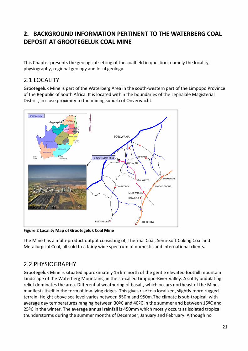
2.1 LOCALITY Grootegeluk Mine is part of the Waterberg Area in the south-western part of the Limpopo Province of the Republic of South Africa. It is located within the boundaries of the Lephalale Magisterial District, in close proximity to the mining suburb of Onverwacht.

Figure 2 Locality Map of Grootegeluk Coal Mine

The Mine has a multi-product output consisting of, Thermal Coal, Semi-Soft Coking Coal and Metallurgical Coal, all sold to a fairly wide spectrum of domestic and international clients.

2.2 PHYSIOGRAPHY Grootegeluk Mine is situated approximately 15 km north of the gentle elevated foothill mountain landscape of the Waterberg Mountains, in the so-called Limpopo-River Valley. A softly undulating relief dominates the area. Differential weathering of basalt, which occurs northeast of the Mine, manifests itself in the form of low-lying ridges. This gives rise to a localized, slightly more rugged terrain. Height above sea level varies between 850m and 950m.The climate is sub-tropical, with average day temperatures ranging between 30ºC and 40ºC in the summer and between 15ºC and 25ºC in the winter. The average annual rainfall is 450mm which mostly occurs as isolated tropical thunderstorms during the summer months of December, January and February. Although no

PRETORIA

BELA BELA MODI MOLLE

RUSTENBURG

LEPHALALE

MOOKGOPONG MOKOPANE

MARKEN

VAALWATER THABAZIMBI

GROOTEGLUK MINE

BOTSWANA

PRETORIA

BELA BELA MODI MOLLE

RUSTENBURG

LEPHALALE

MOOKGOPONG MOKOPANE

MARKEN

VAALWATER THABAZIMBI

GROOTEGLUK MINE

BOTSWANA

WESTERN CAPE WESTERN CAPE EASTERN CAPE EASTERN CAPE NORTHERN CAPE NORTHERN CAPE

FREESTATE FREESTATE KWAZULU NATAL KWAZULU NATAL NORTHWEST NORTHWEST GAUTENG GAUTENG MPUMALANGA MPUMALANGA

LIMPOPO LIMPOPO

LESOTHO

SAWZILAND

CAPE TOWN PORT

ELIZABETH

DURBAN

SOUTH AFRICA LEPHALALE

Grpptegeluk

22

natural drainage networks can be observed in the area, the gentle natural slope of the flat laying landscape is eastwards towards the Mokolo River, which meanders through the region, channelling northward where it flows into the Limpopo River. The vegetation consists of indigenous Bushveld trees and shrubs as well as a variety of grasses, which are adapted to the relatively low rainfall of the region (Bredenkamp et al, 1996)

2.3 REGIONAL GEOLOGY The Zoetfontein Fault in the north and the Eenzaamheid Fault in the south, underlain by the Waterberg Group stratigraphy north of the Eenzaamheid Fault, mark the boundaries of the Waterberg coalfield. The Waterberg Group stretches some 90 km southward culminating in the Waterberg and Sandrivier mountain ranges. North of the Zoetfontein Fault a portion of the Group extends westwards into Botswana, and another portion extends north-easterly to the Blouberg range (Brandl, 1996) Rocks predominantly of the Kransberg Subgroup and the Sandriviersberg Formation are present in the mining area. These are composed of coarse, yellowish, gravely, cross bedded sandstones with ferruginous laminae along the bedding planes. All the classical units of the Karoo Sequence are present in this coalfield and the subdivision of the Karoo Sequence is based mainly on lithological boundaries consisting, in descending order, of the Stormsberg Group, followed by the Beaufort Group, the Ecca Group and the Dwyka Group. The Waterberg Group represents the basin floor (Siepker, 1986). The Karoo groups are further subdivided into lithological units (formations) that have acquired several names over the years. Figure 1 is a 1:250 000 scale map of the regional geology (Brandl, 1996). Starting at the basement the Dwyka Group is mostly encountered as filled depressions in the floor and consists primarily of greyish diamictite and in places rounded pebble conglomerate as well as fluvio-glacial gravels that are products of glacial weathering. The Dwyka Group is only approximately 3m thick in this region.

The Ecca Group overlies the Dwyka Group and can be subdivided into three distinct lithological units, namely the Lower Ecca (Pietermaritzburg Shale), the Middle Ecca (Vryheid Formation) and the Upper Ecca (Volksrust Formation).

The Lower Ecca is composed of shale, siltstone, sandstones and gravels in the lower portions and is approximately 150m thick in the mining area.

The Middle Ecca in the Waterberg coalfield comprises thick yellowish to white, cross-bedded sandstones and siltstones with intercalated dark gray carbonaceous sandy shales and inter-bedded, dull coal seams varying in thickness between 1.5m to 9m. The Middle Ecca is approximately 55m thick in the Waterberg coalfield.

The Upper Ecca, normally characterized by shales of various hues of bluish gray to darker carbonaceous grey, in this area is uniquely interspersed with intercalated and interlaminated bright coal seams. This zone exhibits distinct cyclic sedimentation, notably upward coarsening cycles, starting with a bright coal at the base with the coal to shale ratio gradually decreasing upwards and finally grading into relatively pure shale on top.

The Upper Ecca (Volksrust Formation) shale s show an increase in carbon content with depth, starting with a light bluish grey mudstone on top graduating to very dark grey,

23

carbonaceous shale at its base. The Volksrust Formation in this area is approximately 60m thick.

Figure 3 Regional Geological Map with Grootegeluk locale overlain.

The Beaufort Group in this area comprises of shales of various hues of purple alternating with greenish grey in the upper portion, while light grey mudstones predominate at the base. The unit is approximately 90m thick in the mining area north of the Daarby Fault. The full 90m thickness only occurs north of the Daarby fault in a small rectangular faulted block where the entire sequence has been preserved. The Stormsberg Group overlying the Beaufort Group is subdivided into four distinct lithological units.

The Molteno Formation comprises white, medium to coarse-grained sandstones and is approximately 15m thick in this region.

C a lc a re o u s s a n d sto n e a n d co n g l o m e ra te ; co n s o li d a te d so i l c o ve r e d b y re d s a n d

B a s a lt

Fi n e - g ra in e d c re a m - co lo u re d sa n d s to n e!!

!R e d m u d s to n e a n d si lts to n e

R e d sa n d s to n e a n d c o n g l o m e ra te

V a r ie g a te d sh a l e

M u d st o n e , ca r b o n a c e o u s s h a le , c o a l

G r it ty m u d s to n e , m u d s to n e , sa n d s to n e , c o a l

24

This is succeeded by the Red beds or Elliott formation, consisting primarily of reddish brown to chocolate brown clayey mudstones, marls with interspersed calcareous nodules. Thin white sandstone lenses are also encountered in the upper portions.

The Elliott formation is approximately 90m thick. The Cave Sandstone overlies the Elliott formation or Clarens Formation comprised of

creamy white to yellowish to reddish brown, fine grained, well sorted aeolian sandstone, relatively calcareous with interspersed calcareous nodules. The average thickness is of the order of approximately 80m.

The Drakensberg Basalt or Letaba Formation caps the Clarens Formation. In this area a small lenticular wedge north of the Daarby fault has been preserved. The Letaba Formation is composed of successive lava flows, appearing almost as distinct beds. The lava is dark gray to black but weathers chocolate brown to purple. It has extremely fine crystalline to coarse amygdaloidal tendencies in parts, with amygdales present towards the bases of successive flows. The basalts are fractured and weathering is found between successive lava flows. Thin lenses of sandstone similar to the Clarens also occur between lava flows especially near the base. The Letaba Formation varies from a maximum of 120m to 90m thickness in this region.

2.4 LOCAL GEOLOGY This section describes the nature and distribution of the coal seams and their associated sediments. This is important background information pertinent to the locale of the mine and the material from this deposit being beneficiated.

2.4.1 Volksrust Formation South African coals and coals from other Gondwana provinces tend to be mineral rich, highly variable in rank and organic composition and relatively difficult to beneficiate. These characteristics set them apart from the Carboniferous coals of the northern hemisphere, where the depositional environment was typically hot and humid with the coals originating from coastal swamps comprised of water loving sub tropical equatorial type vegetation and abundant ferns, while the Gondwana region coals were more typically characterized by vegetation ranging from sub arctic through cold to cool temperate deciduous forests to warmer savannah woodlands with reed infested swamps giving rise to generally mineral rich, peat forming swamps.(Falcon,1986) Ultimately the variations in type of vegetation between the northern hemisphere coals and those from the southern hemisphere would be reflected in the maceral compositions of the coals, those from the northern hemisphere being vitrinite rich as opposed to the southern hemisphere coals being inertinite rich. Regional differences within the coal measures in South Africa also exist as a result of differences in the depositional basin, namely the Karoo Basin. Changes as a result of stability, configuration and the nature of the hinterland gave rise to different geometrical developments of seams, different environments of accumulation and different suites of associated minerals and trace elements. The main basin was originally open to the sea, while other smaller derivatives of this main basin, such as those in the Limpopo region, the Springbok Flats and the Waterberg were small shallow fault bound fresh water lakes with relatively similar geological histories allowing relatively consistent qualities for each depositional period. (Falcon et al, 1988) These regional differences

25

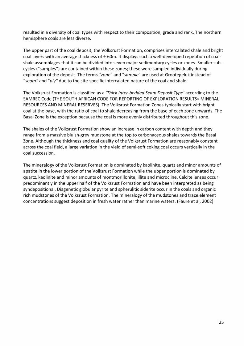
resulted in a diversity of coal types with respect to their composition, grade and rank. The northern hemisphere coals are less diverse. The upper part of the coal deposit, the Volksrust Formation, comprises intercalated shale and bright coal layers with an average thickness of 60m. It displays such a well-developed repetition of coal-shale assemblages that it can be divided into seven major sedimentary cycles or zones. Smaller sub-cycles (“samples”) are contained within these zones; these were sampled individually during exploration of the deposit. The terms “zone” and “sample” are used at Grootegeluk instead of “seam” and “ply” due to the site-specific intercalated nature of the coal and shale. The Volksrust Formation is classified as a ‘Thick Inter-bedded Seam Deposit Type’ according to the SAMREC Code (THE SOUTH AFRICAN CODE FOR REPORTING OF EXPLORATION RESULTS< MINERAL RESOURCES AND MINERAL RESERVES). The Volksrust Formation Zones typically start with bright coal at the base, with the ratio of coal to shale decreasing from the base of each zone upwards. The Basal Zone is the exception because the coal is more evenly distributed throughout this zone. The shales of the Volksrust Formation show an increase in carbon content with depth and they range from a massive bluish-grey mudstone at the top to carbonaceous shales towards the Basal Zone. Although the thickness and coal quality of the Volksrust Formation are reasonably constant across the coal field, a large variation in the yield of semi-soft coking coal occurs vertically in the coal succession. The mineralogy of the Volksrust Formation is dominated by kaolinite, quartz and minor amounts of apatite in the lower portion of the Volksrust Formation while the upper portion is dominated by quartz, kaolinite and minor amounts of montmorillonite, illite and microcline. Calcite lenses occur predominantly in the upper half of the Volksrust Formation and have been interpreted as being syndepositional. Diagenetic globular pyrite and spherulitic siderite occur in the coals and organic rich mudstones of the Volksrust Formation. The mineralogy of the mudstones and trace element concentrations suggest deposition in fresh water rather than marine waters. (Faure et al, 2002)

26

Figure 4 Cyclic Sedimentary Subdivision of Coal sequence for the Volksrust Formation.

2.4.2 Vryheid Formation The Vryheid Formation ( 55m thick) forms the lower part of the coal deposit and comprises carbonaceous shale and sandstone with inter-bedded dull coal seams varying in thickness from 1.5m to 9m. The Vryheid Formation is classed as a ‘Multiple Seam Deposit Type’ according to the SAMREC Code. There are five coal seams or zones in the Vryheid Formation, all of which are composed predominantly of dull coal with some bright coal developed at the base of Zones 2, 3 and 4. Due to lateral facies changes and changes in the depositional environment, these zones are characterized by a large variation in thickness and quality. It is inferred that these zones deteriorate in a westward direction on the Mining Rights Area and Prospecting Rights Area.

27

Figure 5 Cyclic Sedimentary Subdivision of Coal sequence for the Vryheid Formation

Zone 3 is the best-developed dull coal zone within the Mine Lease Area, reaching a maximum thickness of 8.9m. The basal portion of this zone yields a small fraction that has semi-soft coking coal properties.

Zone 2 is, on average, 4m thick and reaches a maximum thickness of 6m in the Mine Lease Area. The basal portion of this zone also yields a fraction that has semi-soft coking coal properties. This zone is the most constant of all the Vryheid coal zones across the entire Waterberg Coal Field regarding thickness.

Zone 1, the basal Vryheid coal zone, has an average thickness of 1.5m, but varies quite rapidly being the lower-most coal layer in the sequence.

2.4.3 Classification of the Volksrust and Vryheid Formation Coals

Coal is a sedimentary rock primarily accumulated as peat, comprising macerals, minerals, water and gases in submicroscopic pores. Macerals are organic remnants derived from plant tissues and exudates that have been subjected to decay, incorporated into sedimentary strata, compacted, hardened, and chemically altered by natural processes. Coal is an aggregate of microscopically

28

distinguishable, physically distinctive, and chemically different macerals and minerals. Coal is therefore a heterogeneous mixture of diverse substances derived from the diversity of source material prevalent in the peat swamp accumulations. Coal can be contrasted and classified on the basis of variations in the proportions of its identifiable components and referred to as a classification according to type, as well as the degree of metamorphism (geological alteration processes having affected the coal properties) and are then referred to as classification according to rank. The characterization can be approached from two levels, empirical and fundamental analysis (Falcon, 1987). The empirical determinations are analytical classifications based on two sets of analysis. 1. Proximate analysis used for the determination of:

moisture i.e. water entrapped within the structure retained within the pores and fissures after all surface moisture has been removed,

the ash content referring to residual minerals and after the complete combustion of the coal,

the volatile matter derived from both the organic matter and the inorganic matter, the organic matter being responsible for the production of oils, tars, hydrocarbon gasses, hydrogen and carbon oxides which are released as the temperature is increased and the inorganic matter producing incombustible volatiles such as carbon dioxide from carbonate minerals, sulphur oxides from pyrites and water from some clay minerals.

Fixed carbon, referring to the organic content of coal remaining after devolatization,

2. Ultimate analysis, where the coal is analyzed to determine its ultimate chemical components with reference to the elements carbon, hydrogen, nitrogen, oxygen and sulphur. In addition to the former analyses, the calorific value of the coal, one of the most important commercial parameters which is a measurement of its potential heat content or energy expressed in mega joules per kilogram (in South Africa), British Thermal units per pound of coal (Btu) in the United Kingdom or kilo-calories per kilogram of coal (USA, Europe and the Far East) is also done. The second level of evaluation pertains to a classification relating to the fundamental composition of the coal, its organic and inorganic components and unlike empirical analyses this requires the microscopic evaluation of coal. The fundamental composition of coal is subdivided into three main categories, the organic matter, mineral matter and rank or degree of metamorphism. Microscopically identifiable units relating to the fragmented and partially decomposed organic remains of vegetative matter are called macerals, of which wide varieties occur. These macerals are subdivided into three main groups, namely, the vitrinite group, the liptinite (or exinite) group and the inertinite group based on their common chemical, physical, optical and technological properties. However considering the information available at the exploration stage, no analysis with respect to ultimate analyses or petrographic analyses would have been done. The empirical data i.e., proximate analysis, was according to the standard specification for the classification of coals as promulgated by the American Society of Testing Materials. Classification according to grade relates to the compositional proportions of both the different organic substances and the mineral constituents, while rank classification is independent of maceral and mineral content since only the alteration of organic matter by the metamorphic process is considered. Bearing the composition of coal in mind, higher density values with the same ash value

29

as a low density fraction could be as a result of maceral distribution as well as differences in maturity indicating the possibility of some alteration by metamorphic processes reducing the volume of the original material. Thus it may be possible to increase the density of the material while the ash yield remains constant.

Figure 6 Comparison of Northern hemisphere coals, their rank and South African coals

The International Classification of In–Seam coal developed by the ECE-United Nations Working Party on Coal undertaken by the “Coal Committee “was designed to permit the classification of coals to contribute to the characterization of coal deposits. The systemization was based on the joint evaluation of three fundamental characteristics, rank (maturation, degree of coalification), and the petrographic composition of the coals as well as the grade of the coal referring to inclusive impurities within the coal. Initial results of the type classification for the major stratigraphic units, the Volksrust and Vryheid Formations’, were based on empirical data derived from calculations as specified in the standard specification for the classification of coals by rank, as promulgated by the American Society of Testing Materials. The formulations suggested for an approximation of the required properties were used in this evaluation to deduce recognizable variations in the coal rank. These are rank classes in the individual zones and their representative percentages highlight the differences between the two stratigraphic units. Although Zone 5 is deemed to be part of the Volksrust Formation (formerly known as the Upper Ecca) the graphic appears to indicate a transition from the Volksrust Formation to the Vryheid Formation, an evaluation of the sub cycles (individual samples) of this Zone may serve to indicate the transition or change more clearly.

30

Figure 7 Coal type zone compositions of Waterberg coal field zones based on empirical data evaluation and ASTM standards.

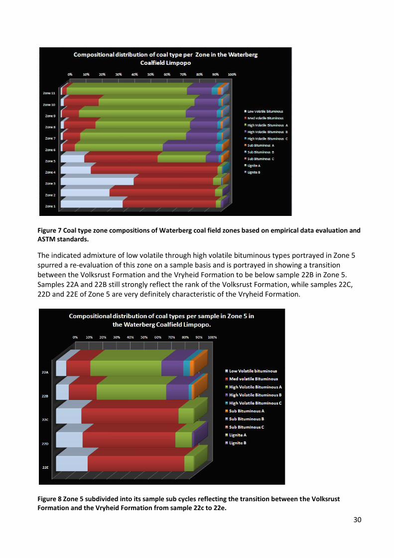
The indicated admixture of low volatile through high volatile bituminous types portrayed in Zone 5 spurred a re-evaluation of this zone on a sample basis and is portrayed in showing a transition between the Volksrust Formation and the Vryheid Formation to be below sample 22B in Zone 5. Samples 22A and 22B still strongly reflect the rank of the Volksrust Formation, while samples 22C, 22D and 22E of Zone 5 are very definitely characteristic of the Vryheid Formation.

Figure 8 Zone 5 subdivided into its sample sub cycles reflecting the transition between the Volksrust Formation and the Vryheid Formation from sample 22c to 22e.

31

This evaluation however, may have presented a clearer overview of the admixtures of different possible coal types defined only on the basis of empirical data in the overall composition of the coal zones from both the Volksrust and Vryheid Formations but cannot be used for characterization and final classification purposes. The final classification based on the ECE-UN classification, 1998, categorizes these coals to a Low to Medium Grade on the basis of ash yield, Medium Rank, and Ortho Bituminous Coal in terms of maturity. The boundary limits for the main divisions and sub divisions were based on Vitrinite mean random Reflectance percent and Gross Calorific Value in MJ/kg with analytical parameters for these methods conforming to ISO 7402-5 [43] AND 1928 [39] standards Respectively. Table 1 Classification of Waterberg Coal Zones 1 through 11 based on the ECE- UN Standards.

2.4.4 Factors Controlling Geological Continuity As the Waterberg Coal Field is fault bounded along its southern and northern margins it can be referred to as a graben deposit, with the Eenzaamheid Fault forming its southern limit and the Zoetfontein Fault forming its northern boundary. The Daarby Fault, with a down-throw of approximately 350m towards the north-east, divides the Coal Field into a deep north-eastern portion and a shallow south-western portion. Sedimentological facies changes also influence the continuity of the sediments and their qualities. This is especially prevalent in the Vryheid Formation Coal Zones with deterioration in coal development towards the west of the Mining Rights Area and the Prospecting Rights Area.

Figure 9 Regional Structure of the Waterberg Coalfield

32

3. MINING This chapter presents the mining background and assumptions as seen against the sampling strategy in the coalfield, and it summarises the geological factors that may impact on the beneficiation properties of the coal in this coalfield. Grootegeluk Mine is a surface mining operation where a series of parallel benches are advanced progressively across the deposit via a process of drilling, blasting, loading and hauling with truck and shovel fleets. The pit was established on the open cast able portion of the Waterberg Coal Field, immediately west of the Daarby Fault. It was originally brought into production to deliver a blend coking coal product to the ISCOR Steel Works. The erection of Eskom’s Matimba Power Station and Iscor’s Saldanha Steel Manufacturing Plant resulted in a multi-product operation that produces Thermal and Metallurgical Coal in addition to the Semi-Soft Coking Coal. The area west of the Daarby Fault was selected for mining due to low overburden thicknesses giving an acceptable stripping ratio. There are relatively few structural complications and quality parameters are fairly constant in the area. Mining activities extend down to Zone 2 of the Vryheid Formation.

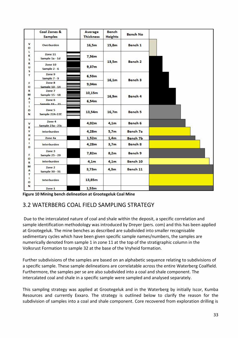
3.1 MINING FACTORS AND ASSUMPTIONS From the geological profile of the Volksrust Formation and the intercalated nature of the coal and shale, selective mining could not be considered as an option. Bulk opencast mining of the Volksrust Formation was the only feasible mining method. In 1987 Grootegeluk Mine changed from mining benches with fixed elevations to mining benches that coincide with geological contacts for the roof and floor of each mining bench in order to provide the beneficiation plants with a run-of-mine feed of less variable quality. These geological contacts coincide with zone boundaries and simultaneously provide mine benches in the Volksrust Formation with an average height varying from 14m to 17m. The change facilitated selective mining of Zone 5, which is characterized by a high phosphorous content and simultaneously also ensured that the floor of each mine bench coincides with a prominent shale layer, providing a smooth surface for equipment movement, while protecting the underlying coal from surface oxidation. Due to the low regional dip of the strata in a south easterly direction, following these geological contacts while developing the pit westwards also assists storm water drainage to the sump at the pit bottom. Although faulting in the Volksrust Formation does not seriously affect mining operations in the open pit operation at this stage, the increase in depth of weathering associated with such faulting does produce problems because of the clay (weathered shale and decomposed coal) remnants in such areas.

33

Figure 10 Mining bench delineation at Grootegeluk Coal Mine

3.2 WATERBERG COAL FIELD SAMPLING STRATEGY Due to the intercalated nature of coal and shale within the deposit, a specific correlation and sample identification methodology was introduced by Dreyer (pers. com) and this has been applied at Grootegeluk. The mine benches as described are subdivided into smaller recognisable sedimentary cycles which have been given specific sample names/numbers, the samples are numerically denoted from sample 1 in zone 11 at the top of the stratigraphic column in the Volksrust Formation to sample 32 at the base of the Vryheid formation. Further subdivisions of the samples are based on an alphabetic sequence relating to subdivisions of a specific sample. These sample delineations are correlatable across the entire Waterberg Coalfield. Furthermore, the samples per se are also subdivided into a coal and shale component. The intercalated coal and shale in a specific sample were sampled and analysed separately. This sampling strategy was applied at Grootegeluk and in the Waterberg by initially Iscor, Kumba Resources and currently Exxaro. The strategy is outlined below to clarify the reason for the subdivision of samples into a coal and shale component. Core recovered from exploration drilling is

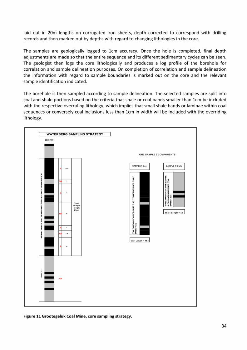
34

laid out in 20m lengths on corrugated iron sheets, depth corrected to correspond with drilling records and then marked out by depths with regard to changing lithologies in the core. The samples are geologically logged to 1cm accuracy. Once the hole is completed, final depth adjustments are made so that the entire sequence and its different sedimentary cycles can be seen. The geologist then logs the core lithologically and produces a log profile of the borehole for correlation and sample delineation purposes. On completion of correlation and sample delineation the information with regard to sample boundaries is marked out on the core and the relevant sample identification indicated. The borehole is then sampled according to sample delineation. The selected samples are split into coal and shale portions based on the criteria that shale or coal bands smaller than 1cm be included with the respective overruling lithology, which implies that small shale bands or laminae within coal sequences or conversely coal inclusions less than 1cm in width will be included with the overriding lithology.

Figure 11 Grootegeluk Coal Mine, core sampling strategy.

CORE

SA

MP

LE 2

NS

ONE SAMPLE 2 COMPONENTS

SAMPLE 1 Coal SAMPLE 1 Shale

COAL

PO

RTIO

N RE

MO

VED,

NO

TE T

HAT

IT C

ONT

AIN

S M

INO

R SH

ALE

BAND

S <1

cm

SHAL

E PO

RTIO

N O

F SA

ME

SAM

PLE

ALSO

CO

NTAI

NING

MIN

OR

COAL

BA

NDS

< 1c

m

Shale Length = 7.5

Coal Length = 13.5

NS 1.5

S 4

NS 5

S 1

WATERBERG SAMPLING STRATEGY

ORI

GIN

AL

SAM

PLE

1 D

ELIN

EATE

D AC

CORD

ING

TO

CYC

LIC

SEDI

MEN

TATI

ON

S 4.5

Total Sample length 21cm

NS 1

S 4

35

The single correlated sample above is broken into two components, a coal portion and a shale portion, analyzed separately and then re-composited to obtain a single representative value for the sample from the separate wash tables. The coal samples are washed (sink floated) from RD 1.35 g/cc to 2.20 g/cc while the shale samples are washed from RD 1.50 g/cc to 2.20 g/cc. After the float/sink tests and proximate analysis have been completed the results of the individual coal and shale components of samples are composited to obtain a weighted representative wash table for the entire sample.

Figure 12 Grootegeluk wash table configuration.

The re-constituted sample data is then used for further evaluation and compilation of the geological model.

36

In summary a flow chart of the processes and data available from the exploration borehole to the laboratory is included to illustrate the recorded data that could be evaluated.

Figure 13 Flowchart of processes and data available from an exploration borehole through the laboratory and back to the original site.

3.3 GEOLOGICAL FACTORS ASSOCIATED WITH BENEFICIATION

3.3.1 Background South African coals contain only small amounts of spore coats, leaf cuticles and other remains of leaves and seeds, which form parts of black durain and clarain, which are rarely found (The South African Coal Processing Society, 2002.). South African coals are mixtures of vitrain and grey durain and vary from coals with preponderant vitrain (bright coal) through various banded mixtures with grey durain to pure durain (dull coal). In the Waterberg however, specifically the Volksrust Formation (Grootegeluk Formation or previously known as the Upper Ecca) an abundance of vitrain occurs. Maceral analyses of the coal seams and the inter-bedded carbonaceous mudstones show that vitrinite is the dominant maceral (up to 90 %), whereas inertinite, liptinite and reactive semi-fusinite generally occur in minor proportions.( Faure et al, 1996). Vitrinite content increases upward in the formation, with a concomitant decrease in inertinite (including reactive semi-fusinite) from around 60% inertinite at the base of the formation. The upward increase in the vitrinite concentration is associated with a decrease in the energy of the depositional environment, which would have been instrumental in the preservation of the vitrinite. Problems relating to low ash semi soft coking coal cut densities and associated parameters exist as a result of the distribution and quantity of near density material in the lower density regions of the bright coals. Near density material is material within ±0.1 g/cc of the cut point relative density at which the coal is being washed as defined in “Coal Preparation in South Africa 2002”

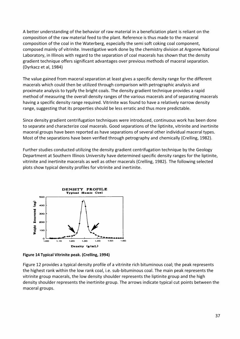
37

A better understanding of the behavior of raw material in a beneficiation plant is reliant on the composition of the raw material feed to the plant. Reference is thus made to the maceral composition of the coal in the Waterberg, especially the semi soft coking coal component, composed mainly of vitrinite. Investigative work done by the chemistry division at Argonne National Laboratory, in Illinois with regard to the separation of coal macerals has shown that the density gradient technique offers significant advantages over previous methods of maceral separation. (Dyrkacz et al, 1984) The value gained from maceral separation at least gives a specific density range for the different macerals which could then be utilized through comparison with petrographic analysis and proximate analysis to typify the bright coals. The density gradient technique provides a rapid method of measuring the overall density ranges of the various macerals and of separating macerals having a specific density range required. Vitrinite was found to have a relatively narrow density range, suggesting that its properties should be less erratic and thus more predictable. Since density gradient centrifugation techniques were introduced, continuous work has been done to separate and characterize coal macerals. Good separations of the liptinite, vitrinite and inertinite maceral groups have been reported as have separations of several other individual maceral types. Most of the separations have been verified through petrography and chemically (Crelling, 1982). Further studies conducted utilizing the density gradient centrifugation technique by the Geology Department at Southern Illinois University have determined specific density ranges for the liptinite, vitrinite and inertinite macerals as well as other macerals (Crelling, 1982). The following selected plots show typical density profiles for vitrinite and inertinite.

Figure 14 Typical Vitrinite peak. (Crelling, 1994)

Figure 12 provides a typical density profile of a vitrinite rich bituminous coal; the peak represents the highest rank within the low rank coal, i.e. sub-bituminous coal. The main peak represents the vitrinite group macerals, the low density shoulder represents the liptinite group and the high density shoulder represents the inertinite group. The arrows indicate typical cut points between the maceral groups.

38

Figure 15 A typical Vitrinite / Inertinite Gondwana Coal. (Crelling, 1994)

The second selected density profile Figure 14 Typical Vitrinite peak. (Crelling, 1994) is that of an inertinite rich coal, the original sample obtained from South Africa and representative of a typical Gondwana coal. The highest peak represents the density of the vitrinite, while the bulk of the sample is representative of the inertinite group macerals on the high density side of the vitrinite. A further consideration with regard to these coals, relates to the physical properties of the coal samples in their raw state, the main property of concern being the porosity of these coals and their susceptibility to absorbing moisture in the beneficiation process which contributes to the displacement of products as a result of altered relative densities in the process. Reiterating, porosity in coal can be defined as the proportion of the total volume of the coal occupied by water or gas (Levine, 1993). Porosity occurs in the matrix of the coal and as fissures and fractures in the coal. Invariably the matrix porosity is not associated with coal cleats, fractures or joints and as such the matrix porosity is largely in the micro-pore region with pore diameters of less than 2nm although some pores are microscopically visible between individual particles in inertinite masses. (Parkash et al., 1986) Fracture porosity in coal on the other hand refers to the network of cleats formed during coalification and is usually in the macro-pore range with pores greater than 50nm (Ting, 1977; Close, 1993; Laubach et al., 1998). Considering the foregoing, and a hypothetical situation using an air dried sample as a starting point and the total moisture content of this sample having been determined, the moisture content value would be reasonably representative of a portion of the total porosity. The actual total volumes of solids and voids are unknown since the best results can only be determined through the use of gas pycnometry on a pulverized absolutely dry sample, using helium as the gaseous medium because it readily diffuses into the small pores. Starting with the original run of mine or core material, the feed would have its highest void/moisture content, as the material is broken down through the crushing process to a top-size suitable for the beneficiation plant. The fracture porosity per unit mass is partially destroyed by crushing and thus reduced, but the micro porosity of the individual maceral components are unaffected.. The adsorption potential however would be increased due to the greater surface area exposed but this would not be a problem since mechanical drainage and air drying would be simplified. The micro-pores however would not surrender their moisture content as easily, and it is this property, considering that these pores were initially penetrated by diffusion which contributes to the complication and incorrect density determinations of the material. Absorption within the micro

39

pores of crushed and dried material prior to float and sink testing would contribute to the retention of flotation medium which would result in material reporting to higher densities than their apparent true densities thus aiding in the misplacement of products at specific densities.

40

4. LITERATURE REVIEW This Chapter presents an overview of previous work concerned with density, moisture and porosity in coal. An assessment of the problems related to tonnages produced as opposed to the original planned and budgeted figures, as well as attempts at reconciling the final data with the original basic data used for the determination of resources and reserves, has highlighted critical deficiencies in the entire process. These deficiencies are related to both the initial evaluation methods and the mining process. (Roux, 2010) The mentioned assessments are dealt with in Chapter 7.3.3. The simplified schematic included below is a hypothetical example illustrating the basic source of the problem. I.e. the originally determined basic data has given values to a proposed mining block on which certain assumptions with regard to material to be recovered from this block are estimated. The density values used are from Archimedes derived SG in the first case representing the targeted budget while the second density value representing the mined material was derived from the reconciliation of mined volumes and weightometer measured tons. In Figure 16, the TARGET Budgeted yield tonnages of commercially saleable products are higher relative to the ACTUAL Recovered tonnages where product yields are considerably lower.

Figure 16 Schematic depicting two scenarios with reference to volumetric size being equal but different tonnages. These scenarios represent the outcome with regard to tonnages of the same block: in the first case, Archimedes density assigned to the raw material and in the second scenario, actual recorded tonnages recovered. The resultant losses in the second scenario are attributable to the reconciled density derived from recovered tonnage from the volume mined.

This simplified schematic illustrates the magnitude of inaccuracies that can be realized through an incorrect or questionable basic density value applied to the basic geometrics of a proposed mining block and the subsequent consequences with regard to projected product recoveries. The exercise also highlights the fact that reconciliation should start at the source and that errors that may be considered minor at source can have a major impact on forecasts. An example of an assumed minor mistake in density determination is the fact that a 0.1 g/cc, considered as a minor amount, translates into a 10% over or under estimation of expected

41

tonnages. Now consider another example taken from the foregoing illustrated schematic showing a 15% loss on the target, when this is extended to a life of mine calculation, the result can lead to a shortened life of mine. A projected life of mine of 40 years would result in depletion of mineable material after 34 years as a result of the initial 15% over estimation of available reserves based on the values illustrated in Figure 16 where the in situ raw relative density used for the determination of the mineable material has been overestimated. Problems experienced during the course of time at Grootegeluk coal mine in the Waterberg coalfield led to a research project relating to the prediction of products from this coalfield and the differences noted between the predicted values and actual plant production.(Roux, 2012) The project concentrated mainly on the beneficiation aspects and in- house determined correlation factors that were applied to specific regions in the mine and was based on the optimal yield and cut density prediction for semi soft coking coal and power station middling’s coal in the Waterberg Coalfield, Limpopo, (Roux. 2012) The results of this research allowed the negation of a collection of different correlation factors relating to the sources of origin of the raw feedstock material historically derived from the reconciliation of final products against the predicted products for individual mining benches. Tonnages of the various products were determined in-situ. Reconciliation of the final products after beneficiation presented a multitude of problems due to extraneous uncontrollable factors, which resulted in the introduction of correlation factors to account for inexplicable differences (Dreyer, 1994). Relatively accurate correlation factors were determined per mining bench, provided that the material being beneficiated was consistently supplied from the same source and the same vertical sequence. The behavior of material from a particular bench, mined over a relatively long period consistently, was assessed and values adjusted via the determined correlation factors to ascertain the products from a particular source.(Roux, 2006) The probable yield of this raw material was then determined. An important aspect was that the correlation factors derived were suitable while the beneficiation process remained the same, thus these factors would have to be adjusted after any changes or improvements within the beneficiation environment were implemented. An example of such a change would be the introduction of spiral modules to improve overall efficiency and recovery. Conversely changes also had to be made if and when the nature of the raw run of mine material changed, examples being related to oxidation and weathering or lateral facies changes within the depositional environment. Four sets of factors had to be determined to accommodate the different materials for each product required as well as for grade control and budgeting purposes. Modeled values had to be adjusted for the 4 different sources of raw material. Examples of this as follows: Bench 2 weathered with a coking coal correlation factor of 62% and middling (power station coal) correlation factor of 94.57%, normal bench 2 materials, 71.95% and 95.65% respectively, bench 3, 74.77% and 143.07% and bench 4 with 70.24% and 113.20% for middling (Power station coal). It is relevant to note that the discussed values are only relevant to one of the beneficiation plants, Grootegeluk 1, semi soft coking coal and power station coal beneficiation plant. Each respective plant with its unique string of products and top sizes of material broken for beneficiation had their

42

own unique set of correlation factors. However, due to increased demand, greater volumes of material being required and mining pit geometry factors having to be honored, the practice of selectively mining one bench or portions of a bench over a reasonable period of time to sustain the methodology of controlling correlation factors for the various benches could not be sustained. Material from two or more locations from the various mining benches had of necessity to be blended as raw feedstock to the beneficiation plant. Predictions of probable product for budgeting and forecasting purposes became nigh impossible since the old system of correlation factor application failed miserably. The correlation factors were reduced to a single correlation factor specific to a specific beneficiation plant process. The correlation factor was based on the beneficiation plant’s capabilities and efficiency, the physical nature of the run of mine material, its reduction to a specific top size before being processed and the actual results obtained, irrespective of the origin of the material. The research and implementation of this methodology at this mine improved the predicted values to such an extent that the individual beneficiation plant’s products were conforming with the predicted values, after the plant specific correlation factor had been applied to the theoretically determined product yields (Roux, 2011, 2012, 2013, In house confidential reports) The probability that the correlation factor can be removed entirely, however still exists, since the correlation factor, although plant specific is based on plant production results, a deficiency equivalent to the difference between the correlation factor and the 100% theoretical value determined from cumulative wash table remained. This difference at the time was approximately 17.82%. Should this difference be accommodated and negated then the reconciliation loop will be completed and will support the values obtained from the geological model resulting in increased confidence in the credibility of the data obtained and used. Addressing this loss leads to the evaluation of the accuracy of tonnages determined for the feed material from a specific area within the mine before extraction and dispatch to the various beneficiation plants. The uncertainty though relates to the reconciliation of tonnages measured on extraction with volumes extracted. This approach reverts to the exploration phase and the determination of gross in situ tonnages and the various applicable geological loss factors applied to accommodate physical losses not related to the mechanics of the mining operation resulting in recoverable run of mine reserves. Referring to the hypothetical example shown in Figure 16 presented earlier, the volume of rock removed has remained constant in both cases, the predicted tonnages based on the predetermined relative density of the host, however, differ in terms of the actual tons recovered as does the relative density determined from this mined volume. This assumes that no material has been lost in transit from the mining face to the beneficiation plant. The only component that could contribute to the reduced measured tons to equate them with the predicted tonnage is moisture. The moisture content referred to represents the difference in moisture content of the host coal at the exploratory stage when the Archimedes density was determined and the moisture content at the time of mining. No further density determinations apart from laboratory Archimedes SG determinations to verify the field values were done. The densities thus obtained were used for the gross in-situ tonnage derivation. It should be noted that the moisture content of the host fluctuates under different conditions, for example a receding ground water table will allow a certain amount of drainage of the host. Core exposed to atmospheric conditions without impeccable preservation

43

would also loose adventitious moisture. The moisture lost represents voids that have drained; therefore the host has an effective inherent porosity which makes it a critical factor influencing the determination of in situ relative density.

4.1 DENSITY AND MOISTURE Although the effect of mineral matter (ash yield) has long been recognized and recent studies (Roux, 2012) have revealed a relationship between ash and density based on analytical data evaluated from proximate analysis on air dried samples. Analyses done by the University of Illinois as early as 1916 on relative density (at that stage referred to as Specific Gravity) under varying conditions of moisture content added a whole new perspective with regard to the variability of density to results obtained. (Nebal, 1916) The American Society for Testing and Materials’ book of standard definitions lists no less than forty definitions for density based on mass per unit volume. The British Standards Institute has reduced this to fourteen types of densities. The determination of the mass of an object is relatively straightforward; the determination of the volume however is not that simple. The volume of an object, whether a single piece or a mass of finely divided powder, is a concept that cannot be ascribed to a single, neat definition. A typical definition of volume in most dictionaries is described vaguely as ‘the space occupied by an object.’ McGraw-Hill’s Dictionary of Scientific and Technical Terms (1984) do not say much more, their definition merely relates the object to three dimensional spaces “A measure of the size of a body or definite region in three dimensional space….” In order to appreciate the various conditions under which volume is defined, particle technology’s lexicon used for these definitions can be found in the British Standards Institute (BSI,1991) and the American Society for Testing and Materials (ASTM,1994) documents. Here the ‘volume’ of a material is described as the summation of several rigorously defined elemental volumes. A cylindrical length of rock core can be used as an example of an object that contains all types of elemental volumes and differences in material volume according to the measurement technique, measurement method, and conditions under which the measurements are performed. The rock core obviously, is solid material having a volume that can be calculated after measuring its length and its diameter from which its area can be determined. However, it also contains surface irregularities, small fractures, fissures, and pores that both communicate with the surface and pores that are isolated within the structure. Voids that connect to the surface are referred to as open pores while interior voids inaccessible from the surface are referred to as closed pores. Surface irregularities compose another type of void volume. For example, assume the bulk volume of the core is determined from linear measurements of its length and area. The value of volume determined in this way is limited in accuracy because the surfaces are not perfect. If a perfect plane were to be laid on one of the surfaces of the core, there would be many voids sandwiched between the two surfaces.

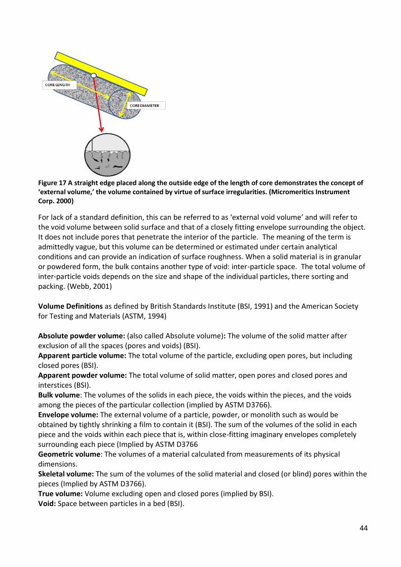
44

Figure 17 A straight edge placed along the outside edge of the length of core demonstrates the concept of ‘external volume,’ the volume contained by virtue of surface irregularities. (Micromeritics Instrument Corp. 2000)

For lack of a standard definition, this can be referred to as ‘external void volume’ and will refer to the void volume between solid surface and that of a closely fitting envelope surrounding the object. It does not include pores that penetrate the interior of the particle. The meaning of the term is admittedly vague, but this volume can be determined or estimated under certain analytical conditions and can provide an indication of surface roughness. When a solid material is in granular or powdered form, the bulk contains another type of void: inter-particle space. The total volume of inter-particle voids depends on the size and shape of the individual particles, there sorting and packing. (Webb, 2001) Volume Definitions as defined by British Standards Institute (BSI, 1991) and the American Society for Testing and Materials (ASTM, 1994) Absolute powder volume: (also called Absolute volume): The volume of the solid matter after exclusion of all the spaces (pores and voids) (BSI). Apparent particle volume: The total volume of the particle, excluding open pores, but including closed pores (BSI). Apparent powder volume: The total volume of solid matter, open pores and closed pores and interstices (BSI). Bulk volume: The volumes of the solids in each piece, the voids within the pieces, and the voids among the pieces of the particular collection (implied by ASTM D3766). Envelope volume: The external volume of a particle, powder, or monolith such as would be obtained by tightly shrinking a film to contain it (BSI). The sum of the volumes of the solid in each piece and the voids within each piece that is, within close-fitting imaginary envelopes completely surrounding each piece (Implied by ASTM D3766 Geometric volume: The volumes of a material calculated from measurements of its physical dimensions. Skeletal volume: The sum of the volumes of the solid material and closed (or blind) pores within the pieces (Implied by ASTM D3766). True volume: Volume excluding open and closed pores (implied by BSI). Void: Space between particles in a bed (BSI).

45

Traditionally the ordinary method of determining the relative density of a solid, such as coal, is to weigh it in air, then immerse it in water and weigh it again, the relative density being equal to the ratio of the weight in air to the loss of weight in water. A more specific definition of Relative Density (RD) (Preston and Sanders, 2005) At a temperature of 50 C, the density of water is 1.0g/cc, thus the relative density of a material is its density relative to the density of water at 50 C. This property is a ratio, thus dimensionless, and is numerically equivalent to the density of the material expressed in grams per cubic centimeter. All relative density determinations require the mass and the volume of the material to be measured. The mass determination is simple; the volume determination however as discussed earlier, both in regard to measurement and understanding in heterogeneous materials such as coal is relatively complex. This relates primarily to the porosity of coal and the variable degree to which different methods cope with this aspect of the determination.

Figure 18 Illustration of various volume types. At the top left is a container of individual particles illustrating the characteristics of bulk volume in which inter-particle and “external” voids is included, at the top right is a single porous particle from the bulk sample. The particle cross-section is shown surrounded by an enveloping band. In the illustrations at the bottom, black areas shown are analogous to volume. The three illustrations at the right represent the particle. Illustration A. is the volume within the envelope, B is the same volume minus the “external” volume and volume of open pores, and C is the volume within the envelope minus both open and closed pores. (Webb, 2001)

Since coal is porous, most of the contained moisture is held mechanically in its pores. The pores may be interconnected or isolated, interconnected pores contribute to permeability thus, when coal is dried, its permeability allows some of the moisture to leave the pores, which become filled with air; if the dry coal is placed in water, the air in the pores is displaced by the water, and the coal becomes saturated. Under such circumstances the length of time coal is immersed in water before it is weighed affects the value obtained for the relative density of the coal. ‘True’ or ‘Absolute’ Relative Density (Preston and Sanders, 2005) True or absolute relative density should only be used to describe the relative density of a volume of pore free coal which by implication means that whichever method is used in determining the volume of the sample, the

46

medium used must occupy all the pores which in practice is very difficult. Helium being the smallest atom has the best probability of penetrating the greatest number of pores, thus the helium density method is the recognized method for determining this parameter. The availability of consistently reliable true or absolute relative density values for coal would make the estimation of in situ relative density a straightforward process. ‘Apparent’ or ‘Coal Particle’ Relative Density Apparent relative density describes the relative density of lump coal which may contain pores, fissures and moisture of which the preservation in the actual sample may be variable, tending to give unreliable results when determined by the displacement of water, by the lump coal in a bath. A more precise determination through the use of the mercury density method can be obtained, but similar to the helium method, the equipment required is not always available. In Situ Relative Density In situ relative density refers to the relative density of the coal in the ground. The coal under confining pressure contains pores and fissures filled with water and dissolved gasses. The relative density measurement of the coal in situ, required, is the value that should be used for the estimation of coal resources and reserves. This value may be calculated from the coal thickness (in situ), the core diameter and the mass of impeccably preserved core lengths. The Australian Standard method of determining coal density is most commonly used and although the method is cheap and easy to apply, the state of the sample, when tested, does not simulate the in situ condition of the coal, because, the sample is ground to -212µm removing fissures and some pores, it is also air dried retaining some of it’s in situ moisture. The moisture thus retained may well be representative of the inherent moisture of the coal sample as determined when proximate analysis is performed on the same sample. The method involves measuring the liquid displacement, either in a density bottle or volumetric flask, thus determining the volume of the ground coal sample; this is then related to the original weighed mass. The major problem with the method is the inability of the liquid to occupy all pores within the coal and thus displace all air and water. The result gives neither absolute relative density nor in situ relative density although it is probably closer to the absolute relative density. Under rigorously controlled conditions, the standard density bottle method may give results closely approximating the true or absolute relative density for coal expressed on the air dry basis. This standard method does not replicate the conditions to be met in a determination of in situ relative density since the values obtained are tested on an air dry basis, whereas the reserves of coal in situ are not (Preston and Sanders, 2005 ). The use of standard relative density in reserve calculations has been estimated to result in an overestimation of reserves of between 2.5% and 4.5%. In order to convert the standard relative density to an in situ relative density, the sample needs to be reconstructed to simulate original conditions especially with relevance to the original volume restoring the pores and fissures destroyed in the grinding process. The reduction in volume of the sample has a greater effect on the relative density than the loss of mass held in that volume. If the voids are restored to their original state and refilled with water, both the volume and mass will increase, the volume however will increase at a rate higher than the mass and thus the sample density will decrease trending towards 1, the relative density of water. The most critical bit of information required here, relates to the in situ moisture content of the sample since this would be critical to the calculation of densities, reserves, coal handling mass calculations and to the

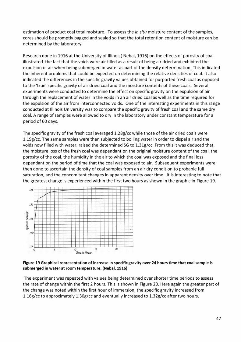
47

estimation of product coal total moisture. To assess the in situ moisture content of the samples, cores should be promptly bagged and sealed so that the total retention content of moisture can be determined by the laboratory. Research done in 1916 at the University of Illinois( Nebal, 1916) on the effects of porosity of coal illustrated the fact that the voids were air filled as a result of being air dried and exhibited the expulsion of air when being submerged in water as part of the density determination. This indicated the inherent problems that could be expected on determining the relative densities of coal. It also indicated the differences in the specific gravity values obtained for purported fresh coal as opposed to the ‘true’ specific gravity of air dried coal and the moisture contents of these coals. Several experiments were conducted to determine the effect on specific gravity on the expulsion of air through the replacement of water in the voids in an air dried coal as well as the time required for the expulsion of the air from interconnected voids. One of the interesting experiments in this range conducted at Illinois University was to compare the specific gravity of fresh coal and the same dry coal. A range of samples were allowed to dry in the laboratory under constant temperature for a period of 60 days. The specific gravity of the fresh coal averaged 1.28g/cc while those of the air dried coals were 1.19g/cc. The same samples were then subjected to boiling water in order to dispel air and the voids now filled with water, raised the determined SG to 1.31g/cc. From this it was deduced that, the moisture loss of the fresh coal was dependant on the original moisture content of the coal the porosity of the coal, the humidity in the air to which the coal was exposed and the final loss dependant on the period of time that the coal was exposed to air. Subsequent experiments were then done to ascertain the density of coal samples from an air dry condition to probable full saturation, and the concomitant changes in apparent density over time. It is interesting to note that the greatest change is experienced within the first two hours as shown in the graphic in Figure 19.

Figure 19 Graphical representation of increase in specific gravity over 24 hours time that coal sample is submerged in water at room temperature. (Nebal, 1916)

The experiment was repeated with values being determined over shorter time periods to assess the rate of change within the first 2 hours. This is shown in Figure 20. Here again the greater part of the change was noted within the first hour of immersion, the specific gravity increased from 1.16g/cc to approximately 1.30g/cc and eventually increased to 1.32g/cc after two hours.

48

Figure 20 Graph of coal samples showing the change in specific gravity of coal samples immersed in water at room temperature. . (Nebal, 1916)

This early experimental work highlights the possible error with regard to so called relative density and the effect on the relative density as a result of, the porosity of the medium and whether the pores are air or water filled. The effective porosity or moisture holding capacity are parameters which would have to be considered when, and which values of ‘relative density’ should be used in resource and reserve tonnage determination. Avery brief self explanatory return to basic concepts is shown in Figure 20. Here the effect on mass and the concomitant changes in relative density as a result of porosity are illustrated; quartzite is used as an example in Figure 22 depicting effective and ineffective porosity.

Figure 21 This schematic represents an example of changes in porosity and the effect on density.

49

Figure 22 Illustrated basic concepts and density variations as a result of rock porosity.(MPG, Petroleum Inc.)

Consider the same set of circumstances for a coal sample of which the relative density has been determined by Archimedes principle to be 1.65g/cc, if a set volume were used to estimate probable densities with regard to porosity, the table below illustrates the subsequent reduction in mass as a result of different probable porosities down to 10% porosity, to be quite substantial. E.g. A coal sample with 2% porosity having an initial density of 1.62g/cc would decrease to a density of 1.49g/cc if the same sample had a porosity of 10% this is shown in Figure 23

Figure 23 Table of values for the densities associated with porosity percentages for a coal sample

Considering field obtained values, such as relative density determined by Archimedes principle on recovered core samples (referred to as apparent relative density) and the availability of appropriate information, it is extremely difficult to assess the relevant in situ density of the coal from data obtained at the exploration site. These initial values however can be partially validated when the laboratory results are received. From literature studied and personal communication with experts in the field (Pinheiro, Hancox, Schnederhein pers. comm.) the most common methods of determining in situ relative density is by Archimedes principle and by pycnometry. The most common method used is through the application of the Australian Standard method (AS1038.21 Item 4) where the coal sample is ground to -212µm thereby removing fissures and some pores, it is then air dried retaining some but not all of its in situ moisture, weighed and submerged in a density bottle or volumetric flask. The amount of water displaced relates to the volume of the ground material which is then divided by the mass to obtain the relative density, referred to as the standard relative density.

50

This value should not be used for reserve calculations since the values obtained are on an air dry basis and coal resource/reserve calculations are not. They are based on in situ values. The sample used for this determination after preparation is no longer representative of its original state with regard to its volume and moisture content and can therefore result in an overstatement of reserves. (Preston and Sanders, 2005) Such values can be compensated to reflect the probable in situ density by applying a change of basis equation converting coal relative density from one moisture basis to another, provided that the appropriate inputs with regard to moisture content are known. The equation used for this is: RD2=RD1 x (100 – M1) / (100 + (RD1 x (M2 – M1) – M2)) Where:- RD1 = old RD which is the RD determined via the density bottle M1 = Old Moisture (which is the inherent moisture) RD2 = new RD M2 = new Moisture (Which is moisture content of the core as recovered) This change of basis equation will enable the relative density of coal to be converted from one basis to another provided that the information used is reliable, conversely if no information relating to the core’s adventitious moisture content in the field is available, this method cannot be used. Example: Rd from Density bottle 1.93 g/cc Moisture content of core sample 20% Inherent moisture from proximate analysis 2% RD2=RD1 x (100 – M1) / (100 + (RD1 x (M2 – M1) – M2)) = 1.93 x (100 – 2)/(100+(1.93 x (20-2)-20) = 189.14/114.74 = 1.648 g/cc relative in situ Rd A different approach to the estimation of in situ relative density was developed by Peabody Energy.(Robeck and Huo, 2015) The mineral matter content has been used with relative density to estimate pure coal and mineral densities for given datasets on a dry basis. A hyperbolic regression was then used with known in situ moisture values to predict in situ relative density for all raw samples. The approach of Robeck and Huo (2015) was to provide a solution for the contentious problem related to resource and reserve tonnage estimations through a fully deterministic RD vs. ash relationship. Their approach determining mineral matter content was applied because ash, although representing the indestructible mineral matter, is considered a combustion product and thus not representative of the original mineral matter content. The reason for this being, that mineral volatiles such as H2O of hydration, CO2, SO2, Salts(e.g., Cl), carbonates and sulphides are lost during combustion (Ward, 1984) and the remaining solid residue(ash) under represents the original mineral matter.

51

Figure 24 Relationship between the various constituents of coal and reporting bases (Ward, 1984)

Complications due to (a) mineral composition, (b) coal maceral distribution and (c) presence of water- and air-filled pores detract from the simplistic two phase mixture of coal and rock. Primary and secondary mineral composition may vary widely, and coal maceral content is determined by a number of factors, including rank, vegetation type and environment of deposition (Renton, 1982).Densities and mineral matter ratio values are shown for a few of the most common minerals in Table 2. The ratio ( ) is directly related to the percentage mass loss. This is the percentage lost as mineral volatiles. Individual mineral densities vary and most distributions average between 2.5 and 2.8 g/cm3. The ratio can range from 1 to almost 2 depending on mineral constituents. Similarly, the density of coal macerals can range from 1.03-1.70 g/cm3.

Table 3 Mineral matter densities ( ) and ratios ( ) for common minerals in coal (Ryan, 1990; Vassilev et al., 2010)

Mineral Chemical Composition Abundance (%) (g/cm3) Mass Loss (%)

Quartz SiO2 11-56 2.65 1.00 0 Kaolinite Al2Si2O5(OH)4 14-42 2.16-2.68 1.16 14.0 Illite KAl4(AlSi7O20)(OH)4 3-13 2.6-2.9 1.05 4.5

Montmorillonite (Smectite)

(½Ca,Na)0.7(Al,Mg,Fe)4[(Si,Al)4O10]2 (OH)4•nH2O

0-4 1.7-2.0 1.05 5.0

Chlorite (Mg,Al,Fe)12[(Si,Al)8O20](OH)16 2-6 2.6-3.3 1.26 20.4 Pyrite/Marcasite FeS2 0.5-12 4.88-5.01 1.50 33

Calcite CaCO3 1-22 2.71 1.79 44 Siderite FeCO3 0-2 3.96 1.61 38 Ankerite Ca(Mg,Fe,Mn)(CO3)2 0-3 3.05 1.79* 44 Dolomite CaMg(CO3)2 0-6 2.84 1.91 48 Gypsum CaSO4•2H2O 0-13 2.31 1.26 20.9 Plagioclase NaAlSi3O8 - CaAl2Si2O8 1-11 2.62-2.76 1.00 0 K Feldspar KAlSi3O8 0.5-5 2.55-2.63 1.00 0 * Assumes an average ankerite composition of 54% Ca, 24% Mg, 20% Fe and 2% Mn

52

Although coal density is a function of rank, increasing with degree of lithification (Smith, 1991; Sanders, 2003), its maceral composition contributes to the variability of densities within the same rank. The influence of rank is attributed to changes that occur as rank increases and volatile elements (H, N and O) are lost. Several different models, formulations and methods applied by various authors were evaluated by Robeck and Huo (2015) and used in the formulation of their proposed new approach correlating density to mineral matter which would improve their predictions. The authors do however recognize the influence and impact of unsaturated in situ porosity and acknowledge that it has not been addressed in this method because void porosity is a volumetric percentage while relative concentrations of coal, mineral and moisture are mass weighted percentages. They claim that the amount of air filled porosity (free gas) is small in high rank coals and can safely be ignored in saturated coal seams. This may be true for high rank coals, but lower rank coals have greater effective porosity and moisture holding capacity. Unless sampled core is impeccably preserved (sealed) on recovery so that more representative moisture saturation can be determined and related to its in situ state, the percentage of saturation and voids play a major role in varying determined densities for the samples. Note however, that drilling with water flushing has the potential to inject additional moisture into the coal, over and above that occurring naturally in-situ and that core removed from the ground may also lose moisture draining out of the core on its way out of the borehole. The volumetric component therefore has a far greater contribution than mineral volatiles lost upon combustion. The authors also admit that the single greatest source of error in density estimations is the choice of in situ moisture values. Empirical formulae derived by Fletcher and Saunders (2003) based on a range of black coals not necessarily applicable to all basins or coal types may have found applicability in both Australia and North America. No moisture holding capacity or Equilibrium moisture data was available for their work. Their study attempted to use an empirical multivariate equation developed by Meyers et al. (2004). This equation proved unsuccessful so the authors used an assumed constant moisture value for coal and mineral matter that was consistent with earlier analytical work and JORC reports. This approach has its limitations.

4.2 POROSITY Coal moisture content has been mentioned as playing an integral part in contributing to changes in relative density. Porosity per se provides the capacity for moisture or gas storage and is also an integral part in the overall structural composition of the materials matrix and depending on the nature of the fluid or gas that may be contained within the pores will have an effect on the density of the material. Porosity by definition in the geological realm is the volume of the non-solid portion of the rock filled with fluids or gases, divided by the total volume of the rock and is defined by the ratio:(Anderson,1975)

Where VV is the volume of void-space (such as fluids) and VT is the total or bulk volume of material, including the solid and void components. Porosity is a fraction between 0 and 1, typically ranging

53

from less than 0.01 for solid granite to more than 0.5 for peat and clay. It may also be represented in percent terms by multiplying the fraction by 100. Although Figures 23 thru 25 are not relevant to coal, they serve to familiarize the terminology relating to porosity.

Figure 25 Illustration of porosity in clastic rocks (Steve Cannon Geosciences Ltd)

To acquire an appreciation for the values of porosity generally encountered, using marbles as an example and assuming marbles of the same size stacked on top of each other in columns, calculations will show a porosity of 47.6%. Spherical sand grains 1/10 the size of the marbles stacked one on top of the other will have the same porosity, 47.6%. If the same marbles are packed in the closest possible arrangement in which the upper marble is seated in the valley between the four lower marbles, the porosity is reduced to 25.9%. Again, in these two cases changing the size of the marbles will not change the porosities as reported as long as all the marbles are the same size.

Cubic packing 47% porosity (left) Rhombic packing 26% porosity (right)

Figure 26 A Schematic representing the definition of porosity.

Mixing different sizes of the marbles however will create lower porosity, since small ones can fit in space created between the larger ones. Sorting describes the distribution of grain sizes in sandstone. Very well sorted rocks have fairly uniform grain size and high porosity. Poorly sorted sands have a wide range of grain size and poor porosity, as illustrated in Figure 27.

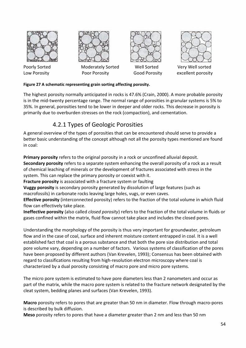
54

Poorly Sorted Moderately Sorted Well Sorted Very Well sorted Low Porosity Poor Porosity Good Porosity excellent porosity

Figure 27 A schematic representing grain sorting affecting porosity.

The highest porosity normally anticipated in rocks is 47.6% (Crain, 2000). A more probable porosity is in the mid-twenty percentage range. The normal range of porosities in granular systems is 5% to 35%. In general, porosities tend to be lower in deeper and older rocks. This decrease in porosity is primarily due to overburden stresses on the rock (compaction), and cementation.

4.2.1 Types of Geologic Porosities A general overview of the types of porosities that can be encountered should serve to provide a better basic understanding of the concept although not all the porosity types mentioned are found in coal: Primary porosity refers to the original porosity in a rock or unconfined alluvial deposit. Secondary porosity refers to a separate system enhancing the overall porosity of a rock as a result of chemical leaching of minerals or the development of fractures associated with stress in the system. This can replace the primary porosity or coexist with it. Fracture porosity is associated with a fracture system or faulting Vuggy porosity is secondary porosity generated by dissolution of large features (such as macrofossils) in carbonate rocks leaving large holes, vugs, or even caves. Effective porosity (interconnected porosity) refers to the fraction of the total volume in which fluid flow can effectively take place. Ineffective porosity (also called closed porosity) refers to the fraction of the total volume in fluids or gases confined within the matrix, fluid flow cannot take place and includes the closed pores. Understanding the morphology of the porosity is thus very important for groundwater, petroleum flow and in the case of coal, surface and inherent moisture content entrapped in coal. It is a well established fact that coal is a porous substance and that both the pore size distribution and total pore volume vary, depending on a number of factors. Various systems of classification of the pores have been proposed by different authors (Van Krevelen, 1993); Consensus has been obtained with regard to classifications resulting from high-resolution electron microscopy where coal is characterized by a dual porosity consisting of macro pore and micro pore systems. The micro pore system is estimated to have pore diameters less than 2 nanometers and occur as part of the matrix, while the macro pore system is related to the fracture network designated by the cleat system, bedding planes and surfaces (Van Krevelen, 1993). Macro porosity refers to pores that are greater than 50 nm in diameter. Flow through macro-pores is described by bulk diffusion. Meso porosity refers to pores that have a diameter greater than 2 nm and less than 50 nm

55

Micro porosity refers to pores that are smaller than 2 nm in diameter. Movement in micro-pores is by activated diffusion. Lower rank high volatile bituminous coals and sub bituminous coals have a relatively high total porosity and a high proportion of intermediate pore sizes. High rank bituminous coals have no intermediate sized pores and appreciably lower micro porosity, while lignite’s on the other hand have high levels of macro porosity.(Gan et al, 1972, Unsworth et al., 1989; Lamberson and Bustin, 1993; Levine 1993).

Figure 28 Relationship between coal porosity and coal rank (Gan, 1977, King and Wilkins, 1944 Levine, 1993)

Figure 28 above illustrates the effect of coal rank on porosity. Macro pores predominate in the lower ranks, while geophysical factors relating to compaction and water expulsion gradually reduce the porosity in the higher ranks. The development of secondary porosity begins with the formation of micro and meso pores at approximately the low volatile bituminous coal rank designation implying an increase in porosity due to progressive changes in the molecular structure through the higher ranks. Porosity is related to the maceral composition, where micro-porous content is found predominantly in the vitrinite content and meso to macro porous content predominates in inertinite (Gan et al, 1972, Unsworth et al., 1989; Lamberson and Bustin, 1993; Levine 1993). Coal porosity is also associated with cleats within the coal seams. Cleats are natural opening-mode fractures in coal beds. They usually occur in two sets that are, in most instances, mutually perpendicular and also perpendicular to bedding. These fracture sets, and partings along bedding planes, impart a blocky character to coal. Cleats account for the predominant natural porosity and permeability paths in coal seams. Coal cleats are extensional fractures that formed, especially in the

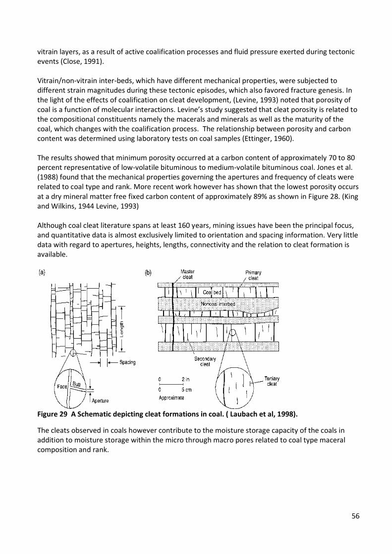
56

vitrain layers, as a result of active coalification processes and fluid pressure exerted during tectonic events (Close, 1991). Vitrain/non-vitrain inter-beds, which have different mechanical properties, were subjected to different strain magnitudes during these tectonic episodes, which also favored fracture genesis. In the light of the effects of coalification on cleat development, (Levine, 1993) noted that porosity of coal is a function of molecular interactions. Levine’s study suggested that cleat porosity is related to the compositional constituents namely the macerals and minerals as well as the maturity of the coal, which changes with the coalification process. The relationship between porosity and carbon content was determined using laboratory tests on coal samples (Ettinger, 1960). The results showed that minimum porosity occurred at a carbon content of approximately 70 to 80 percent representative of low-volatile bituminous to medium-volatile bituminous coal. Jones et al. (1988) found that the mechanical properties governing the apertures and frequency of cleats were related to coal type and rank. More recent work however has shown that the lowest porosity occurs at a dry mineral matter free fixed carbon content of approximately 89% as shown in Figure 28. (King and Wilkins, 1944 Levine, 1993) Although coal cleat literature spans at least 160 years, mining issues have been the principal focus, and quantitative data is almost exclusively limited to orientation and spacing information. Very little data with regard to apertures, heights, lengths, connectivity and the relation to cleat formation is available.

Figure 29 A Schematic depicting cleat formations in coal. ( Laubach et al, 1998).

The cleats observed in coals however contribute to the moisture storage capacity of the coals in addition to moisture storage within the micro through macro pores related to coal type maceral composition and rank.

57

Figure 30 Photograph of a 2.5m Mining Horizon section highlighting the nature of the face and formation of cleats on a macro scale.

Figure 31 Photograph of a hand sample also illustrating cleats especially noticeable in the vitrain layers of bright coal; note the blocky nature as a result of these smaller cleats.

One remarkable attribute of cleat formation is the extent to which they are developed in many coal beds of nearly all ranks in maturity. Cleats are typically much more closely spaced than fractures in adjacent non-coal rocks. Bright coal litho-types (vitrain) generally have smaller cleat spacing’s than dull coal litho-types (durain). Coals with low ash content tend to have smaller cleat spacing’s than coals with high ash content. Organic-rich shale’s also commonly have closely spaced fractures that resemble cleats. (Close, 1993)

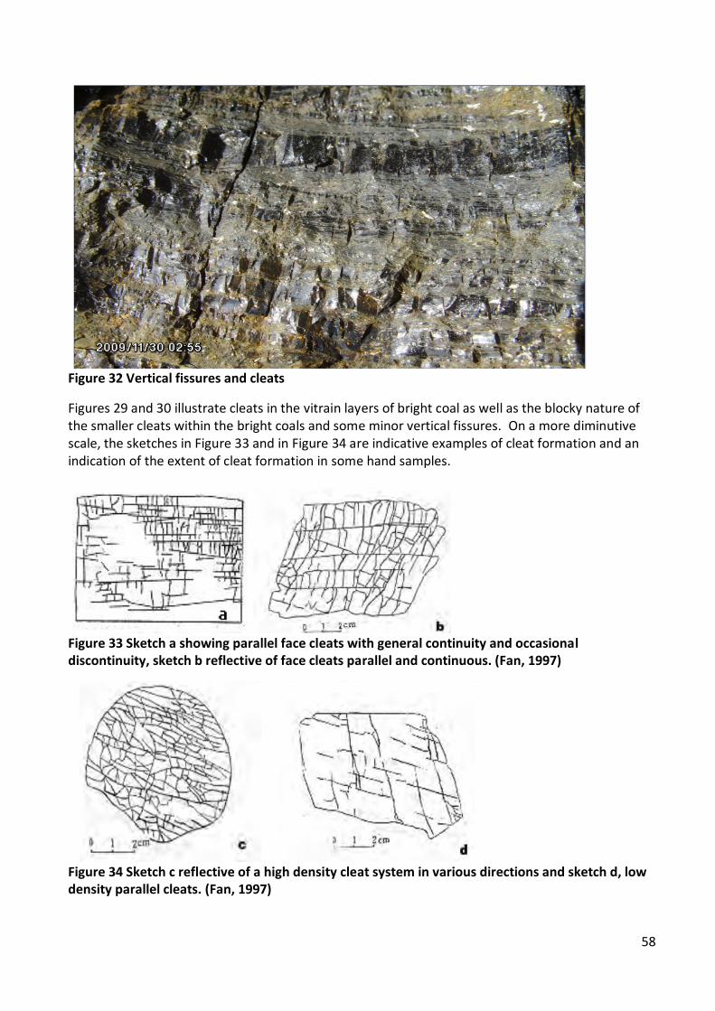
58

Figure 32 Vertical fissures and cleats

Figures 29 and 30 illustrate cleats in the vitrain layers of bright coal as well as the blocky nature of the smaller cleats within the bright coals and some minor vertical fissures. On a more diminutive scale, the sketches in Figure 33 and in Figure 34 are indicative examples of cleat formation and an indication of the extent of cleat formation in some hand samples.

Figure 33 Sketch a showing parallel face cleats with general continuity and occasional discontinuity, sketch b reflective of face cleats parallel and continuous. (Fan, 1997)

Figure 34 Sketch c reflective of a high density cleat system in various directions and sketch d, low density parallel cleats. (Fan, 1997)

59

It is evident that coal porosity and as such relative permeability can be highly variable. The movement or saturation by moisture would in many instances be by diffusion thus a reasonable amount of moisture would be retained in such a structure even if the large specimen were exposed to natural drying. This moisture is additional to the structurally bound moisture. An interesting study conducted by Xingjin Wang, (2007) during his research with relevance to the influence of coal quality factors on seam permeability associated with coal bed methane production and cleat studies illustrates the reality of the cleat formation perfectly. The emphasis of this study was focused on the major cleats and involved the reduction of coal core samples to 40mm cubes, which were treated with silicone gel in order to harden and preserve the samples. The cubes were then polished, removing the rough surfaces resulting in a smooth shining surface where the major cleats, spacing, length and apertures could be measured. The end result is portrayed in Figure 35. This was illustrative of the major cleats regarded as connective and providing a major contribution to seam permeability as well as contributing to increased porosity.

Figure 35 Photograph of a 40mm coal cube displaying the major cleats in filled with silicone to contrast against the coal background and also to strengthen and retain the coal sample intact. (Massorotto, 2003)

In summary, it is against the foregoing review that the research was undertaken as it is believed that every effort should be made to obtain the correct information with regard to the true density of coal in order to establish a realistic evaluation of a given coal deposit.

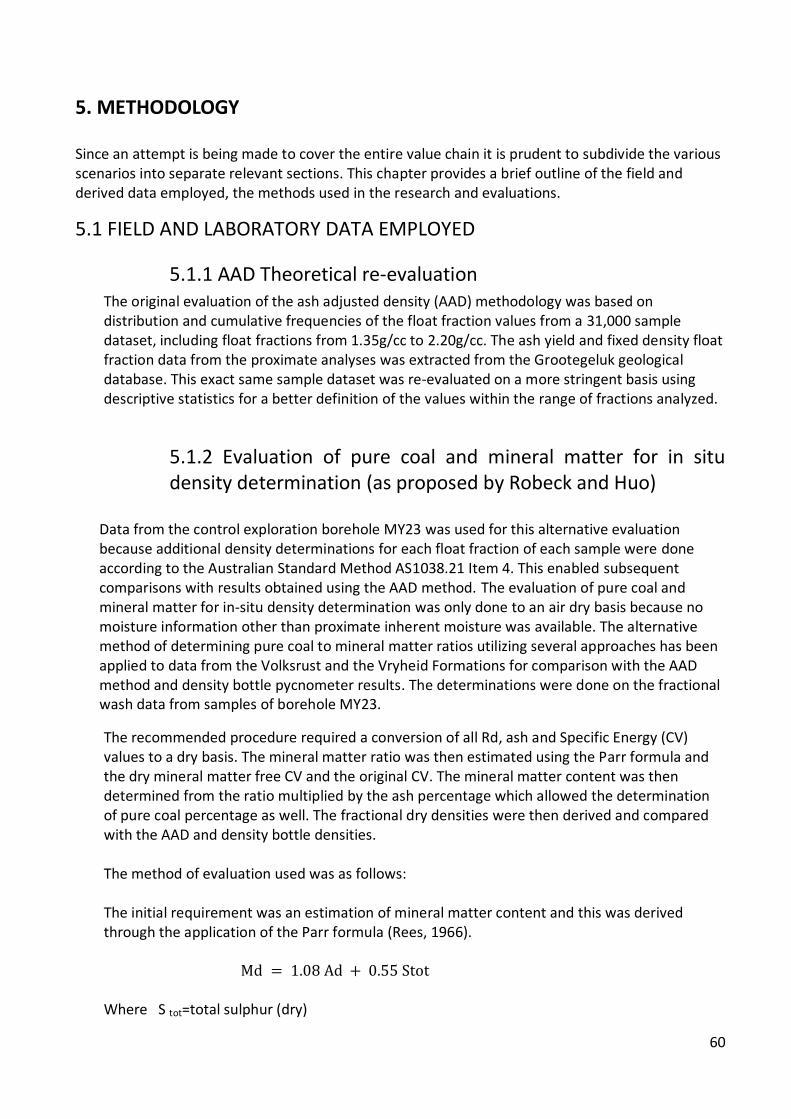
60

5. METHODOLOGY Since an attempt is being made to cover the entire value chain it is prudent to subdivide the various scenarios into separate relevant sections. This chapter provides a brief outline of the field and derived data employed, the methods used in the research and evaluations.

5.1 FIELD AND LABORATORY DATA EMPLOYED

5.1.1 AAD Theoretical re-evaluation The original evaluation of the ash adjusted density (AAD) methodology was based on distribution and cumulative frequencies of the float fraction values from a 31,000 sample dataset, including float fractions from 1.35g/cc to 2.20g/cc. The ash yield and fixed density float fraction data from the proximate analyses was extracted from the Grootegeluk geological database. This exact same sample dataset was re-evaluated on a more stringent basis using descriptive statistics for a better definition of the values within the range of fractions analyzed.

5.1.2 Evaluation of pure coal and mineral matter for in situ density determination (as proposed by Robeck and Huo)

Data from the control exploration borehole MY23 was used for this alternative evaluation because additional density determinations for each float fraction of each sample were done according to the Australian Standard Method AS1038.21 Item 4. This enabled subsequent comparisons with results obtained using the AAD method. The evaluation of pure coal and mineral matter for in-situ density determination was only done to an air dry basis because no moisture information other than proximate inherent moisture was available. The alternative method of determining pure coal to mineral matter ratios utilizing several approaches has been applied to data from the Volksrust and the Vryheid Formations for comparison with the AAD method and density bottle pycnometer results. The determinations were done on the fractional wash data from samples of borehole MY23.

The recommended procedure required a conversion of all Rd, ash and Specific Energy (CV) values to a dry basis. The mineral matter ratio was then estimated using the Parr formula and the dry mineral matter free CV and the original CV. The mineral matter content was then determined from the ratio multiplied by the ash percentage which allowed the determination of pure coal percentage as well. The fractional dry densities were then derived and compared with the AAD and density bottle densities. The method of evaluation used was as follows: The initial requirement was an estimation of mineral matter content and this was derived through the application of the Parr formula (Rees, 1966). Md = 1.08 Ad + 0.55 Stot Where S tot=total sulphur (dry)

61

And the mineral matter ratio was determined by

r = . .

An alternative, the Gray Method in which Md cannot exceed 100%, accounting for a wider range of mineral volatiles and revealing changes in mineral content with increasing ash only required specific energy (CV) and ash. This was the most robust, particularly for high ash samples. The relationship between dry CV and mineral matter was given by:

Ed = E dmmf100 − Md

100

Where Ed = Specific energy, dry expressed in MJ/Kg Edmmf =Specific energy, dry mineral matter free And the mineral matter ratio was determined by

r =100(Edmmf − Ed)

EdmmfAd

The dry mineral matter free CV was determined by:

Edmmf =100 ∗ (CV − 0.15S)

100 ∗ (Minh + 1.08) ∗ (Ad + 0.55S)

Mineral matter content was then derived by:

Md = rAd (For all samples, which implied all density fractions for each sample) The determination of the air dry density of the sample was then obtained from the equation:

ρest =100

(a + b) ∗ Md

Where coefficients a and b were determined by:

a =Minhρw + 100 −

Minhρc

Where ρc represents the matrix density of bituminous coal, 1.2384 g/cc and ρw was the density of water at 5ₒ degrees centigrade, 1.0 g/cc.

62

b = 100 −Minh100 ∗

ρc − ρmρc ∗ ρm

Where ρm = density of the mineral matter, here 2.53 g/cc was used for Waterberg coals. The samples individual densities were then obtained from the following equations.

ρc =100

a

And

ρm =100

a + (100 ∗ b)

The fractional dry densities were then derived and compared with the AAD and density bottle densities. An extracted sample showing the method applied to all samples in the evaluation using the method proposed by Robeck and Huo, 2015.

Table 4 an example of the analytical data per sample relevant to float/sink fractions their proximate analyses as well as swell, Roga and CV, for exploration borehole MY311LQ23

Table 5 an example of the calculated values used in the Gray method for the determination of relative density of the individual float fractions.

The spreadsheet columns in the calculated values for Gray method evaluation are as follows: Col 1, Fixed Carbon by deduction = 100-ash-volatiles-sulphur-moist Col 2, Dmmf = 100 (CV - 0.15Sulphur)/(100 - (Moist+1.08*Ash + 0.55Sulphur)) Col 3, Parr Ratio = ((1.08Ash) + (0.55Sulphur))/Ash Col 4, Gray Ratio = (Dmmf - CV)/(Dmmf * Ash/100)) Col 5, Mineral matter = Gray Ratio * Ash Col 6, Coal = 100 – Moist - Mineral matter

63

Col 7, Coefficient a = Moist + (100 – Moist/1.2384) Col 8, Coefficient b = ((100 – Moist/100) * ((1.2384 – 2.53)/(1.2384 * 2.53)) Col 9, Density Dry Coal = 100/Coefficient a Col 10, Density Mineral matter = 100/ (Coefficient a + (100 * Coefficient b)) Col 11, Fractional Density =( Coal * Density Dry Coal + Mineral Matter * Density Dry Mineral matter)/100

5.1.3 Detailed evaluation of sample float fractions from proximate analyses

The same sample set, which was used for the determination of the ash adjusted regression, was used in this detailed evaluation. The washability data, i.e. the fractional wash data for, individually, the coal and shale samples as well as composites of the coal and shale found in a delineated sample, combined with the associated proximate analyses were used to identify and typify the various types of coal found in the individual samples’ composition. A better evaluation of the overall properties of the samples can then be made. The introduction of a coal rank and type into this discussion and evaluation opens a whole new perspective in that a better understanding of its maceral composition, its maturation, metamorphic change in the basic structure and its matrix which can have an effect on the porosity and moisture holding capacity of the coal can be realized.

5.1.4 Ash adjusted density (AAD) Application in reconciliation of resources and reserves

This section deals with the evaluation and comparisons of the basic data obtained from field exploration boreholes and modelled information in a mining context. The entire process from sampling at the exploration drill site, initial sample preparation, field masses, field derived densities and preliminary relative density determinations are compared with laboratory results obtained for the respective samples from the selected boreholes. Composites of the defined mining horizons are compiled to obtain values representative of the entire representative mining bench and then compared with composites using the field obtained data.

Once the individual borehole composites with respect to their mining horizon delineation have been dealt with, the evaluation extends to modelled information relating to specific mining units in the specified mining horizons. Here the theoretical values as predicted can be compared with results from the actual mining operation. Tonnage differences between the datasets can then be used to determine the accuracy of the basic information with regard to primary densities and volumes used. This should assist in determining modifying factors to the original data.

64

5.1.5 Reserve and design (Information only - dealing with processes where the data is used in the value chain)

5.1.6 Planning and scheduling (Information only - dealing with processes where the data is used in the value chain)

5.1.7 Ash adjusted density (AAD) Application in product prediction and reconciliation of the beneficiation processes

Here a synopsis of previous work relevant to the Waterberg coals (Roux, 2012) in the beneficiation environment is given (refer to Chapter 8), since the findings led to the establishment of beneficiation plant specific correlation factors. These factors, however, still concealed underlying inexplicable reasons for their existence. The loss factors could not be categorized with respect to origin and cause and as such were seen as a compendium of errors based on reconciliation data. The focus in the evaluation in this thesis is now extended to include information relevant to moisture or effective porosity. The loss factors were applied to the budgeted run of mine tonnages over the monitoring period. [An assumption regarding these factors as being representative of moisture/porosity not accounted for in the derivation of the in-situ relative densities determined hydrostatically during exploration. Accepting these factors as being representative of moisture in the calculated budgeted run of mine tons derived from the original use of hydrostatically determined relative densities and applying them to the budgeted run of mine tonnages in order to compare derived tonnages with the actual reported tonnages, will clarify their origin]

5.1.8 Geological grade control and mining grade control through down-hole geophysical methods

In this section, an overview including the calibration of density (gamma gamma) probes, the evaluation of natural gamma logs and their general application in the established down-hole geophysical grade control system as devised and implemented by the author in the mid 1980’s are discussed. The most relevant fact recognized during the development and implementation of down-hole geophysical logging in grade control is that the geological personnel doing exploration, production or mining geology in the area must be conversant with the litho-types likely to be encountered and their identification via recognitive geophysical signatures and responses registered with the various down-hole tools used. As far as the down-hole geophysical equipment is concerned the absolute minimum requirement for reasonable lithological discrimination, correlation and determination of basic petrophysical properties in this area is, a Gamma-Gamma (density)/caliper probe, either dual density or short spaced single, as well as a large crystal natural gamma probe for high resolution and a single point resistivity and spontaneous potential probe. The original development work, refinements, implementation and use of the developed systems in various applications was not done in a systematic fashion, however research and refinement of all the methods, their various areas of application and data that can be derived for the geological grade control process has been structured logically

65

and formalized in acceptable procedures for the varied applications. As part of a major drive in utilizing all available information for the delineation of resources and reserves, it was decided that percussion drilled boreholes that had been geophysically logged, could be used for more than structural and Sedimentological verification on an in fill grid between existing exploration cored boreholes. Although the techniques and methodology have been in use for many years at Grootegeluk on a semi quantitative and semi qualitative basis in the production environment this has never been utilized for coal quality information that could supplement the overall resource and reserves values as well as the classifications of these. Chapter 7 in the “South African guide to systematic evaluation of coal resources and coal reserves “ SANS 10320:2004 refers to Evaluation methods and procedures and more specifically 7.3.3 refers to borehole down-hole geophysics where it is stated that primarily down hole geophysical surveys can be used to allow for stratigraphic correlation and core recovery calculations, coal seam roof and coal seam floor definition and overall lithological correlation, as well as being used for qualitative comparisons of coal quality in relation to proximal cored exploration boreholes. This is acceptable provided that, the calibrations are based on laboratory derived analysis and are comparable and reproducible with the geophysical responses measured and used for the derivation of the qualitative parameters. Should the criteria with respect to the reproducibility of the laboratory values compared with geophysically derived values within acceptable tolerances be met, these geophysically derived point values can then be utilized in improving the coal quality continuity required for certain classifications of the reserves. The crux of this application thus is to ensure that a proper calibration of the geophysical tool is obtained so that regressions obtained from analysis based on laboratory analysis of the various parameters can be applied for qualitative evaluation of the percussion drilled boreholes as well. The most logical place to start would then be at an exploration borehole, suitable for site specific calibration with laboratory and analytical data to validate the calibration accuracy. One of the exploration boreholes GK459LQ125 that has been used successively for calibration purposes was re-logged using the dual density/ natural gamma/ caliper tool after servicing and repairs by the manufacturer. The borehole was logged from its total depth to surface at a logging speed of approximately 3.0 m/minute, the original calibration data ignored and only raw counts per second for each 10cm interval logged over the entire sequence used. The geological log, sample intervals and coal and shale densities as well as their respective thicknesses were obtained from the Geological database. These values were then used in conjunction with the radiometric tool responses, raw counts per second data coupled to the sample intervals and density values allocated to averaged cps readings from the geological data so that regression analysis could be done to establish a calibration curve for the tool.

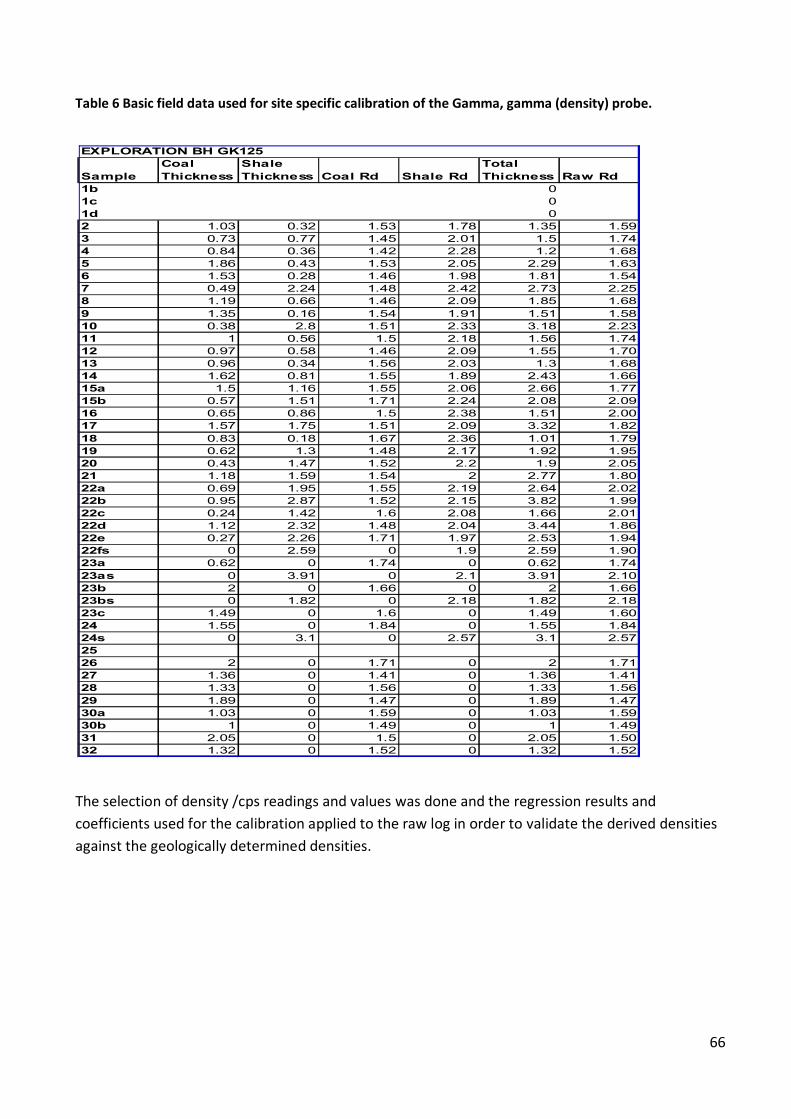
66

Table 6 Basic field data used for site specific calibration of the Gamma, gamma (density) probe.

The selection of density /cps readings and values was done and the regression results and coefficients used for the calibration applied to the raw log in order to validate the derived densities against the geologically determined densities.

EXPLORATION BH GK125

SampleCoal Thickness

Shale Thickness Coal Rd Shale Rd

Total Thickness Raw Rd

1b 0 1c 0 1d 0 2 1.03 0.32 1.53 1.78 1.35 1.593 0.73 0.77 1.45 2.01 1.5 1.744 0.84 0.36 1.42 2.28 1.2 1.685 1.86 0.43 1.53 2.05 2.29 1.636 1.53 0.28 1.46 1.98 1.81 1.547 0.49 2.24 1.48 2.42 2.73 2.258 1.19 0.66 1.46 2.09 1.85 1.689 1.35 0.16 1.54 1.91 1.51 1.5810 0.38 2.8 1.51 2.33 3.18 2.2311 1 0.56 1.5 2.18 1.56 1.7412 0.97 0.58 1.46 2.09 1.55 1.7013 0.96 0.34 1.56 2.03 1.3 1.6814 1.62 0.81 1.55 1.89 2.43 1.6615a 1.5 1.16 1.55 2.06 2.66 1.7715b 0.57 1.51 1.71 2.24 2.08 2.0916 0.65 0.86 1.5 2.38 1.51 2.0017 1.57 1.75 1.51 2.09 3.32 1.8218 0.83 0.18 1.67 2.36 1.01 1.7919 0.62 1.3 1.48 2.17 1.92 1.9520 0.43 1.47 1.52 2.2 1.9 2.0521 1.18 1.59 1.54 2 2.77 1.8022a 0.69 1.95 1.55 2.19 2.64 2.0222b 0.95 2.87 1.52 2.15 3.82 1.9922c 0.24 1.42 1.6 2.08 1.66 2.0122d 1.12 2.32 1.48 2.04 3.44 1.8622e 0.27 2.26 1.71 1.97 2.53 1.9422fs 0 2.59 0 1.9 2.59 1.9023a 0.62 0 1.74 0 0.62 1.7423as 0 3.91 0 2.1 3.91 2.1023b 2 0 1.66 0 2 1.6623bs 0 1.82 0 2.18 1.82 2.1823c 1.49 0 1.6 0 1.49 1.6024 1.55 0 1.84 0 1.55 1.8424s 0 3.1 0 2.57 3.1 2.5725 26 2 0 1.71 0 2 1.7127 1.36 0 1.41 0 1.36 1.4128 1.33 0 1.56 0 1.33 1.5629 1.89 0 1.47 0 1.89 1.4730a 1.03 0 1.59 0 1.03 1.5930b 1 0 1.49 0 1 1.4931 2.05 0 1.5 0 2.05 1.5032 1.32 0 1.52 0 1.32 1.52

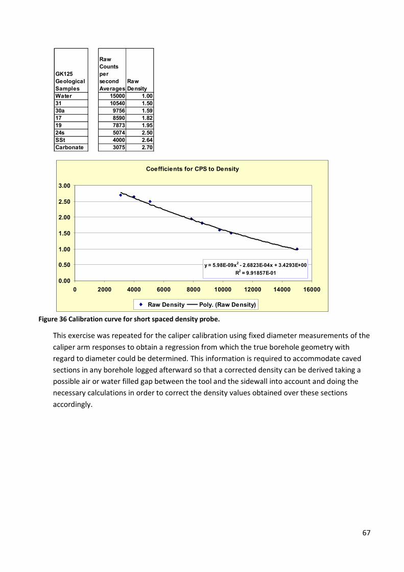
67

Figure 36 Calibration curve for short spaced density probe.

This exercise was repeated for the caliper calibration using fixed diameter measurements of the caliper arm responses to obtain a regression from which the true borehole geometry with regard to diameter could be determined. This information is required to accommodate caved sections in any borehole logged afterward so that a corrected density can be derived taking a possible air or water filled gap between the tool and the sidewall into account and doing the necessary calculations in order to correct the density values obtained over these sections accordingly.

GK125 Geological Samples

Raw Counts per second Averages

Raw Density

Water 15000 1.0031 10540 1.5030a 9756 1.5917 8590 1.8219 7873 1.9524s 5074 2.50SSt 4000 2.64Carbonate 3075 2.70

Coefficients for CPS to Density

y = 5.98E-09x2 - 2.6823E-04x + 3.4293E+00R2 = 9.91857E-01

0.00

0.50

1.00

1.50

2.00

2.50

3.00

0 2000 4000 6000 8000 10000 12000 14000 16000

Raw Density Poly. (Raw Density)

68

Figure 37 Caliper arm calibration data and curve with coefficients.

Having completed the calibration, the coefficients derived were used to determine geophysical log derived densities for the entire log, densities relevant to the defined samples were then derived from intervals representative of the respective samples and tabulated. Correlations between geophysically derived values and the raw densities for the respective samples were then done and the results are summarized in Table 7 below. A further validation of this calibration has been done by determining core recovery from the calculated masses of the samples against the field masses and then determining the corrected density using the core recovery value. Correlations between these values and geophysically derived values are shown in Table 8. Both datasets Tables 7 & 8 giving good correlations above a 95% confidence level, which thus implies that the coefficients can be used to determine the in-situ densities of the lithological strata from the geophysical logs. The geophysical logs can further be used for lithological definition, sample delineation, roof and floor definition, as well as cross correlation between percussion drilled and cored boreholes allowing structural definition along a section of adjacent boreholes, which adds value to the structural delineation of mining horizons used for structural modelling.

CPS Width mm

990 140766 100487 50

Caliper Arm Calibration

y = 0.1789x - 37.119R2 = 1

0

20

40

60

80

100

120

140

160

0 200 400 600 800 1000 1200

Width mmPoly. (Width mm)

69

Table 7 Correlation of geophysically derived Rd's using calibration coefficients against raw Rd data.

SampleDepth From

Depth to ST

RA

TIG

RA

PHY

Raw Density from sampling

Logged Density

Sample Rd Correlations

Bench Rd values and correlations

2 15.31 16.66 1.59 1.64 1033 16.66 18.16 1.74 1.73 1004 18.16 19.36 1.68 1.66 995 19.36 21.65 1.63 1.62 1006 21.65 23.46 1.54 1.56 1017 23.46 26.19 2.25 2.17 968 26.19 28.04 1.68 1.69 1009 28.04 29.55 1.58 1.64 10410 29.55 32.73 2.23 2.14 9611 32.73 34.29 1.74 1.74 10012 34.29 35.84 1.70 1.73 10213 35.84 37.14 1.68 1.68 10014 37.14 39.57 1.66 1.67 10015a 39.57 42.23 1.77 1.79 10115b 42.23 44.31 2.09 2.05 9816 44.31 45.82 2.00 1.96 9817 45.82 49.14 1.82 1.87 10318 49.14 50.15 1.79 1.99 11119 50.15 52.07 1.95 1.98 10220 52.07 53.99 2.05 2.01 9821 53.99 56.76 1.80 1.83 10122a 56.76 59.4 2.02 2.03 10022b 59.4 63.22 1.99 2.00 10022c 63.22 64.88 2.01 2.03 10122d 64.88 68.32 1.86 1.88 10122e 68.32 70.85 1.94 1.97 10122fs 70.85 73.44 1.90 1.90 10023a 73.44 74.06 1.74 1.79 10323b 74.06 76.06 1.66 1.69 10223c 76.06 77.55 1.60 1.66 10423as 77.55 81.46 2.10 2.06 9823bs 81.46 83.28 2.18 2.14 98

24 83.28 84.83 1.84 1.90 103

Bench 7B Raw Rd 1.84g/cc Geophys Rd 1.90g/cc correlation 103.2%

24s 84.83 87.93 2.57 2.41 94 Interbeds26 87.93 89.93 1.71 1.72 10127 89.93 91.29 1.41 1.51 10728 91.29 92.62 1.56 1.58 10129 92.62 94.51 1.47 1.56 10630a 100.72 101.8 1.59 1.63 10330b 101.75 102.9 1.49 1.50 10131 102.88 104.8 1.50 1.52 101

32 117.37 118.7 1.52 1.54 101Bench 13 correlation 101.3%

Bench 11 Raw Rd 1.54g/cc Geophys Rd 1.57g/cc correlation

Tran

sitio

nVR

YHEI

D F

OR

MA

TIO

N

Bench 3 Geol Raw Rd 1.82g/cc geophys Rd 1.81g/cc correlation

99.45%

Bench 4 Geol Raw Rd 1.91g/cc geophys Rd 1.94g/cc correlation

101.57%

Bench 5 Geol Raw Rd 1.95g/cc Geophys Rd 1.97g/cc correlation

101.02%

Bench 2 Geol Raw Rd 1.63g/cc geophys Rd 1.64g/cc correlation

100.61%

EXPLORATION BOREHOLE GK459LQ 125

Bench 6 Raw Rd 1.67g/cc Geophys Rd 1.71g/cc

correlation 103%

Bench 9 Raw Rd 1.54g/cc Geophys Rd 1.59g/cc correlation 103.25%

Interbeds

70

Table 8 Correlation between geophysically derived Rd's and corrected sample Rd's derived from core recovery calculations.

The regression evaluation of densities derived from the application of determined algorithm on a reverse compatibility test shown Figure 38 gives a very good correlation as indicated by the regression results.

SampleDepth From

Depth to ST

RA

TIG

RAPH

Y

Raw Density from sampling

Logged Density

Sample Rd Correlations

Bench Rd values and correlations

Core Recovery

Adj Raw Density based on core recovery

Adjusted correlation between log desity and corrected Raw density

2 15.31 16.66 1.59 1.64 103 93.67 1.70 973 16.66 18.16 1.74 1.73 100 94.77 1.83 944 18.16 19.36 1.68 1.66 99 92.39 1.82 915 19.36 21.65 1.63 1.62 100 94.70 1.72 946 21.65 23.46 1.54 1.56 101 94.05 1.64 957 23.46 26.19 2.25 2.17 96 96.96 2.32 938 26.19 28.04 1.68 1.69 100 96.77 1.74 979 28.04 29.55 1.58 1.64 104 97.23 1.62 101

10 29.55 32.73 2.23 2.14 96 97.99 2.28 9411 32.73 34.29 1.74 1.74 100 97.59 1.79 9712 34.29 35.84 1.70 1.73 102 97.15 1.75 9913 35.84 37.14 1.68 1.68 100 98.75 1.70 9914 37.14 39.57 1.66 1.67 100 96.73 1.72 9715a 39.57 42.23 1.77 1.79 101 94.81 1.87 9615b 42.23 44.31 2.09 2.05 98 97.21 2.15 9516 44.31 45.82 2.00 1.96 98 97.47 2.05 9517 45.82 49.14 1.82 1.87 103 98.12 1.85 10118 49.14 50.15 1.79 1.99 111 95.89 1.87 10619 50.15 52.07 1.95 1.98 102 97.20 2.00 9920 52.07 53.99 2.05 2.01 98 97.64 2.10 9621 53.99 56.76 1.80 1.83 101 97.98 1.84 9922a 56.76 59.4 2.02 2.03 100 98.56 2.05 9922b 59.4 63.22 1.99 2.00 100 96.50 2.07 9722c 63.22 64.88 2.01 2.03 101 98.63 2.04 10022d 64.88 68.32 1.86 1.88 101 98.87 1.88 10022e 68.32 70.85 1.94 1.97 101 97.06 2.00 9822fs 70.85 73.44 1.90 1.90 100 96.55 1.97 9723a 73.44 74.06 1.74 1.79 103 99.94 1.74 10323b 74.06 76.06 1.66 1.69 102 97.11 1.71 9923c 76.06 77.55 1.60 1.66 104 99.13 1.61 103

23as 77.55 81.46 2.10 2.06 98 98.06 2.14 9623bs 81.46 83.28 2.18 2.14 98 98.41 2.22 97

24 83.28 84.83 1.84 1.90 103

Bench 7B Raw Rd 1.84g/cc Geophys Rd 1.90g/cc correlation

103.2%

97.92 1.88 101

24s 84.83 87.93 2.57 2.41 94 Interbeds 98.82 2.60 9326 87.93 89.93 1.71 1.72 101 96.64 1.77 9727 89.93 91.29 1.41 1.51 107 93.74 1.50 10028 91.29 92.62 1.56 1.58 101 98.61 1.58 10029 92.62 94.51 1.47 1.56 106 97.19 1.51 10330a 100.72 101.8 1.59 1.63 103 95.51 1.66 9830b 101.75 102.9 1.49 1.50 101 96.26 1.55 9731 102.88 104.8 1.50 1.52 101 96.10 1.56 97

32 117.37 118.7 1.52 1.54 101 Bench 13 correlation 101.3% 99.09 1.53 100

Bench 11 Raw Rd 1.54g/cc Geophys Rd 1.57g/cc correlation

VOLK

SRU

ST F

ORM

ATI

ON

Tran

sitio

nVR

YHEI

D F

OR

MA

TIO

N

Bench 3 Geol Raw Rd 1.82g/cc geophys Rd 1.81g/cc correlation

99.45%

Bench 4 Geol Raw Rd 1.91g/cc geophys Rd 1.94g/cc correlation

101.57%

Bench 5 Geol Raw Rd 1.95g/cc Geophys Rd 1.97g/cc correlation

101.02%

Bench 2 Geol Raw Rd 1.63g/cc geophys Rd 1.64g/cc correlation

100.61%

EXPLORATION BOREHOLE GK459LQ 125

Bench 6 Raw Rd 1.67g/cc Geophys Rd 1.71g/cc

correlation 103%

Bench 9 Raw Rd 1.54g/cc Geophys Rd 1.59g/cc correlation 103.25%

Interbeds

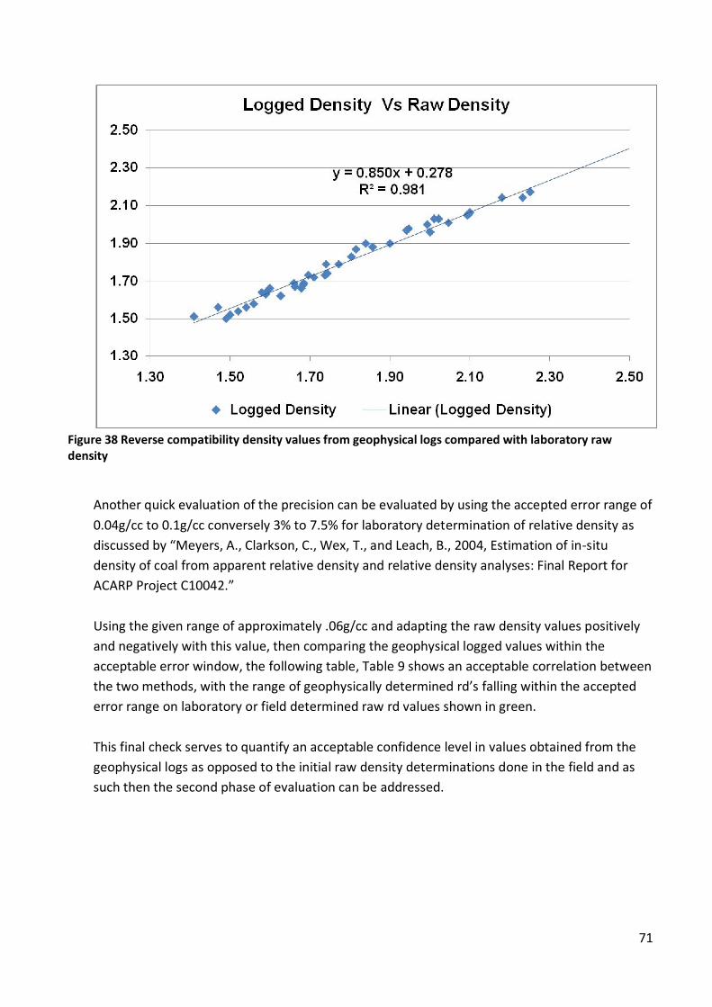
71

Figure 38 Reverse compatibility density values from geophysical logs compared with laboratory raw density

Another quick evaluation of the precision can be evaluated by using the accepted error range of 0.04g/cc to 0.1g/cc conversely 3% to 7.5% for laboratory determination of relative density as discussed by “Meyers, A., Clarkson, C., Wex, T., and Leach, B., 2004, Estimation of in-situ density of coal from apparent relative density and relative density analyses: Final Report for ACARP Project C10042.” Using the given range of approximately .06g/cc and adapting the raw density values positively and negatively with this value, then comparing the geophysical logged values within the acceptable error window, the following table, Table 9 shows an acceptable correlation between the two methods, with the range of geophysically determined rd’s falling within the accepted error range on laboratory or field determined raw rd values shown in green. This final check serves to quantify an acceptable confidence level in values obtained from the geophysical logs as opposed to the initial raw density determinations done in the field and as such then the second phase of evaluation can be addressed.

72

Table 9 geophysically determined densities within the accepted error range on laboratory determined density precision.

The method applied in evaluating the geophysical data and relating this to laboratory data was extended to incorporate the evaluation of a petrophysical matrix density (The physical characteristics of the matrix) for the material being mined. This petrophysical matrix density compared with the bulk relative density derived from a short spaced density log is used to determine effective porosity or moisture content at the time of logging. The moisture holding capacity or effective porosity value, used in conjunction with the true absolute dry density, was applied in order to obtain a better approximation of the density values used for the conversion of volumes to tonnages required for the various sub divisions of resource and reserve tonnage estimations.

Sample Depth From Depth to STRA

TIG

RAP

HY Raw Density

from sampling

Logged Density

Bench Rd values and correlations

Core Recovery

2 15.31 16.66 1.59 1.64 93.67 1.65 1.533 16.66 18.16 1.74 1.73 94.77 1.80 1.684 18.16 19.36 1.68 1.66 92.39 1.74 1.625 19.36 21.65 1.63 1.62 94.70 1.69 1.576 21.65 23.46 1.54 1.56 94.05 1.60 1.487 23.46 26.19 2.25 2.17 96.96 2.31 2.198 26.19 28.04 1.68 1.69 96.77 1.74 1.629 28.04 29.55 1.58 1.64 97.23 1.64 1.52

10 29.55 32.73 2.23 2.14 97.99 2.29 2.1711 32.73 34.29 1.74 1.74 97.59 1.80 1.6812 34.29 35.84 1.70 1.73 97.15 1.76 1.6413 35.84 37.14 1.68 1.68 98.75 1.74 1.6214 37.14 39.57 1.66 1.67 96.73 1.72 1.6015a 39.57 42.23 1.77 1.79 94.81 1.83 1.7115b 42.23 44.31 2.09 2.05 97.21 2.15 2.0316 44.31 45.82 2.00 1.96 97.47 2.06 1.9417 45.82 49.14 1.82 1.87 98.12 1.88 1.7618 49.14 50.15 1.79 1.99 95.89 1.85 1.7319 50.15 52.07 1.95 1.98 97.20 2.01 1.8920 52.07 53.99 2.05 2.01 97.64 2.11 1.9921 53.99 56.76 1.80 1.83 97.98 1.86 1.7422a 56.76 59.4 2.02 2.03 98.56 2.08 1.9622b 59.4 63.22 1.99 2.00 96.50 2.05 1.9322c 63.22 64.88 2.01 2.03 98.63 2.07 1.9522d 64.88 68.32 1.86 1.88 98.87 1.92 1.8022e 68.32 70.85 1.94 1.97 97.06 2.00 1.8822fs 70.85 73.44 1.90 1.90 96.55 1.96 1.8423a 73.44 74.06 1.74 1.79 99.94 1.80 1.6823b 74.06 76.06 1.66 1.69 97.11 1.72 1.60

23c 76.06 77.55 1.60 1.66 99.13 1.66 1.54

23as 77.55 81.46 2.10 2.06 98.06 2.16 2.0423bs 81.46 83.28 2.18 2.14 98.41 2.24 2.12

24 83.28 84.83 1.84 1.90Bench 7B Raw Rd 1.84g/cc

Geophys Rd 1.90g/cc correlation 103.2%

97.92 1.90 1.78

24s 84.83 87.93 2.57 2.41 Interbeds 98.82 2.63 2.5126 87.93 89.93 1.71 1.72 96.64 1.77 1.6527 89.93 91.29 1.41 1.51 93.74 1.47 1.3528 91.29 92.62 1.56 1.58 98.61 1.62 1.5029 92.62 94.51 1.47 1.56 97.19 1.53 1.4130a 100.72 101.75 1.59 1.63 95.51 1.65 1.5330b 101.75 102.88 1.49 1.50 96.26 1.55 1.4331 102.88 104.8 1.50 1.52 96.10 1.56 1.44

32 117.37 118.69 1.52 1.54 Bench 13 correlation 101.3% 99.09 1.58 1.46

Bench 9 Raw Rd 1.54g/cc Geophys Rd 1.59g/cc correlation 103.25%

Bench 11 Raw Rd 1.54g/cc Geophys Rd 1.57g/cc correlation 101.95%

Acceptable error Range of 0.06g/cc precision based on

raw density pre-determined

Tran

sitio

n

Bench 5 Geol Raw Rd 1.95g/cc Geophys Rd

1.97g/cc correlation 101.02%

Bench 6 Raw Rd 1.67g/cc Geophys Rd 1.71g/cc

correlation 103%

Interbeds

Bench 2 Geol Raw Rd 1.63g/cc geophys Rd

1.64g/cc correlation 100.61%

Bench 3 Geol Raw Rd 1.82g/cc geophys Rd

1.81g/cc correlation 99.45%

Bench 4 Geol Raw Rd 1.91g/cc geophys Rd

1.94g/cc correlation 101.57%

VOLK

SRU

ST F

OR

MA

TIO

NVR

YHEI

D F

ORM

ATI

ON

73

6 RESEARCH AND EVALUATION RESULTS The results of the various methods listed in Chapter 5 are presented in this Chapter.

6.1.1 AAD Theoretical Re-Evaluation. The original theory with regard to the ash adjusted density (AAD) methodology as published in “OPTIMAL YIELD AND CUT DENSITY PREDICTION OF SEMI SOFT COKING COAL AND POWERSTATION COAL IN THE WATERBERG COALFIELD, LIMPOPO PROVINCE.” by Roux (2012) was based on distribution and cumulative frequencies of the float fraction density and ash values from a 31,000 sample dataset. These values were used to determine the regression trends between ash and float sink densities. Plots of these regressions were compared to composite plots of other mining unit compositions as well as samples that had been washed at lower float densities than the norm. The evaluation produced three sets of regression data for density against ash which were in extremely close proximity with regard to their R2 values and the linear trends were almost identical. The equations derived are repeated in this research as a base line reference to indicate the relative changes and improvements that have now been achieved resulting from the re-evaluation of the original dataset Linear regressions for Ash/Density R-Fit

a) 0.0136 x Ash + 1.198 0.999 b) 0.0136 x Ash + 1.1994 0.9926 c) 0.0136 x Ash + 1.2018 0.9973

The re-evaluation of the sample dataset was accomplished by doing descriptive statistics for each sample float fraction and doing regressions on the mean, median and mode ash values for the representative float fractions, to complement and enhance the original ash, density regressions done on the dataset. The re-evaluated statistics for the ash content at the coal float fractions are presented in Table 10 Descriptive statistics results for the float fractions in the ranges 0-1.35g/cc, 1.35g/cc – 1,40g/cc thru to a final float fraction at 2.10g/cc analyzed.

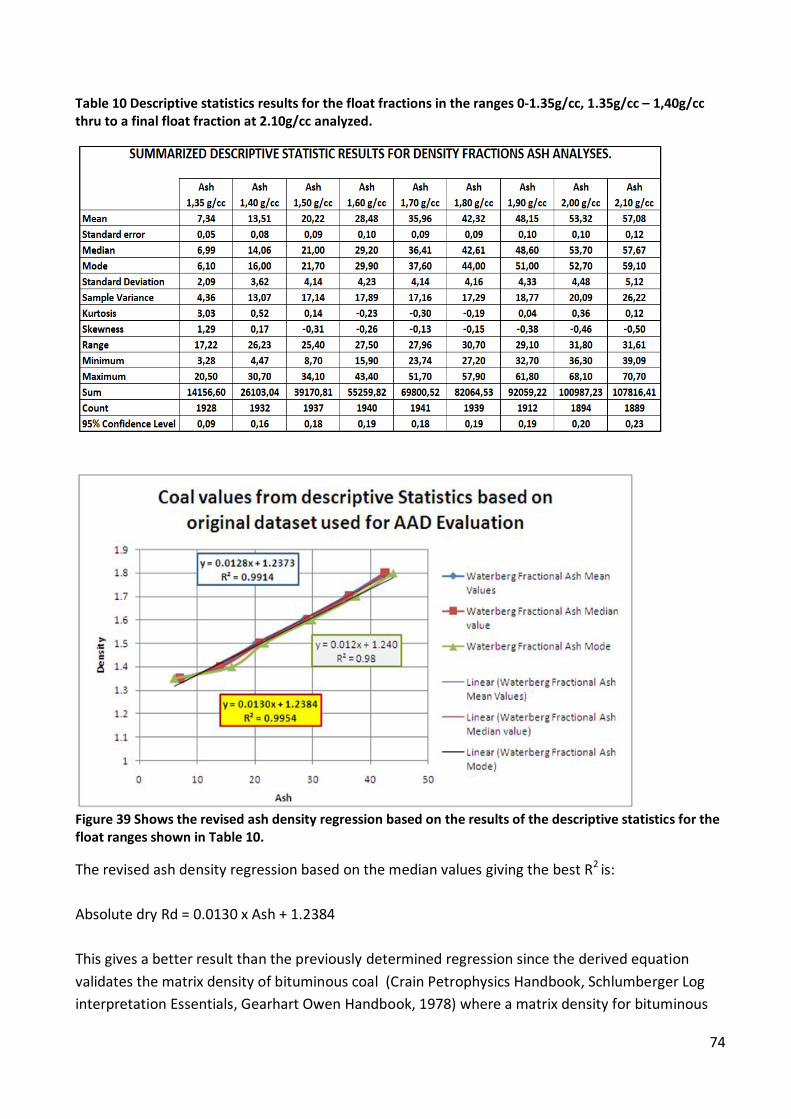
74

Table 10 Descriptive statistics results for the float fractions in the ranges 0-1.35g/cc, 1.35g/cc – 1,40g/cc thru to a final float fraction at 2.10g/cc analyzed.

Figure 39 Shows the revised ash density regression based on the results of the descriptive statistics for the float ranges shown in Table 10.

The revised ash density regression based on the median values giving the best R2 is: Absolute dry Rd = 0.0130 x Ash + 1.2384 This gives a better result than the previously determined regression since the derived equation validates the matrix density of bituminous coal (Crain Petrophysics Handbook, Schlumberger Log interpretation Essentials, Gearhart Owen Handbook, 1978) where a matrix density for bituminous

75

coal is given as 1.24 g/cc, for anthracite 1.47 g/cc and lignite 1.19 g/cc. The first part of the equation represents the incremental indestructible mineral content of the sample with the intercept being represented by a constant equivalent to the matrix density of a bituminous coal. The earlier evaluation’s regression appears to fit a matrix density for Lignite, in that Rd = 0.0136 x Ash + 1.198 The ash adjusted density value represents the absolute dry density of the float fraction. An approximation of the expected air dry density was made using the inherent moisture content derived from proximate analysis. The resultant density value was found to be slightly higher than the AAD value determined. A reconstruction of the sample to in situ relative density could then be calculated, provided that the free moisture content and air or gas filled voids of an impeccably preserved sample are known. Table 11 Sample 1A from borehole MY311LQ23 fixed density yield fractions evaluated using both sets of equations for AAD dry density values, also densities after the adjustment taking inherent moisture into account to represent an air dry density for the fractional values.

6.1.2 Ash Adjusted Density Validated Against Laboratory Determined Density

An exploration borehole was sampled according to a rigid procedure established to ensure that the same strata would always be represented by the same sample number from borehole to borehole. The individual samples represent the subdivision of the coal zones into smaller sub-cycles that could be correlated confidently from borehole to borehole ensuring correct stratigraphic correlation which is of prime importance in a multi-seam coal deposit such as the Waterberg coalfield. A full succession borehole, starting in the Volksrust formation with coal zone 11 uppermost and ending in the Vryheid Formation at coal zone 1, contains 75 samples i.e. 42 coal samples and 33 shale samples. After the drilled core has been sampled the relative density of each sample was determined in the field. Core recovery according to the stipulated procedure was then calculated from the mass, relative density and the core diameter. The field mass i.e. mass in air was then expressed as a percentage of the calculated mass derived from the relative density and the volume

76

of drill core, which purportedly represented the core recovery. The samples were then dispatched for analysis to an accredited laboratory. Here the samples were crushed to -13mm and screened at 0.5mm, they were then floated at relative densities from 1.35 g/cc through 2.20g/cc and by special request the true relative density of each float fraction was determined using the density bottle method at the same laboratory. Thereafter analyses pertinent to stipulations referring to analysis to be done on the Volksrust formation (samples 1A through 22E) such as Proximate, FSI, Roga, Sulphur, CV, Petrography, Ash analysis and Ash fusion and stipulations for analysis of the Vryheid Formation samples (23A to 32) were performed. The -0.5mm fraction of all samples was treated as a raw sample with only Proximate, Sulphur and CV done on these. These values were compared with ash adjusted density values obtained through the application of the derived algorithm to ascertain the accuracy of said algorithm. A total of 1014 float and sink fraction’s “true relative densities” were determined. The relative density values were determined according to the Australian Standard method, “AS1038.21 Item 4”. This is the most common method of determining coal density. Whilst the method is cheap and easy to apply, the state of the sample, when tested, does not simulate the in-situ condition of the coal. The sample is: • Ground to-212\µm size, thereby removing fissures and some pores • Air-dried i.e. retaining some, but not all of, its in-situ moisture. The method involves measuring the amount of liquid displaced by the coal, either in a density bottle or in a volumetric flask, and hence determining its volume. This is then related to the original weighed mass. The major problem with the method is the inability of the liquid (either water or wetting agent under vacuum, or methylated spirits) to occupy all pores within the coal i.e. to displace all air and water. The result gives neither absolute relative density nor in-situ relative density. However it probably approaches the former more closely than the latter. For example, experiments carried out by Ettinger and Zhupakhina (1981) compared the results obtained for coal using the density bottle and helium porosimetry methods. In the former test, the coal was ground more finely than usual, and the water and wetting agent boiled to facilitate pore penetration. Agreement between the methods was excellent, for a wide range of coal types and ranks. Thus, under certain rigorously controlled conditions, the Standard Density bottle method may give results closely approximating the "true" or absolute relative density for coal (expressed on the air-dry basis).

In this entire process of converting a coal sample to a ground, air dried state the greatest change was noted in the volume, which has a greater effect on the relative density than the loss of mass. The core samples were originally crushed to -13mm and screened to 0.5mm, they were then ground to -212 µm for the density bottle testing. In this situation, the density trend would approximate the absolute density of the coal. The float and sink wash data for the exploration borehole MY311LQ23 was evaluated. The two main stratigraphic units in that borehole were separated for this evaluation and the wash data presented in the figures below. The Volksrust Formation coal samples contain minor shale lenses included in the sample due to the nature of the deposit being an intercalated

77

coal and shale sequence (this is often referred to as a bar-coded sequence). Figure 40 displays the ash values obtained from the Volksrust Formation for individual fractions that floated at the specific density range depicted. The ash values are indicative of a range of values related to minor differences in the relative density of the individual fractions.

Figure 40 Volksrust Formation coal sample ash content from wash data as primarily obtained at fixed density cut points from laboratory analyses.

The ash adjusted density theory, as proven by Roux (2012), provides an adjustment of each sample to reflect its absolute dry density. This rearranges the density/ ash values which then conform to the trend previously established (Roux L. 2010). Figure 40 is a plot of the re-determined, true relative densities of the individual samples as determined by an accredited laboratory according to the Australian Standard “AS1038.21 Item 4”. A 4th order polynomial regression of this data gives an R2 value of 0.9652. The slight differences may be attributable to changes in the porosity of the coal. These discrepancies have been mentioned earlier in regard to the method applied in the determination of the relative density. The sample is ground to -212µm, removing fissures and some of the pores, and is then air dried, retaining some of its in situ or as received moisture. This is due to the fact that many of the pores are much finer than the particles, thus a fair amount of porosity could be retained.

78

Figure 41 Re-determined relative density values for the respective float fractions of the same borehole in the Volksrust Formation.

The same approach was applied to the Vryheid Formation coals. These coals are discreet beds or seams of relatively pure coal material separated by siltstone and sandstone inter-beds.

Figure 42 Vryheid Formation coal sample wash data as primarily obtained at fixed density cut points.

Figure 41 portraying the float and sink data for the Vryheid Formation samples indicates narrower range of ash percentage data per float fraction than the same range portrayed in the Volksrust Formation in Figure 39. It is notable that the ash percentage ranges at each density fraction are

79

much smaller, ranging in the lower density values from a 5 percent total ash to a maximum of approximately 12 percent at the 2.20g/cc fixed density cut point.

Figure 43 Re-determined relative density values for the respective float fractions of the same borehole Vryheid Formation.

Using all the samples, i.e. coal and shale combined, and comparing the differences between the AAD derived densities and the re-determined laboratory densities, with a normal distribution evaluation at a 99.9% confidence level, has revealed that the cumulative probability of the difference between the two measured datasets is minor which shows a very positive result. The values obtained for the re-determined densities are portrayed in Figure 44 where the re-determined values as well as the AAD densities are plotted against the ash% obtained from the proximate analyses of the float fractions. Comparisons of the two sets of results I.e. laboratory density bottle determined RD and AAD RD values were found to be very close. The standard deviation based on the differences between the re-determined density bottle RD and the AAD RD is 0.08.

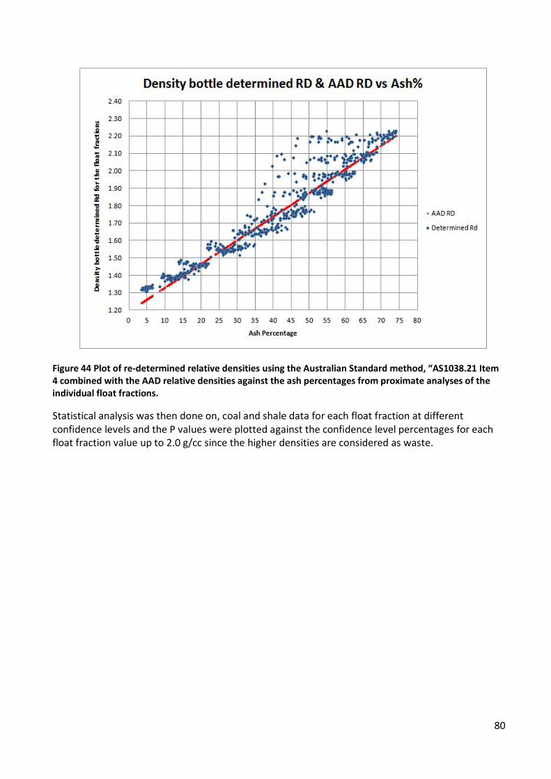
80

Figure 44 Plot of re-determined relative densities using the Australian Standard method, “AS1038.21 Item 4 combined with the AAD relative densities against the ash percentages from proximate analyses of the individual float fractions.

Statistical analysis was then done on, coal and shale data for each float fraction at different confidence levels and the P values were plotted against the confidence level percentages for each float fraction value up to 2.0 g/cc since the higher densities are considered as waste.

81

The results are shown in Figure 45. Thereafter the same was done for coal, shale and a combination of both. The results are shown in Figure 46.

Figure 45 Plot of P values for confidence levels rangng from 50% to 99.9% for each evaluated float fraction.

A plot of p values obtained at confidence levels ranging from 50% through to 99.9% for separate coal and shale as well as combined coal and shale samples are higher than a 95% confidence level. The shale p value however does not conform to a 99.9% confidence level. This is shown in Figure 46. The last three sets of values obtained at the various confidence levels indicate a high level of accuracy. Since this evaluation is based on a comparison between AAD calculated values and laboratory determined values, it is apparent that the AAD methodology can be implemented and used confidently for predictions of air dry densities in coal assessments.

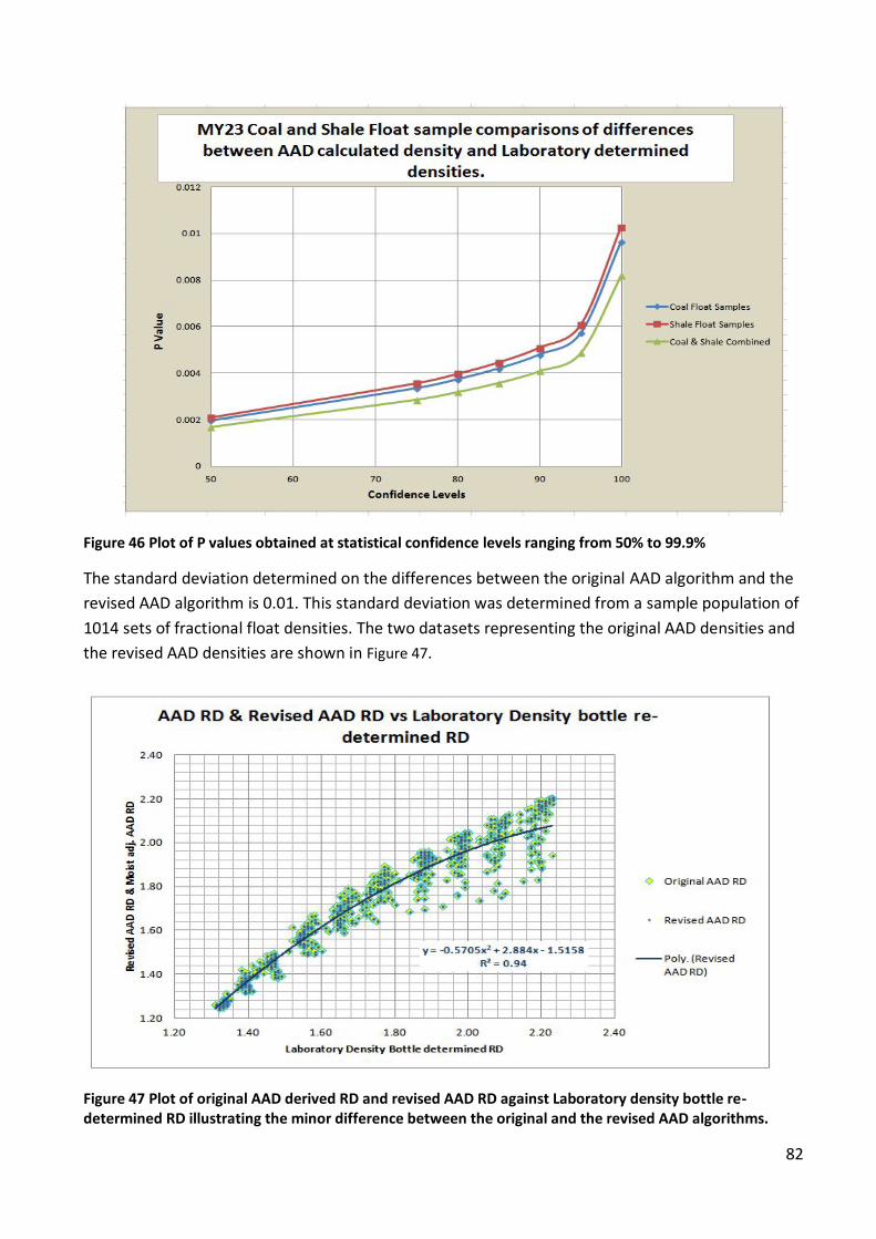
82

Figure 46 Plot of P values obtained at statistical confidence levels ranging from 50% to 99.9%

The standard deviation determined on the differences between the original AAD algorithm and the revised AAD algorithm is 0.01. This standard deviation was determined from a sample population of 1014 sets of fractional float densities. The two datasets representing the original AAD densities and the revised AAD densities are shown in Figure 47.

Figure 47 Plot of original AAD derived RD and revised AAD RD against Laboratory density bottle re-determined RD illustrating the minor difference between the original and the revised AAD algorithms.

83

In summary, this research was confined to the crushed, air dried -13mm+0.5mm material that was sink/floated to obtain a range of fractions for further analysis. The values pertinent to the true density of the matrix material have been assessed via re-determination of relative density and alteration of the ash adjusted density algorithm and then compared. The fractional portions of the samples now need to be reconstructed through a cumulating process to obtain the overall relative density of the whole sample. The density value thus obtained would then be representative of the true or absolute relative density of the combined solid matrix materials. I.e. the samples need to be reconstructed to resemble the in situ raw material prior to crushing. Restoration of the sample to its original volume is required. This was achieved by considering properties such as moisture content and porosity, both of which were altered during sample preparation when the sample was pulverized to -212 µm for the pycnometer density determination.

6.1.3 Evaluation of pure coal and mineral matter for in situ density determination

The in situ relative density values for borehole MY23 samples were obtained applying the Gray method proposed by Robeck and Huo, 2015. Refer to Chapter 5.1.2. This pertained to the dry density of the samples because information with respect to the free moisture content was not available. This approach was comparable to the AAD methodology since the AAD results also refer to the dry density of the samples i. e. Density excluding inherent moisture. A chart similar to the “Fish Diagram” developed by Robeck and Huo (2015) was populated with Waterberg coal data derived using both Gray(1983) and Parr’s (1966) methods. Before noting the derivation of the mentioned ratios, this value “r” represents the mineral volatiles lost on combustion; the amount of ash produced by combustion represents the indestructible mineral content but excludes lost mineral volatiles. This results in an underestimation of the original mineral matter. The simplistic two phase “coal/Rock” mixture is complicated by the mineral composition, the coal maceral distribution, the presence of water and air-filled pores, primary and secondary mineral composition may vary widely while the coal maceral content is determined by a number of factors, including rank, vegetation type and depositional environment (Renton, 1982). The ratio (r) is directly related to the percent mass loss which refers to the mineral volatiles lost. The former, Gray (1983) method is derived from the relationship between dry specific energy and mineral matter and is given by:

Ed = E dmmf100 − Md

100

Where Ed = Specific energy, dry expressed in MJ/Kg

84

Edmmf =Specific energy, dry mineral matter free Md = mineral matter content (% dry basis) While the Parr ratio (Rees, 1966) can be estimated from the Parr formula where:

r = 1.08Ad +0.55Stot

Ad

For typical coal ash and total sulphur values, this predicts r values between 1.08 and 1.20, there is no built in mechanism to prevent Md values greater than 100%. The Gray(1983) method on the other hand has several advantages for estimating mineral matter content. Md cannot exceed 100% Only ash and specific energy analyses are needed Specific energy is done on all samples, therefore it can be applied to the full range of mineral matter It accounts for a wider range of mineral volatiles It can reveal changes in mineral content with increasing ash.

A disadvantage of the Gray method is that error increases with decreasing ash. The aforementioned chart was developed by Robeck and Huo (2015) for the visualization of mineral matter ratios versus ash in the context of the most common mineral types. A blank version of the chart was replicated indicating the pure mineral ash limit, the common minerals, the upper (kaolinite) and lower (smectite and illite) boundaries for alumina silicates, from values obtained from Robeck and Huo’s work. The Parr and Gray ratio values were determined using the proximate analytical data obtained from analyses of the sample fractions for the samples of borehole MY311LQ23 in the Waterberg coalfield. These values were used to populate the plot shown in Figure 48. The chart can be used to: Compare sample r to that of several common minerals. Determine trends in mineralogy with increasing ash. Estimate potential error introduced by scatter in the specific energy vs ash relationship. Compare the Gray Method estimates to the Parr formula estimates to assess potential bias.

As r, the mineral matter ratio increases on the y axis, the amount of mineral volatiles also increases. The relative position between 0 and the 100% limit indicates the relative coal/mineral content. The area to the right of the 100% line is indicative of the amount of inorganic volatile matter (Robeck and Huo, 20150 ).Values below approximately 23% ash yield are less reliable and may be approximated by the average of the Parr dataset at 1.12, the mean for the Gray dataset is 1.20.

85

Figure 48 Chart after Robeck and Huo, illustrating the ratio of mineral matter to ash vs. sample ash

Note that the Waterberg samples exhibit an abundance of Kaolinite with minor silicates. Three sets of data were then plotted for comparative purposes. Namely, values derived from the AAD method, values from the Gray adapted method and lastly the laboratory-determined density bottle values. The values determined from AAD and Gray methods represent air dry densities. The AAD values have been adjusted from an absolute dry basis to an air dry basis so that all three datasets are now comparable. Note that the matrix density of bituminous coal at 1.2384 g/cc and that of the mineral content at 2.53 g/cc, the same as values used in the AAD evaluation have been used in the Gray method. Trends established by the AAD and Gray methods correlate almost perfectly with a slight divergence in the higher ash regimes, as shown in Figure 50 and Figure 51. Note that the laboratory values up to 2.0 g/cc are generally lower than both sets of calculated values. Although these samples are air dry containing their inherent moisture, they are less dense than the calculated equivalents implying an air filled volumetric difference contributing to the lower density. The higher bottle densities occurring from approximately 1.70 g/cc are due to increases in pyritic material.

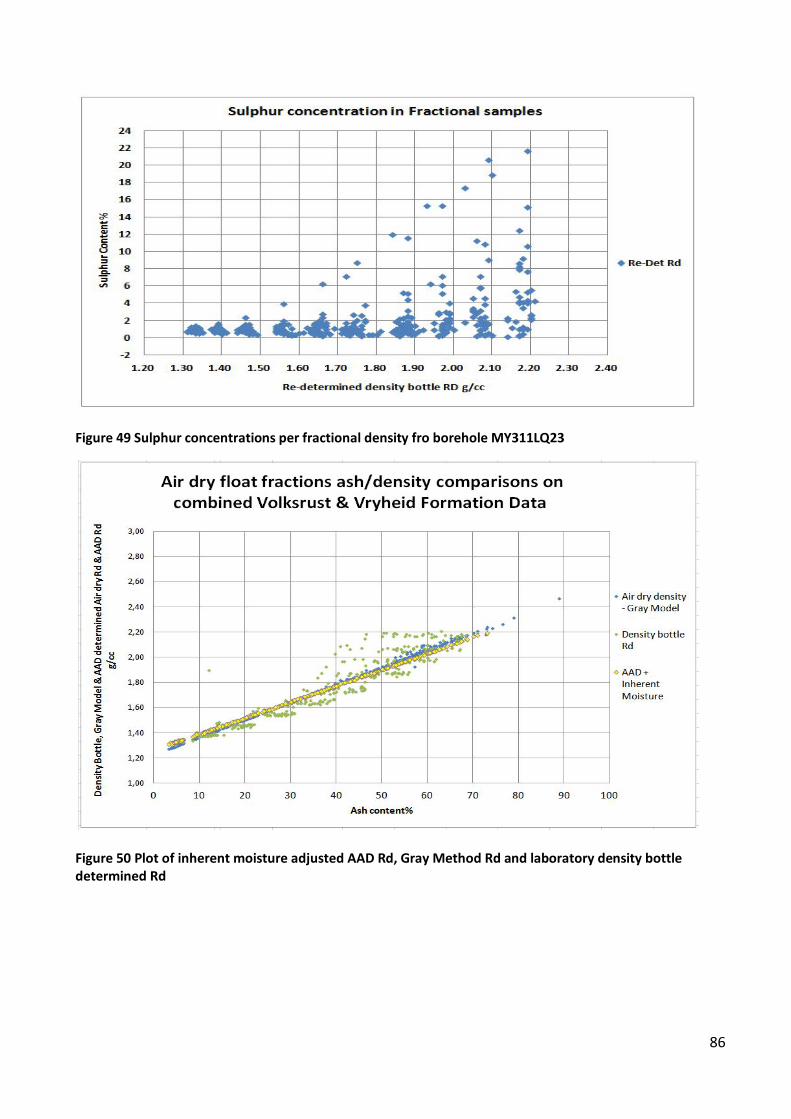
86

Figure 49 Sulphur concentrations per fractional density fro borehole MY311LQ23

Figure 50 Plot of inherent moisture adjusted AAD Rd, Gray Method Rd and laboratory density bottle determined Rd

87

Figure 51 Plot of absolute dry density obtained from AAD against the Gray model and density bottle determined densities.

Figure 52 Descriptive statistics for the differences between Gray method and AAD moist adjusted as well as between Gray method and AAD

88

The calculations done did not include estimations of in situ moisture and the final estimation for an in situ relative density. Not having any data relevant to moisture content of the cores on recovery led to the determinations being terminated at an air dry equivalent. A further set of samples were taken randomly from a borehole in the deeper part of the Waterberg coalfield where the entire succession was well below the regional ground water table. The purpose was to test specifically for various density determinations as well as helium pycnometry, in an attempt to justify the decision to terminate evaluations at an air dry equivalent value. The results are portrayed in Table 12. The samples had initially not been impeccably preserved, thus the field mass was partially dry. Samples were then sent to an external laboratory for specified relative density determinations that they were unable to do, they were then stored for approximately 7 months before being sent to another laboratory for helium pycnometry. The first set of data was derived on an as received basis. The samples were then dried at 105 deg centigrade for 24 hours and retested giving more representative air results. The final set of data was determined after the samples had been re-submerged in water for 48hrs, again giving a different set of results. This illustrates the susceptibility of the samples to moisture absorption and raises doubt with respect to densities other than air dried densities for reserve calculations. The variability of results obtained is directly related to the effective porosity of the samples and surrounding environmental conditions.

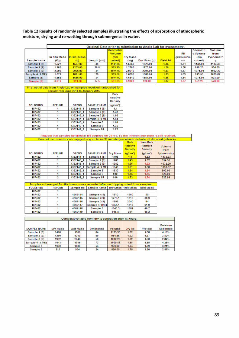
89

Table 12 Results of randomly selected samples illustrating the effects of absorption of atmospheric moisture, drying and re-wetting through submergence in water.

90

6.1.4 Evaluation Of Field And Laboratory Sample Data The information in the following tables represents a series of results from a full succession borehole intersecting both Volksrust and Vryheid Formations, the purpose being to portray the basic information derived from exploration core samples, initial mass and SG determinations and core recovery determinations. This absolute basic data forms the basis from which all other resource relevant determinations are made. The samples are in chronological order from sample 1A at the top of the stratigraphic section through to sample 32 at the base of the succession. All the identified coal zones from the upper coal zone 11 to coal zone 1 at the base of the succession are represented. Although The Law of Superposition indicates that the oldest rocks in a succession are at the bottom. The sample numbering sequence in the Waterberg coalfield conforms to the order that the pioneers in this coalfield used for sample labelling, it has been accepted and used for correlation purposes historically by everyone that has done any exploration work in the Waterberg coalfield. Data from the original core recovery sheets, as compiled at the mine for the individual coal and shale samples, was used as the basis of this compilation. These individual sheets containing basic data for the separate coal and shale components of the sample were combined using the product of the coal samples mass and length added to the product of the shale samples mass and length and the divided by the total length of the sample to obtain a weighted mass for the combined sample (I.e. this is a composite of the coal and shale encountered in the sample interval.). Table 13 presents the shale component, its mass in air, its mass in water, its Archimedes determined SG which was done in the field due to the broken nature of the core after sampling and separation of the coal and shale components, the sample thickness, its calculated mass based on the Archimedes determined SG and the volume represented by the area of the core and the total thickness of the shale separated from the coal stringers in this sample. Its calculated recovery percentage based on the difference between its calculated mass and its measured mass in air was then determined and reported. Note, this procedure was enforced and stipulated as standard practice by the geology principals in the company. (the interpretation of this so called recovery assumes moisture saturated core, which would result in the SG being representative of the solid portion disregarding the moisture in the pores, if the sample had been submerged long enough for the displacement of all air thus it is not representative of the relative density of the whole sample.) Table 14 and Table 15 respectively present the same data for the coal component and the composited combined coal and shale representative of each individual sample.

91

Table 13 Basic datasheet for shale samples prior to dispatch to laboratory for analysis.

It should be noted that these sheets have been compiled on historical formats and that certain assumptions are associated with the data presented. Drilling of a 120m+, large diameter cored borehole could take between 2 to 3 weeks to complete, allowing another week for depth corrections and the marking of the core with respect to lithologies and depths prior to geological logging and the compilation of a geological profile for correlation and sample delineation prior to sampling the core would have been exposed to atmospheric conditions for a minimum period of a month before actual sampling was done. No effort at preserving the in situ moisture of the core on recovery was made. The core was then sampled and the samples split into coal and shale components, thereafter it was then transferred to a core shed where initial weight in air for the individual samples was measured. Thereafter the samples were subjected to the determination of their weight in water as prescribed for the Archimedes SG determination. This value was then used to determine the purported true mass of the sample and relate this to core recovery.

92

Table 14 Basic datasheet for coal samples prior to dispatch to the laboratory for analysis.

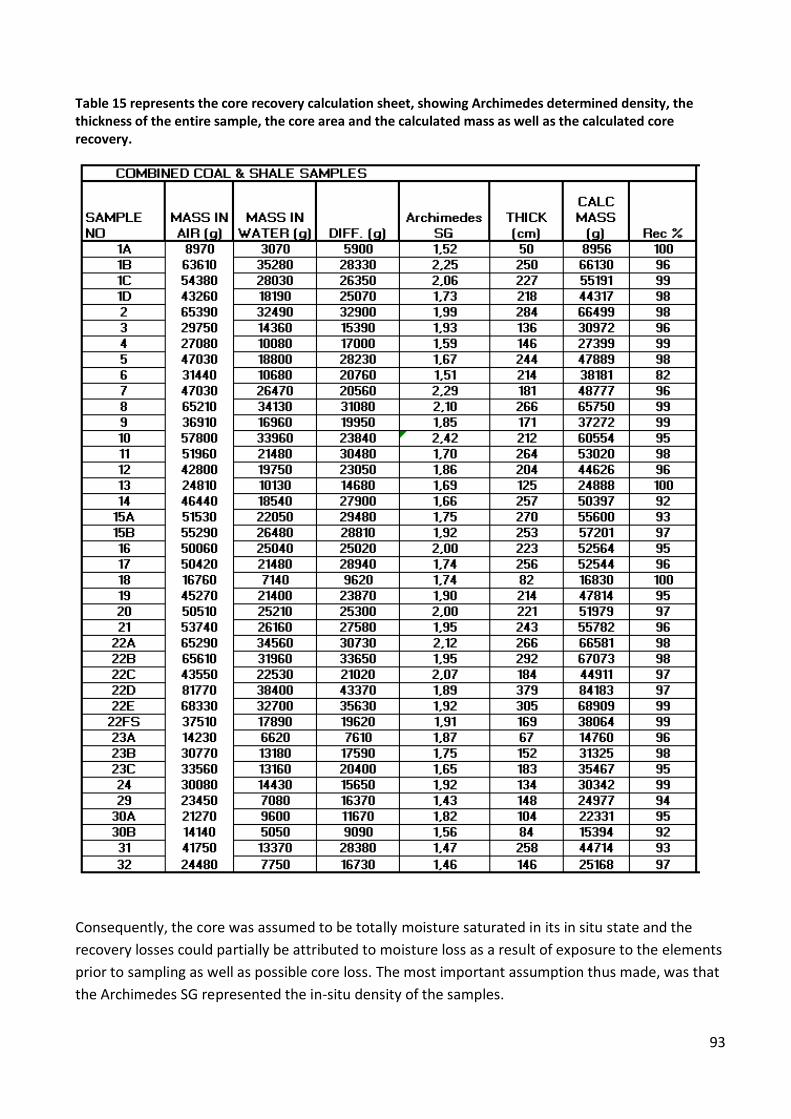
93

Table 15 represents the core recovery calculation sheet, showing Archimedes determined density, the thickness of the entire sample, the core area and the calculated mass as well as the calculated core recovery.

Consequently, the core was assumed to be totally moisture saturated in its in situ state and the recovery losses could partially be attributed to moisture loss as a result of exposure to the elements prior to sampling as well as possible core loss. The most important assumption thus made, was that the Archimedes SG represented the in-situ density of the samples.

94

Table 16 has two additional columns representing the samples calculated geometrical volume and a field mass determined relative density based on the mass in air divided by the geometrical volume of the sample.

Table 16 additional calculated values based on the basic core recovery sheet data.

From the data presented above it will be noted that the density values obtained from the hydrostatic determination (Archimedes) conducted on all the samples, as opposed to the calculated densities derived from the field mass of the sample divided by its geometric volume indicate a

95

discrepancy with regard to moisture content between the two sample sets. Although the trends appear relatively close when the two sets of values are displayed graphically as illustrated in Figure 53, the actual values are not close. These values have been plotted sequentially to illustrate the differences between each sample. These differences could be indicative of porosity/moisture content variations due to their composition and the coal/shale ratio in the Volksrust Formation. The samples in this vertical intersection of the coal succession were also below the regional groundwater table at the time of drilling this borehole, and as such, they could have been moisture saturated. The free moisture content retained in the cored samples at the time of sampling may have been relatively high.

Figure 53 A sequential plot of Archimedes-determined in situ density opposed to field mass core mass/volume derived density for each sample in the Waterberg coalfield succession.

On the basis of these results, neither of the two density values, i.e. not the Archimedes Relative density (Rd) or the Field mass determined Rd, are suitable for resource estimation. The major deficiency being that no data pertinent to the original moisture content of impeccably preserved core on recovery was available. The next set of data that was evaluated was the laboratory information. This data supplied information from receipt of the samples, through initial sample preparation, crushing and screening to -13mm +0.5mm and air drying under controlled temperature and humidity, followed by float/ sink washability tests and proximate analysis of each fraction. The evaluations of proximate data through the application of the AAD methodology, to obtain the true dry density of the matrix material in the samples, were then undertaken. The proximate data from which the ash percentage

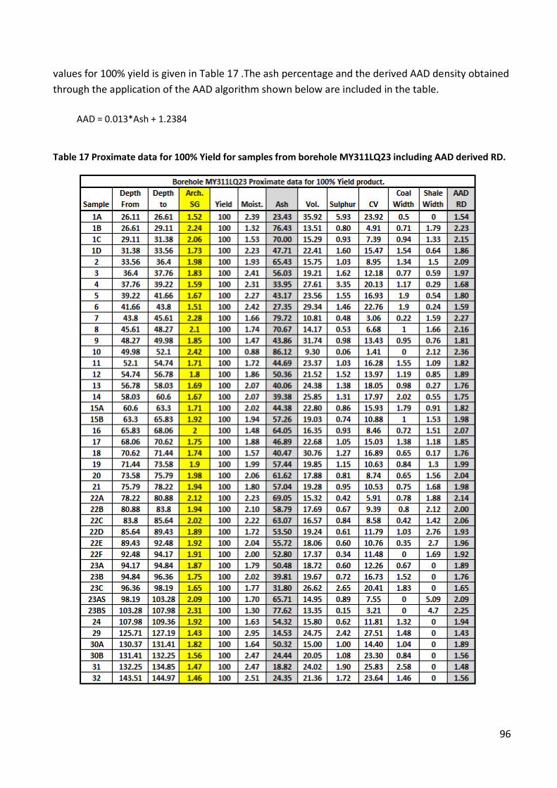
96

values for 100% yield is given in Table 17 .The ash percentage and the derived AAD density obtained through the application of the AAD algorithm shown below are included in the table.

AAD = 0.013*Ash + 1.2384

Table 17 Proximate data for 100% Yield for samples from borehole MY311LQ23 including AAD derived RD.

97

Detailed information regarding the samples from this borehole is summarized in Table 18. This includes the basic field masses and field-determined Archimedes Rd, laboratory masses for both the initial received mass of the samples and the crushed air dried mass, the inherent moisture percentages and the pycnometer-derived density as well as all the calculated densities that could be derived from these data. The crushed -13mm and +0.5mm screened and air dried sample mass including the mass of the -0.5mm fraction relative to the original volume of the sample provided a density value that could be considered acceptable as an air dry Rd because the sample had been dried in the laboratory under controlled conditions relevant to temperature and humidity. Table 18 Summary of field, laboratory and calculated data.

98

In addition, density determinations via pycnometry as prescribed by AS1038.21 part 4, was requested for each float fraction of all the samples submitted. These results were composited for each sample to determine the sample’s apparent true density. The process for compositing the samples involved firstly cumulating the fractional data for the separate coal and shale portions of the samples to obtain an apparent relative density for the coal and the shale and then combining the coal and shale portions by mass weighting to determine the sample’s apparent true density. The summarized results obtained for each sample and the different methods of determination are portrayed in Figure 54, Figure 55 and Figure 56. The sequential plot in Figure 54 illustrates the differences between Archimedes determined Rd, Pycnometer determined total apparent true density and the inherent moisture corrected Rd derived from the application of ash adjusted density (AAD) algorithm as portrayed in Table 17. The pycnometer densities appear higher than the AAD densities; this may be due to additional absorption of moisture from the wetting agent when undertaking the determination. Although a great portion of the macro and cleat porosity may have been destroyed during grinding to -212 micron, it is believed that micro porosity capable of absorbing moisture still existed in the pulverized particles resulting in a misrepresentation of the true density of the dry matrix material. The AAD Rd on the other hand takes the total destruction of the combustible component into account to give a true dry Rd value for the sample; this is then enhanced by adding the inherent moisture component so that comparisons can be done on the same basis. The Archimedes determined density merely gives an indication of some water absorption increasing the overall density of the sample. The results displayed below also show that the samples were not submerged long enough to satisfy the expulsion of all the air or gas from the interconnected pores. If this had been the case, the Archimedes results should have complemented the pycnometer results.

Figure 54 A sequential plot of density values obtained from the Archimedes principle, Pycnometer (AS1038.21 part 4 and the inherent moisture corrected AAD calculation for the total apparent density value’s of the individual samples.

99

The sequential plot in Figure 55 shows an exceptional correlation between the -13mm +0.5mm air dry crushed material densities obtained in Table 18 and the densities derived from the field samples, where the densities have been derived from the basic field mass(mass in air of recovered core) using the density equation, (I.e. Rd = mass/Volume, mass being determined in air and volume of the core determined from its area and length). The correlation between these two sets of values is 99.98%, suggesting too that the field mass could be used to represent an air dry density. Climatic conditions and time of exposure to the elements prior to sampling was sufficient to dry the core effectively. This however is not always applicable.

Figure 55 A sequential plot of the -13mm +0.5mm air dry determined density against the field determined density. Note that the values plotted correlate perfectly therefore the plots overlap.

The sequential plot in Figure 56 highlights the difference between the true relative density values (i.e. the moisture adjusted AAD plot) and the apparent air dry density (the red squares). The difference between the plots illustrates the effect that possible moisture holding capacity or effective porosity can have, i.e. the air dry plot reflecting lower relative densities as a result of effective porosity.

100

Figure 56 A sequential plot of the moisture corrected AAD density for the absolute density of the solid matrix and the air dried density determined from the -13mm + 0.5mm material.

Table 19 Correlations between determination methods.

Based upon the results above, it was proposed that the raw ash AAD value be used instead of the Archimedes Rd but, on testing, the results only gave a 97.24% correlation. The sequential plot in Figure 57 summarizes the findings of this evaluation, showing the overall composition of the samples relative to the main components, I.e. Coal, Mineral Matter, Inherent moisture, probable porosity or moisture holding capacity. The best density derivates are also plotted to illustrate possible losses or effective porosity between the true relative density (inherent moisture corrected) and the -13mm+0.5mm air dry density. From this figure it will be noted that air dry RD and AAD moisture corrected RD clearly follow the same trends (higher Rd in both plots equals higher mineral matter content). But it is also apparent that the AAD Rd values are higher than the air dried values in most samples, coming closer to one another when the mineral contents are highest.

101

Figure 57 sequential plots of the individual sample’s composition with regard to coal, indestructible mineral matter (represented by residual ash), porosity and inherent moisture within the Waterberg Coalfield succession as well as the selected densities for total true density and air dry density.

Figures 56, 57 and 58 illustrate the comparative values when calculating the forms of mineral content or ash in the coal samples under review. Here it will be noted that the Parr method provides a higher value than the proximate ash analysis supporting the theory that some mineral volatile content is lost during combustion. It should however be noted that the mentioned losses are a combination of volatile mineral matter and moisture. Figure 59, a plot showing the same data as Figure 56 and including a bar representing the Ash content plus inherent moisture shows that very little mineral content is lost in respect to the purer coal samples, as the shale content increase the difference becomes greater. The losses however appear to be relatively consistent. Figure 60 depicting a comparison between geological core logging and visual descriptions of the core shows a poor correlation between the visually determined coal to shale ratio in comparison to the Parr determined mineral content values. It is therefore concluded that the Parr method’s determination of mineral content Vs Inherent moisture corrected Ash content method of calculating mineral/matter of ash content, is better and more accurate than the latter moisture corrected ash content method when assessing the relative density of a coal.

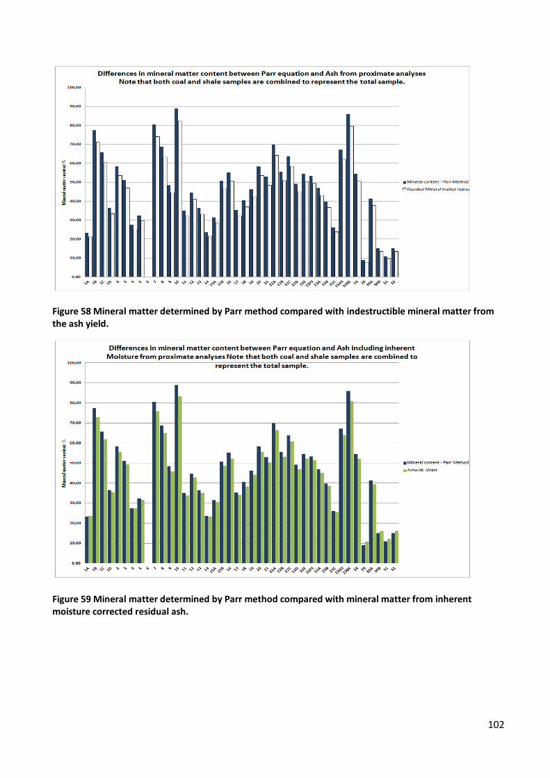
102

Figure 58 Mineral matter determined by Parr method compared with indestructible mineral matter from the ash yield.

Figure 59 Mineral matter determined by Parr method compared with mineral matter from inherent moisture corrected residual ash.

103

Figure 60 Comparison of mineral matter determined from Parr method and geological lithology

A proper understanding of the composition and primarily the relationship between coal density, coal porosity and moisture content as well as accurately measured moisture content from impeccably preserved samples are of paramount importance in determining the correct values with respect to the in situ density of raw coal. It is therefore apparent from all the results obtained to date that the ash adjusted density provides the best approximation of the dry density of the matrix material. This value is then corrected to represent the air dry density of the solid matrix by including the effect of the inherent moisture content determined from proximate analysis to the AAD value. In the absence of an accurately determined moisture holding capacity value, the crushed, -13mm +0.5mm screened mass representing the air dry mass for the sample can be converted using this mass divided by the originally determined geometric volume of the core sample to ascertain the sample apparent air dry density. The difference between this density value and the inherent moisture corrected AAD value would then be representative of the voids in the sample, in other words, would be its effective porosity. This exercise however does not allow the determination of the possible in situ Rd of the samples, since no values representative of the moisture content of an impeccably preserved core retrieved from the exploration site or the effective porosity of the samples were available.

104

7. RECONCILIATION OF RESOURCES AND RESERVES

This Chapter will present an over view of the application of the density methods in coal resource and reserve assessments with a view to calculating reconciliation values for a mine.

7.1 INTRODUCTION Reconciliation is essentially the process of identifying, analyzing and managing variance between stated origins, predetermined values and actual results so that differences can be recognized, highlighted and explained. These differences encourage the creation of methods improving estimates, designs, tighter and more accurate plans and schedules, improved mining techniques minimizing ore loss and dilution and identifying ways of increasing product recoveries during the extraction processes. The ability to measure and analyze data in this way enables an operation to design and implement process improvements across the entire value chain. (Riske, 2007) A range of activities common to most deposits is recognized across the value chain. These activities include resource estimation, mine design, planning, grade control, mining, material transfer, and ultimately mineral processing. An inverted pyramid, Figure 61 serves to illustrate the flow of information. This can be used as a starting point with an increase in available information as the pyramid grows to the subsequent layers representing processes in the value chain above. Each subsequent process is represented by a layer in the upward expansion of the pyramid and is dependent on information from the previous layer. Reconciliation of data in these respective layers serves as a reality check between these layers enabling transparency of data and information. Reconciliation can then be broadly categorized into three main areas, namely, spatial, temporal and physical using this technique.

The most important aspect of any reconciliation process is to ensure that an estimate against a measurement must be for the material, for which the estimate has been made against the same material being measured.

The preliminary reconciliation of cardinal importance relates to the spatial reconciliation scenario which is the three dimensional or X Y and Z, form of reconciliation and is derived from comparison of predictive models or actual measurements based on a geographic location.

105

Figure 61 represents the inverted reconciliation pyramid – temporal, spatial and physical reconciliation.(Riske, 2009)

Spatial reconciliation measures the absolute performance between predictive models and actual results determined by mapping, survey measurement and analytical data coupled to the spatial point’s extraction results.

The data used in these predictive models forms the foundation for all the processes in the value chain that follow.

The value of the reconciliation data remains dependent on the quality and reliability of the input data, namely the estimates and the measurements.

The most basic properties with reference to the resource such as the in-situ density of the commodity have to be accurate so that the gross in situ resource tonnages, from which the mineable reserves together with the saleable products are determined for the deposit, are credible.

The evaluation of the original data from the exploration boreholes, samples taken and analytical data representative of the samples taken is crucially important when utilized in the construction of predictive models since qualities and product yields are estimated from these models.

This spatially oriented information forms predictive data between points of actual data that must be comparable with the original geological interpretations and analytical data obtained from the samples and the subsequent composition of mining units associated with the distribution of the known data points.

The values pertinent to the material used for analytical data also have to be corrected to comply with the original mass (i.e. if a representative portion is removed from the original sample, physical properties of this portion after sample preparation in relation to the original need to be known, and the analytical data obtained is to be adjusted accordingly when reference is made to the origin).

Since the commodity is coal, an accurate determination of the in situ density is required for gross in situ resource tonnage determination. Selections of approximately 48-61 large diameter cored boreholes were chosen in the investigation area for the resource evaluation. The large diameter boreholes are more representative of exploration work done since the mid to late 1980’s and provide more raw materials for most of the analyses required. The large diameter cores have also been found in general to give better results due to improved recoveries.

7.2 RECONCILIATION OF PRELIMINARY FIELD & LABORATORY DATA This flow chart shown previously has been repeated for references to the processes and data available from the exploration borehole to the laboratory is included to illustrate the recorded data that could be evaluated for reconciliation purposes.

106

Figure 62 Flowchart of processes and data available from an exploration borehole through the laboratory and back to the original site.

An assessment of the flowchart reveals four sets of data with respect to masses that can be compared to give some indication of possible moisture contents and losses from the original sampled drill core to the crushed and screened product before float sink analysis. Note too that the material outside the prescribed range for crushing and screening is included in all situations. The material referred to pertains to the -0.5 mm fraction, this fraction is also weighed and although it represents less than 0.8% average of the samples is included in density determinations of the air dried -13mm, +0.5mm portion, and it also represents the raw proximate analytical values. Data relevant to field mass, laboratory received mass, crushed and screened masses as well as the -0.5mm fraction, Archimedes SG, ash yields, moisture content and calorific values was extracted from the geological and analytical database for the mentioned boreholes and evaluated in excel spreadsheets. The most important aspects of this evaluation are summarized in Table 20, here densities for each respective method for each of the mining benches have been used to ascertain the best combination in order to provide a credible relative density to use for tonnage estimation. It is impossible to derive a credible density value for the in situ material without information relating to the free moisture content and effective porosity of the samples that should have been determined from impeccably preserved core. It is therefore suggested that the resource and reserve tonnage estimates be based on the -13mm +0.5mm and -0.5mm air dry relative density values that have been re-constituted to the original volume of the sample. These relative density values are more conservative and probably closer to the apparent relative density of the material being evaluated in this open-cast mining operation. Should the Archimedes density however be used to determine gross in situ tonnages then the equivalent loss factor between the -13mm +0.5mm relative density and the Archimedes density could be used as a geological loss factor. This however may not give an accurate result, unless the

107

core when submerged in water for its mass determination in water, was submerged long enough for the water to displace all the air/ gas within the interconnected porosity in the core to satisfy complete saturation status. In Table 20 below the relative densities obtained via the different methods for the respective mining benches are summarized. The density values were obtained from composites of the sample assemblages representing each mining bench, an average thickness for the benches is shown as well.

The Archimedes (Average Raw Rd) was obtained through a weighted composition of Archimedes densities for the individual samples constituting the mining bench.

The average Field mass density was derived from the basic equation where the sum of the recovered field masses per sample in the bench configuration is divided by the total volume of the samples in the same configuration.

The laboratory RD was obtained from laboratory received masses for the respective samples per bench configuration.

Lastly the Air dry -13mm,+0.5mm and -0.5mm RD was obtained from the mass of these air dried samples divided by the total representative volume of the core representing the bench configuration.

The losses expressed as percentages were obtained by accepting the -13mm,+0.5mm and-0.5mm air dry RD as being representative of the solid matrix. This was then expressed as a percentage of the total derived by the Archimedes RD and the difference between the 100% value obtained from the Archimedes RD was expressed as a loss. The same process was applied to the differences between the air dry Rd and the other densities obtained. Assessing the tabulated values it then appears that there is a moisture loss between the field mass and the laboratory received sample as well as between the air dry value and the original determined Archimedes RD Table 20 Summary of relative density values obtained via the different methods and possible associated losses based on the basic information on hand.

108

Taking the evaluation a step further in Table 21 by introducing the ash adjusted density values which reflect the true dry density of the solid matrix and correcting these with the inherent moisture determined from the proximate analysis (an average of 2%) serves to produce a value which may represent the true air dry relative density, once again of the solid matrix. The density value determined from the mass of the -13mm +0.5mm air dry sample expressed as a percentage of the aforementioned inherent moisture corrected AAD Rd would then give a reasonable approximation of the true effective porosity or moisture holding capacity of the sample. The -13mm + 0.5mm air dry Rd however appears to be the most accurate representation of relative density for the sample and should be used for reserve and run of mine tonnage estimations. Table 21 Summary of relative density values extended to include values determined via the ash adjusted density algorithm and the inherent moisture corrected AAD relative density.

Using the Archimedes Rd shown in Table 22 to predict gross in situ tons results in a tonnage of 1,554,301,392 tons in a reserve area of 1091.24Ha. The tonnage derived from the -13mm + 0.5mm air dry Rd is 1,385,579,144 tons, which is 168,722,248 tons less. This is an overestimation of 10.86%. The AAD moisture corrected Rd should be used since this value represents the true air dry density of the matrix. The results of this application are shown in Table 23 the averaged amount totalled translates into a loss of 14.06% in this reserve block for a combination of all the mining horizons.

109

Table 22 Summary of mining bench information showing predicted tonnages using the Archimedes determined Rd and expected tonnages from the -13mm +0.5mm air dry Rd as well as the differences and percentage overestimation on an area of 1091.24 Ha.

Relative density determinations based on the initial datasets were calculated and compared in order to establish the most appropriate for an in situ relative density determination. The comparisons between the Archimedes determined relative density and both the densities determined using the field mass and core volume as well as the laboratory mass and original core volume revealed possible moisture content ranging from 2% to approximately 8.5% if the entire succession was taken into consideration. The lowest values ranging from 2% to approximately 5% were obtained from the samples in Coal Zone 3 and Coal Zone 2, i.e. in the Vryheid Formation which is inertinite rich, and with coal seams exhibiting higher macro porosity thus aiding faster drainage of moisture from the matrix structure. The Volksrust Formation, which is vitrinite rich and therefore exhibiting greater micro porosity, appears to have retained more moisture ranging from 4% to approximately 8.5%. Table 23 Summary of mining bench information showing predicted tonnages using the inherent moisture corrected AAD Rd representative of the air dry solid matrix and expected tonnages from the -13mm + 0.5mm air dry Rd as well as the differences and percentage overestimation on an area of 1091.24 Ha.

110

7.2.1 Discussion - Introducing the relative density determined from the -13mm+0.5mm and the -0.05mm air dried, crushed and screened sample representative of the original core volume, highlights the difference between this density and the Archimedes determined value which increases the loss percentage to values between 9% and 14.6%. Note that these values are only indicative of the amount of moisture absorbed by the core sample during the Archimedes determination and that they do not give any indication of the effective porosity in the solid matrix of the core sample. These results are merely representative of absorbed and adsorbed moisture attained during the duration of the core being submerged in water for the Archimedes determination. If individual bench composites were examined, the porosity percentage could be more accurately ascertained if an inherent moisture correction on the ash adjusted density were used. Applying the foregoing to the data on hand then raises the differences in tonnages into a range from 9.4% to 17.3%. The values obtained representing the Volksrust Formation would therefore range from 12% to 17.3% and the Vryheid Formation from 9.4% to 11.4%. This evaluation results in the following observations:

Borehole core samples were not impeccably preserved for a laboratory moisture content determination.

Neither the Archimedes nor the field/laboratory determined relative densities are suitable for an in situ relative density determination because no acceptable accurate information with regard to the free moisture content or the effective porosity in the core is available.

The only remaining alternative would be to use the -13mm+0.5mm air dry determined relative density to provide a reserve value for the solid matrix.

Introducing the ash adjusted density derived from proximate analysis and correcting this to accommodate the inherent moisture determined from analyses at least gives an accurate relative density for the solid matrix. The difference between this value and the -13mm+0.5mm air dry determined relative density would then be indicative of the void percentage within the sampled sequence representing the bench composition.

This value could then be used as a correlation factor to adjust the inherent moisture corrected AAD relative density, for tonnage reserve calculations. Tonnages thus determined would also be reflective of expected run of mine tonnages.

The loss values determined for the Volksrust Formation are in the range 12% to 17.3%, and for the Vryheid Formation 9.4% to11.4%.

Gross in situ values cannot be determined without data providing accurate estimations of free moisture and probable effective porosity.

111

7.3 RECONCILIATION FROM A MINING UNIT PERSPECTIVE

7.3.1 RESERVE AND DESIGN BACKGROUND Reconciliation of field and laboratory data gives a very broad indication of the importance and relevance of the basic geological information and the critical role it portrays in the structure of the value chain on which the entire process in evaluating the resource is based. If this basic initial information is suspect the rest of the value chain is in jeopardy. The main points to consider are first, a basic structural model defining the geology within the explored resource. This requires data concerning the encountered lithologies, coal seams, probable structure and initial proportions relating to probable resource amounts relevant to volumes have been established from the exploration drill core interpretation along with seam correlation and sample delineation. This basic work allows the delineation and definition of the mining horizons for commercial extraction. Mining values relevant to seam roof, seam floor, coal qualities and associated properties and a host of other applicable values can now be incorporated into this model. The actual resource and mineable reserve tonnages can be determined using the density data for the relevant horizons and the predetermined defined volumes for those delineated horizons. This basic model is used by mining engineers to design the mine layout and to select the mining methods to be applied along with the coupling equipment to these methods, and also to design the mining units with their relevant characteristics on which the basic metrics are based. The design phase refers to the operational method formulated on the economics of extraction, namely, the following:

volumes, hauling distances between the deposit and the beneficiation plants, life of mine based on material availability, structural constraints, Stripping ratios etc.

In a very broad sense the metrics associated with the mining aspects all have relevance to the geological model and its economical viability. Once the mining engineering aspects have been designed, , the layout is returned to the Geology department so that the mine design can be populated with the required relevant quantity and quality information pertinent to the deposit within the defined limits designed by mining engineering. The values assigned to the various mining horizons and units are required to be adjusted to take geological losses, modeling losses and mining losses into account. Overall these losses result in a reduction of the resource’s determined tons, based on tonnages derived from the in situ relative density of the raw material relative to each relevant phase. This however, is not the case because:

112

The original estimate was not based on the in-situ relative density of the resource. The in-situ relative density of the resource could not be determined since the core was not

impeccably preserved on recovery and no attempt was made to determine the moisture content of the core at recovery.

The Archimedes SG was determined only after the core had been logged geologically, correlated and sampled according to the sample delineations defined, this process was conducted, at best, four to six weeks after the borehole had been completed.

The Archimedes determined SG was used as a basis for tonnage determinations relevant to gross in-situ tonnages as well as by all departments involved later in the value chain with regard to predicted tonnages, planned tonnages, survey predicted tonnages for mining blocks staked and reconciliation evaluations after mining.

Possible geological losses pertinent to the material being mined to determine a suitable correction factor to apply to tonnages derived was not ascertained, thus an arbitrary factor related to structure and possible unconformities was used to reduce tonnages from gross tons in-situ to reserve tons. The geological loss correction factor, however incorrect the value may have been was only applied to tonnage estimations but not to the basic information such as the relative density values for the respective, samples, zones and mining benches for reserve calculations prior to determination of mineable reserves, to ensure continuity for comparative purposes.

The only solution thus was that a credible estimation for probable run of mine tons recoverable from such a reserve needed to be formulated. Currently the data that is estimated is then forwarded to planning and scheduling departments to formulate the process flow from the mine to the various beneficiation units. The information used in this evaluation refers to set polygons representing individual numbered mining units obtained from the mining engineering layout on each vertical mining horizon throughout the stratigraphic sequence.

7.3.2 PLANNING AND SCHEDULING (Information only) The schematic in Figure 63 Illustrates a sectional projection through the probable mine layout, with mining horizons identified and further subdivided into mining units of defined geometric specifications. Quality and expected tonnages have been allocated to these units from information extracted from the geological model for planning and scheduling purposes. This data is used by the design and planning engineers for the scheduling of the mining units to be extracted for beneficiation, based on their required properties and yields of specified products. Figure 64 is an example of the scheduling, showing the mining units, color coded for the period in which they are planned and scheduled to be mined. Note that the information supplied to the mine planning department for the scheduling of mining units needs to include the initial losses from the resource and reserve estimations through to estimated run of mine tonnages.

113

Figure 63 Schematic layout of proposed mine plan.

It is vitally important that this data is as accurate as can be estimated since the operational phase which is based on client product and tonnage requirements or demand, uses this data for an annual production budget. The most important factor to bear in mind when these estimations are calculated is the fact that the entire operation’s infrastructural setup and logistical support rests on the basic information relevant to the quantity and quality of the ore body being exploited. Requirements with respect to equipment, personnel, beneficiation facilities availability and capabilities are all inter-related to the material available for exploitation.

Figure 64 Schematic of scheduled mining units on different benches/mining horizons.

114

Returning to the basic mine plan, the coal deposit has been evaluated, layout and mining horizons defined and an extraction strategy for the mine formulated. The mine plan is then overlain over the coal deposit and the mining horizons are subdivided into strips, with the strips being further subdivided into mining units or blocks. These blocks are then scheduled for extraction to one or more of the various beneficiation plants for the production of a range of products at specified qualities. The qualities of the products range from ash content and calorific value but also include a host of additional specifications relevant to sulphur and phosphorous content as well as product sizing constraints. The planning department has to assess all the relevant information relating to the operation such as equipment required, mining tempo’s required to meet demand and the amount and quality of raw material being exploited to meet demand. If the basic information, especially relevant to the expected tonnages of raw material, is not within an acceptable confidence level, expected production will not be achieved. Requirements with regard to expected tonnages may then need to be met through increased throughput, thereby introducing additional costs and constraints. The significance of correct estimations is not relevant to a monetary amount but to the depletion of the resource as a result of increased extraction volumes required to meet targets. Consider a 15% over estimation of resource tonnages on a 40 year life of mine (LOM) as an example. This would mean that the original estimated resource would be depleted in 34 years, reducing the proposed life of mine by 6 years. The planning and scheduling phase is considered as the basis for the operational phase on which the metrics to be used for reconciliation, grade control and model refinement are based. Examples of these metrics have already been used in this thesis to determine and validate relative densities, as applied in the resource and reserve estimations. The geological model for this overall plan is based on a measured grid of exploration boreholes with the smallest spacing being 250m apart and up to 500m and 1000m in some cases. Once the mining horizons have been defined, the physical properties and analytical qualities are spatially modeled for each of these mining horizons. Allocations for the polygons representing the mining units, normally 250m long by 50m wide, are extracted from this model and used for scheduling purposes. These values per se, would be representative of the ideal situation relating to the various polygons’ geometric parameters, properties and grade qualities. The properties include raw relative density, yields of specific products and expected qualities related to these products. Each mining unit has specific properties associated with that specific horizon as extracted from the spatial geological model for that horizon. The grade control section now applies the information to make the necessary adjustments when taking actual production from each mining horizon into account. For the purpose of this thesis and to prove the points presented by way of example, two mining horizons, one from the Volksrust Formation, horizon 3 and one from the Vryheid formation, horizon 6 have been selected for this reconciliation evaluation. The geological model information obtained from the 2010 geological

115

model built in MINEX (Geological Modeling software supplied by GEMECS) was utilized for planning and scheduling in Mine Works Planner.

7.3.3 VOLKSRUST FORMATION MINING UNIT DATA

In Figure 65 below, mining units in three mining strips on mining horizon 3 were selected to give a reasonable overview of an area in the open pit. They are mining strips, B03/92, B03/93 and B03/94. Table 22 portrays the values of the planned blocks as set out in the mine schedule and populated with data from the geological model. Two columns in this table have been highlighted to illustrate small differences between values extracted as (i) a polygon representative value from the model and (ii) the same value calculated from given parameters relevant to the area. The average thickness of the seam representing the mining horizon is provided. Table 24 indicates the total modeled run of mine tonnage for this exercise is given as 6,476,900 tons, while the planned and survey demarcated and staked area for drilling, blasting and loading run of mine tons were 6,703,137 tons. The last three columns represent differences influencing the variance in tonnages between the two sets of values. These blocks were then blasted, mined and material tonnages recorded as dispatched to the various beneficiation facilities. This data as shown in

Table 25 formed the initial as mined data for these mining units. Each mining unit was surveyed on completion to determine the volumes of material that had been extracted and an adjusted survey tonnage relating to the volume was determined. Floor elevations were also measured to ensure that the mining unit conformed to its specifications. This gave a

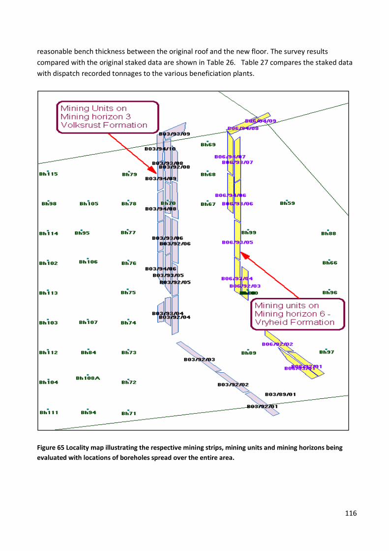
116

reasonable bench thickness between the original roof and the new floor. The survey results compared with the original staked data are shown in Table 26. Table 27 compares the staked data with dispatch recorded tonnages to the various beneficiation plants.

Figure 65 Locality map illustrating the respective mining strips, mining units and mining horizons being evaluated with locations of boreholes spread over the entire area.

117

Table 24 Comparison of model extracted information relating to the area of the mining units, the model thickness of the bench and the expected tonnages based on the Archimedes Rd, geological loss factor adjusted compared with surveyor’s staked information when these units were marked out for drilling and blasting. The survey Rd’s used for tonnage determinations were the raw Archimedes Rd allocated to that specific block.

Table 25 Comparison between staked values and the actual mined values reported for the duration of the loading and hauling period that these units were extracted, the last three columns again displaying differences in the main parameters.

118

Table 26 Comparison between the planned survey staked data(pre drilling, blasting and loading), and the final mined, surveyed data also highlighting the differences in the main parameters between the two datasets.

Tables 24, 25 and 26 highlight differences between the geological model area, volumes and tonnages and those of the survey staked values prior to mining, the as mined reported values and

119

the final survey information relating to the mined out area, which all have an effect on the end product, tonnages. In respect of the model values against the survey staked and as mined values, discrepancies with regard to tonnages can all be attributed to the geometry of the blocks planned, their areas, seam thicknesses and derived volumes, since the same density values for each block were used. These tonnages were obtained from the raw density determined via Archimedes principle. The final surveyed area, surveyed areas and volumes were used to determine the seam thicknesses and the surveyed tons and volume were used to determine the relative densities for each block mined. A further reconciliation regarding the dispatch reported tonnages still had to be considered. A comparison between the survey staked tonnages and the dispatch reported tonnages was done and the findings shown in Table 27. In Table 27 the column referring to Total dispatch tons represents the tonnages reported by the dispatch system and the mine lookout post. A survey bulking factor was applied to derive corrected tonnages for the volumes mined. This bulking factor was a factor calculated by the survey department based on averaged volumes of material loaded into the specific size tip of the various haul trucks and the averaged tonnage represented by these volumes. Tons in this case were determined over a weigh bridge to improve accuracy. These factors were used by survey to adjust loads hauled by these trucks. The values should represent the tonnages from the appropriate staked blocks, however inaccurate GPS data linked to the dispatch system, poor supervision and reporting from the in pit operation led to inaccurate block reporting within the mining area. The inaccuracies were invariably associated with block boundaries especially in situations where portions of scheduled blocks were drilled and blasted out of sequence or due to emergency requirements. A larger area incorporating several blocks was chosen so that a more representative sample of a period of mining could be evaluated. The planned and staked blocks values could then be adjusted to the same representative area and volumes that had been measured by survey to derive the expected model and staked tonnages for the same area using the model density values allotted to the blocks in the same mined area. Tables 28 to 30 present additional comparisons namely, Table 28 is a summary of the various tonnages from predictions, as well as measured values from a survey vantage and recorded measured tonnages allocated to the different mining units. This table highlights the differences between the predicted model tonnages, staked area tonnages, as mined area tonnages, final surveyed area tonnages and the dispatch system tonnages delivered to the various beneficiation plants

Table 27 Comparison of staked tonnages against tonnages reported via the dispatch system to three beneficiation plants. Note that the surveyor’s bulking factor has been applied to the dispatch tonnages to account for the increased volume of the blasted material being hauled to the respective plants.

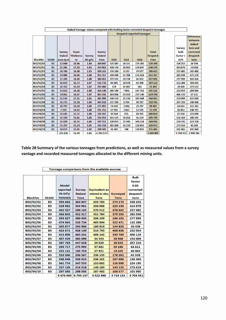
120

Table 28 Summary of the various tonnages from predictions, as well as measured values from a survey vantage and recorded measured tonnages allocated to the different mining units.

121

Table 29 is a summary of the total values, averaged bench thicknesses and relative densities obtained from the reconciliation. Here obvious differences with regard to area, seam thickness, RD and volumes illustrate the disparity in the tonnages reported. Table 29 Summary of the total values, averaged bench thicknesses and relative densities obtained from the reconciliation.

Table 30 Provides overestimation values between the final surveyed derived density as well as the dispatch tons against the model, staked and as mined densities if the geometric parameters of the mined area are set equal to the final surveyed values. Expected tonnages were calculated and compared with the final surveyed and dispatch tonnages to derive the over estimation values.

Table 30 Derived RD based on final surveyed area, seam thickness and volume, illustrating the percentage of overestimation if the model, staked or as mined polygons RD for the same geometric parameters were used.

7.3.3.1 Discussion Volksrust formation mining unit data Data relevant to the mining units selected have been evaluated and comparisons made to determine differences between the different sets of data. The first set of data (Table 24) revealed that the differences between the model values and the staked values were largely due to changes in the mining unit area and slight differences with respect to the mining unit thickness. These differences can be attributed to a difference between desktop planned values and the application of these values to the practical situation with respect to mining operations within the open pit. The

122

mining operation, through drilling, blasting and loading, could be affected by changes in area due to previous mining unit delineations, namely:.

Changes in the back break during blasting increasing or decreasing the volume specified. Changes in roof and floor elevations due to over or undermining of the predicted floor of the

previous mining horizon now representing the roof of the current mining horizon.

The set of comparisons between staked information and the actual mining process in Table 25 shows that the area mined has the greatest influence on the tonnage differences with a minor contribution from the mining unit thickness as a result of either over or undermining of the specified floor. The as mined data is still evaluated on the same relative density values as used for the staked blocks i.e. the raw Archimedes relative density allocated to the specific mining unit. The survey information for the units mined also shows the differences attributable to area and a slightly greater contribution for over or undermining. In such cases, the survey department would make an adjustment to the reported tonnages based on their measurements. Such adjustments, however, would not adjust the assigned relative density values for the specific mining units. The last comparison in Table 27 represents the differences between the staked values and the actual measured tonnages dispatched to the beneficiation plants during the load and haul operation. Truck tallies with assigned tonnage correction factors based on the volume expansion factor for the blasted material and the various trucks carrying capacity are used to denote the actual transported tonnage. This tonnage value can be checked against belt scale values reported for received tonnages at each respective plant, thus it is probably the most accurate measurement that can be relied on in this operation. Finally the total values for each of the five sets of data relating to areas, volumes and tonnages with their corresponding averaged mining unit thicknesses and averaged relative density values were used to evaluate the percentage of over estimation between the model, staked units and actuality are presented in Table 28Tables and Table 29 . For this particular mining unit the percentage of over estimation derived from the evaluation is 17.41% between the model values and surveyed actuality and 17.74% between the model values and run of mine reported by the dispatch system, the actual tons received at the various beneficiation plants. This suggests that the solid matrix represents between 82.26% and 82.59% of the density value depicted by the model, which results in an average geological correction factor of 17.57% for bench 3 mining horizon.

7.3.4 VRYHEID FORMATION DATA Mining horizon 6 or Coal Zone 4 in the Vryheid Formation was selected because it is the only seam that is mined and passed through a crushing and screening plant without any further beneficiation being applied. The raw run of mine material is therefore considered to be representative of the final 100% yield product that is dispatched directly to the power station. The model derived areas, tonnages and bench thickness for the selected mining horizon 6 mining unit polygons are displayed in Table 31. This is the data from which the tonnage evaluation was done.

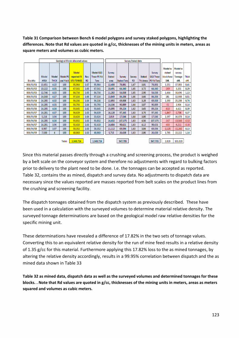
123

Table 31 Comparison between Bench 6 model polygons and survey staked polygons, highlighting the differences. Note that Rd values are quoted in g/cc, thicknesses of the mining units in meters, areas as square meters and volumes as cubic meters.

Since this material passes directly through a crushing and screening process, the product is weighed by a belt scale on the conveyor system and therefore no adjustments with regard to bulking factors prior to delivery to the plant need to be done. I.e. the tonnages can be accepted as reported. Table 32, contains the as mined, dispatch and survey data. No adjustments to dispatch data are necessary since the values reported are masses reported from belt scales on the product lines from the crushing and screening facility. The dispatch tonnages obtained from the dispatch system as previously described. These have been used in a calculation with the surveyed volumes to determine material relative density. The surveyed tonnage determinations are based on the geological model raw relative densities for the specific mining unit. These determinations have revealed a difference of 17.82% in the two sets of tonnage values. Converting this to an equivalent relative density for the run of mine feed results in a relative density of 1.35 g/cc for this material. Furthermore applying this 17.82% loss to the as mined tonnages, by altering the relative density accordingly, results in a 99.95% correlation between dispatch and the as mined data shown in Table 33 Table 32 as mined data, dispatch data as well as the surveyed volumes and determined tonnages for these blocks. . Note that Rd values are quoted in g/cc, thicknesses of the mining units in meters, areas as meters squared and volumes as cubic meters.

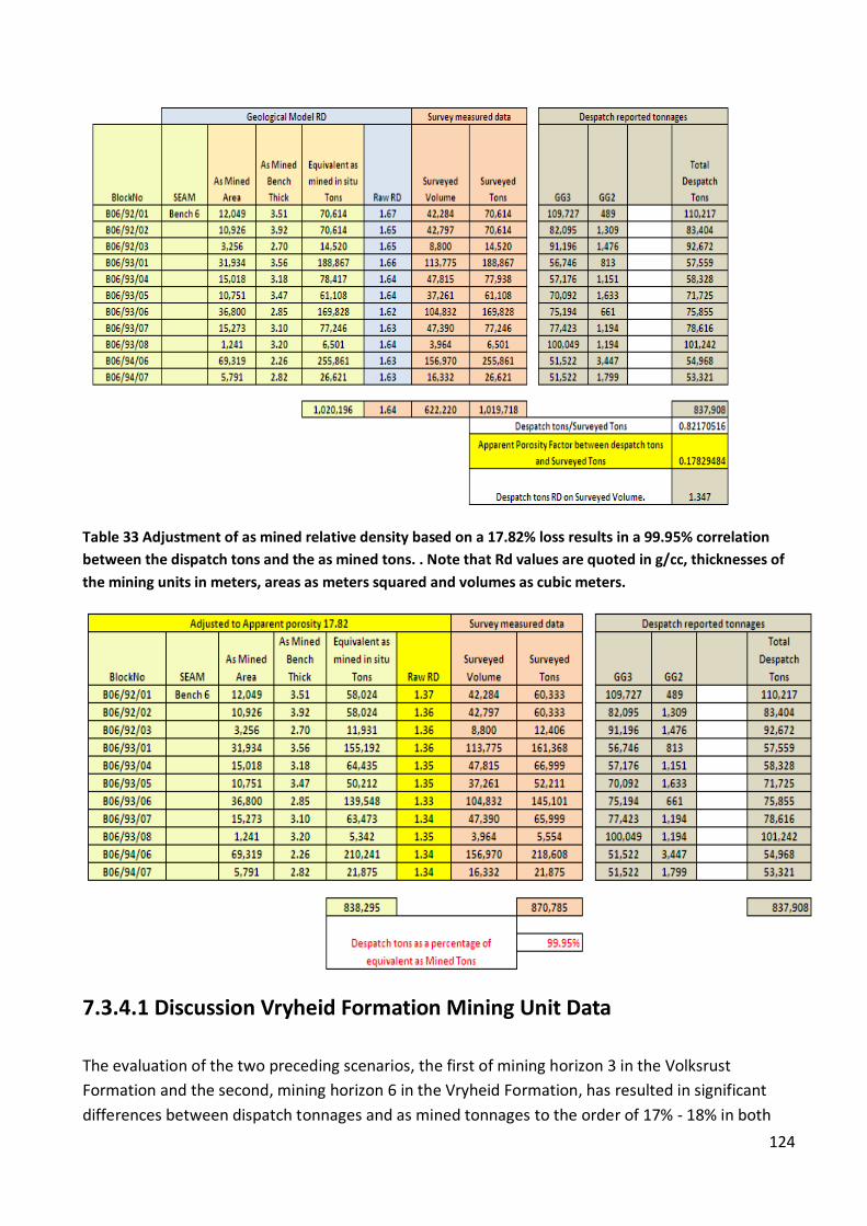
124

Table 33 Adjustment of as mined relative density based on a 17.82% loss results in a 99.95% correlation between the dispatch tons and the as mined tons. . Note that Rd values are quoted in g/cc, thicknesses of the mining units in meters, areas as meters squared and volumes as cubic meters.

7.3.4.1 Discussion Vryheid Formation Mining Unit Data The evaluation of the two preceding scenarios, the first of mining horizon 3 in the Volksrust Formation and the second, mining horizon 6 in the Vryheid Formation, has resulted in significant differences between dispatch tonnages and as mined tonnages to the order of 17% - 18% in both

125

cases. Although the inherent moisture content of most of the samples in the Waterberg succession has been established to be approximately 1.5% - 2.5%, this inherent moisture is structurally trapped within the solid matrix thus forming part of the air dry relative density of the material. If the inherent moisture is taken into account the differences are reduced to approximately 15% which may be representative of the effective porosity of the coal seams. The use of surveyed tonnages and actual reported tonnages resulting in a loss of 17% to 18% from the prescribed predicted tonnages, determined through the application of Archimedes raw relative density values, once again highlights the fact that the Archimedes determined RD cannot be used to determine reserve tonnages. The results obtained from this bench which merely passes through a crush and screen process before being dispatched to the power station validate the overestimation of tonnages from exploration derived data where the Archimedes RD is used for resource and reserve tonnage determinations. The Archimedes determined RD compared with actual results illustrates the extent of the adsorption and absorption of moisture equivalent to the loss percentage during the hydrostatic determination of SG. In this event a geological correction factor equivalent to the loss percentage should be applied to the Archimedes determined RD to align the seam relative density with the density obtained from reconciliation. The corrected density values should then be used for tonnage determinations.

8. RECONCILIATION OF THE BENEFICIATION PROCESS AND BENEFICIATION PRODUCTS.

8.1 BACKGROUND At Grootegeluk Coal Mine three basic types of plant, crushing and screening, single stage beneficiation and double stage beneficiation are in operation. This investigation was initiated for the double stage process producing a semi soft coking coal blend for the mine. A schematic showing the process through the double stage beneficiation plant is shown in Figure 66. The process starts at the source, namely, at the blast block in the mine. Raw feed is trucked to the tipping bins, passed through a Bradford breaker and split into two product streams, one with feed material delivered via screens to two different sets of silos, one for coarse material above a certain size and the other for finer material while the second stream from the Bradford breakers is sent to the discard dumps as waste. Material is drawn from the silos passing through a primary beneficiation stage, resulting in a product for the secondary beneficiation stage, this product is again housed in silos and a waste product from the primary stage is sent to discard. During the secondary beneficiation stage two products are derived, the semi soft blend coking coal and a middlings coal product for the power station.

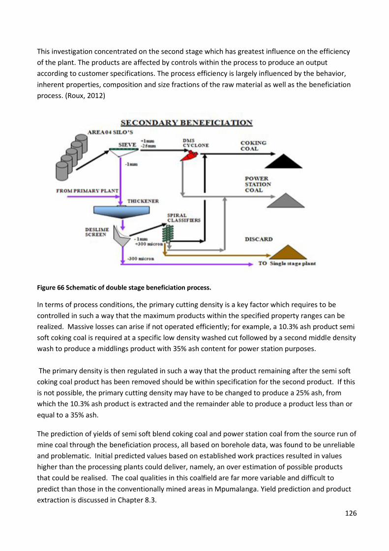
126

This investigation concentrated on the second stage which has greatest influence on the efficiency of the plant. The products are affected by controls within the process to produce an output according to customer specifications. The process efficiency is largely influenced by the behavior, inherent properties, composition and size fractions of the raw material as well as the beneficiation process. (Roux, 2012)

Figure 66 Schematic of double stage beneficiation process.

In terms of process conditions, the primary cutting density is a key factor which requires to be controlled in such a way that the maximum products within the specified property ranges can be realized. Massive losses can arise if not operated efficiently; for example, a 10.3% ash product semi soft coking coal is required at a specific low density washed cut followed by a second middle density wash to produce a middlings product with 35% ash content for power station purposes. The primary density is then regulated in such a way that the product remaining after the semi soft coking coal product has been removed should be within specification for the second product. If this is not possible, the primary cutting density may have to be changed to produce a 25% ash, from which the 10.3% ash product is extracted and the remainder able to produce a product less than or equal to a 35% ash.

The prediction of yields of semi soft blend coking coal and power station coal from the source run of mine coal through the beneficiation process, all based on borehole data, was found to be unreliable and problematic. Initial predicted values based on established work practices resulted in values higher than the processing plants could deliver, namely, an over estimation of possible products that could be realised. The coal qualities in this coalfield are far more variable and difficult to predict than those in the conventionally mined areas in Mpumalanga. Yield prediction and product extraction is discussed in Chapter 8.3.

127

Bulk mining horizon samples from Grootegeluk Mine were evaluated by the CSIR during 1991 and 1992. This work was done to ascertain beneficiation characteristics and derive optimal top sizes for maximum yield especially of semi soft coking coal blends (De Korte, 1992). The results of this exercise were utilized in conjunction with the AAD methodology to derive beneficiation plant specific data which would negate the use of a range of historically applied origin derived correlation factors. (Roux, 2012)

In order to establish the beneficiation characteristics of the Waterberg coals, bulk samples were subjected to a carefully formulated project entailing, sampling, screening and analysis of different size fractions. The results are shown in Figure 67 where the optimal top size (largest particle size) was determined to be < 15mm if all three processes, i.e. Bath type dense medium separation, dense medium cyclone and spirals, were employed.

Figure 67 Schematic reflecting the results of the six subdivided samples at their various top sizes and the beneficiation mediums used for separation.

The standards for laboratory analysis on exploration borehole core samples at Grootegeluk require the core to be broken to -13mm +0.5mm. This is in accordance with the range between -10mm and -15mm. The loss of low ash coal to fines and super fines, however, increases as the top size is reduced and at these low top sizes, the loss at -15mm is less than that at -10mm. The loss at -15mm is approximately 2% while the loss at -10mm increases to 5%+. Therefore the determined top size of -15mm was determined to be the optimal. A baseline for the comparison of ash yield values at various ratios of admixtures from the different mining horizons was determined for material within the >20mm - >25mm range (Roux 2010). This baseline was then used to reflect a probable 100% theoretical yield. Values depicting an 83% yield and a 73% yield were then calculated and plotted to establish a probable correlation curve. These curves are shown on the same plot in Figure 68 and Figure 69 in order to present controls for a

< 150 mm

< 50 mm< 35 mm

< 25 mm< 15 mm

< 10 mm

< 150 mm

< 50 mm

< 35 mm

< 25 mm

< 15 mm< 10 mm

0.00

2.00

4.00

6.00

8.00

10.00

12.00

14.00

16.00

18.00

20.00

0 1 2 3 4 5 6 7Size Fractions

Yiel

ds

Bath type Dense Medium Bath & Cyclone Dense Medium Above & Spirals

128

visual depiction of the resulting yield distribution of various size fractions that could be obtained from this investigation, i.e. relating to material sizes and separation media utilized (Roux, 2010).

Figure 68 represents the baseline regression for material < 25mm top size

Figure 69 Plot of different size fractions behavior in bath, cyclone dense medium and spiral processes compared with yield prediction limits and correlation factor limits.

The foregoing plot in Figure 69 was used to assess the beneficiation process since the plant being evaluated utilized the displayed process. Data from the bulk sample test work showed that feeds in the 25mm to 35mm fractions exhibited a 1.5% to 2% yield improvement, while the 15mm fractions increased dramatically from 4.5% to 12.5% when only the drum and cyclone dense medium separation were used. A further increase in excess of 16% was realized when the spirals were introduced representing another 3.5% increase in yield due to improved liberation of low density material in the smaller size fraction. Most of the low ash coals (i.e. those with ash contents lower than 10.3% ash at 1.338g/cc) are in the density range of 1.305g/cc and 1.334g/cc.

y = 0.0071x3 - 0.0217x2 - 0.4171x + 10.315R² = 0.9931

89

10111213141516

6 7 8 9 10 11 12 13

Yiel

d %

Ash%

Topsize < 25mm Ash / Yield

GG1 Theor Yield for ratio

129

Superimposing plant production results on a template based on results shown in Figure 69, but now depicted in Figure 70 show the highest concentration of consistent results to be greater than 83% on the theoretical predicted yield. An average for the data distribution between ash content controls of 10.2% and 10.4% within the beneficiation environment resulted in a correlation factor of 83% being applied to the theoretical yields in order to make them comparable with actual plant yields obtained. Comparing this with the data from the sized material investigation and the process used, it was established that the products obtained were mostly due to the top size of the feed being < 25mm.

Figure 70 Semi soft coking coal plant yields plotted on template with correlation trends for sized material.

8.2 APPLICATION OF AAD TO PREDICTION OF PRODUCTION YIELDS The ash adjusted density methodology was implemented at Grootegeluk as an aid in improving predictions of products for budgeting and forecasting purposes as well as for the reconciliation of mined and production of products at the end of the value chain. The AAD algorithm and approach were adopted within the grade control environment from early 2008 and used in conjunction with the old format geological model’s theoretical data. Wash tables density data was derived from the AAD algorithm and the subsequent product extractions from these wash tables were done using a 4th order polynomial regression on the cumulative wash table data. This provided more accurate predictions of products from these tables, composited for the respective mining blast blocks being mined. Major comparisons were made between the new ash adjusted density approach values and actual beneficiation plant yields for the material processed. The results were condensed to monthly

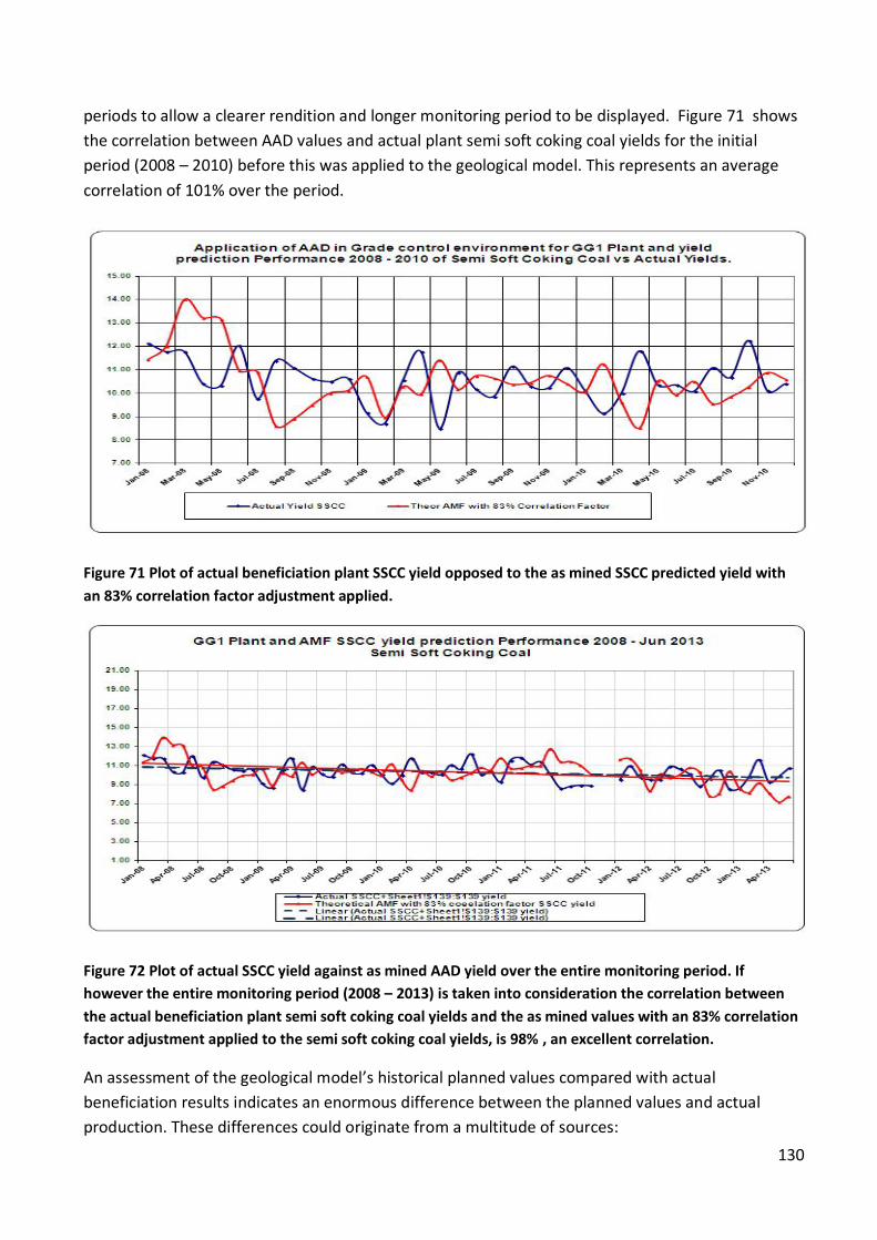
130

periods to allow a clearer rendition and longer monitoring period to be displayed. Figure 71 shows the correlation between AAD values and actual plant semi soft coking coal yields for the initial period (2008 – 2010) before this was applied to the geological model. This represents an average correlation of 101% over the period.

Figure 71 Plot of actual beneficiation plant SSCC yield opposed to the as mined SSCC predicted yield with an 83% correlation factor adjustment applied.

Figure 72 Plot of actual SSCC yield against as mined AAD yield over the entire monitoring period. If however the entire monitoring period (2008 – 2013) is taken into consideration the correlation between the actual beneficiation plant semi soft coking coal yields and the as mined values with an 83% correlation factor adjustment applied to the semi soft coking coal yields, is 98% , an excellent correlation.

An assessment of the geological model’s historical planned values compared with actual beneficiation results indicates an enormous difference between the planned values and actual production. These differences could originate from a multitude of sources:

131

Non compliance with regard to mining units planned and those actually mined. Differences in the tonnages of the respective units having been determined from recorded raw

density values used in the geological model.

The methods of extracting products from the standard wash tables, where the fractions are related to specific density ranges with no attempt being made to ascertain the true density of the float fraction and relating this to the initial mass of the samples. Eg. Material that floated at 1.35g/cc, may have a true density substantially lower. A high volatile bituminous coal may have a true density as low as 1.25g/cc or it could be equivalent to the highest value in the range being 1.35g/cc in this case.

Initial masses from a mining environment are compared to an analytical environment. In an analytical environment the mass of the total sample as well as the masses of each float fraction are known, thus a yield value obtained is related to the mass of that specific fraction and the total mass of the sample. Tonnages given for a specific mining unit are based on the raw in-situ density of the unit and not from actual measured mass of the feed material

The geometry of the unit may be different as a result of over or under mining of the preceding overlying unit.

Theoretical product extraction methods from the analytical wash data.

Figure 73 Historical geological model planned SSCC yields and actual beneficiation plant SSCC yields.

Figure 73 illustrates the difference which gave rise to the initial research mentioned. Results obtained from the initial investigations and comparisons eventually led to a partial acceptance of the application of ash adjusted density which in turn allowed the reconstruction of the geological model based on ash adjusted data.

132

The 2010 geological model was built using the ash adjusted theory and implemented to run concurrently with the old geological model from March 2011. Using the same criteria as above, the gap shown in Figure 74 has now been reduced to approximately 3%.

Figure 74 Historical model yields as well as revised geological model yields obtained through the application of ash adjusted density compared to actual plant yields.

Figure 75 Geological model planned yields against actual plant production and the as mined ash adjusted density yields with an 83% correlation factor applied.

The beneficiation plant used for these comparisons is a double stage process as shown in Figure 66. Here a primary cut is taken at a set relative density so that the product remaining after the semi soft coking coal product at 10.3% has been extracted is still within specification with regard to power station coal requirements. This product is referred to as a middlings product. This middlings product is also susceptible to prediction variations as a result of possible misplacement of coking coal to middlings or vice versa and invariably results in a yield percentage higher than predicted. Figure 75 illustrates the differences between the three sets of data, the geological model yields, the actual plant yield and the as mined yields.

133

Figure 76 Plots of the same three measured parameters for power station coal over the period of interest.

Although the initial evaluation into the composition of the coal [with relevance to maceral type and distribution as well as material feed top size and liberation of required products] all contributed to an improved and more acceptable prediction for the expected products and gave credible results comparable with actual beneficiation plant production, the methodology still displayed some inexplicable shortcomings. Plant specific correlation factors for the required products were still required. The most important aspect when reconciling plant output was found to be that the primary analysis, i.e. proximate analysis, had to be conducted on the 13mm+0.5mm air dried fraction. Determined tonnages, based on the wash data from these analyses must be adjusted to take into account the differences between relative densities determined for this -13mm material and the original relative density used to determine the run of mine feed to the plant. This is necessary whether the raw density was derived via the Archimedes principle, the raw field masses or by set laboratory standard procedures such as the Australian Standard method, into account. An average loss factor of 17.82% was determined from a re-assessment of data relevant to the run of mine budgeted tonnages and actual reported run of mine tonnages obtained from monthly reconciliation data monitored as part of the grade control process. Considering the foregoing statement, this loss factor was not identifiable based upon origin and cause, but was based on the reconciliation of budgeted data against the AAD determined data. This factor was then applied to the condensed monthly reported data to assess the overall effect on the re-evaluated run of mine and associated production of both semi soft coking coal and middlings products. This allowed similar comparisons to validate this factor. The first of these comparisons, as shown in Figure 79, was applied to the run of mine tons reported, reducing these to an effective air

134

dry state from which was then calculated new semi soft coking coal yields over the monitoring period. The adjustment resulted in a 2% increase in semi soft coking coal yield values.

Figure 77 Beneficiation plant yields as reported based on reported tonnages compared with an applied loss factor adjusted run of mine tons and the concomitant yields.

If this new adjusted value is superimposed on the planned theoretical yields for this period. The latter part of Figure 78 correlates very well with the theoretical planned yields.

Figure 78 Adjusted plant yields compared with planned theoretical semi soft coking coal yields.

Differences as shown in Figure 76 are attributable to deviations with respect to units mined as compared to units planned and the ratios of these units per mining horizon as well as fluctuations with regard to ash content controls within the plant, but the overall fit of the trend is more credible from March 2011 to April 2013. The variations mentioned earlier, especially the ash specifications used for the density of separation control within the beneficiation process, have a major impact on yields. It should be noted that the

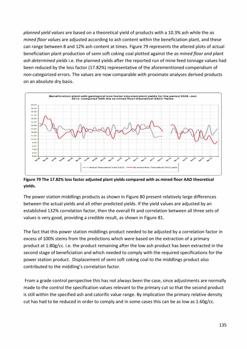
135

planned yield values are based on a theoretical yield of products with a 10.3% ash while the as mined floor values are adjusted according to ash content within the beneficiation plant, and these can range between 8 and 12% ash content at times. Figure 79 represents the altered plots of actual beneficiation plant production of semi soft coking coal plotted against the as mined floor and plant ash determined yields i.e. the planned yields after the reported run of mine feed tonnage values had been reduced by the loss factor (17.82%) representative of the aforementioned compendium of non-categorized errors. The values are now comparable with proximate analyses derived products on an absolute dry basis.

Figure 79 The 17.82% loss factor adjusted plant yields compared with as mined floor AAD theoretical yields.

The power station middlings products as shown in Figure 80 present relatively large differences between the actual yields and all other predicted yields. If the yield values are adjusted by an established 132% correlation factor, then the overall fit and correlation between all three sets of values is very good, providing a credible result, as shown in Figure 81. The fact that this power station middlings product needed to be adjusted by a correlation factor in excess of 100% stems from the predictions which were based on the extraction of a primary product at 1.80g/cc. i.e. the product remaining after the low ash product has been extracted in the second stage of beneficiation and which needed to comply with the required specifications for the power station product. Displacement of semi soft coking coal to the middlings product also contributed to the middling’s correlation factor. From a grade control perspective this has not always been the case, since adjustments are normally made to the control the specification values relevant to the primary cut so that the second product is still within the specified ash and calorific value range. By implication the primary relative density cut has had to be reduced in order to comply and in some cases this can be as low as 1.60g/cc.

136

Figure 80 Theoretical, as mined and actual power station coal yield based on adjusted ROM tonnages.

Figure 81 Beneficiation plant power station coal adjusted with a 132% correlation factor determined from historical data starting in 2008 to April 2013.

8.3 MINING UNIT YIELD PREDICTION AND DATA EXTRACTION FROM WASH DATA Each mining unit of specified proportions needs to be drilled and blasted. The blast drill holes are geophysically logged so that the vertical sequence through the mining horizon can be identified and related through correlation to the exploration boreholes and to samples and/ or portions of samples specific to that horizon. Quality parameters need to be determined for these spatially representative holes in order to obtain data to establish a workable washability table for the material from that specific mining unit. It is this that would provide the anticipated material to be processed by the different beneficiation plants. This is correlation is accomplished through mini modeling. The information garnered from

137

the blast-hole positions in each specific mining block is condensed into a representative wash table for the entire mining unit, provided that the vertical section is relatively constant for the unit. This protocol was followed before AAD was developed and it has not changed since the introduction of AAD. The fixed range densities determined from the wash tables were adjusted to provide apparent density values for the individual float fractions according to the densities derived from the AAD algorithm therefore the extraction of products as well as the interpolation of data within the framework of this table has changed. Earlier methods of extraction as promulgated in the 1980’s were based on methods which were purported to improve accuracy for semi soft coking coal yield and quality. These methods using the old French curve fit as a basis for comparison, were expanded, tested and proven adequate at the time for conversion to computer generated methods of extraction. But these were only applicable for semi soft coking coal in the 8% to 12% ash range (de Lange, 1986.) The method used was named SPR by the designers of the software written for MSDOS based applications. Consider the following example of a mining horizon unit with a fractional wash table from which product extraction at specified ash contents is predicted. See Table 34. Table 34 Fractional wash table proximate data for a potential mining horizon 2 mining unit.

Note however that the values in this table still need to be cumulated so that product extraction can be done.

138

Table 35 The cumulative wash table of fractional values in Table 34.

In Table 34 Fractional wash table proximate data for a potential mining horizon 2 mining unit.the starting ash value of 10.39% at the 1.35g/cc float range is slightly higher than the equivalent ash content of 10.3% required for a semi soft blend coking coal product. Due to the configuration of the computerized SPR extraction of products at these different values, no semi soft coking coal product is shown at the 10.3% ash content value in Table 36 Template from an excel program written to do product extraction from wash table data reflecting the calculated values for the products requested for these specific beneficiation plants., although in the original wash table, Table 34 Fractional wash table proximate data for a potential mining horizon 2 mining unit. a yield of 11.28% at 10.391% ash content is shown. This is due to the fact that the SPR extraction requires two data points for the evaluation method to work, one higher than the value sought and one lower than the value sought. It then computes a logarithmic interpolation between these points to extract a theoretical product. No semi soft coking coal product can be extracted in this actual case, because the ash content is higher than the 10.3% ash content specified. This program also cannot provide a value for a middlings product.

139

Table 36 Template from an excel program written to do product extraction from wash table data reflecting the calculated values for the products requested for these specific beneficiation plants.

Table 37 Float / sink wash table with the densities changed due to the application of the AAD algorithm on the original float densities.

Table 38 the cumulative densities of AAD adjusted Table 37

140

The second part of this example uses data from the wash table as seen in Table 38 with the AAD determined densities of the float fractions, shown as individual values for the proximate ash contents at each specific density. The reflected density represents the density at which the run of mine feed must be cut (sink/floated) in order to obtain the required product. Table 38 the cumulative densities of AAD adjusted Table shows the cumulative densities as the ash content increases. The final density would be equivalent to the absolute dry density of the solid matrix of the sample, since this is an accumulation of all the float values as well as the final sink value. The template in Table 39 provides product information according to the required specifications. Note that the calorific value for GG2 (the power station coal) at 35% ash content is out of specification with a calorific value of 16.73Mj/kg. The lower cut density at 1.90g/cc will suffice to produce the required product. Table 39 Template reflecting the calculated values for the products sought in the left hand columns for these specific beneficiation plants derived from the AAD cumulative wash table.

Extraction of data from this wash table, although it can be done using the SPR method, is based on a 4th order polynomial and all the expected values have been calculated from the resultant curves generated relative to the density requirements. This method of extraction has been modified so that only interpolation within the data range can be done. Although the foregoing is a single example of a representative block/mining unit’s wash table and the products that can be extracted, it is quite clear that a better estimate of the expected products is obtained using the ash adjusted density methodology. This method also allows the user to adjust the cut (sink/float) specifications so that the best predictive solution can be obtained. Proof of the accuracy of the interpolation method is shown in

141

Figure 82. Here the data from the wash table has been used to generate a cumulative plot, and trend lines with respect to three extraction methods have been incorporated in this plot. i.e.

A logarithmic fit for values up to a 35% ash content value The Lagrange trend fit, equivalent to a 3rd order polynomial Cubic spline generated data points as shown in the table next to the plot.

Figure 82 Wash table curve fitting trends for interpolation of yield values at specified ash content.

The closest trend fit to the historical hand drawn French curve fit for the direct evaluation of ash content plotted against yield on graph paper is a cubic spline interpolation of the basic point data in the cumulative wash curve. The fundamental principle behind the cubic spline interpolation is the generation of a smooth curve through a number of data points. The coefficients generated on the cubic polynomials used to interpolate the data, bend the trend line so that it passes through each of the data points without any erratic behavior or breaks in continuity. One of the main advantages of the cubic spline’s application is the ability to correlate data and extract interpolated values between data points which do not follow any specific pattern without a single polynomial’s extreme behavior. (McKinley et al, 2005)

142

The grade control approach thus is more flexible and is particularly important when several mining units are planned at predetermined ratios. Comparisons between the planned values, the as mined values and actual beneficiation plant results can then be done. The foregoing plots at the beginning of this chapter pertaining to this, over the monitoring period starting in 2008, clearly show the differences, not only with regard to actual products derived, but also the effect of non-adherence to planned ratios and ash contents within the beneficiation environment. This controversy is illustrated in the example shown in Figure 83 where the uppermost plot portrays the planned ratios of the various benches to the beneficiation plant. The second plot in the middle of the diagram depicts the actual ratios of material delivered to the plant from the mine, clearly, mining are not conforming to the planned execution to ensure the required production. The last plot depicts the deviations from planning.

Figure 83 Combination plots of daily feedstock to the beneficiation plant.

The beneficiation plant’s varying response to the received feedstock and the controls exercised within the beneficiation plant for the same period are illustrated in Figure 84. Figure 84 portrays two plots, namely the semi soft blend coking coal yield comparisons between the as mined yields

143

and the actual plant yields as well as the ash content controls utilized during this period. In the second plot the power station coal production with the same elements considered, are shown. It will be noted that, in many cases, total middlings yields are substantially higher than those initially predicted. This is likely to be due to misplacement of semi soft coking coal to the middlings products as well as recovered slimes being added to the product beds. An evaluation of the total yields, i.e. the sum of semi soft coking coal and power station coal, however shows minimal variation to approximately February 2012. This supports the assumption regarding the misplacement of the semi soft coking coal to middlings.

Figure 84 Combined plots of monthly SSCC and PS coal production compared with plant ash content.

From February 2012 fluctuations are mainly associated with actual run of mine material to the plant and also linked to changes in product demand mostly for power station coal. A lower ash obtained for power station coal during beneficiation as a result of lower ash semi soft coking coal, also prompts an increase in the primary cut density above the 1.80g/cc predicted value which will result

144

in higher power station coal yields. Overall, an increase from approximately 40 to 45% total yield is noted over this period as shown in Figure 86.

Figure 85 Plot of total yields for the monitoring period.

Figure 86 Trend of total yield over period increasing from approximately 40% to 45%.

8.3.1 Discussion The information used in earlier research conducted by the author and reported in his 2012 dissertation relating to the optimal yield and cut density prediction of semi soft coking coal and power station coal in the Waterberg coalfield has been re-visited. The plant specific correlation factor determined there, i.e. 17.82%, which was originally used to address the difference between plant products and planned values, has been used on the reported run of mine tonnages in this

145

current research programme in an attempt to gauge the effect of this application with respect to the actual reported tonnages along the value chain. The original application demonstrated an improvement in yield predictions but could not justify the total loss; i.e. some 12% -14% could not be accounted for in the original dissertation. The application of the loss factor as established in this current study, however, has significantly improved the correlation between the planned and actual values in terms of mine tonnages reporting to the wash plant. The plant specific correlation factor determined between actual reported tonnages and the predicted values has therefore been validated. This factor includes plant efficiency and losses attributable to incorrect tonnages reported. The tonnages used in these reconciliations represent the final monthly reported tonnages after survey adjustments had been made. The reported loss in respect of coking coal tonnages portrayed by the correlation factor however is more applicable to the reported run of mine tonnage. An example included in Table 1Table 40 shows a correlation factor of 88.3% based on actual production against geological model yields. Table 40 Reported plant tonnages vs AAD geological model predicted yields for the period January 2014 to December 2014.

When the loss factor of approximately 12% in this case was applied to the reported run of mine tonnages, and then compared with the AAD predicted geological model values, an excellent correlation as depicted in Table 41 was achieved.

146

Table 41 Run of mine tons reported by beneficiation plant adjusted by a geological loss factor of 12% compared with AAD geological model predicted yields.

147

9. GRADE CONTROL VIA DOWNHOLE GEOPHYSICAL LOGGING This Chapter seeks to validate the approaches reported above with respect to the actual in situ nature of coal, i.e. to prove by means of geophysics the true nature of coal in its natural state in terms of density, moisture content and porosity.

9.1 LOG EVALUATION FOR SOLID MATRIX DENSITY AND PROBABLE EFFECTIVE POROSITY DETERMINATION The main objective of the utilization of down-hole geophysical measurement is to determine and quantify in-situ the inferred density, moisture holding capacity or effective porosity of coal which could influence the values derived for the raw material. More specifically, this is to determine and validate tonnage derivations for resource and reserve estimations. In evaluating a coal sample’s physical attributes, the solid matrix and the contribution of the voids, whether fluid, air or gas filled is generally ignored in the initial stages of exploratory work conducted in the field, to the detriment of density calculations used for tonnage estimates. Coal is characterized by a dual porosity, which consists of micro-pore and macro-pore systems. The micro-pore system is estimated to have pore diameters less than 2 nm, which occur as part of the coal matrix. The macro-pore system is established by the fracture network that is currently designated by the cleat system (Van Krevelen, 1993). Other discontinuities that contribute to the macro-pore system are the bedding planes or surfaces. Physical factors, such as compaction and water expulsion, progressively reduce porosity. The development of secondary porosity begins with the formation of meso-and micro-pores at approximately the ASTM Designation D388-98a for low volatile bituminous coal. This implies an increase of porosity due to well-known progressive changes in the molecular structure through higher ranks. Porosity is also related to the maceral composition. Vitrinite predominantly contains micro-porous contents, whereas inertinite predominantly contains meso and macro-porous contents (Gan et al., 1972; Unsworth et al., 1989; Lamberson and Bustin, 1993; Levine, 1993). As a result of the controversy surrounding the raw relative densities used for tonnage estimations, alternative methods in line with SANS guidelines were evaluated in this research program. The reason for doing so arose because conventional methods used to calculate tonnages in the mining industry have provided values that are questionable. The conventional methods determine tonnages via the Archimedes principle, and, based upon the current research, the credibility of such a method is in doubt and indeed seriously misleading. A project re-logging existing exploration boreholes with Auslog dow-hole geophysical logging sondes was underway during the course of the current research and this provided an opportunity to undertake advanced evaluation of the nature and form of coals as they exist in situ. The purpose

148

was to obtain information from which to interpret the solid matrix density and the measured bulk density of the coals in their various seams. In situ adventitious moisture or effective porosity was also determined. The results were used to determine (i) the loss factor on the calculated tonnages and (ii) an adjustment to the raw density to represent an equivalent density of the matrix which could then be used for tonnage derivation.

9.2 REVIEW OF GEOPHYSICAL LOG INTERPRETATION METHODOLOGY Four basic geophysical logs were initially obtained from one combination geophysical tool, i.e. natural gamma, dual density-Long spaced density (LSD), Short spaced density (SSD) and a single arm calliper trace. The SSD and LSD raw counts per second were converted to apparent density using site specific calibrations based on empirical data related to sample densities from laboratory data. The density and associated counts per second for water were also included in the calibration regressions. The calliper log was not calibrated, but served to indicate areas of possible caved sections. The natural gamma log was evaluated to indicate a shaliness index or very broad based clay content. Empirical data derived from ash determination of the coal and shale samples from the Waterberg Coal Field were noted. Grootegeluk evaluation: ℎ = * 0.90

The result of this equation is deemed to represent the shaliness index of the coaly or rocky interval being evaluated. This in turn was then used to be representative of the ash content (indestructible mineral matter) of the sample. The mineral matter of the coal samples in this coalfield consists mainly of quartz and kaolinite clay with other minor mineral and trace elements. The 0.90 factor was derived from an average ‘low ash’ of 6% and a ‘maximum ash’ of 96%, the remaining 4% representing material lost on ignition during XRF analysis. Schlumberger (Log interpretation principles, 1969) suggests that, if the radioactivity level of the clay is constant and no other mineral in the formation is radioactive, the gamma ray reading after correction for borehole conditions may be expressed as a linear function of the clay content: GR = A +B V clay Then the formula can be written:

=( − 1( 2 − 1)

Where γ1 represents gamma readings in clean intervals and γ2 represents gamma readings opposite clay beds. If radioactive minerals other than clay are present, the indication derived from the gamma ray will be too high. As the Grootegeluk equation was derived from empirical data, this equation has been applied in the evaluations. A pseudo density, representative of the probable solid matrix was determined by applying the AAD algorithm, or conversely, the shaliness index which was used in an equation using the petrophysical densities pertinent to the composition of the

149

sample, i.e. (The shale to coal ratio). The pseudo density value was then determined by applying the AAD equation (0.013*ash+1.2384) where the ash content is equivalent to the derived shaliness index value. Knowing the shaliness index percentage allowed the determination of the coal content. A matrix density could thus be determined using the petrophysical densities for bituminous coal which is approximately1.24g/cc and quartz/kaolinite shale which is approximately 2.53g/cc. The effective porosity was then determined by the equation:

∅ = 1 − ( )

The correction was applied to the SSD which represents the bulk density of the formation being measured utilizing the derived porosity value to accommodate possible voids, irrespective of whether they were air or moisture filled. This was obtained by adjusting the SSD value according to its determined compositional contribution. Example, 18% porosity on a total bulk density of 1.80g/cc would essentially be 1.80g/cc*0.82=1.476g/cc. The logical conclusion evaluating the bulk density against the probable matrix density could give two possible results, i.e. (i) if the matrix density is less than the bulk, the increased value representing the bulk density can be attributed to moisture within the matrix while (ii) a reversal of this, implying a higher matrix density than the measured bulk density, would imply air or gas filled voids. The geophysical log traces and conversions to evaluative data are illustrated in Figure 87, 88 and 89.

Figure 87 Geo-log extract with accompanying NG trace on the left and a comparison between the SSD with calculated matrix density on the right, the yellow trace representing the inferred matrix density and the turquoise trace representing the interpreted bulk density. The measured ground water level at the time of logging this borehole is also shown.

150

Figure 88 Overlay comparison of NG pseudo density on SSD apparent bulk density. The NG trace, far left, apparent bulk density next and the last column representing the overlay of the apparent density on the inferred matrix density.

Figure 89, effective porosity or moisture holding capacity compared with SSD density and Matrix density.

151

9.3 EVALUATION OF A SELECTED SECTION OF EXPLORATION BOREHOLES A series of exploration boreholes in closest proximity to the western face advance were selected for a trial investigation. The geophysical logs of each borehole, HT30, HT75, GK104, GK86, GK102, GK114 and GK101 are depicted in Figure 91 Line of section of exploration boreholes logged The logs and interpretive logs depicted are in column 1, an interpreted porosity log, column 2, an interpreted matrix density overlaid on the short spaced density representing the measured bulk density of the in situ formation. The first of these boreholes, GK86 is expanded in Figure 92 to display some detail in the upper portion of the borehole, i.e. two deviations on the caliper trace indicate possible caving, however, minimal yet sufficient to portray lower bulk density values. The matrix density on the other hand derived from the natural gamma log also gave a very low corrected density value which supports the low bulk density value obtained, thus negating the effect of the possible caved material.

Figure 90 Locality map of section chosen for geophysical examination of borehole logs.

152

Figure 91 Line of section of exploration boreholes logged, the log traces in each following the same protocol described, inferred porosity and inferred matrix density overlain by the interpreted bulk density. This also illustrates the correlation of the Volksrust and Vryheid Formations across this line of section.

153

Figure 92 is he expanded section of GK86, showing on the left a table of information relative to sample depths, zone classification, representative bench, the raw RD per sample, composited RD per bench, inferred porosity SSD log bulk density and the corrected RD based on the inferred porosity. The log traces shown are caliper, inferred porosity and a combination of the inferred matrix density the porosity corrected density overlain. Cross-overs where the corrected density is lower than the bulk density are shaded in blue.

154

The 7 boreholes were evaluated to determine (i) a pseudo density from the natural gamma log (ii) an effective porosity value (iii) and a corrected relative density based on the foregoing information. The averaged results representing the different mining benches are shown in Table 42 below. These averaged values suggest that an overall average porosity of approximately 14% for the Volksrust formation may be acceptable for estimation purposes.

Table 42 Averaged density values for the 7 exploration boreholes evaluated.

Note 1: sample 1a is excluded in this calculation since it is considered as waste with the overburden. The reason for the exclusion of sample 1a being that there is a 1.5m to 2m thick carbonate enriched shale separating this seam from the rest of bench 2. This thick shale bed dramatically reduces the yield of bench 2 material; therefore it is selectively removed with sample 1a when the overburden is stripped. Note 2: benches 2 and 3 are affected by weathering, thus the full succession of samples in the vertical sequence is not present in all the boreholes, and this will also result in fluctuations in values. The grouping of tables in Table 43, reflect the analyses done from which the averaged values in Table 42 were obtained.

Table 43 Summary of values obtained for the individual benches in the exploration boreholes.

156

A geophysical re-assessment of borehole MY23 was chosen to validate the evaluation of the averaged densities determined from the exploration boreholes used in the line of section chosen in the foregoing evaluation. This core was chosen because extra data with respect to densities obtained in the laboratory per float fraction was available on this particular borehole. This data was used to examine /establish the accuracy of the AAD methodology. This borehole was also chosen because the greatest part of the coal succession is below the groundwater table, thus it is reasonable to assume that (i) most of the lithological units capable of storing adventitious moisture would be saturated and (ii) the in-situ density would thus be a combination of the rock plus coal matrix density and moisture. The ground water table was approximately 38m below surface when this borehole was geophysically logged.

Figure 93 Bench 2 geophysical log evaluation for inferred porosity shown in the first trace and the interpreted bulk density overlying the inferred matrix density in borehole MY23.

The information in Table 44 is of great value since a reasonable correlation between the geophysically determined effective porosity and the effective porosity determined from the -13mm air dry density related to the volume of sample, especially in the vitrinite rich Volksrust Formation for B2-B5, exists. Furthermore the correlation between the Archimedes determined SG and the geophysically derived short spaced density, is also very good, the differences being in the second decimal in most cases. Only bench 11 values do not correlate, the Archimedes SG being substantially lower. This could be attributed to insufficient moisture saturation during the hydrostatic SG determination of the sample.

157

Table 44 Summary of evaluated data for MY23.

Figure 94 provides a summary of the values obtained from the geophysical log interpretations and a comparison of results obtained from the evaluated boreholes on the line of section and results of the same bench configurations for the benches in borehole MY23. The bar graph clearly illustrates a decrease in porosity from bench2 at the top of the succession (B2) to bench 5 (B5) at the base of the Volksrust Formation. This is directly related to the distribution of vitrinite rich coals with micro-porosity within the Volksrust Formation, with the best samples concentrated in bench 2 at the top of the vertical succession. Bench 6 displays higher porosity values than bench 5 due to increased macro porosity associated with the maceral composition of bench 6 which is inertinite rich. Bench 7a and bench 8 are essentially waste benches, while bench 7b portrays a relatively poor quality coal also inertinite rich. The remaining coal seams, bench 9a, 9b, 11 and 13 display increasing porosities as the inertinite content and macro-porosity of the seams increases. These lower seams display a variation between 14% and 18% porosity. Comparisons for bench 8 and 9a could not be made since bench 9a has been replaced by channel sandstone in borehole MY23, only the lowermost sample; sample 29 of bench 9b is present in MY23.

158

Figure 94 Is a compilation of (i) a bar plot comparing the average derived effective porosity for the benches evaluated in the line of section and the porosities determined for the control borehole MY23 and (ii) a plot of average porosity corrected Archimedes densities from the boreholes in the line of section with MY23 porosity corrected density values for the individual benches. The variance between the two datasets is smaller than 0.2g/cc.

The final plot in Figure 94 shows the comparison of sample densities corrected to a solid matrix density by taking the determined porosities into account. The statistics done on the differences between the two datasets compared in this evaluation illustrates a very good correlation between them at a 95% confidence level.

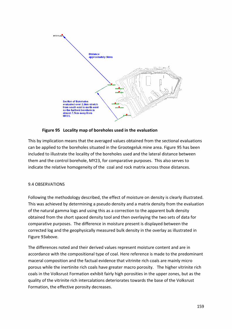
159

Figure 95 Locality map of boreholes used in the evaluation

This by implication means that the averaged values obtained from the sectional evaluations can be applied to the boreholes situated in the Grootegeluk mine area. Figure 95 has been included to illustrate the locality of the boreholes used and the lateral distance between them and the control borehole, MY23, for comparative purposes. This also serves to indicate the relative homogeneity of the coal and rock matrix across those distances.

9.4 OBSERVATIONS Following the methodology described, the effect of moisture on density is clearly illustrated. This was achieved by determining a pseudo density and a matrix density from the evaluation of the natural gamma logs and using this as a correction to the apparent bulk density obtained from the short spaced density tool and then overlaying the two sets of data for comparative purposes. The difference in moisture present is displayed between the corrected log and the geophysically measured bulk density in the overlay as illustrated in Figure 93above.

The differences noted and their derived values represent moisture content and are in accordance with the compositional type of coal. Here reference is made to the predominant maceral composition and the factual evidence that vitrinite rich coals are mainly micro porous while the inertinite rich coals have greater macro porosity. The higher vitrinite rich coals in the Volksrust Formation exhibit fairly high porosities in the upper zones, but as the quality of the vitrinite rich intercalations deteriorates towards the base of the Volksrust Formation, the effective porosity decreases.

160

After the transition from the Volksrust Formation to the Vryheid Formation in zone 5, the porosities in the underlying coal seams of the Vryheid Formation increase downwards towards the base of the coal bearing seams ending in zone 1 at the base. This seam exhibits the highest porosity in the lower portion of the Vryheid Formation and also produces a high grade metallurgical coal. The three basic geophysical probes used for this evaluation are adequate to provide a reasonable comparative basis against which physical measurements in the field and preliminary measurements with regard to sample preparation as well as laboratory analysis can be made. i.e.

A properly calibrated density probe gives a reliable apparent bulk density value for the lithologies intersected. This value can safely be assumed to represent the in-situ bulk density of the strata logged.

The calliper probe gives an indication of the boreholes rugosity, thus aiding the interpretation of the density data in areas where caving may have occurred and the source and detector portion of the probe were not properly engaged with the sidewall of the borehole resulting in an air gap which could also contain water if this were below the groundwater table. In such a case the calliper probe needs to be calibrated as well so that the correct diameter of the hole can be measured and the interpreter could then take this into account in determining the true density of the formation being measured.

The interpretation of the natural gamma log after de-spiking and normalization allows the determination of a pseudo density derived from the AAD algorithm, where the shaliness index is used as a possible ash indicator representative of the indestructible mineral matter in the coal samples.

This same shaliness index is also used in a petrophysical calculation to represent a predetermined relative density for this material in combination with the accepted petrophysical density of bituminous coal resulting in a representative value for the solid matrix of the sample.

The difference between matrix densities expressed as a percentage of the pseudo density can then be accepted as being representative of either adventitious moisture content or apparent effective porosity.

The bulk density determined from the short spaced density log is then corrected to provide a representative dry matrix density for the interval of interest.

The bulk density obtained from the geophysical logs is more representative of the in situ density of the succession being logged than cored intervals that have been recovered during exploration, laid out for geological visual logging and description, allowed to become partially air dried and then sampled before the Archimedes density determination for the sampled intervals is done.

If the matrix density values were adjusted to include the inherent moisture and then used as a representative air dry density for tonnage estimations on an air dry basis, the resource and derived reserve values may be more credible.

161

This additional approach complementing existing evaluations has been validated through the comparison of special analyses conducted on borehole MY23 where the ash adjusted density values were compared with pycnometrically (density bottle) determined densities for the float fractions of the samples analyzed. In this case, the volumetric component is once again deficient because no information relevant to the moisture holding capacity or effective porosity is available, thus the samples could not be reconstituted to their original state. A partial solution through the evaluation of down-hole geophysical logs in determining a matrix relative density based on the composition of the sample in respect of the coal to mineral content ratio and adjusting this to accommodate inherent moisture content has provided a baseline from which effective porosity or moisture holding capacity can be determined. Provisional reconciliation data from the mining operation conforms to the losses related to the differences between the theoretically determined tonnages using the Archimedes determined relative densities and actual plant received tonnages. Further proof of the accuracy of these values can be attained through whole core helium pycnometry.

162

10 SUMMARY OF DEVELOPMENTAL AND TEST WORK This chapter summarises the developmental, analytical and validation work undertaken in this thesis. The intent of this thesis was to formulate an applicable philosophy through the re-evaluation and refinement of the previously developed ash adjusted density methodology and to extend its application, in order to provide more credible, reconcilable data applicable to resource and reserve evaluation throughout the entire value chain. Comparisons of the original data with re-evaluated data after laboratory analysis had been received has provided an improved evaluation of the original data and validated alternatives that could be considered should the original data or determinations appear suspect.

The AAD values represent a good approximation of the true dry density of the solid matrix. Add the inherent moisture percentage to this and the resultant density should be

representative of the density of the matrix of the air dried sample. It should be noted though that this density value is also related to a reduction in the original

volume of the sample as a result of milling to a particulate size for analysis. If the mass of this milled product and the original geometric volume of the core sample

were used in the basic density equation, a density value less than the AAD, pycnometer or Archimedes value would be obtained.

This value represents the air dried density of the original core sampled. The difference between the two values would then be representative of either free

moisture, moisture holding capacity or effective porosity.

10.1 A series of sequential research tasks were undertaken. The following points summarize them and their outcomes. The re-evaluation and refinement through descriptive statistics of the ash adjusted methodology and concomitant proof in the application of the derived algorithms obtained from regression analysis of 31,000 datasets compares favorably with density values determined using the Australian Standard method for each float fraction for all the samples analyzed in the borehole used for comparative purposes. Points to note:-

The refinement here relates only to the solid component of the samples because the original state of the samples analyzed in the laboratory has been volumetrically changed.

The samples were crushed to -212µm and dried, therefore any effective porosity would have been destroyed and the volume of the sample would have been substantially reduced from its original state.

The regression analysis determined a constant representative of the incremental mineral content reflected by the product of this and the ash% content while the intercept represents the density of bituminous coal.

163

This last value corresponds with petrophysical analysis done by Schlumberger; they proposed a matrix density for bituminous coal of 1.24 g/cc. The value obtained from the regression analysis is 1.2384 g/cc, rounded up, 1.24 g/cc.

An alternative proposed by Robeck and Huo determining mineral matter content which was proposed to be more accurate than using the ash content referred to as residual mineral matter after combustion, was also evaluated to ascertain the difference between the two. Their methodology (Appendix A) was followed up to the application of estimated in situ moisture, at this stage, with no valid information available, the value for inherent moisture and the matrix density of bituminous coal and mineral matter previously determined, was used so that an air dried density could be obtained. This air dried density could then be compared with air dried density values obtained from the AAD method as well as basic mass/volume determinations on the sample material. Correlations between the various methods are summarized in Table 45 Summary of correlations between the Gray method, AAD, Density bottle and inherent moist adjusted AAD. Note that the reference 1 is applicable to the method, while the decimal value denotes the correlation. Table 45 Summary of correlations between the Gray method, AAD, Density bottle and inherent moist adjusted AAD

The adaptation of AAD can now be used to:

Validate petro-physical properties relating to the matrix density of bituminous coal used by industry.

Assist in the evaluation and type characterization of coal encountered through the evaluation of proximate analytical data after the application of ash adjusted density

Provide a basis for comparison, when field determined values are compared with the initial wash table proximate values such as a raw ash analysis from which densities derived via the AAD methodology can be compared with field data.

Highlight deficiencies not apparent from the field or initial laboratory data Provide a quality control and quality assurance functionality with regard to wash table

proximate data. Assist in the evaluation of mining reconciliation and beneficiation plant data and allow

improved prediction of products within the beneficiation environment Assist in the evaluation of down-hole geophysical logs in the grade control and geophysical

log interpretation environment.

164

Allow a more credible interpretation and evaluation of the beneficiation process and final products realized.

The inherent moisture adjusted AAD was then applied to the remaining evaluations.

10.2 The next major exercise involved a detailed evaluation of wash data from the fractional samples and their applicable proximate analyses. The ash adjusted density methodology was applied to the fractional ash values for the various fractions that had floated at a fixed density. Points to note:-

The reasoning behind this application was that this would provide a more accurate approximation of the true density of these float fractions which in turn would allow differentiation of the macerals in the total sample.

The macerals in question being mainly, vitrinite, semi fusinite, fusinite, and to a lesser extent possible liptinite combined with the indestructible mineral matter.

The breakdown and grouping of the macerals would give a basic indication of the broader depositional environment and whether the material was autochthonous or allochthonous; classification or type definition could be achieved.

Although this departure from the main theme appears to be irrelevant, the identification of the abundant macerals associated with the various mining horizons contributes to the understanding of probable porosities, cleat formations and total effective porosity that could be effective in the different seams.

Vitrinite rich coals do not exhibit high porosities at low rank but become more micro porous with increasing maturation due to the loss of volatile matter.

The inertinite group, i.e. semi fusinite and fusinite, exhibit very little change in porosity with changes in rank. These groups are mainly macro porous.

The two coal bearing stratigraphic units being evaluated are totally different with respect to expected porosities within the seams in each of these units because of their maceral composition.

The Volksrust Formation’s intercalated seams can differ substantially with regard to micro porosity across the deposit merely based on micro structures within the seams. This relates to cleat formation and the brittleness of the mainly vitrinite rich laminae and minor striations.

The Vryheid Formation, on the other hand, a typical inertinite- rich Gondwana type coal deposit, may exhibit less variation across the deposit within the different coal seams.

10.3 Relative density determinations based on the initial datasets were done and compared in order to establish the most appropriate for an in situ relative density determination.

165

Comparisons between the Archimedes determined relative density and both the densities determined using the field mass and core volume as well as the laboratory mass and original core volume revealed possible moisture content ranging from 2% to approximately 8.5% if the entire succession was taken into consideration.

The lowest values ranging from 2% to approximately 5% were obtained from the samples in Coal Zone 3 and Coal Zone 2, Vryheid Formation, inertinite rich, coal seams exhibiting higher macro porosity thus aiding faster drainage of moisture from the matrix structure.

The Volksrust Formation, vitrinite rich coals with greater micro porosity appear to have retained more moisture ranging from + 4% to approximately 8.5%.

Introducing a relative density determined from the -13mm+0.5mm air dried, crushed and screened sample representative of the original core volume, raises the moisture content between the air dried value and the Archimedes determined value into a range from 9% to 14.6%. Note that these values are only indicative of the amount of moisture absorbed by the core sample during the Archimedes determination and do not give any indication of the true porosity in the solid matrix of the core sample. These results are merely representative of absorbed water over the duration of the core being submerged in water for the Archimedes determination.

If the individual bench composites were used, and an inherent moisture correction on the ash adjusted density which would then represent the true air dry density of the sample were used, the effective porosity percentage could be more accurately ascertained. Applying the foregoing to the data on hand then raises the differences into a range from 9.4% to 17.3%. The values representing the Volksrust Formation then range from 12% to 17.3% and the Vryheid Formation from 9.4% to 11.4%.

10.4 The next evaluation took the reconciliation of mining units into consideration. A mining unit refers to a fixed polygon of defined length, width and height representative of a defined block on a specific mining horizon. These units were extracted from a geological model with a range of properties such as area, volume and tonnages as well as specified products expected, associated with each unit. The expected tonnages are based on the resource tonnages with a geological loss factor associated with each mining horizon all of which is required to provide expected yields from the run of mine material dispatched to the various beneficiation plants.

Points to note:-

Comparisons between the various tonnages, areas and volumes evaluated from several sources, including theoretical model, survey, dispatch, on two mining horizons, one from the Volksrust Formation and the other from the Vryheid Formation resulted in differences between the dispatch recorded tonnages and the as mined values in the order of 15%-18%.

These differences would be representative of a compendium of errors from initial exploration, sample preparation and determinations of various factors based on mass recordings and analytical data used for gross in situ tonnage determinations which could incorporate moisture, porosity, and a host of other analytical errors.

166

The inherent moisture content of most of the samples in the Waterberg succession has been established to be approximately 1.5 - 2%. If this were subtracted from the differences determined, then the corrections relating to probable losses between gross in situ tonnages and probable run of mine tonnages would average 15% which compares favorably with evaluations done on the various mining horizon delineations.

This evaluation then allows the conversion of reserves to run of mine tons defined within the mining layout and mining unit configurations pertaining to the raw material within geometrically denoted mining constraints for the relevant scheduled mining units.

This value could also be used to adjust the raw relative density used for the expected run of mine tonnage determinations

10.5 All the data relevant to the mining units selected was evaluated and comparisons made to determine differences between the different sets of data. The first set revealed that differences between model values and staked values were largely due to changes in the mining unit area and slight differences with respect to the mining unit thickness.

These differences can be attributed to a difference between desktop planned values and the application of these values to the practical situation with respect to mining operations within the open pit.

The mining operation, through drilling, blasting and loading could be affected by aerial changes due to previous mining unit delineations.

Changes in the back break during blasting increasing or decreasing the volume specified. Changes in roof and floor elevations due to over or undermining of the predicted floor of the

previous mining horizon now representing the roof of the current mining horizon.

10.6 The next set of comparisons between staked information and the actual mining process show that the area mined has the greatest influence on the tonnage differences with a minor contribution from the mining unit thickness as a result of either over or undermining of the specified floor.

The as mined data is still evaluated on the same relative density values as used for the staked blocks i.e. the raw Archimedes relative density allocated to the specific mining unit.

This is followed by the survey information for the units mined. They also show differences attributable to area and a slightly greater contribution for over or undermining.

The survey department would then do an adjustment to the reported tonnages based on their measurements.

They however do not adjust the assigned relative density values for the specific mining units.

10.7 The last comparison represents the differences between the staked values and the actual measured tonnages dispatched to the beneficiation plants during the load and haul operation.

167

Truck tallies with assigned tonnage correction factors based on the volume expansion factor for the blasted material and the various trucks carrying capacity are used to denote the actual transported tonnage.

These tonnage values can be checked against belt scale values reported for received tonnages at each respective plant, thus it is probably the most accurate measurement that can be relied on in this operation.

10.8 Finally the total values for each of the five sets of data relating to areas, volumes and tonnages with their corresponding averaged mining unit thicknesses and averaged relative density values were used to evaluate the percentage of over estimation between the model, staked units and actuality. For this particular mining unit the percentage of overestimation derived from the evaluation is 17.21% between the model values and actuality and 17.83% between the staked values and actuality. The evaluation of the two preceding scenarios, the first of mining horizon 3 in the Volksrust Formation and the second, mining horizon 6 in the Vryheid Formation has resulted in differences between dispatch tonnages and as mined tonnages in the order of 17% - 18%. 10.9 The beneficiation plant specific correlation factor determined at 17.82%, originally used to address the difference between plant products and planned values established in the dissertation relating to the optimal yield and cut density prediction of semi soft coking coal and power station coal in the Waterberg coalfield was used on the reported run of mine tonnages. This was done in an attempt to gauge the effect of this application with respect to the actual reported tonnages on the overall correlation.

The original application demonstrated an improvement in yield predictions but could not justify the total loss; some 12% -14% could not be accounted for in the dissertation. The application of this loss factor to the plant reported run of mine tonnages however vastly improves the correlation between the planned and actual values.

This loss factor was then introduced into the evaluation of this plant’s data over a 5 year monitoring period. The run of mine reported tonnages were reduced by this amount and the plants performance measured against the new run of mine tonnages, which resulted in a 98% correlation with regard to the theoretical predicted values in respect of semi soft coking coal products.

10.10 The temporal phase of reconciliation includes grade control in the mining production environment. This has been accomplished through the evaluation of natural gamma logs of individual blast holes within mining units in the Volksrust Formation.

The major application allows the identification and correlation of individual samples in the vertical section representative of the defined mining horizon, a mapped face of the exposed advance along section and any probable structural implications that could be encountered. Information obtained is used for the extraction and interpolation of quantitative quality data

168

from exploration boreholes in close proximity to the mining unit to predict values for the unit being evaluated.

Extensions to the interpretation of natural gamma logs and the inclusion of density logs led to further refinements which are critical to the integrated evaluation of physical properties in the absence of basic analytical data.

The de-spiking of a natural gamma log to effectively represent the most important lithologies in this formation allows the determination of a shaliness index in the overall matrix.

The determination of the shaliness index especially in situations where the major lithologies are bituminous coal and shale support the analogy that the shaliness index may be reflective of the ash content within the coals.

This is substantiated by analysis of the indestructible mineral matter (ash) from the coal samples being mainly quartz, kaolinite shale’s.

The natural gamma trace is normalized to a range between 0 and 100. Added refinement is done to determine the shaliness content by equating the normalized

values to a predetermined ash range obtained from analytical data. These values then represent the ash content equating to the indestructible mineral matter in the samples.

A pseudo density and porosity value can be ascertained from this data using the AAD equation and substituting the value obtained for the shale content as an ash equivalent, which would result in an apparent density. The pseudo density can then be determined using the natural gamma regression equation, similar to the AAD equation.

The ash content value used to represent the indestructible mineral content matrix percentage with a petrophysical matrix density equivalent to a quartz-kaolinite shale/mudstone at 2.53g/cc and the petrophysical matrix density of bituminous coal at 1.24g/cc, thus if the ash matrix = 23%, the combustible, moisture and volatile portion are 77% of the sampled point value and the resultant petrophysical matrix density would then be: 2.68) + (0.77 * 1.24) = 1.57 g/cc

Additional information relevant to the probable porosity of the sample can now be obtained by determining the percentage change between the pseudo density and the determined petrophysical matrix density.

The grade control function with respect to down-hole geophysical logs should however be introduced at the initial stage directly after a borehole has been drilled and geologically logged.

Points to note:-

A properly calibrated short spaced density tool with a caliper arm to ensure that the probe is continuously in contact with the sidewall of the borehole provides a better formation bulk density value which is representative of the in-situ density of the host material.

The natural gamma log can be run in conjunction with this and interpreted as set out in the extended natural gamma log evaluation to provide values against which the bulk density can be compared to determine the matrix density and porosity or moisture saturation values for the respective intervals logged.

This data can then be used to do the necessary adjustments to the gross in situ tonnages to determine the reserve.

169

Additional loss factors relating to run of mine tons can then be determined on the polygons representing the planned mining units per mining horizon.

170

11 CONCLUSIONS This research set out to improve the assessment of resource and reserve tonnage estimations for a coal deposit through newly developed concepts and calculations. The results have been summarized and the final conclusions drawn. A summary of the conclusions follows: 11.1 Refined values for the AAD algorithm determining petrophysical properties of the samples evaluated were obtained from the re-evaluation of the original sample set. The new algorithm AAD Rd = 0.013 * Ash%(Content) + 1.2384 represents the incremental effect of an increase in ash content contributing to the matrix density of bituminous coal samples and a derived true dry density for the solid matrix of the material. Concluding points are as follows:-

1. The accuracy of the derived algorithm was validated against analytical data from the pycnometrically determined densities of each float fraction related to the samples from an exploration borehole. Therefore the use of this algorithm to determine a dry density can be used confidently.

2. This dry density relates only to the solid components in the sample which comprise an admixture of organic macerals and inorganic mineral matter. The overall matrix of the sample also has the petrophysical property of porosity which may contain air or liquid in the interconnected voids.

3. Porosity can be determined using the bulk density values and the matrix density. It should be noted, however, that the composition of the matrix, relevant to depositional environment, must account for both the coal component and the shale or other associated mineral composition and should be combined to represent the overall matrix.

4. Determining the matrix would be reliant on the coal to shale ratio in the Waterberg, Volksrust Formation coals. The matrix density in this case refers to the matrix density of bituminous coal as determined in the AAD algorithm and a value of 2.53g/cc which was determined for the inorganic component (relevant to a quartz / kaolinite shale and other associated minerals).

5. The Vryheid formation, represented by individual coal seams can be evaluated in the same way.

6. Density adjustment coefficients can be determined for two scenarios, i.e. air filled voids and water saturated voids, and the bulk density values obtained can be evaluated against the adjusted density values to give an indication of possible adventitious moisture content.

171

7. The AAD algorithm can be applied to fractional wash table data as a quality assurance and quality control measure, insofar that, anomalous values relating especially to ash content and calorific values will be highlighted.

11.2 The AAD algorithm as applied to the raw ash value for the sample or conversely the ash for a 100% yield of the specific sample, cannot be compared with the Archimedes determined density or the field derived density (sample mass/ sample volume) of the sample because the AAD value is obtained from the ash of a dry sample that has been crushed to -212µm with most of the effective interconnected and isolated porosity having been destroyed in the process and all moisture removed. Concluding points are as follows:-

1. Although the samples may be from the same interval and their air dry mass may be the same, there is a major volumetric difference in the raw material being compared due to their different physical states. One represents the dried crushed sample and the second with which the comparison is being made, represents the original solid borehole core with its existing macro and micro interconnected and isolated porosity which may be moisture or gas filled.

2. The AAD algorithm applied to float and sink data can be used to determine the

cumulative dry relative density of the sample. This can be transformed to represent the air dry mass by applying a correction relevant to the inherent moisture determined from proximate analysis. Furthermore, if information pertinent to the total moisture holding capacity of the sample is available, a density representative of the sample’s original matrix could be determined.

3. Differences between the matrix density and the Archimedes determined density are

reflective of the amount of moisture either present at the time that the determination was done or the amount of moisture adsorbed and absorbed during the Archimedes determination process.

4. Differences could also be due to moisture present in the core during recovery or

sampling of core already partially dried if the raw material (drill core) had not been impeccably preserved (sealed) on recovery. Therefore this value is not representative of the in-situ density of the sample. In much the same way, densities determined from the physical mass of the sample and its representative geometrical volume are also only indicative of the amount of moisture present in the sample when compared with the determined matrix density.

5. The only value that could be obtained confidently would be representative of the air

dried density of the sample. This is obtained from the absolute dry density of the solid matrix with an adjustment for inherent moisture applied. This value can be compared

172

with the -13mm +0.5mm air dry mass of the sample considered over the initial geometric volume of the cored sample.

11.3 Reconciliation of physical mining activities has allowed the determination of loss factors when relating the surveyed as mined tonnages to dispatch monitored and reported tonnages, as well as beneficiation plant received tonnages. These values have been grouped as a compendium of errors relating to the sources of the information and the reliability of these sources. The values show an average deviation of between 15% and 18% which represents a relatively large discrepancy in possible product loss. Correlation factors were determined on beneficiation plant results as opposed to the theoretical predicted yields. This evaluation yielded a correlation factor of 0.83 comparing plant production results with the theoretical predicted values and was considered the most appropriate value to use Concluding points are as follows:-

1. This value was applied in practice and monitored over a period of approximately 5 years

giving an overall correlation between the predicted and realized yields in this monitoring period of 98% which validated the correlation factor used. The actual difference between the predicted yields and the theoretical yields determined from plant production was 17.82%

2. The comparisons made here were based on ash adjusted density determined yields derived from proximate analyses, thus the base information was relevant to a dry density value. If an adjustment considering an average inherent moisture content of 2% were to be made, relating this to an air dry density, the difference between beneficiation plant and predicted values would be approximately 15.82%

3. The difference of 15.82% conforms to the differences determined via the tonnage reconciliation (15.68% in the Volksrust Formation and 17.8% in the Vryheid Formation) done on mining data as well as the porosity determined using AAD densities and a matrix density determined from the evaluation of the natural gamma logs. Porosities from the natural gamma logs were 15.93%. The effective range then falls between 15% and 18%

4. The re-evaluation of the monitoring period, using the determined correlation factor of 0.83 on the run of mine reported tonnages, results in an almost perfect correlation with the theoretical predicted values.

11.4 The detailed evaluation of the grade control function through the use of down-hole geophysical logs and integration with laboratory and petrophysical data has provided an alternative source of information from which bulk and matrix densities can be obtained.

Concluding points are as follows:-

173

1. The short spaced density log, site specific calibrated, of an exploration borehole provides the most accurate estimation of the in situ bulk density at the time of logging.

2. This value is more accurate than the Archimedes determined density as determined

at a specific location.

3. The evaluation of the natural gamma log, after de-spiking and normalization, provides a shaliness index which can be related to the indestructible mineral matter, which, in this case, would represent the quartz/kaolinite shale, intercalated shale’s and clay minerals present in the matrix of the bituminous coal seams and the shale inter-beds.

4. The shaliness index can be related to the ash percentage content of the delineated

vertical sequences, representing specific samples or composites of the different coal zones and finally mining bench defined- sequences.

5. The individual values (shaliness index/ash percentage content) per logging interval

obtained by geophysics can be used to derive a pseudo density for the interval or an equivalent composited sample value by applying the ash adjusted density algorithm. This however would only be representative of the probable dry density of the interval as represented by the ash adjusted density values obtained from the cumulative ash values in the analytical wash tables composited to represent the interval within the sequence.

6. A matrix density can also be determined where the product of the ash percentage

and a petrophysical constant representative of the ash component are combined with the product of the remainder, i.e. the combustible component) and the equivalent petrophysical constant for the matrix density of bituminous coal are used.

7. This matrix density value is used in conjunction with the short spaced density log to determine probable porosity or moisture saturation of the sample or interval of interest.

8. The determined matrix density value can also be used in conjunction with the AAD values determined from proximate analysis to determine probable porosity, since the AAD values are representative of the dry density of the crushed material. Therefore, if an inherent moisture content value is available, the difference determined after an inherent moisture content correction to the AAD values has been implemented would be representative of the effective porosity of the sample.

9. The nature of this geological deposit and its degree of heterogeneity with regard to

the sedimentary cycles and composition of sediments within these cycles would demand an independent integrated evaluation of each available borehole used in the geological model.

174

10. The effective porosities determined from these evaluations should be included as

geological losses when tonnage determinations, based on either the logged bulk density or the Archimedes determined density, are used.

11.5 Finally, unless drill core is impeccably preserved (sealed on recovery), moisture holding capacity properly determined and the Archimedes determination conducted under stringent conditions, the Archimedes determined relative density value should not be used for resource and reserve estimations.

Concluding points are as follows:-

1. A site specific calibrated short spaced density geophysical log would provide better results for the determination of in situ bulk density which could be used for the determination of gross in situ resources.(Including adventitious moisture)

2. The evaluation of the basic required suite of geophysical logs, including short

spaced density, natural gamma and caliper would provide a credible baseline against which comparisons can be made with regard to moisture content, probable porosity, pseudo density and the determination of probable matrix density of the formations being measured.

3. These values having been adjusted by a correlation factor equivalent to the

probable effective porosity or free moisture content included as a geological loss factor would give an indication of the probable in situ reserves.

4. A further adjustment accounting for the geometrical mine layout and mining

horizons as well as mining units within these layouts should take possible mining losses into account which would provide a reasonable estimate of the expected run of mine tonnages.

5. Beneficiation loss factors related to the various beneficiation plants’ efficiencies,

and applicable to predicted production, can then be determined from production results, for saleable tons.

Based upon the research undertaken, it appears that the greatest cause of overestimation of coal resources (tonnages) lies in the difference in volume between solid coal in situ (as seen in a borehole core) and pulverized coal in particulate form. This difference is manifested through density-related matters linked to forms of porosity and the nature of the moisture content in coal. Incorrect overestimation of coal resources can be as high as 18% which has serious consequences for life-of-mine in coal mining ventures and for a range of downstream consumers. Methods to rectify the calculations of coal resources have been developed,

175

tested and validated. These have been applied to a number of sectors in the coal exploitation chain, from increasing the accuracy of estimating coal resources and reserves, through calculating tonnages during mine planning and extraction, to predicting yields and losses of products in the beneficiation processes. The Waterberg coalfield is probably the last of the remaining large coal reserves in South Africa and, as such, it is likely to attract continued and increased activity and exploitation in this region, especially for energy generation. It is the author’s sincere hope that the research presented in this thesis will go some way to assisting in such endeavours.

176

12 RECOMMENDATIONS Based upon the results and conclusions of this research, the following recommendations are now presented: 1. In the absence of reliable basic information with regard to the relative densities of coal samples

in a coal deposit, and recognising the possible effects that this could have on accurate reserve determinations for future exploitation, it is proposed that the following methodology be used in future in order to ensure optimum assessments when undertaking coal resource or reserve evaluations: Laboratory air dried mass together with the original volume of core should be used to

determine the density.

When analytical data is available, the density should be checked by applying the ash adjusted methodology (AAD) to the wash data and cumulating the fractional data to determine the cumulative dry density of the sample.

The density value should be corrected by adding the cumulative inherent moisture to derive

an air dry equivalent.

The volume required to support the density value for the same mass as the air dried sample should be determined by using the basic equation for density i.e. density =mass/volume.

2. The difference between the original volume and the determined volume, back calculated from a given density, will reflect the volume of voids. This value subtracted from 100% would then be indicative of the percentage solid matrix. This should be used to correct the AAD density to an air dry density in all samples

3. The alternative evaluations derived from geophysical log data and laboratory analytical data should be used to determine values for the overall matrix density of the coal material.

4. Determinations of possible moisture content or porosity should be obtained so that credible values for the in situ relative density, probable geological losses (pertinent to the matrix composition and its porosity) and finally, the dry equivalent for beneficiation and production tonnage derivations can be realised.

5. An acceptable correlation factor to differentiate between the in situ values of certain analytical parameters within the coal seam, relative to those found once the coal is mined, should be established to provide even greater credibility for coal resource and reserve evaluations. In this manner it would be possible to confidently establish the most accurate in situ RD estimates for all raw samples – thereby providing the maximum resolution for tonnage estimation.

177

REFERENCES.

American Society for Testing and Materials, 1994, Compilation of ASTM Standard Definitions, 8th edition, Philadelphia.

Anderson Gene, 1975, Coring and Core Analysis Handbook, Petroleum Publishing Company, Tulsa.

Barry Ryan,1990, DENSITY OF COALS FROM THE TELKWA PROPERTY, NORTHWESTERN BRITISH COLUMBIA (93l/11)

Binzhong Zhou, Joan Esterle., Toward improved coal density estimation from geophysical logs., CSIRO Publishing, Exploration Geophysics, 2008, 39, 124–132

British Standard BS 2955, 1991, Glossary of Terms Relating to Particle Technology, British Standards Institution, London.

Classification of huminite - ICCP System 1994 Close, J., 1993. Natural fractures in coal. In: Law, B.E., Rice, D.D. Eds..,

Hydrocarbons from Coal, Vol. 38, AAPG Studies in Geology, pp. 119–132. Crain R.,2003, The new role of Petrophysics in geophysical interpretation. Crain Ross, 2000, Petrophysical Handbook. Crelling, John C. 1982, TARGETING SINGLE COAL MACERALS WITH DENSITY

GRADIENT CENTRIFUGATION EXPERIMENTS. Department of Geology, Southern Illinois University, Carbondale, IL 62901, USA.

De Korte G.J., 1991, THE UTILIZATION POTENTIAL OF COAL FROM THE WATERBERG COALFIELD. (The National Energy Council, Ref No 234/89)

De Lange, T., 1986, Interpolasietegnieke soos toegepas op Geologiese Boorkerne vir die bepaling van teoretiese Kookssteenkoolopbrengs. (Internal confidential report 03/09/1986).

Dreyer J C. 1991. Waterberg Coalfield: Geology, resources, mining and products. (Abstr. Conference on South Africa’s Coal Resources. Geol. Soc. S. Afr., Witbank, 6-9 November.)

Dreyer J. C. 1994. Total Utilization of the Coal Resource: The Grootegeluk Experience. (S.A.I.M.M. Volume 3, pp153-164)

Dreyer J.C. , 1988, Selective Mining and beneficiation at Grootegeluk Coal Mine Waterberg Coalfield. (Grootegeluk Coal Mine, PO Box 178, Ellisras, 0555, Republic of South Africa)

Dreyer J.C. and L. Roux. 1991. Geophysics for grade control at Grootegeluk coal mine.(Abstract second technical meeting, South African Geophysical Association. Johannesburg 55-56.)

Dyrkacz, Gary R., . Bloomquist, C. A. A., Fuchs, Louis H. And Horwitz. E. Philip.1984, SEPARATION OF COAL MACERALS. Chemistry Division, Argonne National Laboratory, 9700 South Cass Avenue, Argonne, Illinois 60439.

England, T, P Hand, D Michael, L Falcon and A Yell. 2002. Coal Preparation in South Africa. The South African Coal Processing Society. 2002. Coal Preparation in South Africa.

Falcon, L.M., 1987, The complexities of coal. Review;Gold Fields of South Africa,Pp. 64-67

178

Falcon, R.M.S., 1986. Classification of Coals in Southern Africa. In: Anhaeusser & S. Maske (Eds), Mineral Deposits of Southern Africa, Vol 2. p 1899-1921. Geological Society of South Africa, Johannesburg.

Gan, H., Nandi, S.P., Walker, P.L., 1972. Nature of the porosity in American coals. Fuel 51, 272–277.

Gearhart Owen Industries, 1975, Formation Evaluation Data Handbook Gemecs, 2010, Grootegeluk Mine 2010 Geological Resource Model Review. Gilliland J. 1982. The planning and establishment of the coal-beneficiation plant at

Grootegeluk. Journal of the South African Institute of Mining and Metallurgy Glacken, I and Morley, C, 2003. Leading practice in Resource and Reserve

reconciliation, unpublished paper prepared for Placer Dome Inc. Gray, V. R., 1983, A formula for the mineral matter to ash ratio for low rank coals. Fuel, v. 62,

pp. 94-97.He Huang; Keyu Wang; Bodily, D.M.; Hucka, V.J., Density measurements of Argonne Premium coal samples. Energy & Fuels. (1995)

King, J.G., Wilkins, E.T., 1944. The internal structure of coal. Conf. Ultra-fine Structure of Coals and Cokes, London, 1943. The British Coal Utilization Research Association, London, pp 46-56.

Lamberson, M., Bustin, R.M., 1993. Coalbed methane characteristics of Gates Formation coals, Northeastern British Columbia: effect of maceral composition. AAPG Bull. 77, 2062–2076

Laubach , S.E., Marrett , R.A., Olson ,J.E., Scott A.R., Characteristics and origins of coal cleat: A review., International Journal of Coal Geology 35 1998. 175–207

Levine, J.R., 1993. Exploring coalbed methane reservoir. Short Course. Institut Francais di Petrole, Rueil-Malmaison, 265 pp.

Malan, W.C., Hittewaarde-Bepalings op voorbereide Boorkernmonsters vanaf Grootegeluk. (Internal confidential report 21/06/1984).

Massarotto, P., Rudolph, V., Golding, S.D., 2003, Anisotropic Permeability Characterisation of Permian Coals, 2003 International Coalbed Methane Symposium, The University of Alabama, USA, No. 0359.

McCartney, J.T., Teichmuller, M., 1972, Classification of coals according to degree of coalification by reflectance of the vitrinite component. Fuel, 64-68.

McEnaney, B., Mays, T.J., 1989. Porosity in carbons and graphites. In: Marsh, H. (Ed.), Introduction to Carbon Science. Butterworths, London, pp. 153– 196.

McGraw-Hill Dictionary of Scientific and Technical Terms, Third Edition, McGraw-Hill, Inc. (1984)

Meyers, A., Clarkson, C., Wex, T. And Leach, B., 2004,Estimation of in-situ density of coal and relative density analyses: Final Report for ACARP Project C10042.

Morley, C, 2003. Beyond reconciliation – a proactive approach to using mining data, in Proceedings Fifth Large Open Pit Conference, pp 185-191 (The Australasian Institute of Mining and Metallurgy: Melbourne).

Nebel. Merle L., Specific Gravity Studies of Illinois Coal., University of Illinois Bulletin Volume XIII No 89, Engineering experiment Station., July 1916.Noppe, Mark., Reconciliation: importance of good sampling and data QAQC., Mining and Resource Geology Symposium., XYZ, EGRU Contribution No 62, 2004

Preston, K. B. and R. H. Sanders, 1993, Estimating the In-Situ Relative Density of Coal, Australian Coal Geology, Vol. 9, pp. 22-26, May 1993.Preston, K., 2005,

179

Estimating the In situ Relative Density of Coal – Old Favourites and New Developments, in JW Beeston (ed.), Bowen Basin Symposium 2005, The Future for Coal – Fuel for Thought, Geological Society of Australia Inc., Coal Geology Group and the Bowen Basin Geologists Group, Yeppoon, Queensland, p. 13-22.

Preston, K. & Sanders,R.,2005, CALCULATING RESERVES - A MATTER OF SOME GRAVITY

Preston, K. B., 2005, Estimating the in-situ relative density of coal – old favourites and new developments: The Proceeding of Bowen Basin Symposium 2005, 13–20

Preston, K. B., and Sanders, R. H., 1993, Estimating the in-situ relative density of coal: Australian Coal Geology, 9, 22–26.Rees, O. W., 1966, Chemistry, Uses and Limitations of Coal Analyses. Report of Investigations 220, Illinois State Geological Survey, p 55

Riske, Rayleen., De Mark, Pamela., Helm. Sean ,2007, Mine reconciliation – for better or worse!

Robeck , E and Huo, D, 2015. Pure Coal and Mineral Matter Properties: A practical foundation for in situ density estimation. Peabody Energy.

Rodrigues, C.F., Lemos de Sousa, M.J.;2002, The measurement of coal porosity with different gases.; International Journal of Coal Geology 48 (2002) 245-251.

Roux L. Geophysical Grade Control at Grootegeluk Coal Mine. (Kumba Resources) Fossil Fuel Foundation Presentation, Ellisras, 2006.

Roux L. 2006. COKING AND MIDDLINGS COAL YIELD INVESTIGATION CLOSED LOOP TEST ON BLAST BLOCK B03/78/04 (Internal Report. 2nd June)

Roux L. 2007. APPLICATION OF ASH DENSITY CORRECTED WASH DATA AND COMPARISONS WITH ACTUAL DATA FOR THE PERIODS JUNE 2007 AND JULY 2007 (Internal Report. 3rd September)

Roux L. 2007. OPTIMAL YIELD AND CUT DENSITY PREDICTION OF SSCC (Internal Report. 2nd June)

Roux L. 2008. COMPARISON OF PREDICTION METHODS WITH BUDGET AND ACTUAL PLANT YIELDS FOR GG1 AS OBTAINED FROM JANUARY 2008 TO NOVEMBER 2008. (Internal Report. 10th December 2008)

Roux L. 2008. Detailed evaluation of a week’s information with regard to GG1 Coking coal yields taking planning and wash data into account for the week ending the 28th June 2008 (Internal Report. 12th June 2008)

Roux L. 2008. Partial implementation of AAD. (Internal Report. 12th June 2008 Roux L. Geophysical Grade Control at Grootegeluk. (Confidential Internal Report) Roux, L. 2011, Internal confidential reconciliation and correlation factor determination

Report., Grootegeluk Coal mine, Lephalale. Roux, L. 2012, Internal confidential reconciliation and correlation factor determination

Report., Grootegeluk Coal mine, Lephalale. Roux, L. 2013, Internal confidential reconciliation and correlation factor determination

Report., Grootegeluk Coal mine, Lephalale. Roux, L. 2013,Detailed Exploration geophysical log interpretation and application

within the grade control environment in the Waterberg coalfield., Internal Confidential Report.

Roux, L. 2014, Internal confidential reconciliation and correlation factor determination Report., Grootegeluk Coal mine, Lephalale.

180

Roux. L. 2012. OPTIMAL YIELD AND CUT DENSITY PREDICTION OF SEMI SOFT COKING COAL AND POWERSTATION COAL IN THE WATERBERG COALFIELD, LIMPOPO PROVINCE. (MSc Dissertation)

Schlumberger, 1969; Log Interpretation Principles. Schlumberger Limited, 277 Park Avenue, New York, N.Y. 10017

Sharkey, A.G. and McCartney, J.T., 1981; Physical Properties of Coal and its Products, in Chemistry of Coal Utilization, Secondary Supplementary Volume, ed, Elliott, M.A., Wiley and Sons, New York, 159-284.

Sky McKinley and Megan Levine., Cubic Spline Interpolation. Math 45: Linear Algebra 1998.

Smith G.G.., 1991; Theoretical Estimation Of In-Situ Bulk Density Of Coal, CIM Bulletin, v84, No 949, 49-52.

Smith R M A, Eriksson P G, Botha W J. A review of the stratigraphy and sedimentary environments of the Karoo aged basins.

Snyman C P and Botha W J. Coal in South Africa The new inertinite classification (ICCP System 1994) Unsworth, J.F., Fowler, C.S., Jones, L.F., 1989. Moisture in Coal: 2. Maceral effects on

pore structure. Fuel 69, 18– 26. Van Krevelen, D.W., 1993. Coal: Typology–Physics–Chemistry–Constitution, 3rd edn.

Elsevier, Amsterdam, 979 pp. Ward C R. (Ed.), 1984. Coal Geology and Coal Technology. Blackwell Scientific

Publications, Melbourne, 345pp Ward C.R., 2002, Analysis and significance of mineral matter in coal seams,

International Journal of Coal Geology, v. 46, pp. 67-82. Webb. Paul A., Volume and Density Determinations for Particle Technologists.

February 2001. Xingjin Wang., Influence of Coal Quality Factors on Seam Permeability Associated

with Coal bed Methane Production. PhD Thesis 2007, Faculty of Science, University of New South Wales.