Bachelor Thesis

The Appearance of a ClassicalWorld in Quantum Theory

Stephan Huimann

for the degree of

Bachelor of Science

Wien, 2014

Student ID number: 0906961

Field of study: Physics

assisted by: a.o. Univ.-Prof. i.R. Dr. Reinhold Bertlmann

Contents

1 Introduction 2

2 The Measurement Problem 32.1 Von Neumann Measurement . . . . . . . . . . . . . . . . . . . 32.2 The Problem of the Preferred Basis . . . . . . . . . . . . . . . 42.3 The Problem of Outcomes . . . . . . . . . . . . . . . . . . . . 6

3 Decoherence 73.1 General Formalism . . . . . . . . . . . . . . . . . . . . . . . . 73.2 Environment-Induced Superselection Rules . . . . . . . . . . . 103.3 Quantum-to-Classical Transition in the

Decoherence Theory . . . . . . . . . . . . . . . . . . . . . . . 14

4 Collapse Theories 164.1 Spontaneous Localization . . . . . . . . . . . . . . . . . . . . . 164.2 Continuous Spontaneous Localization . . . . . . . . . . . . . . 184.3 Quantum-to-Classical Transition in the Collapse

Theory . . . . . . . . . . . . . . . . . . . . . . . . . . . . . . . 22

5 Macroscopic Realism and Coarse-Grained Measurements 235.1 Legget-Garg Inequality . . . . . . . . . . . . . . . . . . . . . . 245.2 Coarse-Grained Measurement . . . . . . . . . . . . . . . . . . 25

6 Conclusion 27

A Ito’s Lemma 30

B State Vector Reduction via CSL 30

C Outcome Probabilities of a Spin Coherent State 31

1

1 Introduction

The ”paradox” is only a conflict between reality and your feelingof what reality ”ought to be”.

-Richard P. Feynman

The main features of quantum theory, quantum entanglement and quantumsuperposition, are at the same time responsible for most of the confusion.They are the reason why quantum theory seems to be in conflict with ourexperience of a macroscopic (classical) world, since any attempt of extrapolat-ing the formalism to our macroscopic world immediately produces paradox-ical situations. Perhaps the most famous one is Schrodinger’s ’quite absurd’thought experiment, known as the Schrodinger’s cat paradox[1].

In fact, our macroscopic world is built up by microscopic objects for whichquantum theory has shown to be true in various experiments. However, theclassical macroscopic world does not show any quantum features. The impor-tant and interesting question arises: How does the classical world emerge outof quantum physics? This fundamental question still remains unanswered.However, there exist several approaches to the quantum-to-classical transi-tion. The aim of this work is to discuss some of this approaches, namely thedecoherence program, a specific collapse theory and the quite new approachof coarse-grained measurements.

In chapter 2, we will start with explaining the measurement problem.Since every measurement apparatus belongs to the macroscopic realm of ourevery-day life, the question of how to describe a measurement in quantumtheory is strongly connected to the problem of the quantum-to-classical tran-sition. We will explain in some detail the problems arising when treating ameasurement process entirely quantum-mechanical.

In chapter 3, we will explain the main ideas of the decoherence programand show what decoherence can account for the quantum-to-classical transi-tion. We will see that a system constantly interacting with some environmentwill not be able to show its quantum nature anymore.

In chapter 4, we will introduce the idea of collapse theories. It will beshown that the modification of the Schrodinger equation can lead to a fun-damental breakdown of quantum superpositions on the macroscopic scale.

In chapter 5, we will introduce the notion of macroscopic realism anddiscuss the quite new approach of coarse-grained measurements. We willsee that imprecise measurements are limiting the observability of quantumphenomena and the quantum nature of certain systems becomes unobservablein the macroscopic (classical) limit.

2

2 The Measurement Problem

Since every realistic measurement apparatus belongs to the macroscopicrealm, the problem of a quantum-to-classical transition is strongly connectedwith the problem of how to describe a measurement in quantum theory, i.e.the measurement problem. Following [2], the measurement problem can becomposed by three important parts:

1. The problem of the preferred basis. Which observables are accessible?

2. The problem of nonobservability of interference. Why is it so difficultto observe interference effects, especially on a macroscopic level?

3. The problem of definite outcomes. Why do measurements have out-comes at all and what selects a particular outcome?

In literature, it is often the case that only the third problem is referred toas ”the” measurement problem. However, talking about outcomes will notmake any sense if the set of possible outcomes is not clearly defined.

At this point, it is already worth mentioning that the first and the secondproblem are resolved by the decoherence program and several collapse models,respectively. Collapse models also provide a resolution for the third problemby modifying the Schrodinger equation, whereas in the decoherence programthe problem is left to the different interpretations of quantum theory. Wewill discuss the two approaches in more detail in sections 3 and 4.

2.1 Von Neumann Measurement

To give a more detailed explanation of the problems mentioned above, it isreasonable to introduce the von Neumann measurement as an ideal quan-tum measurement. Von Neumann’s idea [3] was to describe the measure-ment process in entirely quantum-mechanical terms. This means that notonly the measured system but also the apparatus should be treated as aquantum-mechanical object. Note that this approach is in sharp contrastto the Copenhagen interpretation, where the measurement apparatuses areexcluded from the quantum-mechanical description and are postulated asintrinsically classical.

As a result of describing the system and the apparatus in quantum-mechanical terms, they can be represented by vectors in a Hilbert space,respectively. Let us denote the Hilbert space of the system S by HS withbasis vectors |si〉 and the Hilbert space of the apparatus A by HA withbasis vectors |ai〉. Since we want our apparatus to measure the state of the

3

system S, it is reasonable to think of the states |ai〉 as ”pointer” states.This means each |ai〉, representing a pointer position ”i” of the apparatus,corresponds to a state |si〉 of the System HS . Assuming the apparatus startsin an initial ”ready” state |ar〉 before the measurement takes place, the evo-lution of the system SA, described by the Hilbert space HS ⊗HA, will be ofthe form

|si〉 |ar〉 −→ |si〉 |ai〉 ∀i. (2.1)

We see from (2.1) that the measurement interaction does not change thestate of the system. Hence, a one-to-one correspondence between the stateof the system and the pointer state has established. Due to this assumption,the von Neumann measurement scheme (2.1) is often called ideal.

Now, in the more general case, the system starts in a state of the form

|ψ〉 =∑i

ci |si〉 . (2.2)

In this case, due to the linearity of the Schrodinger equation and (2.1), thecombined system SA will evolve according to

|ψ〉 |ar〉 =

(∑i

ci |si〉

)|ar〉 −→ |φ〉 =

∑i

ci |si〉 |ai〉 . (2.3)

It can easily be seen, that the right-hand side of (2.3) represents an entangledstate for at least two non-vanishing ci. For this reason, it is no longer possibleto describe neither the system nor the apparatus individually. The superpo-sition, initially contained by the system only, is now carried by the compositesystem SA. Hence, the apparatus has become involved in the superposition.Therefore, it is not clear at all in how far this scheme can be regarded as ameasurement in the usual sense and is often called premeasurement for thisreason.

2.2 The Problem of the Preferred Basis

Considering the von Neumann scheme stated above, one can easily see, thatthe expansion of the composite state on the right-hand side of (2.3) is notuniquely defined. And so the observable is not. To see this, let us introducethe Schmidt decomposition[4] for a pure bipartite state.

4

Theorem. Schmidt Decomposition TheoremConsider two systems A and B with Hilbert spaces HA and HB, respectively.An arbitrary pure state |ψ〉 of the composite system AB with Hilbert spaceHAB can always be written in the form

|ψ〉 =∑i

√λi |ai〉 |bi〉 . (2.4)

The Schmidt states |ai〉 and |bi〉 form local (orthonormal) bases of HA andHB, respectively. The Schmidt coefficients λi fulfill

∑i λi = 1 and they are

uniquely defined by |ψ〉,whereas |ai〉 and |bi〉 are not.

Proof. Given two arbitrary local bases |ϕi〉 and |φi〉 in the spaces HAand HB, respectively. Then, any pure state in HAB can be written as

|ψ〉 =∑ij

dij |ϕi〉 |φj〉 . (2.5)

The singular value decomposition provides that there exist two unitary ma-trices U and V such that (dij) = UΛV †, where Λ is a rectangular diagonalmatrix with non-negative real numbers

√λk on the diagonal. Now, it is

possible to rewrite (2.5):

|ψ〉 =∑ijk

Uik Λkk︸︷︷︸√λk

V ∗jk |ϕi〉 |φj〉 (2.6)

Note that |ak〉 ≡∑

i Uik |ϕi〉 and |bk〉 ≡∑

j V∗jk |φj〉, the Schmidt decomposi-

tion (2.4) follows at once.

Let us now turn back to the problem of the preferred basis. It is reasonableto demand from the apparatus states |ai〉 to be mutually orthogonal. Thisensures that they represent distinguishable outcomes of the measurement.Furthermore, we want the states of the system |si〉 to form an orthonormalbasis. Since, in general, we assume the system observables to be hermitian,this should be possible. In this case, the right-hand side of (2.3) can beidentified with the Schmidt representation. It can be shown that the Schmidtdecomposition is unique, if and only if, all the coefficients ci are differentfrom one another. In general, this is not the case. Thus, the set of possibleoutcomes is not uniquely defined.

5

As an easy example one can take two spin-12

particles in an maximallyentangled Bell state ∣∣ψ−⟩ =

1√2

(|0〉S |1〉A − |1〉S |0〉A) , (2.7)

where |0〉 and |1〉 represent the spin eigenstates in the z-direction. Let usassume that the first particle represents the system S and the second onethe apparatus A. Then, (2.7) can be considered to be the final state of avon Neumann measurement (2.3). It is well known that the state (2.7) looksthe same in the spin-1

2basis of the x, y and z direction, respectively. For

example, in the x-direction (2.7) reads∣∣ψ−⟩ =1√2

(|−〉S |+〉A − |+〉S |−〉A) (2.8)

with |±〉 = 1√2

(|0〉 ± |1〉). If one interprets the apparatus A as a measuring

device for the system S, one will have to conclude from (2.7) and (2.8) thatthe apparatus is capable of measuring both, the spin of S in the z- andthe x-direction. However, the rules of quantum mechanics do not allow tomeasure simultaneously two non-commuting observables (in this case σx andσz). Furthermore, it is a desired feature of measuring devices to measureonly particular quantities. Unfortunately, such a ”preferred observable” isnot given by the von Neumann measurement.

This example illustrates the problem of the preferred basis. It is at leastas important as the problem of outcomes for any quantum measurement.

2.3 The Problem of Outcomes

The final state of the von Neumann scheme (2.3) represents a superposition ofsystem-apparatus product states. We have to point out, that this situationis fundamentally different from a classical ensemble, in which the system-apparatus is in one of this product states |si〉 |ai〉 but we simply do not knowin which. This difference is one of the main resources of confusion whendealing with quantum theory. However, our experience tells us that everymeasurement leads to a definite outcome, i.e. a definite pointer state |ai〉.The confusion arises from the difficulty to combine this two situations. Whydo we have outcomes at all, rather than a superposition of pointer states?And what selects a specific outcome in each run of the experiment? Thesetwo questions can be considered as the problem of outcomes. The problem hasits origin in the question of how to realize a particular result in a probabilistic

6

theory. In contrast to classical physics the probabilistic aspect is an intrinsicfeature of quantum mechanics. As a result, the problem of outcomes canbe seen as intrinsic to quantum mechanics itself. For this reason standardquantum mechanics is not able to provide any resolution and the problemhas to be shifted to an interpretative level.

3 Decoherence

The decoherence theory is the most commonly used approach when studyingthe quantum-to-classical transition. Let us therefore start with giving a briefintroduction of the decoherence program. Thereby we will limit ourselves tothe general concepts that allow us to see the major consequences of this ap-proach. A more detailed view on decoherence theory, including some explicitmodels, can be found in [6, 2] for example.

The underlying idea of decoherence is that in general we cannot ensure asystem to be perfectly isolated. In classical mechanics, the interaction withthe environment is considered to be merely some kind of ”disturbance”. How-ever, in quantum mechanics, entanglement makes things more complicated.Since the interaction with the environment can make a big difference due toentanglement, it is in most cases not possible to speak of an isolated or closedsystem. The idea is that in general the environment (which is considered tohave a very large number of degrees of freedom, inaccessible for all practicalpurposes) constantly monitors a macroscopic system and therefore locallysuppresses interference of macroscopically distinct states. Thus, decoherenceis a theory of open quantum systems. Furthermore, it is remarkable that theidea of decoherence and the resulting formalism does not require any modi-fication or interpretation of quantum mechanics. It is a direct consequenceof it.

3.1 General Formalism

Given the main ideas of decoherence, let us now show how the statement givenabove can be described in terms of quantum mechanics. Assume that wehave a system of interest S interacting with its environment E . Furthermore,we assume the interaction to be of the von Neumann type (see chapter 2),i.e. the environment does not change the state of the system. Consider thesystem-environment state to be initially in the product form

|ψ〉 |E0〉 =

(∑i

ci |si〉

)|E0〉 , (3.1)

7

its evolution can then be described by(∑i

ci |si〉

)|E0〉 −→

∑i

ci |si〉 |Ei〉 (3.2)

with system states |si〉 and states of the environment |Ei〉. Note, the evolu-tion (3.2) is similar to evolution in the von Neumann scheme. In this senseone can say ”the environment measures the system”. As mentioned before,this means that the superposition, initially carried by state of the system, isnow carried by the system-environment state. Unfortunately, caused by thehuge number of degrees of freedom carried by the environment, our obser-vation is restricted to the system only. For this reason let us introduce theidea of subsystems and the partial trace1.

Definition. Reduced Density Matrix and Partial Trace.Given a composite state |ψ〉AB in the Hilbert space HAB = HA ⊗ HB withits corresponding density matrix ρAB, we can define the subsystems A andB, represented by the reduced density matrices

ρA(B) ≡ TrB(A)ρAB, (3.3)

where ”TrB(A)” is called the partial trace over B(A). It contains all the in-formation that can be extracted by an observer of system A(B).

Equipped with this definition, the state of the system after the interactionwith the environment is represented by the reduced density matrix

TrEρSE = ρS =∑i,j

c∗jci 〈Ej|Ei〉 |si〉 〈sj| . (3.4)

We can rewrite (3.4) to obtain:

ρS =∑i=j

|ci|2 |si〉 〈si|+∑i 6=j

c∗jci 〈Ej|Ei〉 |si〉 〈sj|︸ ︷︷ ︸interference terms

(3.5)

It can easily be seen from (3.5) that the interference terms depend on theoverlap 〈Ej|Ei〉. Typically for macroscopically distinct states, the system-environment interaction will lead to distinguishable environmental states, i.e.

1A more detailed view can be found in [2].

8

〈Ej|Ei〉 ≈ 0. Therefore, we will have a loss of local phase coherence and thesystem can be described by the density matrix

ρS ≈∑i

|ci|2 |si〉 〈si| (3.6)

which is formally identical to a classical mixture. However, it is an importantfact that the superposition has been destroyed only locally but is still carriedby the system-environment state. Thus, one must not conclude that thisprocess provides a resolution of the measurement problem. Since, however,”macroscopic” objects have to be treated as open quantum systems interact-ing with their environment in the way presented above, decoherence can atleast explain why it is so difficult to observe interference on a macroscopicscale.

It is worth mentioning that the description of decoherence given aboveis seen to be true for the majority of macroscopic distinct states. However,(3.5) shows that the destruction of local interference depends only on theinteraction with the environment. The formalism makes no a priori differ-ence between the system of interest being either macroscopic or microscopic.Thus, coherence between macroscopically distinct states is not excluded perse.

In reality the composite system evolves according to the Schrodinger equa-tion

|ψ〉 |E0〉t−→ e−

i~Htott |ψ〉 |E0〉 (3.7)

with the total Hamiltonian Htot = HS + HE + Hint. The evolution (3.7)shows that the overlap 〈Ej|Ei〉 depends on the specific Hamiltonian. It isan important implication that the local loss of coherence is not a necessaryconsequence in a particular case.

In fact, under certain assumptions2, one can derive a general equationfor the time evolution of the system. The so called master equation can bewritten in the Lindblad form

∂tρS = LρS = −i[H, ρS ] +N∑k

γk

(LkρSL

†k − L

†kLk, ρS

), (3.8)

where [ , ] and , denote the commutator and the anticommutator,respectively. The operators Lk are called Linblad operators and γk are cor-

2No environmental memory and the existence of a semigroup.

9

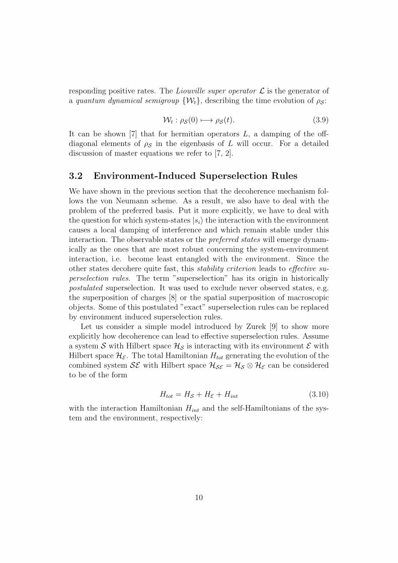
responding positive rates. The Liouville super operator L is the generator ofa quantum dynamical semigroup Wt, describing the time evolution of ρS :

Wt : ρS(0) 7−→ ρS(t). (3.9)

It can be shown [7] that for hermitian operators L, a damping of the off-diagonal elements of ρS in the eigenbasis of L will occur. For a detaileddiscussion of master equations we refer to [7, 2].

3.2 Environment-Induced Superselection Rules

We have shown in the previous section that the decoherence mechanism fol-lows the von Neumann scheme. As a result, we also have to deal with theproblem of the preferred basis. Put it more explicitly, we have to deal withthe question for which system-states |si〉 the interaction with the environmentcauses a local damping of interference and which remain stable under thisinteraction. The observable states or the preferred states will emerge dynam-ically as the ones that are most robust concerning the system-environmentinteraction, i.e. become least entangled with the environment. Since theother states decohere quite fast, this stability criterion leads to effective su-perselection rules. The term ”superselection” has its origin in historicallypostulated superselection. It was used to exclude never observed states, e.g.the superposition of charges [8] or the spatial superposition of macroscopicobjects. Some of this postulated ”exact” superselection rules can be replacedby environment induced superselection rules.

Let us consider a simple model introduced by Zurek [9] to show moreexplicitly how decoherence can lead to effective superselection rules. Assumea system S with Hilbert space HS is interacting with its environment E withHilbert space HE . The total Hamiltonian Htot generating the evolution of thecombined system SE with Hilbert space HSE = HS ⊗HE can be consideredto be of the form

Htot = HS +HE +Hint (3.10)

with the interaction Hamiltonian Hint and the self-Hamiltonians of the sys-tem and the environment, respectively:

10

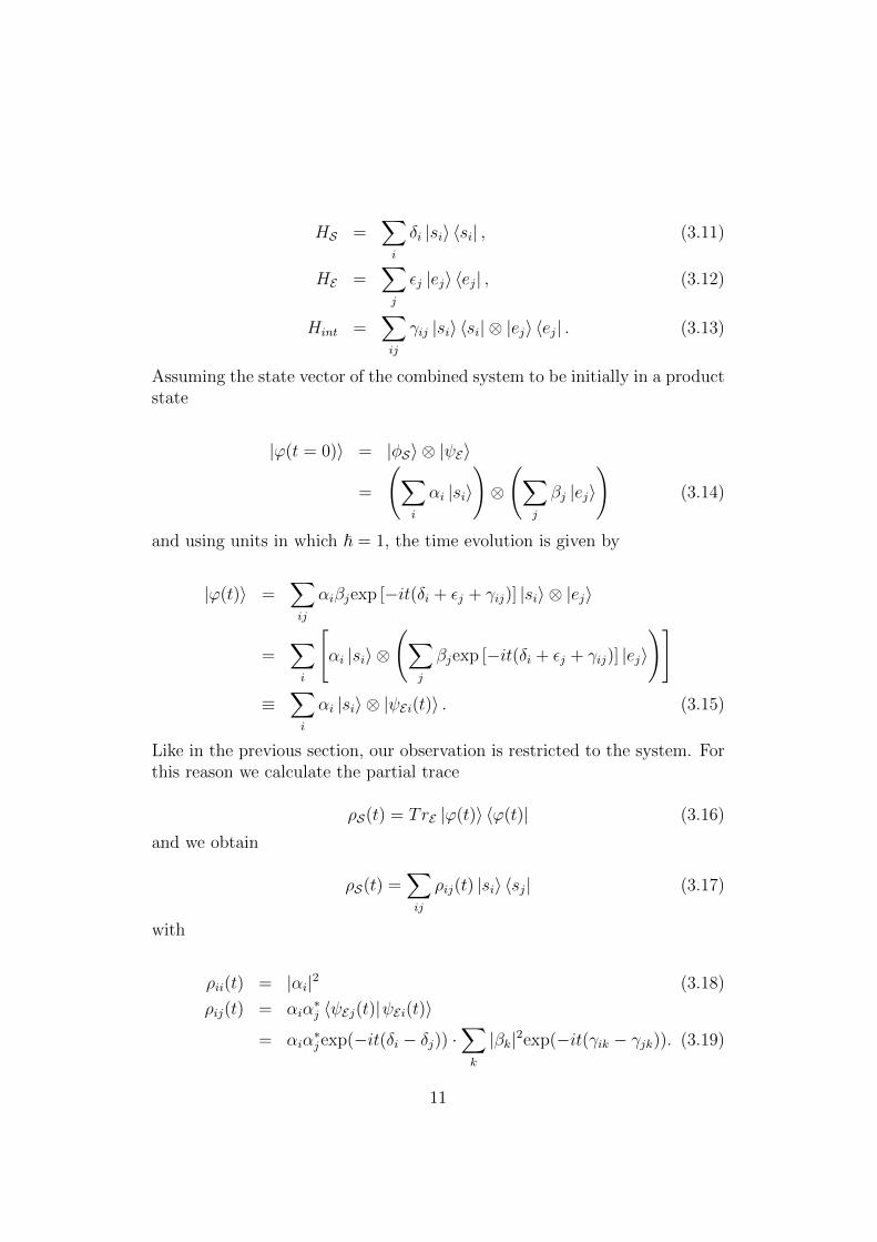
HS =∑i

δi |si〉 〈si| , (3.11)

HE =∑j

εj |ej〉 〈ej| , (3.12)

Hint =∑ij

γij |si〉 〈si| ⊗ |ej〉 〈ej| . (3.13)

Assuming the state vector of the combined system to be initially in a productstate

|ϕ(t = 0)〉 = |φS〉 ⊗ |ψE〉

=

(∑i

αi |si〉

)⊗

(∑j

βj |ej〉

)(3.14)

and using units in which ~ = 1, the time evolution is given by

|ϕ(t)〉 =∑ij

αiβjexp [−it(δi + εj + γij)] |si〉 ⊗ |ej〉

=∑i

[αi |si〉 ⊗

(∑j

βjexp [−it(δi + εj + γij)] |ej〉

)]≡

∑i

αi |si〉 ⊗ |ψEi(t)〉 . (3.15)

Like in the previous section, our observation is restricted to the system. Forthis reason we calculate the partial trace

ρS(t) = TrE |ϕ(t)〉 〈ϕ(t)| (3.16)

and we obtain

ρS(t) =∑ij

ρij(t) |si〉 〈sj| (3.17)

with

ρii(t) = |αi|2 (3.18)

ρij(t) = αiα∗j 〈ψEj(t)|ψEi(t)〉

= αiα∗jexp(−it(δi − δj)) ·

∑k

|βk|2exp(−it(γik − γjk)). (3.19)

11

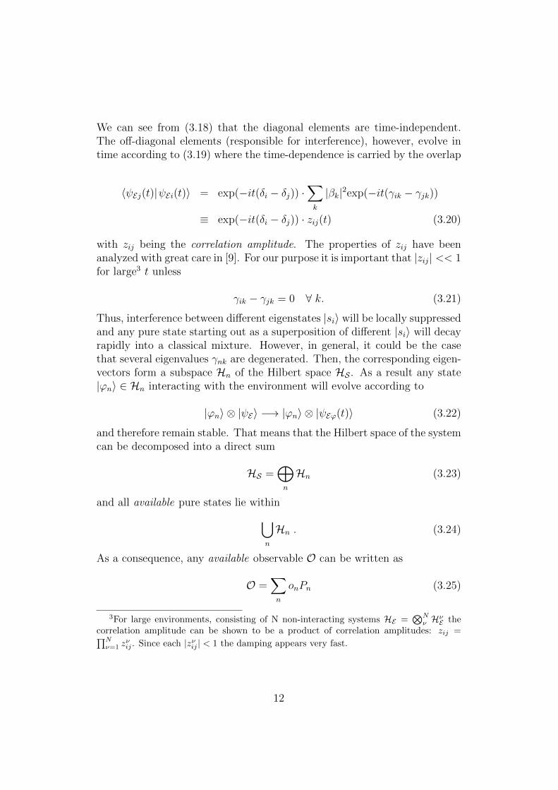
We can see from (3.18) that the diagonal elements are time-independent.The off-diagonal elements (responsible for interference), however, evolve intime according to (3.19) where the time-dependence is carried by the overlap

〈ψEj(t)|ψEi(t)〉 = exp(−it(δi − δj)) ·∑k

|βk|2exp(−it(γik − γjk))

≡ exp(−it(δi − δj)) · zij(t) (3.20)

with zij being the correlation amplitude. The properties of zij have beenanalyzed with great care in [9]. For our purpose it is important that |zij| << 1for large3 t unless

γik − γjk = 0 ∀ k. (3.21)

Thus, interference between different eigenstates |si〉 will be locally suppressedand any pure state starting out as a superposition of different |si〉 will decayrapidly into a classical mixture. However, in general, it could be the casethat several eigenvalues γnk are degenerated. Then, the corresponding eigen-vectors form a subspace Hn of the Hilbert space HS . As a result any state|ϕn〉 ∈ Hn interacting with the environment will evolve according to

|ϕn〉 ⊗ |ψE〉 −→ |ϕn〉 ⊗ |ψEϕ(t)〉 (3.22)

and therefore remain stable. That means that the Hilbert space of the systemcan be decomposed into a direct sum

HS =⊕n

Hn (3.23)

and all available pure states lie within⋃n

Hn . (3.24)

As a consequence, any available observable O can be written as

O =∑n

onPn (3.25)

3For large environments, consisting of N non-interacting systems HE =⊗N

ν HνE thecorrelation amplitude can be shown to be a product of correlation amplitudes: zij =∏Nν=1 z

νij . Since each |zνij | < 1 the damping appears very fast.

12

with Pn being the projection operators on the different subspaces Hn, re-spectively. This is equivalent to the statement that all available observableshave to fulfill

[O, Hint] = 0 (3.26)

which is sometimes called commutativity criterion.This model is an demonstrative example for how the interaction with the

environment superselects the most robust and therefore quasiclassical states.It can easily be extended to the case where a combined system-apparatus isinteracting with its environment in the following way:

|si〉 |ai〉 |E0〉 −→ |si〉 |ai〉 |Ei〉 ∀i (3.27)

In this case the interaction with the environment superselects the pointerstates and therefore implies the selection of the system states that can bemeasured by the apparatus[2, 9].

The model presented above makes use of a specific Hamiltonian. In gen-eral, however, we have to deal with an arbitrary total Hamiltonian, describingthe evolution of the system-environment state. Again, the stability crite-rion will lead to preferred system states. We can consider three differentcases of how the preferred states emerge through the interaction with theenvironment[2, 10]:

1. The quantum-measurement limit. In this case the evolution of the sys-tem is dominated by the interaction Hamiltonian Hint (Htot ≈ Hint).The model shown above falls into this category and it is therefore easyto see that the preferred system states will be the eigenstates of theinteraction Hamiltonian. In many cases, especially with macroscopicobjects, the interaction with the environment depends on force-lawswhich depend on the distance. Thus, leading to position eigenstates(see for example the scattering model of Joos and Zeh [7]).

2. The quantum limit of decoherence. This is the case when the evolutionof the system is dominated by the system’s self-Hamiltonian in the sensethat the highest energy available in the environment is smaller than theseparation between the system’s energy eigenstates - a situation oftenappearing in the microscopic regime. In this case the environmentcan only ”monitor” constants of motion, i.e., the energy. Thus, theinteraction with the environment, although it is weak in the abovesense, will lead to the energy eigenstates of HS being the preferredstates[10].

13

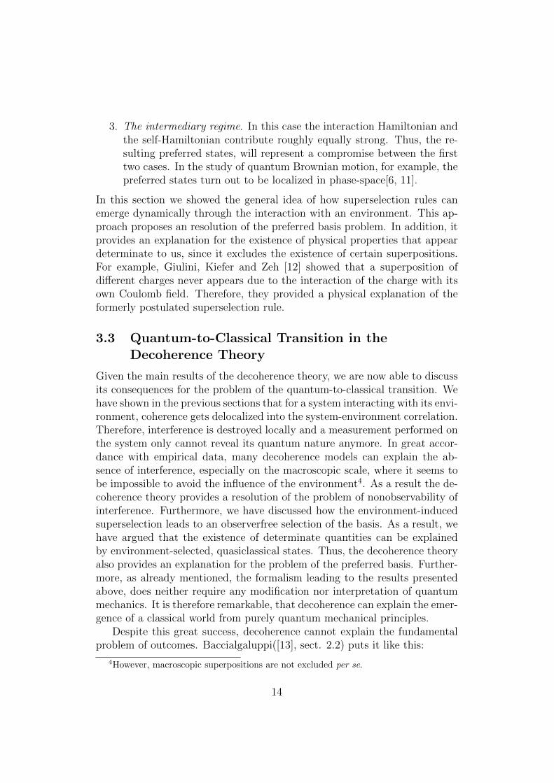
3. The intermediary regime. In this case the interaction Hamiltonian andthe self-Hamiltonian contribute roughly equally strong. Thus, the re-sulting preferred states, will represent a compromise between the firsttwo cases. In the study of quantum Brownian motion, for example, thepreferred states turn out to be localized in phase-space[6, 11].

In this section we showed the general idea of how superselection rules canemerge dynamically through the interaction with an environment. This ap-proach proposes an resolution of the preferred basis problem. In addition, itprovides an explanation for the existence of physical properties that appeardeterminate to us, since it excludes the existence of certain superpositions.For example, Giulini, Kiefer and Zeh [12] showed that a superposition ofdifferent charges never appears due to the interaction of the charge with itsown Coulomb field. Therefore, they provided a physical explanation of theformerly postulated superselection rule.

3.3 Quantum-to-Classical Transition in theDecoherence Theory

Given the main results of the decoherence theory, we are now able to discussits consequences for the problem of the quantum-to-classical transition. Wehave shown in the previous sections that for a system interacting with its envi-ronment, coherence gets delocalized into the system-environment correlation.Therefore, interference is destroyed locally and a measurement performed onthe system only cannot reveal its quantum nature anymore. In great accor-dance with empirical data, many decoherence models can explain the ab-sence of interference, especially on the macroscopic scale, where it seems tobe impossible to avoid the influence of the environment4. As a result the de-coherence theory provides a resolution of the problem of nonobservability ofinterference. Furthermore, we have discussed how the environment-inducedsuperselection leads to an observerfree selection of the basis. As a result, wehave argued that the existence of determinate quantities can be explainedby environment-selected, quasiclassical states. Thus, the decoherence theoryalso provides an explanation for the problem of the preferred basis. Further-more, as already mentioned, the formalism leading to the results presentedabove, does neither require any modification nor interpretation of quantummechanics. It is therefore remarkable, that decoherence can explain the emer-gence of a classical world from purely quantum mechanical principles.

Despite this great success, decoherence cannot explain the fundamentalproblem of outcomes. Baccialgaluppi([13], sect. 2.2) puts it like this:

4However, macroscopic superpositions are not excluded per se.

14

Intuitively, if the environment is carrying out, without our in-tervention, lots of approximate position measurements, then themeasurement problem ought to apply more widely, also to thesespontaneously occurring measurements.(...) The state of the ob-ject and the environment could be a superposition of zillions ofvery well localized terms, each with slightly different positions, andwhich are collectively spread over a macroscopic distance, even inthe case of everyday objects. (...) If everything is in interactionwith everything else, everything is entangled with everything else,and that is a worse problem than the entanglement of measuringapparatuses with the measured probes.

The superposition remains existent, at least globally, until some sort of ”col-lapse” has taken place. Therefore, the problem is shifted to the level of thetotal system-environment system and decoherence cannot provide any reso-lution. Any attempt to solve this problem requires an interpretation or anextension of standard quantum mechanics. We will discuss one of the latterapproaches in the next chapter.

Finally, we want to give an important remark. The entire concept ofdecoherence is based on a crucial assumption, namely that it is possible todivide the universe into subsystems. The state vector of the universe5 |ψ〉,evolves deterministically due to the Schrodinger equation. This poses no dif-ficulties, since our experience of classicality doesn’t apply to the observationof the entire universe from the outside. The problems arise from the divisioninto subsystems, which are the only subjects accessible for our observations.The universe is defined as a closed system. It is therefore, impossible to ap-ply the theory of decoherence to the entire universe. Thus, we cannot definequasiclassical properties for the universe itself by simply using the decoher-ence theory. One could therefore argue, that classicality is merely the resultof our subjective perception of only parts of the universe and the observedproperties are determined by the correlations between those parts. However,in general, there exists no criterion of how it is possible to divide the totalHilbert space into subspaces. As a conclusion, the crucial assumption, thatit is possible to divide the total Hilbert space into subspaces, is definitelynontrivial.

5If it is even possible to postulate such vector.

15

4 Collapse Theories

In this chapter we want to introduce another important approach to thequantum-to-classical transition. In contrast to the decoherence theory, Col-lapse theories not only deal with the problem of the preferred basis and theproblem of nonobservability of interference but also with the problem of out-comes. The basic idea is to modify the Schrodinger time evolution such thatan objective physical collapse can be achieved for each state vector. There-fore, the state vector obtains a ”realistic” status in collapse theories. The aimis to give a unified evolution for microscopic and macroscopic objects. Thus,the collapse process has to be very effective for macroscopic objects (such asmeasurement devices) on the one hand and negligible for microscopic objectson the other hand. We will show, that this can be achieved by postulatinga fundamental stochastic process contributing to the time evolution of thestate vector. Thereby, we restrict our self to the most studied models, thespontaneous localization model (GRW) introduced by Ghirardi, Rimini andWeber[14] and the continuous spontaneous localization model (CSL) intro-duced by Pearle [15].

4.1 Spontaneous Localization

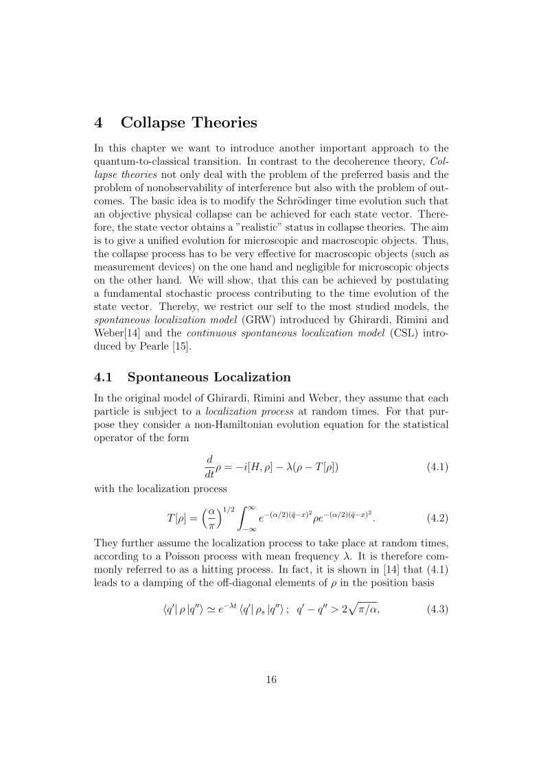
In the original model of Ghirardi, Rimini and Weber, they assume that eachparticle is subject to a localization process at random times. For that pur-pose they consider a non-Hamiltonian evolution equation for the statisticaloperator of the form

d

dtρ = −i[H, ρ]− λ(ρ− T [ρ]) (4.1)

with the localization process

T [ρ] =(απ

)1/2∫ ∞−∞

e−(α/2)(q−x)2ρe−(α/2)(q−x)2 . (4.2)

They further assume the localization process to take place at random times,according to a Poisson process with mean frequency λ. It is therefore com-monly referred to as a hitting process. In fact, it is shown in [14] that (4.1)leads to a damping of the off-diagonal elements of ρ in the position basis

〈q′| ρ |q′′〉 ' e−λt 〈q′| ρs |q′′〉 ; q′ − q′′ > 2√π/α, (4.3)

16

where we denote with ρs the pure Schrodinger evolution. It is further shownthat the diagonal elements evolve according to

〈q| ρ |q〉 ' 〈q| ρs |q〉 . (4.4)

Let us illustrate this by writing down the localization process according toBell [16] who reformulates the model to explicitly describe the effect on astate vector.

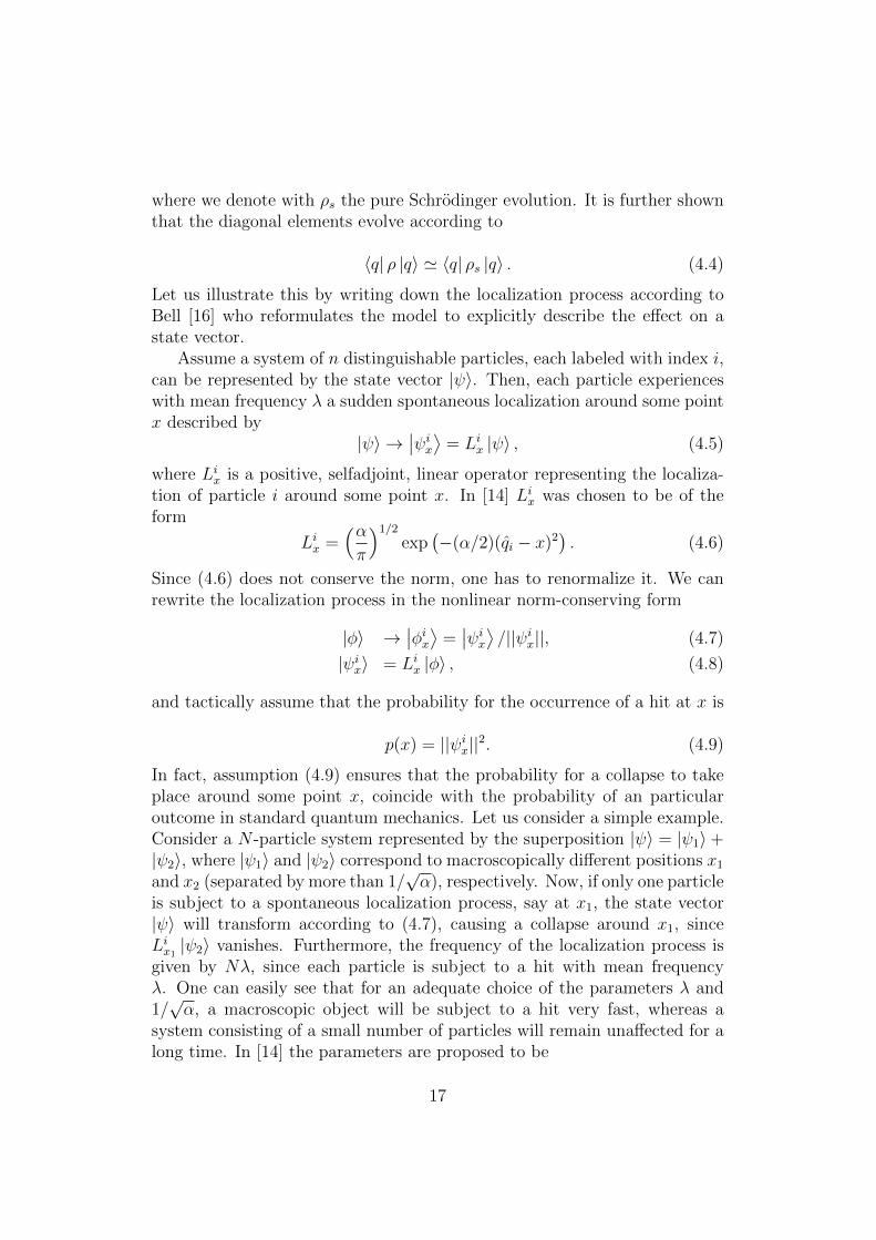
Assume a system of n distinguishable particles, each labeled with index i,can be represented by the state vector |ψ〉. Then, each particle experienceswith mean frequency λ a sudden spontaneous localization around some pointx described by

|ψ〉 →∣∣ψix⟩ = Lix |ψ〉 , (4.5)

where Lix is a positive, selfadjoint, linear operator representing the localiza-tion of particle i around some point x. In [14] Lix was chosen to be of theform

Lix =(απ

)1/2

exp(−(α/2)(qi − x)2

). (4.6)

Since (4.6) does not conserve the norm, one has to renormalize it. We canrewrite the localization process in the nonlinear norm-conserving form

|φ〉 →∣∣φix⟩ =

∣∣ψix⟩ /||ψix||, (4.7)

|ψix〉 = Lix |φ〉 , (4.8)

and tactically assume that the probability for the occurrence of a hit at x is

p(x) = ||ψix||2. (4.9)

In fact, assumption (4.9) ensures that the probability for a collapse to takeplace around some point x, coincide with the probability of an particularoutcome in standard quantum mechanics. Let us consider a simple example.Consider a N -particle system represented by the superposition |ψ〉 = |ψ1〉+|ψ2〉, where |ψ1〉 and |ψ2〉 correspond to macroscopically different positions x1

and x2 (separated by more than 1/√α), respectively. Now, if only one particle

is subject to a spontaneous localization process, say at x1, the state vector|ψ〉 will transform according to (4.7), causing a collapse around x1, sinceLix1 |ψ2〉 vanishes. Furthermore, the frequency of the localization process isgiven by Nλ, since each particle is subject to a hit with mean frequencyλ. One can easily see that for an adequate choice of the parameters λ and1/√α, a macroscopic object will be subject to a hit very fast, whereas a

system consisting of a small number of particles will remain unaffected for along time. In [14] the parameters are proposed to be

17

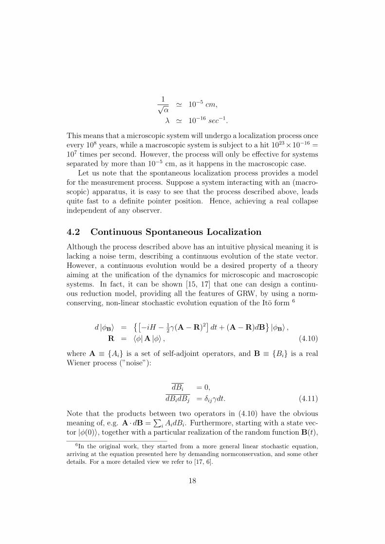
1√α' 10−5 cm,

λ ' 10−16 sec−1.

This means that a microscopic system will undergo a localization process onceevery 108 years, while a macroscopic system is subject to a hit 1023×10−16 =107 times per second. However, the process will only be effective for systemsseparated by more than 10−5 cm, as it happens in the macroscopic case.

Let us note that the spontaneous localization process provides a modelfor the measurement process. Suppose a system interacting with an (macro-scopic) apparatus, it is easy to see that the process described above, leadsquite fast to a definite pointer position. Hence, achieving a real collapseindependent of any observer.

4.2 Continuous Spontaneous Localization

Although the process described above has an intuitive physical meaning it islacking a noise term, describing a continuous evolution of the state vector.However, a continuous evolution would be a desired property of a theoryaiming at the unification of the dynamics for microscopic and macroscopicsystems. In fact, it can be shown [15, 17] that one can design a continu-ous reduction model, providing all the features of GRW, by using a norm-conserving, non-linear stochastic evolution equation of the Ito form 6

d |φB〉 =[−iH − 1

2γ(A−R)2

]dt+ (A−R)dB

|φB〉 ,

R = 〈φ|A |φ〉 , (4.10)

where A ≡ Ai is a set of self-adjoint operators, and B ≡ Bi is a realWiener process (”noise”):

dBi = 0,

dBidBj = δijγdt. (4.11)

Note that the products between two operators in (4.10) have the obviousmeaning of, e.g. A ·dB =

∑iAidBi. Furthermore, starting with a state vec-

tor |φ(0)〉, together with a particular realization of the random function B(t),

6In the original work, they started from a more general linear stochastic equation,arriving at the equation presented here by demanding normconservation, and some otherdetails. For a more detailed view we refer to [17, 6].

18

(4.10) gives rise to a certain state |φB(t)〉. Therefore, (4.10) generates an en-semble of state vectors. Given a set of commuting operators Ai, following[17], we will show that each |φB(t)〉 will converge towards an eigenvector ofthe operators A, corresponding to a reduction of |φ(0)〉 onto the commoneigenspaces of the operators A.

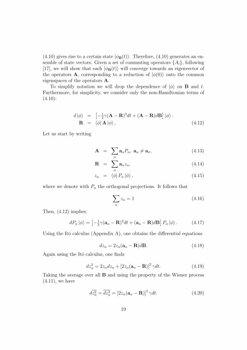
To simplify notation we will drop the dependence of |φ〉 on B and t.Furthermore, for simplicity, we consider only the non-Hamiltonian terms of(4.10):

d |φ〉 =[−1

2γ(A−R)2dt+ (A−R)dB

]|φ〉 .

R = 〈φ|A |φ〉 , (4.12)

Let us start by writing

A =∑α

aαPα, aα 6= aσ, (4.13)

R =∑α

aαzα, (4.14)

zα = 〈φ|Pα |φ〉 , (4.15)

where we denote with Pα the orthogonal projections. It follows that∑α

zα = 1 (4.16)

Then, (4.12) implies:

dPα |φ〉 =[−1

2γ(aα −R)2dt+ (aα −R)dB

]Pα |φ〉 . (4.17)

Using the Ito calculus (Appendix A), one obtains the differential equations

dzα = 2zα(aα −R)dB. (4.18)

Again using the Ito calculus, one finds

dz2α = 2zαdzα + [2zα(aα −R)]2 γdt. (4.19)

Taking the average over all B and using the property of the Wiener process(4.11), we have

dz2α = dz2

α = [2zα(aα −R)]2 γdt. (4.20)

19

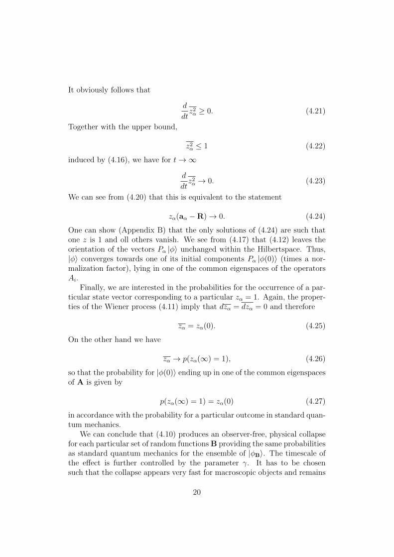
It obviously follows that

d

dtz2α ≥ 0. (4.21)

Together with the upper bound,

z2α ≤ 1 (4.22)

induced by (4.16), we have for t→∞

d

dtz2α → 0. (4.23)

We can see from (4.20) that this is equivalent to the statement

zα(aα −R)→ 0. (4.24)

One can show (Appendix B) that the only solutions of (4.24) are such thatone z is 1 and oll others vanish. We see from (4.17) that (4.12) leaves theorientation of the vectors Pα |φ〉 unchanged within the Hilbertspace. Thus,|φ〉 converges towards one of its initial components Pα |φ(0)〉 (times a nor-malization factor), lying in one of the common eigenspaces of the operatorsAi.

Finally, we are interested in the probabilities for the occurrence of a par-ticular state vector corresponding to a particular zα = 1. Again, the proper-ties of the Wiener process (4.11) imply that dzα = dzα = 0 and therefore

zα = zα(0). (4.25)

On the other hand we have

zα → p(zα(∞) = 1), (4.26)

so that the probability for |φ(0)〉 ending up in one of the common eigenspacesof A is given by

p(zα(∞) = 1) = zα(0) (4.27)

in accordance with the probability for a particular outcome in standard quan-tum mechanics.

We can conclude that (4.10) produces an observer-free, physical collapsefor each particular set of random functions B providing the same probabilitiesas standard quantum mechanics for the ensemble of |φB〉. The timescale ofthe effect is further controlled by the parameter γ. It has to be chosensuch that the collapse appears very fast for macroscopic objects and remains

20

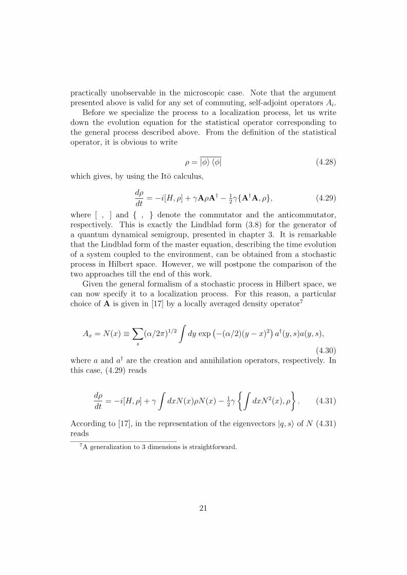
practically unobservable in the microscopic case. Note that the argumentpresented above is valid for any set of commuting, self-adjoint operators Ai.

Before we specialize the process to a localization process, let us writedown the evolution equation for the statistical operator corresponding tothe general process described above. From the definition of the statisticaloperator, it is obvious to write

ρ = |φ〉 〈φ| (4.28)

which gives, by using the Ito calculus,

dρ

dt= −i[H, ρ] + γAρA† − 1

2γA†A, ρ, (4.29)

where [ , ] and , denote the commutator and the anticommutator,respectively. This is exactly the Lindblad form (3.8) for the generator ofa quantum dynamical semigroup, presented in chapter 3. It is remarkablethat the Lindblad form of the master equation, describing the time evolutionof a system coupled to the environment, can be obtained from a stochasticprocess in Hilbert space. However, we will postpone the comparison of thetwo approaches till the end of this work.

Given the general formalism of a stochastic process in Hilbert space, wecan now specify it to a localization process. For this reason, a particularchoice of A is given in [17] by a locally averaged density operator7

Ax = N(x) ≡∑s

(α/2π)1/2

∫dy exp

(−(α/2)(y − x)2

)a†(y, s)a(y, s),

(4.30)where a and a† are the creation and annihilation operators, respectively. Inthis case, (4.29) reads

dρ

dt= −i[H, ρ] + γ

∫dxN(x)ρN(x)− 1

2γ

∫dxN2(x), ρ

. (4.31)

According to [17], in the representation of the eigenvectors |q, s〉 of N (4.31)reads

7A generalization to 3 dimensions is straightforward.

21

d

dt〈q′, s′| ρ |q′′, s′′〉 = − i 〈q′, s′| [H, ρ] |q′′, s′′〉

+ γ∑i,j

[G(q′i − q′′j )− 12G(q′i − q′j)

− 12G(q′′i − q′′j )]× 〈q′, s′| ρ |q′′, s′′〉 , (4.32)

whereG(q′i − q′′j ) = exp

(−1

4α(q′i − q′′j )2

)(4.33)

and the indices i and j label the particles. Then (4.32) describes the local-ization process for systems of particles separated by more than 1/

√α.

Let us follow an easy example presented in [18] to illustrate how thelocalization mechanism works. For this reason, we will concentrate on thecollapse dynamics alone and set H = 0 in (4.32). Now, consider a systemof particles in a superposition a |1〉 + b |2〉, where |1〉 and |2〉 describe Nparticles localized around some region 1 and some region 2, respectively.Further assume that region 1 and region 2 are separated by much more than1/√α. It is easy to see that (4.32) then yields

d

dt〈1| ρ |2〉 = γ

∑i,j

(0− 1

2· 1− 1

2· 1)× 〈1| ρ |2〉

= −γN2 〈1| ρ |2〉 , (4.34)

corresponding to a decay of the off-diagonal elements of ρ at the rate γN2.A similar result was obtained in the GRW model. In fact, it is shown in [17]that the hitting process of the GRW model and the continuous process of theCSL model are equivalent, taking the infinite frequency limit of the GRWprocess

λ→∞, α→ 0, 12λα = γ. (4.35)

4.3 Quantum-to-Classical Transition in the CollapseTheory

Based on the short introduction into spontaneous localization models givenabove, we are now able to discuss their consequences for the quantum-to-classical transition. We have seen in the previous section that adding astochastic term to the Schrodinger equation leads to a real physical col-lapse. In both, the GRW model as well as in the CSL model, an initial

22

superposed state turns into a statistical mixture of its constituents. The un-derlying mechanism is acting universally on every state vector, independentof any interaction with any other systems. Motivated by our experiencesin the everyday world, the process is chosen to take place in the positionbasis. However, we have shown in the previous section, that in principlethe mechanism works in an arbitrary basis, depending on the choice of theself-adjoint, commuting operators. Furthermore, for an adequate choice ofthe model’s parameters, the collapse mechanism is very effective for macro-scopic objects, whereas it leaves the Schrodinger evolution unchanged in themicroscopic case. Thus, providing an unified description for the occurrenceof superpositions in the microscopic regime and the absence of the latter onthe macroscopic scale. The true merit of the theory lies in the fact, thatit provides a resolution for the problem of outcomes. Since each individualstate vector is subject to a reduction process, the collapse model itself pro-vides a description of the measurement process, leading to real outcomes.The reduction postulate gets replaced by a physical reduction mechanism.

Despite this success, there are some remaining questions. The wholetheory is based on a modification of the Schrodinger equation. However, thismodification is postulated (e.g. the ”noise” field in the CSL model) and islacking a physical motivation. Furthermore, the reduction process is neverfully completed for a finite time. This is sometimes called the tails problem,which will become problematic if one wants to ascribe some kind of ”reality”to the reduced state, which is aspired in physical collapse theories.

Finally, we want to give an important remark. The modification of theSchrodinger equation should in principle produce some predictions, differentfrom them made by standard quantum mechanics. Thus, physical collapsetheories have to be seen as rival theories. We will discuss this in more detailin the last chapter.

5 Macroscopic Realism and Coarse-Grained

Measurements

Beside decoherence and the collapse theories, presented in the previous chap-ters, there exists another interesting approach concerning the quantum toclassical transition. In a recent work of Brukner and Kofler [24], it is arguedthat classicality arises from the restriction to coarse-grained measurements,i.e. the imprecision of a real measurement apparatus. Before we will showhow this can work, we have to introduce the notion of macroscopic realism(macrorealism) first defined by Leggett [22]. The idea is to explicitly write

23

down what we demand from a theory describing the macroscopic classicalworld we observe in our every-day life.

5.1 Legget-Garg Inequality

Macrorealism can be defined by the conjunction of the following threepostulates[19]:

(1) Macrorealism per se. A macroscopic object which has available to it twoor more macroscopically distinct states is at any given time8 in a definiteone of those states.

(2) Non-invasive measurability. It is possible in principle to determine whichof these states the system is in without any effect on the state itself oron the subsequent system dynamics.

(3) Induction The properties of ensembles are determined exclusively by ini-tial conditions (and in particular not by final conditions).

It is quite obvious that classical physics belongs to this class of macrorealistictheories.

Starting from these assumptions one can derive an inequality quite similarto the inequality introduced by Bell [20] or the Clauser-Horne-Shimony-Holt(CHSH) inequality [21]. Consider a macroscopic system and a correspondingquantity A, which whenever measured takes the values ±1. Further considera series of measurements performed on the system starting from identicalinitial conditions. In the first measurement A is measured at time t1 andt2, at t2 and t3 on the second, at t3 and t4 on the third and at t1 and t4on the fourth. Let us further denote with Ai the corresponding values of aparticular outcome at time ti. Similar to the CHSH case one can write:

A1(A2 − A4) + A3(A2 + A4) = ±2 (5.1)

Macrorealism per se is reflected by the existence of definite values of Ai at alltimes, and non-invasive measurability combined with induction is reflectedby the fact that the Ai’s are independent of the combination in which theyoccur. Given a series of such measurements, we can introduce temporalcorrelation functions

Cij = AiAj (5.2)

8Except for small transit times

24

Taking the average over (5.1) it follows that any theory based on the assump-tions of macrorealism has to satisfy the Leggett-Garg inequality [22]

K ≡ C12 + C23 + C34 − C14 ≤ 2. (5.3)

This equality can be used to test whether or not a system’s time evolutioncan be understood classical. Since standard quantum mechanics makes no apriori difference between microscopic and macroscopic systems, an isolatedquantum system violates the Leggett-Garg inequality (5.3). In fact, it can beexplicitly shown [23] that every non-trivial Hamiltonian leads to a violationof the inequality. However, in many cases (although not in all) decoher-ence (or physical collapse) is sufficient to restore macrorealism, since it turnssuperpositions into classical mixtures.

5.2 Coarse-Grained Measurement

Equipped with the definition of macrorealism, let us now illustrate the idea ofcoarse-grained measurement. Following [24], we will use a single spin coher-ent state. Spin-j coherent states are the eigenstates with maximal eigenvaluej of a spin operator pointing in the Ω ≡ (ϑ, ϕ) direction:

Jϑ,ϕ |Ω〉 = j |Ω〉 (5.4)

Further consider the Hamiltonian

H =J2

2I+ ωJx, (5.5)

where J is the rotor’s total spin vector operator, I the moment of inertia andω the angular precision frequency. Since J2 commutes with the individualspin components the time evolution operator can be written:

Ut ≡ e−iωtJx . (5.6)

Given a general spin coherent state, its representation in terms of Jz eigen-states |m〉, with corresponding possible eigenvalues m = −j,−j + 1, ..., j, isgiven by:

|Ωt〉 =∑m

(2jj+m

)1/2cosj+m(ϑt

2) sinj−m(ϑt

2)e−imϕt |m〉 . (5.7)

The probability of finding the particular outcome m in a Jz measurement attime t is given by the binomial distribution (Appendix C):

p(m, t) = | 〈m|Ωt〉 |2. (5.8)

25

In the macroscopic limit9, i.e. j 1, (5.8) can be written as a Gaussiandistribution

p(m, t) ≈ 1√2πσ

e−(m−µ)2

2σ2 , (5.9)

with standard deviation σ ≡√j/2 sin(ϑt) and mean value µ ≡ jcos (ϑt).

Now assume that the resolution of the measurement apparatus is restricted to∆m (which is a reasonable assumption in every realistic experiment). Thus,the 2j + 1 possible outcomes become reduced to 2j+1

∆m”slots” m of size ∆m.

In the case where the slot size is much larger than the standard derivation 10

∆m σ ∼√j (5.10)

the Gaussian (5.9) can not be distinguished from the discrete Kronecker delta

∆m√j : p(m, t)→ δm,µ (5.11)

where m is numbering the slots and µ number of the slot where the Gaussianis centered. If in addition j → ∞ (classical limit), the Kronecker delta willbecome the Dirac delta function

p(m, t)→ δ(m− µ). (5.12)

As a result, it is obvious that the action of a coarse grained measurement,represented by a projection operator

Pm ≡∑

m∈m

|m〉 〈m| , (5.13)

can be written as

Pm |Ω〉 ≈

|Ω〉 for µ inside m

0 for µ outside m.(5.14)

We can conclude that under the restriction of coarse-grained measurementwe are not able to resolve the superposition anymore and a the state seemsto have a definite value (the value assigned to the slot in which µ lies) fora Jz measurement at any time. This is macrorealism per se. Furthermore,

9The term ”macroscopic” used in [24] belongs to a system with a high dimensionalityrather than to a low-dimensional system with large parameters like mass or size.

10This is reasonable for large j since the countable number of distinguishable outcomesis limited by the apparatus 2j+1

∆m ≤ constant and j grows faster than√j

26

(5.14) shows that a measurement can be seen in good approximation as non-invasive(together with induction). Hence, no violation of the Leggett-Garginequality is possible anymore.

It is shown in [24] that the argumentation given above even holds foran arbitrary spin-j quantum state represented by a density matrix in theovercomplete basis of the coherent states

ρ =

∫ ∫f(Ω) |Ω〉 〈Ω| d2Ω (5.15)

where f(Ω) is a quasi-probability distribution with∫ ∫

f(Ω)d2Ω = 1.The argumentation given above uses an explicit Hamiltonian (5.5). In

the general case, it is shown in [23] that under the restriction of coarse-grained measurements an arbitrary spin-j quantum state can be describedby a classical mixture at any time. Thus, establishing macrorealism perse. However, non-invasive measurability follows not automatically. In [23] asufficient condition for macrorealism is given:

PmUt |Ω〉 ≈

Ut |Ω〉 for one m

0 for all the others.(5.16)

Therefore, the time evolution operator must produce superpositions of macro-scopically distinct states (states belonging to different slots) to violate macro-realism. However, Brukner and Kofler argue that Hamiltonians leading to aviolation of macrorealism are unlikely to appear in nature, due to their highcomplexity [23].

Let us emphasize that the approach of coarse-grained measurement re-lies only on standard quantum mechanics and the (reasonable) assumptionof insufficient precision of our measurement apparatuses. Furthermore, itis not at variance with the decoherence program, it only differs conceptu-ally. However, the formalism presented above deals with spin systems only.A generalization to other systems has not been done yet but would be aninteresting task.

6 Conclusion

We have seen various approaches to the question of the quantum-to-classicaltransition. We now want to summarize what they can offer to answer thisquestion and point out what they have in common or where they differ.

Let us start with the most commonly used approach, the decoherence pro-gram. We have seen that the interaction with an uncontrollable environment

27

not only explains quite well, why we do not see superpositions of macroscopicobjects, but also shows that the interaction even selects a preferred (pointer)basis. However, macroscopic superpositions are not per se excluded, sinceone could always (at least in principle) reduce the environment’s influence.Several experiments, e.g. interference of large molecules, have shown thatwe are able to control the environment better and better, maybe arriving ata point where we are faced with a real cat paradox. In addition, the deco-herence program is inherently quantum mechanical and therefore not ableto resolve the problem of outcomes. A further interpretation is needed toexplain why measurements have definite outcomes.

Now what can the collapse theories, presented in this work, tell us aboutthe quantum-to-classical transition? Although they are based on the modi-fication of the Schrodinger equation, they lead to predictions similar to de-coherence. This is not surprising, since in both cases a macroscopic super-position evoles into a classical mixture. In fact, the time evolution of asystem in both the decoherence and collapse theory can be described by amasterequation of the Lindblad form. However, the two approaches differon a fundamental level. In the case of the decoherence program, coherencebecomes destroyed only locally (and is still existing in the larger system-environment), whereas the collapse theory achieves a ”real” loss of coherenceon a fundamental level, i.e. independent of any interaction with some envi-ronment. Contrary to the decoherence program, the real physical collapseof each state vector explains why we have definite outcomes in every mea-surement. Furthermore, the collapse theory provides a real boarder for theobservability of superpositions, i.e. superpositions are a priori excluded atsome level. However, the mechanism provided by the collapse theories suffersfrom the preferred basis problem. This means that the choice of the operatorin the additional term of the Schrodinger equation determines in which basisthe collapse can be achieved. This seems to be unsatisfying. Furthermorethe modification lacks a physical motivation in general.

Anyhow, we want to emphasize that it is not a matter of taste, whichapproach one prefers. We point out again that, due to the modification ofthe Schrodinger equation, the collapse theory is a real rival theory, concerningstandard quantum mechanics. However, since decoherence effects are foundto be much stronger in the present experimental setups, it is still impossible totest collapse models against quantum theory. Hopefully, future experiments,e.g. with huge molecules, will become sensitive enough, to confirm or excludecollapse theories.

Since the approach of coarse-grained measurements only differs conceptu-ally from decoherence on the one hand, and is still demanding a generalizationon the other hand, we do not want to say much about it. However, in the

28

authors view it is an interesting idea. Especially due to the fact that therealistic assumption of imprecise measurement apparatuses can lead to theemergence of classicality.

Finally, we have seen that there exist a lot of explanations for the ap-pearance of a classical world in quantum theory. However, there still existan important issue which we have not talked about. Even if it was possibleto explain the nonobservability of macroscopic superpositions, to answer thequestion of the quantum-to-classical transition we still would have to explainexplicitly the emergence of classical physics, i.e. to show that it is possibleto derive Newton’s laws from quantum theory.

29

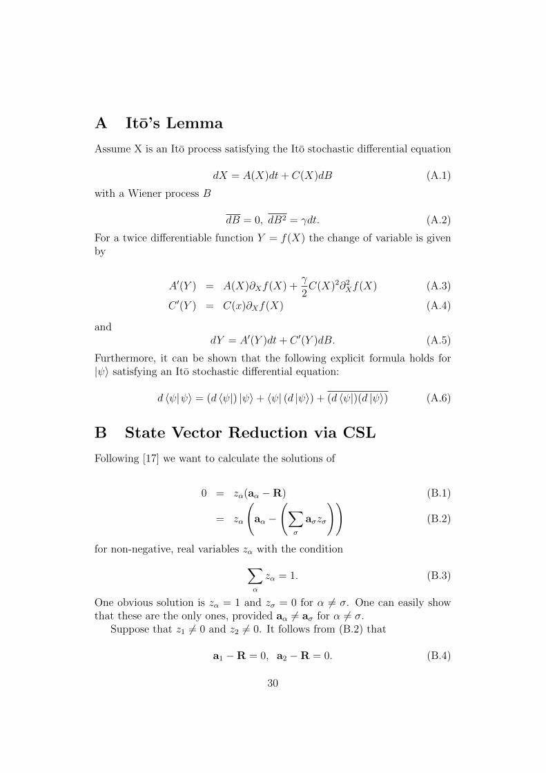
A Ito’s Lemma

Assume X is an Ito process satisfying the Ito stochastic differential equation

dX = A(X)dt+ C(X)dB (A.1)

with a Wiener process B

dB = 0, dB2 = γdt. (A.2)

For a twice differentiable function Y = f(X) the change of variable is givenby

A′(Y ) = A(X)∂Xf(X) +γ

2C(X)2∂2

Xf(X) (A.3)

C ′(Y ) = C(x)∂Xf(X) (A.4)

anddY = A′(Y )dt+ C ′(Y )dB. (A.5)

Furthermore, it can be shown that the following explicit formula holds for|ψ〉 satisfying an Ito stochastic differential equation:

d 〈ψ|ψ〉 = (d 〈ψ|) |ψ〉+ 〈ψ| (d |ψ〉) + (d 〈ψ|)(d |ψ〉) (A.6)

B State Vector Reduction via CSL

Following [17] we want to calculate the solutions of

0 = zα(aα −R) (B.1)

= zα

(aα −

(∑σ

aσzσ

))(B.2)

for non-negative, real variables zα with the condition∑α

zα = 1. (B.3)

One obvious solution is zα = 1 and zσ = 0 for α 6= σ. One can easily showthat these are the only ones, provided aα 6= aσ for α 6= σ.

Suppose that z1 6= 0 and z2 6= 0. It follows from (B.2) that

a1 −R = 0, a2 −R = 0. (B.4)

30

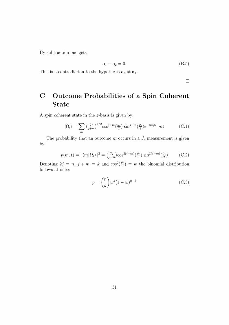
By subtraction one gets

a1 − a2 = 0. (B.5)

This is a contradiction to the hypothesis aα 6= aσ.

C Outcome Probabilities of a Spin Coherent

State

A spin coherent state in the z-basis is given by:

|Ωt〉 =∑m

(2jj+m

)1/2cosj+m(ϑt

2) sinj−m(ϑt

2)e−imϕt |m〉 (C.1)

The probability that an outcome m occurs in a Jz measurement is givenby:

p(m, t) = | 〈m|Ωt〉 |2 =(

2jj+m

)cos2(j+m)(ϑt

2) sin2(j−m)(ϑt

2) (C.2)

Denoting 2j ≡ n, j + m ≡ k and cos2(ϑt2

) ≡ w the binomial distributionfollows at once:

p =

(n

k

)wk(1− w)n−k (C.3)

31

References

[1] E. Schrodinger. Die gegenwartige Situation in der Quantenmechanik.Naturwissenschaften, 23(49):823–828, 1935.

[2] Maximilian Schlosshauer. Decoherence and the Quantum-to-ClassicalTransition. Springer, 2007.

[3] J. von Neumann. Mathematische Grundlagen der Quantenmechanik.Springer, 1932.

[4] E. Schmidt. Zur Theorie der linearen und nichtlinearen Integralgleichun-gen. Math. Annalen, 63:433–476, 1907.

[5] A. Einstein, B. Podolsky, and N. Rosen. Can Quantum-MechanicalDescription of Physical Reality Be Considered Complete? Phys. Rev.,47:777–780, May 1935.

[6] E. Joos, H.D. Zeh, C. Kiefer, D.Giulini, J.Kupsch and I.-O. Stamatescu.Decoherence and the Appearance of a Classical World in Quantum The-ory. Springer, 2003.

[7] E. Joos and H.D. Zeh. The emergence of classical properties throughinteraction with the environment. Zeitschrift fur Physik B CondensedMatter, 59(2):223–243, 1985.

[8] G. C. Wick, A. S. Wightman, and E. P. Wigner. Superselection Rulefor Charge. Phys. Rev. D, 1:3267–3269, Jun 1970.

[9] W. H. Zurek. Environment-Induced Superselection Rules. Phys. Rev.D, 26:1862–1880, Oct 1982.

[10] J.P. Paz and W. H. Zurek. Quantum Limit of Decoherence: Environ-ment Induced Superselection of Energy Eigenstates. Phys. Rev. Lett.,82:5181–5185, Jun 1999.

[11] W. H. Zurek, S. Habib, and J.P. Paz. Coherent States via Decoherence.Phys. Rev. Lett., 70:1187–1190, Mar 1993.

[12] D. Giulini, C. Kiefer, and H.D. Zeh. Symmetries, superselection rules,and decoherence. Physics Letters A, 199(56):291 – 298, 1995.

[13] Guido Bacciagaluppi. The role of decoherence in quantum mechanics.In Edward N. Zalta, editor, The Stanford Encyclopedia of Philosophy.Winter 2012 edition, 2012.

32

[14] G. C. Ghirardi, A. Rimini, and T. Weber. Unified dynamics for micro-scopic and macroscopic systems. Phys. Rev. D, 34:470–491, Jul 1986.

[15] P. Pearle. Combining stochastic dynamical state-vector reduction withspontaneous localization. Phys. Rev. A, 39:2277–2289, Mar 1989.

[16] J.S. Bell. in Schrodinger - Centenary Celebration of a Polymath. Cam-bridge University Press, 1987.

[17] G. C. Ghirardi, P. Pearle, and A. Rimini. Markov processes in Hilbertspace and continuous spontaneous localization of systems of identicalparticles. Phys. Rev. A, 42:78–89, Jul 1990.

[18] P. Pearle, J. Ring, Juan I. Collar, and Frank T. Avignone III. The CSLCollapse Model and Spontaneous Radiation: An Update. Foundationsof Physics, 29(3):465–480, 1999.

[19] A. J. Leggett. Testing the limits of quantum mechanics: motiva-tion, state of play, prospects. Journal of Physics: Condensed Matter,14(15):R415–R451, 2002.

[20] J.S. Bell. On the Einstein Podolsky Rosen paradox. Physics, 1(3):195–200, 1964.

[21] J. F. Clauser, M. A. Horne, A. Shimony, and R. A. Holt. ProposedExperiment to Test Local Hidden-Variable Theories. Phys. Rev. Lett.,23:880–884, Oct 1969.

[22] A. J. Leggett and A. Garg. Quantum mechanics versus macroscopicrealism: Is the flux there when nobody looks? Phys. Rev. Lett., 54:857–860, Mar 1985.

[23] J. Kofler and C. Brukner. Conditions for Quantum Violation of Macro-scopic Realism. Phys. Rev. Lett., 101:090403, Aug 2008.

[24] J. Kofler and C. Brukner. Classical World Arising out of QuantumPhysics under the Restriction of Coarse-Grained Measurements. Phys.Rev. Lett., 99:180403, Nov 2007.

33