The Anatomy of the Chua circuit Bachelor Thesis Equivalent to 15 ECTS

Jakob Lavröd

Supervisor: Sven Åberg

VT 2014

Division of Mathematical

Physics Department of Physics

Faculty of Science

Abstract

The Chua circuit, known to exhibit chaotic behaviour, has been constructed and studied. The goal was to investigatethe experimental underpinning of the theory. The component relationship of the resistors, capacitors, inductors andoperational amplifiers have been measured and established within their domain of validity.

The system equations themselves cannot be directly validated through a traditional simulation vs. experimentalstudy due to the chaotic property. Instead, a novel procedure is proposed where the system variables are split intogroups, with each group being validated by obtaining the variables outside the group directly from experimental data.The method decisively confirms the equations and parameters values to be correct.

To streamline the theoretical computations, the special piecewise linear structure of the system equations is usedto obtain local analytical solutions, which are then joined together by equation solving. Using the resistance as thecontrol parameter, the different solutions to the equations are classified and qualitatively explained. A number ofexperimental tests are performed to investigate the correspondence between theory and experiments; the invarianceunder parity inversion, the position of the Hopf bifurcation and the equilibrium voltage as a function of resistance.

Finally, chaos is quantified using the Lyapunov exponent. As its definition requires a metric, such is proposedbased on energy consideration. The piecewise linear structure of the equation provides a very simple formula for theLyaupnov exponent in terms of averaging over the Generalized Rayleigh quotient along a trajectory. The Lyaupnovexponent is evaluated as a function of resistance and compared with the qualitative conclusions about the circuit.

1

List of abbreviations

PWLDES . . . . . . . Piecewise linear differential equation solver

RK4 . . . . . . . . . . . . . Runge-Kutta method of fourth order

ODE45 . . . . . . . . . . In-built algorithm in Matlab to solve differential equations using the Runge-Fehlberg method.

ODE113 . . . . . . . . . In-built algorithm in Matlab using an adaptive Runge-Kutta method of order 13

ODE15 . . . . . . . . . . Implicit Runge-Kutta method in-built in Matlab

2

Contents

1 Introduction 4

2 Background of the Chua circuit 42.1 Derivation of the Chua circuit . . . . . . . . . . . . . . . . . . . . . . . . . . . . . . . . . . . . . . . . . . . 42.2 Review of previous research . . . . . . . . . . . . . . . . . . . . . . . . . . . . . . . . . . . . . . . . . . . . 6

3 Testing of the components 63.1 Resistors and Potentiometers . . . . . . . . . . . . . . . . . . . . . . . . . . . . . . . . . . . . . . . . . . . 63.2 Capacitors . . . . . . . . . . . . . . . . . . . . . . . . . . . . . . . . . . . . . . . . . . . . . . . . . . . . . . 73.3 Inductor . . . . . . . . . . . . . . . . . . . . . . . . . . . . . . . . . . . . . . . . . . . . . . . . . . . . . . . 83.4 Operational amplifier and the Chua diode . . . . . . . . . . . . . . . . . . . . . . . . . . . . . . . . . . . . 9

4 Derivation and solution of the system equations 114.1 Derivation of the Chua equations . . . . . . . . . . . . . . . . . . . . . . . . . . . . . . . . . . . . . . . . . 114.2 Method of numerical solutions for the equations . . . . . . . . . . . . . . . . . . . . . . . . . . . . . . . . . 11

5 Validation of the equations 135.1 Derivation of the validation method . . . . . . . . . . . . . . . . . . . . . . . . . . . . . . . . . . . . . . . 135.2 Application to theoretical and experimental datasets . . . . . . . . . . . . . . . . . . . . . . . . . . . . . . 15

6 Solutions of the equations 176.1 The equilibrium solution . . . . . . . . . . . . . . . . . . . . . . . . . . . . . . . . . . . . . . . . . . . . . . 186.2 The Hopf bifurcation . . . . . . . . . . . . . . . . . . . . . . . . . . . . . . . . . . . . . . . . . . . . . . . . 186.3 The single scroll attractor . . . . . . . . . . . . . . . . . . . . . . . . . . . . . . . . . . . . . . . . . . . . . 196.4 The double scroll attractor . . . . . . . . . . . . . . . . . . . . . . . . . . . . . . . . . . . . . . . . . . . . 216.5 The outmost limit cycle . . . . . . . . . . . . . . . . . . . . . . . . . . . . . . . . . . . . . . . . . . . . . . 22

7 Lyapunov exponents of the circuit 237.1 Measures of chaos . . . . . . . . . . . . . . . . . . . . . . . . . . . . . . . . . . . . . . . . . . . . . . . . . 237.2 Choice of metric . . . . . . . . . . . . . . . . . . . . . . . . . . . . . . . . . . . . . . . . . . . . . . . . . . 247.3 Computation of the Lyapunov exponents . . . . . . . . . . . . . . . . . . . . . . . . . . . . . . . . . . . . . 247.4 Lyapunov exponents for different resistances . . . . . . . . . . . . . . . . . . . . . . . . . . . . . . . . . . . 27

8 Conclusions and outlook 28

9 Self-reflections 28

10 Acknowledgments 29

3

1 Introduction

This thesis was inspired by the following 2014 International Young Physicists Tournament problem:

It is known that some electrical circuits exhibit chaotic behaviour. Build a simple circuit with such a property,and investigate its behaviour. [1]

The key word in this problem formulation is "chaotic". The ordinary usage of the word implies complete disorder [2] - acoin toss might seem like the perfect example as nobody can predict the outcome. However, from a scientific-deductiveperspective such a system is rather trivial as we can easily quantify the different outcomes as equaprobable and there isno possibility to produce more sofisticated predictions. We call these systems stochastic in contrast to predictable oneswhich are labeled determinstic.However, in 1890 Henri Poincaré indicated that systems could go from determinstic to stochastic as time progressed inthe sense that prediction would start out very precise, but would end up no better than a coin toss [3]. Hence the conceptof chaos is informally defined as the gradual loss of predicitability as time progresses. In 1961 Edward Lorentz providedan example of such a system in the form of a set of coupled differential equations describing an idealized model of theatmosphere [3].Some scientists questioned the physical nature of Lorentz’ result, by stating that the model introduced was so crude andsimplified that no real experimental confirmation could be made. They claimed that the phenomenon was so atypicalthat it could only be exhibited by abstract mathematical models with no connection to reality. In order to investigatethe phenomenon, the research group of Takashi Matsumoto started building an electrical circuit that would mimicthe equations [4]. Given that the multiplications that appear in the equations are rather complicated to implementelectronically, the circuit itself became horrendously complex.After several years of work, the circuit was finally completed in October of 1983 and was to be demonstrated to LeonChua, a visiting professor. However, the premiere was a spectacular disaster due to the failure of one of the integratedcircuits. Because of this nonsuccess, Chua wondered if one could not construct a much simpler circuit that would not begoverned by the Lorentz equations, but would still give rise to chaotic behaviour. As the hallmark of a true genius, Chuarealized exactly how he should remove all the unnecessary components of the circuit while still preserving the chaos. Thissimple device behaved just as Chua had predicted [5] and showed that chaotic behaviour is in no way restricted to theabstract world of mathematics, but can be easily constructed and observed. The Chua circuit was born.The ease of construction and observability of the Chua circuit makes the circuit a very natural candidate for the studyof chaos. Although one of the main motivations behind the circuit was to provide a physical realization of a set ofdifferential equations giving rise to chaos - there have been several hundred papers written on the topic[4] - rather littleattention has been given to experimentally verify the theoretical model Chua proposed beyond a visual comparisionbetween simulation and measurements [6]. The first goal of this thesis is therefore to try to rectify this by providingexperimental vindication of the theory, building from the component level up to the qualitative features where mostresearch is carried out. Secondly, most works on the Chua circuit relay heavily on the standard methods of chaos theoryand differential equations. However as will be seen in the equations that govern the circuit, there exists a piecewise linearstructure that can be exploited to speed up the computations significantly.The following work is divided into six main sections. Section 2 introduces the Chua circuit, and shows why it is oneof the most natural choices when studing a chaotic circuit. In section 3 the properties of the electrical components aremeasured. In section 4 the relevant equations a method of solution is derived. In section 5 the validity of the equationsare investigated. In section 6 the different kinds of solutions are investigated. In section 7 chaos is quantified using theLyapunov exponent. Finally, the ramification and future applications of the work is discussed in section 8.

2 Background of the Chua circuit

2.1 Derivation of the Chua circuit

"Chaotic" is often confused with the concept "complicated". A system of the latter type would consist of a large numberof components interacting in a very intricate way, and might very well be chaotic. However, if the only goal is to obtainchaotic behaviour, there is no inherent rule that forces us to make the circuit very complicated. Part of Chua’s geniuswas to realize that a simple circuit is enough to demonstrate chaos. By sticking with this thinking, we will try to derivein what sense the Chua circuit can be considered "the simplest chaotic circuit", as it is often called in the literature [7],since this makes it a natural candidate for an in-depth investigation of chaotic behaviour.The first watershed between different circuits is whether the system is autonomous or nonautonomous, meaning wheneverthe system is explicitly independent of time or not [8]. Such time dependence could arise from variation in the externalpower source or some system parameter. For simplicity one often wants to keep the system independent of the surround-ings as this simplifies the mathematical treatment and also has the nice feature that the resulting dynamic become anemergent property, not something externally created.

4

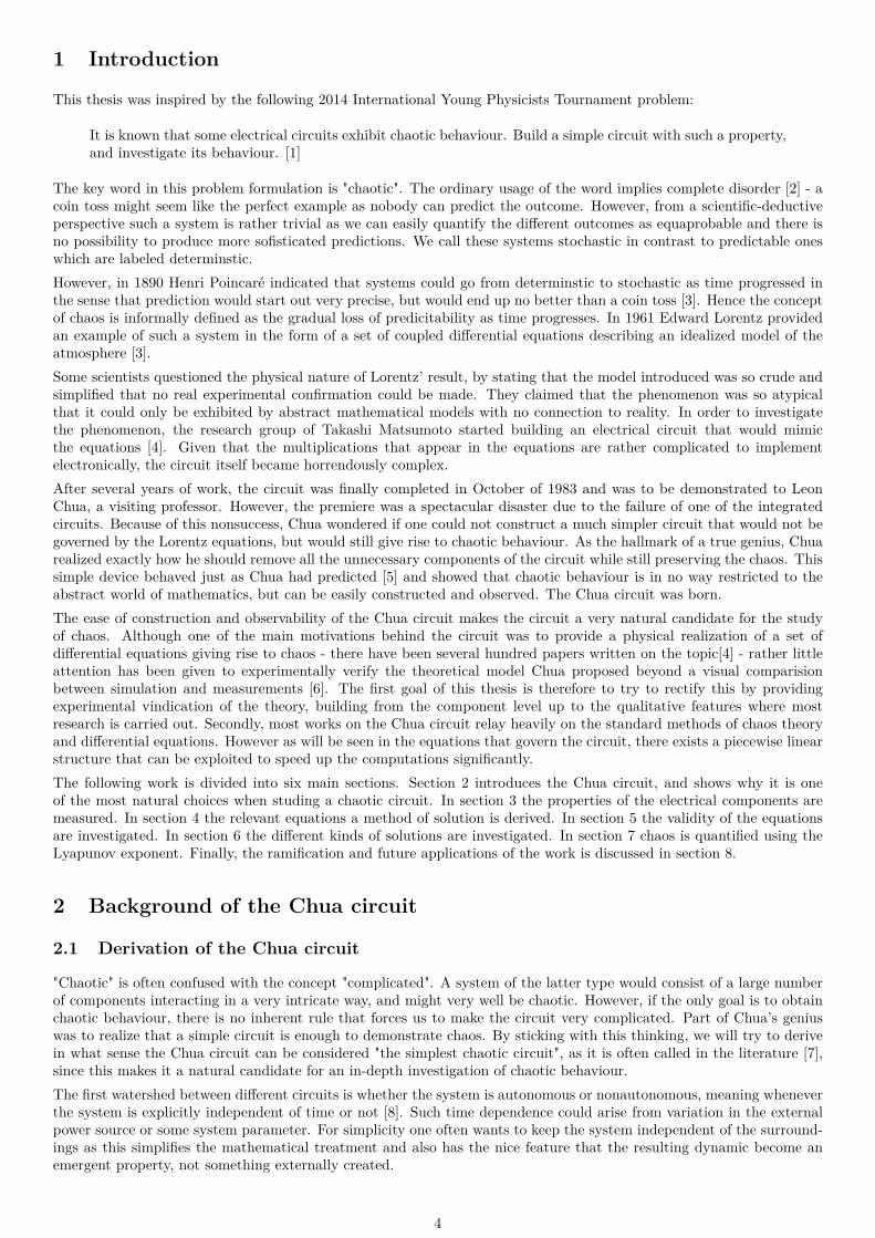
It was noted above that there is no need to make the circuit overly complicated to get chaos. On the other hand it is alsointuitively clear that one has to reach a certain minimal complexity. This is mathematically captured by the Poincaré-Bendixson theorem according to which a system must have at least three degrees of freedom to be able to exhibit chaoticbehaviour [8].The number of degrees of freedom is determined by the number of energy carrying components, as these describe howmany different states the system can be in.To understand this, note that the number of degrees of freedom describeshow many scalar quantities (at each moment in time) are needed to fully classify the state of the circuit, meaning thatevery voltage and current can be computed from such information. If the system contained only resistive componentsall currents and voltages could be computed directly, without any additional knowledge. Therefore, such system wouldhave zero degrees of freedom. What characterizes an energy carrying component is that the relation between voltageand current depends on the previous history (such as a differential relation). With only access to information of thecurrent moment, both of them cannot be inferred, instead one of them must be known, adding one degree of freedomper component. An easy way to look at the capacitor, for example is as a current source with the current depending onthe change in voltage. If the information about this current is provided, it can be treated just like an ordinary currentsource and the resulting resistive equations can be solved. In the same manner, an inductor can be treated as a voltagesource that has a voltage depending on the change in current. To build a minimal chaotic system, one should thereforeuse three components that can store energy.Linear systems cannot exhibit chaotic behaviour [9]. A simple way to understand this is to note that the behaviour of thelinear systems is independent of the scale, meaning that the dynamics happening for small values of the system variableswill still happen for larger values, there is simply speaking not any surprises that can ruin the predictability. Therefore onemust also include a non-linear component. The simplest possibility is to make this component purely resistive, excludingcomponents like iron core inductors with strong hysteresis or diodes with parasitic capacitance, as these devices have amemory that drastically complicates the resulting equations. This still leaves quite a lot of possibilities in the form oftransistors, varistors, diodes and many more, with several of these being used in actual chaotic circuits [10].Among the alternatives, one stands aside as maybe the simplest of them all: the operational amplifier [11], denoted bythe symbol shown figure 1. It is important to note that with simplicity we do not mean that of inner design (whichis rather complicated for the operational amplifier compared to many other devices) but that of device characteristics.This (ideal) component is simply a linear amplifier between the input voltage difference (between the plus and minusterminal) and the output node. The amplification is limited to the maximum supplied voltage, after which the outputvoltage is constant. The entire characteristics is shown in figure 2. A practical feature of the device is that it is locallyactive, meaning that it can supply the circuit with power due to its connection to a voltage source.

Figure 1: Operational ampli-fier symbol

Figure 2: Operational amplifier characteristics be-tween voltage difference and amplified voltage

The rather surprising fact first proven by Chua, known as the Global Unfolding Theorem, is that a circuit satisfying thesethree criteria (autonomous, three energy storing components and the only nonlinear devices are operational amplifiers)either contains more operational amplifiers than minimally needed for chaos or is conjugate to family of circuits of theChua-Kennedy form shown in figure 3 in the sense that for any other circuit outside of this family there exists a lineartransformation that transforms the equations back into the Chua-Kennedy set for some values of the physical constants[12]. Hence the Global Unfolding Theorem provides mathematical rigor to the statement that the Chua circuit is "thesimplest chaotic circuit" and motivate its use as a model system for chaotic systems.Figure 3 shows the component values that were chosen for the circuit used in this thesis. These values were selected tospan as many different behaviours as possible of the circuit. The design was implemented on a circuit board as can beseen in figure 4 and soldered together for maximal quality.

5

Figure 3: Circuit diagram of Chua circuit used in ex-periments Figure 4: Picture of Chua circuit used in experiments

2.2 Review of previous research

The research on the Chua circuit has been both broad and extensive. Only 10 years after the conception of the circuit,Chua himself estimated that more than 200 papers had been written [4]. We will make no attempt to fully review sucha massive amount of research. However, it is possible to identify three rather loose themes in the literature and we willuse these to provide context for our own study, most prominently the need for systematic investigation of the circuit’sanatomy.The first theme focuses on the properties of the circuit itself. Besides the first papers investigating the chaotic behaviournumerically [13] and experimentally [5], the most essential one contain a formal proof by Chua to show that the system istruly chaotic [14], putting the chaos theory of the Chua circuit on solid ground. Most of the research done on the circuithas focused on qualitative properties such as the bifurcation diagram, which depends on some control parameter [15],the different form of the attractors that can appear [16] or construction of discrete maps to explain different features ofthe solutions [17]. As all of these results presuppose that the underlying set of differential equations is correct, a positionoften taken for granted without any test of validity, preparing the ground for this thesis.The second theme focuses on alternative designs of the Chua circuit.In many early studies, such as the original papers from 1984-86, the resistance in series with the inductor is left out[13],[5]. Even if no such component is added physically to the circuit, in practice one can never get rid of the parasiticresistance in the inductor itself, a fact pointed out by [18]. As it is not needed to obtain chaos, attempts have been madeto minimize its size in order to simplify the circuit, but it has also been explicitly included in the theoretical model.Several studies also argue for replacing the physical coil with a simulated inductor built with resistors, capacitors andoperational amplifiers, known as a gyrator. The arguments for this change include obtaining lower frequency signals (sesuch issues below) [19], higher component quality [20], smaller non-linear effects and smaller size [21]. However, directexperimental comparison between a physical inductor and a simulated inductor is scarce in the literature; motivatingsuch an investigation.Additionally, quite a few alternative designs aim at changing the operational amplifiers. There are mainly two reasonsfor doing this: Either to increase the performance of the circuit under high frequency oscillations [22] or to be ableto investigate the behaviour of the circuit with a smoother non-linearity [23]. While the first point was experimentallycircumvented, in the second case there is a strong argument for restricting to the piecewise-linear case as previous researchshow that no new qualitative phenomena appear [24].The third theme, that includes a vast majority of the current research in the field, features the use of the Chua circuitin different applications. This accounts for everything from the synchronization of multiple circuits [25] applied to secretcommunication [26] to the control of chaos by including an extra voltage input source [27].The utility of the Chua circuit also exceedes that of its physical realization in the sense that it is seen as a model systemfor chaos [28]. Many algorithms aimed at investigating different features of chaotic systems, such as distinguishing chaosfrom random noise [29] or general attractor reconstruction [30] use data generated from a Chua circuit. It is crucial forsuch studies that the physical realization is accurately described by the theoretical model as this might otherwise causea discrepancy, not due to a faulty algorithm, but instead due to the inadequacy of the original model. One goal of thiswork has therefore also been to try to identify possible pitfalls that might cause such deviations.

3 Testing of the components

3.1 Resistors and Potentiometers

The resistor is the most basic of the electrical components used and rarely requires special attention. In order to havegood quality, metal film resistors were used, having low noise, weak nonlinearity and relative insensitivity to temperature

6

variations [31]. To verify the ideality of the resistor, the frequency response was measured (see the inductor section fordetails) showing no frequency dependence in the interval 0-200 kHz.To be able to obtain different qualitative behaviours of the circuit, a control parameter that can be varied is needed andthe resistor R was selected for this purpose, as most other components are not only hard to change systematically, butalso to measure precisely. Variation of the paramter was achieved by three potentionmeters (2000 Ω, 500 Ω, 20 Ω) inseries in order to get different degrees of fine-tuning.There is also a need to have very precise measurements of the resistance as the qualitative behaviour of the systemis very strongly dependent upon it. Direct resistance measurement with a commercial instrument was not possiblewithout breaking the current, which is very unsatisfactory as that would introduce extra disturbances. An alternativewas therefore to measure the voltage in-between the potentiometer and a reference resistor. As the voltage in-betweenmust be a linear combination of the end point voltages, with the fraction of the left end point voltage being ρ = Rp

Rref +Rp,

the voltage can be written as:

Figure 5: The resistor is replaced with a reference resistor and a variable resistor

uR = ρuA + (1− ρ)uB (1)

This coefficient ρ can be estimated from measured data, as the equation 1 is that of a plane (giving rise to a straightforwardleast square problem), thereby measuring the total resistance. In figure 6 the plane has been plotted together with thevoltage before the resistors on, after the resistors and the intermediate. Measurement data clearly lie within the plane.The method was validated by comparing the obtained values with resistances measured using a commerical Benning MM7.1 multimeter. The result can be seen in figure 7 where the resistance computed through the statistical fitting procedureis compared to the ones directly measured. Visual inspection of this result shows excellent agreement. Futhermore, astatical analysis (using standard linear regression) provided no support for rejecting the null hypothesis of the two setsof meaured values being identical.

Figure 6: Measured data with the voltage before theresistors on the x-axis, the voltage after the resistorson the y-axis, and voltage in-between on the z-axis.The plane defined by equation 1 has been included.

Figure 7: Comparison between fitted and measuredresistance, placed on each axis and with the line x = yrepresenting perfect agreement

3.2 Capacitors

Metallized polyester capacitors were used due to their high quality and good electrical properties [32]. The leakageresistance was measured to have a lower bound of 40 MΩ and was thus deemed unimportant. The circuit needs capacitorsin the order of magnitude of 10-100 nF. In this range, commercial instruments available had an inaccuracy of at least 10% which is too inprecise to be able to compare theory and experiment.To rectify this, the capacitor was connected in series with a resistor and signal generator to study the responce of thelater on the circuit. A circuit diagram is shown in figure 8. Since the circuit is linear, if the signal generator give rise

7

to a sinusoidal voltage in node A, so will the circuit in node B, but possibly with a different amplitude and phase delay.These voltages were measured using a memory oscilloscope. By estimating the amplitudes and phases from the measureddata at different frequencies one couldj reversely ask what impedance from the capacitors would give rise to these results,and thereby computing it. Finally, it became possible to fit the capacitance to the impedance vs. frequency relationship.The result of this is shown in figure 9. The inverse proportionally drawn in the log-log diagram fit very well to the data.This validates the well known relation that the impedance is inversely proportional to the frequency for a capacitor.

Figure 8: Circuit diagram for capacitancemeasurement

Figure 9: Impedance of capacitor as a function of fre-quency compared with a fit of the capacitance

3.3 Inductor

As discussed above, the general recommendation in the literature is to use a gyrator circuit in favor of a physical coil[33]. A gyrator was, therefore, constructed based on the guidelines provided by [34] and a physical inductor in the formof a 22 mH low ohmic drossler that was obtained. To measure the impedance, a commercial Siemens TransmissionmeterK2223 was used, allowing measurement of frequency dependence in the interval 0-8 kHz. In figure 10 and 11 are theresults of the both inductors respectively.The traditional method of modeling non-idealities of the inductor is to replace it with an equivalence circuit [35] thatincludes the effect of both parasitic resistance and capacitance. To a first approximation, the second effect can beneglected as the resonance frequency of the inductor is typically in order of 100 MHz [35]. Post analysis validation of thisassumption was also carried out by investigating if a statically significant fit could be obtained by including a capacitanceaccording to the equivalence circuit proposed by [35]. This analysis provided no statistical support for rejecting the nullhypothesis of zero capacitance. This is also clear visually, as zero capacitance means the impedance is a linear functionof frequency, and any curvature can hardly be seen in any of the pictures.Therefore, the linear non-ideality of the inductor is classified by the size of parasitic resistance. As seen in figure 10, thegyrator has a parasitic resistance of 22 Ω while for the physical inductor the size is too small to be statistically observedby this measurement (this is seen when looking at the intercept of the line with the y-axis). In fact from figure 11 it lookslike the curve pass through the origin. A special DC test to measure the current vs. voltage relationship was carried outand the resistance was calculated to 0.56 Ω, making the physical coil the natural choice for the study.Of the criticism raised in the literature against the inductor (size and cost having no bearing to this study), the mostserious one is the claim of non-linearity due to hysteresis [33], as such an effect cannot be observed in the forementionedtest. Such effects can be investigated by the circuit used for the capacitance measurement, since one of the voltagesignals will no longer be in the sinusoidal family if non-linearity exists. Investigation showed that several commercial coilsexhibited such non-linear behaviour. An example is shown in figure 12. The blue curve measured in node A is sinusoidal,while the red curve from node B, having been affect by the coil, clearly is not. This is a clear display of non-linear effects,so any potential coil must be investigated to safeguard against such effect.To quantify the non-linear behaviour, one can use the fact that a linear system can only generate the fundamentalharmonic it is being driven by, such that the so called total harmonic distortion (THD) is defined as the square root ofthe ratio of power in higher modes of the fundamental mode [36]. To complicate the matter, the signal generator alsohas an increasing THD at higher frequencies. Therefore, both the THD of the voltage signal and signal generator weremeasured and compared. The results are displayed in figure 13 for the coil selected for final design; one can hardly seeany increase in THD by the coil, except for a small range of frequencies. Even there, the values are still very small. Henceit can be assumed that the inductor used was linear.

8

Figure 10: Measured impedance for gyrator design Figure 11: Measured impedance for physical coil

Figure 12: Non-linear responce from a physical coilwith strong hysteresis

Figure 13: Comparison of total harmonic distortionbetween voltage source and physical inductor

3.4 Operational amplifier and the Chua diode

The final component left to investigate is the operational amplifier. Direct measurement of its characteristic is stronglyadvised against in literature [37] since a small change in the input voltage gives a massive difference in the outputvoltage. The exact magnitude of the amplification factor can also vary depending on numerous different factors such astemperature, voltage and current output [37]. Instead, the operational amplifiers can be embedded into a larger resistiveregion of the circuit, and the resulting two port device, known as the Chua diode (see figure 14), can be investigated. Theresulting component relationship is very insensitive to the exact value of the amplification of the operational amplifier(see figure 15). As the combined Chua diode is the only component that affects the rest of the circuit, the uncertaintyfrom the varying amplification will therefore not play any role.The device characteristic is derived by studying each section containing an operational amplifier independently. In figure14 two of those sections can be seen connected in parallel. These sections are known as negative impedance converters[38] as they effectively behave as a resistor that creates energy instead of dissipating it, as long as the voltage is withinthe linear range of the operational amplifier. Once the voltage is beyond this range, the differential resistance becomespositive, as in an ordinary resistor, meaning that the total component behaves like a piecewise linear device. A circuitwith only one of these devices is not enough to get chaos, as such a circuit will reach a stable equilibrium due to energydissipation. However, if two of these devices are connected in parallel, the total current created will be the sum of bothdevices and the resulting voltage vs. current characteristics will have five linear sections, with the possibility for thethree inner sections to all have negative differential resistance. This is exactly the charteristics obtained in figure 15. Theresistors in both devices are, therefore, chosen to have a large difference between the breaking points of the two devicessince the outmost region should be avoided. The exact details of the derivation have appeared multiple times in theliterature such as [39].

9

Figure 14: Circuit diagram of Chua diodeFigure 15: Ideal voltage/current relationship for Chuadiode

To experimentally verify the theoretical expression for the behaviour of the Chua diode, the device was connected to asignal generator and a known resistor to measure the current passing through the device, using the same circuit diagramas in the case of the capacitor.The voltage and current data was then compared with the theoretical expression derived from the theory of the negativeimpedance converters as seen in figure 16. The maximal voltage of the operational amplifier output was slightly lowerthan the voltage source due to an internal voltage drop over the transistors, but adequate corrections were obtained fromthe reference sheet from the manufacturer. No free parameters were used to compare theory to experiment. However as acomparison, the differential conductance and position of the breaking point were fitted and compared with the theoreticalvalues. Statistical analysis could find no support for rejecting the null hypothesis that these two set of parameters wheredifferent.

Figure 16: Theoretical characteristics vs. experimentaldata for Chua diode

Figure 17: Phase dealy of Chua diode measured bycross correlation lag

In the three inner sections of the Chua diode seen in figure 16, there is a very good match between experiment andtheory, but in the second outer region clear disagreement can be seen. This is most likely caused by the limitation ofcurrent at the output node, which might cause violation of the simple amplification relationship. This issue was avoidedby designing the circuit to make the trajectory always remain within the region where theory and experiment coincide,since chaos anyway cannot be obtained in the outmost region.The most frequent criticism of the use of an operational amplifier in literature is that there is slow response to the highfrequency signals present in a chaotic system as such system is characterized by a Fourier transforms lacks compactsupport. To address this, a number of operational amplifiers were investigated; finally the LM6172, a high speed, lowerpower, low distortion device [40] was selected. To measure the lag with a high frequency signal, the cross correlation

10

function was computed between the voltage and the current of the Chua diode as the maximum of the cross-correlationfunction signifies the time lag between the signals [41]. The result of these measurements can be seen in figure 17. Ascan be seen in the graph, within 0-1 MHz, no lag could be observed.

4 Derivation and solution of the system equations

4.1 Derivation of the Chua equations

Having validated the individual component relations, these can be synthesized into the system equations of the circuit,known as the Chua equations. These have been derived multiple times in the literature [42] and are included to establishnotation and connect the SI units used in the experimental work with the nondimensionalized set of units used in mosttheoretical work [43]. As the system contains three energy storing components, each adds an associated degree of freedomto the equations. In the case of capacitors, this is the voltage difference u1 respectively u2 from the ground level andfor the inductor it is the current i flowing through the inductor. Thus these are the state variables of the system. Therelationship between these variables can be obtained by combining Kirchhoff’s first law on both the capacitors with theirelement relation as well as writing down Kirchhoff’s second law (properly modified to include inductance [44]) on theRLC loop formed by the leftmost part of the circuit (see figure 3 above) (r denote the parasitic resistance). The currentfrom the Chua diode as a function of u1 can be written iC (u1), (having conductance −G0 in the innermost region and−G1 second innermost). This gives the system of equations:

C1u1 = u2−u1R − iC (u1)

C2u1 = u1−u2R + i

Li = −u2 − ri(2)

A convention in the literature to reduce the number of parameters is to change to a nondimensionalized set of units.As the equations are piecewise linear, the voltage for the breakpoint ub sets the voltage scale. Then ub/R is the propercurrent scale (since r R). Finally, RC2 is used as the time scale due to the second capacitor and resistor acting as alink between the left and right section of the circuit. As not all physical constants can be transformed away, one mustalso introduce the dimensionless parameters α = C2/C1, β = C2R

2/L, γ = r/R, m0 = G0R, m1 = G1R. If the rescaledvoltages u1 and u2 are denoted x and y and the rescaled currents i and iC are denoted z and f , the equations take theform in which they are often seen in the literature [42]:

x = α (y − x− f (x))y = x− y + z

z = −β (y + γz)(3)

These equations will be solved in the next section. However, in an experimental setting, it is always the first set ofequations 2 that will be of interest as the dimensionless parameters cannot easily be changed independently of each other- one must instead change the physical constants.

4.2 Method of numerical solutions for the equations

To be able to access the wide flora of different attractors and exotic solutions that the Chua equations can give rise to,it is necessary to be able to solve the equations to extract their secrets. Since the change in the right hand side of theequations can be bounded by the size of the change in the system variables (This is done by extending the Chua diodescharacteristics for the inner region, which provides an bound to the actual characteristic. The resulting linear system isbounded by the system variables [8]), the system satisfies a Lipschitz condition, and therefore the Picard-Lidelöf theoremguarantees that the initial value problem always has a unique solution [8]. However, this gives no clue to how to find thesolution itself. To the author’s best knowledge, there exists no successful attempt in the literature to find a closed formsolution of the equations, hence numerical methods must be applied to the problem.The workhorse of the numerical methods to ordinary differential equations is the Runge-Kutta algorithm. It exists inmultiple forms and appearances and is the primary method used in the literature for solving the equations [45]. Commonto all variations of Runge-Kutta is the fundamental idea of approximating the solution with a Taylor expansion, whereinthe derivatives are being estimated by function values close to the starting points. While such a procedure gives rise to avery general method of solution, it requires a high degree of smoothness of the functions in the equations [8], somethingthat fails for the Chua diode function as its derivative is not defined in x = ±1. While the algorithm still works in thesense that it converges to the correct function as the step length goes to zero, the convergence becomes much slower; anissue virtually not discussed in the literature.The shortcomings of the Runge-Kutta method motivate the construction of a new algorithm more suited for the Chuaequations. Since they are piecewise linear, as long as x does not pass ±1, the set of equations are linear of the form

11

X = S(X −X0

)with X = (x, y, z) , S being a constant matrix and X0 an equilibrium point of the system. For such

systems there exists a well known closed form solution in terms of the exponential matrix [8]:

X (t) = X0 + eSt(X (0)−X0

)(4)

Hence, if time is discretized into time steps 4t, the system variables can be computed for each time step Xn by applyingthe exponential matrix onto the system variables of the previous time step Xn−1, as long as x does not pass ±1, accordingto the formula:

Xn = X0 + eS4t(Xn−1 −X0

)(5)

If Xn−1 and Xn are on different sides on one of the breaking points, the formula must be modified as the matrix Sand equilibrium point X0 are different before and after the crossing. Hence, one wants to find at what time t∗ crossingoccurs, and then solve the system with the first matrix and vector up to that point, and then switch to the new matrixand vector to solve for the time up to 4t. This idea of solving the system piecewise motivates the name Piecewise lineardifferential equation solver, PWLDES.As X is known for the intermediate times from equation 4 this requires the solution of a transcendental equation, whichmust be done numerically. This is the only mathematical approximation made in the algorithm (when implemented ona computer the addition of rounding errors is inevitable). The corresponding numerical workhorse of solving non-linearequations is the Newton-Raphson method [45]. The core idea is to locally approximate the function with a straight lineusing Taylor expansion and solve the resulting linear system. As derivatives are easily computed in this case due to accessto an analytical formula for X (t), the expansion to second order is used, which requires solving a quadratic equation.The improvement gives a speedup of approximately 12 % compared with the use of the original Newton-Raphson method.A criticism that could be raised against this new method is what happens if the roots are so tightly clustered that theinterval that become braced in every step contains multiple roots. In such case, the sign test cannot be used to determineif there is a root or not. To test this a step size of 10−4 in the non-dimensionalized was chosen to investigate the timebetween the roots. The system was simulated up to the time t = 2 ·105 in nondimensionalized units ,and the time betweenthe roots was computed. A cumulative distribution over the time between the roots is shown in figure 18. The graphshows that the chance for the roots to be closer than 10−2 is very low. Hence if one put this as step length, only rarelywill problems arise. As a fail-safe to deal with these, a maximum number of iterations are built into the loop searchingfor the root. If it takes more than 10 iterations (normal is 3-4), the step forward is simply approximated with the stepthat should have been taken, had the boarder not existed. While such step introduces a small error, this has very lowinfluence on the computations as most of the measures to be discussed are fairly robust toward small deviations. Tocompare, with a conventional differential equation solver, such deviation would occur every crossing.

Figure 18: Cumulative fraction of the times betweenthe roots larger than a certain value

Figure 19: Comparission between PWLDES and RK4when the trajectory pass over a border

The algorithm was implemented in Matlab and validated against a self coded Runge-Kutta of fourth order (following therecipe in [46]). The first investigation focused on what happens at the crossing between the borders. The difference wascomputed between PWLDES and RK4 as can be seen in figure 19. While the difference between them is slowly risingbefore the border, due to the difference in accuracy (due to radically different time demands), at the border there is adrastic jump where the difference change with more than 4 orders of magnitude. This is the issue of the piecewise linearityembodied. The issue cannot be addressed by any more sophisticated algorithm as long as such makes the assumption ofdifferentiability, which is the case most of the time. If accuracy is wanted, one must explicitly address the problem at theborder, which is exactly what the proposed algorithm do.

12

The next step was to compare with the in-built differential equation solvers ODE45, ODE113, ODE15. By comparingthe solutions as time progressed (see figure 20), before chaos breaks up the algorithms, good consistency could be seen.The self coded Runge-Kutta is the first to deviate from the group as expected since it lacks the special features of theother candidates. A little while later, the rest of the group is dispersed. The main contribution of this graph is that theinitial solutions all agree, showing the consistency of the new method. However, once they break up, it is hard to knowwhich one is the correct one. Hence a better method must be used if one wants to argue for the accuracy of the method.Such a test can be constructed by integrating the equation forward to t = T , exchange S → −S and integrating fromt = T to t = 2T . The last operation is identical for integrating backwards in time, and the final vector should thereforebe the initial condition, allowing comparison of absolute accuracy. The time T can be varied to study how it affectthe accuracy of the different algorithms. One expect a rising trend as the further away the system moves, the more ofthe information about the initial state will be destroyed due to the chaotic behaviour and numerical inaccuracy. Whencompared against Matlab’s inbuilt differential equation solvers with maximum accuracy selected, as seen in figure 21,this is indeed the case. PWLDES is slightly more accurate than can be set by the in-built options, but also significantlyfaster, it beats the fastest candidate in the test with a speedup of 14 times. This makes the new algorithm the naturalchoice for this work.

Figure 20: Comparison between the in-built solversand PWLDES for a time series

Figure 21: Forward-backward integration to comparethe in-built solvers and PWLDES

5 Validation of the equations

5.1 Derivation of the validation method

Testing and validation up to this point has focused on the separate electrical components and comparing their charac-teristics to what is theoretically expected. Using Kirchhoff’s laws, these relations were merged into the Chua equations.In the same fashion the individual component relations were validated, one would also like to validate the equationsthemselves with the experimental data. The main motivation behind such validation is not to check the accuracy ofKirchhoff’s laws themselves, they are very well-established an eventual deviation would mostly likely come from that thecomponents could not be treated as lumped components but rather as a continuum, as proposed by [35], effects that arebeyond the measurement accuracy of the experiment available experimental equipment. Instead, the advantage of sucha method is the possibility of diagnosing the circuit in situ, without having to disassemble the parts, and indicate whichcomponents or connections that might be faulty directly from the measured data. Such validation scheme complementsthe reductionist test done in the component section where each of the components was treated individually.In a nutshell, what one would like to do is compare the time derivatives predicted by the model with those observedin actual data. In practice however, one should always avoid to estimate derivatives directly from data as experimentalnoise in measured state variables will be inflated. A better alternative would therefore be to integrate and compare thechange in the state variables. This is what is conventionally done when most systems of differential equations are solved;hence the use of the term “integrating the equations”. In other words, one compares the theoretical solution predictedby the equations with the experimental data.The problem for a chaotic system is that the concept of chaos is based on the rejection of long-term prediction; one cannotsimply solve the equations numerically and expect such solution to align with experimental data, as minute differencesin the theory itself will lead to different predictions. See [47] for more details on this issue.The solution to this problem is to realize the fundamental difference between solving the full system and validating onlyone of the equations. In the first case all three state variables are obtained from the solution of the system, while in

13

the second case only the variable associated with the equation that is being validated is needed to be compared withexperimental data. Thus, the remaining variables can be obtained from the data.At first glance, this might challenge the validity of the method as experimental data is being used to compute thetheoretical prediction. However, in this case, any values of the extra variables would suffice to test one of the equations,as long as the same set of extra values is used for both experiment and theory, which is explicitly guaranteed in this case.In other words, as long as the interesting variables is exposed to the same conditions in both theory and experiment,it should be possible to compare these two to find out if the model is correct. Since the values span the attractor thesolution is trapped upon this also gurantees that the results are weighted correctly.The fact that the Chua equations have a single non-linearity means that one does not have to solve for each componentindividually. Instead, the x-equation can be treated separately, and the rest of the equations will then form a linearsystem of equations that can be solved using standard methods. The x-equation only depends on x and y, thus requiringy to be known, but not z, while the linear subsystem is solved for y and z in terms of x. Therefore, experimental datacontaning z is not needed to solve the problem, not even the initial conditions. Even if the initial value of z is incorrectand results in an opening error of the solution curve, it will quickly converge to the correct answer due to the stability ofthe linear system (there is no power source in the left part of the circuit, so energy can only be dissipated, not created).This property of the system having a single non-linearity becomes particularly important when noticing that while x andy are voltages, z is a current. To be able to measure the signals on the microsecond scale, an oscilloscope was used (In allexperiments a digital four channel oscilloscope of model picoscope 3424 ) - however, such a device only measures voltages.In principle, one could measure the voltage drop over a resistor to compute the current, but in this circuit no such resistorexists (the resistor R only measures voltage difference between x and y and the parasitic resistance cannot be explicitlyprobed without the ideal inductance being involved). If the current was to be measured, the only option would be toconnect an extra resistor in series with the parasitic resistor. However, as much effort has been spent on reducing thisresistance, it would be ironic to introduce an extra resistance to obtain measurements. Since the z component is notneeded for neither calculation nor confirmation, this is a strong argument for not measuring it at all, instead focusingonly on the first two state variables.So far, the method has seen very abstract. A much more concrete picture can be obtained by interpreting the separateequations as equivalence circuits in which either the left or the right part of the Chua circuit has been replaced by avoltage source. If one had dismounted the left part from the right and built this construction, the voltage signal from thesource would probably be of sinusoidal type. In the studied case case, it will instead have the form of the voltage fromthe other part of the circuit. In the end, the proposed method boils down to dividing the circuit into an investigatedpart and the part that is modeled with a voltage source, as represented in figure 22. The analog equations are displayedis figure 23.

Figure 22: Division of Chua’s circuit into two equiva-lence circuits for validation

Figure 23: Division of Chua’s equations into two equiv-alence equations for validation

The practical issue with the method of obtaining the rest of the state variables from experiments is that such data isalways in sampled form - one cannot measure functions, yet this is what is needed for the solution of a differential equation.Therefore, one must interpolate the sampled data points. This is a well-known topic in the literature [48], with severaldifferent solutions. However, this situation is slightly different from an ordinary interpolation problem since a rather highsampling rate can be used. Therefore, the limiting factor will not be a loss of information about the function curvature,but rather the ability to filter out the actual data from noise. A straightforward statistical inference is complicated bythe fact that it is not clear what kind of model space should be used to connect different mean values of different times.A simple solution to this problem is to note that as long as the noise does not add any bias, the mean contributionwill be zero for a linear equation, which is locally the case. To avoid creating bias from the interpolation method, itshould be constructed as a linear combination of the function values. If one requires such an ansatz to map data fromsampled linear functions onto the same theoretical linear function (a good general strategy as most functions at a large

14

magnification look like straight lines), the only possible interpolation method is the linear interpolation scheme since nocurvature is assumed in-between the sampled points.To test this in practice, a linear interpolation algorithm was compared with splines by using half the data set (evenvalues) to create the approximation, and the other half to compute the difference between theory and experiment. Theresult was a 17 % better fit with linear interpolation when using mean quadratic deviation as goodness of fit criteria.Another advantage of the linear method is that if one inserts the linear ansatz into the equations, they can still be solvedanalytically using the method of undetermined coefficients [49].

5.2 Application to theoretical and experimental datasets

With the theoretical foundations for the validation scheme put on firm ground, the natural next step is to try to implementthis program in practice. To corroborate the feasibility of the method the first step is to solve the system of differentialequations, and then use this theoretical data set as the experimental one in order to check that the components can bereconstructed properly. To avoid that an identical algorithm is used to create the data set and later solve the system, thedata was obtained using the in-built ODE113 in Matlab. Since one method is used to solve for x, and another for y andz, one component in each case is compared, using x and y as candidates for investigation. Furthermore, this algorithmcan be compared with a traditional simulation where only the initial conditions are given in order to study the agreementbetween the three curves. The result is shown in figure 24 and 25 with the traditional simulation with same startingconditions in green.

Figure 24: Artificial experimental data from a simula-tion of the variable x (blue) compared with the numer-ical solution with the same initial conditions (green)and the solution constructed through the validationscheme (red)

Figure 25: Artificial experimental data from a simula-tion of the variable y (blue) compared with the numer-ical solution with the same initial conditions (green)and the solution constructed through the validationscheme (red)

A number of observations can be made from figure 24 and 25. First and foremost, even through the experimental data(blue) and simulation (green) start with initial conditions, they diverge very quickly from each other. The graphs demon-strate the principle already discussed multiple times; chaotic systems cannot be validated using brute force simulation asprediction is not possible. Even on a relatively short time scale selected, the disagreement is both clear and visual. Thefact that even when an artificially constructed data set is being used there appear deviations clearly indicates that thismethod is a no go for practical data sets with measurement errors and noise.Compared to that, the new validation scheme does a drastically better job. It is even hard to distinguish its red curvefrom the measured data in blue as they melt together into an almost perfect equivalence. This is truly the strength ofremoving chaos from the equations. For both the x-variable (seen in figure 24) and the y-variable (seen in figure 25),the result is close to perfect. This provides very good theoretical credibility to the ideas behind this validation scheme.Multiple different trials were made with good results.The next step is to use experimental data. In order for the sampling rate to be high enough, a rather short section oftime (10 ms) was chosen. The resistance was computed from the data as described in the resistance section, and the restof the relevant parameters have already been measured prior to the experiment, hence no fitting parameters were used.An example of such comparison can be seen in figure 26 and 27. For the y reconstruction, a slight initial difference canbe seen, caused by the lack of knowledge of inital value of z. Otherwise, excellent agreement is seen, validating the Chuaequations.

15

Figure 26: Experimental x data vs. theoretical recon-struction using the validation scheme

Figure 27: Experimental y data vs. theoretical recon-struction using the validation scheme

From the graphs comparing experimental and theoretical results, the coherence seen is striking. With such good agree-ment, there can be no doubt that the Chua model is correct, and furthermore that all the system constants and parametershave been correctly determined. It is worth to notice that the correspondence for the y variable in figure 27 is slightlyworse than the x variable in figure 26. One possible reason for this is that while the x-variable oscillate around anequilibrium with a lot of low frequency oscillations, the y-variable contain mostly high frequencies that are much moreaffect by noise.Another way to look at the validation process is that of a method of coherence: if the measured data is obtained fromthis specific set of equations, one should obtain the same conclusions from the data as from the theory. Had this notbeen the case, one would have seen a graphical difference. However, the theoretical-experimental method used makes itrather unclear how large such a discrepancy will be. For the method to have credibility, it is necessary to perform a poweranalysis to investigate how well it can falsify a set of incorrect data [50]. When performing such a test, it is necessary tohave some form of an alternative hypothesis in mind from which different kinds of data that do not follow the equationsbeing tested can be generated [50].The span of such an alternative data space must be weighed against the extent to which the theory is being tested. Inthis context a rather narrow option was chosen: The Chua equations were retained, but the model allows for different(incorrect) values of the parameters. The purpose of this investigation is not to provide a complete test of all possibilities,but rather to show the relevant principle. As R was selected to be the main parameter of investigation in this study, itwas the natural candidate to apply the change to. Additionally, in the case of the x-equation the capacitance of the firstcapacitor was changed, and for the y-equation the inductance was varied.

(a) R = 0.95Rcorrect (b) R = Rcorrect (c) R = 1.05Rcorrect

Figure 28: Power analysis of validation with alternative hypothesis as different value of resistance for x-data

As can be seen from figure 28, deviation from the correct resistance values gives rise to a very clear graphical response.The same test preformed for the capaistance can be seen in figure 29. Here the response is much weaker, although itcan still be seen. The reason is that a change in R affect the position of the eqlibrium, while the capaistance mearlychange the rate a which changes take place. Still both cases verify that the validation scheme can be used to assess thecorrectness of the model used.

16

(a) C1 = 0.95C1,correct (b) C1 = C1,correct (c) C1 = 1.05C1,correct

Figure 29: Power analysis of validation with alternative hypothesis as different value of capacitance for x-data

(a) R = 0.8Rcorrect (b) R = Rcorrect (c) R = 1.2Rcorrect

Figure 30: Power analysis of validation with alternative hypothesis as different value of resistance for y-data

For the y-data (seen in figure 30 and 31), the validation power is significantly lower when varying the paramters. Referringback to the discussion for the x-equation, this is due to the lack of any parameters drastically altering the qualitativefeatures, but only the rate of change. Therefore much larger deviations in the parameter values were required to seeclear results. It is also clear that the change in R and L is of very similar nature. This can be understood from thenon-dimensionalized version of the equations, in which they both affect β, but nothing else if the effect of γ is neglected.

(a) L = 0.8Lcorrect (b) L = Lcorrect (c) L = 1.2Lcorrect

Figure 31: Power analysis of validation with alternative hypothesis as different value of indutance for y-data

6 Solutions of the equations

Thanks to the algorithm in section 4 and the validation of the equations in section 5, a Matlab program could be writtento gain access to the wide variety of different solutions. To investigate the attractors, the values of the components canbe changed in the program. To eliminate the transient behaviour a burn-in time of 1000 time units was used, an orderof magnitude larger than what was minimally needed from numerical experimentation. As mentioned in section 3, thesimplest parameter to vary experimentally is the resistance R and is, therefore, a natural candidate so that theory andexperiment can be compared on a qualitative level. In the following subsections, the different behaviors that arise willtherefore be investigated and given a qualitative explanation.

17

6.1 The equilibrium solution

If the resistance is chosen to be a very high value, any oscillations will quickly be dissipated, and the system will aftera transient simply be in an equilibrium state with a steady current flowing through the resistor and constant voltages.This means that the circuit effectively behaves as if the left part was replaced by a resistor. This can be visualized byplotting the Chua diode together with the load curve for the resistor as seen in figure 32. Two possible outer equilibriumstates can be seen; one for each direction of the current flow and one inner instable one (corresponding to no currents orvoltages).Even though the equilibrium state does not contain any interesting dynamics, it allows for the possibility to check theequations in the case where all time derivatives are removed. Therefore, the equilibrium voltage over the Chua diode wasmeasured as a function of resistance, as can be seen in figure 33. For low resistances, good agreement between theoryand experiment is obtained, but at around 7 V, the data starts to deviate from the theory. This is naturally caused bythe fact that the Chua diode used deviates from the theoretical shape after this value. Futhermore, one notice that thisdeviation is not symmetric. If one go back to figure 16, it can be seen that neither is the experimental voltage/currentrelationship in the outmost region. Hence the current limitation, being slightly asymmetric, is probably the cause of theequilibrium asymmetrics. Hence full agreement between theory and experiment is only obtained within the region wherethe Chua diode behaves as an ideal component.

Figure 32: Diode characteristics vs. load line of theresistor at R = 1900 Ω

Figure 33: Equilibrium voltage as a function of theresistance

To investigate the symmetry of the equations, the system was initialized multiple times by using a switch. Of the 320times the circuit was activated, it placed itself 164 times in postive equilibrium point and 156 times in the negativeequilibrium point. A 95 % confidence interval for the fraction p of times the system settled in the postive position gives0.46 ≤ p ≤ 0.57, so the case p = 0.5 is within the interval, providing no statistical evidence for the hypothesis of anyasymmetry in the initialization.

6.2 The Hopf bifurcation

As the resistance is decreased, the equilibrium point must sooner or later be instable, as the dissipation is no longerenough to quell any disturbances that appear. Instead, such a pertubation causes a self oscillatory cycle where the leftpart of the circuit is charged and then discharged. The latter leads to further increase in the voltage of the capacitorassociated with the Chua diode, resulting in an increase in the current from the diode (as there is a monotonic relationshipbetween the two) and amplifying the charging of the left section. Hence a growing cycle is created with the deviationfrom the equilibrium point increasing more and more as time progresses.This change of behaviour, caused by the lowering of the resistance below a critical value, is known as a Hopf bifurcation[51]. Mathematically, the cause is that two complex conjugate eigenvalues to the system matrix have changed the signof their common real part [52] (something that was verified by tracing the position of the eigenvalues as a function ofthe resistance). The exact point of crossing was obtained using the Routh-Hurwitz stability criterion [53], which allowsfor the derivation of an equation that dictates where this point appears in terms of the system constants. The numericalsolution for the specifically built design was 1760 Ω and the experimentally obtained value was approximatly 1804 Ω, adifference of 2.5 %, showing rather good agreement between theory and experiment.The fact that the eigenvalues are complex means that also the eigenvectors will also be complex. A real eigenvector canbe given a very simple interpretation; it is the direction along which the trajectory will grow exponentially. In theory,if placed on an eigenvector, the system will remain there forever. Such interpretation cannot be given in the complex

18

case as it is not possible to find a complex direction in real space. However, it is often the case with complex numbersthat an alternative method of solution can be used, which do not require them. Instead of trying to find eigenvectors,the generalized 2D concept can be used called eigenplane. This is an object such that once the solution is within, itstays there forever. It can be shown [50] that the normal vector to such plane is the cross product between the real andimaginary part of the complex eigenvector. The plane that has been found it precisely that on which the growing cycledescribed above takes place.The third eigenvalue must necessarily be both real (since a matrix of odd order always has at least one real eigenvalue),and negative (since the flow of phase volume in the equilibrium point is negative, and the two first eigenvalues werepositive). Therefore, there exist a third direction in which the trajectory converge toward the equilibrium, which theopposite direction compared with the eigenplane. This means that as time progress, only the component of the trajectorywithin the plane will grow, and everything outside of it will shrink. The conclusion is that the formed cycle will be veryflat.To gather all this information about the system matrix into a picture, the eigenplane and eigenvector can be plotted, asseen in figure 35. The direction of the arrow indicates if the trajectory is growing or decaying along the direction.

Figure 34: Example of eigenvectors of inner region Figure 35: Example of eigenvectors of outer region

As long as the trajectory does not cross any border (more specifically the inner border, as the system constants wereselected for such a crossing to happen first due to the deviation between theory and experiments in the outmost region),the growth follows a exponential relationship and will continue indefinitly. However, with the increase of the deviationfrom the equilibrium, such crossing is inevitable.The eigenvalues in the inner region have two complex conjugates and one real (for all values of the resistance investigated,although it is possible to get three real roots by changing other system parameters, this does not fundamentally changethe argument), with the conjugates having a negative real value, in contrast the other domain. It is instead the realeigenvalue that provide the instability.Applying the same method of eigenvalue analysis to the inner regions, gives rise to figure 34. In this case the eigenplaneprovides stability, and any component along it will slowly vanish. Instead, the key action will be carried out by the realeigenvector. If the trajectory is on the left side of the origin, it will push back into the left. If the trajectory instead ison the right side, it will be pushed back into the right. Therefore, along its directions pointing outwards from the origin,the trajectory will be pushed back into the inner region, allowing it to grow back in again. This struggle ends whenthe trajectory coming back into the outer region traces out the path it originally took, hence forming a closed loop andperiodic solution.Finally, notice that this Hopf bifurcation is very atypical in the sense that the amplitude of the limit cycle formed instantlybecomes a large finite value after transition, instead of growing according to the square root law that is usually seen inthe literature [51].

6.3 The single scroll attractor

As the resistance is further decreased, this limit cycle also becomes unstable, since a small deviation in entry will cause thetrajectory to “overshoot” the correct exit point, causing the next cycle that follows to undershoot instead. Hence a limitcycle of twice the period is formed by this cycle of over- and undershooting of the original limit cycle (since the systemnow must transverse two loops before returning to the initial configuration); a phenomena known as a period doubling.In figure 36 the sequence of period doublings obtained from solving the Chua equations has been displayed. To comparetheory and experiment, the same sequence was obtained experimentally, as can be seen in figure 37. Further decrease of

19

the resistance cause a further doubling in period time by the same mechanism, and as these transitions become more andmore frequent, they converge to a critical point where the oscillation becomes essentially aperiodic. Chaos has appeared.

(a) Orignal limit cycle (b) First period doubling (c) Second period doubling

Figure 36: Theoretical prediction for limit cycle passing through period doublings

(a) Orignal limit cycle (b) First period doubling (c) Second period doubling

Figure 37: Experimental results for limit cycle passing through period doublings

The resulting chaotic attractor is rather similar to that of a Rössler attractor [54], in which the inner region provide theexcitation that changes the trajectorys’ size and shape.In the literature, this is known as the single scroll attractor [42].A theoretical solution giving rise to such attractor can be seen in figure 38 and the corresponding experimental solutioncan be seen in figure 39.However, as the resistance is changed, the qualitative pattern can be drastically altered as a phenomenon known asa tangent bifurcation can appear [10], making the trajectory periodic again. In this case there are several differentperiodicities possible, ranging from a 3-fold cycle to an upper limit of very high periodicity limited by the equipmentrather than theory, as very high periodicities are hard to observe due to partial overlap of the trajectories in the twodimensional cross section observed. A theoretical 3-fold cycle is displayed in figure 40 and the experimental result in 41.Within such a periodic “window” of resistance, it is also possible to observe a sequence of period doublings that returnthe system to the chaotic state. The empirical rule proposed by [55] that the periodicities become one step larger aftereach chaotic transition has also been observed.

Figure 38: Example of theoretical single scroll Figure 39: Example of experimental single scroll

20

Figure 40: Example of theoretical single scroll withperiodic window

Figure 41: Example of experimental single scroll withperiodic window

6.4 The double scroll attractor

Apart from weaker dissipation, a reduction of the resistance also moves the outer equilibrium point closer to the center.With enough reduction, when the trajectory enters the inner region, the real eigenvector is not able to push it backimmediately, but instead the curve has the chance of getting over to the other side of the origin, thereby connecting thetwo possible single scroll solutions into a double scroll. Being the most famous of all the Chua solutions, the double scrollis often seen as a symbol for chaos [53]. A theoretical example (figure 42) as well as an experimental example (figure 43)haves been included below.

Figure 42: Example of theoretical double scroll Figure 43: Example of experimental double scroll

One way to understand the double scroll is as the sum of two single solutions that are sometimes connected by a trajectorygoing from the entry point in the inner region to the exit point of the outer region of the opposite solution. To investigateif this is the correct picture, the probability for the trajectory to go from the positive to the negative side or vice versainstead of continuing on the same side (to be denoted turnover fraction) was computed by running the simulation sothat 2000 turns were recorded. In figure 47 the turnover fraction has been graphed as a function of resistance. It is clearthat the lower the resistance, the more the system behave as one large attractor, with turning to the other side beingas likely as staying. For high resistance, the system is instead more of "two single scrolls", only rarely changing side.The explanation for this behaviour is that the position for the equilibrium points depends on the resistance. When theresistance is low, the equilibrium points are close together, which enable the "one attractor" observed above, while whenthe resistance is increaced, the equilibrium points goes furtuher and further appart, meaning that it becomes harder andharder for a trajctory to be able to transvere the inner region.In other words, as the resistance changes, so does the nature of the double scroll. The fact that the outer equilibriumpoints come closer to the origin means that the double scroll becomes more and more compact. The phenomena oftangent bifurcations could also be observed in this case (as can be seen theoretically in figure 44 and experimentally infigure 45), with the size of the periodic windows varying very strongly from sections where one could observe multipleperiod doublings, to sections so small that the slight change in temperature in the operational amplifiers due to the

21

different currents was enough to throw the system out of the periodic state and back into chaos. Here as well as for thesingle scroll case, the +1 rule could be observed.

Figure 44: Example of theoretical doublescroll with periodic window

Figure 45: Example of experimental dou-ble scroll with periodic window

Figure 46: Experimental measurements (blue) withparity inverted data (red)

Figure 47: Fraction of times the trajectory changedsingle scroll loop

Anther interesting aspect of the double scroll is that since the equations are invariant under a parity transformation,where all degrees of freedom change sign, this means that each solution must either be symmetric with respect to suchtransformation, or exist in two parity transformed versions. While the single scroll faller into the latter category, thedouble scroll mostly falls into the first, as it would be hard to fit in two different double scroll attractors without havingthem cross at any point. To investigate this, the double scroll solution from the experiment was plotted on top of theparity transformed version to verify that they agreed. This can be seen in figure 46. While some small discrepancies canbe observed, which could partly be explained by the electrical ground not being at absolute zero for the equipment, theagreement is rather good, verifying the parity property.

6.5 The outmost limit cycle

When the resistance becomes low enough, the outer equilibrium points will come closer and closer to the inner region. Fora trajectory rather far away from the three points, they will then effectively behave as a single repulsive point, pushingout the trajectory into the outmost region. This area is strongly dissipative and will, therefore, send the trajectoryback, giving rise to a large limit cycle in the outmost region. As the theoretical behaviour for the Chua diode does notagree with experimental measurements due to current limitations (nor are the operational amplifiers built to work in thisregion), no greater interest was given to this region. It is, however, worth noticing that this attractor could coexist withthe double scroll since the statement “the three equilibrium points are close together” is that of a relative nature - ifone starts in-between the equlibrium points, this will definitely not be the case and the system will settle into a doublescroll, while if the system is initialized further out, it will converge toward the outmost cycle. Notice that experimentand theory (An theoretical example is displayed in figure 48 and an experimental in figure 49), while somewhat similar

22

in shape are very different in absolute numbers, due to the failure of the Chua diode to obey the ideal relationship in theouter region.

Figure 48: Theoretical outmost limit cycle Figure 49: Experimental outmost limit cycle

7 Lyapunov exponents of the circuit

7.1 Measures of chaos

So far the concept of chaos has not played a key role in this treatment of the circuit, being more of an exotic featurerather than the centre of the presentation. This rather unorthodox focus has been chosen to highlight the need forbetter understanding of the basic constituents of the circuit, but in this section, the thesis will take a more conventionalapproach, and tackle the quantitative issues that arise in the study of chaotic systems. The first order of business willbe to put the stringency spotlight on what it is meant for a system to be chaotic and the consequences this has for thecircuit.

Figure 50: Visualisation of dispersion of predictions 10ms into the future

Figure 51: Distance between close orbits vs. time formultiple realization

In the introduction section, chaos was defined as the gradual loss of predictability. An example of this feature was thedeviation seen between theoretical prediction and experimental practice due to small disturbances. Numerical experimen-tation shows that even with the same starting conditions, different simulations with slightly different step length (wellbeyond the limit where it affects the accuracy of the simulation) will start giving widely different results after around 10ms in real time, simply because of different round off and floating errors in the computer itself. This hints at an ultimatelimitation of predictability, as any statement beyond this time scale is no better than a pure guess. To visualize thisphenomenon the simulation was run for 100 ms to make sure it was on the attractor, and was thereafter split into a 1000

23

simulations by introducing a deviation on an equally distributed unit ball of the radius of 1 ppm of the distance from thecentre. The 1000 different solutions were traced for 10 ms, with the result being displayed in figure 50, clearly showingalmost equal density over the attractor, and thus demonstrating the complete destruction of time predictability.A standard textbook definition of chaos is that close orbits diverge exponentially with time [10]. Such dependenceis often visualized using a linear-log diagram since it gives rise to a straight line with the slope being a measure ofthe separation. This quantity is known as the Lyapunov exponent λ of the system (technically the largest Lyapunovexponent). Simulation results of this can be seen in figure 51. The exponent is a very good classifier of chaotic behaviouras it captures the rapidness with which different starting conditions give rise to different features, and has been called“the rate of information destruction” [56].In practice, three things complicate this rather straightforward measure. First and foremost, the separation cannotcontinue indefinitely, as a chaotic system must also be bounded - hence saturation will occur, deviating the log diagramfrom the linear trend. This creates the rather nontrivial problem of determining which parts of the seperation data shouldbe included in the trend. Secondly, while the average behaviour is linear, the local behaviour can be non-monotonic andrather complicated. Finally, to use the Lyapunov exponent, one must have access to two close trajectories. While thisis no problem in the case of simulations, this is a serious problem for experiments. Further discussion on these problemscan be found in [57].

7.2 Choice of metric

Strictly speaking, since the Lyapunov exponent is defined in terms of the change in distance between two orbits, one needsto define a metric before the Lyapunov exponent is well defined. While the units of the exponent make it independentof the units of the distance and all norms are equivalent in the sense that they induce the same topology [58], the metricstill provides the role of weighting the resulting distance between the different degrees of freedom. This issue of the choiceof a proper metric is virtually not discussed in the literature as the standard Euclidean norm is often implicitly assumed.While the Euclidean metric provides an adequate measure in many cases, the decision to use it is ad-hoc, having nomotivation in the underlying physics. Worse, the arbitrariness of adding the squares of the degrees of freedom can beexploited by, for example, adding a capacitor with neglectable capacitance parallel to the resistor. Although such a "ghostcomponent" will not change the system itself, the metric will be different as the extra degree of freedom (the voltageover the capacitor, being equal to the voltage over the resistor) should be added to the quadratic sum. This changes theinternal weighing and hence the value of the Lyapunov exponent, even through the circuit is unchanged.The way to remove such unnatural effects is to connect the metric to a physical quantity as such will only change ifthe system itself changes. A good (yet in no way claimed to be the only) candidate is the energy of the system, as itis a locally conserved quantity, and the change can be connected to the Chua diode acting as a source and the resistorsacting as sinks. It captures the notion of how “large” an oscillation is by measuring the amount of energy stored in theoscillating components. An interesting interpretation when using such measure is that without energy supply or loss, theonly motion allowed for the system vector on the associated vector space is a rotation. The independence of units meansthat the non-dimensionalized definition can be used:

E = 1αx2 + y2 + 1

βz2 (6)

Mathematically, one can compute this quantity in terms of the coordinate vector X by introducing the matrix M withthe coefficients of the quadratic terms along the diagonal; hence E = X

TMX. Further note the similarity to the normal

Euclidian x2 + y2 + z2, the only difference is that the weighting factors have been changed. Strictly speaking, to definea proper distance on the vector space, the square root of the energy must be taken to satisfy the triangle inequality [59].However this remark will be of lesser interest, as the next subsection will show that it is rather the scalar product inducedby the metric that is of interest, and for such the quadratic form reappears.

7.3 Computation of the Lyapunov exponents

With a proper metric, the issued raised about the Lyapunov exponent can be addressed. The problem with the tradi-tional computations of Lyapunov exponent is that they are obtained from trends. However, for the trend to be purelyexponential, the two solutions must be very close, something that is hard to obtain during the entire duration underwhich the trend is studied. Instead, one would like to introduce some quantity that is computed in every point. Suchideas have been introduced by [60], who proposed a scheme that compute the rate at which the deviation growth per unitdeviation. This quantity was called the local Lyapunov exponent. Calculation was done by always keeping the size ofdeviation constant through a continuous normalization. Finally, the Lyapunov exponent was obtained by averaging thelocal exponent over time. This arrangement has the advantage of avoiding the first problem of saturation. However, di-rectly adapting such scheme is not an option, as the continuous normalization would make the equations fully non-linear,and spoil the special structure that have been taken advantage of in order to solve the equations.To attack the problem, instead of working with the pair of solutions X1, X2 and compute their difference, one can startfrom a single solution X and introduce the deviation vector δ so that the other trajectory is at X + δ. Since the system

24

of equations is piecewise linear, this means that as long as X do not pass a border (δ can always be constructed smallenough, so that same conclusion apply for X + δ almost everywhere), the equations of motion is linear, meaning that anexplicit equation can be obtained for δ as δ = Sδ. Hence one treat δ as a quantity of its own rather than an auxiliaryquantity that only appears within the calculations (which is the case when trajectories X1, X2 are being used). Again,this is a special feature of the piecewise linear equation. This solution circumvents the third difficulty - that of theexistence and construction of a contrafactual solution at a very close distance.The vector Sδ can be interpreted as in which direction and how much the deviation grows per unit time. Part of thisgrowth will increase the length of δ, part of the growth will rotate the vector. It is only the part that causes the growththat is of interest, since it is the size of the error that is crucial and the increase of such per unit time that is measuredby the Lyapunov exponent. The well known solution from linear algebra would be to project the vector Sδ onto δ [59],and the length of such projection is then the size of the growth. Mathematically this is obtained by computing thescalar product between Sδ and δ. However, since the metric used is no longer the standard Euclidian one, the normalscalar product does not apply. However the new metric induce a scalar product

⟨X∣∣ Y ⟩ = X

TMY (since the matrix

is symmetric) onto the vector space that the trajectory is moving in [61]. Therefore δTMSδ is the growth. To find theLyapunov exponent, the length of δ must be 1. On the used vector space that means δTMδ = 1. An alternative is todivide with δTMδ. Finally this gives the local Lyapunov exponent λL = δ

TMSδ

δTMδ

. Notice that since the scalar product is

symmetric, one could have instead computed δTSTMδ

δTMδ

with the same result. If the average of the two options is picked,the expression for the Lyapunov exponent becomes:

λL = δTRδ

δTMδ

(7)

Here the matrix R = 12(STM +MS

)has been introduced. Since both R and M is symmetric, the local Lyapunov

exponent has the form of a generalized Rayleigh quotient [58]. One can then apply the min-max theorem to get an upperbound λL,max [58]. Such bound corresponds to when the deviation vector is directed in the fastest growing direction.One would expect this to be equal to the Lyapunov exponent, since this is the direction in which the largest changeis happening. However, a numerical experiment shows that most often, the inequality λL < λL,max is strict. Becausethis is that when the trajectory X pass over a boundary, the matrix S is changed, and so is R, so that the directionof the largest growth will change. Hence the system rarely has time to find the direction of the largest growth. Theapproximation λL ≈ λL,max is thus extremely poor. Instead, the equation δ = Sδ is solved for each time step in terms ofthe exponential matrix. To avoid the size of δ to become too large, (and hence cause numerical problems, notice howeverthat the equation for λL is independent of any scaling factors), it is normalized after each time step to size 1. Finally,the average taken over all λL gives λ.The proposed scheme makes a small approximation by not computing λL for every moment in time, but only after eachtime step, leaving out what happened in-between. The reason is that the function δ

TRδ

δTMδ

cannot be integrated in terms ofelementary function. Of course, one could perform a numerical evaluation; though the step length is already very short,meaning that the approximation will be small. Furthermore if one introduce an adequate end correction by removinghalf of each endpoint, the trapezoidal integration method is obtained, so the integration error becomes neglectable whenboth these facts are combined.

Figure 52: Time average of Lyapunov exponent fromsimulation

Figure 53: Distribution of local Lyapunov exponentsfrom the adjacent simulation

A program was written in Matlab to compute the Lyapunov exponents from a long time series by averaging over local

25

exponents as proposed above. From figure 52, an example of such computation can be seen. First and foremost, it isclear that it is converging toward a limit. However, it is also very clear that this convergence is very slow. Even whenif over 10 s of circuit dynamics is covered (an enormous time given the ms time scale), the exact limit is still not clear.This means that the calculation of Lyapunov exponents is computationally expensive, even with all the simplificationsand streamlining that could be done thanks to the piecewise linear structure.A natural question to ask is why the convergence is so slow. One reason is that the local exponents are not independentof each other but highly correlated. It is a known fact that such correlations significantly slow down convergence as thestatistical spread is reduced (effectively reducing the sample size) [62]. However, apart from that fact, better perspectiveon the question can be obtained by looking at the distribution of local Lyapunov exponents. Therefore, the distributionwas computed by storing the values used to compute the Lyapunov exponent, as seen in figure 53. It is important tokeep in mind that this distribution is valid in case of no a priori information, if the last local exponent is known; thisstrongly affect the possibilities for the current one.Figure 53 reval a very wide distribution. Notice that while the mean value in this example is at around 1.4-1.5 ms−1,the main bulk of the data ranges from around -10 to 10 ms−1, meaning that the negative and positive contributionsalmost equal, leaving a small positive contribution left. If only a sample is selected from such population, it is very likelyby chance alone to get an overweight of either side, giving rise to deviation from the correct limit. The peaks in thedistribution arise since, within the outer region, the system is part of a spiral motion. Hence a part of the spiral willincrease the deviation and a part of it will decrease it. The small bump at 30 ms−1 corresponds to the behaviour in theinner region, the corresponding negative bump can be seen just next to the negative main peak.To address the second problem of the irregularities it would be helpful to have a statistical estimate of the fluctuationsin the Lyapunov exponent; it is, for example, necessary if one wants to determine what exponents are smaller or greaterthan zero. There have been attempts in the literature [63] to obtain such for single time series; though this introducesthe problem that consecutive values of the local exponent are not statically independent. Any solution along this pathrequires some form of a theoretical model for the correlation which is very complicated to construct in a general, robustand model independent manner.An alternative is instead to initializing the system at random, give the solution some burn-in time until the attractoris found, and compute the average over the following orbit for a specified time. The obtained exponent will then be astochastic variable with some unknown distribution, but most importantly, each drawn value will be independent, openingthe door to conventional statistical methods. If enough values are drawn, the central limit theorem can be applied onthe mean value of all exponents [50].In figure 54 such an repetition of different Lyapunov exponent has been plotted. One can clearly see, that while each ofthem is converging rather slowly, the width of the entire group span the actual size of the statistical error. Hence themethod of repeated computation transforms the error from a systematical one to a statistical such. It is also clear thatthe error itself shrink as longer time is used in the computation.An ensemble of a 100 values was drawn each time, and, to verify the applicability of the central limit theorem, thebootstrap distribution [64] (being a distribution consistent with the data that converge very slowly toward the normalone) was computed and the sample mean drawn from this distribution.

Figure 54: Time average of Lyapunov exponent fromsimulation

Figure 55: Lyapunov exponent as a function of resis-tance R

If enough values have been drawn, these sample means should follow a normal distribution. A graphical way to investigatesuch dependence is the use of the so-called normal probability plot that scales the axis such that if the data follow anormal distribution, the cumulative function will look like a straight line in the graph [50]. Such graph is shown in figure

26

55 (for the special case with resistance 1680 Ω). There is no doubt that this is a normal distribution, or at least that thedeviations are small enough to be of no concern.Furthermore, to get an objective opinion, the Sharpiro-Wilks test for a normal distribution [65] was carried out using5000 bootstrap repeats (as this was the maximally allowed for the in-built Sharpiro-Wilks algorithm in Matlab). Thetest provided no statistical support that the distribution in question deviates from a normal distribution.To the author’s best knowledge, the abovementioned procedure for computation of the Lyapunov exponent has not beenpreviously reported in the literature. The advantages are similar to those of the numerical method, speed and accuracy,given that the exponent can be evaluated by simply going through each time step.

7.4 Lyapunov exponents for different resistances

The introduction of the Lyapunov exponent has so far mostly been focused on how to compute the quantity, the gainof understanding into the world of chaos has been limited. In the last subsection about the exponent, the idea is to tieup the loose ends and use the exponent better to quantify a number of the observations about the possible solutionsobserved in section 6. The idea is to vary the resistance, and investigate how the Lyapunov exponent changes. The moststraightforward conclusion is whenever λ > 0 or λ = 0 (the exponent must allways be non-negative [66] ). This 0-1 testindicates whenever there is chaos or not for a specific parameter value. This feature not only identify the region of chaoticdynamics, but should also be able to identify the existence of periodic windows.As computational power is limited, not every value of the resistance can be investigated. Therefore, it is natural to askwhat can be said of the values inbetween the computed ones. For a general chaotic system, no such statement can bemade, but in the special case of a system of differential equations, following the Lipschitz criteria, any function of thetrajectories must be continuous in the system parameters, meaning that the Lyapunov exponent must be a continuousfunction of the resistance [67]. If the computed values are spaced narrowly enough, it will be possible to obtain anapproximate picture also in-between the values.

Figure 56: Lyapunov exponent as a function of resistance R

The result of the computation can be seen in figure 56 were the exponents has been computed for a 1000 different valuesof the resistance. First and foremost, there is a very clearly defined region of resistances that can give rise to chaoticbehavior, for both lower and higher values there is no integrating dynamics. This agree with what was discussed in thesolution section, as the resistance must be neither too low nor to higher for chaos to occur. Secondly, it is clear thatthere are frequent variations in the exponent that go all the way down to zero, giving rise to the periodic windows. It isalso very clear that these windows have very different width; the central one is rather wide, while the shorter ones onlyhave a single data point. This was clearly observed experimentally, in the central window is was even possible to observea period doubling sequence back to chaos, while in the shorter ones they could hardly be seen at all.Apart from the periodic windows, there is a number of large trends in the size of Lyapunov exponents. At low resistances,the values are rather high, and as the resistance is increased, the chaos is steadily decreased. The explanation for thisbehaviour is hardly straightforward since multiple features act in unison, but a simple qualitative explanation is thatthe further the equilibrium points get from each other, the harder it is for the trajectory to move from one side to theother. Hence at low resistances, more or less the entire attractor is accessible to the trajectory, while the more extendedthe attractor becomes due to the displacement of the equilibrium points, the more it will behave as two single scrolls,reducing the space on which trajectories can diverge. This relates back to turnover fraction that was investigated section6. It is just around the point of the central minimum in figure 56 that the turnover fraction drastically start to shrink,providing strength to this argument.

27

Starting from the central window (at the minimum) there is an increasing trend as the resistance becomes higher. Sincethe trajectory spends an increasing amount of time on each side, the problem of translation when the equilibrium pointsare further apart is not that much of an issue. If the resistance becomes even higher, the maximum is reached, andqualitative comparssions shows that this corresponds to the point where the double scroll goes to a single scroll. As theresistance gets higher, the system becomes less and less chaotic, finally turning into a limit cycle and being completelynon-chaotic as could be seen in section 6.Even with the speedup from the numerical method discussed in section 4, the computation is rather time consuming (thepicture displayed took 22 hours to make on a computer with four 3.8 MHz cores and 16 MB internal memory) and limitsthe precision and number of exponents that can be evaluated. On the other hand, this provides a good motivation forwhy faster algorithms for the Chua equations are necessary, something that requires further attention.

8 Conclusions and outlook

This thesis has focused on improving the understanding of the Chua circuit. As the title of the work indicates, theidea has been to build up the circuit from its most basic constituents, starting on the component level. At this stage, anumber of different methods were carried out to diagnose the different electrical elements. The idea is that this varietyof procedures can serve as inspiration for other researchers that plan to construct a Chua circuit of high quality; hencerequiring different quality criteria.The next step was to investigate the validity of the equation. Traditionally not seen possible for a chaotic system due tothe dispersion of predictions owing to the chaotic property, the idea is to divide and conquer; the equations are broken intotwo sets in which neither can exhibit chaotic properties. The validation step is very decisively passed as the data clearlyconforms with the computed predictions for the different sub-equations. This result not only validates the equations, thecomponentwise relations and parameter values, but also opens up for an alternative interpretation of what it is meant tovalidate a simulation model. This method could also be generalized to any chaotic system where all degrees of freedomcould be measured. An interesting future application is that of the Lorentz equation. It has been shown theoretically thatthe equations can by physically realized with the help of a water wheel [51], where all degrees of freedom are rather easilymeasured, similar to the Chua equations. As all prerequisites for the validation method are fulfilled, the validity of theequations, which is especially interesting given the approximations carried out in the derivations, could be determined.The credibility of the model makes room for the study of the solutions to the Chua equations themselves. This is madepossible with the help of a numerical algorithm that utilizes the piecewise linear nature of the equations and uses this factto provide a tremendous speedup compared to a conventional algorithms. By studying the space of solutions, a numberof exotic features could be observed, most of them already reported in the literature. A number of experimental testshave also been carried out to investigate the system, such as testing the parity invariance, measuring the equilibriumvoltage, checking the symmetry of the initial conditions with the help of a Bernoulli trial and computing the position ofthe Hopf bifurcation.Finally, the notion of chaos is put on a firm ground using the Lyapunov exponent. Defined in terms of an energybased metric, it can be computed using the piecewise linear property. To obtain statistical uncertainties for this quantity,multiple simulations and the Central limit theorem is used to derive error bars. Investigating the Lyapunov exponent as afunction of the resistor value (fully using the speedup from the new computational methods), shines light on the qualitativeobservations seen for the different solutions, identifying the periodic windows that were observed for the solutions to theequations. However much work remains on this front. One interesting idea would be to try to quantitatively connect theresistance values for the periodic windows with those of experiments. Such experiment require an even more stable circuit,as temperature fluctuations and similar phenomena start becoming very important no this small scale. A more theoreticalquestion would be to provide a more in-depth explanation for the Lyapunov exponent as a function of resistance, suchas the observed trends.This work within the chaos theory of the Chua circuit shows that even though there has been a very extensive researchfor more than 30 years, no end can be seen, as the richness and diversity of the system guarantees an almost endlesssupply of questions and fascinating problems. Much like the Hydra of the Greek mythology, as a solution is obtained,two more issues open up. The purpose of this thesis is not that of Hercules, who slayed the beast, but rather of his friendIolaus, who provided the proper weapon — the goal has been to provide future researchers with a few new tools andideas in the exploration of this paradoxical circuit, being the simplest chaotic system, yet at the same time possessingsuch rich and complicated behaviour.

9 Self-reflections

This project has been one of the most extensive assignments I have worked with so far. Working during an entiresemester gives much time to dwell deep into the subject, and a chance to see a lot of different things. For me, it hasbeen fascinating to see how vast the subject of Chua circuits is. It has, therefore, been very interesting to see a lot of thegeneral techniques of the field applied onto a concrete problem. Another interesting aspect is the large span of peopleactive within the field, ranging all the way from experimental physicists, past theoretical physicists, and all the way to

28

the most theoretical areas of mathematics. This also means that the focuses of these groups are very different, with notonly different kinds of problems and goals, but even complete separate methodologies. As a physicist, I found it equallychallenging and interesting to try to apply several rather abstract mathematical results experimentally, and it was veryexciting to be able to confirm a few of these predictions.The main focus of my study has been to try and piece together theory and experiments as this area has been given ratherlow priority. As not that much has been carried out, this also means that a lot of methodological choices, especially whenit comes to picking a measure for experiment vs. theory comparison were left to me, something I found very excitingbut also rather frightening, as it is not always that easy to predict how a specific procedure will work. Many times thismean that the experiment had to be redone, and I am happy I had so much time to work on it, as sometimes not eventhe third attempt was enough. This has also meant allocating much time, sometimes hard when it was unclear what wasmost important to start out with. It is not always easy to make the experiments; theory and statistics keep an even pace.If one is to apply some self-criticism, it will be that I did not try to synthesize theory and experiment on the validationscheme earlier, as this would have reveled that part of the components was flawed, something that set me back severalweeks and made the end of the work very stressful.When reading the thesis, one could sometimes get the perspective that a few ideas just appeared from thin air. In mostcases, the process was rather that of a steady evolution from an already existing idea. The idea behind the validationscheme started out as an attempt to measure the capacitance of the capacitor using the fact that the left part is aresonance circuit, and the right part would be replaced with a voltage source. The next step was to realize that thereplacement was unnecessary, as long as the voltage signal from the right part was known through measurements. Thenthis solution was solved using Fourier transformation (not reflecting over the relevant error analysis), making it naturallater on to replace this with a linear interpolation method for the voltage source. With all this in place, it became clearthat this arrangement could also be done for the x-equation, prompting the idea behind the validation scheme.Over time, I have benefited greatly from contact with a number of people. My advisor has provided some interestingreflections and comments on my thoughts that have given me a lot to think about. The fact that the project is part ofthe IYPT means that I have had several opportunities to discuss the project with other members of the group on a dailybasis. The fact that the Swedish IYPT group contains persons with very different skill sets means that the discussionoften has been very diverse and illumining. Being the son of an electrical technician, I have spent much time hammeringabout the details of the procedures with my father. This has been especially fruitful given our different background thatforce us to try to find a common language, not always easy, but very rewarding experience. Finally, as several of thepersons closest to me are not physicists or trained in any natural science at all, it has been an interesting challenge totry to express the often abstract ideas I have been working on. This has, on the other hand, provided greater insight tome on how to explain the ideas. These last encounters have been especially important if one want to address the generalpublic, and place the physics in its natural role in society, especially as my work has been mostly fundamental researchrather far away from applications (although many exists within the Chua field). Working with the project and discussingit also made me aware of the misuse of the word “chaos”, something I try to pay some attention to within the work.The most important outcome of the work in my opinion is the validation scheme, especially since there has been publishedarticles conjecturing that this is not possible. The investigation of this method has also taken me into the philosophyof science, since it is needed to answer what we mean by a theory being validated by data. At the end of my work, Ipropose that this scheme be used for investigation the Lorentz equations validity the so called water wheel system in arigorous way. It would be very interesting to take part in such a project as this would be a natural follow up to mycurrent project.

10 Acknowledgments

I am in great debt to many people who helped me on the way to complete this work, all of them bringing their uniqueset of skills to bear in order to assist me.I would like to thank my advisor Sven Åberg who agreed to supervise this thesis, and who had much patience with mydesire sometimes to follow rather unconventional roads.I also like to extend thanks to my examiner Claudio Verdozzi, who will take the time to read my work and give me anopportunity critically to discuss it.The IYPT group has been a fantastic support, pooling their diverse set of skills together to assist me whenever I neededhelp or someone to brainstorm with:

1. Maria Anghel who not only helped to transform the language of the thesis from a sad set of poor grammar, butalso provided the role of an interesting audience, allowing me to share my insights a journey. Always prepared tomake time, always prepared to throw a few some more grammatical dazzles.

2. Mårten Bertenstam with which I always could share and discuss the mathematical ideas of the thesis. The in-terpolation proof could never have been done without him, and no matter the topic, he would always have somecomment to add.

29

3. Damir Basic-Knezevic who always would make time for discussion and take the time to listen. His greatest contri-bution was that not only did he receive and reflect on what ideas I would bring forward, but also make novel andinterested comments, advising me on which road to take when I was unsure.

4. Yue Wang who would come to school 7.00 in the morning to attend our common seminars and discuss my material.Always with some witty question or interested remark, she challenged me always to improve the pedagogicalunderpinning of the work.

5. Felicia Ullstad, Sofie Liljegren and Tobias Hedberg, who reviewed the final draft, pointing out flaws and adding tothe quality.

Finally, the most important person for me during this work has been my father. An electrical technician, he basicallyhas served as my experimental advisor, teaching me many electronics, helping me to find appropriate equipment andinforming me when I wanted to do the impossible. However, most importantly, he always had time, basically every day,to sit down and discuss the latest finding, providing his only very down to earth and pragmatic perspective, never losinghope when things seemed impossible, always with some fresh criticism of my sometimes all too theoretical position. Theexperience of trying to find a common language, of trying to interpret his ideas into the framework of the abstract chaostheory and of communicating my own in a way not obstructed by unworldly lemmas and theorem has proven to be oneof the most challenging, but also rewarding experiences of my entire life. For me, he represents a solid reminder that nomatter how much theorem, homoclinic orbits and samples spaces we device, we must never lose contact with the ground,and always have the deepest of respect for thus who have that practical knowledge.

References

[1] I. Martchenko, “http://www.iypt.org/tournaments/shrewsburyproblems,” 2014.

[2] Oxford English dictionary [Elektronisk resurs]. Oxford : Oxford University Press, 2000-, 2000.

[3] E. Lorenz, The essence of chaos. Seattle: University of Washington Press, 1995.

[4] L. O. Chua, “Chua’s circuit 10 years later,” International Journal of Circuit Theory and Applications, vol. 22, no. 4,pp. 279–305, 1994.

[5] G.-Q. Zhong and F. Ayrom, “Periodicity and chaos in chua’s circuit.,” IEEE transactions on circuits and systems,vol. CAS-32, no. 5, pp. 501–503, 1985.

[6] G.-Q. Zhong and F. Ayrom, “Experimental confirmation of chaos from chua’s circuit,” International Journal ofCircuit Theory and Applications, vol. 13, no. 1, pp. 93–98, 1985.

[7] M. Kennedy, “Three steps to chaos. ii. a chua’s circuit primer,” Circuits and Systems I: Fundamental Theory andApplications, IEEE Transactions on, vol. 40, pp. 657–674, Oct 1993.

[8] K. G. Andersson and L.-C. Böiers, Ordinära differentialekvationer / Karl Gustav Andersson, Lars-Christer Böiers.Lund : Studentlitteratur, 1992 ; (Lund : Studentlitteratur), 1992.

[9] G. Baker, Chaotic dynamics : an introduction. Cambridge New York: Cambridge University Press, 1996.

[10] J. Sprott, Chaos and time-series analysis. Oxford New York: Oxford University Press, 2003.

[11] T. Floyd, Basic operational amplifiers and linear integrated circuits. Upper Saddle River, N.J: Prentice Hall, 1999.

[12] L. O. CHUAÎ, “Global unfolding of chua’s circuit,” 1993.

[13] T. Matsumoto, “A chaotic attractor from chua’s circuit,” Circuits and Systems, IEEE Transactions on, vol. 31,pp. 1055–1058, December 1984.

[14] L. Chua, M. Komuro, and T. Matsumoto, “The double scroll family,” Circuits and Systems, IEEE Transactions on,vol. 33, pp. 1072–1118, Nov 1986.

[15] J. BORRESEN and S. LYNCH, “Further investigation of hysteresis in chua’s circuit,” International Journal ofBifurcation and Chaos, vol. 12, no. 01, pp. 129–134, 2002.

[16] P. Kevorkian, “Snapshots of dynamical evolution of attractors from chua’s oscillator,” Circuits and Systems I:Fundamental Theory and Applications, IEEE Transactions on, vol. 40, pp. 762–780, Oct 1993.

[17] C. Wu and N. Rul’kov, “Studying chaos via 1-d maps-a tutorial,” Circuits and Systems I: Fundamental Theory andApplications, IEEE Transactions on, vol. 40, pp. 707–721, Oct 1993.

[18] L. A. Aguirre and L. A. B. Tôrres, “Fixed point stability analysis of chua’s circuit: A case study with a real circuit.,”Journal of Circuits, Systems, and Computers, vol. 7, no. 2, pp. 111–116, 1997.

30

[19] L. Torres and L. Aguirre, “Inductorless chua’s circuit,” Electronics Letters, vol. 36, pp. 1915–1916, Nov 2000.

[20] T. Banerjee, “Single amplifier biquad based inductor-free chua’s circuit,” Nonlinear Dynamics, vol. 68, no. 4, pp. 565–573, 2012.

[21] D. Susan and S. Jayalalitha, “Low frequency amplifier and oscillator using simulated inductor,” Procedia Engineering,vol. 30, no. 0, pp. 730 – 736, 2012. International Conference on Communication Technology and System Design 2011.

[22] I. Abdomerovic, A. Lozowski, and P. Aronhime, “High-frequency chua’s circuit,” in Circuits and Systems, 2000.Proceedings of the 43rd IEEE Midwest Symposium on, vol. 3, pp. 1026–1028 vol.3, 2000.

[23] G.-Q. Zhong, “Implementation of chua’s circuit with a cubic nonlinearity,” Circuits and Systems I: FundamentalTheory and Applications, IEEE Transactions on, vol. 41, pp. 934–941, Dec 1994.

[24] S. Codreanu, A. Marcu, and A. Savici, “The influence of the model of chua’s diode characteristic on the frequencyspectrum,”

[25] T.-L. Liao and S.-H. Lin, “Adaptive control and synchronization of chua’s circuits,” Asian Journal of Control, vol. 1,no. 2, pp. 75–87, 1999.

[26] W. Danhui, “Application research on frequency-division multiplexing to chaos secret communication,” in InformationScience and Management Engineering (ISME), 2010 International Conference of, vol. 1, pp. 139–142, Aug 2010.

[27] T. Wu and M.-S. Chen, “Chaos control of the modified chua’s circuit system,” Phys. D, vol. 164, pp. 53–58, Apr.2002.

[28] L. Duchesne, “Using characteristic multiplier loci to predict bifurcation phenomena and chaos-a tutorial,” Circuitsand Systems I: Fundamental Theory and Applications, IEEE Transactions on, vol. 40, pp. 683–688, Oct 1993.

[29] T. J. Maayah, M. Khasawneh, and L. M. Khadra, “A novel statistical approach for chaos detection in chua’s circuit,”in Electronics, Circuits, and Systems, 1996. ICECS ’96., Proceedings of the Third IEEE International Conferenceon, vol. 2, pp. 808–811 vol.2, Oct 1996.

[30] L. A. Aguirre, U. S. Freitas, C. Letellier, L. L. Sceller, and J. Maquet, “State space parsimonious reconstruction ofattractor produced by an electronic oscillator,” AIP Conference Proceedings, vol. 502, no. 1, 2000.

[31] F. Zandman, P.-R. Simon, and J. Szwarc, Resistor theory and technology / Felix Zandman, Paul-René Simon, JosephSzwarc. Malvern, Pa. : Vishay, cop. 2001, 2001.

[32] A. Thielen, J. Niezette, G. Feyder, and J. Vanderschueren, “Characterization of polyester films used in capacitors.i. transient and steady-state conductivity.,” Journal of Applied Physics, vol. 76, no. 8, p. 4689, 1994.

[33] U. Kumar, S. Shukla, and Amiete, “Analytical study of inductor simulation circuits.,” Active and Passive ElectronicComponents, vol. 13, no. 4, pp. 211 – 227, 1989.

[34] V. Siderskiy, “chuacircuits.com,” 2014.

[35] C. Christopoulos, Principles and techniques of electromagnetic compatibility [Elektronisk resurs] / ChristosChristopoulos. Boca Raton : CRC Press, c2007., 2007.

[36] B. Vance, THD total harmonic distortion. Oxford University Press, 2011.

[37] A. Agarwal, “ocw.mit.edu/courses/electrical-engineering-and-computer-science/6-002-circuits-and-electronics-spring-2007,” 2007.

[38] B. Vance, NIC negative impedance converter. Oxford University Press, 2011.

[39] M. P. Kennedy, “Robust op amp realization of chua’s circuit,” Frequenz, vol. 46, pp. 66–80, 1992.

[40] N. semiconductor, “http://www.ndatasheet.com/datasheet-pdf/53753/nationalsemiconductor/lm6172-pdf.html,”1999.

[41] B. Everitt and A. Skrondal, The Cambridge Dictionary of Statistics. Cambridge University Press, 2010.

[42] L. Fortuna, Chua’s circuit implementations yesterday, today and tomorrow. Singapore Hackensack, N.J: WorldScientific, 2009.

[43] E. Zeraoulia, 2-D quadratic maps and 3-D ODE systems a rigorous approach. Singapore Hackensack, N.J: WorldScientific, 2010.

[44] H. Benson, University physics. New York: John Wiley, 1996.

[45] W. H. Press, Numerical recipes : the art of scientific computing / William H. Press .. New York : CambridgeUniversity Press, 2007, 2007.

31

[46] P. Pohl, Grundkurs i numeriska metoder. Stockholm: Liber, 2005.

[47] B. Wigdorowitz and M. Petrick, “Modelling concepts arising from an investigation into a chaotic system,” Mathe-matical and Computer Modelling, vol. 15, no. 8, pp. 1 – 16, 1991.

[48] P. J. Davis, Interpolation and approximation / Philip J. Davis. Introductions to higher mathematics, New York :Blaisdell, 1963, 1963.

[49] W. E. Boyce and R. C. DiPrima, Elementary differential equations and boundary value problems / William E. Boyceand Richard C. DiPrima. New York, cop. 1977, 1977.

[50] G. Blom and B. Holmquist, Statistikteori med tillämpningar / Gunnar Blom, Björn Holmquist. Lund : Studentlit-teratur, 1998 ; (Lund : Studentlitteratur), 1998.

[51] S. Strogatz, Nonlinear dynamics and chaos with applications to physics, biology, chemistry, and engineering. Cam-bridge, MA: Westview Press, 2000.

[52] J. Marsden, The Hopf bifurcation and its applications. New York: Springer-Verlag, 1976.

[53] “5: Classical design in the s-plane.,” Advanced Control Engineering, pp. 110 – 144, 2001.

[54] D. P. Feldman, Chaotic Differential Equations and Strange Attractors. Oxford University Press, 2012.

[55] L. O. Chua, C. W. Wu, A. Huang, and G. Q. Zhong, “Universal circuit for studying and generating chaos - part ii:strange attractors.,” IEEE Transactions on Circuits and Systems I: Fundamental Theory and Applications, vol. 40,no. 10, pp. 745–761, 1993.

[56] A. Wolf, J. B. Swift, H. L. Swinney, and J. A. Vastano, “Determining lyapunov exponents from a time series,”Physica D: Nonlinear Phenomena, vol. 16, no. 3, pp. 285 – 317, 1985.

[57] M. T. Rosenstein, J. J. Collins, and C. J. D. Luca, “A practical method for calculating largest lyapunov exponentsfrom small data sets,” PHYSICA D, vol. 65, pp. 117–134, 1993.

[58] L. Trefethen, Numerical linear algebra. Philadelphia, PA: Society for Industrial and Applied Mathematics, 1997.

[59] S. Axler, Linear algebra done right. New York: Springer, 1997.

[60] W. G. Hoover and H. A. Posch, “Direct measurement of equilibrium and nonequilibrium lyapunov spectra,” PhysicsLetters A, vol. 123, no. 5, pp. 227 – 230, 1987.

[61] G. Helmberg, Introduction to spectral theory in Hilbert space. Mineola, N.Y: Dover Publications, 2008.

[62] J. Hamilton, Time series analysis. Princeton, N.J: Princeton University Press, 1994.

[63] D. Lai and G. Chen, “Statistical analysis of lyapunov exponents from time series: A jacobian approach,” Math.Comput. Model., vol. 27, pp. 1–9, Apr. 1998.

[64] A. C. Davison, Bootstrap methods and their application. Cambridge New York, NY, USA: Cambridge UniversityPress, 1997.

[65] M. Saculinggan and E. Amor Balase, “Empirical power comparison of goodness of fit tests for normality in thepresence of outliers.,” in Journal of Physics: Conference Series, vol. 435, (Capitol University, Electronics EngineeringDepartment, Corrales Extension, Cagayan de Oro, Philippines, 307117), p. 012041, 2013.

[66] H. Haken, “At least one lyapunov exponent vanishes if the trajectory of an attractor does not contain a fixed point,”Physics Letters A, vol. 94, no. 2, pp. 71 – 72, 1983.

[67] D. Ruelle, Chaotic evolution and strange attractors : the statistical analysis of time series for deterministic nonlinearsystems. Cambridge New York: Cambridge University Press, 1989.

32