The Alcohol Purchasing Patterns of Heavy Drinkers in NZ · THE ALCOHOL PURCHASING PATTERNS OF ... with Econometrics by Dr A Stroombergen of Infometrics Ltd ... in absolute quantity

National Research Bureau Ltd, PO Box 10118, Mt Eden, Auckland, New Zealand, Phone (09) 6300 655, fax (09) 6387 846, www.nrb.co.nz

RESEARCH REPORT THE ALCOHOL PURCHASING PATTERNS OF HEAVY DRINKERS IN NZ Prepared by National Research Bureau (NRB) with Econometrics by Dr A Stroombergen of Infometrics Ltd for the Ministry of Health February 2012 V3

Ministry of Health, Alcohol Purchasing Patterns Report, National Research Bureau

CONTENTS

Page No.

EXECUTIVE SUMMARY ............................................................................................................. 1 DISCUSSION .............................................................................................................................. 3 A. BACKGROUND .................................................................................................................... 6 B. OBJECTIVES ....................................................................................................................... 6 C. METHOD .............................................................................................................................. 7

1. OPERATIONAL DEFINITION OF THE TERMS ........................................................ 7 2. CHOICE OF METHOD ............................................................................................ 10 3. SURVEY SAMPLE .................................................................................................. 11 4. INTERVIEWING ...................................................................................................... 13 5. INTERVIEWING PROCEDURE .............................................................................. 14

D. FINDINGS: BI-VARIATE PERCENTAGED ANALYSIS ..................................................... 15 1. THE TERM WEIGHTED AVERAGE PRICE, DEFINED ......................................... 15 2. THE USE OF QUINTILES IN THE ANALYSIS ....................................................... 16 3. FREQUENCY OF DRINKING BEER, WINE OR SPIRITS VIEWED

AGAINST PRICE PER ML ALCOHOL PAID .......................................................... 17 4. NUMBER OF DRINKS ON A TYPICAL DAY WHEN DRINKING ALCOHOL ......... 19 5. FIVE OR MORE DRINKS ON ONE OCCASION .................................................... 21 6. PRICES PAID BY ETHNIC GROUPS ..................................................................... 23 7. ALCOHOL TYPES PURCHASED IN EACH PRICE QUINTILE .............................. 24 8. THE VOLUME OF ALCOHOL BOUGHT IN THE LOWEST PRICE QUINTILE,

BY DRINKERS OF VARIOUS FREQUENCY ......................................................... 25 9. PERCENTAGED TABLES ...................................................................................... 26

E. FINDINGS: MULTIVARIATE ECONOMETRIC ANALYSIS ................................................ 35 1. INTRODUCTION ..................................................................................................... 35 2. QUINTILE ANALYSIS OF PRICE AND QUANTITY ............................................... 36 3. SINGLE EXPLANATORY VARIABLE ..................................................................... 38 4. MULTIPLE EXPLANATORY VARIABLES .............................................................. 40 5. CONSUMPTION FREQUENCY .............................................................................. 41 6. CONSUMPTION INTENSITY .................................................................................. 41 7. TOTAL CONSUMPTION ......................................................................................... 42 8. FREQUENCY OF HIGH INTENSITY CONSUMPTION .......................................... 43 9. TYPE OF DRINK ..................................................................................................... 44 10. MISCELLANEOUS FINDINGS ................................................................................ 45

F. APPENDIX: QUESTIONNAIRE .......................................................................................... 46

Ministry of Health, Alcohol Purchasing Patterns Report, National Research Bureau 1

EXECUTIVE SUMMARY One of the specific objectives of the National Drug Policy 2007-2012, is to reduce harm to individuals, families and communities from the risky consumption of alcohol. In furtherance of this objective the Ministry elected as one of its approaches, to research the purchasing and consumption patterns of drinkers, with a particular focus on clarifying the purchasing behaviour of heavy drinkers relative to moderate and light drinkers. Specifically the Ministry sought to determine whether heavy drinkers purchased their alcohol at the cheapest prices, and whether this differentiated them strongly from more moderate drinkers. The research design considered best suited to studying this link, was a survey interview which intercepted liquor shoppers soon after purchase, when they still had their purchase invoice with them. Shoppers answered a brief questionnaire on their drinking frequency and intensity, and provided their invoice to the interviewer for attachment to their questionnaire answers. Participation was voluntary and anonymous. A total of 2,000 exit interviews were undertaken in equal proportion at supermarkets and liquor wholesalers. The analysis consisted of calculating the price per ml of pure alcohol paid, by using the alcohol strength, the volume of each drink purchased, and the price of the drink from the invoice and attaching this to the shoppers reported drinking frequency and intensity. Bivariate and multivariate procedures were used to explore the relationship between how much drinkers pay per ml of alcohol and how frequently or intensively they drink. For purposes of analysis this study considered that purchases made in the lowest cost per ml alcohol quintile, would provide a useful marker for identifying who was purchasing alcohol at the lowest prevailing prices. The first comparison made was with the frequency of drinking. Here the survey showed that drinkers consuming alcohol four times a week or more, ie, the most frequent drinkers were more inclined to buy in this cheapest quintile than were moderate drinkers, but the great majority of them (75%) had in fact bought in dearer price brackets. This group was shown to have participated in all of the tiers of pricing albeit lesser in the dearest price bracket and greater in the cheapest. An alternative measure of alcohol consumption is how many drinks the person has on a day they do drink alcohol. Here the heaviest drinkers were those who drank 10 or more drinks on a day they did drink. Much as with frequency of drinking, those drinking 10 or more on a day participated more often in the cheapest price bracket and were markedly less inclined to buy in the dearest. However, they are well represented across all the intermediate price ranges.


A third measure of hazardous drinking is binge drinking, measured here as the frequency with which the person has five or more drinks on an occasion. The alcohol shoppers in this survey at the upper end of this behaviour (three or more times a week) showed a clear trend toward purchasing in the lowest quintile of the price range, and progressively less often through progressively dearer price levels. Nevertheless, this trend is not steep enough to suggest a strong reliance on least cost alcohol by those drinkers. They were found to participate in all the price levels between cheapest and dearest. In conclusion, while frequent, heavy and binge drinkers groups respectively do buy more of their alcohol at the cheapest end of the price range than do, less frequent, lighter, and non-binge drinkers, this does not account for the greater proportion of their purchases. In short they buy the larger part of their purchasers in the middle and higher price-per-ml of alcohol ranges.


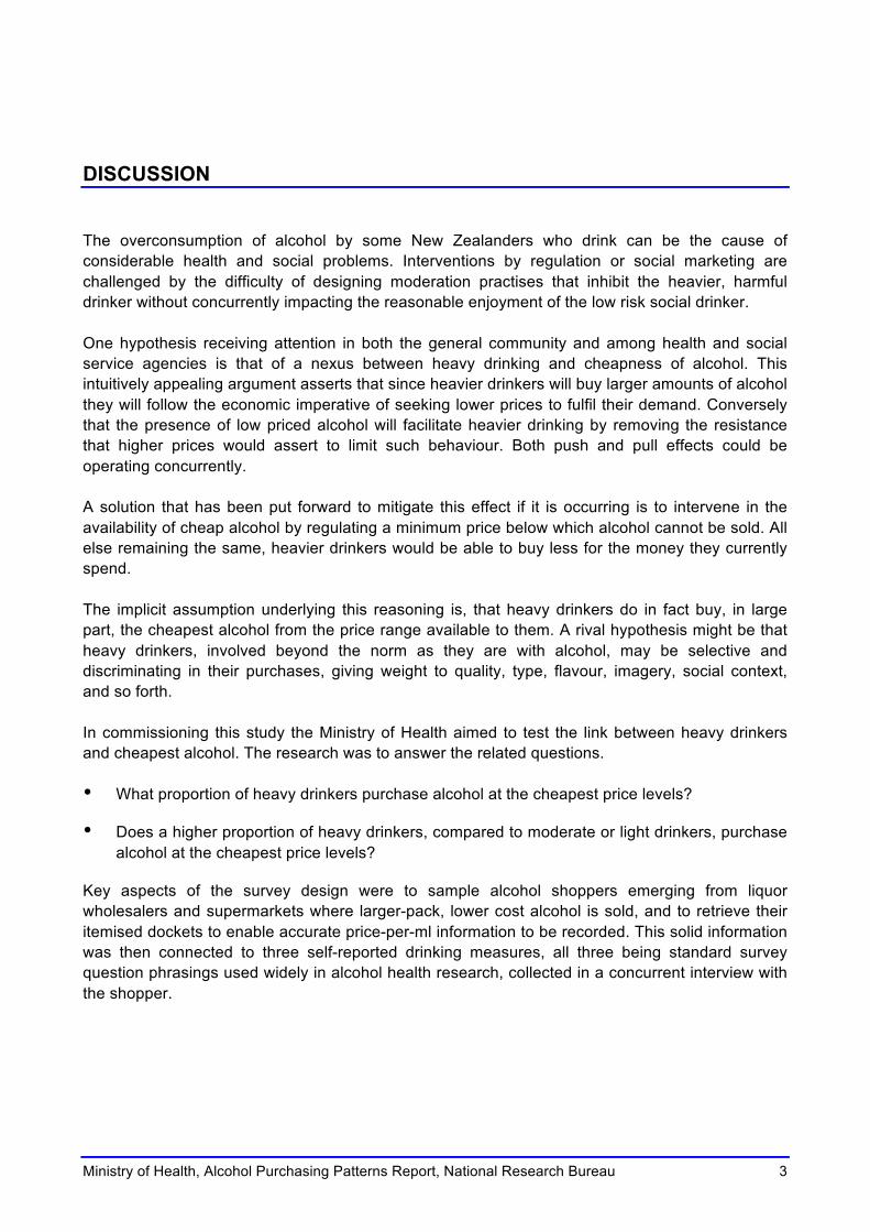
DISCUSSION The overconsumption of alcohol by some New Zealanders who drink can be the cause of considerable health and social problems. Interventions by regulation or social marketing are challenged by the difficulty of designing moderation practises that inhibit the heavier, harmful drinker without concurrently impacting the reasonable enjoyment of the low risk social drinker. One hypothesis receiving attention in both the general community and among health and social service agencies is that of a nexus between heavy drinking and cheapness of alcohol. This intuitively appealing argument asserts that since heavier drinkers will buy larger amounts of alcohol they will follow the economic imperative of seeking lower prices to fulfil their demand. Conversely that the presence of low priced alcohol will facilitate heavier drinking by removing the resistance that higher prices would assert to limit such behaviour. Both push and pull effects could be operating concurrently. A solution that has been put forward to mitigate this effect if it is occurring is to intervene in the availability of cheap alcohol by regulating a minimum price below which alcohol cannot be sold. All else remaining the same, heavier drinkers would be able to buy less for the money they currently spend. The implicit assumption underlying this reasoning is, that heavy drinkers do in fact buy, in large part, the cheapest alcohol from the price range available to them. A rival hypothesis might be that heavy drinkers, involved beyond the norm as they are with alcohol, may be selective and discriminating in their purchases, giving weight to quality, type, flavour, imagery, social context, and so forth. In commissioning this study the Ministry of Health aimed to test the link between heavy drinkers and cheapest alcohol. The research was to answer the related questions. • What proportion of heavy drinkers purchase alcohol at the cheapest price levels?

• Does a higher proportion of heavy drinkers, compared to moderate or light drinkers, purchase alcohol at the cheapest price levels?

Key aspects of the survey design were to sample alcohol shoppers emerging from liquor wholesalers and supermarkets where larger-pack, lower cost alcohol is sold, and to retrieve their itemised dockets to enable accurate price-per-ml information to be recorded. This solid information was then connected to three self-reported drinking measures, all three being standard survey question phrasings used widely in alcohol health research, collected in a concurrent interview with the shopper.


The study formed the price-per-ml observations collected into quintiles to provide a systematic dimension of the prices being paid, and then inspected each quintile for the presence of heavier drinkers. Of particular interest was whether heavier drinkers were a strong presence in the cheapest quintile and concurrently a weak presence in the progressively dearer quintiles. Each of the three questions generally accepted by researchers as reflecting the extent of a persons alcohol consumption were inspected across the price quintiles in turn. For each it emerged that those shoppers reporting the heaviest drinking were active across the price range, and were not the dominant group making up purchasers of the cheapest alcohol. This means that there are more moderate and lighter drinkers present in the lowest price decile than heavy drinkers. A strategy of raising the minimum retail price per standard drink (10mls of alcohol in NZ) would not impact the majority of heavy drinkers, and would impact more moderate and lighter drinkers than heavy drinkers. Of particular community concern is the purchasing of alcohol by the formative 18-24 year olds. While much of their drinking is known to occur in clubs and bars where the price per standard drink is at the highest, there is no support for the view that when buying packaged alcohol at supermarkets and liquor outlets, they take the least cost approach. The present study recorded a good size sub-sample of 18-24 year olds. Their purchasing was evident across all five quintiles of the price range, rather than imbalanced noticeably toward the least cost range. In this data is was those shoppers aged 65 years and over who had the highest proportionate inclination to purchase alcohol in the lowest price quintile. Considering ethnicities of alcohol shoppers, Pacific people at 24% were more likely than Maori at 22% or NZ European at 19% to purchase in the least cost price range. The differences are however, not of large magnitude. We inspected the types of alcohol drinks appearing at each price level to see whether least cost alcohol was strongly identified with a particular type of drink. The data from a wide cross section of buyers, buying from a wide cross section of stores, does not support such a connection. Beer, wine, spirits, and RTD's could each be seen to have been bought in considerable numbers in each quintile tier of price per ml of alcohol. An econometric multivariate analysis was undertaken to test for the presence of interactions amongst the measures which might lead to a different and more complex interpretation of what the bivariate analysis indicated. The estimated equations confirm the expected negative relationship between the price paid for alcohol and the quantity of alcohol consumed, that is suggested by the quintile analysis.


However, this relationship is not that of a normal demand curve where everyone pays the same price. The equations are probably picking up a product mix effect whereby higher prices are charged for, and paid by consumers for higher quality products – whether real or perceived, and such products are consumed in smaller quantities than cheaper products. Thus we cannot make the usual inference that higher prices at the cheaper end of the market would reduce the quantity consumed by the amount indicated by the elasticities. Clearly though (from Table 3), to the extent that there is any sort of demand response to higher prices, it will be dominated by consumers in the highest consumption quintile – in absolute quantity terms if not in proportional terms. A minimum price on the cheapest drinks that brought their price up to the Q1-Q2 boundary, would involve a price increase on those products of about 1.4c/ml or about 18% (ie, 14 cents per NZ standard drink). If the elasticity in Table 4 operated as a true price elasticity, the reduction in consumption of such drinks would be about 6.3%, or only about 1.5% in total. This is because even though the top consumption quintile purchases more of its alcohol from the lowest price quintile than does any other consumption quintile, the proportion of its consumption purchased from the lowest price quintile is still only around 27% (0.146/0.548). Expressed in reverse, 73% of the alcohol consumed by the highest consumption quintile is not purchased from the lowest price quintile. The results provide tentative evidence that the price of wine has a stronger influence on drinking intensity than the prices of spirits or beer, the latter two being more related to drinking frequency than drinking intensity. In overview, it would be fair to infer from these findings that considerations other than heavy drinking explain least cost purchasing, and conversely considerations other than least cost drive heavy drinking. Among these may be affordability, cost conscious prudence, low attachment to brand imagery, low attachment to so called quality, the intended context of consuming it, and other factors.


A. BACKGROUND One of the specific objectives of the National Drug Policy 2007-2012 is to reduce harm to individuals, families and communities from the risky consumption of alcohol. To this end a research project relating to the purchasing patterns of New Zealand drinkers was proposed. B. OBJECTIVES The research project was planned to answer the following research questions: • What proportion of heavy drinkers purchase alcohol at the cheapest price levels?

• Does a higher proportion of heavy drinkers, compared to moderate or light drinkers, purchase alcohol at the cheapest price levels?


C. METHOD 1. OPERATIONAL DEFINITION OF THE TERMS Operational definitions of three key terms were formed. These terms were, heavy drinkers, cheap(est) price and purchasing. a. Heavy Drinkers When survey interviews are used to obtain self-reports on drinking, the result is a relative scale rather than an absolute one. By this we are acknowledging that interview questions can distribute people into heavier, moderate and lighter drinkers along a relative continuum but can't readily state the volume of alcohol in mls that each point in the continuum represents. Alcohol survey research such as the Ministry of Health's NZHS and ADUS have settled on three questions which are relied on to differentiate each persons (respondents) relative use of alcohol. These questions do not prompt or assist the respondent with showcards of standard drinks, or define the quantity of a "drink". The phrasing of the three questions is shown in the attached questionnaire. The survey analysis made constructive use of the continuum of drinking as expressed in the three standard questions, but can also be read from a threshold approach. Specifically heavy drinkers for the frequency of drinking question are those who consume alcohol four times a week or more. Heavy drinkers for the question on how many drinks they have on a day that they do drink are those who take 10 or more drinks on such a day. Finally heavy drinkers for the question on how often they have five or more drinks on the same occasion are those who do so three or more times a week. The questions entail the opportunity to then combine them by a simple multiplication to give each alcohol buyer a relative "drinks per month" figure for drinking intensity. This gives the analysis the freedom to define and redefine "heavy" drinker quite flexibly in examining the connection with price paid.


b. Cheap(est) Price For Alcohol Given that alcohol strength, pack size, type of alcohol, quantity per pack, discounting and specials can influence the price, it is necessary to convert purchases item by item into mls of alcohol. Fortunately receipts for purchase identify brand, quantity and price so that the successive items listed on a sale docket can be converted to "cents per ml of alcohol" using the alcohol percentage and litre content of that item stated on the label. It is important to recognise that retailing activity like 'specials' and store vs store competition mean we need to define cheapest in relation to the store and the day of purchase. The initial approach was to obtain and convert into cents per ml each of the purchases shown on the docket of each customer emerging from a supermarket or liquor wholesaler, as the first step. The second step was to check that specific store's shelf prices to code the items individually as to whether they were, or were not, the cheapest available to the customer on the day at that store. This too being done on a cost per ml of alcohol basis. This second step was subsequently displaced by using the lowest (bracket of) actual prices paid by purchasers. The presence of poorly patronised brands, run-out stock sales, and deep specialing on launch-phase lines suggested the literal cheapest item of the day was a poor reflection of the lowest-price behaviour of the alcohol shoppers.


c. Purchaser Vs Drinker A challenge facing this research project was that of dealing with the overlap of purchaser and drinker. The take-home purchaser may not drink all that he/she buys. Conversely the drinker often does not buy all the alcohol they consume. These are specially true of the supermarket and liquor wholesale outlets that provide the lower-priced options to the public. (Bars, clubs, restaurants and on-premise drinking implies significantly dearer alcohol options and for that reason are not included in this study). In a theoretical but impractical option the researcher would screen among drinkers to find a sample of "heavy" drinkers and get them to retain their purchasing invoices and then match these invoices to the prevailing prices within the stores from which they had purchased, or more effectively against the lowest prices paid across the prevailing market. More realistic in the sense of being achievable in practise, is to intercept purchasers exiting liquor wholesalers and supermarkets, obtain their dockets, and ask their drinking intensity using the questions in Appendix 1. This enables the study to calculate the cost per ml of alcohol they paid and determine where on the range of prevailing real prices paid, that falls. A 'soft' resolution of the overlap problem would be to ask the purchaser whether the greater part of their purchases were to be consumed by themselves or by others – and if others (or an other), to give indications of that/those others drinking frequencies also. The analysis can then be done by: i. First, including only those who were buying "mainly for themselves" in the dataset. ii. Then, adding back into the dataset those buying for "mainly for others" and seeing if any

different conclusion resulted. When we include all buyers in the dataset scenario we are effectively analysing whether light/moderate/heavy drinkers are buying at the cheapest price, regardless of whether they are going to drink it themselves or serve/provide it to others. This is the predominant thrust of the analysis of this study. Analysis of this question for the present survey established that the percentage buying "mainly for others" was very small at 6%. Their impact on the finding of the survey was considered too small to influence the general inferences and conclusions drawn. While an argument might be made that reciprocally they benefit from others purchasing for them in turn, this is uncertain. With the advantage of hindsight it may be best to simply screen out the small number of buyers who are buying "mostly for others" from similar studies in future.


2. CHOICE OF METHOD In this section we consider the two methods available to collect data for answering the question. We have a choice between taking recalled purchasing, eg, in a phone or doorstep interview at the home on the one hand, and observed purchasing, eg, in an exit interview at wholesalers and supermarkets at the time of purchase, on the other. The recall interview at the home (whether on phone or doorstep) carries drawbacks both specific to the dependent variable and generic to the approach. With respect to the specific drawback, people may not be conscious that they are buying at the least-cost. This may be an option they have drifted into to suit their circumstances. The home interview would therefore have to rely increasingly on recall of products purchased and price paid at past purchase occasions to see whether and to what extent the person was a lowest-cost buyer. Alcohol recall is substantially compromised by social desirability bias as well as forgetting and selective recall. We felt purchase reports would be compromised by a recall approach. The number of interviews that could be performed if interviews are at household doorsteps was very likely much smaller than would support good analysis, given the budget available. If phone, the response rate for phone surveys has fallen to very low levels in recent years, giving rise to reservations about the representativeness of those who do participate, even if basic demographics are "balanced" by quotas or weighting. The exit interview conducted at the point of purchase and thereby at the time of purchase provides more robust data for identifying and qualifying least-cost purchasing. The strategy is to station interviewers at a selection of alcohol outlets who intercept exiting shoppers and administer a short interview. During this interview the shopper is offered a small gift voucher on behalf of the researcher to provide their itemised docket to the survey and to also answer the drinking questions required for analysis. This approach gives sound information about the purchases and what they cost by way of the docket. The one form of purchasing not covered by the exit interview is on-line purchasing via the Internet. Options to source this segments purchasing are phone or personal visits at home, or the use of an online consumer panel. Neither gives us direct access to real-cost information in the way that the exit interview does. The price actually paid is compromised by forgetting, unless the respondent can be persuaded to retrieve their online order – a type of task for which there is generally little co-operation in householder surveys. Where a given purchase or purchasers overall basket of purchases fell in the cost per ml of alcohol prevailing range, would be difficult to determine reliably.


3. SURVEY SAMPLE Liquor wholesalers and supermarkets are observably the retail outlets offering the greatest volume sales of alcohol as also the most competitive prices. Any relationship between heavy drinking and least-cost purchasing would need to show up among customers of these outlets to be of importance. Two stage random selection for the sampling of customers would best be applied to: • The selection of liquor stores and of supermarkets respectively.

• The customer emerging from the stores, with the intent that sampling effort be applied roughly proportional to customer flow.

There is no administrative data by which to structure the sample formally and budget did not allow for developing one, even were this feasible. However, the sample of exit customers can be an acceptable basis for generalising any relationship found between least-cost purchasing and heavy drinking. The relationship can be looked at separately for supermarket customers and liquor store customers as well as overall. In practice the use of exit interviews requires permissioning from the management of the retail organisation. Supermarket and liquor stores of significant size and therefore trading area are virtually all now part of chains with centralised marketing. Some of these have blanket protocols precluding survey work from being done among their shoppers. Permission was obtained from a spread of 10 large-footprint supermarkets for interviewing shifts to take place in their carpark areas. These were located as follows: Central Auckland Hamilton Central South Auckland Hamilton South East East Auckland Hamilton South Auckland North Christchurch North Christchurch West Dunedin The sample plan was to include a North Island metropolitan and large provincial, and a South Island metropolitan and large provincial. Thus Auckland as the largest North Island metropolitan, rather than Wellington was chosen.


Similarly permission was obtained to interview at 25 liquor stores. The footprint of a liquor wholesaler is typically much smaller than that of a supermarket, calling for lower concentration of the sample obtained at each store. The smaller sample per store also recognised that managements wish to avoid a heavy interviewing presence at the store. Liquor outlet sampling took place in the following areas: Auckland East Wellington Auckland West Lower Hutt Auckland North Upper Hutt Tauranga, Mt Maunganui Wanganui Hamilton Wanganui Hamilton East New Plymouth Hamilton North New Plymouth Christchurch Hastings Christchurch Napier Gisborne Sampling of both liquor wholesalers and supermarkets, while purposively selected to represent a socio-economic spread and relatively large footprints, cannot be viewed in terms of a finite probability of selection, either at the store level or respondent level.


4. INTERVIEWING The ideal exit interview sample is one for which every xth shopper emerging from the store is intercepted, screened for eligibility, ie, bought an alcohol product, and then recruited into the interview. In practise this is very difficult to achieve with the latitude allowed the interviewers by store management, and without a very large interviewer team. For this survey interviewers approached shoppers with the purposive consideration of including men and women, and people judged by eye to be aged up to 34 years, 35-54 years and 55 and over, in broadly equal proportions, relaxing this general specification to conform to the observed mix of the shoppers age/gender at the particular site. The profile of the achieved sample of 2,000 is shown below. Gender Liquor Store Supermarket Total %

Female 398 524 922 46.1

Male 607 471 1,078 53.9

1,005 995 2,000 100

Ethnicity Liquor Store Supermarket Total %

NZ European 618 720 1,338 66.9

Maori 228 89 317 15.9

Pacific 51 60 111 5.5

Asian 42 52 94 4.7

Other 66 72 140 7.0

1,005 995 2,000 100

Age Group Liquor Store Supermarket Total %

Up to 24 years 262 57 319 15.9

25 to 34 years 208 150 358 17.9

35 to 44 years 191 217 408 20.4

45 to 54 years 165 222 387 19.4

55 to 64 years 116 194 310 15.5

65+ years 63 155 218 10.9

1,005 995 2,000 100

Liquor shoppers in this purposively conceived and controlled sample conform in broad terms to the general population along the demographics collected, indicating perhaps no more than that shopping for alcohol is a common population behaviour.


5. INTERVIEWING PROCEDURE Shoppers were approached face-to-face by interviewers wearing NRB photo identity badges and asked whether they had purchased beer, wine or spirits on this particular visit to the store. Where they affirmed they had done so they were told the survey offered a gift ($5 in an envelope) in exchange for their invoice and the answering of a short interview. Those who agreed proceeded to hand over their receipt, receive the gift, and answer the questionnaire. Response rates were not recorded but interviewers noted that refusals were rare and generally resulted from the person having run out of time, rather than any reaction to the topic or questions.


D. FINDINGS: BI-VARIATE PERCENTAGED ANALYSIS 1. THE TERM WEIGHTED AVERAGE PRICE, DEFINED The term weighted average is used here to refer to the price per ml of alcohol paid by the shopper when the volumes and alcohol strengths of all the items he/she purchased on the surveyed occasion are taken together. For example, a shopper may have purchased a 700ml bottle of wine of 10% alcohol strength for $7, giving a price per ml of alcohol of 10¢ for that item. In addition, they may have purchased on the same occasion a 3 litre cask of wine of 10% alcohol strength for $15, giving a price of 5¢ per ml of alcohol for that item. The weighted average paid for alcohol on that shopping trip is found as 2,200 cents/370mls = 5.59 cents per ml. Since the NZ Standard drink is defined as 10mls of alcohol, this translates to 37 NZ standard drinks at 55.9 cents per standard drink. The merit for inspecting self reported level of alcohol consumption in terms of weighted average price per ml of alcohol paid is that it overcomes the limitation of looking only at whether the person did or did not buy the cheapest alcohol available – seen in isolation the presence or absence of the cheapest item in their shopping might mask the true price per ml at which they are drinking.


2. THE USE OF QUINTILES IN THE ANALYSIS Once each alcohol shoppers purchase invoices had been converted to weighted average paid per ml of alcohol, shoppers were then rank ordered from those who had paid the least to those who had paid the most per ml. Prices paid in cents per ml ranged from a low of just below 5 cents to a high of just above 56 cents. For a NZ standard drink this converts simply to 50 cents per drink to $5.60 per drink. For conceptual and practical reasons the analysis needed to form a variable from this range that would provide a continuum ranging from those who paid the least through those who paid in the middle range, to those who paid the most per ml of alcohol bought. Given the sample size of 2,000 shoppers available it was deemed suitable to identify those shoppers paying in the lowest 20% range as the "lowest cost purchasers". This meant the sample base for this group would still be a stable number of 400 respondents for inspection. By extension the 20% quintiles would provide five points along the price-paid continuum to inspect the relationship with drinking frequency, intensity and price bracket shopped in. The quintiles revealed by the survey are expressed below in price per ml and in NZ standard drinks.

Respondent Quintile

Cost per millilitre of pure alcohol

Cost per NZ standard drink

Lowest 4.57¢ - 9.13¢ 46¢ - 91¢

2 9.15¢ - 10.19¢ 92¢ - $1.02

3 10.21¢ - 11.35¢ $1.02 - $1.14

4 11.36¢ - 13.86¢ $1.14 - $1.39

Highest 13.88¢ - 56.66¢ $1.39 - $5.67

In New Zealand, a standard drink is defined as a drink containing 10mls of pure alcohol. Results have been rounded to the nearest cent.


Monthly Fortnightly Weekly 2-3 per week

4-5 per week

Daily plus0%

10%

20%

30%

Alc

ohol

Sho

pper

s

Drinking Frequency

20%

14% 15%20%

23% 25%

3. FREQUENCY OF DRINKING BEER, WINE OR SPIRITS VIEWED AGAINST PRICE PER

ML ALCOHOL PAID One of the three questions recurringly used by alcohol researchers to mark the respondents drinking, is simply to ask how often they have a drink of beer, wine or spirits. The answer is taken open ended, without reading out options or showing a card. Below we examine whether more frequent drinking is associated with more commonly purchasing in the lowest quintile price per ml alcohol. Figure 1: Proportion Of Alcohol Shoppers (vertical) Of Each Drinking Frequency Who Purchased In The Cheapest Cost Per Ml Alcohol Quintile (figures rounded)

Bases: 109 93 384 702 278 397 The strength of the relationship can be assessed by noting the departure from the 20% broken line. This figure shows that as drinking frequency increases, the proportion of drinkers who buy in the cheapest quintile of alcohol price rises. Given that only 25% of most frequent drinkers appear among the cheapest buying quintile we may view the relationship as not particularly strong, ie, 75% of the heaviest drinkers are paying more than the lowest cost range.


Lowest Quintile

(cheapest)

2ndQuintile

3rdQuintile

4thQuintile

Highest Quintile

(dearest)

0%

10%

20%

30%

% O

f Dai

ly P

lus

Drin

kers

Price Per Ml Quintiles

25%

17%21% 20%

16%

Following through on the most frequent drinkers we see them appearing in all five quintiles of purchase price at proportions not far different to an even spread, viz buying at all price levels relatively evenly. Figure 2: The Price-Per-Ml Quintiles (horizontal) In Which The Most Frequent Drinkers (ie, Daily Plus), Buy (figures rounded), Base = 397

This profile shows the most frequent drinkers purchasing in all price ranges, with a moderate emphasis on the cheapest at the expense of the dearest.


1 or 2 3 or 4 5 or 6 7 to 9 10 or more0%

10%

20%

30%

% B

uyin

g In

The

Che

apes

t Qui

ntile

Drinks Per Day, When Drinking

21%17% 18%

23%26%

4. NUMBER OF DRINKS ON A TYPICAL DAY WHEN DRINKING ALCOHOL Another question recurringly used in alcohol research is that which asks the survey respondent how many drinks of wine/beer/spirits they have a on typical day when they are drinking. Where needed a drink is referred to as a glass or can, as appropriate to the drink. No showcard is proffered but where the respondent appears non-plussed in arriving at their answer, the options are read out to assist. Below we examine whether drinking more drinks on a typical drinking day correlates with purchasing in the lowest quartile of purchase prices. Figure 3: Proportion Of Drinkers Who Purchased In The Cheapest Cost Per Ml Of Alcohol (horizontal) (percentages rounded)

Bases: 686 509 310 160 297 The figure shows a definite inclination for the proportion of drinkers in progressively higher "drinks per drinking day" groups to buy within the lowest price quintile more often than moderate or lighter drinkers do. The effect however, is not quantitatively strong.


Lowest Quintile

(cheapest)

2ndQuintile

3rdQuintile

4thQuintile

Highest Quintile

(dearest)

0%

10%

20%

30%

Perc

ent O

f The

10

Plus

Per D

ay D

rinke

rs

Price Quintiles

26%23% 21% 21%

9%

Following through on those who drink the largest number of drinks on the days when they do drink, ie, the "10 or more" column on the right of the figure above, we see that with the exception of the dearest quintile of prices, these drinkers are to be found buying in all price ranges. Figure 4: The Price-Per-Ml Quintiles (horizontal) In Which Those Who Drink 10 Or More Drinks On A Typical Day When Drinking, Buy Alcohol (horizontal), Base = 297 (figures rounded)

This profile shows that those in the group who have the highest number of drinks on a day when they are drinking, buy from within all of the price ranges. They tend to avoid the dearest price range in a step wise drop, appearing instead more commonly in each of the other price ranges, particularly in the cheapest.


Never Less than monthly

Monthly Fortnightly Weekly Twice a week

3-4 per week

Daily0%

10%

20%

30%

% W

ho B

ough

t In

The

Chea

pest

Qui

ntile

Frequency Of Drinking Five Plus Per Day

19% 19% 17% 17%22%

27% 26%29%

5. FIVE OR MORE DRINKS ON ONE OCCASION A third question recurringly used in alcohol research is to ask survey respondents how often they have five or more drinks on one occasion. The interviewer can also record a refused and a don't know option. Below we examine whether the frequency with which people drink five or more drinks on an occasion correlates with the price range within which they purchase alcohol. Figure 5: Proportion Of Drinkers (vertical) Of Each "5 Plus Per Occasion" Frequency (horizontal) Who Purchased In The Cheapest Cost Per Ml Of Alcohol, Quintile (figures rounded)

Bases: 403 320 276 229 481 33 144 75 The figure shows that there is clear upturn in the proportion of five plus per occasion drinkers who make their alcohol purchases down in the cheapest quintile of alcohol prices. However, even among the most avid of these drinkers the greater percentage are buying in higher cost quintiles.


Lowest Quintile

(cheapest)

2ndQuintile

3rdQuintile

4thQuintile

Highest Quintile

(dearest)

0%

10%

20%

30%

% O

f Bin

ge D

rinke

rs B

uyin

g

Price Quintiles

27%

21% 20%17% 16%

Following through on the two most avid groups (3-4 per week and daily) in the above table, combined for this purpose, we see a similar effect. With the exception of the two highest quintiles of price, these drinkers are represented in proportions not greatly different to the 20% that might be expected if they were purchasing evenly across the price range. Figure 6: The Price Per Ml Quintiles In Which Those Who Binge Drink 3 Or More Times A Week, Buy Alcohol (figures rounded), Base 219

The figure shows that those binge drinking most frequently favour the cheapest quintile in the price range at the expense of the dearest quintile to a perceptible extent, but the predominant picture is of this group buying relatively evenly across the price range.


NZ European

Maori Pacic Asian Other0%

10%

20%

30%

% O

f Alc

ohol

Sho

pper

s

Ethnicity Of Alcohol Shopper

19%22% 24%

17%22%

6. PRICES PAID BY ETHNIC GROUPS Figure 7 below shows the percentage of each ethnic group purchasing alcohol in the cheapest quintile. Figure 7: Percent Of Shoppers Within Each Ethnicity Group Who Bought In The Cheapest Quintile

Pacific people were more inclined to purchase in the cheapest quintile than other ethnic groups, as were Maori to a lesser extent. These two groups are markedly underrepresented in the dearest quintiles, with relatively higher representation spread over the other four quintiles.


7. ALCOHOL TYPES PURCHASED IN EACH PRICE QUINTILE The 2,000 shoppers interviewed had purchased 2,714 'items' defined as charged line items on their invoices. The figures below show how often each of the alcohol types appeared in each price quintile of items.

Cheapest Quintile 2nd Quintile 3rd Quintile 4th Quintile

Dearest Quintile

Cider 0 1 5 11 19

0% <1% 1% 2% 3%

Beer 136 222 267 228 120

25% 41% 49% 42% 22%

Wine 248 196 178 195 240

46% 36% 33% 36% 44%

Spirits 37 25 23 42 41

7% 5% 4% 8% 8%

RTD's 122 99 70 67 123

22% 18% 13% 12% 23%

BASE 543 543 543 543 543

Wine, thanks to some extent to the lower price of cask wine, and RTD's, are notable in having a disproportionate presence in the cheapest quintile, relative to the other quintiles. These two products also appear strongly in the dearest quintile, a reflection of the way variants of them are price positioned to the consumer.


Lowest Quintile

(cheapest)

2ndQuintile

3rdQuintile

4thQuintile

Highest Quintile

(dearest)

0%

10%

20%

30%

Volu

me

Perc

ent

Of T

heir

Purc

hase

s

Price Quintiles

30%25%

22%19%

5%

8. THE VOLUME OF ALCOHOL BOUGHT IN THE LOWEST PRICE QUINTILE, BY

DRINKERS OF VARIOUS FREQUENCY More frequent drinkers, heavier per-occasion drinkers, and more frequent binge drinkers were earlier shown to participate in price-per-ml alcohol relatively evenly over the price range except for some disproportion at the extremes of price. In brief they are not confined to least cost purchasing of alcohol. That "price participation" approach however leaves open the possibility that when heavy drinkers do make use of low cost, they purchase a disproportionately larger volume proportion of their requirements, than do lighter or moderate drinkers, when purchasing at low prices. Figure 8: Comparing The Proportion Of Their Alcohol Purchased At The Different Price Quintiles, For People Who Drink 10+ Drinks On A Typical Day They Do Drink Base: Volume in mls, 66,532 mls, purchased by "10 plus per typical day when drinking" shoppers (figures rounded)

This heaviest drinker group do show a clear tendency toward buying a greater proportion of their volume at the cheapest end, but largely at the singular expense of the dearest products. Much of their purchasing is done across the middle price ranges.


9. PERCENTAGED TABLES

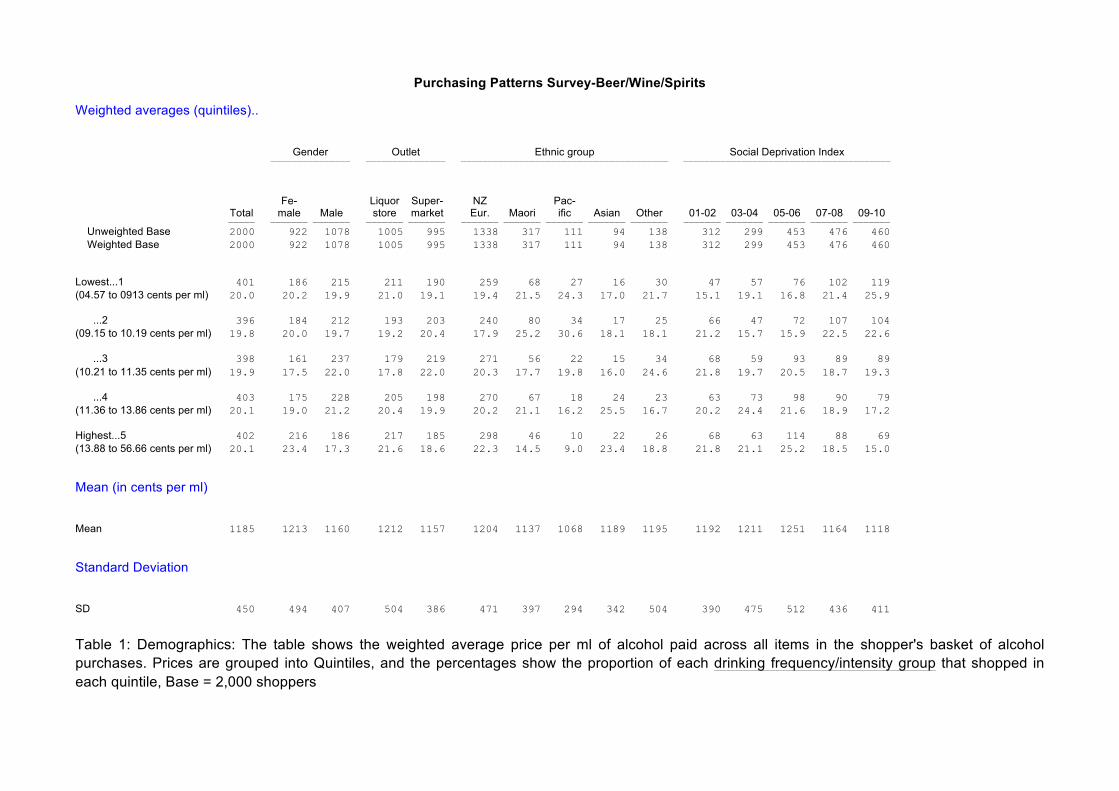
Purchasing Patterns Survey-Beer/Wine/Spirits Weighted averages (quintiles).. Gender Outlet Ethnic group Social Deprivation Index ——————————————— ——————————————— ——————————————————————————————————————— ——————————————————————————————————————— Fe- Liquor Super- NZ Pac- Total male Male store market Eur. Maori ific Asian Other 01-02 03-04 05-06 07-08 09-10 ————— ——————— ——————— ——————— ——————— ——————— ——————— ——————— ——————— ——————— ——————— ——————— ——————— ——————— ——————— Unweighted Base 2000 922 1078 1005 995 1338 317 111 94 138 312 299 453 476 460 Weighted Base 2000 922 1078 1005 995 1338 317 111 94 138 312 299 453 476 460 Lowest...1 401 186 215 211 190 259 68 27 16 30 47 57 76 102 119 (04.57 to 0913 cents per ml) 20.0 20.2 19.9 21.0 19.1 19.4 21.5 24.3 17.0 21.7 15.1 19.1 16.8 21.4 25.9 ...2 396 184 212 193 203 240 80 34 17 25 66 47 72 107 104 (09.15 to 10.19 cents per ml) 19.8 20.0 19.7 19.2 20.4 17.9 25.2 30.6 18.1 18.1 21.2 15.7 15.9 22.5 22.6 ...3 398 161 237 179 219 271 56 22 15 34 68 59 93 89 89 (10.21 to 11.35 cents per ml) 19.9 17.5 22.0 17.8 22.0 20.3 17.7 19.8 16.0 24.6 21.8 19.7 20.5 18.7 19.3 ...4 403 175 228 205 198 270 67 18 24 23 63 73 98 90 79 (11.36 to 13.86 cents per ml) 20.1 19.0 21.2 20.4 19.9 20.2 21.1 16.2 25.5 16.7 20.2 24.4 21.6 18.9 17.2 Highest...5 402 216 186 217 185 298 46 10 22 26 68 63 114 88 69 (13.88 to 56.66 cents per ml) 20.1 23.4 17.3 21.6 18.6 22.3 14.5 9.0 23.4 18.8 21.8 21.1 25.2 18.5 15.0

Mean (in cents per ml) Mean 1185 1213 1160 1212 1157 1204 1137 1068 1189 1195 1192 1211 1251 1164 1118

Standard Deviation SD 450 494 407 504 386 471 397 294 342 504 390 475 512 436 411 Table 1: Demographics: The table shows the weighted average price per ml of alcohol paid across all items in the shopper's basket of alcohol purchases. Prices are grouped into Quintiles, and the percentages show the proportion of each drinking frequency/intensity group that shopped in each quintile, Base = 2,000 shoppers

Purchasing Patterns Survey-Beer/Wine/Spirits Weighted averages (quintiles).. Q3 How often would have wine/beer/spirits Q4 Number of drinks on typical day Q5 How often have 5+ drinks on one occasion ————————————————————————————————————————— —————————————————————————————————— —————————————————————————————————————————————————————————————— Daily, Fort- 2 or 3 4 or 5 6 or 7 Less Fort- W'ends 3 or 4 Daily/ Mon- night- Once times times times 10 or than night- /twice times almost DK/ Total thly ly a week a week a week a week 1 or 2 3 or 4 5 or 6 7 to 9 more Never mnthly Mnthly ly Weekly a week a week daily ref. ————— —————— —————— —————— —————— —————— —————— —————— —————— —————— —————— —————— —————— —————— —————— —————— —————— —————— —————— —————— —————— Unweighted Base 2000 109 93 384 702 278 397 686 509 310 160 297 403 320 276 229 481 33 144 75 4 Weighted Base 2000 109 93 384 702 278 397 686 509 310 160 297 403 320 276 229 481 33 144 75 4 Lowest...1 401 22 13 59 138 63 100 141 84 56 36 78 75 60 48 38 104 9 38 22 1 (04.57 to 0913 cents per ml) 20.0 20.2 14.0 15.4 19.7 22.7 25.2 20.6 16.5 18.1 22.5 26.3 18.6 18.8 17.4 16.6 21.6 27.3 26.4 29.3 25.0 ...2 396 18 11 79 147 61 68 112 96 76 32 67 73 43 61 39 120 4 29 16 0 (09.15 to 10.19 cents per ml) 19.8 16.5 11.8 20.6 20.9 21.9 17.1 16.3 18.9 24.5 20.0 22.6 18.1 13.4 22.1 17.0 24.9 12.1 20.1 21.3 0.0 ...3 398 16 22 78 142 53 84 141 101 57 35 61 74 67 49 54 97 8 28 16 2 (10.21 to 11.35 cents per ml) 19.9 14.7 23.7 20.3 20.2 19.1 21.2 20.6 19.8 18.4 21.9 20.5 18.4 20.9 17.8 23.6 20.2 24.2 19.4 21.3 50.0 ...4 403 23 22 93 135 43 80 128 112 60 33 63 80 69 56 49 100 5 23 14 0 (11.36 to 13.86 cents per ml) 20.1 21.1 23.7 24.2 19.2 15.5 20.2 18.7 22.0 19.4 20.6 21.2 19.9 21.6 20.3 21.4 20.8 15.2 16.0 18.7 0.0 Highest...5 402 30 25 75 140 58 65 164 116 61 24 28 101 81 62 49 60 7 26 7 1 (13.88 to 56.66 cents per ml) 20.1 27.5 26.9 19.5 19.9 20.9 16.4 23.9 22.8 19.7 15.0 9.4 25.1 25.3 22.5 21.4 12.5 21.2 18.1 9.3 25.0

Mean (in cents per ml) Mean 1185 1204 1303 1233 1182 1168 1119 1215 1214 1181 1154 1083 1220 1237 1216 1204 1137 1189 1114 1041 1050

Standard Deviation SD 450 403 581 519 438 440 377 491 445 453 443 346 438 509 494 450 436 500 355 246 406 Table 2: Drinking Behaviour: The table shows the weighted average price per ml of alcohol paid across all items in the shopper's basket of alcohol purchases. Prices are grouped into Quintiles, and the percentages show the proportion of each demographic group that shopped in each quintile, Base = 2,000 shoppers

Purchasing Patterns Survey-Beer/Wine/Spirits Weighted averages (quintiles).. QF Day of purchase QA Age group ——————————————————————————————— ——————————————————————————————————————————————— Sunday to Thurs- Satur- Up to 25-34 35-44 45-54 55-64 65+ Total Wed'day day Friday day 24 yrs yrs yrs yrs yrs yrs ————— ——————— ——————— ——————— ——————— ——————— ——————— ——————— ——————— ——————— ——————— Unweighted Base 2000 391 351 565 693 319 358 408 387 310 218 Weighted Base 2000 391 351 565 693 319 358 408 387 310 218 Lowest...1 401 78 77 108 138 74 61 75 69 57 65 (04.57 to 0913 cents per ml) 20.0 19.9 21.9 19.1 19.9 23.2 17.0 18.4 17.8 18.4 29.8 ...2 396 74 74 98 150 66 55 90 76 70 39 (09.15 to 10.19 cents per ml) 19.8 18.9 21.1 17.3 21.6 20.7 15.4 22.1 19.6 22.6 17.9 ...3 398 71 72 113 142 48 81 78 91 61 39 (10.21 to 11.35 cents per ml) 19.9 18.2 20.5 20.0 20.5 15.0 22.6 19.1 23.5 19.7 17.9 ...4 403 92 57 119 135 68 88 78 79 58 32 (11.36 to 13.86 cents per ml) 20.1 23.5 16.2 21.1 19.5 21.3 24.6 19.1 20.4 18.7 14.7 Highest...5 402 76 71 127 128 63 73 87 72 64 43 (13.88 to 56.66 cents per ml) 20.1 19.4 20.2 22.5 18.5 19.7 20.4 21.3 18.6 20.6 19.7

Mean (in cents per ml) Mean 1185 1173 1176 1216 1169 1201 1211 1184 1174 1191 1130

Standard Deviation SD 450 413 469 480 435 520 441 455 393 463 420 Table 3: Whether least cost shopping is greater on different days of the week, or differs by the age group of the shopper

Purchasing Patterns Survey-Beer/Wine/Spirits Individual invoice items (quintiles).. Gender Outlet Ethnic group Social Deprivation Index ——————————————— ——————————————— ——————————————————————————————————————— ——————————————————————————————————————— Fe- Liquor Super- NZ Pac- Total male Male store market Eur. Maori ific Asian Other 01-02 03-04 05-06 07-08 09-10 ————— ——————— ——————— ——————— ——————— ——————— ——————— ——————— ——————— ——————— ——————— ——————— ——————— ——————— ——————— Unweighted Base 2714 1283 1431 1293 1421 1846 408 141 107 210 472 409 608 624 570 Weighted Base 2714 1283 1431 1293 1421 1846 408 141 107 210 472 409 608 624 570 Lowest...1 541 269 272 264 277 344 99 33 20 44 80 71 95 138 151 (04.57 to 0913 cents per ml) 19.9 21.0 19.0 20.4 19.5 18.6 24.3 23.4 18.7 21.0 16.9 17.4 15.6 22.1 26.5 ...2 545 254 291 222 323 354 98 40 20 33 102 83 108 120 127 (09.15 to 10.19 cents per ml) 20.1 19.8 20.3 17.2 22.7 19.2 24.0 28.4 18.7 15.7 21.6 20.3 17.8 19.2 22.3 ...3 543 236 307 257 286 371 71 34 17 50 94 82 121 126 113 (10.21 to 11.35 cents per ml) 20.0 18.4 21.5 19.9 20.1 20.1 17.4 24.1 15.9 23.8 19.9 20.0 19.9 20.2 19.8 ...4 540 251 289 261 279 367 87 20 25 40 97 94 125 126 93 (11.36 to 13.86 cents per ml) 19.9 19.6 20.2 20.2 19.6 19.9 21.3 14.2 23.4 19.0 20.6 23.0 20.6 20.2 16.3 Highest...5 545 273 272 289 256 410 53 14 25 43 99 79 159 114 86 (13.88 to 56.66 cents per ml) 20.1 21.3 19.0 22.4 18.0 22.2 13.0 9.9 23.4 20.5 21.0 19.3 26.2 18.3 15.1

Mean (in cents per ml) Mean 1220 1239 1203 1270 1175 1237 1172 1093 1205 1259 1217 1247 1299 1202 1140

Standard Deviation SD 526 563 491 601 443 533 530 334 363 616 449 609 584 509 467 Table 4: Demographics: The table shows the price per ml of alcohol paid on an item by item basis, Base = 2,714 items purchased

Purchasing Patterns Survey-Beer/Wine/Spirits Individual invoice items (quintiles).. Q3 How often would have wine/beer/spirits Q4 Number of drinks on typical day Q5 How often have 5+ drinks on one occasion ————————————————————————————————————————— —————————————————————————————————— —————————————————————————————————————————————————————————————— Daily, Fort- 2 or 3 4 or 5 6 or 7 Less Fort- W'ends 3 or 4 Daily/ Mon- night- Once times times times 10 or than night- /twice times almost DK/ Total thly ly a week a week a week a week 1 or 2 3 or 4 5 or 6 7 to 9 more Never mnthly Mnthly ly Weekly a week a week daily ref. ————— —————— —————— —————— —————— —————— —————— —————— —————— —————— —————— —————— —————— —————— —————— —————— —————— —————— —————— —————— —————— Unweighted Base 2714 135 120 508 933 409 563 980 729 403 198 358 558 454 397 321 612 42 190 92 6 Weighted Base 2714 135 120 508 933 409 563 980 729 403 198 358 558 454 397 321 612 42 190 92 6 Lowest...1 541 32 15 88 181 92 126 196 123 78 45 92 106 80 77 54 134 9 46 27 1 (04.57 to 0913 cents per ml) 19.9 23.7 12.5 17.3 19.4 22.5 22.4 20.0 16.9 19.4 22.7 25.7 19.0 17.6 19.4 16.8 21.9 21.4 24.2 29.3 16.7 ...2 545 16 18 93 189 94 120 196 127 95 35 76 111 72 79 57 149 8 36 18 2 (09.15 to 10.19 cents per ml) 20.1 11.9 15.0 18.3 20.3 23.0 21.3 20.0 17.4 23.6 17.7 21.2 19.9 15.9 19.9 17.8 24.3 19.0 18.9 19.6 33.3 ...3 543 20 25 108 199 76 111 179 154 78 50 79 92 88 83 69 133 10 40 24 1 (10.21 to 11.35 cents per ml) 20.0 14.8 20.8 21.3 21.3 18.6 19.7 18.3 21.1 19.4 25.3 22.1 16.5 19.4 20.9 21.5 21.7 23.8 21.1 26.1 16.7 ...4 540 36 32 110 181 65 105 177 163 81 33 75 109 98 75 75 116 6 36 14 0 (11.36 to 13.86 cents per ml) 19.9 26.7 26.7 21.7 19.4 15.9 18.7 18.1 22.4 20.1 16.7 20.9 19.5 21.6 18.9 23.4 19.0 14.3 18.9 15.2 0.0 Highest...5 545 31 30 109 183 82 101 232 162 71 35 36 140 116 83 66 80 9 32 9 2 (13.88 to 56.66 cents per ml) 20.1 23.0 25.0 21.5 19.6 20.0 17.9 23.7 22.2 17.6 17.7 10.1 25.1 25.6 20.9 20.6 13.1 21.4 16.8 9.8 33.3

Mean (in cents per ml) Mean 1220 1219 1359 1266 1222 1185 1172 1245 1249 1206 1200 1120 1240 1280 1237 1250 1158 1314 1195 1056 1284

Standard Deviation SD 526 424 645 564 544 472 495 549 506 585 502 445 478 551 542 573 522 729 545 254 741 Table 5: Drinking Behaviour: The table shows the price per ml of alcohol paid on an item by item basis, Base = 2,714 items purchased

Purchasing Patterns Survey-Beer/Wine/Spirits Pure alcohol volume (mls) Q4 Number of drinks on typical day ————————————————————————————————————————————————————— 10 or DK/ Total 1 or 2 3 or 4 5 or 6 7 to 9 more refused ————— ———————— ———————— ———————— ———————— ———————— ———————— Weighted Base 2672 980 729 403 198 358 4 Total (mls) 412274 134455 105615 63499 34496 66532 577 Quintile 1 (cheapest) 98579 32063 21180 14306 9813 19637 0 23.9 23.8 20.0 22.5 28.4 29.5 0.0 Quintile 2 92976 30077 21723 15762 6159 16277 527 22.6 22.4 20.6 24.8 17.8 24.5 91.3 Quintile 3 88369 26095 24558 12321 10164 14838 0 21.4 19.4 23.3 19.4 29.5 22.3 0.0 Quintile 4 77998 23200 22283 13375 5237 12391 0 18.9 17.3 21.1 21.1 15.2 18.6 0.0 Quintile 5 (dearest) 54352 23020 15871 7735 3123 3389 50 13.2 17.1 15.0 12.2 9.1 5.1 8.7

Table 6: The table shows the volume of alcohol in mls, purchased at each price quintile by each drinking frequency group, and by the sampled shoppers in total Footnote: The base of 2,672 is smaller than the total items of 2,714 due to excluding people who bought "mainly for others". The findings are negligibly different either way.


Dr A Stroombergen


CONTENTS Page No.

E. FINDINGS: MULTIVARIATE ECONOMETRIC ANALYSIS ................................................ 35

1. INTRODUCTION ..................................................................................................... 35 2. QUINTILE ANALYSIS OF PRICE AND QUANTITY ............................................... 36 3. SINGLE EXPLANATORY VARIABLE ..................................................................... 38 4. MULTIPLE EXPLANATORY VARIABLES .............................................................. 40 5. CONSUMPTION FREQUENCY .............................................................................. 41 6. CONSUMPTION INTENSITY .................................................................................. 41 7. TOTAL CONSUMPTION ......................................................................................... 42 8. FREQUENCY OF HIGH INTENSITY CONSUMPTION .......................................... 43 9. TYPE OF DRINK ..................................................................................................... 44 10. MISCELLANEOUS FINDINGS ................................................................................ 45


E. FINDINGS: MULTIVARIATE ECONOMETRIC ANALYSIS 1. INTRODUCTION This report describes the results of an econometric analysis of a survey of alcohol purchasing patterns undertaken by National Research Bureau. The reader is referred to Section C for the sample and surveying procedure. In essence we have available a dataset of 2000 observations containing data on the prices and quantities of purchased alcohol (from sales dockets), self-reported alcohol consumption, and some demographic information. The main objective of the analysis is to ascertain the strength of the relationship between the price paid for alcohol and the consumption of alcohol, particularly the extent to which heavier consumption is dominated by cheaper drinks. Alcohol consumption is econometrically investigated using four measures of consumption in two sets of equations. The four dependent variables are: a. Frequency of alcohol consumption (number of occasions per week). b. The intensity of consumption on the occasions that drinking occurs (number of drinks per

occasion). c. Total alcohol consumption, the product of frequency and intensity. d. Frequency of high intensity consumption, defined as 5 or more drinks per occasion. e. For each respondent a weighted mean purchase price per millilitre (ml) of alcohol was

calculated. Of the 2000 respondents, 519 purchased more than one item, buying an average of 2.4 items, with those items frequently coming from more than one price quintile, as summarised in Table 1.

Table 1: Price Distribution of Total Quantity Consumed

No. price quintiles spanned Count

1 132

2 175

3 117

4 65

5 30

In only 132 of those cased did all of the items purchased come from the same price quintile. Thirty respondents bought items from right across the five quintiles. This should be borne in mind in the discussions below.


2. QUINTILE ANALYSIS OF PRICE AND QUANTITY Before looking at the econometric analysis of the unit records we present some cross-tabulations of prices and quantities, disaggregated by quintile. As shown in Table 2 consumers in the highest consumption quantity quintile Q5 are over-represented in the lowest price quintile Q1; 25.5% of people in the heaviest consumption quintile purchase from the lowest price quintile. Only 13.5% of these consumers purchase alcohol in the highest price quintile. Forming almost a mirror image, 27.2% of people in the lightest consumption quintile purchase from the dearest price quintile. Only 15.1% of these consumers purchase from the lowest price quintile. Of the 25 cells in Table 2, 13 are within the range 20%±2%. These are shaded in the table. This clustering suggests that about 52% of people tend to buy their alcohol from the middle three price quintiles.1 Table 2: Prices and Quantities by Quintiles

Quantity (No. drinks/week)

Price Q1 Q2 Q3 Q4 Q5

Q1 (lowest) 0.151 0.164 0.168 0.231 0.255

Q2 0.140 0.216 0.207 0.216 0.208

Q3 0.190 0.210 0.213 0.190 0.203

Q4 0.246 0.203 0.159 0.200 0.199

Q5 0.272 0.207 0.254 0.162 0.135

1.000 1.000 1.000 1.000 1.000

Figure 1: Prices and Quantities by Quintiles

1 Note that while the price quintiles are close to exact, the quantity quintiles are approximate as the discrete nature of the data produces many identical values that span quintile boundaries.

Q1

Q3

Q50.000

0.100

0.200

0.300

Q1Q2

Q3Q4

Q5

Q1

Q2

Q3

Q4

Q5

PriceQuantity


Table 3 shows that 23.6% of all alcohol consumed is purchased from the lowest price quintile, of which over 60% (or 14% of total consumption) is consumed by the heaviest consumption quintile. Given the above results we would expect to see an inverse relationship between the price paid and the quantity consumed emerging from econometric analysis. Table 3: Distribution of Total Quantity Consumed

% of Total Quantity Consumed (No. drinks/week)

Price Q1 Q2 Q3 Q4 Q5

Q1 (lowest) 0.3 0.8 1.7 6.2 14.6 23.6

Q2 0.4 1.1 2.2 6.0 11.3 21.0

Q3 0.5 1.0 2.2 5.1 11.4 20.2

Q4 0.7 1.0 1.7 5.5 10.4 19.3

Q5 0.6 1.0 2.6 4.4 7.1 15.7

2.5 4.9 10.4 27.2 54.8 99.8


3. SINGLE EXPLANATORY VARIABLE In the first set of equations the only explanatory variable is the weighted average price per ml of alcohol purchased. In the second set more explanatory variables are added to the models, using a general-to-specific approach. Table 4 shows the estimated effects of prices. The full set of results for the second set of equations is given in Table 5. Table 4: Summary of Main Results

Single Explanatory

Variable Multiple Explanatory

Variables

% ∆ for ∆1c/ml Elasticity

% ∆ for ∆1c/ml Elasticity

Frequency: occasions/week -1.4 -0.16 -1.3 -0.15

Intensity: No. drinks/occasion -1.6 -0.19 -1.5 -0.18

Total: No. drinks/week -2.9 -0.35 -2.5 -0.29

High intensity frequency: occasions/week of ≥5 drinks -3.5 -0.41 -2.8 -0.34

In equations that contain no explanatory variables other than the average price of alcohol, a rise in the average price paid of 1c/ml, which is about 8.4% on average, is associated with the changes in quantity shown in the first data column in Table 4. For each equation the price variable is highly statistically significant (p-value <0.001). A rise in the price paid for alcohol of 1c/ml is associated with a reduction in the total number of drinks per week of 2.9%. The difference in price between the means of the Q1 and Q5 price quintiles is 10.8c/ml, so the coefficient implies an associated difference in total consumption of 31%. This is substantially less than the observed difference in Table 3, suggesting that while consumers can be sorted into price quintiles, this does not necessarily imply that the sorting variable (price) is the variable that primarily drives their behaviour.


Figure 2, which is a simple scatter plot of alcohol consumption against price illustrates the point. Although there is clustering of higher consumption at lower prices, there are clearly factors other than price that determine consumption. We look at the effects of other factors in the following section. In the meantime, returning to Table 4, the elasticity column shows that a 10% higher price paid is associated with a 3.5% reduction in the total number of drinks (self-reported) per week. This is driven by roughly equal effects from the difference in the number of occasions per week on which alcohol is consumed and the difference in the number of drinks consumed on such occasions. A 10% change in price is about 1.2c per ml on average, and a 3.5% change in the number of drinks per week corresponds to about 0.5 drinks on average. The last row of the second data column shows that the elasticity with regard to five or more drinks per occasion is higher at 0.4, implying that a disproportionate effect in the reduction in the number of drinks per occasion with higher prices is coming from heavier drinking. Or in other words, heavier drinkers appear to be purchasing relatively more cheaper alcohol than lighter drinkers, as is also evident in Figure 2. However, a caution is in order. What the results tell us is that there is an expected inverse relationship between the amount of alcohol consumption and the mean price of the purchased basket of drinks. We cannot necessarily infer that an increase in the listed prices of the cheapest products will lead to the decline in consumption suggested by the elasticity. The decline will be less to the extent that the affected consumers are prepared to pay more. Figure 2: Alcohol Quantity v Price

0

10

20

30

40

50

60

70

80

0 0.1 0.2 0.3 0.4 0.5 0.6

No. d

rink

s/w

eek

$/ml


4. MULTIPLE EXPLANATORY VARIABLES The third data column Table 4 shows what happens to the strength of the price variable when other explanatory variables are added to the models. If there is little interaction between price and other explanatory variables, the coefficients on price would not change much between models. The fact that they fall slightly (in absolute terms) implies that there is a degree of positive correlation between the price and some of the other explanatory variables. As shown in Table 5 these variables include gender, age, social deprivation index (SDI) and ethnicity. Table 5: Summary of Results Frequency Intensity Total High Intensity

Coeff p-value Coeff p-value Coeff p-value Coeff p-value

Mean price -3.91 0.000 -6.95 0.000 -32.5 0.000 -2.48 0.000

Male 0.46 0.000 1.07 0.000 6.57 0.000 0.67 0.000

Maori -0.88 0.000 1.54 0.000

Pacific Island -1.06 0.000 0.98 0.000 -3.02 0.022 -0.28 0.042

Asian -0.94 0.000 -1.26 0.000 -7.81 0.000 -0.67 0.000

Age ≤24 -2.32 0.000 3.60 0.000 1.60 0.049 0.20 0.053

Age 25-34 -1.80 0.000 2.35 0.000

0.25 0.009

Age 35-44 -1.67 0.000 1.73 0.000

0.19 0.035

Age 45-54 -1.12 0.000 1.23 0.000

0.15 0.100

Age 55-64 -0.84 0.000 0.85 0.001

SDI -0.055 0.001 0.11 0.000 1.08 0.021 0.038 0.001

SDI2

-0.066 0.107

Buy for others -0.33 0.000 -0.53 0.000 -3.58 0.000 -0.38 0.000

Liquor store

1.20 0.000

RTD

0.27 0.004

Constant 5.41 0.000 1.92 0.000 12.1 0.000 0.65 0.000

R2 0.20 0.33 0.12

0.11


5. CONSUMPTION FREQUENCY The frequency of drinking is higher for males than females, and rises with age. Maori, Pacific Islanders and Asians drink less frequently than other ethnic groups (notably Europeans and Other). Social deprivation (the SD index ranges from 1 to 10 where 1 corresponds to least deprived) is negatively correlated with drinking frequency. If SDI is a proxy for income this result suggests a positive income elasticity of demand for alcohol – or at least for the frequency of alcohol consumption. 6. CONSUMPTION INTENSITY The model for consumption intensity has some interesting similarities and differences. As for consumption frequency, consumption intensity is higher amongst males than females, but it declines with age. So as one gets older the frequency of alcohol consumption rises, but the average number of drinks consumed on such occasions falls. Maori and Pacific Islanders have higher, and Asians lower consumption intensity than other ethnic groups. The implication is that Europeans and Other ethnic groups drink more frequently than Maori and Pacific Islanders, but consume less on such occasions. The sign on social deprivation is also reversed, suggesting that people on lower incomes (again assuming SDI is a proxy) drink more intensely, but less often than people with higher incomes. A distinct feature of this model is the presence of the Liquor Store variable. The coefficient indicates that purchasing alcohol at liquor stores as opposed to supermarkets has a positive association with consumption intensity. This is not attributable to price as the average basket of alcohol bought at liquor stores is dearer by about 5% than the average basket of drinks bought at supermarkets, although the extent to which this reflects prices on offer rather than the composition of the basket is unknown. Possible explanations include physical location, ease of access and diligence of age checks. In both the frequency and intensity models, people who purchased alcohol for themselves and others consume less alcohol than those who purchased primarily for themselves. Respondents were also asked about their impressions of the frequency and intensity of alcohol consumption by those people for whom they purchased alcohol. The mean frequency and mean intensity are both less than half of the frequency and intensity that respondents reported for themselves. Thus there is probably a systematic downward bias in people’s estimation of their friends’ alcohol consumption. It may also indicate that respondents’ own reported consumption is not as negatively biased as is commonly thought to occur with surveys of this type.


7. TOTAL CONSUMPTION With a number of oppositely signed variables in the frequency and intensity equations, it is not surprising to see a smaller list of statistically significant variables in the model for total consumption. As expected, total alcohol consumption is higher amongst males than females. The only significant age variable is Age≤24, with the positive coefficient implying higher total consumption for this group than for any other age group. Their higher intensity of consumption outweighs their lower frequency of consumption. If the Liquor Store variable is included in the equation the Age≤24 becomes insignificant, implying a high degree of correlation between these two variables. This means that the incidence of purchasing alcohol at liquor stores is relatively high amongst this age group. We have retained the Age≤24 variable in the model rather than the Liquor Store variable as the theoretical justification for the latter requires more investigation. With regard to ethnicity Asians and Pacific Islanders consume less than other ethnic groups. As Asians feature as having both low frequency and low intensity, this result is as expected. For Pacific Islanders the inference is that although their intensity of consumption is relatively higher, this is offset by their relatively lower frequency of consumption. The SDI variable enters with a quadratic term (of marginal significance), with the coefficient values implying that total alcohol consumption peaks around the 8th SDI decile.


8. FREQUENCY OF HIGH INTENSITY CONSUMPTION This model relates to the frequency with which people consume five or more drinks per occasion. As in the previous models, males drink more heavily than females. Asians and Pacific Islanders have fewer occasions of heavier drinking than other ethnicities. This result for Pacific Islanders is in some contrast, though not necessarily inconsistent with the result from the consumption intensity model which indicated that Pacific Islanders have relatively high consumption intensity. However, measurement error may be affecting the reliability of the results. With regard to age, occasions of heavier drinking are more common amongst younger age groups, suggesting a peak around age 25. Social deprivation has a positive sign, implying a higher frequency of heavier drinking amongst more socially deprived groups, consistent with the model for consumption intensity. A new variable in this model is RTD, indicating that spirits that are bought in Ready to Drink form are positively associated with the frequency of high-intensity consumption. In all four models the R2 is low. This is driven partly by the discrete nature of the data, but nonetheless still implies a vast amount of missing information about what determines alcohol consumption. The model with the highest goodness of fit is the model for consumption intensity with R2=0.33, which is a reasonable result for a cross section model of this type. That consumption intensity seems to be better explained by the given variables than consumption frequency could indicate that the latter is less precisely measured – that is, estimated by respondents. Consumption frequency may be inherently more volatile than consumption intensity, perhaps containing some seasonality (such as holidays), or varying with the weather.


9. TYPE OF DRINK The dataset also includes a variable relating to the type of drinks – wine, beer or spirits – that people mostly consume: • mostly wine

• mostly beer

• mostly spirits

• mostly all equally

• mostly spirits and wine or spirits and beer

• mostly wine and beer

• mostly cider.

If the drink that people mostly consume is also the drink that dominates their basket on the occasion of the survey (which is not necessarily the case),2 we can interact the mean price with the three clear drinking preferences and infer something about which prices in particular (beer, wine or spirits) have the strongest association with the various measures of consumption. Table 6 shows the results. They portray an interesting picture. Bearing in mind the above caveat, there is tentative support for the hypothesis that cheaper wine dominates the (total) consumption of people who drink more heavily on the occasions that they drink at all, but the frequency of drinking is not related to the price of wine. Table 6: Price Impacts by Type of Drink

Model Price of Wine Price of Beer Price of Spirits

Frequency not signif -ve, signif -ve, signif

Intensity -ve, signif +ve, signif not signif

Total -ve, signif not signif -ve, signif

High intensity frequency -ve signif not signif not signif

The price of spirits is also related to total consumption, but its effect is via the frequency of drinking, not the intensity of drinking. The price of beer also has an effect on the frequency of drinking.

2 Further analysis would be required to test this hypothesis.


10. MISCELLANEOUS FINDINGS • Testing for weekend versus week day effects proved unproductive, with unreliable results and

mostly negative coefficients on weekend purchasing – not a result with a clear theoretical explanation.

• Logarithmic specifications provide no real benefit.

• Similarly for quadratic terms, with the exception of the SDI variable.


F. APPENDIX: QUESTIONNAIRE


OCTOBER 2011 10-108

PURCHASING PATTERNS SURVEY FOR BEER, WINE, SPIRITS

QUESTIONNAIRE APPROACH EXITING SHOPPER. "Hello, I'm Xxxx from NRB (SHOW LAPEL BADGE). Can you spare 3 minutes?" (CONFIRM ACCEPTANCE). We are doing a short survey with the store's customers today. Have you purchased beer, wine or spirits today?” (IF YES PROCEED. IF NO, THANK AND CLOSE).

“We give you this gift in exchange for your receipt and for answering some easy questions. Is that alright with you?"

HAND OVER GIFT, TAKE DOCKET AND PRINT QUESTIONNAIRE NUMBER ON IT.

Q.1 "Would you say that you …" (READ OUT AND CIRCLE ONE ONLY)

"Mostly drink wine" ----------------------------------------------- 1 GO TO Q.3

"Mostly drink beer" ----------------------------------------------- 2

"Mostly drink spirits" ---------------------------------------------- 3 GO TO Q.2

"Mostly drink all equally" ---------------------------------------- 4

"Mostly drink spirits and wine or spirits and beer" -------- 5

"Mostly drink wine and beer" (spirits not mentioned) ---- 6 GO TO Q.3

DO NOT READ OUT: DON’T DRINK ALCOHOL MYSELF ------------------------- 7 GO TO Q.7

Q.2 "When buying at a store (or having someone buy for you) do you most often buy spirits straight, or as RTD's/premixes?" (CIRCLE ONE ONLY)

Straight ----------------------------------------- 1

RTD's/premixes ------------------------------ 2

About the same of each -------------------- 3

Q.3 "About how often would you have a drink of wine, beer or spirits?" (DO NOT READ OUT AND CIRCLE ONE ONLY)

Monthly – once a month or less often ---- 1

Fortnightly (every 2-3 weeks) --------------- 2

Once a week ------------------------------------ 3

2 or 3 times a week --------------------------- 4

4 or 5 times a week --------------------------- 5

Daily, 6 or 7 times a week ------------------- 6

Can't say/don't know -------------------------- 7

Declined to say --------------------------------- 8

RECORD ANY ALTERNATIVE ANSWERS GIVEN:

________________________________

________________________________


2 Q.4 "How many drinks of wine/beer/spirits do you have on a typical day when you are drinking?"

(CIRCLE ONE) (REFERS TO A GLASS OR CAN OF BEER, WINE OR SPIRITS)

1 or 2 ---------------------------- 1

3 or 4 ---------------------------- 2

5 or 6 ---------------------------- 3

7 to 9 ---------------------------- 4

10 or more --------------------- 5

DON'T KNOW ---------------- 6

REFUSED --------------------- 7 Q.5 (SHOWCARD A) "Looking at this card how often do you have five or more drinks on one

occasion?" (CIRCLE ONE)

Never ------------------------------------ 1

Less than monthly ------------------- 2

Monthly --------------------------------- 3

Fortnightly (every 2-3 weeks) ----- 4

Weekly ---------------------------------- 5

Three or four times a week -------- 6

Daily or almost daily ----------------- 7

DON'T KNOW ------------------------ 8

REFUSED ----------------------------- 9 Q.6 (SHOWCARD B) "Are your purchases today …" (CIRCLE ONE ONLY)

Mainly for yourself to drink ---------------------------------- 1 SKIP TO DEMOGRAPHICS

For yourself and your immediate household ------------ 2 GO TO Q.7

Mainly for yourself and other people ---------------------- 3

Or mainly for other people to drink ------------------------ 4


________________________________

________________________________


3 Q.7 "About how often would these other people you are buying for have a drink of wine, beer or

spirits?" (READ OUT AND CIRCLE ONE ONLY)

“Monthly – once a month or less often” ---- 1

"Fortnightly (every 2-3 weeks)" -------------- 2

"Once a week" ------------------------------------ 3

"2 or 3 times a week" --------------------------- 4

"4 or 5 times a week" --------------------------- 5

"Daily, 6 or 7 times a week" ------------------- 6

CAN'T SAY/DON'T KNOW -------------------- 7

DECLINED TO SAY ---------------------------- 8 Q.8 "And just going on your personal impressions, how many drinks of wine/beer/spirits would these

other people have on a typical day when drinking?" (CIRCLE ONE)

1 or 2 ---------------------------- 1

3 or 4 ---------------------------- 2

5 or 6 ---------------------------- 3

7 to 9 ---------------------------- 4

10 or more --------------------- 5

DON'T KNOW ---------------- 6

REFUSED --------------------- 7 DEMOGRAPHICS: Q.A (SHOWCARD C) "Finally, can you give me the letter on this card that matches your age group?"

(CIRCLE ONE ONLY)

Up to 24 years ------------- 1

25-34 years ----------------- 2

35-44 years ----------------- 3

45-54 years ----------------- 4

55-64 years ----------------- 5

65 years plus --------------- 6


________________________________

________________________________


_______________________________

_______________________________


4

Q.B (SHOWCARD D) "Which ethnic group or groups do you belong to?" (CIRCLE ONE ONLY)

NZ European ------------------------ 1

Maori ---------------------------------- 2

Pacific Islander --------------------- 3

Asian ---------------------------------- 4

Other ethnicity (SPECIFY) ------- 5

__________________________ Q.C "What is the name of the suburb you live in please?"

(RECORD) ___________________________________________________________ Q.D RECORD GENDER Female – 1 Male – 2

Q.E RECORD OUTLET NAME AND SUBURB OR TOWN:

____________________________ ____________________________________

Q.F RECORD DAY AND TIME OF INTERVIEW

DAY: Mon – 1 Tues – 2 Wed – 3 Thurs – 4 Fri – 5 Sat – 6 Sun – 7

TIME: _______________________ Q.G Liquor store – 1 Supermarket – 2

"That's all. Thank you very much for your time."

ATTACH THE DOCKET TO THE QUESTIONNAIRE BEFORE PROCEEDING TO THE NEXT INTERVIEW. Interview Duration: __________ minutes (RECORD) -------------------------------------------------------------------------------------------------------------------------------------------------------- CERTIFICATION: I hereby certify that this is a true and accurate record of an interview conducted by me at the time and with the person specified. TICK WHEN CHECKED:

INTERVIEWER'S NAME: _______________________________________ Date: ____________________ (Please PRINT) Supervisor Sign: ______________________________________________ Date: ____________________

Documents

The Alcohol Purchasing Patterns of Heavy Drinkers in NZ · THE ALCOHOL PURCHASING PATTERNS OF ... with Econometrics by Dr A Stroombergen of Infometrics Ltd ... in absolute quantity