Embed Size (px)
Citation preview
econstorMake Your Publications Visible.
A Service of
zbwLeibniz-InformationszentrumWirtschaftLeibniz Information Centrefor Economics
Heijdra, Ben J.; Reijnders, Laurie S. M.
Working Paper
Longevity Shocks with Age-Dependent ProductivityGrowth
CESifo Working Paper, No. 5364
Provided in Cooperation with:Ifo Institute – Leibniz Institute for Economic Research at the University of Munich
Suggested Citation: Heijdra, Ben J.; Reijnders, Laurie S. M. (2015) : Longevity Shocks withAge-Dependent Productivity Growth, CESifo Working Paper, No. 5364, Center for EconomicStudies and ifo Institute (CESifo), Munich
This Version is available at:http://hdl.handle.net/10419/110866
Standard-Nutzungsbedingungen:
Die Dokumente auf EconStor dürfen zu eigenen wissenschaftlichenZwecken und zum Privatgebrauch gespeichert und kopiert werden.
Sie dürfen die Dokumente nicht für öffentliche oder kommerzielleZwecke vervielfältigen, öffentlich ausstellen, öffentlich zugänglichmachen, vertreiben oder anderweitig nutzen.
Sofern die Verfasser die Dokumente unter Open-Content-Lizenzen(insbesondere CC-Lizenzen) zur Verfügung gestellt haben sollten,gelten abweichend von diesen Nutzungsbedingungen die in der dortgenannten Lizenz gewährten Nutzungsrechte.
Terms of use:
Documents in EconStor may be saved and copied for yourpersonal and scholarly purposes.
You are not to copy documents for public or commercialpurposes, to exhibit the documents publicly, to make thempublicly available on the internet, or to distribute or otherwiseuse the documents in public.
If the documents have been made available under an OpenContent Licence (especially Creative Commons Licences), youmay exercise further usage rights as specified in the indicatedlicence.
www.econstor.eu

Longevity Shocks with Age-Dependent Productivity Growth
Ben J. Heijdra Laurie S. M. Reijnders
CESIFO WORKING PAPER NO. 5364 CATEGORY 1: PUBLIC FINANCE
MAY 2015
An electronic version of the paper may be downloaded • from the SSRN website: www.SSRN.com • from the RePEc website: www.RePEc.org
• from the CESifo website: Twww.CESifo-group.org/wp T
ISSN 2364-1428

CESifo Working Paper No. 5364
Longevity Shocks with Age-Dependent Productivity Growth
Abstract The aim of this paper is to study the long-run effects of a longevity increase on individual decisions about education and retirement, taking macroeconomic repercussions through endogenous factor prices and the pension system into account. We build a model of a closed economy inhabited by overlapping generations of finitely-lived individuals whose labour productivity depends on their age through the build-up of labour market experience and the depreciation of human capital. We make two contributions to the literature on the macroeconomics of population ageing. First we show that it is important to recognize that a longer life need not imply a more productive life and that this matters for the affordability of an unfunded pension system. Second, we find that factor prices could move in a direction opposite to the one accepted as conventional wisdom following an increase in longevity, depending on the corresponding change in the age-productivity profile.
JEL-Code: E200, D910, I250, J110, J240, J260.
Keywords: demography, education, retirement, human capital.
Ben J. Heijdra University of Groningen
Faculty of Economics and Business P.O. Box 800
The Netherlands – 9700 AV Groningen [email protected]
Laurie S. M. Reijnders* University of Groningen
Faculty of Economics and Business P.O. Box 800
The Netherlands – 9700 AV Groningen [email protected]
*corresponding author May 2015 We thank participants of the 13th VienneseWorkshop on Optimal Control and Dynamics Games (May 13-16 2015) for helpful comments and remarks.

1 Introduction
The last decades have witnessed a remarkable increase in the average length of human life.
For males, life expectancy at birth in the United States went up from 65.63 years in 1950 to
75.40 years in 2010. This is the result of an increased probability of survival at every age, see
Figure 1 which shows the fraction of individuals that are still alive at a given age for both
years. This demographic trend is expected to continue in the near future as evidenced by
the forecasted survival function for 2100. Life expectancy for males will go up with almost 8
more years to about 83.
Figure 1: Survival function for the United States, males
age
0
0.1
0.2
0.3
0.4
0.5
0.6
0.7
0.8
0.9
1
0 20 40 60 80 100 120
195020102100
Source: Bell and Miller (2005).
The aim of this paper is to study the long-run economic effects of such a predicted
longevity increase. In particular we are interested in how it affects individual decisions
about education and retirement, taking macroeconomic repercussions through endogenous
factor prices and the pension system into account. To that end we construct a model of a
closed economy inhabited by overlapping generations of finitely-lived individuals. Over the
life cycle their stock of human capital increases with education and the build-up of labour
market experience and decreases because of depreciation. As people get older their stock
of knowledge and skills deteriorates at an increasing rate so that productivity eventually
declines with age. This induces individuals to spend the last years of their life in retirement.
In this context we present analytical results and a simple quantitative exercise regarding
the steady-state effects of two stylized shocks. The first is a biological longevity boost, which
consists of an outward shift of the survival function in the manner described above. We find
that individuals work a little longer but spend most of the additional years in retirement.
2
They substantially increase their savings, which raises the capital intensity of production
and lowers the interest rate. The labour tax rate required to finance a Defined Benefit Pay-
As-You-Go pension system increases by almost 3 percentage points. In the second scenario
we consider, the increase in the expected length of life is accompanied by a reduction in the
rate of human capital depreciation at any given age. Under this comprehensive longevity boost
it is possible that human capital becomes relatively abundant in production, resulting in a
lower unit cost of effective labour and an increase in the interest rate. As individuals are
more productive and work longer the pension tax rate need hardly change.
We make two contributions to the literature on the macroeconomics of ageing. First, we
show that it is important to distinguish between the length of ‘biological life’ (how long a
person is expected to live) and the length of ‘economic life’ (how long a person can partici-
pate in the labour force) as this matters greatly for the affordability of an unfunded pension
system in an ageing society. It has been argued by d’Albis et al. (2012) that in the absence
of distorting tax incentives the optimal retirement age may increase or decrease following
a rise in life expectancy, depending on the age profile of mortality decline. We show that
the optimal length of the retirement period also depends crucially on the extent to which
an individual can be productive during the additional years of life. If the improvement in
health that brings about an increase in the expected length of life also reduces the rate of hu-
man capital depreciation then the pressure on the pension system is significantly alleviated
compared to the case that the age-productivity profile remains unchanged.
Second, we show that factor prices could move in a direction opposite to the one ac-
cepted as conventional wisdom following an increase in longevity. The usual story is that an
increase in the expected length of life raises the stock of physical capital relative to human
capital as individuals save more for retirement, see for example Kalemli-Ozcan et al. (2000)
and Ludwig et al. (2012). As a consequence the interest rate decreases and wages go up.
These relative factor price movements matter, as they affect the intergenerational distribu-
tion of welfare and wealth during the transition from one demographic steady state to the
next. Recently retired individuals will not benefit from increases in the wage rate but will
receive a lower return on their pension savings if the interest rate goes down. We show that
if an increase in longevity is accompanied by an improvement in productivity, then human
capital might become relatively abundant which would instead raise the return to capital.
The remainder of this paper is organized as follows. In Section 2 we outline the model,
followed by the derivation of comparative static effects regarding the optimal retirement age
in Section 3. We parameterize the model in Section 4 in order to perform a simple quantita-
tive exercise, the results of which are described in Section 5. The final section concludes. The
paper contains three appendices with technical derivations.
3

2 Model
In this section we develop a dynamic micro-founded macro model of a closed economy.
First we describe the behaviour of firms (Section 2.1) and individuals (Section 2.2). After
discussing accidental bequests (Section 2.3) and the details of the pension system (Section
2.4) we characterize the macroeconomic equilibrium (Section 2.5).
2.1 Firms
There exists a representative firm that produces aggregate output Y(t) which can be used
for consumption and investment. The production technology takes the following form:
Y(t) = ΦK(t)φ[Z(t)N(t)]1−φ, Φ > 0, 0 < φ < 1, (1)
where K(t) is the stock of physical capital and N(t) is a labour composite:
N(t) =[
βNu(t)1−1/ψ + (1 − β)Ns(t)1−1/ψ]
11−1/ψ
, ψ > 0. (2)
Following Katz and Murphy (1992) and Heckman et al. (1998), unskilled labour Nu(t) and
skilled labour Ns(t) are taken to be imperfect substitutes with a constant substitution elas-
ticity equal to ψ. The index of labour-augmenting technological change Z(t) is assumed
to grow at an exogenous rate nZ.1 The stock of capital evolves over time according to
K(t) = I(t) − δKK(t) with K(t) ≡ dK(t)/dt the rate of change, I(t) the level of invest-
ment and δK the depreciation rate. The profit flow of the firm at time t is then given by
Π(t) = Y(t)− (r(t) + δ)K(t)− w(t)N(t) where r(t) is the return to capital or interest rate
and w(t) is the (minimum) unit cost of effective labour. Profit maximization gives rise to the
usual marginal productivity conditions:
r(t) + δK = φΦ
(
K(t)
Z(t)N(t)
)φ−1
, (3)
w(t)
Z(t)= (1 − φ)Φ
(
K(t)
Z(t)N(t)
)φ
. (4)
It follows that a higher capital intensity K(t)/[Z(t)N(t)] is associated with a lower return
to capital and a higher return to effective labour. The corresponding rental rate of unskilled
1Alternatively we could have chosen an endogenous growth specification, for example as in Boucekkine etal. (2002). However, this requires a knife-edge condition on the intergenerational spillover of human capital.
4

labour wu(t) and skilled labour ws(t) have to satisfy:
wu(t)
Z(t)=
w(t)
Z(t)β
(
Nu(t)
N(t)
)−1/ψ
, (5)
ws(t)
Z(t)=
w(t)
Z(t)(1 − β)
(
Ns(t)
N(t)
)−1/ψ
. (6)
The more scarce a specific skill type is in production, the greater is its return. Profits are
equal to zero as a result of the linear homogeneity of the production function.
2.2 Individuals
The economy is inhabited by overlapping generations of finitely-lived individuals with per-
fect foresight. During the initial years of life no relevant decisions are made.2 After reaching
the age of majority M the adult individual learns his or her utility cost of schooling θ. He
or she then decides whether to obtain a college degree and thereby become a skilled worker.
We introduce a dummy variable djs that equals 1 if j = s (‘skilled’) and zero if j = u (‘un-
skilled’). Expected life-time utility for an individual of skill type j born at time v whose cost
of education is θ is given by:
Λj(v|θ) =
∫ v+D
v+M
[
ln cj(v, t) + χℓj(v, t)1−σ − 1
1 − σ
]
e−ρ[t−v−M]S(M, t − v) dt − θdjs, (7)
where cj(v, t) is consumption at time t and ℓj(v, t) is leisure. The parameter ρ is the pure rate
of time preference and σ determines the curvature of the felicity from leisure. The function
S(u1, u2) captures the probability of surviving from age u1 to u2 > u1. We assume that
everyone dies for certain at or before the maximum age D.
A college education takes E years, so that the age at labour market entry for an individual
of skill type j is Ej = M + Edjs. Assuming that the time endowment equals one, leisure is
defined as:
ℓj(v, t) =
1 − e for M ≤ t − v < Ej
1 − l for Ej ≤ t − v < Rj(v)
1 for Rj(v) ≤ t − v ≤ D
(8)
During the education period the time required for study is 0 < e < 1 and it is not possible
to work. We assume that labour supply is indivisible in the sense that an individual works
a fixed amount of l hours (full time) from labour market entry until retirement at a chosen
2In most macroeconomic models the childhood years are ignored altogether and an individual enters theeconomy at an ‘economic age’ of 0. However, as this paper focuses on demographic issues we should not ignorethis part of the population.
5
age Rj(v). As in Heijdra and Romp (2009), Kalemli-Ozcan and Weil (2010) and d’Albis et
al. (2012) the retirement decision is taken to be irreversible.
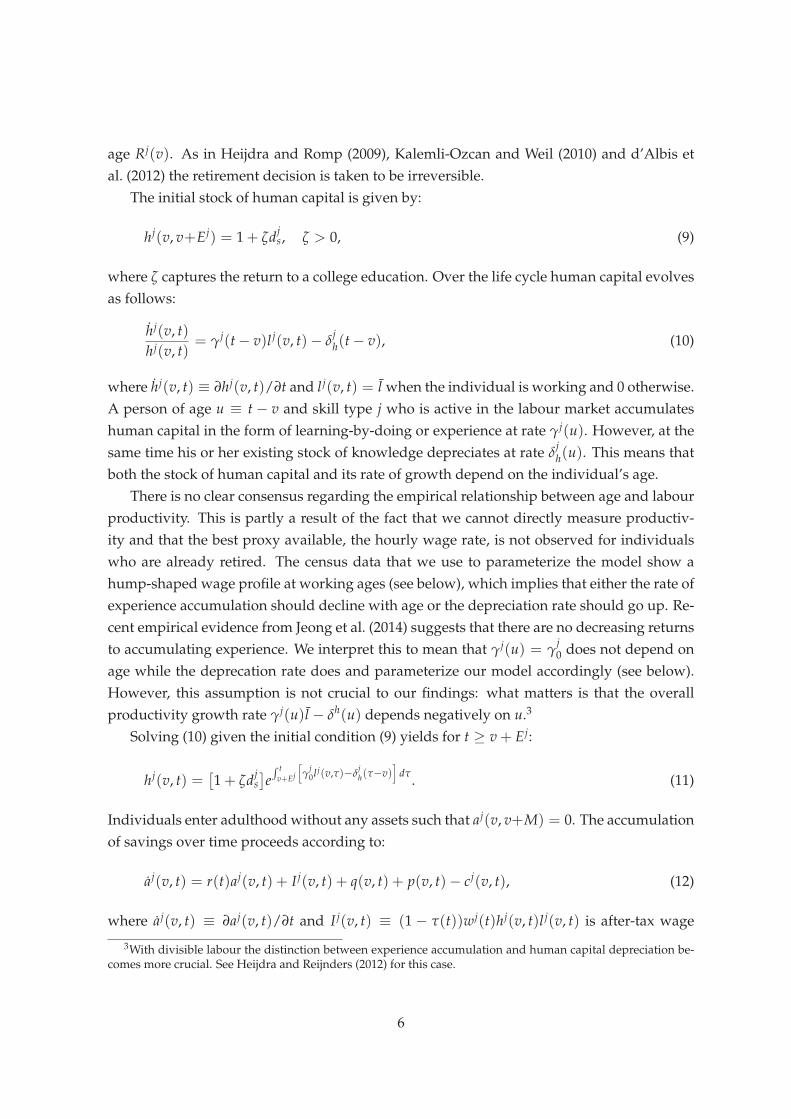
The initial stock of human capital is given by:
hj(v, v+Ej) = 1 + ζdjs, ζ > 0, (9)
where ζ captures the return to a college education. Over the life cycle human capital evolves
as follows:
hj(v, t)
hj(v, t)= γj(t − v)l j(v, t)− δ
jh(t − v), (10)
where hj(v, t) ≡ ∂hj(v, t)/∂t and l j(v, t) = l when the individual is working and 0 otherwise.
A person of age u ≡ t − v and skill type j who is active in the labour market accumulates
human capital in the form of learning-by-doing or experience at rate γj(u). However, at the
same time his or her existing stock of knowledge depreciates at rate δjh(u). This means that
both the stock of human capital and its rate of growth depend on the individual’s age.
There is no clear consensus regarding the empirical relationship between age and labour
productivity. This is partly a result of the fact that we cannot directly measure productiv-
ity and that the best proxy available, the hourly wage rate, is not observed for individuals
who are already retired. The census data that we use to parameterize the model show a
hump-shaped wage profile at working ages (see below), which implies that either the rate of
experience accumulation should decline with age or the depreciation rate should go up. Re-
cent empirical evidence from Jeong et al. (2014) suggests that there are no decreasing returns
to accumulating experience. We interpret this to mean that γj(u) = γj0 does not depend on
age while the deprecation rate does and parameterize our model accordingly (see below).
However, this assumption is not crucial to our findings: what matters is that the overall
productivity growth rate γj(u)l − δh(u) depends negatively on u.3
Solving (10) given the initial condition (9) yields for t ≥ v + Ej:
hj(v, t) =[
1 + ζdjs
]
e∫ t
v+Ej
[
γj0l j(v,τ)−δ
jh(τ−v)
]
dτ. (11)
Individuals enter adulthood without any assets such that aj(v, v+M) = 0. The accumulation
of savings over time proceeds according to:
aj(v, t) = r(t)aj(v, t) + I j(v, t) + q(v, t) + p(v, t)− cj(v, t), (12)
where aj(v, t) ≡ ∂aj(v, t)/∂t and I j(v, t) ≡ (1 − τ(t))wj(t)hj(v, t)l j(v, t) is after-tax wage
3With divisible labour the distinction between experience accumulation and human capital depreciation be-comes more crucial. See Heijdra and Reijnders (2012) for this case.
6

income earned at time t. There is a proportional labour tax τ(t) which is used to finance
pension payments p(v, t) to eligible individuals. We assume that there are no annuities or
life-insured loans available so that the return on financial assets is the real rate of interest.4
The assets left behind by individuals who pass away are redistributed to those who are still
alive in the form of accidental bequests q(v, t). If there is uncertainty about whether a person
might die and there is no life insurance available then individuals cannot borrow money for
fear that they will default on their loan. In order to allow people to borrow funds to finance
their education we assume that survival is certain up to age F > M.5 For the remainder of
life there is a borrowing constraint such that aj(v, t) ≥ 0.
An individual of a given skill type has to determine the level of consumption at each
moment in time cj(v, t) and the age at retirement Rj(v) so as to maximize expected life-time
utility (7) given the process of human capital accumulation (10) and the budget identity
(12). Assuming that the borrowing constraint does not bind, the first-order condition for
consumption can be written as:
1
cj(v, t)e−ρ[t−v−M]S(M, t − v) = λj(v)e−
∫ tv+M r(τ)dτ. (13)
At any given moment in time, the marginal utility of consumption (left-hand side) should
equal the corresponding marginal cost in terms of reduced life-time wealth (right-hand side)
with λj(v) its shadow price.
The first-order condition for the retirement age is given by:
−χ(1 − l)1−σ − 1
1 − σe−ρ[Rj(v)−M]S(M, Rj(v)) = λj(v)I j(v, v+Rj(v))e−
∫ v+Rj(v)v+M r(τ) dτ. (14)
The left-hand side is the increased felicity from leisure while the right-hand side captures
the utility cost of foregone earnings. We discuss the retirement decision in more detail in
Section 3 below.
Finally, each individual has to decide whether or not to become skilled. In doing so
he or she weighs the costs against the benefits. The costs of an education are threefold.
First, leisure during schooling years is reduced by the time required for studying. Second,
the individual has to postpone entry into the labour market and therefore loses potential
wage income. Third, there is a ‘psychic’ or effort cost of studying equal to θ. The benefit
of an education is that it increases human capital and thereby the return to labour. As the
cost is increasing in θ while the benefit is independent of it, the optimal education choice
is governed by a threshold rule. See the upper panel of Figure 2. For a cohort born at
time v there is a value θ(v) such that all individuals for whom θ ≤ θ(v) will decide to
4In reality these kind of financial products do exist, but are not used to a great extent. See for example Cannonand Tonks (2008).
5Since the survival profile is very flat initially this is not a strong assumption.
7

obtain a college degree while all individuals with θ > θ(v) remain uneducated. It follows
that the fraction of skilled individuals in this cohort equals π(v) = Fθ(θ(v)) where Fθ is
the cumulative distribution function of the utility cost of education, see the lower panel of
Figure 2.
2.2.1 Demography and aggregation
At a given time t, the size of the cohort of vintage v is denoted by P(v, t). Over time cohort
members pass away so that:
P(v, t) =
P(v, v)S(0, t − v) for 0 ≤ t − v ≤ D
0 for t − v > D(15)
The size of the total population P(t) =∫ t
t−D P(v, t) dv is found by summing over all living
cohorts. We assume that the economy is in a demographic steady state in which the crude
birth rate b = P(t, t)/P(t) and the population growth rate nP = P(t)/P(t) are constant. This
gives rise to the following equilibrium condition:6
b =1
∆(0, D, nP), (16)
where ∆ is the ‘demographic function’:
∆(u1, u2, ξ) =∫ u2
u1
e−ξ[u−u1]S(u1, u2) du. (17)
In Appendix B we show that the demographic function is strictly positive, decreasing in ξ
and u1 and increasing in u2.
Given the demographic structure of the population we can calculate aggregate values of
effective labour, consumption and financial assets by skill type:
Cj(t) =∫ t−M
t−Dcj(v, t)Pj(v, t) dv,
Lj(t) =∫ t−M
t−Dhj(v, t)l j(v, t)Pj(v, t) dv,
Aj(t) =∫ t−M
t−Daj(v, t)Pj(v, t) dv,
where Ps(v, t) = π(v)P(v, t) is the fraction of skilled individuals in a given cohort and
6By definition of the total population, the birth rate and the population growth rate:
P(t) =∫ t
t−DP(v, t) dv =
∫ t
t−DbP(v)S(0, t − v) dv = bP(t)
∫ D
0e−nPuS(0, u) du = bP(t)∆(0, D, nP)
8

Figure 2: Optimal choice of education
θ
benefit
cost
θθ(v)
Fθ(θ)
π(v)
9

Pu(v, t) = [1 − π(v)]P(v, t) is the fraction of unskilled. It follows that total consumption
and financial assets are given by C(t) = Cu(t) + Cs(t) and A(t) = Au(t) + As(t), respec-
tively.
2.3 Accidental bequests
In the absence of life insurance individuals will pass away with a positive stock of financial
wealth. The way in which these accidental bequests are distributed among survivors has
nontrivial general equilibrium repercussions, see Heijdra et al. (2014). We take a conservative
stance and assume that every adult receives the same amount so that q(v, t) = q(t). The
balanced budget condition then becomes:
∫ t−M
t−Dµ(t − v)
[
au(v, t)Pu(v, t) + as(v, t)Ps(v, t)]
dv = q(t)∫ t−M
t−DP(v, t) dv, (18)
where µ(u) is the mortality rate at age u:
µ(u) ≡ −∂S(u1, u)/∂u
S(u1, u). (19)
Total assets left behind (left-hand side) should equal total bequests (right-hand side).
2.4 Pensions
We introduce a stylized Pay-As-You-Go (PAYG) pension system that provides a benefit to
every person over the age of R (the statutory retirement age) so that p(v, t) = p(t) for t− v ≥
R and zero otherwise. The system is unfunded in the sense that there are no assets but
instead benefits are paid out of current contributions by workers:
τ(t)[
wu(t)Lu(t) + ws(t)Ls(t)]
= p(t)∫ t−R
t−DP(v, t) dv. (20)
Note that we assume that every elderly individual receives the pension benefit regardless of
whether he or she is still working. In this way we prevent large distortions of the retirement
decision. In contrast, real-life pension system might provide strong incentives for retirement
at or close to the statutory age (see for example Heijdra and Romp (2009)).
2.5 Macroeconomic equilibrium
We restrict attention to the long-run equilibrium of the model. A macroeconomic steady
state or balanced growth path is a sequence of prices and allocations such that:
(i) Individuals maximize expected life-time utility taking prices as given.
10

(ii) Firms maximize profits taking prices as given.
(iii) All markets clear.
– Capital market:
K(t) = A(t)
– Goods market:
Y(t) = C(t) + I(t)
– Labour market:
Nu(t) = Lu(t), Ns(t) = Ls(t)
(iv) All variables grow at a constant rate, possibly zero.
Our choice of the utility function ensures that the balanced growth path exists, see King et
al. (2002). In the steady state the share of skilled workers is the same across cohorts and so is
the optimal retirement age for each skill type. Total output, consumption and savings grow
at rate nZ + nP, effective labour grows at rate nP, wages, pensions and bequests grow at rate
nZ and the interest rate is constant over time.
3 The optimal retirement age
When studying the general equilibrium effects of a longevity shock below, changes in the
retirement age play an important role. Therefore we discuss in some more detail how the
optimal (steady-state) retirement age is determined in the model.
By using (13) in (14) we find that the optimal retirement age R∗ has to satisfy:7
−χ(1 − l)1−σ − 1
1 − σ1/cj(v, v+R∗)
= I j(v, v+R∗). (21)
Recall that there is only a labour supply decision at the extensive margin: an individual
works either 0 or l hours. Under this assumption, the left-hand side of (21) can be seen as
7Alternatively we can write:
1
cj(v, v+R∗)I j(v, v + R∗) = −χ
(1 − l)1−σ − 1
1 − σ,
such that the marginal utility of earning a wage should equal the cost of supplying labour. This is similar toequation (11) in d’Albis et al. (2012) or equation (2) in Prettner and Canning (2014).
11
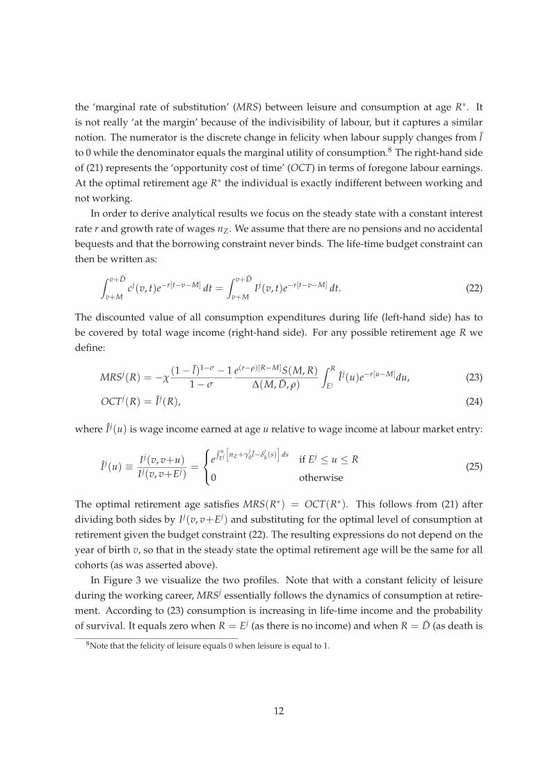
the ‘marginal rate of substitution’ (MRS) between leisure and consumption at age R∗. It
is not really ‘at the margin’ because of the indivisibility of labour, but it captures a similar
notion. The numerator is the discrete change in felicity when labour supply changes from l
to 0 while the denominator equals the marginal utility of consumption.8 The right-hand side
of (21) represents the ‘opportunity cost of time’ (OCT) in terms of foregone labour earnings.
At the optimal retirement age R∗ the individual is exactly indifferent between working and
not working.
In order to derive analytical results we focus on the steady state with a constant interest
rate r and growth rate of wages nZ. We assume that there are no pensions and no accidental
bequests and that the borrowing constraint never binds. The life-time budget constraint can
then be written as:
∫ v+D
v+Mcj(v, t)e−r[t−v−M] dt =
∫ v+D
v+MI j(v, t)e−r[t−v−M] dt. (22)
The discounted value of all consumption expenditures during life (left-hand side) has to
be covered by total wage income (right-hand side). For any possible retirement age R we
define:
MRSj(R) = −χ(1 − l)1−σ − 1
1 − σ
e(r−ρ)[R−M]S(M, R)
∆(M, D, ρ)
∫ R
EjI j(u)e−r[u−M]du, (23)
OCTj(R) = I j(R), (24)
where I j(u) is wage income earned at age u relative to wage income at labour market entry:
I j(u) ≡I j(v, v+u)
I j(v, v+Ej)=
e∫ u
Ej
[
nZ+γj0 l−δ
jh(s)
]
dsif Ej ≤ u ≤ R
0 otherwise(25)
The optimal retirement age satisfies MRS(R∗) = OCT(R∗). This follows from (21) after
dividing both sides by I j(v, v+Ej) and substituting for the optimal level of consumption at
retirement given the budget constraint (22). The resulting expressions do not depend on the
year of birth v, so that in the steady state the optimal retirement age will be the same for all
cohorts (as was asserted above).
In Figure 3 we visualize the two profiles. Note that with a constant felicity of leisure
during the working career, MRSj essentially follows the dynamics of consumption at retire-
ment. According to (23) consumption is increasing in life-time income and the probability
of survival. It equals zero when R = Ej (as there is no income) and when R = D (as death is
8Note that the felicity of leisure equals 0 when leisure is equal to 1.
12

Figure 3: Optimal retirement age
retirement ageEj D
MRSj
OCTj
R∗
certain). The first derivative satisfies:
∂MRSj(R)
∂R=
[
r − ρ − µ(R) +I j(R)e−r[R−M]
∫ REj I j(u)e−r[u−M] du
]
MRSj(R). (26)
At young ages the increase in labour earnings following an extension of the work career
dominates the decrease in the probability of survival so that consumption at retirement goes
up. At older ages this reverses and the expression in (26) becomes negative.
The OCTj profile mimics the hump-shaped pattern of wages over the life cycle. It satis-
fies:
∂OCTj(R)
∂R=
[
nZ + γj0 l − δ
jh(R)
]
OCTj(R), (27)
where δjh(R) is increasing in R. The opportunity cost of time is normalized to unity when
R = Ej and is non-negative for R = D.
As long as the opportunity cost of time exceeds the marginal rate of substitution between
leisure and consumption the individual keeps working. The point of intersection between
the two profiles determines the optimal retirement age. The following proposition describes
how the retirement age is affected by a change in longevity, human capital depreciation or
factor prices.
13
Proposition 1 (Comparative static effects on the retirement age). Suppose that there are no
pensions and bequests and that the borrowing constraint never binds. Assume that there is an interior
solution for the optimal retirement age in the steady state. Keeping everything else constant we have
that for both skill types:
(i) An increase in the survival probabilities has an ambiguous effect on the retirement age.
(ii) A decrease in the depreciation rate has an ambiguous effect on the retirement age.
(iii) An increase in the interest rate leads to a decrease in the retirement age.
(iv) An increase in the wage rate does not affect the retirement age.
Proof. See Appendix A.
In general we cannot say whether an improvement in the probability of survival prompts
individuals to retire earlier or later. Note that in this case only the MRSj profile is affected
and not the OCTj curve. For any possible retirement age there is a positive effect on the
level of consumption at that age due to the increased chances of being alive, but there is
also a negative effect as financial resources have to be spread over a longer (expected) life
time. In the special case that mortality is unchanged at working ages but drops for elderly
individuals, only the latter effect is present so that consumption decreases and retirement is
postponed.9 For example, suppose that S(0, u) = 1 for u ≤ D and S(0, u) = 0 for u > D so
that there is no mortality risk but a certain length of life. An increase in D would then result
in an increase in the retirement age.
In contrast to a longevity boost, a decrease in human capital depreciation at all ages af-
fects both profiles. During the working career human capital is higher at any age so that
there is an increase in the level of wealth (and thereby consumption) as well as the oppor-
tunity cost of time. As a result the effect on the retirement age is again ambiguous. Note,
however, that a change in the depreciation rate at a certain age affects the level of human
capital in the future but not the past. Hence, if improvements in productivity only occur in
old age then the retirement age remains unchanged.
A change in the interest rate influences the price of consumption and leisure at different
points in time and thereby has both an income and substitution effect on the optimal length
of the retirement period (which can be seen as the purchase of leisure). In addition it deter-
mines the extent to which future income is discounted in life-time wealth. The overall effect
is such that a higher interest rate leads to earlier retirement.
The fact that changes in the wage rate do not influence the retirement decision is a con-
sequence of the fact that the utility function satisfies the King-Plosser-Rebelo conditions (see
9A similar result is proved for a more general utility function by d’Albis et al. (2012) for the case that thereis an annuity market (either perfect or imperfect). Cervelatti and Sunde (2011) show that the age profile ofmortality decline also matters for the optimal schooling decision.
14

King et al. (2002)). These ensure that the income and substitution effect of a proportional
wage change on labour supply exactly cancel out. This is necessary for a steady state with
positive wage growth and a constant retirement age to exist.
4 Parameterization
In the next section we will study the long-run effect of a longevity shock on individual
choices and macroeconomic outcomes. As it is not possible to solve for the equilibrium
of the model in closed form we will complement the analytical insights from the previous
section with a simple quantitative exercise. To that end we choose plausible values for the
demographic and economic parameters in line with the United States in the year 2010.
4.1 Demographic parameters
We set the age of majority equal to M = 18. For the survival function we use the functional
form suggested by Boucekkine et al. (2002) but extend it to the case that there is certain
survival up to age F:
S(u1, u2) =
1 for u2 < F
η0 − eη1 max{u2−F,0}
η0 − eη1 max{u1−F,0}for F ≤ u2 < D
0 for u2 ≥ D
η0 > 1, η1 > 0, (28)
where u1 < u2 and D ≡ ln η0/η1. The corresponding life expectancy at birth is given by:
E[D] =∫ D
0S(0, u) du = F +
1
η1
[
η0 ln η0
η0 − 1− 1
]
. (29)
The data on survival probabilities comes from the Office of the Chief Actuary of the Social
Security Administration (SSA) and is described in Bell and Miller (2005). We use the period
life table for males for 2010. Given that the survival function is very flat and close to 1 up
to middle age (see Figure 1 in the introduction) we set F = 45. We divide the number of
individuals who are alive at a given age by the corresponding number at age 45 in order to
obtain the data profile in Figure 4. The parameters η0 and η1 are estimated using nonlinear
least squares, see Table 1. The corresponding maximum age is D = 91.906 while the expected
length of life is 77.489 years.
According to the World Bank the crude birth rate for the United States in 2010 is 14
births per 1000 population. The demographic equilibrium condition (16) then implies that
the population growth rate is 0.209%.
15
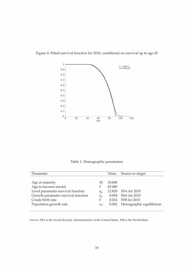
Figure 4: Fitted survival function for 2010, conditional on survival up to age 45
age
0
0.1
0.2
0.3
0.4
0.5
0.6
0.7
0.8
0.9
1
0 20 40 60 80 100 120
datafitted
Table 1: Demographic parameters
Parameter Value Source or target
Age at majority M 18.000Age to become mortal F 45.000Level parameter survival function η0 12.829 SSA for 2010Growth parameter survival function η1 0.054 SSA for 2010Crude birth rate b 0.014 WB for 2010Population growth rate nP 0.002 Demographic equilibrium
Sources: SSA is the Social Security Administration of the United States. WB is the World Bank.
16

4.2 Economic parameters
Even though we do not attempt a full-blown calibration exercise we nevertheless wish to
choose the economic parameters of the model in such a way that they are in line with em-
pirical evidence.
In order to obtain life-cycle profiles for hours worked and the hourly wage earned we
follow an approach similar to Wallenius (2011). We use data from the Current Population
Survey (CPS) for the United States in the years 1976 up to and including 2012. The sample is
restricted to males that work a positive number of hours, have at least a high school diploma
and are between the age of 25 and 55. The reason for restricting attention to this age range
is to avoid sample selection issues as a consequence of schooling and early retirement. For
each individual we have data on the birth year, weeks worked last year, usual hours worked
per week, wage and salary income and educational attainment. We construct pseudo panel
data or synthetic cohorts by following the different representative samples of individuals
with the same year of birth over time. A distinction is made between two skill types: those
with at least 4 years of college (the ‘skilled’) and those with less (the ‘unskilled’).
We normalize hours worked to a unit time endowment under the assumption that in-
dividuals have 14 hours available for work per day or 98 per week. For a given cohort we
find the average number of hours worked at each age by averaging over the corresponding
observations using the sampling weights. We then take the average over cohorts by age and
skill type, see Figure 5(a). The hours profile is nearly flat between ages 25 and 55 for both
skill types, which fits well with our assumption of a labour supply decision at the exten-
sive margin only. We set the time requirement of a full time job equal to the average value
l = 0.440.
We adjust the hourly wages by the consumer price index so that they are measured in
1999 US dollars and comparable across years. For each cohort we find the average hourly
wage at each age by skill type. We then normalize the resulting cohort profiles by the wage at
age 25 of the unskilled. After averaging over cohorts we obtain the life-cycle profile depicted
in Figure 5(b). There is a clear hump-shaped pattern for both skill types.
The parameterization then proceeds as follows. We fix the interest rate at 3.5% per year
and assume that unskilled and skilled individuals earn the same return per unit of effective
labour which is normalized to unity. The long-run economic growth rate is 2%. We set the
rate of time preference equal to ρ = 0.010 and choose a value for the curvature parameter
for the felicity of leisure σ = 2 such that the Frisch labour supply elasticity is about 0.6. The
statutory retirement age is 65 and the tax rate on wage income used to finance the pension
system is equal to 10.6%, which corresponds to the combined contributions of employers
and employees for the US Old Age and Survivors Insurance from 2000 onwards.
We parameterize the experience accumulation and human capital depreciation functions
17

Figure 5: Data profiles and model fit
(a) Hours worked (b) Hourly wage
age
0
0.1
0.2
0.3
0.4
0.5
0.6
0.7
20 30 40 50 60 70 80 90
unskilled, dataskilled, data
age
0
0.5
1
1.5
2
2.5
20 30 40 50 60 70 80 90
unskilled, dataskilled, dataunskilled, modelskilled, model
Source: Current Population Survey for the United States, 1976-2012.
in the following way:
γj(u) = γj0, γ
j0 > 0,
δjh(u) = δ0eδ1 max{u−X,0}, δ0 > 0, δ1 ≥ 0, X ≥ M.
This is similar to Wallenius (2011) but with an age effect in depreciation rather than in ex-
perience for reasons alluded to above. By assuming that the depreciation parameters are
independent of skill type we have chosen parsimony over degrees of freedom in our data
fitting (as described below). Note that if X > M then the depreciation rate is constant at δ0
for young individuals.
For a given set of human capital technology parameters {γu0 , γs
0, δ0, δ1, X, ζ} we iterate
over the life-cycle profiles of both skill types until the pension payment and accidental be-
quests satisfy their respective balanced budget conditions. In every round we update the
preference parameter χ in such a way that the optimal retirement age for an unskilled indi-
vidual is equal to 65. We then calculate the squared relative deviation of the simulated wage
profiles from the empirical values at ages 25, 35, 45 and 55. We choose the set of parameter
values that minimizes this distance.
The resulting profiles are depicted in Figure 5(b) and match the data quite closely. The
parameter estimates in Table 2 show that the return to labour market experience is somewhat
higher for skilled individuals and that having a college education increases start-up human
capital by about 32%. On average a skilled person between ages 25 and 60 earns 52.77%
more per hour than an unskilled individual. The skill premium is somewhat lower than that
18

usually reported. Heathcote et al. (2010), for example, calculate a premium of 90% for males
in 2005. This discrepancy arises because (i) we have excluded individuals with less than a
high school diploma from our sample and (ii) the wage profiles are averages over 37 years
during which time the premium has risen.
Next we calculate the steady-state education threshold and set the location parameter of
the log-normal utility cost distribution in such a way that the fraction of educated individu-
als is 38% (in line with the CPS data) under the assumption that the scale parameter equals
1.10
Finally we set the technology parameters for the firms. The income share of capital φ
is one third and the elasticity of substitution between skilled and unskilled labour is 1.41
as estimated by Katz and Murphy (1992). The remaining parameters are chosen so that the
factor prices are indeed equal to their postulated values.
4.3 Visualization of the benchmark
Some key indicators of the parameterized benchmark equilibrium (BM hereafter) are re-
ported in first column of Table 4 below. The ratio of consumption to output is 0.702, while
the capital-output ratio is 2.435. Both are plausible values.
The steady-state life-cycle profiles for consumption and savings are given in Figure 6.
These are scaled by the level of technology at the age of majority Z(v+ M) to ensure that they
are the same for all cohorts. As long as the borrowing constraint does not bind, consumption
grows at an exponential rate r − ρ − µ(u). This rate is initially positive (when mortality is
low) but becomes negative later in life (when the risk of dying increases). As a consequence
the consumption profile is hump-shaped and reaches a peak around age 70 for both skill
types. As skilled individuals cannot work during their education period they have to borrow
money at the start of life. These loans are fully repaid by the age of 35, well before survival
becomes uncertain.
Ideally individuals would like to let their consumption decrease to zero as they get close
to the maximum age and their chances of survival dwindle. As they still receive income
in the form of pension benefits and accidental bequests this would imply that it is optimal
to borrow money towards the end of life and repay it in the last few years (conditional on
survival). Given that this is not possible, the borrowing constraint will bind and individ-
uals consume exactly their transfer income in each year (which grows at a rate nZ).11 This
explains the upward sloping part of the consumption profile at the end of life for both skill
types. The age at which the constraint starts to bind is such that there is no jump in con-
sumption.
10We have two parameters available (µθ and σθ) to match only one target (the fraction of skilled individuals).We have tried different values of σθ but this does not qualitatively change our results.
11This result is in line with Leung (1994) who shows that if individuals have no bequest motive and annuitymarkets do not exist, then savings must be depleted some time before the maximum lifetime.
19

Table 2: Economic parameters
Parameter Value Source or target
PreferencesPure rate of time preference ρ 0.010Curvature parameter for leisure σ 2.000Preference parameter for leisure χ 0.446 Retirement age unskilled
ProductionIncome share of capital φ 0.330Constant in production function Φ 1.549 Rental ratesDepreciation of physical capital δK 0.101 Interest rateEconomic growth rate nZ 0.020Substitution elasticity between skill types ψ 1.410 Katz and Murphy (1992)Time requirement of a full-time job l 0.440 Average hours CPSWeight of unskilled labour in composite β 0.529 Equal marginal products
GovernmentPension tax rate τ 0.106 SSA for 2010Statutory retirement age R 65.000
Human capitalExperience parameter for unskilled γu
0 0.094 Wage profiles CPSExperience parameter for skilled γs
0 0.117 Wage profiles CPSLevel parameter depreciation profile δ0 0.022 Wage profiles CPSGrowth parameter depreciation profile δ1 0.040 Wage profiles CPSAge after which depreciation increases X 18.000 Wage profiles CPS
EducationReturn to education ζ 0.321 Wage profiles CPSLocation parameter talent distribution µθ 2.641 Fraction educated CPSScale parameter talent distribution σθ 1.000Time requirement of a college education e 0.400
Sources: SSA is the Social Security Administration of the United States. CPS is the Current Population Survey of
the United States.
20

In Table 4 we see that skilled individuals retire from the labour force just before reaching
age 70, which is almost 5 years later than the unskilled. The second bump in their asset
profile (see the dashed line in Figure 6(b)) is a consequence of the fact that they start to
receive their pension payments while they are still working.
Figure 6: Steady-state life-cycle profiles in the benchmark
(a) Consumption (b) Financial assets
age
0.4
0.5
0.6
0.7
0.8
0.9
1
1.1
1.2
1.3
20 30 40 50 60 70 80 90
unskilledskilled
age
−2
−1
0
1
2
3
4
5
6
7
20 30 40 50 60 70 80 90
unskilledskilled
5 The long-run effects of increased longevity
In this section we show the long-run effects predicted by the model of two stylized longevity
shocks. The first is a biological longevity boost (BLB), which consists of an outward shift of the
survival function. Secondly we consider what happens if this increase in the expected length
of life is accompanied by an improvement in labour productivity at all ages, this is referred
to as the comprehensive longevity boost (CLB).
5.1 Biological longevity boost
If the survival function shifts outward in the way forecasted by the SSA for 2100 (see Figure
1 in the introduction), then the demographic equilibrium changes. We estimate a new set of
parameters to fit the data profile for 2100 conditional on survival up to age 45. The maximum
age increases to D = 96.968 and life expectancy at birth goes up by more than 6 years to
83.638, see Table 3. As the population growth rate is unaffected (under the assumption that
nothing has happened to fertility) the crude birth rate will have to fall. In panel (a) of Figure
7 we see that the inverse of the demographic function shifts down which for a given nP leads
to a lower b.
21
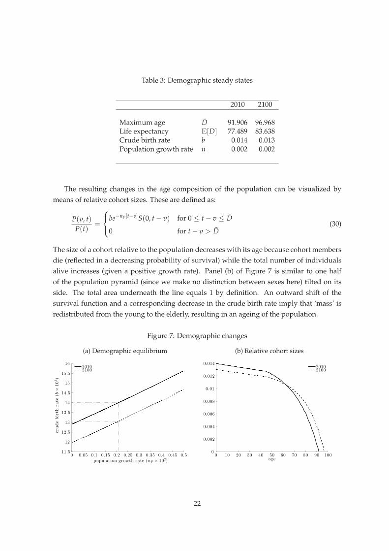
Table 3: Demographic steady states
2010 2100
Maximum age D 91.906 96.968Life expectancy E[D] 77.489 83.638Crude birth rate b 0.014 0.013Population growth rate n 0.002 0.002
The resulting changes in the age composition of the population can be visualized by
means of relative cohort sizes. These are defined as:
P(v, t)
P(t)=
be−nP[t−v]S(0, t − v) for 0 ≤ t − v ≤ D
0 for t − v > D(30)
The size of a cohort relative to the population decreases with its age because cohort members
die (reflected in a decreasing probability of survival) while the total number of individuals
alive increases (given a positive growth rate). Panel (b) of Figure 7 is similar to one half
of the population pyramid (since we make no distinction between sexes here) tilted on its
side. The total area underneath the line equals 1 by definition. An outward shift of the
survival function and a corresponding decrease in the crude birth rate imply that ‘mass’ is
redistributed from the young to the elderly, resulting in an ageing of the population.
Figure 7: Demographic changes
(a) Demographic equilibrium (b) Relative cohort sizes
population growth rate (nP × 102)
crudebirth
rate
(b×
103)
11.5
12
12.5
13
13.5
14
14.5
15
15.5
16
0 0.05 0.1 0.15 0.2 0.25 0.3 0.35 0.4 0.45 0.5
20102100
age
0
0.002
0.004
0.006
0.008
0.01
0.012
0.014
0 10 20 30 40 50 60 70 80 90 100
20102100
22

The quantitative long-run consequences of a biological longevity boost are summarized
in Table 4. Initially we assume that the statutory retirement age and the pension benefit re-
main fixed and that the tax rate adjusts to balance the budget of the pension system as given
in (20). This is known as a Defined Benefit (DB) pension. Keeping factor prices constant at
their values in the benchmark, the first column under the BLB heading reports the partial
equilibrium effects of the longevity shock. The retirement age decreases a little for both skill
types, which means that individuals expect to spend a significantly longer part of their life
in retirement. As a consequence the pension tax rate has to increase from 10.6% to 14.5%.
The fraction of educated individuals goes up by almost 2 percentage points as the increased
probability of survival during working ages raises the expected payoff of a college degree.
We wish to make two remarks regarding these partial equilibrium results. First, it would
be misleading to interpret the findings as pertaining to a small open economy. For such
an economy the factor prices are determined in the rest of the world, but as most countries
experience very similar demographic changes these prices cannot be expected to remain
constant. Second, the extent to which the fraction of skilled individuals changes depends
crucially on the dispersion of educational talent in the population. For a given shift in the
education threshold, a lower (higher) value of the scale parameter σθ of the utility cost dis-
tribution would have increased (decreased) the proportion of educated individuals relative
to that reported in Table 4.12 However, qualitatively the results remains the same: it is more
attractive to get a college degree.
The next column gives the general equilibrium outcomes under the DB system. Indi-
viduals have to save more in order to finance their extended retirement period, which leads
to an increase in the capital intensity of production. This results in a drop in the return to
capital and a rise in the unit cost of effective labour. The latter has no effect on the retirement
decision but the lower interest rate induces an increase in the retirement age, see Proposition
1. The change in the skill distribution lowers the rental rate on skilled relative to unskilled
effective labour. This reduces the incentive to obtain an education and therefore the general
equilibrium effect on the fraction of skilled individuals is smaller than the partial equilib-
rium effect (although still positive).
In the final two columns under the BLB heading we explore alternative assumptions re-
garding the closure rule for the pension system. The first is a Defined Contribution (DC)
system whereby the tax rate on wage income remains constant while the pension benefit ad-
justs to balance the budget. Compared to the DB case individuals work about a year longer
and save more for old age which results in a further increase in the capital intensity and
reduction of the interest rate. The second possibility is to keep both the tax rate and benefit
constant and instead change the Statutory Age (SA) for retirement. In terms of macroeco-
nomic outcomes this scenario is in between the previous two. The age at which individuals
12The variance of the log-normal distribution is given by (eσ2θ − 1)e2µθ+σ2
θ which is increasing in σθ .
23

Table 4: Quantitative results
BM BLB CLBPE DB DC SA PE DB DC SA
IndividualsFraction skilled (in %p) 38.000 39.685 38.619 39.170 39.138 46.907 38.707 38.834 38.882Retirement age unskilled 65.000 64.593 65.573 66.700 66.588 70.578 70.349 70.632 70.571Retirement age skilled 69.468 68.893 69.696 70.674 70.534 75.226 74.942 75.192 75.130
FirmsCapital intensity 7.251 7.559 7.845 7.781 7.183 7.238 7.218Skilled to unskilled labour 0.849 0.874 0.893 0.892 0.918 0.922 0.922
Factor pricesInterest rate (in %p) 3.500 3.127 2.803 2.874 3.586 3.517 3.542Unit cost effective labour 1.995 2.023 2.048 2.042 1.989 1.994 1.992Rental rate unskilled 1.000 1.024 1.043 1.040 1.023 1.027 1.026Rental rate skilled 1.000 1.003 1.007 1.004 0.968 0.968 0.967
Pension systemStatutory retirement age 65.000 65.000 65.000 65.000 70.301 65.000 65.000 65.000 66.535Pension tax rate (in %p) 10.600 14.536 14.312 10.600 10.600 11.067 11.474 10.600 10.600Pension payment 0.180 0.180 0.180 0.136 0.180 0.180 0.180 0.167 0.180
WelfareEquivalent variation (in %) 5.324 6.744 3.224 2.264
24

become eligible for pension benefits goes up by 5.30 years, about 1 year less than the increase
in the expected life span. Unskilled individuals choose to retire from the labour force almost
4 years before the pension payments start.
We can compare the three different pension systems in terms of their effect on steady state
welfare. In particular, we calculate the percentage by which consumption should change at
each moment in time under the DB system in order to make an individual as well off as
under one of the alternative pension schemes (an equivalent variation exercise). For each
level of the utility cost of education θ we find ω(v|θ) as the solution to:
max{
ΛuDB(v|θ), Λ
sDB(v|θ)
}
+ ∆(M, D, ρ) ln(1+ ω(v|θ)) = max{
Λui (v|θ), Λ
si (v|θ)
}
, (31)
where the subscript i ∈ {DB, DC, SA} indicates the type of pension scheme. Note that each
individual chooses to be skilled or unskilled depending on whichever option gives the high-
est expected utility. We can then calculate the average over all different educational ability
types to obtain:
ω(v) =∫
∞
0ω(v|θ) dFθ(θ). (32)
In the steady state this number does not depend on the date of birth v. The last row of Table 4
reports the average value multiplied by 100%. For example, if there is a biological longevity
boost then on average individuals would require 5.32% more consumption under the DB
regime to be as well off as under a Defined Contribution pension scheme and 6.74% to be
indifferent with respect to a system that changes the statutory retirement age. It follows that
the latter is to be preferred in welfare terms under the BLB.
5.2 Comprehensive longevity boost
In case of a comprehensive longevity boost individuals not only expect to live longer but
are also more productive during their working career. Unfortunately we do not have any
data on forecasted productivity changes. Instead we use a parametric approach and model
a productivity improvement as a rightward shift of the human capital depreciation profile
through an increase in the parameter X. Figure 8 shows the original and new depreciation
rates under the assumption that the change in X equals that in life expectancy (about 6 years).
This implies that a person of age 50 now loses skills at the rate that someone of age 44 did
previously, etcetera.
As before, the first column in Table 4 under the CLB heading gives the partial equilib-
rium effect in case of a Defined Benefit pension system. The retirement age increases with
more than 5 years for both skill types and the fraction of skilled individuals rises by about
7 percentage points. Since people are on average more productive and work longer, the
pension tax rate need hardly increase. The general equilibrium repercussions through factor
25
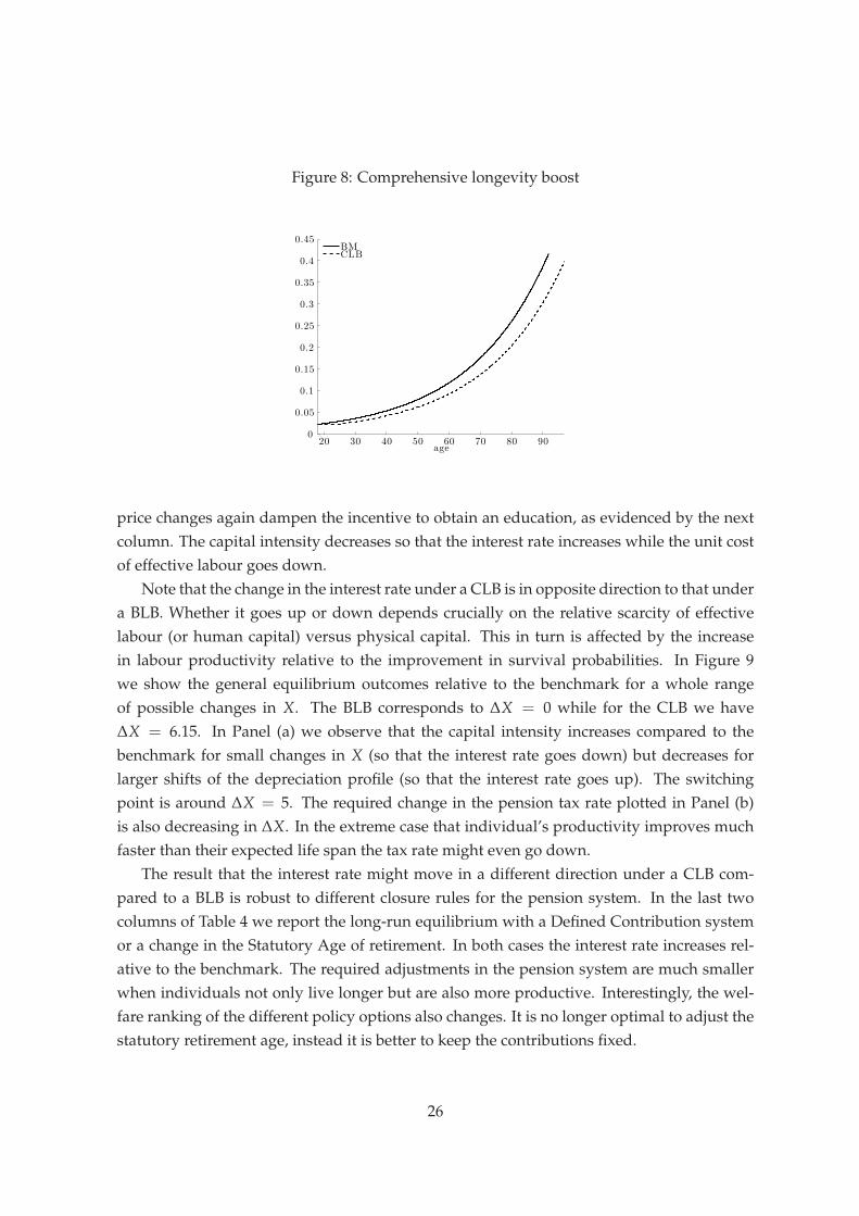
Figure 8: Comprehensive longevity boost
age
0
0.05
0.1
0.15
0.2
0.25
0.3
0.35
0.4
0.45
20 30 40 50 60 70 80 90
BMCLB
price changes again dampen the incentive to obtain an education, as evidenced by the next
column. The capital intensity decreases so that the interest rate increases while the unit cost
of effective labour goes down.
Note that the change in the interest rate under a CLB is in opposite direction to that under
a BLB. Whether it goes up or down depends crucially on the relative scarcity of effective
labour (or human capital) versus physical capital. This in turn is affected by the increase
in labour productivity relative to the improvement in survival probabilities. In Figure 9
we show the general equilibrium outcomes relative to the benchmark for a whole range
of possible changes in X. The BLB corresponds to ∆X = 0 while for the CLB we have
∆X = 6.15. In Panel (a) we observe that the capital intensity increases compared to the
benchmark for small changes in X (so that the interest rate goes down) but decreases for
larger shifts of the depreciation profile (so that the interest rate goes up). The switching
point is around ∆X = 5. The required change in the pension tax rate plotted in Panel (b)
is also decreasing in ∆X. In the extreme case that individual’s productivity improves much
faster than their expected life span the tax rate might even go down.
The result that the interest rate might move in a different direction under a CLB com-
pared to a BLB is robust to different closure rules for the pension system. In the last two
columns of Table 4 we report the long-run equilibrium with a Defined Contribution system
or a change in the Statutory Age of retirement. In both cases the interest rate increases rel-
ative to the benchmark. The required adjustments in the pension system are much smaller
when individuals not only live longer but are also more productive. Interestingly, the wel-
fare ranking of the different policy options also changes. It is no longer optimal to adjust the
statutory retirement age, instead it is better to keep the contributions fixed.
26

Figure 9: General equilibrium outcomes for different values of X
(a) Change in capital intensity (in %) (b) Change in pension tax (in %p)
−5
−4
−3
−2
−1
0
1
2
3
4
5
0 1 2 3 4 5 6 7 8 9 10∆X
−0.04
−0.03
−0.02
−0.01
0
0.01
0.02
0.03
0.04
0 1 2 3 4 5 6 7 8 9 10∆X
6 Conclusion
In this paper we study the long-run effects of a longevity increase on individual decisions
about education and retirement, taking macroeconomic repercussions through endogenous
factor prices and the pension system into account. We build a model of a closed economy in-
habited by overlapping generations of finitely-lived individuals whose labour productivity
depends on their age through the build-up of labour market experience and the deprecia-
tion of human capital. In this context we present analytical results and a simple quantitative
exercise regarding the steady-state effects of two stylized shocks. The first is a biological
longevity boost, which consists of an outward shift of the survival function. We find that
individuals work a little longer but spend most of the additional years in retirement. This
prompts an increase in savings, which raises the capital intensity of production and lowers
the interest rate. The labour tax rate required to finance a Defined Benefit Pay-As-You-Go
pension system increases by almost 3 percentage points. In contrast, if the increase in life
expectancy is accompanied by an improvement in labour productivity through a decrease in
human capital depreciation then the retirement age increases significantly. Under this com-
prehensive longevity boost it is possible that human capital becomes relatively abundant in
production, resulting in a lower unit cost of effective labour and an increase in the interest
rate. As individuals work longer the pension tax rate need hardly change.
References
d’Albis, H., Lau, S.-H. P., and Sanchez-Romero, M. (2012). Mortality transition and differen-
tial incentives for early retirement. Journal of Economic Theory, 147:261–283.
27
Bell, F. C. and Miller, M. L. (2005). Life tables for the United States Social Security Area 1900-
2100. SSA Pub. 11-11536, Social Security Administration, Office of the Chief Actuary.
Boucekkine, R., de la Croix, D., and Licandro, O. (2002). Vintage human capital, demo-
graphic trends, and endogenous growth. Journal of Economic Theory, 104:340–375.
Cannon, E. and Tonks, I. (2008). Annuity Markets. Oxford University Press, Oxford.
Cervellati, M. and Sunde, U. (2013). Life expectancy, schooling, and lifetime labor supply:
Theory and evidence revisited. Econometrica, 81(5):2055–2086.
Heathcote, J., Perri, F., and Violante, G. L. (2010). Unequal we stand: An empirical analysis
of economic inequality in the United States, 1967–2006. Review of Economic Dynamics,
13:15–51.
Heckman, J. J., Lochner, L., and Taber, C. (1998). Explaining rising wage inequality: Explo-
rations with a dynamic general equilibrium model of labor earnings with heterogeneous
agents. Review of Economic Dynamics, 1:1–58.
Heijdra, B. J., Mierau, J. O., and Reijnders, L. S. M. (2014). A tragedy of annuitization?
Longevity insurance in general equilibrium. Macroeconomic Dynamics, 18:1607–1634.
Heijdra, B. J. and Romp, W. E. (2009). Retirement, pensions, and ageing. Journal of Public
Economics, 93:586–604.
Jeong, H., Kim, Y., and Manovskii, I. (2014). The price of experience. Working Paper 20457,
NBER, Cambridge, MA.
Kalemli-Ozcan, S., Ryder, H. E., and Weil, D. N. (2000). Mortality decline, human capital
investment, and economic growth. Journal of Development Economics, 62:1–23.
Kalemli-Ozcan, S. and Weil, D. N. (2010). Mortality change, the uncertainty effect, and re-
tirement. Journal of Economic Growth, 15:65–91.
Katz, L. F. and Murphy, K. M. (1992). Changes in relative wages, 1963-1987: Supply and
demand factors. The Quarterly Journal of Economics, 107(1):35–78.
Keane, M. (2011). Labor supply and taxes: A survey. Journal of Economic Literature, 49(4):961–
1075.
King, M., Ruggles, S., Alexander, J. T., Flood, S., Genadek, K., Schroeder, M. B., Trampe, B.,
and Vick, R. (2010). Integrated Public Use Microdata Series, Current Population Survey:
Version 3.0. machine-readable database, University of Minnesota, Minneapolis.
King, R. G., Plosser, C. I., and Rebelo, S. T. (2002). Production, growth and business cycles:
Technical appendix. Computational Economics, 20:87–116.
28
Leung, S. F. (1994). Uncertain lifetime, the theory of the consumer, and the life cycle hypoth-
esis. Econometrica, 62:1233–1239.
Ludwig, A., Schelkle, T., and Vogel, E. (2012). Demographic change, human capital and
welfare. Review of Economic Dynamics, 15:94–107.
Prettner, K. and Canning, D. (2014). Increasing life expectancy and optimal retirement in
general equilibrium. Economic Theory, 56(1):191–217.
Wallenius, J. (2011). Human capital accumulation and the intertemporal elasticity of substi-
tution of labor: How large is the bias? Review of Economic Dynamics, 14:577–591.
29

A Economic proofs
Proposition 1 (Comparative static effects on the retirement age). Suppose that there are no
pensions and bequests and that the borrowing constraint never binds. Assume that there is an interior
solution for the optimal retirement age in the steady state. Keeping everything else constant we have
that for both skill types:
(i) An increase in the survival probabilities has an ambiguous effect on the retirement age.
(ii) A decrease in the depreciation rate has an ambiguous effect on the retirement age.
(iii) An increase in the interest rate leads to a decrease in the retirement age.
(iv) An increase in the wage rate does not affect the retirement age.
Proof. The optimal retirement age is at the intersection of the following two curves:
MRSj(R) = MUze−(r−ρ)[R−M]S(M, R)
∆(M, D, ρ)
∫ R
EjI j(u)e−r[u−M] du,
OCTj(R) = e∫ R
Ej
[
nZ+γj(s)l−δjh(s)
]
ds,
where MUz is a positive constant:
MUz ≡ −χ(1 − l)1−σ − 1
1 − σ> 0.
We note the following properties of the two curves:
(1) The initial value of OCTj is strictly greater than that of MRSj:
OCT(Ej) = 1 > MRS(Ej) = 0.
(2) The final value of OCTj is at least as large as that of MRSj:
OCT(D) ≥ 0 = MRS(D).
(3) MRSj is initially increasing in R and then decreasing:
∂MRSj(R)
∂R=
[
r − ρ − µ(R) +I j(R)e−r[R−M]
∫ REj I j(u)e−r[u−M] du
]
MRSj(R),
since r > ρ and µ(R) = 0 for R < F but µ(R) → ∞ as R → D.
30

(4) OCTj is initially increasing in R and then decreasing:
∂OCTj(R)
∂R=
[
nZ + γj(R)l − δjh(R)
]
OCTj(R),
since γj(R) is constant while δjh(R) is increasing in R.
Let R∗0 denote the optimal retirement age in the initial steady state equilibrium. We assume
that this is an interior solution so that OCTj(R∗0) = MRSj(R∗
0). The new optimal retirement
age is higher than the initial one if OCTj(R∗0) increases relative to MRSj(R∗
0) and lower oth-
erwise.
(i) Suppose that S(M, u) weakly increases for any given u.
– There is no change in OCTj(R∗0).
– The change in MRSj(R∗0) is ambiguous as ∆(M, D, ρ) increases as well.
It follows that the effect on the retirement age is ambiguous.
(ii) Suppose that δjh(u) weakly decreases for any given u.
– There is an increase in OCTj(R∗0).
– There is an increase in MRSj(R∗0).
It follows that the effect on the retirement age is ambiguous.
(iii) Suppose that r increases.
– There is no change in OCTj(R∗0).
– There is an increase in MRSj(R∗0):
∂MRSj(R∗0)
∂r= MUz
e−ρ[R∗0−M]S(M, R∗
0)
∆(M, D, ρ)
∫ R∗0
Ej[R∗
0 − u] I j(u)er[R∗0−u] du > 0.
It follows that the retirement age decreases.
(iv) Suppose that wj(t) increases.
– There is no change in OCTj(R∗0).
– There is no change in MRSj(R∗0).
It follows that the retirement age remains unchanged.
31

B Demographic proofs
Definition 1 (Demographic function). For |ξ| ≪ ∞ and 0 ≤ u1 < u2 ≤ D the demographic
function is defined as:
∆(u1, u2, ξ) =∫ u2
u1
e−ξ[u−u1]S(u1, u) du.
Note that by integrating (19) the survival function can be written as:
S(u1, u) = e−∫ u
u1µ(s) ds
,
where µ(s) is the mortality rate at age s. We assume that µ(s) = 0 for 0 ≤ s < F and µ(s) > 0
with µ′(s) > 0 and µ′′(s) > 0 for F ≤ s ≤ D.
Lemma 1 (Upper bound). The demographic function has the following upper bound:
∆(u1, u2, ξ) ≤1
ξ + µ(u1).
Proof. Since µ(s) = 0 for 0 ≤ s < F we can write the demographic function as:
∆(u1, u2, ξ) =∫ u
u1
e−ξ[u−u1] du +∫ u2
ue−
∫ u1u [ξ+µ(s)] ds du.
where u = max{u1, min{F, u2}}. We consider three different possibilities.
(1) u1 < u2 ≤ F so that u = u2 and µ(u1) = 0
The demographic function satisfies:
∆(u1, u2, ξ) =∫ u2
u1
e−ξ[u−u1] du =
1 − e−ξ[u2−u1]
ξif ξ 6= 0
u2 − u1 if ξ = 0
In either case the result is less than 1/ξ.
(2) F < u1 < u2 so that u = u1 and µ(u1) > 0
The function MU(u1, u) =∫ u
u1µ(s) ds for u ≥ u1 is a non-negative, increasing and
convex function of u:
MU(u1, u1) = 0,∂MU(u1, u)
∂u= µ(u) ≥ 0,
∂MU2(u1, u)
∂u2= µ′(u) ≥ 0.
32

It follows that:
MU(u1, u) ≥ MU(u1, u1) +∂MU(u1, u1)
∂u[u − u1] = µ(u1)[u − u1].
Hence the demographic function satisfies:
∆(u1, u2, ξ) ≤∫ u2
u1
e−[ξ+µ(u1)][u−u1] du
=
1 − e−[ξ+µ(u1)][u2−u1]
ξ + µ(u1)if ξ + µ(u1) 6= 0
u2 − u1 if ξ + µ(u1) = 0
In either case the result is less than 1/[ξ + µ(u1)].
(3) u1 ≤ F ≤ u2 so that u = F and µ(u1) = 0
The demographic function satisfies:
∆(u1, u2, ξ) = ∆(u1, F, ξ) + e−ξ(F−u1)∆(F, u2, ξ)
≤1 − e−ξ(F−u1)
ξ+
e−ξ(F−u1)
ξ + µ(F)=
1
ξ,
which follows from the results above and the fact that µ(F) ≥ 0.
Proposition 2 (Properties of the demographic function). The demographic function has the fol-
lowing properties:
(i) Positive, ∆(u1, u2, ξ) > 0
(ii) Decreasing in u1, ∂∆(u1, u2, ξ)/∂u1 < 0
(iii) Increasing in u2, ∂∆(u1, u2, ξ)/∂u2 > 0
(iv) Decreasing in ξ, ∂∆(u1, u2, ξ)/∂ξ < 0
Proof. Part (i) is obvious. The first derivatives of the demographic function are:
∂∆(u1, u2, ξ)
∂u1= [ξ + µ(u1)]∆(u1, u2, ξ)− 1,
∂∆(u1, u2, ξ)
∂u2= e−ξ[u2−u1]S(u1, u2),
∂∆(u1, u2, ξ)
∂ξ= −
∫ u2
u1
[u − u1]S(u1, u) du.
Part (iii) and (iv) are straightforward. Part (ii) follows from Lemma 1.
33

C Computational details
C.1 Individual choices
In the steady state the optimal choices only depend on an individual’s age u ≡ t − v, pro-
vided that we scale consumption and financial assets by the level of productivity at age M.
We define:
cj(u) =cj(v, v + u)
Z(v + M), aj(u)=
aj(v, v + u)
Z(v + M),
l j(u) = l j(v, v + u), hj(u) = hj(v, v + u).
We take as given the (constant) level of accidental bequests q ≡ q(t)/Z(t), tax rate on wage
income τ, pension provisions p ≡ p(t)/Z(t), interest rate r and rental rates on effective
labour wj ≡ wj(t)/Z(t) and assume that the borrowing constraint only binds in the final
years of life (we can check this ex post).
(1) For any combination of the retirement age Rj and the age at which the borrowing
constraint starts to bind Rj ≤ Bj ≤ D we can calculate the life-cycle profiles.
– Labour supply:
l j(u) =
0 for M ≤ u < Ej
l for Ej ≤ u < Rj
0 for Rj ≤ u ≤ D
– Human capital:
hj(u) =[
1 + ζdjs
]
e∫ u
Ej
[
γj0 l−δ
jh(s)
]
ds
– Consumption:
cj(u) =
e(r−ρ)[u−M]S(M, u)
∆(M, Bj, ρ)W j(Bj) for M ≤ u < Bj
[
q + p]
enZ [u−M] for Bj ≤ u ≤ D
where W j(Bj) is the discounted value of wage income earned and transfers re-
ceived between ages M and Bj:
W j(Bj) =∫ Bj
MenZ [u−M]
[
(1 − τ)wjhj(u)l j(u) + q + p1u≥R
]
e−r[u−M] du
with 1u≥R the indicator function that equals 1 if u ≥ R and zero otherwise.
34
– Financial assets:
aj(u) =∫ u
MenZ [s−M]
[
(1 − τ)wjhj(s)l j(s) + q + p1s≥R − cj(s)]
e−r[s−u] ds
(2) For any retirement age Rj we can find the optimal Bj by ensuring that at this age there
is no jump in consumption:
e(r−ρ)[Bj−M]S(M, Bj)
∆(M, Bj, ρ)W j(Bj) =
[
q + p]
enZ [Bj−M]
(3) The optimal retirement age Rj is the one that maximizes expected lifetime utility and
is calculated using a minimization routine.
(4) We can find the threshold value for education as the difference between the expected
lifetime utility of a skilled individual (ignoring the utility cost of education) and an
unskilled individual.
C.2 Macroeconomic equilibrium
To calculate the macroeconomic equilibrium we start with a guess for the scaled capital stock
K ≡ K(t)/[Z(t)P(t)] and the two types of effective labour N j ≡ N j(t)/P(t) for j ∈ {u, s}.
Jointly they determine the factor prices wj and r. We find the optimal life-cycle profiles
of skilled and unskilled individuals and the corresponding education threshold. It is then
possible to aggregate across individuals to obtain total consumption C ≡ C(t)/[Z(t)P(t)],
financial assets A ≡ A(t)/[Z(t)P(t)] and effective labour supply L ≡ L(t)/P(t).
We check whether the goods market is in equilibrium so that Y = C + I where Y ≡
Y(t)/[Z(t)P(t)] = ΦKφN1−φ and I ≡ I(t)/[Z(t)P(t)] = (δK + nP + nZ)K. If so, then we
have found the steady state. If not, then we change the level of accidental bequests and one
of the parameters of the pension system using the respective balanced budget conditions. In
addition we partially update the guess for the factor supplies in the direction of satisfying the
capital market equilibrium condition K = A and the labour market equilibrium condition
N = L.
35