Embed Size (px)
Citation preview

The Agglomeration of Bankruptcy∗
Efraim BenmelechKellogg School of Management, Northwestern University and NBER
Nittai BergmanMIT Sloan and NBER
Anna MilanezDeloitte LLP
Vladimir MukharlyamovHarvard University
First Version: May 2012
This Version: September 2015
∗ We thank Douglas Baird, Bo Becker, Shikma Benmelech, John Campbell, Shawn Cole, Jennifer Dlugosz, Richard
Frankel, Jerry Green, Yaniv Grinstein, Barney Hartman-Gleser, Ben Iverson, Steve Kaplan, Prasad Krishnamurthy,
Kai Li (discussant), Anup Malani, David Matsa, Roni Michaely, Ed Morrison, Boris Nikolov (discussant), Randy
Picker, Andrei Shleifer, Matthew Spiegel, David Sraer (discussant), Jeremy Stein and seminar participants at Aalto
University, Adam Smith Workshop for Corporate Finance 2014, City University Hong Kong Finance Conference,
Edinburgh Corporate Finance Conference, The Federal Reserve Bank of Boston, Harvard University, Koc University,
The University of British Columbia, The University of Chicago Law and Economics 2013 seminar, The University
of Chicago Booth School of Business, IDC Herzliya 2013 Summer Conference, Northwestern University (Kellogg),
University of Alberta, UCLA (Anderson), University of Maryland (Smith), University of North Carolina (Kenan-
Flagler), Washington University, Yale School of Management, and Yeshiva University (Syms School of Business)
for very helpful comments. Savita Barrowes, David Choi and Sammy Young provided excellent research assistance.
Benmelech is grateful for financial support from the Guthrie Center for Real Estate Research at the Kellogg School
of Management and from the National Science Foundation under CAREER award SES-0847392. All errors are our
own.
Corresponding author: Efraim Benmelech, Kellogg School of Management, Northwestern University, Sheridan Road
2001, Evanston, IL 60208. E-mail: [email protected].

The Agglomeration of Bankruptcy
Abstract
This paper identifies a new channel through which bankrupt firms impose negative externalities on
non-bankrupt peers. The bankruptcy and liquidation of a retail chain weakens the economies of
agglomeration in any given local area, reducing the attractiveness of retail centers for remaining
stores leading to contagion of financial distress. We find that companies with greater geographic
exposure to bankrupt retailers are more likely to close stores in affected areas. We further show
that the effect of these externalities on non-bankrupt peers is higher when the affected stores are
smaller and are operated by firms with poor financial health.

I. Introduction
How does bankruptcy spread? While research on bankruptcy and financial distress has documented
how bankruptcy reorganizations affect firms that file for Chapter-11 themselves, there is limited
evidence on the effect of bankruptcies and financial distress on competitors and industry peers.
In this paper, we identify a new channel by which bankrupt firms impose negative externalities
on their non-bankrupt competitors, namely, through their impact on peer firm sales and on the
propensity to close stores.
Research in industrial organization has argued that the geographic concentration of stores and
the existence of clusters of stores can be explained by consumers’ imperfect information and their
need to search the market (Wolinsky (1983)). Indeed, both practitioners and academics argue that
economies of agglomeration exist in retail since some stores – those of national name-brands or
anchor department stores, in particular – draw customer traffic not only to their own stores but
also to nearby stores. As a result, store level sales may depend on the sales of neighboring stores for
reasons that are unrelated to local economic conditions (Gould and Pashigian (1998) and Gould,
Pashigian and Prendergast (2005)).
We conjecture that the externalities that exist between neighboring stores, and the economies
of agglomeration they create, can be detrimental during downturns, propagating and amplifying
the negative effects of financial distress and bankruptcies among firms in the same locality. Our
main prediction is that, due to agglomeration economies, retail stores in distress impose negative
externalities on their neighboring peers: store sales tend to decrease with the reduction in sales,
and ultimately the closure, of neighboring stores. If such negative externalities are sufficiently
strong, bankruptcies, and the store closure they involve, will lead to additional store closures and
bankruptcies, propagating within a given area.
Identifying a causal link, however, from the bankruptcy and financial distress of one retailer
to the sales and closure decisions of its neighboring retailers is made difficult by the fact that
bankruptcy filings and financial distress are correlated with local economic conditions. Correlation
in sales among stores in the same vicinity may therefore simply reflect weak demand in an area.
Similarly, the fact that store closures tend to cluster locally may often be the outcome of underlying
difficulties in the local economy, rather than the effect of negative externalities among stores. Local
economic conditions will naturally drive a correlation in outcomes among stores located in the same
1

area.
Using a novel and detailed dataset of all national chain store locations and closures across
the United States from 2005 to 2010, we provide empirical evidence that supports the view that
bankruptcies of retail companies impose negative externalities on neighboring stores owned by sol-
vent companies. Our identification strategy consists of analyzing the effect of Chapter 11 bankrupt-
cies of large national retailers, such as Circuit City and Linens n Things, who liquidated their entire
store chain during the sample period. Using Chapter 11 bankruptcies of national retailers alleviates
the concern that local economic conditions led to the demise of the company: it is unlikely that a
large retail chain will suffer major financial difficulties because of a localized economic downturn in
one of its many locations. Supporting this identification assumption, we show that stores of retail
chains that eventually end up in Chapter 11 bankruptcy are not located in areas that are worse
than the location of stores operated by chains that do not end up in bankruptcy, along a host of
economic characteristics.
We then show that stores located in proximity to stores of national chains that are liquidated
are more likely to close themselves. Importantly, we find that this effect is stronger for stores in the
same industry of the liquidating national chain as compared to stores in industries different from
that of the liquidating chain. For example, focusing on stores located in the same address (usually
mall locations), the probability that a store will close in the year following the closure of a store
belonging to a liquidating national chain is approximately two times larger when operating in the
same industry as compared to when the stores operate in different industries.
Finally, we study the interaction between the geographical effect of store closures and the
financial health of solvent owners of neighboring stores. We hypothesize that the impact of national
chain store liquidations will be stronger on firms in weaker financial health, as these stores are
expected to suffer more from the reduction in customer traffic. Focusing on stores owned by a
parent company, and measuring financial health using the profitability of the parent, we find that,
consistent with our hypothesis, the geographical effect of store closures on neighboring stores is
indeed more pronounced in financially weaker firms. For example, when located within a 50 meter
radius of a closing national chain store, stores belonging to parent firms in the 25th percentile of
profitability are between 16.9 and 22.2 percent more likely to close. In contrast, if the parent firm
is in the 75th percentile of profitability there is no statistical significant effect on the likelihood of
store closure. Along the same lines, we also find that larger stores are more resilient to the closure
2

of neighboring stores, exhibiting a lower likelihood of closure following the closure of neighboring
stores.
Our paper is closely related to a large body of work on agglomeration economies that studies
how the proximity of firms and individuals in urban areas increases productivity. Prior work has
shown that increases in productivity can arise for a variety of reasons, including reduced transport
costs of goods, increased ability of labor specialization , better matching quality of workers to firms,
and knowledge spillovers.1 Within the retail sector, agglomeration economies may arise because of
the increased productivity stemming from reduced consumer search costs. By utilizing micro-level
data on store locations and closures our paper contributes in two ways to this important literature.
The first contribution is our focus on the way in which downturns and bankruptcies damage
economies of agglomeration and the productivity enhancements they create. In contrast, prior
work has focused on the creation of agglomeration economies through firm entry and employment
decisions (See, for example, Ellison and Glaeser (1997), Glaeser et al (1992), Henderson et al 1995,
and Rosenthal and Strange 2003). By focusing on downturns, our work shows how agglomeration
economies can be understood to propagate bankruptcies and financial distress. Indeed, firm closures
will naturally reduce proximity between agents in an urban environment, which will tend to reduce
the productivity of remaining firms due to dis-economies of agglomeration. To the extent that
replacing closed stores with new ones takes time – for example due to credit constraints during
downturns – the reduction in productivity may have long term consequences.2
The second contribution of the paper is the empirical identification of agglomeration economies.
The standard difficulty in identifying agglomeration effects is the endogeneity of firms’ location
decisions. Namely, is firm proximity causing high productivity or, alternatively, is the proximity
simply a by-product of firms choosing to locate in areas naturally pre-disposed to high productivity?
Employing micro-level data on store locations, we address the endogeneity concern by instrumenting
for variation in store location with our large retail-chain bankruptcy instrument.3 As described
1Important contributions include Krugman 1991(a,b), Becker and Murphy 1992, Helsley and Strange (1990), andMarshall (1920)).
2There have been few studies analyzing how firms in bankruptcy or financial distress affect their industry peers.One exception is Benmelech and Bergman (2011) who use data from the airline industry to examine how firms infinancial distress impose negative externalities on their industry peers by increasing their cost of debt capital.
3Rosenthal and Strange (2008) instrument for the location of firms with the presence of bedrock and in an influentialpaper Greenstone, Hornbeck, and Moretti (2010) study the effect of plant opening of productivity of incumbents bycomparing ”winning” counties to otherwise identical counties that narrowly lost the competition for plants. Otherefforts to deal with the endogeneity concern involve analyzing coagglomeration effects (see for example Ellison et al,2010).
3

above, to the extent that national chain store closures are not driven by highly localized demand-
side effects, we can measure the impact of store closures on nearby stores. Agglomeration effects,
and the degree to which they attenuate with distance to other stores, are therefore estimated at a
micro level.
Our paper also adds to the growing literature in finance on the importance of peer effects and
networks for capital structure (Leary and Roberts, 2013), acquisitions and managerial compensa-
tion (Shue, 2013), entrepreneurship (Lerner and Malmendier (2013)) and portfolio selection and
investment (Cohen, Frazzini and Malloy (2008)). In particular, our paper is closely related to
Almazan, De Motta, Titman and Uysal (2010) who link financial structure to economies of ag-
glomeration. In particular, Almazan, De Motta, Titman and Uysal (2010) show that firms that
are located in industry clusters are more likely to maintain financial slack in order to facilitate
acquisitions within these clusters.
The rest of the paper is organized as follows. Section II explains our identification strategy.
Section III describes our data sources and provides summary statistics and Section IV describes
the initial location of stores in our sample. Section V presents the empirical analysis of the relation
between bankrupt store and neighboring store closures. Section VI analyzes the effects of store size
and firm profitability on store closures. Section VII concludes.
II. Identification Strategy
Our main prediction is that, due to economics of agglomeration, the closure of retail stores imposes
negative externalities on their neighbors – that is, store sales tend to decrease with a decline in
customer traffic in their area. If this effect is sufficiently large, store closures will tend to propagate
geographically. However, identifying a causal link from the financial distress or bankruptcy of
retailers to the decision of a neighboring solvent retailer to close its stores is difficult because
financial distress is potentially correlated with underlying local economic conditions. For example,
the fact that local retailers are in financial distress can convey information about weak local demand.
Similarly, the fact that store closures tend to cluster locally does not imply in and of itself a causal
link but rather may simply reflect difficulties in the local economy.
Our identification strategy consists of analyzing the effect of Chapter 11 bankruptcies of large
national retailers, such as Circuit City and Linens n Things, who liquidate their entire store chain
4

during the sample period. Using Chapter 11 bankruptcies of national retailers alleviates the concern
that local economic conditions led to the demise of the company: it is unlikely that a large retail
chain will suffer major financial difficulties because of a localized economic downturn in one of its
many locations. Still, it is likely that national chains experiencing financial distress will restructure
their operations and cherry-pick those stores they would like to remain open. According to this,
financially distressed retailers will shut down their worst performing stores while keeping their
best stores open, implying that a correlation between closures of stores of bankrupt chains may
merely reflect poor local demand rather than negative externalities driven by financial distress. We
address this concern directly by only utilizing variation driven by bankruptcy cases that result in
the liquidation of the entire chain. In these cases, there is clearly no concern of cherry-picking of
the more successful stores; all stores are closed regardless of local demand conditions.
In examining national chain liquidations, one concern that remains is that the stores of the
liquidating chain were located in areas that experienced negative economic shocks – for example,
because of poor store placement decisions made on the part of headquarters – and that it was these
shocks that eventually drove the chain into bankruptcy. We address this concern in two ways. First,
based on observables, we show empirically that stores of chains that eventually file for Chapter 11
bankruptcy and end up in full liquidations are not located in areas that are worse than the location
of stores operated by chains that do not end up in bankruptcy. Second, due to our precise data on
the location of each store and our use of area fixed effects (either county, zip code, or zip-by-year),
our identification strategy enables us to net out local economic shocks and relies on variation within
the relevant geographic area. As such, the relevant endogeneity concern is not that the stores of
liquidating national chains were located in areas that suffered more negative economic shocks, but
rather that these stores were somehow positioned in the worse locations within each county or zip
code. Given their firms’ success in forming a national chain of stores, this seems highly unlikely.
To further alleviate concerns about store locations we also perform a placebo test. We define a
“placebo” variable that counts for each store in our sample the number of neighboring stores that
are part of a national chain that will liquidate in the following year but that are currently not in
bankruptcy. We find that the effect of store liquidation on subsequent store closures is not driven
by the location of the retail chain-stores that will later become bankrupt but rather by the timing
in which they were actually closed which is consistent with the existence of a causal effect of store
closures.
5

III. Data and Summary Statistics
A. Sample Construction and Data Sources
Our dataset is composed of several sources which we describe in turn in this section. The main
source is Chain Store Guide (CSG), a database that contains detailed information on retail store
locations in the US and Canada. CSG data is organized in the form of annual snapshots of
almost the entire retail industry at the establishment level.4 The information on each location
contains the store name, its address (street number, street name, city, state, and zip code) and
phone number, the parent company, and a CSG-defined industry.5 Our sample covers the 2005-
2010 period and includes 828,792 store-year observations in the U.S. in the following CSG-defined
industries: Apparel Stores, Department Store, Discount Stores, General Merchandise Store, Home
Centers & Hardware Chains, and Value-Priced Apparel Store. Figures 1 and 2 demonstrates the
coverage of our data by plotting the locations of all stores in our dataset for the first year (2005 in
Figure 1) and the last year of our sample (2010 in Figure 2).
We clean the data and and streamline store names and parent names for consistency. Large
chain stores account for the bulk of the data. For example, in 2010, the 50 largest retail chains
accounted for 111,655 of the 166,045 stores in the dataset, representing 67.2% of the stores in the
data for that year.
Our empirical strategy requires us to compute distances between retail locations. To do so we
convert all street addresses into geographic coordinates using ArcGIS software. If an address is
not contained in the address locator used by ArcGIS, we pass it through Google Maps API in an
additional attempt to geocode it. As a result, we successfully map street addresses to geographic
coordinates for 97% of the data. The information on longitudes and latitudes of full addresses –
up to a street number – makes it possible for us to compute distances between retail locations to a
very high precision. Since our analysis focuses on stores that are in close proximity to each other,
we use the standard formula for the shortest distance between two points on a sphere (see Coval
and Moskowitz (1999)) without adjusting for the fact that the Earth’s surface is geoid-shaped.
We supplement the CSG store-level data with information on the number of employees accessible
4CSG does not track locations operated by companies that have annual revenues below a certain industry-specificthreshold. For example, to be included into the database, apparel retailers and department stores are required tohave annual sales of at least $500,000 and $250,000, respectively.
5The parent company is essentially the name of the retail chain. Some companies operate stores under differentbrands which we then match to the parent company.
6

through Esri’s Business Analyst. Esri’s data structure is very similar to that of CSG. We carefully
merge these two databases by store/parent name and address; questionable cases are checked
manually. The majority of information on the number of employees available is collected by Esri
by reaching out individually to every store on a yearly basis; about 10% of the data though is
populated according to the data provider’s proprietary models based on observable characteristics
of a retail location. In our analysis, we use only the actual data points and discard modeled figures.
We also use Esri’s Major Shopping Centers, which is a panel of major U.S. shopping centers, to
group stores in our sample into malls where applicable. The included mall-level pieces of information
are mall name and its address (usually up to a street intersection), gross leasable area (GLA), total
number of stores, and names of anchor tenants (up to four). We merge Esri’s Major Shopping
Centers to CSG data using the following multi-step procedure. First, we find anchor stores in the
data using the information on store/parent name and zip code. If several anchor stores pertaining
to the same mall are identified, we confirm the match if the average distance from anchors to the
implied center of the mall is less than 200 meters. By doing so, we increase our confidence that we
do not erroneously label stores as anchor tenants in zip codes containing a large number of stores.
Stores located within 25 meters of anchors are assigned to the same mall. Second, we geocode
addresses of malls that were not found in the data using anchor tenants – e.g., information on their
anchors is missing – to be able to compute distances between malls and stores. All stores within
100 meters of the mall are assigned to that mall. At all stages of the algorithm, we manually check
questionable cases by looking up store addresses and verifying whether they are part of a shopping
mall.
Next, we use SDC Platinum to identify retail Chapter 11 bankruptcies since January 2000
within the following SIC retail trade categories: general merchandise (SIC 4-digit codes 5311, 5331
and 5399), apparel (5600, 5621 and 5651), home furnishings (5700, 5712, 5731, 5734 and 5735) and
miscellaneous (5900, 5912, 5940, 5944, 5945, 5960, 5961 and 5990). There were 93 cases of retail
Chapter 11 liquidations between 2000 and 2011. The largest bankruptcies in recent years include
Circuit City, Goodys, G+G Retail, KB Toys, Linens n Things, Mervyns, and The Sharper Image.
Bankruptcy stores are identified in our data by their respective parent name.
We then merge our data with Compustat Fundamental and Industry Data. We use the Com-
pustat North America Fundamentals Annual database to construct variables that are based on
operational and financial data. These include the number of employees in the firm, size (defined
7

as the natural log of total assets), market-to-book ratio (defined as the market value of equity and
book value of assets less the book value of equity, divided by the book value of assets), profitabil-
ity (defined as earnings over total assets), and leverage (defined as total current liabilities plus
long-term debt, divided by the book value of assets).
We supplement our database with information pertaining to the local economies from the Cen-
sus, IRS, Zillow, and the BLS. We rely on the 2000 Census survey for a host of demographic vari-
ables available by zip code. We also use the Internal Revenue Service (IRS) data which provides
the number of filed tax returns (a proxy for the number of households), the number of exemptions
(a proxy for the population), adjusted gross income (which includes taxable income from all sources
less adjustments such as IRA deductions, self-employment taxes, health insurance, alimony paid,
etc.), wage and salary income, dividend income and interest income at the zip code level. We use
data on house prices from Zillow, an online real estate database that tracks valuations throughout
the United States. We construct annual county-level and zip-code median house values as well as
annual changes in housing prices.
B. Individual Store Closings
In order to construct our main dependent variable of store closings we compare the data from one
year to the next. We define a store closure if a store entry appears in a given year but not in the
subsequent one. Given that our data span the years 2005-2010 we can identify store closings for
each year from 2005 up to 2009. Panel A of Table 1 provides summary statistics on store closings
during our entire sample-period as well as, individually, for each of the years in the sample. The
number of stores in the data ranges from 84,388 individual stores in 2005 to 155,114 stores in 2009.
The rate of annual store closure ranges between 1.4% in 2007 to 11.0% in 2008. During the entire
sample period of 2005-2009, 6.1% of store-years represent store closures, with a standard deviation
of 23.9%. Figures 3 and 4 displays the geographical distribution of store closings (red dots) relative
to stores that stay open (blue dots) for the years 2007 and 2008, respectively.
There are 30 retail companies that filed for bankruptcy and were matched to our 2005-2010 data
set. Table 2 provides a chronological list of the bankrupt companies, the date in which they filed
for bankruptcy, whether they emerged from bankruptcy, and the number of stores operated by the
firm. Table 2 clearly demonstrates the wave of retail bankruptcies during the economic contraction
of 2007-2009 as consumer consumption and expenditure declined sharply. In forming the sample
8
of liquidating national chains used in our identification we include only those chains where upon
bankruptcy of the chains all stores were closed, and in which the retail chains operated in several
states.
Panel B of Table 1 provides summary statistics for stores that operated while their company
was in a Chapter-11 restructuring. As Panel B shows, 2.1% of the 827,156 observations were stores
that their companies were operating under Chapter-11 protection. The number of bankrupt stores
increased sharply from 4,231 stores in 2007 (representing 2.9% of total stores) to 6,167 bankrupt
stores in 2008 (4.2% of total stores). By 2009 many of the bankrupt retailers were liquidated and
their stores disappeared resulting in fewer bankrupt stores (3,963 stores representing 2.6% of the
stores in our sample). By 2010 most of the remaining bankrupt companies that were not liquidated
emerged from Chapter-11 and the number of bankrupt stores fell to 652 or 0.4% of the stores in
our sample.
Finally, we calculate the number of stores that were closed in bankruptcies of chains that were
fully liquidated. As we argue previously, these bankruptcy cases are not driven by the specific
location of their stores but rather because of a failure of their business plan. Hence, as described in
the Identification Strategy section, we use store closures resulting from the chain-wide liquidation
of the parent firm to capture the negative externalities of bankruptcy. Panel C of Table 1 displays
summary statistics for these chain-wide liquidating stores. The number of stores closed by chains
that were fully liquidated in bankruptcy increases from 160 stores in 2007 (0.10% of total stores)
to 2,650 (1.86% of total stores) and 2,987 (1.93% of total stores), in 2008 and 2009, respectively.6
C. Neighboring Store Closures
We construct three main measures of neighboring store closures that are driven by liquidation of
national retail chains. To do this, for each store in our sample and for every year we measure the
distance to any other store in our sample. Specifically, for each store we define its neighboring
stores in a series of concentric circles. We consider neighboring stores that are: (1) located in the
same address; (2) located in a different address but are within a 50 meters radius of the store under
consideration; and (3) stores that are located in a different address and are located in a radius of
more than 50 meters but less or equal than 100 meters from the store under consideration.7 In
6As in Panel A of Table 1 we cannot calculate stores closing for 2010 given that it is the last year in our paneldataset.
7Different stores that are operating in the same address are usually indicative of a shopping mall.
9

each of these three geographical units, for each store and each year, we then count the number of
stores that were closed as a result of a full liquidation of a large retail chain.
Table 3 provides summary statistics for the three measures associated with each of the three
geographical units, as well as for counts of neighboring stores that are outside of the 100 meters
radius. Panel A of Table 3 displays summary statistics for same address stores that were closed in
chain liquidations. During the 2005-2010 same-address liquidated stores ranged from 0 to 3 with an
unconditional mean of 0.028 and a standard deviation of 0.181. For any given store, therefore, the
maximum number of stores operating in the same address that were closed as a result of a retail-
chain liquidation is three. Panel A also displays the evolution of the same-address measure over
time. For example, on average same-address equals 0 and 0.002 in 2005 and 2006, respectively.8 As
the number of bankruptcies rose in 2007 same-address increased to 0.038 in 2007 (range between 0
and 2) and peaked at 0.085 (range between 0 and 3) in 2009.
Panels B and C present similar statistics for the 0 < distance ≤ 50 and the 50 < distance ≤ 100
measures, respectively. As can be seen, both measures display similar patterns over time ranging
from 0 to 3 and averaging approximately 0.01. Finally, Panel D expands the concentric rings beyond
100 meters, and displays summary statistics for distances up to 500 meters, at 50 meter interval.
IV. Stores Locations
A. The Geographical Dispersion of Liquidated Chain Stores
One of the main pillars of our identification strategy is the conjecture that large bankruptcy cases
of national retail chains are less likely to be driven by localized economic conditions given their
diversity and geographical dispersion. We present the case for the geographical dispersion of these
chains in Table 4 by listing information on the geography of operation of the retail chain bankrupt-
cies utilized in our empirical strategy.9 In choosing these cases we focus on those bankruptcy cases
of retail chains that operated in several states and that end up in full liquidation of all the stores.
There are 21 such cases in the data affecting a total of 6,418 individual stores in our sample.
The mean (median) number of stores of these retail chains is 305.6 (113) and ranges from 18 stores
(KS Merchandise Mart) to 2,831 (Movie Gallery). All retail chains operate in more than one state,
8The first statistic here simply reflects the fact that there were no store closures as a result of retail-chain liqui-dations in 2005.
9Note that the Discovery Channel Retail Stores liquidation did not result from a Chapter-11 filing but rather froma voluntary closure of the entire chain.
10

with the least diversified chain operating in only two states (Joe’s Sports Outdoors More) and the
most geographically dispersed chain operating in all fifty states (Movie Gallery). Finally, as the
last two columns of Table 4 demonstrate, all chain except Joe’s Sports Outdoors More operate
in more than one region of the U.S. For example, eight chains have operations in all nine census
divisions, and 19 out of the 21 retail chain operate stores in at least four different census divisions.
While two retailers seem to be less geographically dispersed (Joe’s Sports Outdoors More and
Gottschalks) they do not drive our results and excluding them from the calculation of liquidated
stores does not affect our findings. Furthermore, Figures 5, 6 and 7 illustrate the geographical
dispersion of the initial stores locations of three firms that ended up in full liquidation used in the
empirical identification: Circuit City, Linens ’N Things, and The Sharper Image. As the figures
demonstrate, and consistent with the statistics in Table 4, these retail companies had dispersed
geographical operation.
Given their geographic dispersion, it is unlikely that the collapse of these chains is driven by
localized economic shocks related to a particular store or sub-area. Of course, this does not rule
out the concern that nation-wide, liquidating stores were positioned in worse locations. We address
this concern in the next section.
B. The Initial Location of Liquidated Chain Stores
The previous section presents evidence that most liquidated chains are geographically dispersed
across states and U.S. regions. In this section we show that stores of liquidated chains were not
located in zip codes with worse economic characteristics than the location of stores operated by non-
bankrupt chains. We start by comparing the means of several local economic indicators between
chains that end-up in full liquidations and chains with similar business that do not end-up in
bankruptcy during the sample period. The local economic indicators that we use are the natural
log of adjusted gross income income at the zip code in 2006; the natural log of median house value
at the zip code in the 2000 Census; and the percentage change in median house price during the
period 2002-2006 in the zip code which is based on data from Zillow. We focus on the year 2006
since economic slowdown began already in 2007.
It is important to note that we compare the locations of chains to otherwise similar chains two
years before the liquidated chains file for bankruptcy. We present summary statistics for the three
chains presented in Figures 5, 6 and 7: Circuit City, Linen ‘n Things, and The Sharper Image. Each
11

of the chains is matched to a similar chain that does not end-up in bankruptcy and liquidation
during the sample period. We compare Circuit City and Best Buy; Linen ‘n Things and Bed Bath
& Beyond; and The Sharper Image to Brookstone. As Table 5 illustrates, there are no statistically
significant differences in the three local economic indicators that pertain to store locations between
the chains that will end-up in liquidations and their comparable chains.
While Table 5 presents univariate analysis for three chains we now move to estimate the relation
between local economic conditions and store location for all the liquidated chains in our data. We
run a linear probability model of future store liquidation – testing the relation between belonging
to a chain that eventually ends up in liquidation and local economic indicators. We estimate the
following regression:
Liquidatedi,z,t = α+ β1 × log(median income)z,t + β2 × log(house value)z,2000
+ β3 × %∆house price2002−2006,z + β4 ×Malli + biδ + εi,t (1)
where the dependent variable is an indicator variable that is set equal to one if a store is operated
by a national retail chain that will end up in liquidation at some point in the future, and zero
otherwise; log(median income)z,t is the natural log of median adjusted gross income at the zip
code in either 2005 or 2006; log(house value)z,2000 is the natural log of median house value at the
zip code in the 2000 Census; %∆ house price2002−2006,z is the percentage change in median house
price during the period 2002-2006 in the zip code and is based on data from Zillow; Mall is a
dummy variable that takes the value of one if the store is located in a large shopping mall, and
zero otherwise; and b is a vector of county fixed-effects. The coefficients of interest are β1, β2 and
β3 which measure the effect of local economic conditions on store location. Table 6 presents the
results from estimating different variants of the model and displays standard errors (in parentheses)
that are clustered at the zip code level as we do throughout the paper. Given that the location of
a specific store does not change over time we estimate separate cross-sectional rather than panel
regressions for the years 2005 and 2006.
As the first column of Table 6 demonstrates, stores of national retail chains that end-up in
liquidation after the year 2005 are located in zip codes with economic characteristics that are not
statistically different from zip codes of stores belonging to chains that do not end up in liquidation.
The only difference between stores of chains that end in liquidations and other stores is that the
former are more likely to be located in shopping malls. In Columns 2 and 3 of Table 6 we split the
12

sample between non-mall stores (Column 2) and stores located in a mall (Column 3). As Table 6
illustrates, store locations of chains that end up in full liquidation are again not different from the
location of other stores when we stratify the data by a mall indicator.
Columns 4, 5 and 6 repeat the store location analysis in Columns 1, 2 and 3 but for the year
2006 rather than 2005. Again, the results show that stores of retail chains that end up in liquidation
are located in zip codes that are similar to the location of other stores in terms of median household
income and house price appreciation. As the table demonstrates, the difference between the location
of liquidated chain stores and the location of non-liquidated chain stores is that stores of liquidated
chains are located in zip-codes with slightly higher median house values in 2000.
In summary, Table 6 demonstrates that along the observables there are no significant differences
between the location of liquidated chain stores and the location of stores belonging to retail chains
that do not undergo liquidation in 2005. Moreover, the only slight difference in terms of location is
that liquidated chain stores are more likely to be located in zip codes with slightly higher median
house values in 2006. These results confirm that the initial location of stores of national chains that
end up in liquidation is not a likely cause of their failure. Thus, given the geographical dispersion of
these chains and the zip codes in which they are located, closures of these stores are unlikely to be
driven by worse local economic conditions. However, one remaining concern is that the locations of
liquidating national chains suffered more during the economic downturn even though their initial
location was no worse. As discussed below we address this point directly through the inclusion
zip-by-year fixed effects.
V. The Effect of Bankruptcy on Store Closures
A. Baseline Regressions
We begin with a simple test of the negative externalities hypothesis by estimating a linear proba-
bility model of store closures conditional on the liquidation of neighboring stores that result from
a national retailer chain-wide liquidation. We estimate different variants of the following baseline
specification.
Closedi,t = α+ β1 × n(same address)i,t−1 + β2 × n(0 < distance ≤ 50)i,t−1
+ β3 × n(50 < distance ≤ 100)i,t−1 + β4 × log(income per household)z,t
+ β5 × income growthz,t + biδ + dtθ + εi,t (2)
13

where the dependent variable is an indicator variable equal to one if a store is closed in a given year,
and zero otherwise; n(same address), n(0<distance≤50) and n(50<distance≤100) are the number
of stores that were closed in bankruptcies of chains that were fully liquidated and that are (1)
located in the same address; (2) located in a different address but are within a 50 meters radius of
the store under consideration; and (3) stores that are located in a radius of more than 50 meters but
less than 100 meters from the store under consideration, respectively. log(income per household) is
a zip-code level median adjusted gross income per capita; income growth is the annual growth rate
in adjusted gross income per household within a zip code, both income measures are constructed
from the IRS data. b is a vector of either state, county or zip code fixed-effects; d is a vector of year
fixed-effects and ε is a regression residual. We focus our analysis on stores of chains that are not
currently undergoing a national liquidation to avoid mechanical correlation between the dependent
and explanatory variables.10 That is, we eliminate from the sample stores that are operated by the
retail chains reported in Table 4 during their bankruptcy years. Table 7 presents the results from
estimating different variants of the model and displays standard errors (in parentheses) that are
clustered at the zip code level.
Column 1 of Table 7 presents the results of regression (2) using only year fixed effects. As can be
seen, there is a positive relation between the number of stores closed as part of a national chain-wide
liquidation and the probability that stores of non-bankrupt firms in the same address will close.
Thus, consistent with the externalities conjecture, increases in bankruptcies and store closures are
associated with further closings of neighboring stores. The effect is economically sizable: being
located in the same address as a liquidating retail-chain store increases the probability of closure
by 0.36 percentage points, or 5.9 percent of the sample mean. We also find that the negative
effect of store closures is confined to stores located in the same address given that the coefficients
on both n(0<distance≤50) and n(50<distance≤100) are not statistically different from zero. As
shown below, once heterogeneity is added to the analysis we capture effects at longer distances.
Column 2 of the table repeats the analysis in Column 1 while adding state fixed effects to
the specification. As can be seen, the results remain qualitatively and quantitatively unchanged:
bankruptcy induced stores closures lead to additional closings of stores in the same area. Columns
3 and 4 repeat the analysis but add either county or zip-code fixed effects to the specification and
hence control for unobserved heterogeneity at a finer geographical level. As can be seen in the table,
10See Angrist and Pischke (2009) page 196.
14

we continue to find a positive relation between stores that are closed in full liquidation bankruptcies
and subsequent store closures in the same address.
Further, the inclusion of either county or zip-code fixed effects increases the marginal effect
of same address store closures considerably from 0.0036 and 0.0037 to 0.0042 and 0.0065 in the
county and zip fixed-effects specifications, respectively. Thus, Table 7 demonstrates that having
one neighboring store close down as part of a national retail liquidation increases the likelihood that
stores in the same address will close by between 5.9 and 10.7 percent relative to the unconditional
mean.11 The results point to agglomeration economies in retail, as the reduction of store density
in a given locality exhibits a negative effect on other stores in the area, increasing their likelihood
of closure. This is consistent with evidence in Gould and Pashigian (1998) and Gould, Pashigian
and Prendergast (2005) which show that store level sales may depend on the sales of neighboring
stores.
Finally, Columns 5 and 6 include county-by-year or zip-code-by-year fixed effects and hence
control for unobserved time-varying heterogeneity at a fine geographical level. The inclusion of
these fixed effects soaks-up any time-varying local economic conditions that may be correlated
with the likelihood of store closures. As can be seen in Columns 5 and 6 we continue to find a
positive relation between stores that are closed in full liquidation bankruptcies and subsequent
store closures in the same address. These results alleviate concerns that the locations of liquidating
national chains suffered more during the economic downturn even though their initial location was
no worse.
Turning to the control variables in Table 7, in the first three columns the coefficient of log(income
per household) is either positive or not statistically significant in explaining individual store closures.
Moreover, as would be expected, the first three columns of Table 7 also suggest that stores are less
likely to be closed in zip codes in which income grows over time. Furthermore, in our specifications
that include zip-code fixed effects in which we control for unobserved geographical heterogeneity
at a finer level (Column 4) we find that income per household has a negative and significant effect
on the likelihood that a store closes down, again, as one would expect.
11The fact that the relevant coefficients rise after including county or zip level fixed effects may be suggestive ofthe fact that stores of liquidating retail chains are located, if anything, in better areas on average, as seen above.
15

A.1 Neighboring Bankrupt Stores and Closing of Stores by Distance
We next turn to estimate the externalities effects of further away store closures. We supplement
the analysis in Table 7 by adding additional distance ranges to the specification in regression (2).
Specifically, we estimate the following model:
Closedi,t = α+ β1 × n(same address)i,t−1 + β2 × n(0 < distance ≤ 50)i,t−1
+ β3 × n(50 < distance ≤ 100)i,t−1 + β4 × n(100 < distance ≤ 150)i,t−1
+ β5 × n(150 < distance ≤ 200)i,t−1 + β6 × n(200 < distance ≤ 250)i,t−1
+ β7 × n(250 < distance ≤ 300)i,t−1 + β8 × n(300 < distance ≤ 350)i,t−1
+ β9 × n(350 < distance ≤ 400)i,t−1 + β10 × n(400 < distance ≤ 450)i,t−1
+ β11 × n(450 < distance ≤ 500)i,t−1 + β12 × log(income per household)z,t
+ β13 × income growthz,t + biδ + dtθ + εi,t (3)
Table 8 reports the results of regression (3) using the four different fixed-effects specifications
used in Table 7. As the table demonstrates, out of the eleven distance measures, β1 – the coefficient
on n(same address) – is the only estimate that is both statistically and economically significant.
While β1 ranges from 0.004 (in the year fixed-effects specification) to 0.007 (in the zip-code fixed-
effects specification), almost all the other estimates are much smaller and are not statistically differ-
ent from zero. Only the coefficient on n(300<distance≤350) is negative and marginally significant.
The results in Table 8 confirm our baseline results and demonstrate that when analyzing average
effects the negative externality of store closures is mostly driven by very near stores. However, we
return to this result below when analyzing the externality effect of store closures on neighboring
stores belonging to chains of differing financial health and differing industries.
B. Falsification Exercise: Placebo Regressions
We supplement our analysis by performing a placebo exercise, the results of which are reported in
Table 9. For each of the distance measures in Regression (2) and Table 7 we define a “placebo”
variable which counts for each store in our sample the number of neighboring stores that are
part of a national chain that will liquidate in the following year but that are currently not in
liquidation. Following our baseline regression, we define these placebo variables for each of the three
distance groups – same address, up to 50 meters and above 50 meters but below 100 meters. Thus,
16
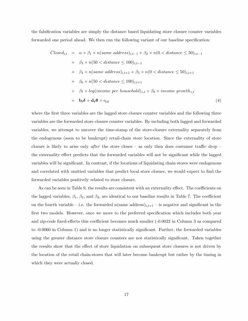
the falsification variables are simply the distance based liquidating store closure counter variables
forwarded one period ahead. We then run the following variant of our baseline specification:
Closedi,t = α+ β1 × n(same address)i,t−1 + β2 × n(0 < distance ≤ 50)i,t−1
+ β3 × n(50 < distance ≤ 100)i,t−1
+ β4 × n(same address)i,t+1 + β5 × n(0 < distance ≤ 50)i,t+1
+ β6 × n(50 < distance ≤ 100)i,t+1
+ β7 × log(income per household)z,t + β8 × income growthz,t
+ biδ + dtθ + εi,t (4)
where the first three variables are the lagged store closure counter variables and the following three
variables are the forwarded store closure counter variables. By including both lagged and forwarded
variables, we attempt to uncover the time-stamp of the store-closure externality separately from
the endogenous (soon to be bankrupt) retail-chain store location. Since the externality of store
closure is likely to arise only after the store closes – as only then does costumer traffic drop –
the externality effect predicts that the forwarded variables will not be significant while the lagged
variables will be significant. In contrast, if the locations of liquidating chain stores were endogenous
and correlated with omitted variables that predict local store closure, we would expect to find the
forwarded variables positively related to store closure.
As can be seen in Table 9, the results are consistent with an externality effect. The coefficients on
the lagged variables, β1, β2, and β3, are identical to our baseline results in Table 7. The coefficient
on the fourth variable – i.e. the forwarded n(same address)i,t+1 – is negative and significant in the
first two models. However, once we move to the preferred specification which includes both year
and zip-code fixed-effects this coefficient becomes much smaller (-0.0022 in Column 3 as compared
to -0.0060 in Column 1) and is no longer statistically significant. Further, the forwarded variables
using the greater distance store closure counters are not statistically significant. Taken together
the results show that the effect of store liquidation on subsequent store closures is not driven by
the location of the retail chain-stores that will later become bankrupt but rather by the timing in
which they were actually closed.
17

C. Stores Closings Inside Shopping Malls
Prior work has shown that anchor stores in shopping malls create positive externalities on other non-
anchor stores by attracting customer traffic. Mall owners internalize this externality by providing
rent subsidies to anchor stores. Indeed, the rent subsidy provided to anchor stores as compared to
non-anchor stores estimated at no less than 72 percent suggests that these positive externalities
are economically large. Given the importance of anchor stores within malls, we next focus our
analysis on the potential externalities that arise when an anchor store in a shopping mall closes.
To maintain our identification strategy, we focus only on the effects of anchor store closures that
are a result of the liquidation of a national retail chain.
We match our data on retail chain stores to Esri’s Major Shopping Centers, a panel dataset of
major U.S. shopping centers that lists the name and address of each of the malls and includes data
on gross leasable area in the mall, the number of stores, and the names of up to four anchor tenants
in the mall. There are 4,421 unique malls that are matched to 104,217 store-year observations. The
average mall has a gross leasable area (GLA) of 474,019 square feet (median=349,437) and ranges
from a 25th percentile of 259,086 sqf to a 75th percentile of 567,000 sqf. The matched malls span
all of the fifty states and the District of Columbia. Figure 8 presents the geographical distribution
of the malls that are matched to our data as well as the shopping mall gross leasable area.
Next, to estimate the externality generated by store closures within malls, we rerun our baseline
regressions only on stores that have been matched to the Esri Mall database. Similar to the baseline
regressions, our main dependent variable in this regression, same mall, is simply the number of
retail-chain stores in the mall that close due to the liquidation of the entire chain. Our data enable
us to control for mall fixed-effects (as opposed to just zip-code fixed effects) in addition to the year
dummies which further alleviates concerns about the initial location of stores of chains that end-up
in liquidation.
As Column 1 of Table 10 shows, we find that store closings within a mall lead to further store
closures within a mall. When a store closes in a mall, the subsequent annual closure rate of other
stores in the mall increases by 0.3 percentage points, or 4.9% of the sample mean. In Column 2
we add a second variable that counts the number of anchor stores within a mall that are closed as
a result of the liquidation of a national retail chain. As the table shows, we find that most of the
effect within malls is coming from anchor stores: The coefficient on same mall becomes insignificant
18

while that on the number of national liquidating anchor stores rises to 0.009. The effect of anchor
store closure is thus triple that of the average effect of non-anchor stores, consistent with prior
research pointing to the impact of anchor stores in drawing in costumers. The economic effect is
sizable with an anchor store closure causing a 14.7% increase in the probability of store closures
within the mall relative to the unconditional mean.
One caveat that should be noted in regards to this effect is that some firms insert co-tenancy
clauses into their lease contracts, which provide them the option to terminate their leases when
certain stores close. Thus, the increase in the externality effect could be explained both by the
greater importance of anchor stores in drawing traffic to malls, as well as the higher flexibility that
fellow stores enjoy in terminating their leases when an anchor store closes.
In a separate set of regressions, we also analyze the effect of store closures on stores located
outside malls. Table 11 repeats our baseline analysis in Table 7 for stores that were not matched
to the Esri’s Mall database. There are 550,364 stores in our data that are not part of matched
malls. Such stores are either not located in shopping malls, or are located in smaller malls that
are not matched to the Esri Mall database. As the table demonstrates, the coefficient on n(same
address)i,t−1 is positive and significant statistically indicating once again a negative externality of
store closure on stores located in the same address.12 Comparing the coefficients on the same-
address variable in Table 11 to those in Table 10 indicates that the effect of store closure outside
shopping malls on other stores located in the same address is similar to that of the effect of an
anchor store closure.13 One potential reason for this is that due to the small number of stores in
small shopping malls or in buildings where stores collocate, any store closure will have a relatively
large impact on other stores nearby.14
VI. Heterogeneity in the Response to Store Closures
In order to understand better the mechanisms through which store closures spread to further
closing of stores, we add heterogeneity to our empirical analysis. In this section we investigate the
12Note that retail stores collocating in the same address could either be stores not in a mall but in the samebuilding, or stores located in a mall which was not matched to the Esri database.
13Taking into account the standard errors of these coefficients shows that the coefficients are not statisticallydifferent for one another.
14This also explains why the coefficient on same address is larger when focusing on stores not matched to mallsthan the sample-wide effect of same address; The latter effect includes the impact of non-anchor store closure withinmalls, which as Table 10 shows, is small.
19

transmission of negative externalities that are imposed by bankruptcies of neighboring stores further
by studying the differential effect of store closures along the following three peer characteristics:
(i) across industries; (ii) conditional on a firm’s financial strength; and (iii) store size.
A. The Effect of Bankrupt Stores by Industry
We begin by analyzing whether the effect of store closures on neighboring store closures depends
on the industrial composition of stores in the same vicinity. Some spatial models of imperfect
competition predict that firms will choose to locate as far from their newest competitors as possible
(Chamberlin (1933), Nelson (1970), Salop (1979), Stuart (1979)). The key result of these models is
that the further away other stores are from a particular store, the greater market power that specific
store will have with respect to the consumers located near it. If so-called centrifugal competition
is the main factor driving stores locations in the U.S., we should expect that store closures will
benefit nearby stores that are in the same retail segment. This is simply because the remaining
stores will end up facing less competition.
Alternative spatial models suggest that it may be optimal for stores in the same industry to
locate next to one another. According to this view, the geographical concentration of similar stores
is driven by consumers’ imperfect information. For example, Wolinsky (1983) writes:
“[I]mperfectly informed consumers are attracted to a cluster of stores because that is
the best setting for search. A store may thus get more business and higher profits when
it is located next to similar stores. This effect may outweigh centrifugal competitive
forces...”15
Indeed, research in urban economics have provided a good deal of evidence for the existence of
economies of agglomeration and industrial clusters.16
To test how product substitutability and similarity influences the effect of retail store closures
on neighboring retail stores, we use the North American Industry Classification System (NAICS)
definition of an industry. To assign firms into industries, we employ two definitions that are based
on 5-digit and 6-digit NAICS codes.
Specifically, for each store in our sample we define same industry analogs of n(same address),
n(0<distance≤50), and n(50<distance≤100) which count only the number of liquidating retail-
15Wolinsky (1983) p. 274.16See for example, Ellison and Glaeser (1997), Henderson et al. (1995), and Rosenthal and Strange (2003)).
20

chain stores that are in the same industry of the given store, where industry identity is defined
using either 5- or 6-digit NAICS. For each store, we also define different industry exposures to
stores of liquidating national retail chains in an analogous manner. We then estimate, separately,
the effect of same industry and different industry store closures on subsequent store closings in their
area. Results that are based on 5-digit NAICS are presented in Table 12.
As the table shows, we find that the effect of same industry store closures is bigger than dif-
ferent industry store closures. In the specification that controls for year and zip-code fixed-effects
we find that the coefficient on n(same address) is 0.009 for same industry compared to 0.006 in
the different industry regression. Moreover, we also find a positive and significant effect of our
second distance measure, n(0<distance≤50), in the same industry regressions. This effect is quite
sizable: the coefficient of 0.018 (significant at the 5 percent level) in Column 3 implies that the
effect of having one store close increases the likelihood of further store closure by 29.5 percent
relative to the unconditional mean for stores in the same industry and that are located within a
50m radius of the closing store. In contrast, as Columns 4-6 show, there is no effect of different
industry n(0<distance≤50) on further store closures. We repeat the analysis using a 6-digit NAICS
definitions and obtain very similar results.17
B. Store Closures and Firm Profitability
We further investigate the transmission of negative externalities that are imposed by bankruptcies
of neighboring stores by studying the joint impact of a firms financial health and neighboring store
closures on the likelihood that a firm will close its own store. We hypothesize that the effect of
neighboring store closures on the likelihood that a store will close should be larger for stores owned
by parent firms that have low profitability. Less profitable firms are financially weaker, making
them more vulnerable to a decline in demand that is driven by the reduction in traffic associated
with neighboring stores closing down. We therefore introduce an interaction variable between
profitability and each of the local store closures into the specification estimated in the regressions
reported in Table 13.18
In Table 13 we run the analysis separately with different fixed-effects to control for geographic
heterogeneity. All regressions control for lagged values of firm size (natural log of book value of
17These results are omitted for brevity and are available upon request.18See Benmelech and Bergman (2011) for a similar approach.
21

assets), leverage (defined as total debt divided by lagged assets), and profitability (EBITDA divided
by assets).19 Column 1 of the table includes year fixed-effects, Column 2 includes year and state
fixed-effects, while Columns 3 and 4 each control for year and either county or zip-code fixed-effects.
As in the rest of the analysis in the paper, standard errors are clustered at the zip code level.
As can be seen in Table 13, the coefficients on all three measures of bankrupt stores – n(same
address), n(0<distance≤50), and n(50<distance≤100) – are positive and statistically significant,
indicating that stores closed in large retail-chain liquidations lead to additional store closures in their
vicinity. Consistent with the prediction of the joint effect of financial distress and store closures, we
find that the effect of local store closure is amplified when the retailer operating the neighboring
store is experiencing low profitability. The coefficients on the interaction terms between each of
the three distance measures and profitability is negative and significant suggesting that financially
stronger firms can weather the decline in revenue that is caused by store closings in the area.
More specifically, the estimates imply that a local store closure increases the likelihood that a
store in the same address with a parent firm in the 25th percentile of profitability will also close
by 1.03 to 1.36 percentage points, which represent an increase of 16.9 to 22.2 percent relative to
the unconditional mean. In contrast, when the parent of the store is in the 75th percentile of the
sample profitability, the effect of of store closure on the likelihood of same-address store closure is
not statistically different from zero. Similar to the effect of store closures on same-address stores,
the coefficient on the interaction term between n(0<distance≤50) and profitability is negative and
statistically significant at the ten percent level (the effect ranges from -0.0471 to -0.0485 ) with
standard errors of approximately 0.03) but only in the specification without county or zip code
fixed effects.20 Finally, the coefficient on the interaction term between n(50<distance≤100) and
profitability is negative and statistically significant in all specifications, including those with zip-
code fixed effects. The magnitude of the coefficients indicate that a store closure 50 to 100 meters
away increases the likelihood that a store with a parent in the 25th percentile of the profitability
distribution will close by 9.0 to 14.8 percent relative to the unconditional mean.
Moving to the firm-level variables, the results show that on average larger retailers are less
likely to close their stores while more leveraged retailers are more likely to close their stores.
Interestingly, we find that more profitable retailers are on average more likely to close their stores.
19Appendix A provides detailed definitions for each of the variables.20Note, though, that the coefficient on the interaction term barely changes across all specifications.
22

One explanation for this finding could be that more profitable firms are more likely to experiment
when choosing store locations, and hence are more likely to close stores which they find not to be
profitable.
Taken together, our results show that stores of weaker firms are strongly affected by the closure
of neighboring stores. The negative externality of store closure is greater on weaker firms than
on stronger ones and, as Table 13 shows, the effect carries over larger distances. Stores of weaker
firms thus seem to be more reliant on the existence of agglomeration economies. When these
agglomeration are destroyed through the liquidation of neighboring stores, weaker stores are pushed
towards economic inviability and shut down. Given an initial financial weakness in a geographic
area, store closures can thus propagates across the area.
C. Store Size and the Effect of Bankrupt Stores
We continue by analyzing how store size affects the impact of store closures on the decision of
neighboring stores to close. We hypothesize that a larger store will be more resilient to the closure
of neighboring stores as compared to a smaller store since larger stores may be less reliant on
neighboring stores to bring in costumer traffic. Further, to the extent that retailers act more quickly
to shut down unsuccessful large stores as compared to unsuccessful small stores, for example, due
to the greater impact larger stores have on retailers’ bottom line, larger stores will on average be
more profitable than smaller ones. Similar to the results in the prior section, we would then expect
larger stores to be more resilient to local store closures.
We rerun our baseline regressions analyzing the likelihood of store closure while interacting
store size, as measured by the number of employees in each store, with each of the three local store
closure variables, n(same address), n(0<distance≤50), and n(50<distance≤100). We add the usual
set of control variables which include the host of year and geographic fixed effects. The results are
reported in Table 14.
As can be seen in the table, we find a negative coefficient on the interaction term between store
size and the n(same address) variable which measures the number of store closures of liquidating
national retail chains in a given address. Consistent with our hypothesis, the negative coefficient
on the interaction term implies that larger stores are indeed less affected than smaller ones by
the closure of stores located in the same address. The economic effect is sizable: Focusing on the
specification with zip-code fixed effects, following the shutdown of a neighboring store, a store in
23

the 25th percentile of the size distribution experiences a 47 percent rise in the probability of closure
relative to the mean. In contrast, a store in the the 75th percentile of the size distribution expe-
riences only a 8.2 percent rise in the probability of closure. The data thus support the hypothesis
that larger stores are more resilient to neighboring store closures and less reliant on agglomeration
economies to generate traffic.
VII. Conclusion
Most empirical work on agglomeration economies focuses on the creation of economies of agglom-
eration through the endogenous choice of firm entry. In this paper, rather than focusing on the
endogenous creation of agglomeration economies we study how downturns damage economies of ag-
glomeration. Our analysis shows that bankrupt firms impose negative externalities on non-bankrupt
neighboring firms through the weakening of retail agglomeration economies. Store closures natu-
rally lead to reduced attractiveness of retail areas as customers prefer to shop in areas with full
occupancy. This, in turn, leads to declines in demand for retail services in the vicinity of bankrupt
stores, causing contagion from financially distressed companies to stores of non-bankrupt firms.
We argue that in downturns agglomeration economies may propagate bankruptcies and financial
distress.
24

Appendix A: Variable description and construction
This section documents the definitions of the variables used in the empirical analysis.
1. Market-to-book : total book value of assets (AT) plus the market value of equity (AT +
CSHO ∗ PRCCF ) minus the book value of equity deferred taxes (CEQ+TXDB), all over
total assets (AT*0.9) plus the market value of assets (MKVALT*0.1) (source: Compustat
Annual Fundamental files).
2. Leverage: total debt (DLTT+DLC+DCLO) divided by total assets (AT) (source: Compustat
Annual Fundamental files).
3. Profitability : EBITDA (OIBDP) divided by beginning-of-period total assets (AT) (source:
Compustat Annual Fundamental files).
4. Size: natural log of total assets (AT) (source: Compustat Annual Fundamental files).
25

References
Almazan, Andres, Adolfo De Motta, Sheridan Titman and Vahap Uysal, 2010. Financial Structure,
Acquisition Opportunities, and Firm Locations. The Journal of Finance, 65(2): 529-563.
Angrist, Joshua D and Jorn-Steffen Pischke, 2009, Mostly Harmless Econometrics, Princeton Uni-
versity Press, Princeton New Jersey.
Becker, Gary S. and Kevin M. Murphy. 1992. The Division of Labor, Coordination Costs, and
Knowledge. Quarterly Journal of Economics, 107(4): pp. 1137-1160.
Benmelech, E. and N. K. Bergman. 2011. Bankruptcy and the Collateral Channel. The Journal
of Finance, Vol. 66 No. 2: pp. 337-378.
Chamberlin, E. H., 1933, The Theory of Monopolistic Competition , Harvard University Press,
Cambridge, MA.
Cohen, Lauren, Andrea Frazzini and Christopher Malloy, 2008. The Small World of Investing:
Board Connections and Mutual Funds Returns. Journal of Political Economy, 116: 951-979.
Coval, Joshua and Tobias J. Moskowitz, 1999. Home Bias at Home: Local Equity Preference in
Domestic Portfolios. The Journal of Finance, 54(6): 2045-2073.
Ellison, Glenn and Edward Glaeser, 1997. Geographic Concentration in US Manufacturing Indus-
tries: A Dartboard Approach. Journal of Political Economy, 100: 1126-1152.
Ellison, Glenn and Edward Glaeser, 1999. The Geographic Concentration of US Industry: Does
Natural Advantage Explain Agglomeration? American Economic Review, 89(2): 1311-316.
Ellison, Glenn, Edward Glaeser and William Kerr, 2007. What Causes Industry Agglomeration?
Evidence from Coagglomeration Patterns. American Economic Review 100: 11951213.
Glaeser, Edward, Hedi D., Kallal, Jose A., Scheinkman and Andrei Shleifer, 1992. Growth in Cities.
Journal of Political Economy, 105(5): 889-927.
Gould, E.D. and B.P. Pashigian. 1998. Internalizing Externalities: The Pricing of Space in Shop-
ping Malls. Journal of Law and Economics, Vol. 41, No. 1: 115-142.
Gould, E.D., B.P. Pashigian and C. Prendergast. 2005. Contracts, Externalities, and Incentives in
Shopping Malls. The Review of Economics and Statistics, Vol. 87, No. 3: 411-422.
Greenstone, Michael, Richard Hornbeck, and Enrico Moretti, 2010. “Identifying Agglomeration
Spillovers: Evidence from Winners and Losers of Large Plant Openings”, Journal of Political
Economy, 118(3): 536-598.
Helsley, Roberts W., and William Strange. 1990. Matching and Agglomeration Economics in a
System of Cities. Regional Science and Urban Economics, 20(2): 189-212.
Henderson, Vernon, Ari Kuncoro, and Matt Turner, 1995. “Industrial Development in Cities”,
Journal of Political Economy, 103(5): 1067-1090.
Hotelling, H. 1929. Stability in Competition. Economic Journal, Vol. 39: 4157.
Krugman, P. 1991a, Geography and Trade, MIT Press, Cambridge, MA.
Krugman, P. 1991b. Increasing Returns and Economic Geography. Journal of Political Economy,
99(3): 483-499.
Leary, Mark and Michael Roberts, 2013. “Do Peer Firms Affect Corporate Financial Policy?”
Journal of Finance, forthcoming.
26

Lerner, Josh and Ulrike Malmendier. 2013. With a Little Help from My (Random) Friends: Success
and Failure in Post-Business School Entrepreneurship. Review of Financial Studies, 26(10): 2411-
2452.
Marshall, A. 1920. Principles of Economics; An Introductory Volume. Macmillan and Co.: London,
U.K.
Nelson, P., 1970. Information and Consumer Behavior. Journal of Political Economy, 78: 311-329.
Salop, S. C., 1979. Monopolistic Competition with Outside Goods. The Bell Journal of Economics,
Vol. 10, No. 1: 141-156.
Shue, Kelly. 2013. Executive Networks and Firm Policies: Evidence from the Random Assignment
of MBA Peers. Review of Financial Studies, 26(6): 1401-1442.
Wolinsky, A. 1983. Retail Trade Concentration Due to Consumers Imperfect Information. The
Bell Journal of Economics, Vol. 14, No. 1: 275-282.
Stuart C., 1979. “Search and Spatial Organization of Trading,” in S.A., Lipman and J.J., McCall.
ads. Studies in the Economics of Search, North-Holland, New York.
Stuart S. Rosenthal and William C. Strange, 2003. “Geography, Industrial Organization, and
Agglomeration,” The Review of Economics and Statistics, MIT Press, vol. 85(2), pages 377-393,
May.
Stuart S. Rosenthal and William C. Strange, 2008. “The Attenuation of Human Capital External-
ities,” Journal of Urban Economics, 64(2): 373-389.
27

Figure 1: Store locations as of 2005.
28

Figure 2: Store locations as of 2010.
29

Figure 3: Stores Closings during 2007.
30

Figure 4: Stores Closings during 2008.
31
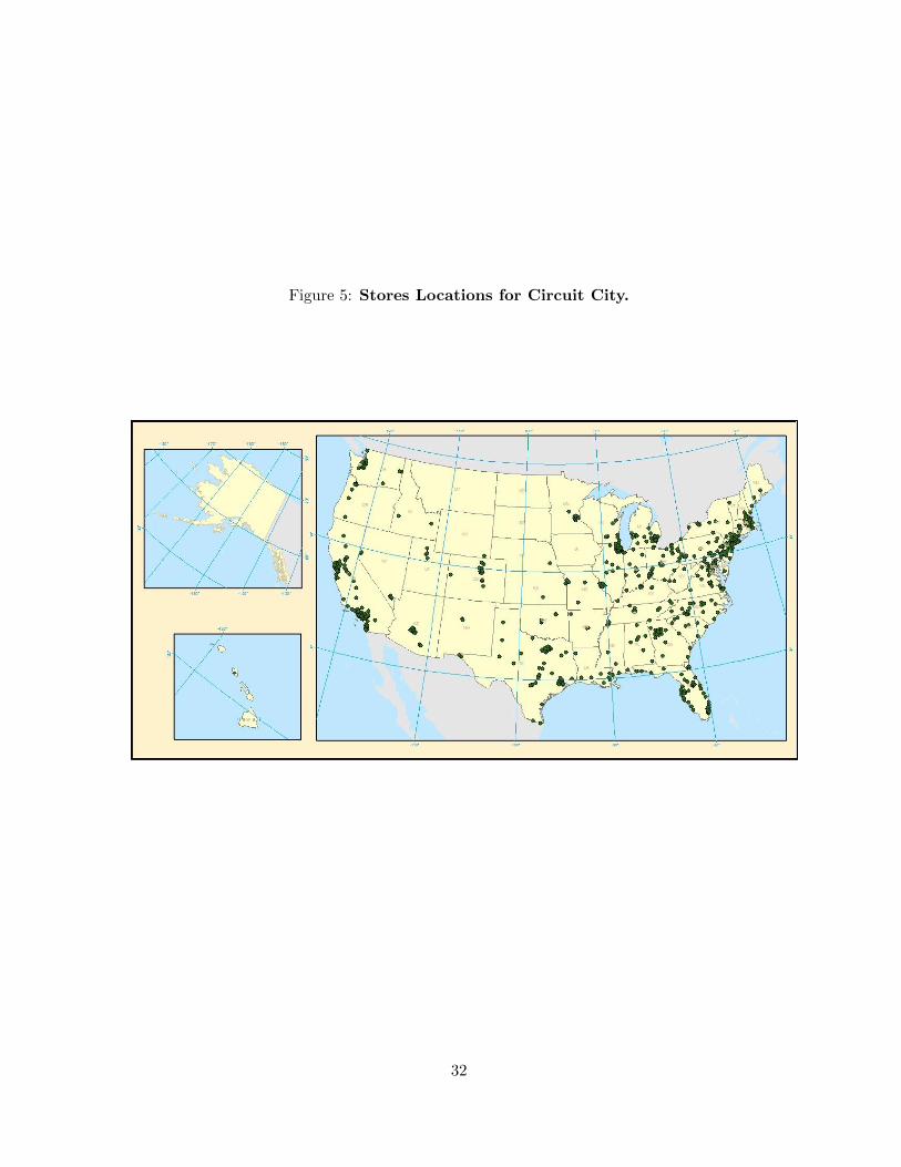
Figure 5: Stores Locations for Circuit City.
32

Figure 6: Stores Locations for Linens ‘N Things.
33

Figure 7: Stores Locations for The Sharper Image.
34

Figure 8: Shopping Malls location and size.
35

Table 1:Individual Store Closings
This table provides descriptive statistics on store closings and bankrupt stores. Panel A displays all store closings. Panel B presents
bankrupt stores, Panel C presents store closings that result from full liquidation bankruptcies. Variable definitions are provided in
Appendix A.
Panel A: Closed Stores over Time
25th 75th Standard
Year Mean Percentile Median Percentile Deviation Min Max Observations
2005-2009 0.061 0.0 0.0 0.0 0.239 0.0 1.0 661,382
2005 0.048 0.0 0.0 0.0 0.213 0.0 1.0 84,388
2006 0.085 0.0 0.0 0.0 0.279 0.0 1.0 125,897
2007 0.014 0.0 0.0 0.0 0.116 0.0 1.0 147,551
2008 0.110 0.0 0.0 0.0 0.313 0.0 1.0 148,432
2009 0.047 0.0 0.0 0.0 0.211 0.0 1.0 155,114
Panel B: Bankrupt Stores over Time
25th 75th Standard
Year Mean Percentile Median Percentile Deviation Min Max Observations
2005-2010 0.021 0.0 0.0 0.0 0.142 0.0 1.0 827,156
2005 0.010 0.0 0.0 0.0 0.100 0.0 1.0 84,388
2006 0.008 0.0 0.0 0.0 0.091 0.0 1.0 125,897
2007 0.029 0.0 0.0 0.0 0.167 0.0 1.0 147,551
2008 0.042 0.0 0.0 0.0 0.201 0.0 1.0 148,432
2009 0.026 0.0 0.0 0.0 0.158 0.0 1.0 155,114
2010 0.004 0.0 0.0 0.0 0.063 0.0 1.0 165,774
Panel C: Stores Closed in Full Liquidation Bankruptcies over Time
25th 75th Standard
Year Mean Percentile Median Percentile Deviation Min Max Observations
2005-2009 0.010 0.0 0.0 0.0 0.100 0.0 1.0 661,382
2005 0.002 0.0 0.0 0.0 0.049 0.0 1.0 84,388
2006 0.003 0.0 0.0 0.0 0.058 0.0 1.0 125,897
2007 0.001 0.0 0.0 0.0 0.033 0.0 1.0 147,551
2008 0.0186 0.0 0.0 0.0 0.135 0.0 1.0 148,432
2009 0.0193 0.0 0.0 0.0 0.137 0.0 1.0 155,114
36
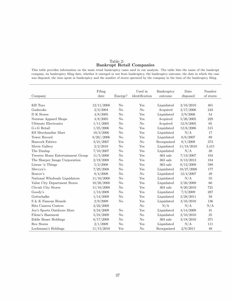
Table 2:Bankrupt Retail Companies
This table provides information on the main retail bankruptcy cases used in our analysis. The table lists the name of the bankrupt
company, its bankruptcy filing date, whether it emerged or not from bankruptcy, the bankruptcy outcome, the date in which the case
was disposed, the time spent in bankruptcy and the number of stores operated by the company in the time of the bankruptcy filing.
Filing Used in Bankruptcy Date Number
Company date Emerge? identification outcome disposed of stores
KB Toys 12/11/2008 No Yes Liquidated 2/16/2010 461
Gadzooks 2/3/2004 No No Acquired 2/17/2006 243
D K Stores 4/8/2005 No Yes Liquidated 2/9/2006 54
Norstan Apparel Shops 4/8/2005 No Yes Acquired 5/26/2005 229
Ultimate Electronics 1/11/2005 No No Acquired 12/9/2005 65
G+G Retail 1/25/2006 No Yes Liquidated 12/6/2006 515
KS Merchandise Mart 10/3/2006 No Yes Liquidated N/A 17
Tower Record 8/20//2006 No Yes Liquidated 8/6/2007 89
Hancock Fabrics 3/21/2007 Yes No Reorganized 8/1/2008 373
Movie Gallery 2/2/2010 No Yes Liquidated 11/18/2010 2,415
The Dunlap 7/10/2007 No Yes Liquidated N/A 38
Tweeter Home Entertainment Group 11/5/2008 No Yes 363 sale 7/13/2007 104
The Sharper Image Corporation 2/19/2008 No Yes 363 sale 8/13/2012 184
Linens ’n Things 5/2/2008 No Yes 363 sale 6/12/2009 589
Mervyn’s 7/29/2008 No Yes Liquidated 10/27/2008 177
Boscov’s 8/4/2008 No No Liquidated 12/4/2007 49
National Wholesale Liquidators 11/10/2008 No Yes Liquidated N/A 55
Value City Department Stores 10/26/2008 No Yes Liquidated 2/26/2009 66
Circuit City Stores 11/10/2008 No Yes 363 sale 9/20/2010 721
Goody’s 1/13/2009 No Yes Liquidated 7/3/2009 287
Gottschalks 1/14/2009 No Yes Liquidated 2/28/2011 58
S & K Famous Brands 2/9/2009 No Yes Liquidated 3/16/2010 136
Ritz Camera Centers 2/22/2009 No N/A N/A N/A
Joe’s Sports Outdoors More 3/24/2009 No Yes Liquidated 4/14/2009 31
Filene’s Basement 5/24/2009 No No Liquidated 2/10/2010 25
Eddie Bauer Holdings 6/17/2009 No No 363 sale 3/18/2010 371
Rex Stores 2/1/2009 No Yes Liquidated N/A 111
Loehmann’s Holdings 11/15/2010 Yes No Reorganized 2/9/2011 48
37

Table 3:Neighboring Store Closures
This table provides descriptive statistics on full liquidation closings of neighboring stores. Panel A displays store closings in the same
address. Panels B and C present store closings for 0-50 meter and 50-100 meter distances. Panel D lists summary statistics for distances
that are between 150 and 500 meter. Variable definitions are provided in Appendix A.
Panel A: Same address
25th 75th Standard
Year Mean Percentile Median Percentile Deviation Min Max Observations
2005-2010 0.028 0.0 0.0 0.0 0.181 0.0 3.0 827,156
2005 0.0 0.0 0.0 0.0 0.0 0.0 0.0 84,388
2006 0.002 0.0 0.0 0.0 0.045 0.0 1.0 125,897
2007 0.038 0.0 0.0 0.0 0.192 0.0 2.0 147,551
2008 0.016 0.0 0.0 0.0 0.127 0.0 2.0 148,432
2009 0.085 0.0 0.0 0.0 0.327 0.0 3.0 155,114
2010 0.009 0.0 0.0 0.0 0.100 0.0 2.0 165,774
Panel B: Not Same Address and Distance ≤ 50 meters
25th 75th Standard
Year Mean Percentile Median Percentile Deviation Min Max Observations
2005-2010 0.012 0.0 0.0 0.0 0.115 0.0 3.0 827,156
2005 0.0 0.0 0.0 0.0 0.0 0.0 0.0 84,388
2006 0.002 0.0 0.0 0.0 0.044 0.0 1.0 125,897
2007 0.009 0.0 0.0 0.0 0.099 0.0 2.0 147,551
2008 0.003 0.0 0.0 0.0 0.055 0.0 2.0 148,432
2009 0.038 0.0 0.0 0.0 0.207 0.0 3.0 155,114
2010 0.010 0.0 0.0 0.0 0.111 0.0 2.0 165,774
Panel C: 50 meters < distance ≤ 100 meters
25th 75th Standard
Year Mean Percentile Median Percentile Deviation Min Max Observations
2005-2010 0.008 0.0 0.0 0.0 0.094 0.0 3.0 827,156
2005 0.0 0.0 0.0 0.0 0.0 0.0 0.0 84,388
2006 0.001 0.0 0.0 0.0 0.030 0.0 1.0 125,897
2007 0.005 0.0 0.0 0.0 0.075 0.0 2.0 147,551
2008 0.002 0.0 0.0 0.0 0.044 0.0 1.0 148,432
2009 0.025 0.0 0.0 0.0 0.166 0.0 3.0 155,114
2010 0.008 0.0 0.0 0.0 0.103 0.0 2.0 165,774
Panel D: Further Away Store Closures 2005-2010
25th 75th Standard
Year Mean Percentile Median Percentile Deviation Min Max Observations
100 - 150 meters 0.007 0.0 0.0 0.0 0.087 0.0 3.0 827,156
150 - 200 meters 0.006 0.0 0.0 0.0 0.085 0.0 3.0 827,156
200 - 250 meters 0.020 0.0 0.0 0.0 0.151 0.0 4.0 827,156
250 - 300 meters 0.006 0.0 0.0 0.0 0.082 0.0 3.0 827,156
300 - 350 meters 0.006 0.0 0.0 0.0 0.083 0.0 4.0 827,156
350 - 400 meters 0.006 0.0 0.0 0.0 0.079 0.0 3.0 827,156
400 - 450 meters 0.006 0.0 0.0 0.0 0.081 0.0 3.0 827,156
450 - 500 meters 0.006 0.0 0.0 0.0 0.079 0.0 4.0 827,15638

Table 4:Retail Chains Fully Liquidated
This table provides information on the geographical dispersion of the liquidated retail chains used in the analysis.
Number Number Number Largest
Company of Stores of States of Census Divisions Census Division
Circuit City Stores 570 44 9 S. Atlantic
D K Stores 54 5 3 Mid Atlantic
Discovery Channel Retail Stores 107 32 9 Pacific
G+G Retail 314 40 9 S. Atlantic
Goody’s 377 21 5 S. Atlantic
Gottschalks 60 6 2 Pacific
Joe’s Sports Outdoors More 26 2 1 Pacific
KB Toys 483 44 9 Mid Atlantic
KS Merchandise Mart 18 5 3 E. N. Central
Linens ’n Things 496 48 9 S. Atlantic
Mervyn’s 169 8 3 Pacific
Movie Gallery 2,831 50 9 Pacific
National Wholesale Liquidators 44 12 4 Mid Atlantic
Norstan Apparel Shops 147 21 6 S. Atlantic
Rex Stores 113 34 9 S. Atlantic
S & K Famous Brands 43 11 5 S. Atlantic
The Dunlap 38 8 4 W. S. Central
The Sharper Image Corporation 178 38 9 Pacific
Tower Record 88 20 8 Pacific
Tweeter Home Entertainment Group 104 22 8 S. Atlantic
Value City Department Stores 105 15 5 E. N. Central
39

Table 5:Comparison of Store Locations
This table compares the means of log(Adjusted gross income), log(Median house value) and ∆(House value 2002-
2006) across all the stores of fully liquidated chains and similar chains that were not liquidated for a three selected
chains. Means are calculated based on store locations in 2006. p-values are calculated using a two-sample t-test
assuming equal variances for the hypothesis that the difference in the means is different from zero.
log(Adjusted gross log(Median ∆(House Number of stores
Company income) house value) value 2002-2006)
Circuit City Stores 4.08 11.81 0.63 607
Best Buy 4.09 11.82 0.60 729
p-value (0.799) (0.625) (0.164)
Linens ’n Things 4.12 11.91 0.61 511
Bed Bath & Beyond 4.11 11.87 0.60 700
p-value (0.308) (0.119) 0.598)
The Sharper Image 4.17 12.19 0.68 181
Brookstone 4.16 12.02 0.69 269
p-value (0.983) (0.00) (0.635)
40

Table 6:Determinants of Store Locations
This table presents coefficient estimates and standard errors in parentheses for linear probability models of stores locations. The
tables uses zip-code level economic controls and all regressions include an intercept, and county fixed effects (not reported). Standard
errors are calculated by clustering at the zip code level. ∗∗∗, ∗∗, and ∗ denote statistical significance at the 1%, 5%, and 10% levels,
respectively.
(1) (2) (3) (4) (5) (6)
All stores Non-Mall stores Mall stores All stores Non-Mall stores Mall stores
log(median household income) 0.0067 0.010 -0.017 -0.007 0.001 -0.035
(0.009) (0.010) (0.035) (0.007) (0.001) (0.030)
log(median house value) 0.002 0.004 -0.010 0.008*** 0.010*** -0.007
(0.003) (0.003) (0.011) (0.002) (0.002) (0.008)
Median house price growth, 0.0002 -0.0004 -0.003 -0.001 -0.001 -0.003
2002-2006 (0.004) (0.004) (0.016) (0.003) (0.003) (0.009)
Mall 0.037*** 0.028***
(0.003) (0.002)
Year 2005 2005 2005 2006 2006 2006
Fixed-effects County County County County County County
Observations 52,597 44,488 8,109 76,057 62,808 13,249
Adjusted-R-squared 0.013 0.010 0.043 0.002 0.007 0.030
41

Table 7:Neighboring Bankrupt Stores and Store Closures
This table presents coefficient estimates and standard errors in parentheses for linear probability models of store closures. All regressions
include an intercept and year fixed-effects. Models 2, 3, and 4 include state, county, and zip-code fixed-effects, respectively. Model 5
includes county*year and Model 6 includes zip*year fixed effects. Standard errors are calculated by clustering at the zip code level. ∗∗∗,
∗∗, and ∗ denote statistical significance at the 1%, 5%, and 10% levels, respectively.
(1) (2) (3) (4) (5) (6)
Full liquidation bankrupt stores closurest−1
same address 0.0036** 0.0037** 0.0042*** 0.0065*** 0.0030** 0.005***
(0.002) (0.002) (0.002) (0.002) (0.0015) (0.002)
distance ≤ 50 meters 0.0003 0.0005 0.0002 -0.0024 -0.001 -0.002
(0.002) (0.002) (0.002) (0.002) (0.002) (0.002)
50 meters < distance ≤ 100 meters 0.0019 0.0024 0.0022 0.0007 0.002 0.003
(0.003) (0.003) (0.003) (0.003) (0.003) (0.003)
Ln(income per household) 0.0066*** 0.0052*** -0.0049 -0.0650***
(0.002) (0.002) (0.003) (0.009)
Income growth -0.0328*** -0.0381*** -0.0304*** 0.0071
(0.009) (0.009) (0.009) (0.011)
Fixed-effects Year Year+State Year+County Year+Zip Year-by-County Year-by-Zip
Observations 654,581 654,581 654,581 654,581 654,581 654,581
Adjusted R-squared 0.021 0.021 0.027 0.062 0.050 0.160
42

Table 8:Neighboring Bankrupt Stores and Store Closures by Distance
This table presents coefficient estimates and standard errors in parentheses for linear probability models of store closures. All
regressions include an intercept and year fixed-effects. Models 2, 3, and 4 include state, county, and zip-code fixed-effects,
respectively. Standard errors are calculated by clustering at the zip code level. ∗∗∗, ∗∗, and ∗ denote statistical significance at
the 1%, 5%, and 10% levels, respectively.
(1) (2) (3) (4)
Full liquidation bankrupt stores closurest−1
same address 0.004** 0.004** 0.004*** 0.007***
(0.002) (0.002) (0.002) (0.002)
distance ≤ 50 meters 0.0002 0.0004 0.0002 -0.002
(0.002) (0.002) (0.002) (0.002)
50 meters < distance ≤ 100 meters 0.002 0.002 0.002 0.001
(0.003) (0.003) (0.003) (0.003)
100 meters < distance ≤ 150 meters 0.002 0.002 0.002 0.002
(0.004) (0.004) (0.004) (0.005)
150 meters < distance ≤ 200 meters 0.003 0.003 0.002 0.001
(0.005) (0.005) (0.005) (0.005)
200 meters < distance ≤ 250 meters -0.001 -0.000 -0.000 -0.003
(0.003) (0.003) (0.003) (0.003)
250 meters < distance ≤ 300 meters 0.003 0.004 0.003 0.001
(0.004) (0.004) (0.004) (0.004)
300 meters < distance ≤ 350 meters -0.003 -0.002 -0.003 -0.005*
(0.003) (0.003) (0.003) (0.003)
350 meters < distance ≤ 400 meters 0.002 0.003 0.003 0.000
(0.003) (0.003) (0.003) (0.003)
400 meters < distance ≤ 450 meters 0.004 0.005 0.004 0.001
(0.004) (0.004) (0.003) (0.003)
450 meters < distance ≤ 500 meters 0.005 0.005 0.002 -0.001
(0.007) (0.007) (0.006) (0.006)
Ln(income per household) 0.007*** 0.005*** -0.005 -0.065***
(0.002) (0.002) (0.003) (0.009)
Income growth -0.033*** -0.038*** -0.030*** 0.007
(0.009) (0.009) (0.009) (0.011)
Fixed-effects Year Year+State Year+County Year+Zip
Observations 654,581 654,581 654,581 654,581
Adjusted R-squared 0.021 0.022 0.027 0.062
43

Table 9:Neighboring Bankrupt Stores and Placebo Store Closures
This table presents coefficient estimates and standard errors in parentheses for linear probability placebo
models of store closures. All regressions include an intercept and year fixed-effects. Models 1, 2, and 3
include state, county, and zip-code fixed-effects, respectively. Standard errors are calculated by clustering at
the zip code level. ∗∗∗, ∗∗, and ∗ denote statistical significance at the 1%, 5%, and 10% levels, respectively.
(1) (2) (3)
Full liquidation bankrupt stores closurest−1
same address 0.004*** 0.005*** 0.007***
(0.002) (0.002) (0.002)
distance ≤ 50 meters 0.001 0.0002 -0.002
(0.002) (0.002) (0.002)
50 meters < distance ≤ 100 meters 0.002 0.002 0.001
(0.003) (0.003) (0.003)
Placebo full liquidation bankrupt stores closurest+1
same address -0.0060*** -0.0054*** -0.0022
(0.001) (0.001) (0.001)
distance ≤ 50 meters -0.0022 -0.0018 -0.0012
(0.002) (0.002) (0.002)
50 meters < distance ≤ 100 meters 0.0010 0.0015 0.0024
(0.003) (0.003) (0.003)
Ln(income per household) 0.0053*** -0.0046 -0.0647***
(0.002) (0.003) (0.009)
Income growth -0.0381*** -0.0305*** 0.0069
(0.009) (0.009) (0.011)
Fixed-effects Year+State Year+County Year+Zip
Observations 654,581 654,581 654,581
Adjusted R-squared 0.022 0.027 0.062
44

Table 10:Mall Bankrupt Stores and Mall Store Closures
This table presents coefficient estimates and standard errors in parentheses for linear probability models of
mall-based store closures. All regressions include an intercept and year and mall fixed-effects. Standard
errors are calculated by clustering at the zip code level. ∗∗∗, ∗∗, and ∗ denote statistical significance at the
1%, 5%, and 10% levels, respectively.
(1) (2)
Full liquidation bankrupt stores closurest−1
same mall 0.003* 0.002
(0.002) (0.002)
same mall anchor store 0.009**
(0.004)
Ln(income per household) -0.046* -0.048*
(0.027) (0.027)
Income growth 0.094** 0.095**
(0.038) (0.038)
Fixed-effects Year+Mall Year+Mall
Observations 104,217 104,217
Adjusted R2 0.094 0.094
45

Table 11:Non-Mall Bankrupt Stores and Non-Mall Store Closures
This table presents coefficient estimates and standard errors in parentheses for linear probability models of non-mall store
closures. All regressions include an intercept and year fixed-effects. Models 2, 3, and 4 include state, county, and zip-code
fixed-effects, respectively. Standard errors are calculated by clustering at the zip code level. ∗∗∗, ∗∗, and ∗ denote statistical
significance at the 1%, 5%, and 10% levels, respectively.
(1) (2) (3) (4)
Full liquidation bankrupt stores closurest−1
same address 0.0115*** 0.0118*** 0.0115*** 0.0087**
(0.004) (0.004) (0.004) (0.004)
distance ≤ 50 meters -0.0015 -0.0013 -0.0008 -0.0034
(0.003) (0.003) (0.003) (0.003)
50 meters < distance ≤ 100 meters 0.0053 0.0056 0.0060* 0.0039
(0.004) (0.004) (0.004) (0.003)
Ln(income per household) 0.0089*** 0.0071*** -0.0023 -0.0682***
(0.002) (0.002) (0.003) (0.009)
Income growth -0.0442*** -0.0491*** -0.0413*** 0.0002
(0.010) (0.011) (0.010) (0.011)
Fixed-effects Year Year+State Year+County Year+Zip
Observations 550,364 550,364 550,364 550,364
Adjusted R-squared 0.021 0.022 0.028 0.067
46

Table 12:Bankrupt Stores Industry and Store Closures (5-digit NAICS)
This table presents coefficient estimates and standard errors in parentheses for linear probability models of store closures. The tables
presents results for store closures in the same industry as well as store closures in different industries. All regressions include an intercept
and year fixed-effects. Models 1, 2, and 3 include state, county, and zip-code fixed-effects, respectively. Models 4, 5, and 6 also include
state, county, and zip-code fixed-effects, respectively. Standard errors are calculated by clustering at the zip code level. ∗∗∗, ∗∗, and ∗denote statistical significance at the 1%, 5%, and 10% levels, respectively.
(1) (2) (3) (4) (5) (6)
Full liquidation bankrupt stores closures same industryt−1
same address 0.008* 0.008* 0.009**
(0.004) (0.004) (0.004)
distance ≤ 50 meters 0.022** 0.022** 0.018**
(0.009) (0.009) (0.009)
50 meters < distance ≤ 100 meters 0.002 0.002 -0.004
(0.009) (0.009) (0.010)
Full liquidation bankrupt stores closures different industryt−1
same address 0.003** 0.004** 0.006***
(0.002) (0.002) (0.002)
distance ≤ 50 meters -0.001 -0.001 -0.004
(0.002) (0.002) (0.003)
50 meters < distance ≤ 100 meters 0.003 0.002 0.001
(0.003) (0.003) (0.003)
Ln(income per household) 0.005*** -0.005 -0.066*** 0.005*** -0.005 -0.065***
(0.002) (0.003) (0.009) (0.002) (0.003) (0.009)
Income growth -0.038*** -0.030*** 0.007 -0.038*** -0.030*** 0.007
(0.009) (0.009) (0.011) (0.009) (0.009) (0.011)
Fixed-effects Year+State Year+County Year+Zip Year+State Year+County Year+Zip
Observations 654,581 654,581 654,581 654,581 654,581 654,581
Adjusted R2 0.022 0.027 0.062 0.022 0.027 0.062
47

Table 13:Bankrupt Stores Firm Profitability and Store Closures
This table presents coefficient estimates and standard errors in parentheses for linear probability models of store closures conditional
on firm profitability. All regressions include an intercept and year fixed-effects. Models 2, 3, and 4 include state, county, and zip-code
fixed-effects, respectively. Standard errors are calculated by clustering at the zip code level. ∗∗∗, ∗∗, and ∗ denote statistical significance
at the 1%, 5%, and 10% levels, respectively.
(1) (2) (3) (4)
Full liquidation bankrupt stores closurest−1
same address 0.0329*** 0.0332*** 0.0345*** 0.0364***
(0.004) (0.004) (0.004) (0.004)
×Profitabilityt−1 -0.1679*** -0.1683*** -0.1709*** -0.1698***
(0.016) (0.016) (0.016) (0.016)
distance ≤ 50 meters 0.0110* 0.0116** 0.0109* 0.0066
(0.006) (0.006) (0.006) (0.006)
×Profitabilityt−1 -0.0478* -0.0485* -0.0471 -0.0475
(0.029) (0.029) (0.029) (0.030)
50 meters < distance ≤ 100 meters 0.0227*** 0.0233*** 0.0241*** 0.0205***
(0.008) (0.008) (0.008) (0.008)
×Profitabilityt−1 -0.1085*** -0.1082*** -0.1123*** -0.1114***
(0.037) (0.037) (0.037) (0.038)
Sizet−1 -0.0067*** -0.0068*** -0.0067*** -0.0066***
(0.000) (0.000) (0.000) (0.000)
Leveraget−1 0.1024*** 0.1027*** 0.1029*** 0.1043***
(0.003) (0.003) (0.003) (0.003)
Profitabilityt−1 0.0846*** 0.0853*** 0.0858*** 0.0859***
(0.006) (0.006) (0.006) (0.006)
Ln(income per household) 0.0076*** 0.0056** -0.0027 -0.0899***
(0.002) (0.002) (0.004) (0.011)
Income growth -0.0116 -0.0095 -0.0089 0.0415***
(0.013) (0.013) (0.013) (0.016)
Fixed-effects Year Year+State Year+County Year+Zip
Observations 359,675 359,675 359,675 359,675
Adjusted R2 0.030 0.030 0.040 0.090
48

Table 14:Store Size and Store Closures
This table presents coefficient estimates and standard errors in parentheses for linear probability models of store closures conditional on
store size. All regressions include an intercept and year fixed-effects. Models 2, 3, and 4 include state, county, and zip-code fixed-effects,
respectively. Standard errors are calculated by clustering at the zip code level. ∗∗∗, ∗∗, and ∗ denote statistical significance at the 1%,
5%, and 10% levels, respectively.
(1) (2) (3) (4)
Full liquidation bankrupt stores closurest−1
same address 0.058*** 0.059*** 0.060*** 0.050***
(0.009) (0.009) (0.009) (0.010)
×Store size -0.014*** -0.014*** -0.014*** -0.012***
(0.002) (0.002) (0.002) (0.002)
distance ≤ 50 meters -0.007 -0.007 -0.006 -0.010
(0.010) (0.011) (0.011) (0.011)
×Store size 0.003 0.003 0.003 0.003
(0.003) (0.003) (0.003) (0.003)
50 meters < distance ≤ 100 meters -0.001 -0.001 0.001 -0.001
(0.009) (0.009) (0.009) (0.009)
×Store size -0.0002 -0.0001 -0.001 -0.001
(0.002) (0.002) (0.002) (0.002)
Store size -0.004*** -0.004*** -0.004*** -0.005***
(0.000) (0.000) (0.000) (0.000)
Ln(income per household) 0.0001 -0.001 -0.007* -0.023
(0.002) (0.002) (0.004) (0.014)
Income growth 0.032** 0.029* 0.027* 0.037**
(0.015) (0.015) (0.015) (0.015)
Fixed-effects Year Year+State Year+County Year+Zip
Observations 181,066 181,066 181,066 181,066
Adjusted R2 0.016 0.017 0.030 0.121
49
![Iron Ore Agglomeration Technologies · form briquettes [8]. A traditional application is the agglomeration of coal [8], other example is the agglomeration of ultrafine oxidized dust](https://img.pdfslide.us/doc/110x75/5e858e2963f1fe02e5184012/iron-ore-agglomeration-technologies-form-briquettes-8-a-traditional-application.jpg)