Recent experiments on the aerodynamics and forcesexperienced by model flapping insect wings have allowed greatleaps in our understanding of the mechanisms of insect flight.‘Delayed stall’ creates a leading-edge vortex that accounts fortwo-thirds of the required lift during the downstroke of ahovering hawkmoth (Ellington et al., 1996; Van den Berg andEllington, 1997b). Maxworthy (1979) identified such a vortexduring the ‘quasi-steady second phase of the fling’ in a flappingmodel, but its presence and its implications for lift productionby insects using a horizontal stroke plane have only been realisedafter the observations of smoke flow around tethered (Willmottet al., 1997) and mechanical (Van den Berg and Ellington,1997a,b) hawkmoths. Additional mechanisms, ‘rotationalcirculation’ (referring to rotation about the pronation/supinationaxis) and ‘wake capture’, described for a model Drosophila,account for further details of force production, particularlyimportant in control and manoeuvrability (Dickinson et al.,1999; Sane and Dickinson, 2001).

Experiments based on flapping models are the best way atpresent to investigate the unsteady and three-dimensionalaspects of flapping flight. The effects of wing–wing interaction,wing rotation about the supination/pronation axis, wingacceleration and interactions between the wing and the induced

flow field can all be studied with such models. However,experiments with flapping models inevitably confound someor all of these variables. To investigate the properties of theleading-edge vortex over ‘revolving’ wings, while avoidingconfounding effects from wing rotation (pronation andsupination) and wing–wing interaction, this study is based ona propeller model. ‘Revolving’ in this study refers to therotation of the wings about the body, as in a propeller. Theconventional use of the term ‘rotation’ in studies of insectflight, which refers to pronation and supination, is maintained.A revolving propeller mimics, in effect, the phase of a down-(or up-) stroke between periods of wing rotation.

The unusually complete kinematic and morphological dataavailable for the hovering hawkmoth Manduca sexta(Willmottand Ellington, 1997b), together with its relatively large size,have made this an appropriate model insect for previousaerodynamic studies. This, and the potential for comparisonswith computational (Liu et al., 1998) and mechanical flappingmodels, both published and current, make Willmott andEllington’s (1997b) hovering hawkmoth an appropriatestarting point for propeller experiments.

This study assesses the influences of leading-edge detail,twist and camber on the aerodynamics of revolving wings. The

1547The Journal of Experimental Biology 205, 1547–1564 (2002)Printed in Great Britain © The Company of Biologists Limited 2002JEB4262

Recent work on flapping hawkmoth models hasdemonstrated the importance of a spiral ‘leading-edgevortex’ created by dynamic stall, and maintained by someaspect of spanwise flow, for creating the lift requiredduring flight. This study uses propeller models toinvestigate further the forces acting on model hawkmothwings in ‘propeller-like’ rotation (‘revolution’). Steadilyrevolving model hawkmoth wings produce high vertical(≈ lift) and horizontal (≈ profile drag) force coefficientsbecause of the presence of a leading-edge vortex. Bothhorizontal and vertical forces, at relevant angles of attack,are dominated by the pressure difference between theupper and lower surfaces; separation at the leading edgeprevents ‘leading-edge suction’. This allows a simple

geometric relationship between vertical and horizontalforces and the geometric angle of attack to be derived forthin, flat wings. Force coefficients are remarkablyunaffected by considerable variations in leading-edgedetail, twist and camber. Traditional accounts of theadaptive functions of twist and camber are based onconventional attached-flow aerodynamics and are notsupported. Attempts to derive conventional profile dragand lift coefficients from ‘steady’ propeller coefficients arerelatively successful for angles of incidence up to 50 ° and,hence, for the angles normally applicable to insect flight.

Key words: aerodynamics, Manduca sexta, propeller, hawkmoth,model, leading-edge vortex, flight, insect, lift, drag.

Summary

Introduction

The aerodynamics of revolving wings

I. Model hawkmoth wings

James R. Usherwood* and Charles P. EllingtonDepartment of Zoology, University of Cambridge, Downing Street, Cambridge CB2 3EJ, UK

*Present address: Concord Field Station, MCZ, Harvard University, Old Causeway Road, Bedford, MA 01730, USA(e-mail: jimusherwood@lycos.co.uk)

Accepted 21 March 2002

1548

similarities between the leading-edge vortex over flappingwings and those found over swept and delta wings operatingat high angles of incidence (Van den Berg and Ellington,1997b) suggest that the detail of the leading edge may be ofinterest (Lowson and Riley, 1995): the sharpness of the leadingedge of delta wings is critical in determining the relationshipbetween force coefficients and angle of attack. Protuberancesfrom the leading edge are used on swept-wing aircraft to delayor control the formation of leading-edge vortices (see Ashill etal., 1995; Barnard and Philpott, 1995). Similar protuberancesat a variety of scales exist on biological wings, from the finesawtooth leading-edge of dragonfly wings (Hertel, 1966) to theadapted digits of birds (the alula), bats (thumbs) and some, butnot all, sea-turtles and pterosaurs. The effect of a highlydisrupted leading edge is tested using a ‘sawtooth’ variation onthe basic hawkmoth planform.

Willmott and Ellington (1997b) observed wing twistsof 24.5 ° (downstroke) to 19 ° (upstroke) in the hoveringhawkmoth F1, creating higher angles of attack at the base thanat the tip for both up- and downstroke. Such twists are typicalfor a variety of flapping insects (e.g. Jensen, 1956; Norberg,1972; Weis-Fogh, 1973; Wootton, 1981; Ellington, 1984c), but

this is not always the case (Vogel, 1967a; Nachtigall, 1979).The hawkmoth wings were also seen to be mildly cambered,agreeing with observations for a variety of insects; see, forinstance, photographs by Dalton (1977) or Brackenbury(1995). Both these features of insect wings have been assumedto provide aerodynamic benefits (e.g. Ellington, 1984c) andhave been shown to be created by largely passive, but intricate,mechanical deflections (Wootton, 1981, 1991, 1992, 1993,1995; Ennos, 1988).

Previous studies of the effects of camber have had mixedresults. Camber on conventional aircraft wings increases themaximum lift coefficients and normally improves the lift-to-drag ratio. This is also found to be true for locust (Jensen,1956), Drosophila(Vogel, 1967b) and bumblebee (Dudley andEllington, 1990b) wings. However, the effects of camber onunsteady wing performance appear to be negligible (Dickinsonand Götz, 1993).

The propeller rig described here enables the aerodynamicconsequences of leading-edge vortices to be studied. It alsoallows the importance of various wing features, previouslydescribed by analogy with conventional aerofoil or propellertheory, to be investigated.

J. R. Usherwood and C. P. Ellington

ii

iii

iv

v

vi

vii i

100 mm

i

vii

ix

A

Vertical forcestrain gauges

CounterweightStop Propeller body

Knife-bladefulcrum

1 m

Stiffeningwire

B

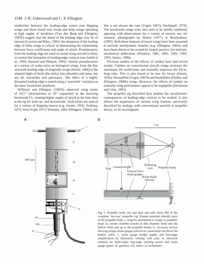
Fig. 1. Propeller body (A) and plan and side views (B) of thecomplete ‘see-saw’ propeller rig. Roman numerals identify partsof the propeller body. i, sting for attachment to wings; ii, propellerhead; iii, smoke chamber (smoke in this chamber feeds into thehollow shaft and up to the propeller head); iv, cut-away sectionshowing torque strain gauges (electrical connections run down thehollow axle); v, strain gauge bridge supply and first-stageamplification by electronics rotating with axle; vi, electricalcontacts on multi-wiper slip-rings carrying power and straingauge signal; vii, gearbox; viii, motor; ix, tachometer.

1549Aerodynamics of hawkmoth wings in revolution

Materials and methodsThe experimental propeller

A two-winged propeller (Fig. 1) was designed and built toenable both the quantitative measurement of forces and thequalitative observation of the flows experienced by propellerblades (or ‘wings’) as they revolve.

The shaft of the propeller was attached via a 64:1 spurgearbox to a 12 V Escap direct-current motor/tachometerdriven by a servo with tachometer feedback. The input voltagewas ramped up over 0.8 s; this was a compromise betweenapplying excessive initial forces (which may damage thetorque strain gauges and which set off unwanted mechanicalvibrations) and achieving a steady angular velocity as quicklyas possible (over an angle of 28 °). The voltage across thetachometer was sampled together with the force signals (seebelow) at 50 Hz. Angular velocity during the experiments wasdetermined from the tachometer signal, so any small deviationsin motor speed (e.g. due to higher torques at higher angles ofattack) were accounted for.

The mean Reynolds number (Re) for a flapping wing is asomewhat arbitrary definition (e.g. Ellington, 1984f; Van denBerg and Ellington, 1997a), but it appears unlikely that thehovering hawkmoths of Willmott and Ellington (1997a–c)were operating anywhere near a critical value: both larger andsmaller insects can hover in a fundamentally similar way;wing stroke amplitude, angle of attack and stroke plane areconsistent for the wide range of insects that undertake ‘normalhovering’ (Weis-Fogh, 1973; Ellington, 1984c). Because of

this, and the benefits in accuracy when using larger forces, afairly high rotational frequency (0.192 Hz) was chosen.Following the conventions of Ellington (1984f), this producesan Reof 8071. While this is a little higher than that derivedfrom the data of Willmott and Ellington (1997b) for F1(Re=7300), the hawkmoth selected below for a ‘standard’wing design, it is certainly within the range of hoveringhawkmoths.

Wing design

The wings were constructed from 500 mm×500 mm×2.75 mm sheets of black plastic ‘Fly-weight’ envelopestiffener. This material consists of two parallel, square, flatsheets sandwiching thin perpendicular lamellae that runbetween the sheets for the entire length of the square. Theorientation of these lamellae results in hollow tubes of squarecross section running between the upper and lower sheets fromleading to trailing edge. Together, this structure and materialproduces relatively stiff, light, thin, strong wing models.

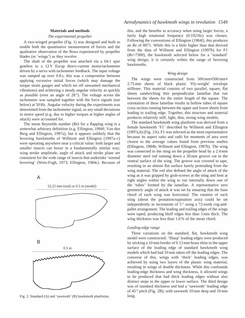
The standard hawkmoth wing planform was derived from afemale hawkmoth ‘F1’ described by Willmott and Ellington(1997a,b) (Fig. 2A). F1 was selected as the most representativebecause its aspect ratio and radii for moments of area wereclosest to the average values found from previous studies(Ellington, 1984b; Willmott and Ellington, 1997b). The wingwas connected to the sting on the propeller head by a 2.4 mmdiameter steel rod running down a 20 mm groove cut in theventral surface of the wing. The groove was covered in tape,resulting in an almost flat surface barely protruding from thewing material. The rod also defined the angle of attack of thewing as it was gripped by grub-screws at the sting and bent atright angles within the wing to run internally down one ofthe ‘tubes’ formed by the lamellae. A representative zerogeometric angle of attack α was set by ensuring that the basechord of each wing was horizontal. The rotation of eachsting (about the pronation/supination axis) could be setindependently in increments of 5 ° using a 72-tooth cog-and-pallet arrangement. The leading and trailing edges of the wingswere taped, producing bluff edges less than 3 mm thick. Thewing thickness was less than 1.6 % of the mean chord.

Leading-edge range

Three variations on the standard, flat, hawkmoth wingmodel were constructed. ‘Sharp’ leading edges were producedby sticking a 10 mm border of 0.13 mm brass shim to the uppersurface of the leading edge of standard hawkmoth wingmodels which had had 10 mm taken off the leading edges. Theconverse of this, wings with ‘thick’ leading edges, wasachieved by using two layers of the plastic wing material,resulting in wings of double thickness. While this confoundsleading-edge thickness and wing thickness, it allowed wingsto be produced that had thick leading edges without alsodistinct steps in the upper or lower surface. The third designwas of standard thickness and had a ‘sawtooth’ leading edgeof 45 ° pitch (Fig. 2B), with sawteeth 10 mm deep and 10 mmlong.Fig. 2. Standard (A) and ‘sawtooth’ (B) hawkmoth planforms.

A

B

52.25 mm (real) or 0.5 m (model)

0.5 m

1550

Twist range

Twisted wing designs were produced by introducing asecond 2.4 mm diameter steel rod, which ran down the centralgroove, with bends at each end running perpendicularly downinternal tubes at the wing base and near the tip. The two endsof the rod were out of plane, thus twisting the wing, creatinga lower angle of attack at the wing tip than at the base. Onewing pair had a twist of 15 ° between base and tip, while thesecond pair had a twist of 32 °. No measurable camber wasgiven to the twisted wings.

The wing material was weakened about the longitudinal axisof the wing by alternately slicing dorsal and ventral surfaces,which destroyed the torsion box construction of the internal‘tubes’. This slicing was necessary to accommodate theconsiderable shear experienced at the trailing and leadingedges, far from the twist axis.

Camber range

Standard hawkmoth wing models were heat-moulded toapply a camber. The wings were strapped to evenly curvedsteel sheet templates and placed in an oven at 100 °C forapproximately 1 h. The wings were then allowed to coolovernight. The wings ‘uncambered’ to a certain extent onremoval from the templates, but the radius of curvatureremained fairly constant along the span, and the reportedcambers for the wings were measured in situ on the propeller.For thin wings, camber can be described as the ratio of wingdepth to chord. One wing pair had a 7 % camber over the basalhalf of the wing: cambers were smaller at the tip because ofthe narrower chord. The second wing pair had a 10 % camberover the same region. The application of camber also gave asmall twist of less that 6 ° to the four wing models.

Wing moments

The standard wing shape used was a direct copy of thehawkmoth F1 planform except in the case of the sawtoothleading-edge design. However, the model wings do not revolveexactly about their bases: the attachment ‘sting’ and propellerhead displace each base by 53.5 mm from the propeller axis.Since the aerodynamic forces are influenced by both the wingarea and its distribution along the span, this offset must betaken into account.

Table 1 shows the relevant wing parameters foraerodynamic analyses, following Ellington’s (1984b)conventions. The total wing area S (for two wings) can berelated to the single wing length R and the aspect ratio AR:

S= 4R2/AR. (1)

Aerodynamic forces and torques are proportional to the secondand third moments of wing area, S2 and S3 respectively (Weis-Fogh, 1973). Non-dimensional radii, r2(S) and r3(S),corresponding to these moments are given by:

r2(S) = (S2/SR2)1/2 (2)and

r3(S) = (S3/SR3)1/3. (3)

Non-dimensional values are useful as they allow differences inwing shape to be identified while controlling for wing size.

The accuracy of the wing-making and derivation ofmoments was checked after the experiments by photographingand analysing the standard ‘flat’ hawkmoth wing. Differencesbetween the expected values of S2 and S3 for the model wingsand those observed after production were less than 1 %.

Smoke observations

Smoke visualisation was performed independently fromforce measurements. Vaporised Ondina EL oil (Shell, UK)from a laboratory-built smoke generator was fed into achamber of the propeller body and from there into the hollowshaft. This provided a supply of smoke at the propeller head,even during continuous revolution. Smoke was then deliveredfrom the propeller head to the groove in the ventral surface ofthe wing by 4.25 mm diameter Portex tubing. A slight pressurefrom the smoke generator forced smoke to disperse down thegroove, down the internal wing ‘tubes’ and out of the leadingand trailing edges of the wing wherever the tape had beenremoved. Observations were made directly or via a videocamera mounted directly above the propeller. Photographswere taken using a Nikon DS-560 digital camera with 50 mmlens. Lighting was provided by 1 kW Arri and 2.5 kW Castorspotlights. A range of rotational speeds was used: the basicflow properties were the same for all speeds, but a compromisespeed was necessary. At high speeds, the smoke spread toothinly to photograph, while at low speeds the smoke jetted clearof the boundary layer and so failed to label any vortices nearthe wing. A wing rotation frequency of 0.1 Hz was used for thephotographs presented here.

Force measurements

Measurement of vertical force

The propeller body was clamped to a steel beam by a brasssleeve. The beam projected horizontally, perpendicular to thepropeller axis, over a steel base-plate (Fig. 1B). The beam(1.4 m long, 105 mm deep and 5 mm wide) rested on a knife-blade fulcrum, which sat in a grooved steel block mounted onthe base-plate. Fine adjustment of the balance using acounterweight allowed the beam to rest gently on a steel shimcantilever with foil strain gauges mounted on the upper andlower surfaces. The shim was taped firmly to the beam and

J. R. Usherwood and C. P. Ellington

Table 1.Wing parameters for real and model hawkmoth wings

Model Model sawtooth hawkmoth wing hawkmoth wing

Hawkmoth F1 with offset with offset

R (mm) 52.25 556 556AR 5.66 6.34 6.33r2(S) 0.511 0.547 0.547r3(S) 0.560 0.588 0.588

R, wing length; AR, aspect ratio; r2(S), r3(S), non-dimensional second and third moments of area.

1551Aerodynamics of hawkmoth wings in revolution

deflected in response to vertical forces acting on the propelleron the other side of the fulcrum because of the ‘see-saw’configuration. The strain gauges were protected from excessivedeflection by a mechanical stop at the end of the beam. Signalsfrom these ‘vertical force’ strain gauges were amplified and fedinto a Macintosh Quadra 650 using LabVIEW to sample at50 Hz. The signal was calibrated using a 5 g mass placed at thebase of the propeller, directly in line with the propeller axis.No hysteresis between application and removal of the masswas observed, and five calibration measurements were madebefore and after each experiment. The mean coefficient ofvariation for each group of five measurements was less than2 %, and there was never a significant change betweencalibrations before and after each experiment.

The upper edge of the steel beam was sharpened underneaththe area swept by the propeller wings to minimise aerodynamicinterference. The beam was also stiffened by a diamondstructure of cables, separated by a 10 mm diameter aluminiumtube sited directly over the fulcrum.

Measurement of torque

The torque Q required to drive the wings was measured viaa pair of strain gauges mounted on a shim connected to the axleof the propeller (Fig. 1, iv). The signal from these strain gaugeswas pre-amplified with revolving electronics, also attached tothe shaft, before passing through electrical slip-rings (throughwhich the power supply also passed) machined from circuitboard. The signal was then amplified again before being passedto the computer, as with the vertical force signal.

The torque signal was calibrated by applying a knowntorque: a 5 g mass hung freely from a fine cotton thread, whichpassed over a pulley and wrapped around the propeller head.This produced a 49.1 mN force at a distance of 44 mm fromthe centre of the axle and resulted in a calibration torque of2.16 mN m. This procedure was extremely repeatable andshowed no significant differences throughout the experiments.Five calibration readings were recorded before and after eachexperiment. The mean coefficient of variation for each groupof five measurements was less than 6 %.

Torques due to friction in the bearings above the straingauges and to aerodynamic drag other than that caused by thewings were measured by running the propeller without wings.This torque was subtracted from the measurements with wings,giving the torque due to the wing drag only. It is likely,however, that this assessment of non-aerodynamic torque isnear the limit of the force transducers, and is somewhatinaccurate, because the aerodynamic drag measured for wingsat zero angle of incidence was apparently slightly less thanzero.

Experimental protocol

Each wing type was tested twice for a full range of anglesof attack from –20 to +95 ° with 5 ° increments and three timesusing an abbreviated test, covering from –20 ° to +100 ° in 20 °increments. Four runs were recorded at each angle of attack,consisting of approximately 10 s before the motor was turned

–1.2

–0.5

32

3.8

0

0.5

1.0

1.5

2.0

2.5

3.0

3.5

0

4

8 12 16 20 24 28

Sig

nal (

V)

Time (s)

ii i

C2

–12

–10

–8

–6

–4

–2

0

600 10 20 30 40 50

Sig

nal (

V)

Time (s)

2

–12

–10

–8

–6

–4

–2

0

0 10 20 30 40 50

Sig

nal (

V)

60

A

B

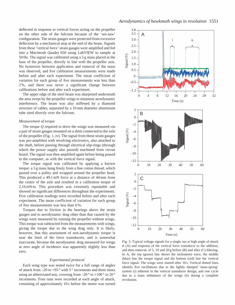
Fig. 3. Typical voltage signals for a single run at high angle of attackα (A) and response of the vertical force transducer to the addition,and then removal, of 5, 10 and 20 g before (B) and after (C) filtering.In A, the top (green) line shows the tachometer trace, the middle(blue) line the torque signal and the bottom (red) line the verticalforce signal. The wings were started after 10 s. Vertical dotted linesidentify five oscillations due to the lightly damped ‘mass-spring’system (i) inherent in the vertical transducer design, and one cycledue to a mass imbalance of the wings (ii) during a completerevolution.

1552

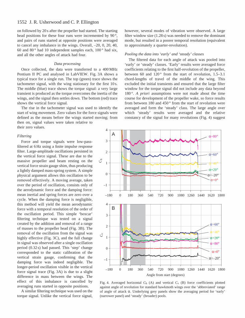
on followed by 20 s after the propeller had started. The startinghead positions for these four runs were incremented by 90 °,and pairs of runs started at opposite positions were averagedto cancel any imbalance in the wings. Overall, –20, 0, 20, 40,60 and 80 ° had 10 independent samples each, 100 ° had six,and all the other angles of attack had four.

Data processing

Once collected, the data were transferred to a 400 MHzPentium II PC and analysed in LabVIEW. Fig. 3A shows atypical trace for a single run. The top (green) trace shows thetachometer signal, with the wing stationary for the first 10 s.The middle (blue) trace shows the torque signal: a very largetransient is produced as the torque overcomes the inertia of thewings, and the signal then settles down. The bottom (red) traceshows the vertical force signal.

The rise in the tachometer signal was used to identify thestart of wing movement. Zero values for the force signals weredefined as the means before the wings started moving; fromthen on, signal values were taken relative totheir zero values.

Filtering

Force and torque signals were low-pass-filtered at 6 Hz using a finite impulse responsefilter. Large-amplitude oscillations persisted inthe vertical force signal. These are due to themassive propeller and beam resting on thevertical force strain gauge shim, thus producinga lightly damped mass-spring system. A simplephysical argument allows this oscillation to beremoved effectively. A moving average, takenover the period of oscillation, consists only ofthe aerodynamic force and the damping force:mean inertial and spring forces are zero over acycle. When the damping force is negligible,this method will yield the mean aerodynamicforce with a temporal resolution of the order ofthe oscillation period. This simple ‘boxcar’filtering technique was tested on a signalcreated by the addition and removal of a rangeof masses to the propeller head (Fig. 3B). Theremoval of the oscillation from the signal washighly effective (Fig. 3C), and the full changein signal was observed after a single oscillationperiod (0.32 s) had passed. This ‘step’ changecorresponded to the static calibration of thevertical strain gauge, confirming that thedamping force was indeed negligible. Thelonger-period oscillation visible in the verticalforce signal trace (Fig. 3A) is due to a slightdifference in mass between the wings. Theeffect of this imbalance is cancelled byaveraging runs started in opposite positions.

A similar filtering technique was used on thetorque signal. Unlike the vertical force signal,

however, several modes of vibration were observed. A largefilter window size (1.28 s) was needed to remove the dominantmode, but resulted in a poorer temporal resolution (equivalentto approximately a quarter-revolution).

Pooling the data into ‘early’ and ‘steady’ classes

The filtered data for each angle of attack was pooled into‘early’ or ‘steady’ classes. ‘Early’ results were averaged forcecoefficients relating to the first half-revolution of the propeller,between 60 and 120 ° from the start of revolution, 1.5–3.1chord-lengths of travel of the middle of the wing. Thisexcluded the initial transients and ensured that the large filterwindow for the torque signal did not include any data beyond180 °. A priori assumptions were not made about the timecourse for development of the propeller wake, so force resultsfrom between 180 and 450 ° from the start of revolution wereaveraged and form the ‘steady’ class. The large angle overwhich ‘steady’ results were averaged and the relativeconstancy of the signal for many revolutions (Fig. 4) suggest

J. R. Usherwood and C. P. Ellington

A

–180 0 180 360 540 720 900 1080 1260 1440 1620 1800

Ch

–1

0

1

2

3

4

α=40°

α=80°

α=60°

α=0°

α=20°α=–20°

B

Angle from start (degrees)

–180 0 180 360 540 720 900 1080 1260 1440 1620 1800

Cv

–1

0

1

2

3

4

α=–20°

α=0°

α=20°

α=40°

α=60°

α=80°

Fig. 4. Averaged horizontal Ch (A) and vertical Cv (B) force coefficients plottedagainst angle of revolution for standard hawkmoth wings over the ‘abbreviated’ rangeof angle of attack α. Underlying grey panels show the averaging period for ‘early’(narrower panel) and ‘steady’ (broader) pools.

1553Aerodynamics of hawkmoth wings in revolution

that the ‘steady’ results are close to those that would be foundfor propellers that have achieved steady-state revolution, witha fully developed wake. However, it should be noted that briefhigh (or low), dynamic and biologically significant forces,particularly during very early stages of revolution, are notidentifiable with the ‘early’ pooling technique.

Coefficients

Conversion into ‘propeller coefficients’

Calibrations before and after each experiment were pooledand used to convert the respective voltages to vertical forces(N) and torques (N m). ‘Propeller coefficients’ analogous tothe familiar lift and drag coefficients will be used for adimensionless expression of vertical and horizontal forces Fv

and Fh, respectively: lift and drag coefficients are not useddirectly because they must be related to the direction of theoncoming air (see below).

The vertical force on an object, equivalent to lift if theincident air is stationary is given by:

where ρ is the density of air (taken to be 1.2 kg m–3), Cv is thevertical force coefficient, S is the area of both wings and V isthe velocity of the object. A pair of revolving wings may beconsidered as consisting of many objects, or ‘elements’. Eachelement, at a position r from the wing base, with width dr andchord cr, has an area crdr and a velocity U given by:

U = Ωr , (5)

where Ω is the angular velocity (in rad s–1) of the revolvingwings.

The ‘mean coefficients’ method of blade-element analysis(first applied to flapping flight by Osborne, 1951) supposes thata single mean coefficient can represent the forces on revolvingand flapping wings. So, the form of equation 4 appropriate forrevolving wings is:

The initial factor of 2 is to account for both wings. Ω is aconstant for each wing element, and so equation can be written:

The term in parentheses is a purely morphological parameter,the second moment of area S2 of both wings (see Ellington,1984b). From these expressions, the mean vertical forcecoefficient Cv can be derived:

The mean horizontal force coefficient Ch can be determined ina similar manner. The horizontal forces (equivalent to drag if

the relative air motion is horizontal) for each wing element actabout a moment arm of length r measured from the wing baseand combine to produce a torque Q. Thus, the equivalent ofequation 7 uses a cubed term for r:

In this case the term in parentheses is the third moment ofwing area S3 for both wings. The mean horizontal forcecoefficient Ch is given by:

Coefficients derived from these propeller experiments, inwhich the wings revolve instead of translate in the usualrectilinear motion, are termed ‘propeller coefficients’.

Conversion into conventional profile drag and lift coefficients

If the motion of air about the propeller wings can becalculated, then the steady propeller coefficients can beconverted into conventional coefficients for profile drag CD,pro

and lift CL. The propeller coefficients for ‘early’ conditionsprovide a useful comparison for the results of theseconversions; the induced downwash of the propeller wakehas hardly begun, so CD,pro and CL approximate Ch,early

and Cv,early. However, wings in ‘early’ revolution do notexperience completely still air; some downwash is producedeven without the vorticity of the fully developed wake. Despitethis, Ch,earlyand Cv,earlyprovide the best direct (though under-)estimates of CD,pro and lift CL for wings in revolution.

Consider the wing-element shown in Fig. 5, which showsthe forces (where the prime denotes forces per unit span) actingon a wing element in the two frames of reference. A downwash

(10)2Q

ρS3Ω2Ch = .

(9)ρ2

Q = Ω2Ch 2 crr3dr .^r=R

r=0

(8)2Fv

ρS2Ω2Cv = .

(7)ρ2

Fv = Ω2Cv 2 crr2dr .^r=R

r=0

(6)ρ2

Fv = 2 Cv crdr(Ωr)2 .^r=R

r=0

(4)ρ2

Fv = CvSV2 ,

Fig. 5. Flow and force vectors relating to a wing element. U, velocityof wing element; Ur, relative velocity of air at a wing element; w0,vertical component of induced downwash velocity; α, geometricangle of attack; αr, effective angle of attack; ε, downwash angle; Fh′and Fv′, orthogonal horizontal and vertical forces; FR′, singleresultant force; L′ and Dpro′, orthogonal lift and profile drag forces.

α

ε

α r

Fv ′

Fh ′

FR ′

L ′

Dpro′

α rα

U

w0

Ur

1554

air velocity results in a rotation of the ‘lift/profile drag’ fromthe ‘vertical/horizontal’ frame of reference by the downwashangle ε. In the ‘lift/profile drag’ frame of reference, acomponent of profile drag acts downwards. Also, a componentof lift acts against the direction of motion; this isconventionally termed ‘induced drag’. A second aspect of thedownwash is that it alters the appropriate velocities fordetermining coefficients; Ch and Cv relate to the wing speedU, whereas CD,pro and CL relate to the local air speed Ur.

If a ‘triangular’ downwash distribution is assumed, withlocal vertical downwash velocity w0 proportional to spanwiseposition along the wing r (which is reasonable, and the analysisis not very sensitive to the exact distribution of downwashvelocity; see Stepniewski and Keys, 1984), then there is aconstant downwash angle ε for every wing chord. Analysis ofinduced downwash velocities by conservation of momentum,following the ‘Rankine–Froude’ approach, results in a meanvertical downwash velocity w0

— given by:

where kind is a correction factor accounting for non-uniform(both spatially and temporally) downwash distributions.kind=1.2 is used in this study (following Ellington, 1984e) but,again, the exact value is not critical. The local induceddownwash velocity, given the triangular downwashdistribution and maintaining the conservation of momentum,is given by (Stepniewski and Keys, 1984):

and so the value of w0 appropriate for the wing tip is w0—√2.

Given that the wing velocity at the tip is ΩR, the downwashangle ε is given by:

If small angles are assumed, then the approximations

CD,pro ≈ Chcosε (14)and

CL ≈ Cvcosε (15)

may be used. However, these approximations can be avoided:it is clear from Fig. 5 that the forces can be related by:

Fh′ = L′sinε + Dpro′cosε (16)and

Fv′ = L′cosε − Dpro′sinε . (17)From these:

Dpro′ = Fh′cosε − Fv′sinε (18)and

L′ = Fv′cosε + Fh′sinε . (19)

The appropriate air velocities for profile drag and liftcoefficients may be described conveniently as proportions ofthe wing velocity. In simple propeller theories, a vertical

downwash is assumed, and the local air velocity Ur at eachelement, as a proportion of the velocity of the wing element U,is given by:

More sophisticated propeller theories postulate that theinduced velocity is perpendicular to the relative air velocity Ur

because that is the direction of the lift force and, hence, thedirection of momentum given to the air. A ‘swirl’ is thereforeimparted to the wake by the horizontal component of theinclined induced velocity. Estimating the induced velocity, εand Ur, then becomes an iterative process because they are allcoupled, but for small values of ε we can use the approximaterelationship:

i.e. the relative velocity is slightly smaller than U, whereas theassumption of a vertical downwash makes it larger than U.Thus, the ratio of wing-element velocity to local air velocitymay be estimated from the downwash angle, ε, in two ways,given by equations 11 and 13.

Given the rotation of the frames of reference described inequations 18 and 19, and the change in relevant velocitiesdiscussed for equations 20 and 21, profile drag and liftcoefficients can be derived from ‘steady’ propellercoefficients:

and

Display of results

Angle of incidence

The definition of a single geometric angle of attack α isclearly arbitrary for cambered and twisted wings, so angleswere determined with respect to a zero-lift angle of attack α0.This was found from the x-intercept of a regression of ‘early’Cv data (Cv,early) against a range of α from –20 ° to +20 °. Theresulting angles of incidence, α′=α–α0, were thus not pre-determined; the experimental values were not the same foreach wing type, although the increment between each α′ withina wing type is still 5 °. The use of angle of incidence allowscomparison between different wing shapes without any biasintroduced by an arbitrary definition of geometric angle ofattack.

Determination of significance of differences

Because the zero-lift angle differs slightly for each wingtype, the types cannot be compared directly at a constant angleof incidence. Instead, it is useful to plot the relationships

(23)U

UrCL = (Cv,steadycosε + Ch,steadysinε) .

2

(22)U

UrCD,pro = (Ch,steadycosε − Cv,steadysinε)

2

(21)Ur

U≈ cosε ,

(20)1

cosεUr

U= .

(13)ΩR

w0—

ε = tan–1 .2!

(12)R

w0—r

w0 = ,2!

(11)Fv

2ρπR2w0— = kind ,!

J. R. Usherwood and C. P. Ellington

1555Aerodynamics of hawkmoth wings in revolution

between force coefficients and angles with a line width of ±one mean standard error (S.E.M.): this allows plots to bedistinguished and, at these sample sizes (and assumingparametric conditions are approached), the lines may beconsidered significantly different if (approximately) a doubleline thickness would not cause overlap between lines. Theproblems of sampling in statistics should be remembered, sooccasional deviations greater than this would be expectedwithout any underlying aerodynamic cause.

ResultsForce results

Typical changes of force coefficient with angle of revolution

Fig. 4 shows variations in propeller coefficients with theangle of revolution for standard ‘flat’ hawkmoth wings overthe ‘abbreviated’ range of angles. Each line is the average ofsix independent samples at the appropriate α.

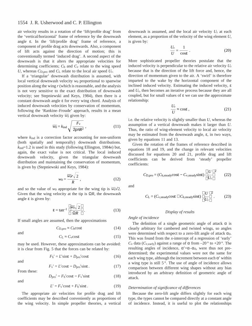
Standard hawkmoth

Fig. 6 shows Ch and Cv plotted against α′ for the standardflat hawkmoth model wing pair. The minimum Ch is notsignificantly different from zero and is, in fact, slightlynegative. This illustrates limits to the accuracy of themeasurements. Significant differences are clear between‘early’ and ‘steady’ values for both vertical and horizontalcoefficients over the mid-range of angles. Maximal values ofCh occur at α′ around 90 °, and Cv peaks between 40 and 50 °.The error bars shown (± 1 S.E.M.) are representative for all wingtypes.

In Figs 7–9, standard hawkmoth results are included as anunderlying grey line and represent 0 ° twist and 0 % camber.

Leading-edge range

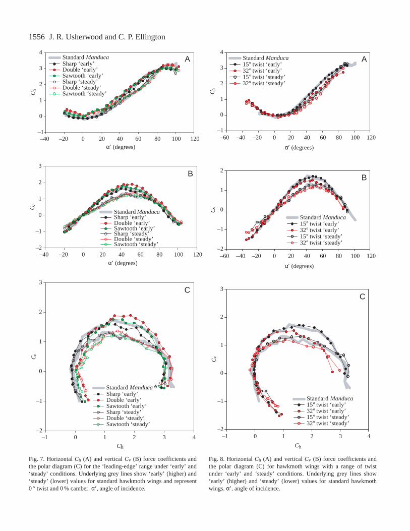
Fig. 7 shows Ch and Cv plotted against α′ for hawkmothwing models with a range of leading-edge forms. Therelationships between force coefficients and α′ are strikinglysimilar, especially for the ‘steady’ values (as might be expectedfrom the greater averaging period). The scatter visible in thepolar diagram (Fig. 7C) incorporates errors in both Ch and Cv,making the scatter more apparent than in Fig. 7A,B.

Twist range

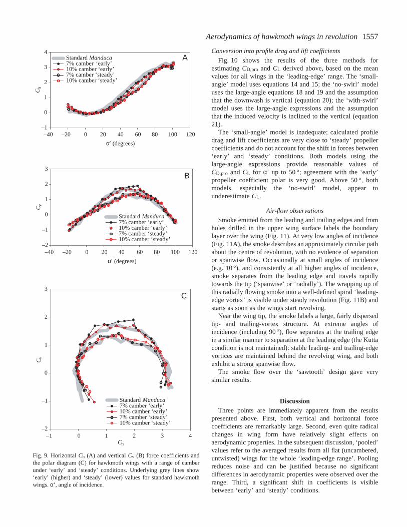
Fig. 8 shows Ch and Cv plotted against α′ for twistedhawkmoth wing models. Results for the 15 ° twist are notsignificantly different from those for the standard flat model.For the 32 ° twist, however, Ch and Cv plotted against α′ bothdecrease under ‘early’ and ‘steady’ conditions at moderate tolarge angles of incidence. This is emphasised in the polardiagram (Fig. 8C), which shows that the maximum forcecoefficients for the 32 ° twist are lower than for the less twistedwings. The degree of shift between ‘early’ and ‘steady’ forcecoefficients is not influenced by twist.

Camber range

Fig. 9 shows Ch and Cv plotted against α′ for cambered

hawkmoth wing models, and the corresponding polar diagramsare presented in Fig. 9C. Consistent differences, if present, arevery slight.

α′ (degrees)

–40 –20 0 20 40 60 80 100 120

Ch

–1

0

1

2

3

4Ch,earlyCh,steady

α′ (degrees)

–40 –20 0 20 40 60 80 100 120

Cv

–2

–1

0

1

2Cv,earlyCv,steady

Ch

–1 0 1 2 3 4

Cv

–2

–1

0

1

2

3

‘Early’‘Steady’

A

B

C

Fig. 6. Horizontal Ch (A) and vertical Cv (B) force coefficients andthe polar diagram (C) for standard hawkmoth wings under ‘early’and ‘steady’ conditions. Error bars in A and B show ±1 S.E.M.,N=4–10. α′ , angle of incidence.

1556 J. R. Usherwood and C. P. Ellington

α′ (degrees) –40 –20 0 20 40 60 80 100 120

Ch

–1

0

1

2

3

4

Sharp ‘early’Double ‘early’Sawtooth ‘early’Sharp ‘steady’Double ‘steady’Sawtooth ‘steady’

α′ (degrees)

–40 –20 0 20 40 60 80 100 120

C v

–2

–1

0

1

2

3

Standard ManducaSharp ‘early’Double ‘early’Sawtooth ‘early’Sharp ‘steady’Double ‘steady’Sawtooth ‘steady’

Ch

–1 0 1 2 3 4

C v

–2

–1

0

1

2

3

Sharp ‘early’Double ‘early’Sawtooth ‘early’Sharp ‘steady’Double ‘steady’Sawtooth ‘steady’

A

B

C

Standard Manduca

Standard Manduca

Fig. 7. Horizontal Ch (A) and vertical Cv (B) force coefficients andthe polar diagram (C) for the ‘leading-edge’ range under ‘early’ and‘steady’ conditions. Underlying grey lines show ‘early’ (higher) and‘steady’ (lower) values for standard hawkmoth wings and represent0 ° twist and 0 % camber. α′ , angle of incidence.

α′ (degrees)

–60 –40 –20 200 40 60 80 100 120

Ch

–1

0

1

2

3

4Standard Manduca15° twist ‘early’32° twist ‘early’15° twist ‘steady’32° twist ‘steady’

α′ (degrees)

–60 –40 –20 200 40 60 80 100 120

Cv

–2

–1

0

1

2

Standard Manduca15° twist ‘early’32° twist ‘early’15° twist ‘steady’32° twist ‘steady’

Ch

–1 0 1 2 3 4

Cv

–2

–1

0

1

2

3

Standard Manduca15° twist ‘early’32° twist ‘early’15° twist ‘steady’32° twist ‘steady’

A

B

C

Fig. 8. Horizontal Ch (A) and vertical Cv (B) force coefficients andthe polar diagram (C) for hawkmoth wings with a range of twistunder ‘early’ and ‘steady’ conditions. Underlying grey lines show‘early’ (higher) and ‘steady’ (lower) values for standard hawkmothwings. α′ , angle of incidence.

1557Aerodynamics of hawkmoth wings in revolution

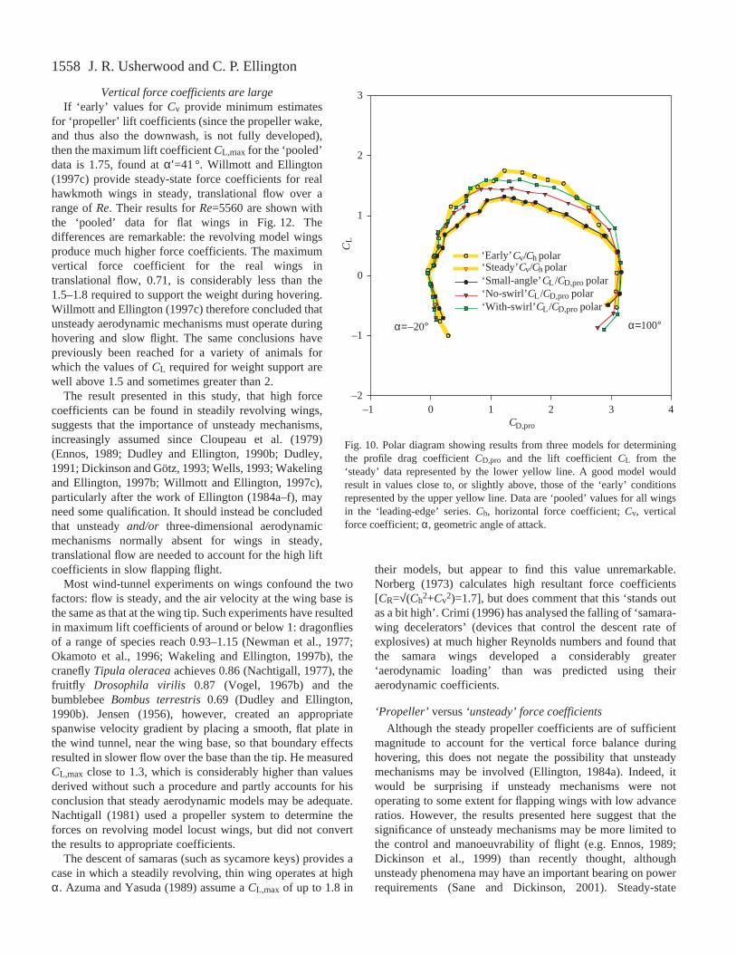
Conversion into profile drag and lift coefficients

Fig. 10 shows the results of the three methods forestimating CD,pro and CL derived above, based on the meanvalues for all wings in the ‘leading-edge’ range. The ‘small-angle’ model uses equations 14 and 15; the ‘no-swirl’ modeluses the large-angle equations 18 and 19 and the assumptionthat the downwash is vertical (equation 20); the ‘with-swirl’model uses the large-angle expressions and the assumptionthat the induced velocity is inclined to the vertical (equation21).

The ‘small-angle’ model is inadequate; calculated profiledrag and lift coefficients are very close to ‘steady’ propellercoefficients and do not account for the shift in forces between‘early’ and ‘steady’ conditions. Both models using thelarge-angle expressions provide reasonable values ofCD,pro and CL for α′ up to 50 °; agreement with the ‘early’propeller coefficient polar is very good. Above 50 °, bothmodels, especially the ‘no-swirl’ model, appear tounderestimate CL.

Air-flow observations

Smoke emitted from the leading and trailing edges and fromholes drilled in the upper wing surface labels the boundarylayer over the wing (Fig. 11). At very low angles of incidence(Fig. 11A), the smoke describes an approximately circular pathabout the centre of revolution, with no evidence of separationor spanwise flow. Occasionally at small angles of incidence(e.g. 10 °), and consistently at all higher angles of incidence,smoke separates from the leading edge and travels rapidlytowards the tip (‘spanwise’ or ‘radially’). The wrapping up ofthis radially flowing smoke into a well-defined spiral ‘leading-edge vortex’ is visible under steady revolution (Fig. 11B) andstarts as soon as the wings start revolving.

Near the wing tip, the smoke labels a large, fairly dispersedtip- and trailing-vortex structure. At extreme angles ofincidence (including 90 °), flow separates at the trailing edgein a similar manner to separation at the leading edge (the Kuttacondition is not maintained): stable leading- and trailing-edgevortices are maintained behind the revolving wing, and bothexhibit a strong spanwise flow.

The smoke flow over the ‘sawtooth’ design gave verysimilar results.

DiscussionThree points are immediately apparent from the results

presented above. First, both vertical and horizontal forcecoefficients are remarkably large. Second, even quite radicalchanges in wing form have relatively slight effects onaerodynamic properties. In the subsequent discussion, ‘pooled’values refer to the averaged results from all flat (uncambered,untwisted) wings for the whole ‘leading-edge range’. Poolingreduces noise and can be justified because no significantdifferences in aerodynamic properties were observed over therange. Third, a significant shift in coefficients is visiblebetween ‘early’ and ‘steady’ conditions.

α′ (degrees)

–40 –20 0 20 40 60 80 100 120

Ch

–1

0

1

2

3

4Standard Manduca7% camber ‘early’10% camber ‘early’7% camber ‘steady’10% camber ‘steady’

α′ (degrees)

–40 –20 0 20 40 60 80 100 120

Cv

–2

–1

0

1

2

3

Standard Manduca7% camber ‘early’10% camber ‘early’7% camber ‘steady’10% camber ‘steady’

Ch

–1 0 1 2 3 4

Cv

–2

–1

0

1

2

3

Standard Manduca7% camber ‘early’10% camber ‘early’7% camber ‘steady’10% camber ‘steady’

A

B

C

Fig. 9. Horizontal Ch (A) and vertical Cv (B) force coefficients andthe polar diagram (C) for hawkmoth wings with a range of camberunder ‘early’ and ‘steady’ conditions. Underlying grey lines show‘early’ (higher) and ‘steady’ (lower) values for standard hawkmothwings. α′ , angle of incidence.

1558

Vertical force coefficients are largeIf ‘early’ values for Cv provide minimum estimates

for ‘propeller’ lift coefficients (since the propeller wake,and thus also the downwash, is not fully developed),then the maximum lift coefficient CL,max for the ‘pooled’data is 1.75, found at α′=41 °. Willmott and Ellington(1997c) provide steady-state force coefficients for realhawkmoth wings in steady, translational flow over arange of Re. Their results for Re=5560 are shown withthe ‘pooled’ data for flat wings in Fig. 12. Thedifferences are remarkable: the revolving model wingsproduce much higher force coefficients. The maximumvertical force coefficient for the real wings intranslational flow, 0.71, is considerably less than the1.5–1.8 required to support the weight during hovering.Willmott and Ellington (1997c) therefore concluded thatunsteady aerodynamic mechanisms must operate duringhovering and slow flight. The same conclusions havepreviously been reached for a variety of animals forwhich the values of CL required for weight support arewell above 1.5 and sometimes greater than 2.

The result presented in this study, that high forcecoefficients can be found in steadily revolving wings,suggests that the importance of unsteady mechanisms,increasingly assumed since Cloupeau et al. (1979)(Ennos, 1989; Dudley and Ellington, 1990b; Dudley,1991; Dickinson and Götz, 1993; Wells, 1993; Wakelingand Ellington, 1997b; Willmott and Ellington, 1997c),particularly after the work of Ellington (1984a–f), mayneed some qualification. It should instead be concludedthat unsteady and/or three-dimensional aerodynamicmechanisms normally absent for wings in steady,translational flow are needed to account for the high liftcoefficients in slow flapping flight.

Most wind-tunnel experiments on wings confound the twofactors: flow is steady, and the air velocity at the wing base isthe same as that at the wing tip. Such experiments have resultedin maximum lift coefficients of around or below 1: dragonfliesof a range of species reach 0.93–1.15 (Newman et al., 1977;Okamoto et al., 1996; Wakeling and Ellington, 1997b), thecranefly Tipula oleraceaachieves 0.86 (Nachtigall, 1977), thefruitfly Drosophila virilis 0.87 (Vogel, 1967b) and thebumblebee Bombus terrestris0.69 (Dudley and Ellington,1990b). Jensen (1956), however, created an appropriatespanwise velocity gradient by placing a smooth, flat plate inthe wind tunnel, near the wing base, so that boundary effectsresulted in slower flow over the base than the tip. He measuredCL,max close to 1.3, which is considerably higher than valuesderived without such a procedure and partly accounts for hisconclusion that steady aerodynamic models may be adequate.Nachtigall (1981) used a propeller system to determine theforces on revolving model locust wings, but did not convertthe results to appropriate coefficients.

The descent of samaras (such as sycamore keys) provides acase in which a steadily revolving, thin wing operates at highα. Azuma and Yasuda (1989) assume a CL,max of up to 1.8 in

their models, but appear to find this value unremarkable.Norberg (1973) calculates high resultant force coefficients[CR=√(Ch2+Cv2)=1.7], but does comment that this ‘stands outas a bit high’. Crimi (1996) has analysed the falling of ‘samara-wing decelerators’ (devices that control the descent rate ofexplosives) at much higher Reynolds numbers and found thatthe samara wings developed a considerably greater‘aerodynamic loading’ than was predicted using theiraerodynamic coefficients.

‘Propeller’ versus‘unsteady’ force coefficients

Although the steady propeller coefficients are of sufficientmagnitude to account for the vertical force balance duringhovering, this does not negate the possibility that unsteadymechanisms may be involved (Ellington, 1984a). Indeed, itwould be surprising if unsteady mechanisms were notoperating to some extent for flapping wings with low advanceratios. However, the results presented here suggest that thesignificance of unsteady mechanisms may be more limited tothe control and manoeuvrability of flight (e.g. Ennos, 1989;Dickinson et al., 1999) than recently thought, althoughunsteady phenomena may have an important bearing on powerrequirements (Sane and Dickinson, 2001). Steady-state

J. R. Usherwood and C. P. Ellington

CD,pro

–1 0 1 2 3 4

CL

–2

–1

0

1

2

3

‘Steady’ Cv/Ch polarCv/Ch polar

‘Small -angle’ CL /CD,pro polar‘No-swirl’ CL /CD,pro polar‘With-swirl’ CL /CD,pro polar

α= –20° α= 100°

‘Early’

Fig. 10. Polar diagram showing results from three models for determiningthe profile drag coefficient CD,pro and the lift coefficient CL from the‘steady’ data represented by the lower yellow line. A good model wouldresult in values close to, or slightly above, those of the ‘early’ conditionsrepresented by the upper yellow line. Data are ‘pooled’ values for all wingsin the ‘leading-edge’ series. Ch, horizontal force coefficient; Cv, verticalforce coefficient; α, geometric angle of attack.

1559Aerodynamics of hawkmoth wings in revolution

‘propeller’ coefficients (derived from revolving wings) may gomuch of the way towards accounting for the lift and powerrequirements of hovering and, while missing unsteady aspects,present the best opportunity for analysing power requirementsin those insects, and those flight sequences, in which finekinematic details are unknown.

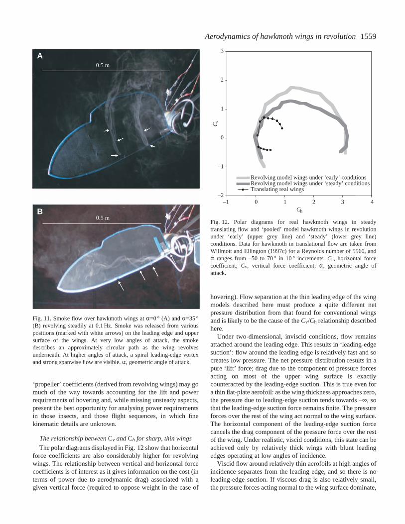
The relationship between Cv and Ch for sharp, thin wings

The polar diagrams displayed in Fig. 12 show that horizontalforce coefficients are also considerably higher for revolvingwings. The relationship between vertical and horizontal forcecoefficients is of interest as it gives information on the cost (interms of power due to aerodynamic drag) associated with agiven vertical force (required to oppose weight in the case of

hovering). Flow separation at the thin leading edge of the wingmodels described here must produce a quite different netpressure distribution from that found for conventional wingsand is likely to be the cause of the Cv/Ch relationship describedhere.

Under two-dimensional, inviscid conditions, flow remainsattached around the leading edge. This results in ‘leading-edgesuction’: flow around the leading edge is relatively fast and socreates low pressure. The net pressure distribution results in apure ‘lift’ force; drag due to the component of pressure forcesacting on most of the upper wing surface is exactlycounteracted by the leading-edge suction. This is true even fora thin flat-plate aerofoil: as the wing thickness approaches zero,the pressure due to leading-edge suction tends towards –∞, sothat the leading-edge suction force remains finite. The pressureforces over the rest of the wing act normal to the wing surface.The horizontal component of the leading-edge suction forcecancels the drag component of the pressure force over the restof the wing. Under realistic, viscid conditions, this state can beachieved only by relatively thick wings with blunt leadingedges operating at low angles of incidence.

Viscid flow around relatively thin aerofoils at high angles ofincidence separates from the leading edge, and so there is noleading-edge suction. If viscous drag is also relatively small,the pressure forces acting normal to the wing surface dominate,

A

B

0.5 m

0.5 m

Fig. 11. Smoke flow over hawkmoth wings at α=0 ° (A) and α=35 °(B) revolving steadily at 0.1 Hz. Smoke was released from variouspositions (marked with white arrows) on the leading edge and uppersurface of the wings. At very low angles of attack, the smokedescribes an approximately circular path as the wing revolvesunderneath. At higher angles of attack, a spiral leading-edge vortexand strong spanwise flow are visible.α, geometric angle of attack.

Ch

–1 0 1 2 3 4

Cv

–2

–1

0

1

2

3

Revolving model wings under ‘early’ conditionsRevolving model wings under ‘steady’ conditionsTranslating real wings

Fig. 12. Polar diagrams for real hawkmoth wings in steadytranslating flow and ‘pooled’ model hawkmoth wings in revolutionunder ‘early’ (upper grey line) and ‘steady’ (lower grey line)conditions. Data for hawkmoth in translational flow are taken fromWillmott and Ellington (1997c) for a Reynolds number of 5560, andα ranges from –50 to 70 ° in 10 ° increments. Ch, horizontal forcecoefficient; Cv, vertical force coefficient; α, geometric angle ofattack.

1560

so the resultant force is perpendicular to the wing surface andnot to the relative velocity. In the case of wings in revolution,the high vertical force coefficients can be attributed to theformation of leading-edge vortices. Leading-edge vortices area result of leading-edge separation and so are directlyassociated with a loss of leading-edge suction; high vertical (orlift) forces due to leading-edge vortices must inevitably resultin high horizontal (or drag) forces (Polhamus, 1971).

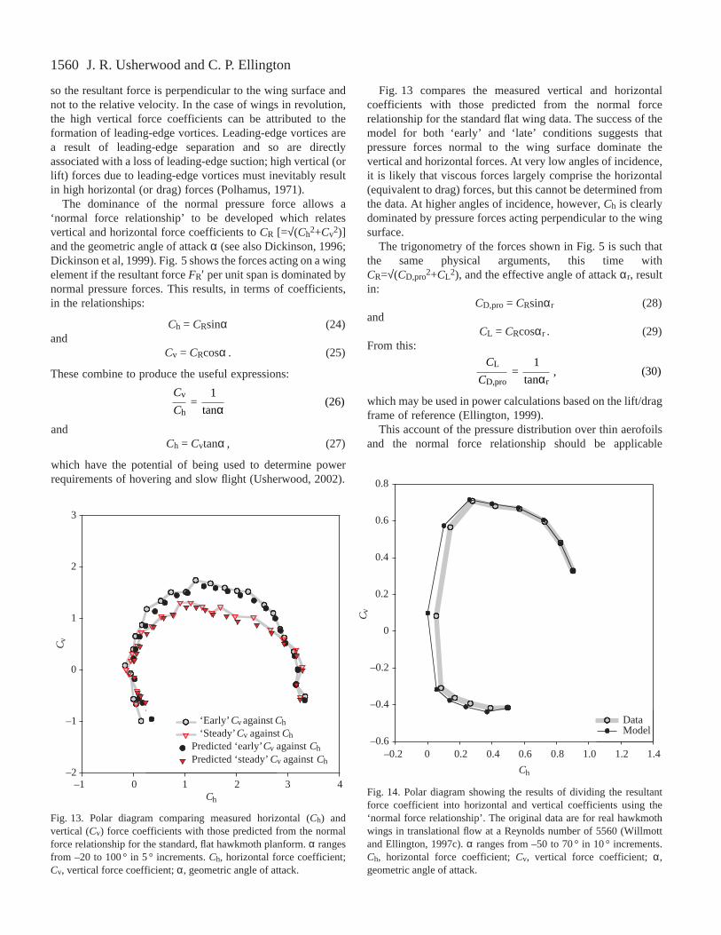
The dominance of the normal pressure force allows a‘normal force relationship’ to be developed which relatesvertical and horizontal force coefficients to CR [=√(Ch2+Cv2)]and the geometric angle of attack α (see also Dickinson, 1996;Dickinson et al, 1999). Fig. 5 shows the forces acting on a wingelement if the resultant force FR′ per unit span is dominated bynormal pressure forces. This results, in terms of coefficients,in the relationships:

Ch = CRsinα (24)and

Cv = CRcosα . (25)

These combine to produce the useful expressions:

andCh = Cvtanα , (27)

which have the potential of being used to determine powerrequirements of hovering and slow flight (Usherwood, 2002).

Fig. 13 compares the measured vertical and horizontalcoefficients with those predicted from the normal forcerelationship for the standard flat wing data. The success of themodel for both ‘early’ and ‘late’ conditions suggests thatpressure forces normal to the wing surface dominate thevertical and horizontal forces. At very low angles of incidence,it is likely that viscous forces largely comprise the horizontal(equivalent to drag) forces, but this cannot be determined fromthe data. At higher angles of incidence, however, Ch is clearlydominated by pressure forces acting perpendicular to the wingsurface.

The trigonometry of the forces shown in Fig. 5 is such thatthe same physical arguments, this time withCR=√(CD,pro2+CL2), and the effective angle of attack αr, resultin:

CD,pro = CRsinαr (28)and

CL = CRcosαr . (29)From this:

which may be used in power calculations based on the lift/dragframe of reference (Ellington, 1999).

This account of the pressure distribution over thin aerofoilsand the normal force relationship should be applicable

(30)1

tanαr

CL

CD,pro= ,

(26)1

tanαCv

Ch=

J. R. Usherwood and C. P. Ellington

Fig. 13. Polar diagram comparing measured horizontal (Ch) andvertical (Cv) force coefficients with those predicted from the normalforce relationship for the standard, flat hawkmoth planform. α rangesfrom –20 to 100 ° in 5 ° increments. Ch, horizontal force coefficient;Cv, vertical force coefficient; α, geometric angle of attack.

Ch

–1 0 1 2 3 4

Cv

–2

–1

0

1

2

3

‘Early’ Cv against Ch

‘Steady’ Cv against Ch

Predicted ‘early’ Cv against Ch

Predicted ‘steady’ Cv against Ch

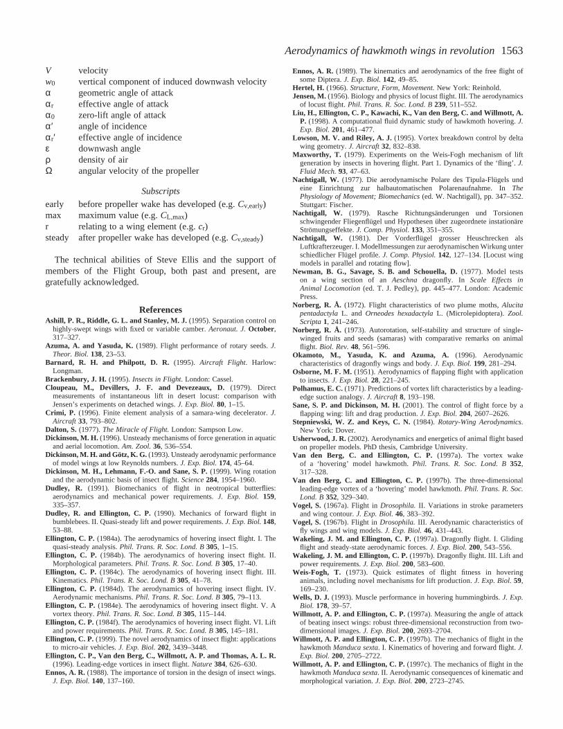
Fig. 14. Polar diagram showing the results of dividing the resultantforce coefficient into horizontal and vertical coefficients using the‘normal force relationship’. The original data are for real hawkmothwings in translational flow at a Reynolds number of 5560 (Willmottand Ellington, 1997c). α ranges from –50 to 70 ° in 10 ° increments.Ch, horizontal force coefficient; Cv, vertical force coefficient; α,geometric angle of attack.

Ch

–0.2 0 0.2 0.4 0.6 0.8 1.0 1.2 1.4

Cv

–0.6

–0.4

–0.2

0

0.2

0.4

0.6

0.8

DataModel

1561Aerodynamics of hawkmoth wings in revolution

whenever the flow separates from a sharp leading edge. Indeed,Fig. 14 shows that the division into vertical and horizontalforce components using equations 24 and 25 fits very well forthe real hawkmoth wings in translating flow, for which theleading-edge vortex is two-dimensional and unstable (Willmottand Ellington, 1997c). The model underestimates Ch at smallangles of attack, but that is simply because skin friction isneglected. However, hawkmoth wings typically operate atmuch higher angles, at which the model fits the data very wellfor both translating and revolving wings.

The effects and implications of wing design

Leading-edge detail

The production of higher coefficients than would be expectedin translating flow appears remarkably robust and is relativelyconsistent over quite a dramatic range of leading-edge styles.This may be surprising because the leading-edge characteristicsof swept or delta wings are known to have effects on leading-edge vortex properties (Lowson and Riley, 1995) and are evenused to delay or control the occurrence of leading-edge vorticesat high angles of incidence. Wing features of some animals,such as the projecting bat thumb or the bird alula, may performsome role in leading-edge vortex delay or control analogous towing fences and vortilons on swept-wing aircraft (see Barnardand Philpott, 1995). Such aircraft wings, and perhaps theanalogous vertebrate wings, experience both conventional(attached) and detached (with a leading-edge vortex) flowregimes at different times and positions along the wing.However, the results presented here suggest that it is unlikelythat very small-scale detail of leading edges, such as theserrations on the leading edges of dragonfly wings (e.g. Hertel,1966), would influence the force coefficients for rapidlyrevolving wings. The peculiar microstructure of dragonflywings may be more closely associated with their exceptionalgliding performance (Wakeling and Ellington, 1997a).

Twist

The ‘early’ and ‘steady’ polar diagrams for the hawkmothwing design with moderate (15 °) twist are virtually identicalto those for the flat wing design (Fig. 8). The only differenceis that the zero-lift angle α0 was approximately –10 ° for thetwisted wing, so angles of incidence α′ ranged from –30 to 90 °instead of –20 to 100 ° as for the flat wings. Thus, the bottomleft of the polar diagram was slightly extended and the bottomright shortened. The effect was even more pronounced for thehighly twisted (32 °) wing design. This design also showed asubstantial reduction in the magnitude of the force coefficientsat high angles of incidence, but this is readily explained: evenwhen the wing base is set to a high angle of incidence, the tipof a highly twisted wing will be at a much lower angle.

Twist is desirable in propeller blades and has been assumedto be desirable for insects by analogy. The downwash angle εis typically smaller towards the faster-moving tip of a propeller,so a lower angle of incidence α′ is needed to give the sameeffective angle of incidence αr′ (=α′–ε). Thus, a twisted bladeallows some optimal effective angle of incidence to be

maintained at each radial station despite the varying effects ofdownwash. However, what this optimal effective angle ofincidence should be is unclear for insects. These revolving, low-Rewings show no features of conventional stall; changes fromhigh Cv to high Ch with increasing angle of incidence can berelated entirely to the normal pressure force and not to thesudden development of a stalled wake. So it is not, presumably,stall that is being avoided with the twisted wing.

The characteristic normally optimised in propeller design isthe ‘aerodynamic efficiency’ or lift-to-drag ratio. This occursat αr′ well below 10 ° for conventional propellers and at α(≈αr′ at these small angles) around 10 ° for the translatinghawkmoth wings (Willmott and Ellington, 1997c). Themaximum lift-to-drag ratio could not be determined in thisstudy because of noise in the torque transducer at small anglesof incidence, but it is reasonable to suppose that the optimalαr′ for aerodynamic efficiency is low, probably below 10 °.This is certainly below the angles used by hawkmoths, inwhich α ranges from 21 to 74 ° (Willmott and Ellington,1997b) or by many hovering insects: Ellington (1984c) givesα=35 ° as a typical value. So, twist is not maintaining an αr′along the wing that maximises the lift-to-drag ratio. Theangles of attack for hovering insects suggest that acompromise between high lift and a reasonably small dragmight be more important than maximising the lift-to-dragratio. They operate near the upper left corner of the polardiagram, and the observed moderate wing twists might sustainthe appropriate αr′ along the wing. However, it must beemphasised that the polar diagrams for the flat and moderatelytwisted wings were almost identical. The same point on thepolar diagram could be attained by either wing design simplyby altering the geometric angle of attack, so there are no clearbenefits to the twisted wing.

Less direct aerodynamic functions of twist should also beconsidered. Ennos (1988) shows that camber may be producedthrough wing twist in many wing designs, so any aerodynamicadvantages of camber might drive the evolution of twistedwings. It is also possible that twisting may have noaerodynamic role whatever or may even be aerodynamicallydisadvantageous. The null hypothesis for this discussionshould be that wing twist is just a structural inevitability forultra-light wings experiencing rapidly changing aerodynamicand inertial forces. Twist may simply occur as a result ofrotational inertia during pronation and supination and bemaintained because of aerodynamic loading on a slightlyflimsy wing. The lack of twist in flapping Drosophila wingshas been explained by the higher relative torsional stiffness ofsmaller wings (Ellington, 1984c). If twisting had aerodynamicadvantages, the evolution of more flexible materials (which, ifanything, should be less costly) might be expected. Of course,these arguments are confounded in many aspects, including Re.However, it is difficult for any description of an aerodynamicfunction of twist to account for the purpose of wings twistedin the opposite sense, where the base operates at lower α thanthe tip. This appears to be the case for Phormia regina(Nachtigall, 1979).

1562

Camber

Fig. 9 agrees with results on the performance of two-dimensional model Drosophila wings in unsteady flow(Dickinson and Götz, 1993); any changes in the aerodynamicproperties of model hawkmoth wings due to camber are slight.Shifts in maximum Ch or Cv appear to be within theexperimental error, so these trends should not be put down toaerodynamic effects. The similarities of the polar diagramsshow that camber provides little improvement in lift-to-dragratios at relevant angles of incidence.

Camber is beneficial in conventional wings because itincreases the angle of incidence gradually across the chord.This shape deflects air downwards gradually, and the abruptand undesirable breaking away of flow from the upper surfaceis avoided. So, the conventional reasoning behind the benefitsof cambered wings to insects appears flawed: flapping insectwings use flow separation at the leading edge as a fundamentalpart of lift generation. A reasonable analogy exists withaeroplane wings. The thin wings of a landing Tornado jet useleading- and trailing-edge flaps to increase wing camber,maintaining attached flow and allowing higher lift coefficientsthan would otherwise be possible. Concorde, however, uses thehigh force coefficients associated with leading-edge vorticescreated by flow separation from the sharp, swept leading edges:no conventional leading-edge flaps are used because flowseparation from the leading edge is intentional.

Camber still has a role in improving the aerodynamicperformance of gliding wings, but any beneficial aerodynamiceffects for flapping insect wings will require experimentalevidence and not analogy with conventional wings designed(or adapted) for attached flow.

Accounting for differences between ‘early’ and ‘steady’propeller coefficients

Fig. 4 and Figs 6–9 show that there is a considerable changein force production between ‘early’ and ‘steady’ conditions.There are two possible reasons for this change. First, the wingscause an induced flow in steady revolution that is absent at thestart, and this decreases the effective angle of incidence.Second, there may be a fundamental change in aerodynamicsdue, for instance, to the shedding of the leading-edge vortex(and a resulting stall), as is seen for translating wings(Dickinson and Götz, 1993). Simple accounts are taken of theinduced downwash in the calculation of CD,pro and CL fromsteady coefficients (Fig. 10). Below α′=50 °, the downwashalone appears to account for the shift between ‘early’ and‘steady’ propeller coefficients; the calculated values of CD,pro

and CL fit the observed values of Ch,earlyand Cv,earlywell. Also,the observation (Fig. 11) that leading-edge vortices can bemaintained during steady revolution supports the view that theshift in propeller coefficients can be accounted for by theeffects of downwash alone, without a fundamental change inaerodynamics.

At very high α′ , the downwash models for determiningCD,pro and CL provide poorer results. A change in the value ofw0— at high α′ can improve the fit of CD,pro and CL to Ch,early

and Cv,early: both kind and R (separation at the wing tip mayreduce the effective wing length) in equation 11 may bealtered. However, varying correction factors in the high α′range without a priori justification (such as more accurate flowvisualisation) limits the possibility of aerodynamic inferences.Both fundamental changes in aerodynamics and failure of theRankine–Froude actuator disc model for calculating induceddownwash are also reasonable explanations for part of the shiftin propeller coefficients between ‘early’ and ‘steady’conditions at very high α′ . The appearance of trailing-edgevortices at high angles of incidence may be a relevantaerodynamic shift and may also account for the relatively highforce values for 45 °<α<75 °. An aerodynamic change due toa shift in the position of the vortex core breakdown isparticularly worthy of consideration. Ellington et al. (1996) andVan den Berg and Ellington (1997b) noted that the core of thespiral leading-edge vortex broke down at approximately two-thirds of the wing length, resulting in a loss of lift in outer wingregions. Liu et al. (1998) postulated that this breakdown is dueto the adverse pressure gradient over the upper wing surfacecaused by the tip vortex. The development of the full vortexwake with its associated radial inflow over the wings mightwell shift the position of vortex breakdown inwards under‘steady’ conditions at higher α′ , producing a quantitativereduction in the lift coefficient compared with the ‘early’ state.

List of symbolsAR aspect ratioc wing chordCD,pro profile drag coefficientCh horizontal force coefficientCL lift coefficientCR resultant force coefficientCv vertical force coefficientDpro profile dragDpro′ Profile drag on wing elementFh horizontal forceFh′ Horizontal force on wing elementFv vertical forceFv′ Vertical force on wing elementFR′ single resultant forcekind correction factor for induced powerL liftL′ Lift on wing elementQ torquer radial position along the wingr2(S) non-dimensional second moment of arear3(S) non-dimensional third moment of areaR wing lengthRe Reynolds numberS total wing area (for two wings)S2 second moment of area for both wingsS3 third moment of area for both wingsU velocity of a wing elementUr relative velocity of air at a wing element

J. R. Usherwood and C. P. Ellington

1563Aerodynamics of hawkmoth wings in revolution

V velocityw0 vertical component of induced downwash velocityα geometric angle of attackαr effective angle of attackα0 zero-lift angle of attackα′ angle of incidenceαr′ effective angle of incidenceε downwash angleρ density of airΩ angular velocity of the propeller

Subscripts

early before propeller wake has developed (e.g. Cv,early)max maximum value (e.g. CL,max)r relating to a wing element (e.g. cr)steady after propeller wake has developed (e.g. Cv,steady)

The technical abilities of Steve Ellis and the support ofmembers of the Flight Group, both past and present, aregratefully acknowledged.

ReferencesAshill, P. R., Riddle, G. L. and Stanley, M. J. (1995). Separation control on

highly-swept wings with fixed or variable camber. Aeronaut. J.October,317–327.

Azuma, A. and Yasuda, K.(1989). Flight performance of rotary seeds. J.Theor. Biol. 138, 23–53.

Barnard, R. H. and Philpott, D. R. (1995). Aircraft Flight. Harlow:Longman.

Brackenbury, J. H. (1995). Insects in Flight. London: Cassel.Cloupeau, M., Devillers, J. F. and Devezeaux, D.(1979). Direct

measurements of instantaneous lift in desert locust: comparison withJensen’s experiments on detached wings. J. Exp. Biol.80, 1–15.

Crimi, P. (1996). Finite element analysis of a samara-wing decelerator. J.Aircraft 33, 793–802.

Dalton, S. (1977). The Miracle of Flight.London: Sampson Low.Dickinson, M. H. (1996). Unsteady mechanisms of force generation in aquatic

and aerial locomotion. Am. Zool.36, 536–554.Dickinson, M. H. and Götz, K. G.(1993). Unsteady aerodynamic performance

of model wings at low Reynolds numbers. J. Exp. Biol.174, 45–64.Dickinson, M. H., Lehmann, F.-O. and Sane, S. P.(1999). Wing rotation

and the aerodynamic basis of insect flight. Science 284, 1954–1960.Dudley, R. (1991). Biomechanics of flight in neotropical butterflies:

aerodynamics and mechanical power requirements. J. Exp. Biol. 159,335–357.

Dudley, R. and Ellington, C. P. (1990). Mechanics of forward flight inbumblebees. II. Quasi-steady lift and power requirements. J. Exp. Biol. 148,53–88.

Ellington, C. P. (1984a). The aerodynamics of hovering insect flight. I. Thequasi-steady analysis. Phil. Trans. R. Soc. Lond. B305, 1–15.

Ellington, C. P. (1984b). The aerodynamics of hovering insect flight. II.Morphological parameters. Phil. Trans. R. Soc. Lond. B305, 17–40.

Ellington, C. P. (1984c). The aerodynamics of hovering insect flight. III.Kinematics.Phil. Trans. R. Soc. Lond. B305, 41–78.

Ellington, C. P. (1984d). The aerodynamics of hovering insect flight. IV.Aerodynamic mechanisms. Phil. Trans. R. Soc. Lond. B305, 79–113.

Ellington, C. P. (1984e). The aerodynamics of hovering insect flight. V. Avortex theory. Phil. Trans. R. Soc. Lond. B305, 115–144.

Ellington, C. P. (1984f). The aerodynamics of hovering insect flight. VI. Liftand power requirements. Phil. Trans. R. Soc. Lond. B 305, 145–181.

Ellington, C. P. (1999). The novel aerodynamics of insect flight: applicationsto micro-air vehicles. J. Exp. Biol.202, 3439–3448.

Ellington, C. P., Van den Berg, C., Willmott, A. P. and Thomas, A. L. R.(1996). Leading-edge vortices in insect flight. Nature 384, 626–630.

Ennos, A. R.(1988). The importance of torsion in the design of insect wings.J. Exp. Biol. 140, 137–160.

Ennos, A. R.(1989). The kinematics and aerodynamics of the free flight ofsome Diptera. J. Exp. Biol. 142, 49–85.

Hertel, H. (1966). Structure, Form, Movement.New York: Reinhold.Jensen, M.(1956). Biology and physics of locust flight. III. The aerodynamics

of locust flight. Phil. Trans. R. Soc. Lond. B239, 511–552.Liu, H., Ellington, C. P., Kawachi, K., Van den Berg, C. and Willmott, A.

P. (1998). A computational fluid dynamic study of hawkmoth hovering. J.Exp. Biol. 201, 461–477.

Lowson, M. V. and Riley, A. J.(1995). Vortex breakdown control by deltawing geometry. J. Aircraft 32, 832–838.

Maxworthy, T. (1979). Experiments on the Weis-Fogh mechanism of liftgeneration by insects in hovering flight. Part 1. Dynamics of the ‘fling’. J.Fluid Mech.93, 47–63.

Nachtigall, W. (1977). Die aerodynamische Polare des Tipula-Flügels undeine Einrichtung zur halbautomatischen Polarenaufnahme. In ThePhysiology of Movement; Biomechanics (ed. W. Nachtigall), pp. 347–352.Stuttgart: Fischer.

Nachtigall, W. (1979). Rasche Richtungsänderungen und Torsionenschwingender Fliegenflügel und Hypothesen über zugeordnete instationäreStrömungseffekte. J. Comp. Physiol. 133, 351–355.

Nachtigall, W. (1981). Der Vorderflügel grosser Heuschrecken alsLuftkrafterzeuger. I. Modellmessungen zur aerodynamischen Wirkung unterschiedlicher Flügel profile. J. Comp. Physiol. 142, 127–134. [Locust wingmodels in parallel and rotating flow].

Newman, B. G., Savage, S. B. and Schouella, D.(1977). Model testson a wing section of an Aeschna dragonfly. In Scale Effects inAnimal Locomotion(ed. T. J. Pedley), pp. 445–477. London: AcademicPress.

Norberg, R. Å. (1972). Flight characteristics of two plume moths, AlucitapentadactylaL. and Orneodes hexadactylaL. (Microlepidoptera). Zool.Scripta1, 241–246.

Norberg, R. Å. (1973). Autorotation, self-stability and structure of single-winged fruits and seeds (samaras) with comparative remarks on animalflight. Biol. Rev.48, 561–596.

Okamoto, M., Yasuda, K. and Azuma, A. (1996). Aerodynamiccharacteristics of dragonfly wings and body. J. Exp. Biol.199, 281–294.

Osborne, M. F. M. (1951). Aerodynamics of flapping flight with applicationto insects. J. Exp. Biol.28, 221–245.

Polhamus, E. C.(1971). Predictions of vortex lift characteristics by a leading-edge suction analogy. J. Aircraft 8, 193–198.

Sane, S. P. and Dickinson, M. H.(2001). The control of flight force by aflapping wing: lift and drag production. J. Exp. Biol. 204, 2607–2626.

Stepniewski, W. Z. and Keys, C. N.(1984). Rotary-Wing Aerodynamics.New York: Dover.

Usherwood, J. R. (2002). Aerodynamics and energetics of animal flight basedon propeller models. PhD thesis, Cambridge University.

Van den Berg, C. and Ellington, C. P. (1997a). The vortex wakeof a ‘hovering’ model hawkmoth. Phil. Trans. R. Soc. Lond. B352,317–328.

Van den Berg, C. and Ellington, C. P.(1997b). The three-dimensionalleading-edge vortex of a ‘hovering’ model hawkmoth. Phil. Trans. R. Soc.Lond. B 352, 329–340.

Vogel, S.(1967a). Flight in Drosophila. II. Variations in stroke parametersand wing contour. J. Exp. Biol.46, 383–392.

Vogel, S.(1967b). Flight in Drosophila. III. Aerodynamic characteristics offly wings and wing models. J. Exp. Biol. 46, 431–443.

Wakeling, J. M. and Ellington, C. P. (1997a). Dragonfly flight. I. Glidingflight and steady-state aerodynamic forces. J. Exp. Biol.200, 543–556.

Wakeling, J. M. and Ellington, C. P.(1997b). Dragonfly flight. III. Lift andpower requirements. J. Exp. Biol.200, 583–600.

Weis-Fogh, T. (1973). Quick estimates of flight fitness in hoveringanimals, including novel mechanisms for lift production. J. Exp. Biol. 59,169–230.

Wells, D. J. (1993). Muscle performance in hovering hummingbirds. J. Exp.Biol. 178, 39–57.

Willmott, A. P. and Ellington, C. P. (1997a). Measuring the angle of attackof beating insect wings: robust three-dimensional reconstruction from two-dimensional images. J. Exp. Biol.200, 2693–2704.

Willmott, A. P. and Ellington, C. P. (1997b). The mechanics of flight in thehawkmoth Manduca sexta. I. Kinematics of hovering and forward flight. J.Exp. Biol. 200, 2705–2722.

Willmott, A. P. and Ellington, C. P. (1997c). The mechanics of flight in thehawkmoth Manduca sexta. II. Aerodynamic consequences of kinematic andmorphological variation. J. Exp. Biol. 200, 2723–2745.

1564

Willmott, A. P., Ellington, C. P. and Thomas, A. L. R. (1997). Flowvisualization and unsteady aerodynamics in the flight of the hawkmoth,Manduca sexta. Phil. Trans. R. Soc. Lond. B 352, 303–316.

Wootton, R. J. (1981). Support and deformability in insect wings. J. Zool.,Lond.193, 447–468.

Wootton, R. J. (1991). The functional morphology of the wings of Odonata.Adv. Odonatol.5, 153–169.

Wootton, R. J. (1992). Functional morphology of insect wings. Annu. Rev.Entomol.37, 113–140.

Wootton, R. J. (1993). Leading edge sections and asymmetric twisting in thewings of flying butterflies (Insects, Papilionoidea). J. Exp. Biol. 180,105–117.

Wootton, R. J. (1995). Geometry and mechanics of insect hindwing fans – amodelling approach. Proc. R. Soc. Lond. B262, 181–187.

J. R. Usherwood and C. P. Ellington