The ‘Delta method’ - Montefiore Institutekvansteen/MATH0008-2/ac20122013/Class2Oct... · Appendix B The ‘Delta method’ ... Suppose you have done a study, over 4 years, which

Appendix B

The ‘Delta method’ . . .

Suppose you have done a study, over 4 years, which yields 3 estimates of survival (say, φ1, φ2, and

φ3). But, suppose what you are really interested in is the estimate of the product of the three survival

values (i.e., the probability of surviving from the beginning of the study to the end of the study)?

While it is easy enough to derive an estimate of this product (as [φ1 × φ2 × φ3]), how do you derive

an estimate of the variance of the product? In other words, how do you derive an estimate of the

variance of a transformation of one or more random variables (in this case, we transform the three

random variables - φi - by considering their product)?

One commonly used approach which is easily implemented, not computer-intensive, and can be

robustly applied in many (but not all) situations is the so-called Delta method (also known as the

method of propagation of errors). In this appendix, we briefly introduce the underlying background

theory, and the implementation of the Delta method, to fairly typical scenarios.

B.1. Mean and variance of random variables

Our primary interest here is developing a method that will allow us to estimate the mean and

variance for functions of random variables. Let’s start by considering the formal approach for deriving

these values explicitly, based on the method of moments. For continuous random variables, consider a

continuous function f (x) on the interval [−∞,+∞]. The first three moments of f (x) can be written

as

M0 =∫ +∞

−∞f (x)dx

M1 =∫ +∞

−∞x f (x)dx

M2 =∫ +∞

−∞x2 f (x)dx

In the particular case that the function is a probability density (as for a continuous random variable),

then M0 = 1 (i.e., the area under the PDF must equal 1).

For example, consider the uniform distribution on the finite interval [a, b]. A uniform distribution

(sometimes also known as a rectangular distribution), is a distribution that has constant probability

c© Cooch & White (2012) 05.10.2012

B.1. Mean and variance of random variables B - 2

over the interval. The probability density function (pdf) for a continuous uniform distribution on the

finite interval [a, b] is

P(x) =

0 for x < a

1/(b − a) for a < x < b

0 for x > b

Integrating the pdf, for p(x) = 1/(b − a),

M0 =∫ b

ap(x)dx

=∫ b

a

1

b − adx = 1 (B.1)

M1 =∫ b

axp(x)dx

=∫ b

a

x

b − adx =

a + b

2(B.2)

M2 =∫ b

ax2 p(x)dx

=∫ b

ax2 1

b − adx =

1

3

(a2 + ab + b2

)(B.3)

We see clearly that M1 is the mean of the distribution. What about the variance? Where does

the second moment M2 come in? Recall that the variance is defined as the average value of the

fundamental quantity [distance from mean]2. The squaring of the distance is so the values to either

side of the mean don’t cancel out. Standard deviation is simply the square-root of the variance.

Given some discrete random variable xi, with probability pi, and mean µ, we define the variance

as

Var = ∑ (xi − µ)2 pi

Note we don’t have to divide by the number of values of x because the sum of the discrete probability

distribution is 1 (i.e., ∑ pi = 1). For a continuous probability distribution, with mean µ, we define the

variance as

Var =∫ b

a(x − µ)2 p(x)dx

Given our moment equations, we can then write

Var =∫ b

a(x − µ)2 p(x)dx

=∫ b

a

(x2 − 2µx + µ2

)p(x)dx

=∫ b

ax2 p(x)dx −

∫ b

a2µxp(x)dx +

∫ b

aµ2 p(x)dx

=∫ b

ax2 p(x)dx − 2µ

∫ b

axp(x)dx + µ2

∫ b

ap(x)dx

Now, if we look closely at the last line, we see that in fact the terms represent the different moments

Appendix B. The ‘Delta method’ . . .

B.2. Transformations of random variables and the Delta method B - 3

of the distribution. Thus we can write

Var =∫ b

a(x − µ)2 p(x)dx

=∫ b

ax2 p(x)dx − 2µ

∫ b

axp(x)dx + µ2

∫ b

ap(x)dx

= M2 − 2µ (M1) + µ2 (M0)

Since M1 = µ, and M0 = 1 then

Var = M2 − 2µ (M1) + µ2 (M0)

= M2 − 2µ(µ) + µ2(1)

= M2 − 2µ2 + µ2

= M2 − µ2

= M2 − (M1)2

In other words, the variance for the pdf is simply the second moment (M2) minus the square of the

first moment ((M1)2). Thus, for a continuous uniform random variable x on the interval [a, b],

Var = M2 − (M1)2

=(a − b)2

12

B.2. Transformations of random variables and the Delta

method

OK - that’s fine. If the pdf is specified, we can use the method of moments to formally derive the

mean and variance of the distribution. But, what about functions of random variables having poorly

specified or unspecified distributions? Or, situations where the pdf is not easily defined?

In such cases, we may need other approaches. We’ll introduce one such approach (the Delta

method) here, by considering the case of a simple linear transformation of a random normal dis-

tribution.

Let

X1, X2, . . . ∼ N(10, σ2 = 2)

In other words, random deviates drawn from a normal distribution with a mean of 10, and a variance

of 2. Consider some transformations of these random values. You might recall from some earlier

statistics or probability class that linearly transformed normal random variables are themselves

normally distributed. Consider for example, Xi ∼ N(10, 2) - which we then linearly transform to

Yi, such that Yi = 4Xi + 3.

Now, recall that for real scalar constants a and b we can show that

i. E(a) = a, E(aX + b) = aE(X) + b

ii. var(a) = 0, var(aX + b) = a2var(X)



Thus, given Xi ∼ N(10, 2) and the linear transformation Yi = 4Xi + 3, we can write

Y ∼ N(4(10) + 3 = 43, (42)2) = N(43, 32)

Now, an important point to note is that some transformations of the normal distribution are close to

normal (i.e., are linear) and some are not. Since linear transformations of random normal values are

normal, it seems reasonable to conclude that approximately linear transformations (over some range)

of random normal data should also be approximately normal.

OK, to continue. Let X ∼ N(µ, σ2),and let Y = g(X), where g is some transformation of X (in the

previous example, g(X) = 4X + 3). It is hopefully relatively intuitive that the closer g(X) is to linear

over the likely range of X (i.e., within 3 or so standard deviations of µ), the closer Y = g(X) will be

to normally distributed. From calculus, we recall that if you look at any differentiable function over

a narrow enough region, the function appears approximately linear. The approximating line is the

tangent line to the curve, and it’s slope is the derivative of the function.

Since most of the mass (i.e., most of the random values) of X is concentrated around µ, let’s figure

out the tangent line at µ, using two different methods. First, we know that the tangent line passes

through (µ, g(µ)), and that it’s slope is g′µ (we use the ‘g′’ notation to indicate the first derivative of

the function g). Thus, the equation of the tangent line is Y = g′X + b for some b. Replacing (X, Y) with

the known point (µ, g(µ)), we find g(µ) = g′(µ)µ + b and so b = g(µ)− g′(µ)µ. Thus, the equation

of the tangent line is Y = g′(µ)X + g(µ)− g′(µ)µ.

Now for the big step – we can derive an approximation to the same tangent line by using a Taylor

series expansion of g(x) (to first order) around X = µ

Y = g(X)

≈ g(µ) + g′(µ)(X − u) + ǫ

= g′(µ)X + g(µ)− g′(µ)µ + ǫ

OK, at this point you might be asking yourself ‘so what?’. Well, suppose that X ∼ N(µ, σ2) and

Y = g(X), where g′(µ) 6= 0. Then, whenever the tangent line (derived earlier) is approximately

correct over the likely range of X (i.e., if the transformed function is approximately linear over the

likely range of X), then the transformation Y = g(X) will have an approximate normal distribution.

That approximate normal distribution may be found using the usual rules for linear transformations

of normals.

Thus, to first order,

E(Y) = g′(µ)µ + g(µ)− g′(µ)µ = g(µ)

var(Y) = var(g(X)) = (g(X)− g(µ))2

=(

g′(µ)(X − µ))2

= (g′(µ))2(X − µ)2

= (g′(µ))2var(X)

In other words, we take the derivative of the transformed function with respect to the parameter,

square it, and multiply it by the estimated variance of the untransformed parameter.

These first-order approximations to the variance of a transformed parameter are usually referred

to as the Delta method.



begin sidebar

Taylor series expansions?

A very important, and frequently used tool. If you have no familiarity at all with series expansions,

here is a (very) short introduction. Briefly, the Taylor series is a power series expansion of an infinitely

differentiable real (or complex) function defined on an open interval around some specified point.

For example, a one-dimensional Taylor series is an expansion of a real function f (x) about a point

x = a over the interval (a − r, a + r), is given as:

f (x) ≈ f (a) +f ′(a)(x − a)

1!+

f ′′(x)(x − a)2

2!+ . . .

where f ′(a) is the first derivative of f with respect to a, f ′′(x) is the second derivative of f with

respect to a, and so on.

For example, suppose the function is f (x) = ex . The convenient fact about this function is that

all it’s derivatives are equal to ex as well (i.e., f (x) = ex , f ′(x) = ex, f ′′ = ex, . . .). In particular,

f (n)(x) = ex so that f (n)(0) = 1 . This means that the coefficients of the Taylor series are given by

an =f (n)(0)

n!=

1

n!

and so the Taylor series is given by

1 + x +x2

2+

x3

6+

x4

24+ . . . +

xn

n!+ . . . =

∞

∑n=0

xn

n!

The primary utility of such a power series in simple application is that differentiation and integra-

tion of power series can be performed term by term and is hence particularly (or, at least relatively)

easy. In addition, the (truncated) series can be used to compute function values approximately.

Now, let’s look at an example of the “fit” of a Taylor series to a familiar function, given a certain

number of terms in the series. For our example, we’ll expand the function f (x) = ex , at x = a = 0,

on the interval (a− 2, a+ 2), for n = 0, n = 1, n = 2, . . . (where n is the number of terms in the series).

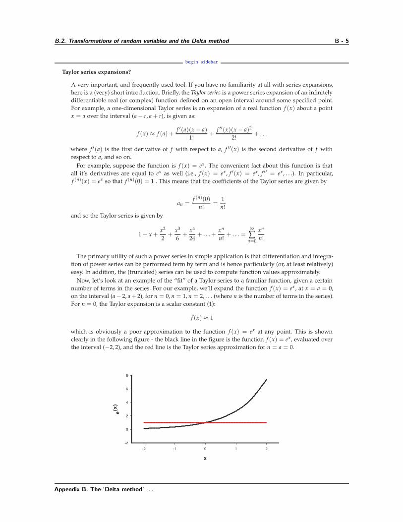
For n = 0, the Taylor expansion is a scalar constant (1):

f (x) ≈ 1

which is obviously a poor approximation to the function f (x) = ex at any point. This is shown

clearly in the following figure - the black line in the figure is the function f (x) = ex, evaluated over

the interval (−2, 2), and the red line is the Taylor series approximation for n = a = 0.



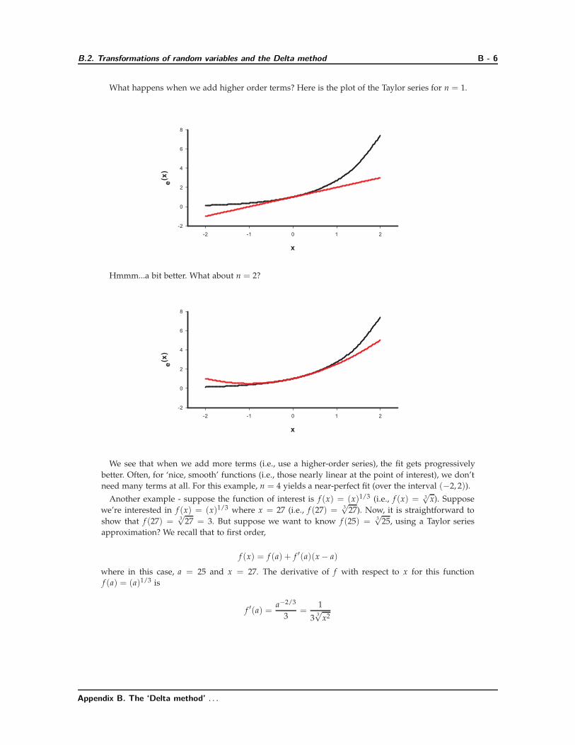
What happens when we add higher order terms? Here is the plot of the Taylor series for n = 1.

Hmmm...a bit better. What about n = 2?

We see that when we add more terms (i.e., use a higher-order series), the fit gets progressively

better. Often, for ‘nice, smooth’ functions (i.e., those nearly linear at the point of interest), we don’t

need many terms at all. For this example, n = 4 yields a near-perfect fit (over the interval (−2, 2)).

Another example - suppose the function of interest is f (x) = (x)1/3 (i.e., f (x) = 3√

x). Suppose

we’re interested in f (x) = (x)1/3 where x = 27 (i.e., f (27) = 3√

27). Now, it is straightforward to

show that f (27) = 3√

27 = 3. But suppose we want to know f (25) = 3√

25, using a Taylor series

approximation? We recall that to first order,

f (x) = f (a) + f ′(a)(x − a)

where in this case, a = 25 and x = 27. The derivative of f with respect to x for this function

f (a) = (a)1/3 is

f ′(a) =a−2/3

3=

1

33√

x2


B.3. Transformations of one variable B - 7

Thus, using the first-order Taylor series, we write

f (25) ≈ f (27) + f ′(27)(25 − 27)

= 3 + (0.037037)(−2)

= 3 − 0.0740741

= 2.926

which is very close to the true value of f (25) = 3√

25 = 2.924. In other words, the first-order Taylor

approximation works pretty well for this function.

end sidebar

B.3. Transformations of one variable

OK, enough background for now. Let’s see some applications. Let’s check the Delta method out in

a case where we know the answer. Assume we have an estimate of density D and it’s conditional

sampling variance, var(Ds). We want to multiply this by some constant c to make it comparable with

other values from the literature. Thus, we want Ds = g(D) = cD and varDs.

The Delta method gives

var(Ds) = (g′(D))2σ2D

=

(∂Ds

∂D

)2

· var(D)

= c2 · var(D)

which we know to be true for the variance of a random variable multiplied by a real constant.

Another example of the same thing – consider a known number of harvested fish and an average

weight (µw) and it’s variance. If you want an estimate of total biomass (B), then B = N · µw and the

variance of B is N2 · var(µw).

Still another example - you have some parameter θ, which you transform by dividing it by some

constant c. Thus, by the Delta method,

var

(θ

c

)=

(1

c

)2

· var(θ)

B.3.1. A potential complication - violation of assumptions

A final - and important - example for transformations of single variables. The importance lies in

the demonstration that the Delta method does not always work - remember, it assumes that the

transformation is approximately linear over the expected range of the parameter. Suppose one has an

MLE for the mean and estimated variance for some parameter θ which is bounded random uniform

on the interval [0, 2]. Suppose you want to transform this parameter such that

ψ = e(θ)


B.3.1. A potential complication - violation of assumptions B - 8

(Recall that this is a convenient transformation since the derivative of ex is ex, making the calculations

very simple). Now, based on the Delta method, the variance for ψ would be estimated as

var(ψ) =

(∂ψ

∂θ

)2

· var(θ)

=(

eθ)2

· var(θ)

Now, suppose that θ = 1.0, and var(θ) = 0.33. Then, from the Delta method,

var(ψ) =(

eθ)2

· var(θ)

= (7.38906)(0.33)

= 2.46302

OK, so what’s the problem? Well, let’s derive the variance of ψ using the method of moments. To

do this, we need to integrate the pdf (uniform, in this case) over some range. Since the variance of a

uniform distribution is (b − a)2/12, and if b and a are symmetric around the mean (1.0), then we can

show by algebra that given a variance of 0.33, then a = 0 and b = 2.

Given a uniform distribution, the pdf is p(θ) = 1/(b − a). Thus, by the method of moments,

M1 =∫ b

ag(x)p(x)dx

=∫ b

a

g(x)

b − adx

= − eb − ea

a − b

M2 =∫ b

a

g(x)2

b − adx

=1

2

e2a − e2b

a − b

Thus, by moments, var(E(ψ) is

var(E(ψ)) = M2 − (M1)2 =

1

2

−e2b + e2a

−b + a−

(eb − ea

)2

(a − b)2

If a = 0 and b = 2, then

var(E(ψ)) = M2 − (M1)2 =

1

2

−e2b + e2a

−b + a−

(eb − ea

)2

(a − b)2= 3.19453

which is not particularly close to the value estimated by the Delta method (2.46302).

Why the discrepancy? As discussed earlier, the Delta method rests on the assumption the first-

order Taylor expansion around the parameter value is effectively linear over the range of values likely


B.3.1. A potential complication - violation of assumptions B - 9

to be encountered. Since in this example we’re using a uniform pdf, then all values between a and b

are equally likely. Thus, we might anticipate that as the interval between a and b gets smaller, then

the approximation to the variance (which will clearly decrease) will get better and better (since the

smaller the interval, the more likely it is that the function is approximately linear over that range).

For example, if a = 0.5 and b = 1.5 (same mean of 1.0), then the true variance of θ will be 0.083. Thus,

by the Delta method, the estimated variance of ψ will be 0.61575, while by the method of moments

(which is exact), the variance will be 0.65792. Clearly, the proportional difference between the two

values has declined markedly. But, we achieved this ’improvement’ by artificially reducing the true

variance of the untransformed variable θ. Obviously, we can’t do this in general practice.

So, what are the practical options? Well, one possible solution is to use a higher-order Taylor series

approximation - by including higher-order terms, we can achieve a better ’fit’ to the function (see the

preceding sidebar). If we used a second-order TSE,

E(g(x)) ≈ g(µ) +1

2g′′(µ)σ2 (B.4)

Var(g(x)) ≈ g′(µ)2σ2 +1

4(g′′(µ))2(Var(x2)− 4µ2σ2) (B.5)

we should do a bit better. For the variance estimate, we need to know var(x2), which for a continuous

uniform distribution by the method of moments is

(1

5· b5 − a5

b − a

)−(

1

9·(b3 − a3

)2

(b − a)2

)

Thus, from the second-order approximation, and again assuming a = 0 and b = 2, then var(ψ)) is

var(ψ)) ≈ (eθ)2 · var(θ) +1

4(eθ)2 · var(θ2)− 4µ2var(θ)

= 3.756316

which is closer (proportionately) to the true variance (3.19453) than was the estimate using only the

first-order TSE (2.46302). The reason that even a second-order approximation isn’t ‘much closer’ is

because the transformation is very non-linear over the range of the data (uniform [0, 2] in this case),

such that the second-order approximation doesn’t ‘fit’ particularly well over this range.

So, we see that the classical Delta method, which is based on a first-order Taylor series expansion

of the transformed function, may not do particularly well if the function is highly non-linear over the

range of values being examined.

Of course, it would be fair to note that the preceding example made the assumption that the

distribution was random uniform over the interval. For most of our work with MARK, the interval

is likely to have a symmetric mass around the estimate, typically β. As such, most of data, and

thus the transformed data, will actually fall closer to the parameter value in question (the mean

in this example) than we’ve demonstrated here. So much so, that the discrepancy between the

first order ‘Delta’ approximation to the variance and the true value of the variance will likely be

significantly smaller than shown here, even for a strongly non-linear transformation. We leave it

to you as an exercise to prove this for yourself. But, this point notwithstanding, it is important to

be aware of the assumptions underlying the Delta method - if your transformation is non-linear,

and there is considerable variation in your data, the first-order approximation may not be particular

good. Fortunately, use of second order Taylor series approximations is not heroically difficult – the

challenge is usually coming up with var(X2). If the pdf for the untransformed data is specified (which


B.4. Transformations of two or more variables B - 10

is essentially equivalent to assuming an informative prior), then you can derive var(X2) fairly easily

using the method of moments.

B.4. Transformations of two or more variables

Clearly, we are often interested in transformations involving more than one variable. Fortunately,

there are also multivariate generalizations of the Delta method.

Suppose you’ve estimated p different random variables X1, X2, . . . , Xp. In matrix notation, these

variables would constitute a (p × 1) random vector

X =

X1

X2

...

Xp

which has a mean vector

µ =

EX1

EX2

...

EXp

=

µ1

µ2

...

µp

and the (p × p) variance-covariance matrix is

var(X1) cov(X1, X2) . . . cov(X1, Xp)

cov(X2, X1) var(X2) . . . cov(X2, Xp)

......

......

cov(Xp, X1) cov(Xp, X2) . . . var(Xp)

Note that if the variables are independent, then the off-diagonal elements (i.e., the covariance terms)

are all zero.

Then, for a (k × p) matrix of constants A = aij, the expectation of a random vector Y = AX is given

as

EY1

EY2

...

EYp

= Aµ

with a variance-covariance matrix

cov(Y) = AΣAT



Now, using the same logic we first considered for developing the Delta method for a single variable,

for each xi near µi, we can write

y =

g1(x)

g2(x)

...

gp(x)

≈

g1(µ)

g2(µ)

...

gp(µ)

+ D(x − µ)

where D is the matrix of partial derivatives of gi with respect to xj, evaluated at (x − µ).

As with the single-variable Delta method, if the variances of the Xi are small (so that with high

probability Y is near µ, such that the linear approximation is usually valid), then to first-order we can

write

EY1

EY2

...

EYp

=

g1(µ)

g2(µ)

...

gp(µ)

var(Y) ≈ DΣDT

In other words, to approximate the variance of some multi-variable function Y, we (i) take the vector

of partial derivatives of the function with respect to each parameter in turn, D, (ii) right-multiply

this vector by the variance-covariance matrix, Σ, and (iii) right-multiply the resulting product by the

transpose of the original vector of partial derivatives, DT.∗

Example (1) - variance of product of survival probabilities

Let’s consider the application of the Delta method in estimating sampling variances of a fairly

common function - the product of several parameter estimates.

Now, from the preceding, we see that

var(Y) ≈ DΣDT =

(∂(Y)

∂(θ)

)· Σ ·

(∂(Y)

∂(θ)

)T

where Y is some linear or nonlinear function of the parameter estimates θ1, θ2, . . . . The first term on

the RHS of the variance expression is a row vector containing partial derivatives of Y with respect

∗ There are alternative formulations of this expression which may be more convenient to implement in some instances. Whenthe variables θ1, θ2 . . . θk (in the function, Y) are independent, then

var(Y) ≈ var( f (θ1, θ2, . . . θk))

=k

∑i=1

var(θi)

(∂ f

∂θi

)2

where ∂ f /∂θ1 is the partial derivative of Y with respect to θi .

When the variables θ1 , θ2 . . . θk (in the function, Y) are not independent, then the covariance structure among the variablesmust be accounted for:

var(Y) ≈ var( f (θ1, θ2 , . . . θk))

=k

∑i=1

var(θi)

(∂ f

∂θi

)2

+ 2k

∑i=1

k

∑j=1

cov(θi, θj)

(∂ f

∂θi

)(∂ f

∂θj

)



to each of these parameters (θ1, θ2, . . .). The right-most term of the RHS of the variance expression is

simply a transpose of this row vector (i.e., a column vector). The middle-term is simply the estimated

variance-covariance matrix for the parameters.

OK, let’s try an example - let’s use estimates from the male European dipper data set (yes, again).

We’ll fit model {φt p.} to these data. Suppose we’re interested in the probability of surviving from the

start of the first interval to the end of the third interval. Well, the point-estimate of this probability

is easy enough - it’s simply(φ1 × φ2 × φ3

)= (0.6109350× 0.458263× 0.4960239) = 0.138871. So, the

probability of a male Dipper surviving over the first three intervals is ∼ 14% (again, assuming that

our time-dependent survival model is a valid model).

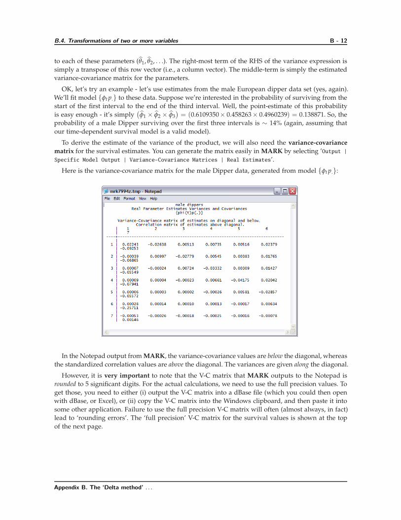
To derive the estimate of the variance of the product, we will also need the variance-covariance

matrix for the survival estimates. You can generate the matrix easily in MARK by selecting ’Output |

Specific Model Output | VarianceCovariance Matrices | Real Estimates’.

Here is the variance-covariance matrix for the male Dipper data, generated from model {φt p.}:

In the Notepad output from MARK, the variance-covariance values are below the diagonal, whereas

the standardized correlation values are above the diagonal. The variances are given along the diagonal.

However, it is very important to note that the V-C matrix that MARK outputs to the Notepad is

rounded to 5 significant digits. For the actual calculations, we need to use the full precision values. To

get those, you need to either (i) output the V-C matrix into a dBase file (which you could then open

with dBase, or Excel), or (ii) copy the V-C matrix into the Windows clipboard, and then paste it into

some other application. Failure to use the full precision V-C matrix will often (almost always, in fact)

lead to ‘rounding errors’. The ‘full precision’ V-C matrix for the survival values is shown at the top

of the next page.



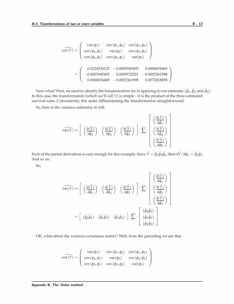
cov(Y) =

var(φ1) cov(φ1, φ2) cov(φ1, φ3)

cov(φ2, φ1) var(φ2) cov(φ2, φ3)

cov(φ3, φ1) cov(φ3, φ2) var(φ3)

=

0.0224330125 −0.0003945405 0.0000654469

−0.0003945405 0.0099722201 −0.0002361998

0.0000654469 −0.0002361998 0.0072418858

Now what? First, we need to identify the transformation we’re applying to our estimates(φ1, φ2, and φ3

).

In this case, the transformation (which we’ll call Y) is simple - it is the product of the three estimated

survival rates. Conveniently, this make differentiating the transformation straightforward.

So, here is the variance estimator, in full:

var(Y) ≈[ (

∂(Y)∂φ1

) (∂(Y)∂φ2

) (∂(Y)∂φ3

) ]· ∑ ·

(∂(Y)∂φ1

)

(∂(Y)∂φ2

)

(∂(Y)∂φ3

)

Each of the partial derivatives is easy enough for this example. Since Y = φ1φ2φ3, then ∂Y/∂φ1 = φ2φ3.

And so on.

So,

var(Y) ≈[ (

∂(Y)∂φ1

) (∂(Y)∂φ2

) (∂(Y)∂φ3

) ]· ∑ ·

(∂(Y)∂φ1

)

(∂(Y)∂φ2

)

(∂(Y)∂φ3

)

=[ (

φ2φ3

) (φ1φ3

) (φ1φ2

) ] · ∑ ·

(φ2φ3

)(φ1φ3

)(φ1φ2

)

OK, what about the variance-covariance matrix? Well, from the preceding we see that

cov(Y) =






=

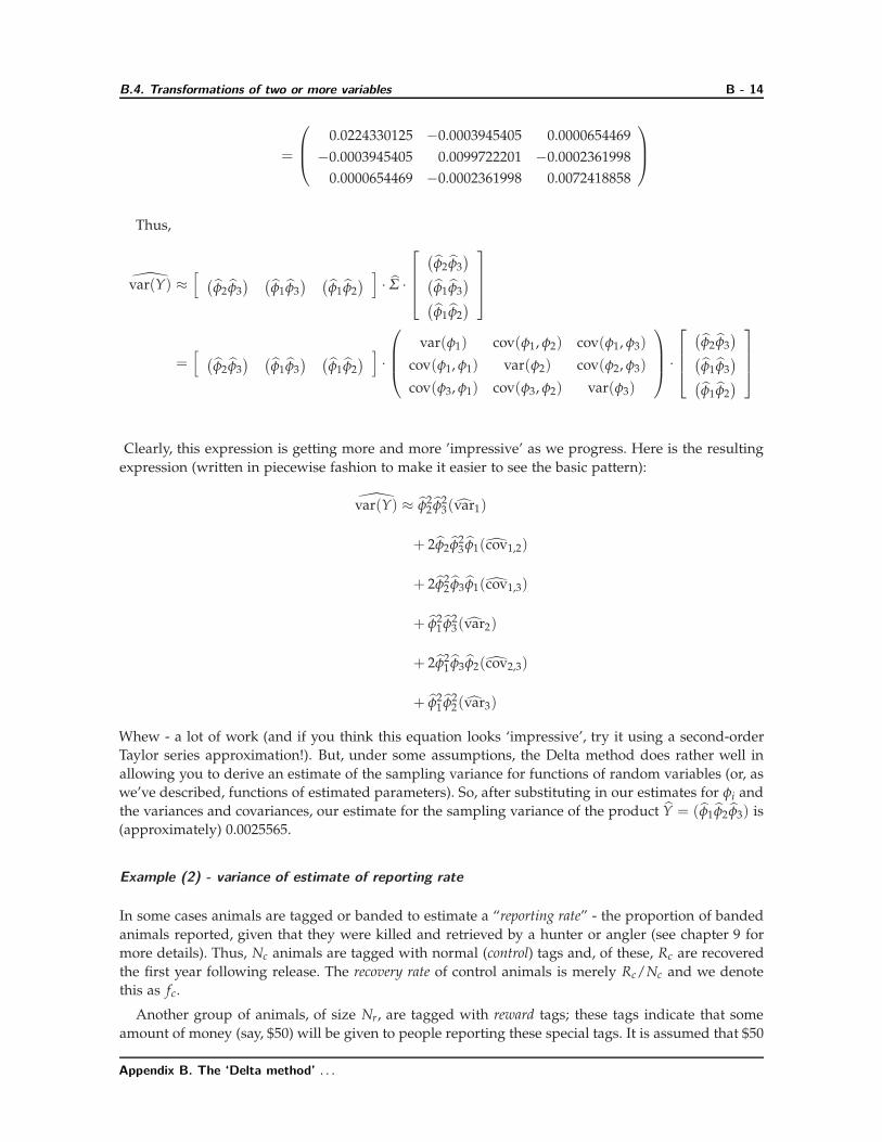
0.0224330125 −0.0003945405 0.0000654469

−0.0003945405 0.0099722201 −0.0002361998

0.0000654469 −0.0002361998 0.0072418858

Thus,

var(Y) ≈[ (

φ2φ3

) (φ1φ3

) (φ1φ2

) ] · Σ ·

(φ2φ3

)(φ1φ3

)(φ1φ2

)

=[ (

φ2φ3

) (φ1φ3

) (φ1φ2

) ] ·




·

(φ2φ3

)(φ1φ3

)(φ1φ2

)

Clearly, this expression is getting more and more ’impressive’ as we progress. Here is the resulting

expression (written in piecewise fashion to make it easier to see the basic pattern):

var(Y) ≈ φ22φ2

3(var1)

+ 2φ2φ23 φ1(cov1,2)

+ 2φ22 φ3φ1(cov1,3)

+ φ21 φ2

3(var2)

+ 2φ21 φ3φ2(cov2,3)

+ φ21 φ2

2(var3)

Whew - a lot of work (and if you think this equation looks ‘impressive’, try it using a second-order

Taylor series approximation!). But, under some assumptions, the Delta method does rather well in

allowing you to derive an estimate of the sampling variance for functions of random variables (or, as

we’ve described, functions of estimated parameters). So, after substituting in our estimates for φi and

the variances and covariances, our estimate for the sampling variance of the product Y = (φ1φ2φ3) is

(approximately) 0.0025565.

Example (2) - variance of estimate of reporting rate

In some cases animals are tagged or banded to estimate a “reporting rate” - the proportion of banded

animals reported, given that they were killed and retrieved by a hunter or angler (see chapter 9 for

more details). Thus, Nc animals are tagged with normal (control) tags and, of these, Rc are recovered

the first year following release. The recovery rate of control animals is merely Rc/Nc and we denote

this as fc.

Another group of animals, of size Nr, are tagged with reward tags; these tags indicate that some

amount of money (say, $50) will be given to people reporting these special tags. It is assumed that $50



is sufficient to ensure that all such tags will be reported, thus these serve as a basis for comparison and

the estimation of a reporting rate. The recovery probability for the reward tagged animals is merely

Rr/Nr, where Rr is the number of recoveries of reward-tagged animals the first year following release.

We denote this recovery probability as fr.

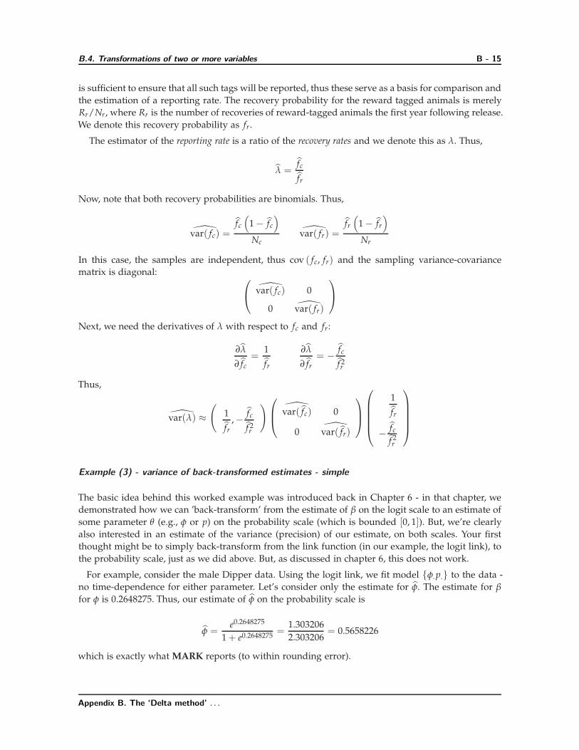
The estimator of the reporting rate is a ratio of the recovery rates and we denote this as λ. Thus,

λ =fc

fr

Now, note that both recovery probabilities are binomials. Thus,

var( fc) =fc

(1 − fc

)

Ncvar( fr) =

fr

(1 − fr

)

Nr

In this case, the samples are independent, thus cov ( fc, fr) and the sampling variance-covariance

matrix is diagonal: var( fc) 0

0 var( fr)

Next, we need the derivatives of λ with respect to fc and fr:

∂λ

∂ fc

=1

fr

∂λ

∂ fr

= − fc

f 2r

Thus,

var(λ) ≈(

1

fr

,− fc

f 2r

)

var( fc) 0

0 var( fr)

1

fr

− fc

f 2r

Example (3) - variance of back-transformed estimates - simple

The basic idea behind this worked example was introduced back in Chapter 6 - in that chapter, we

demonstrated how we can ’back-transform’ from the estimate of β on the logit scale to an estimate of

some parameter θ (e.g., φ or p) on the probability scale (which is bounded [0, 1]). But, we’re clearly

also interested in an estimate of the variance (precision) of our estimate, on both scales. Your first

thought might be to simply back-transform from the link function (in our example, the logit link), to

the probability scale, just as we did above. But, as discussed in chapter 6, this does not work.

For example, consider the male Dipper data. Using the logit link, we fit model {φ. p.} to the data -

no time-dependence for either parameter. Let’s consider only the estimate for φ. The estimate for β

for φ is 0.2648275. Thus, our estimate of φ on the probability scale is

φ =e0.2648275

1 + e0.2648275=

1.303206

2.303206= 0.5658226

which is exactly what MARK reports (to within rounding error).



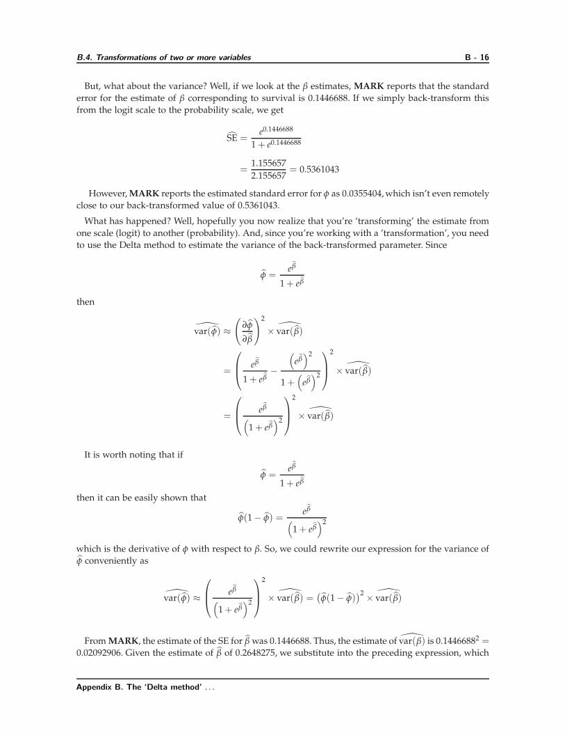
But, what about the variance? Well, if we look at the β estimates, MARK reports that the standard

error for the estimate of β corresponding to survival is 0.1446688. If we simply back-transform this

from the logit scale to the probability scale, we get

SE =e0.1446688

1 + e0.1446688

=1.155657

2.155657= 0.5361043

However, MARK reports the estimated standard error for φ as 0.0355404, which isn’t even remotely

close to our back-transformed value of 0.5361043.

What has happened? Well, hopefully you now realize that you’re ‘transforming’ the estimate from

one scale (logit) to another (probability). And, since you’re working with a ’transformation’, you need

to use the Delta method to estimate the variance of the back-transformed parameter. Since

φ =eβ

1 + eβ

then

var(φ) ≈(

∂φ

∂β

)2

× var(β)

=

eβ

1 + eβ−

(eβ)2

1 +(

eβ)2

2

× var(β)

=

eβ

(1 + eβ

)2

2

× var(β)

It is worth noting that if

φ =eβ

1 + eβ

then it can be easily shown that

φ(1 − φ) =eβ

(1 + eβ

)2

which is the derivative of φ with respect to β. So, we could rewrite our expression for the variance of

φ conveniently as

var(φ) ≈

eβ

(1 + eβ

)2

2

× var(β) =(φ(1 − φ)

)2 × var(β)

From MARK, the estimate of the SE for β was 0.1446688. Thus, the estimate of var(β) is 0.14466882 =0.02092906. Given the estimate of β of 0.2648275, we substitute into the preceding expression, which



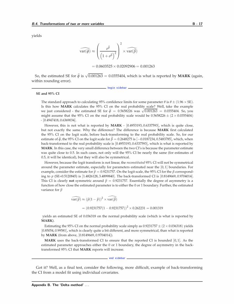
yields

var(φ) ≈

eβ

(1 + eβ

)2

2

× var(β)

= 0.0603525× 0.02092906 = 0.001263

So, the estimated SE for φ is√

0.001263 = 0.0355404, which is what is reported by MARK (again,

within rounding error).

begin sidebar

SE and 95% CI

The standard approach to calculating 95% confidence limits for some parameter θ is θ ± (1.96 × SE).

Is this how MARK calculates the 95% CI on the real probability scale? Well, take the example

we just considered - the estimated SE for φ = 0.5658226 was√

0.001263 = 0.0355404. So, you

might assume that the 95% CI on the real probability scale would be 0.5658226 ± (2 × 0.0355404)

- [0.4947418, 0.6369034].

However, this is not what is reported by MARK - [0.4953193, 0.6337593], which is quite close,

but not exactly the same. Why the difference? The difference is because MARK first calculated

the 95% CI on the logit scale, before back-transforming to the real probability scale. So, for our

estimate of φ, the 95% CI on the logit scale for β = 0.2648275 is [−0.0187234, 0.5483785], which, when

back-transformed to the real probability scale is [0.4953193, 0.6337593], which is what is reported by

MARK. In this case, the very small difference between the two CI’s is because the parameter estimate

was quite close to 0.5. In such cases, not only will the 95% CI be nearly the same (for estimates of

0.5, it will be identical), but they will also be symmetrical.

However, because the logit transform is not linear, the reconstituted 95% CI will not be symmetrical

around the parameter estimate, especially for parameters estimated near the [0, 1] boundaries. For

example, consider the estimate for p = 0.9231757. On the logit scale, the 95% CI for the β correspond-

ing to p (SE=0.5120845) is [1.4826128, 3.4899840]. The back-transformed CI is [0.8149669, 0.9704014].

This CI is clearly not symmetric around p = 0.9231757. Essentially the degree of asymmetry is a

function of how close the estimated parameter is to either the 0 or 1 boundary. Further, the estimated

variance for p

var( p) ≈ ( p(1 − p))2 × var(β)

= (0.9231757(1 − 0.9231757))2 × 0.262231 = 0.001319

yields an estimated SE of 0.036318 on the normal probability scale (which is what is reported by

MARK).

Estimating the 95% CI on the normal probability scale simply as 0.9231757 ± (2× 0.036318) yields

[0.85054, 0.99581], which is clearly quite a bit different, and more symmetrical, than what is reported

by MARK (from above, [0.8149669, 0.9704014]).

MARK uses the back-transformed CI to ensure that the reported CI is bounded [0, 1]. As the

estimated parameter approaches either the 0 or 1 boundary, the degree of asymmetry in the back-

transformed 95% CI that MARK reports will increase.

end sidebar

Got it? Well, as a final test, consider the following, more difficult, example of back-transforming

the CI from a model fit using individual covariates.



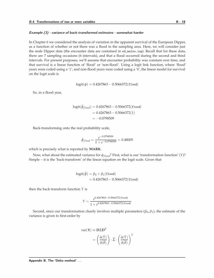
Example (3) - variance of back-transformed estimates - somewhat harder

In Chapter 6 we considered the analysis of variation in the apparent survival of the European Dipper,

as a function of whether or not there was a flood in the sampling area. Here, we will consider just

the male Dipper data (the encounter data are contained in ed_males.inp). Recall that for these data,

there are 7 sampling occasions (6 intervals), and that a flood occurred during the second and third

intervals. For present purposes, we’ll assume that encounter probability was constant over time, and

that survival is a linear function of ‘flood’ or ‘non-flood’. Using a logit link function, where ‘flood’

years were coded using a ‘1’, and non-flood years were coded using a ‘0’, the linear model for survival

on the logit scale is

logit(φ) = 0.4267863− 0.5066372(flood)

So, in a flood year,

logit(φ f lood) = 0.4267863− 0.5066372(flood)

= 0.4267863− 0.5066372(1)

= −0.0798509

Back-transforming onto the real probability scale,

φ f lood =e−0.0798509

1 + e−0.0798509= 0.48005

which is precisely what is reported by MARK.

Now, what about the estimated variance for φ f lood? First, what is our ‘transformation function’ (Y)?

Simple – it is the ‘back-transform’ of the linear equation on the logit scale. Given that

logit(φ) = β0 + β1(flood)

= 0.4267863− 0.5066372(flood)

then the back-transform function Y is

Y =e0.4267863−0.5066372(flood)

1 + e0.4267863−0.5066372(flood)

Second, since our transformation clearly involves multiple parameters (β0, β1), the estimate of the

variance is given to first-order by

var(Y) ≈ DΣDT

=

(∂(Y)

∂(θ)

)· Σ ·

(∂(Y)

∂(θ)

)T



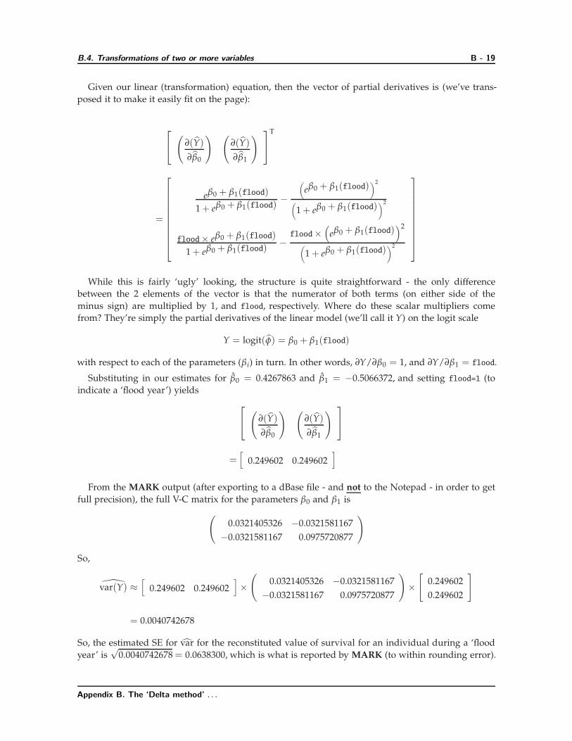
Given our linear (transformation) equation, then the vector of partial derivatives is (we’ve trans-

posed it to make it easily fit on the page):

(

∂(Y)

∂β0

) (∂(Y)

∂β1

)

T

=

eβ0 + β1(flood)

1 + eβ0 + β1(flood)−

(eβ0 + β1(flood)

)2

(1 + eβ0 + β1(flood)

)2

flood× eβ0 + β1(flood)

1 + eβ0 + β1(flood)−

flood×(

eβ0 + β1(flood))2

(1 + eβ0 + β1(flood)

)2

While this is fairly ‘ugly’ looking, the structure is quite straightforward - the only difference

between the 2 elements of the vector is that the numerator of both terms (on either side of the

minus sign) are multiplied by 1, and flood, respectively. Where do these scalar multipliers come

from? They’re simply the partial derivatives of the linear model (we’ll call it Y) on the logit scale

Y = logit(φ) = β0 + β1(flood)

with respect to each of the parameters (βi) in turn. In other words, ∂Y/∂β0 = 1, and ∂Y/∂β1 = flood.

Substituting in our estimates for β0 = 0.4267863 and β1 = −0.5066372, and setting flood=1 (to

indicate a ‘flood year’) yields

(

∂(Y)

∂β0

) (∂(Y)

∂β1

)

=[

0.249602 0.249602]

From the MARK output (after exporting to a dBase file - and not to the Notepad - in order to get

full precision), the full V-C matrix for the parameters β0 and β1 is

(0.0321405326 −0.0321581167

−0.0321581167 0.0975720877

)

So,

var(Y) ≈[

0.249602 0.249602]×(

0.0321405326 −0.0321581167

−0.0321581167 0.0975720877

)×[

0.249602

0.249602

]

= 0.0040742678

So, the estimated SE for var for the reconstituted value of survival for an individual during a ‘flood

year’ is√

0.0040742678 = 0.0638300, which is what is reported by MARK (to within rounding error).



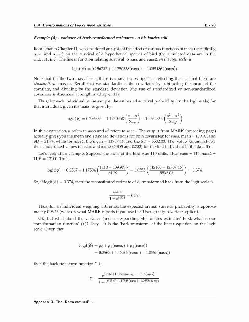
Example (4) - variance of back-transformed estimates - a bit harder still

Recall that in Chapter 11, we considered analysis of the effect of various functions of mass (specifically,

mass, and mass2) on the survival of a hypothetical species of bird (the simulated data are in file

indcov1.inp). The linear function relating survival to mass and mass2, on the logit scale, is

logit(φ) = 0.256732+ 1.1750358(masss)− 1.0554864(mass2s )

Note that for the two mass terms, there is a small subscript ‘s’ - reflecting the fact that these are

‘standardized’ masses. Recall that we standardized the covariates by subtracting the mean of the

covariate, and dividing by the standard deviation (the use of standardized or non-standardized

covariates is discussed at length in Chapter 11).

Thus, for each individual in the sample, the estimated survival probability (on the logit scale) for

that individual, given it’s mass, is given by

logit(φ) = 0.256732+ 1.1750358

(m− m

SDm

)− 1.0554864

(m2 − m2

SDm2

)

In this expression, m refers to mass and m2 refers to mass2. The output from MARK (preceding page)

actually gives you the mean and standard deviations for both covariates: for mass, mean = 109.97, and

SD = 24.79, while for mass2, the mean = 12707.46, and the SD = 5532.03. The ‘value’ column shows

the standardized values for mass and mass2 (0.803 and 0.752) for the first individual in the data file.

Let’s look at an example. Suppose the mass of the bird was 110 units. Thus mass = 110, mass2 =

1102 = 12100. Thus,

logit(φ) = 0.2567+ 1.17504

((110− 109.97)

24.79

)− 1.0555

((12100− 12707.46)

5532.03

)= 0.374.

So, if logit(φ) = 0.374, then the reconstituted estimate of φ, transformed back from the logit scale is

e0.374

1 + e0.374= 0.592

Thus, for an individual weighing 110 units, the expected annual survival probability is approxi-

mately 0.5925 (which is what MARK reports if you use the ’User specify covariate’ option).

OK, but what about the variance (and corresponding SE) for this estimate? First, what is our

‘transformation function’ (Y)? Easy - it is the ‘back-transform’ of the linear equation on the logit

scale. Given that

logit(φ) = β0 + β1(masss) + β2(mass2s )

= 0.2567+ 1.17505(masss)− 1.0555(mass2s )

then the back-transform function Y is

Y =e0.2567+1.17505(masss)−1.0555(mass2

s )

1 + e0.2567+1.17505(masss)−1.0555(mass2s )



As in the preceding example, since our transformation clearly involves multiple parameters

(β0, β1, β2), the estimate of the variance is given by

var(Y) ≈ DΣDT

=

(∂(Y)

∂(θ)

)· Σ ·

(∂(Y)

∂(θ)

)T

Given our linear (transformation) equation (from above) then the vector of partial derivatives is

(we’ve substituted m for mass and m2 for mass2, and transposed it to make it easily fit on the page):

(

∂(Y)

∂β0

) (∂(Y)

∂β1

) (∂(Y)

∂β2

)

T

=

eβ0 + β1(m) + β2(m2)

1 + eβ0 + β1(m) + β2(m2)−

(eβ0 + β1(m) + β2(m2)

)2

(1 + eβ0 + β1(m) + β2(m2)

)2

m× eβ0 + β1(m) + β2(m2)

1 + eβ0 + β1(m) + β2(m2)−

m×(

eβ0 + β1(m) + β2(m2))2

(1 + eβ0 + β1(m) + β2(m2)

)2

m2× eβ0 + β1(m) + β2(m2)

1 + eβ0 + β1(m) + β2(m2)−

m2×(

eβ0 + β1(m) + β2(m2))2

(1 + eβ0 + β1(m) + β2(m2)

)2

Again, while this is fairly ‘ugly’ looking (even more so than the previous example), the structure

is again quite straightforward – the only difference between the 3 elements of the vector is that the

numerator of both terms (on either side of the minus sign) are multiplied by 1, m, and m2, respectively,

which are simply the partial derivatives of the linear model (we’ll call it Y) on the logit scale

Y = logit(φ) = β0 + β1(ms) + β2(m2s )

with respect to each of the parameters (βi) in turn. In other words, ∂Y/∂β0 = 1, ∂Y/∂β1 = m, and

∂Y/∂β2 = m2.

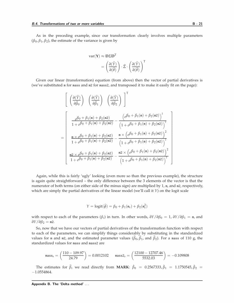
So, now that we have our vectors of partial derivatives of the transformation function with respect

to each of the parameters, we can simplify things considerably by substituting in the standardized

values for m and m2, and the estimated parameter values (β0, β1, and β2). For a mass of 110 g, the

standardized values for mass and mass2 are

masss =

(110− 109.97

24.79

)= 0.0012102 mass2s =

(12100− 12707.46

5532.03

)= −0.109808

The estimates for βi we read directly from MARK: β0 = 0.2567333, β1 = 1.1750545, β2 =−1.0554864.



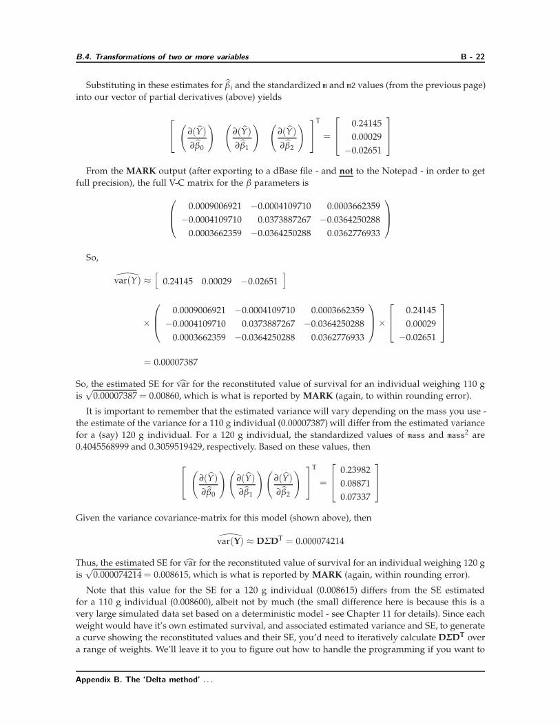
Substituting in these estimates for βi and the standardized m and m2 values (from the previous page)

into our vector of partial derivatives (above) yields

(

∂(Y)

∂β0

) (∂(Y)

∂β1

) (∂(Y)

∂β2

)

T

=

0.24145

0.00029

−0.02651

From the MARK output (after exporting to a dBase file - and not to the Notepad - in order to get

full precision), the full V-C matrix for the β parameters is

0.0009006921 −0.0004109710 0.0003662359

−0.0004109710 0.0373887267 −0.0364250288

0.0003662359 −0.0364250288 0.0362776933

So,

var(Y) ≈[

0.24145 0.00029 −0.02651]

×

0.0009006921 −0.0004109710 0.0003662359

−0.0004109710 0.0373887267 −0.0364250288

0.0003662359 −0.0364250288 0.0362776933

×

0.24145

0.00029

−0.02651

= 0.00007387

So, the estimated SE for var for the reconstituted value of survival for an individual weighing 110 g

is√

0.00007387 = 0.00860, which is what is reported by MARK (again, to within rounding error).

It is important to remember that the estimated variance will vary depending on the mass you use -

the estimate of the variance for a 110 g individual (0.00007387) will differ from the estimated variance

for a (say) 120 g individual. For a 120 g individual, the standardized values of mass and mass2 are

0.4045568999 and 0.3059519429, respectively. Based on these values, then

(

∂(Y)

∂β0

)(∂(Y)

∂β1

)(∂(Y)

∂β2

)

T

=

0.23982

0.08871

0.07337

Given the variance covariance-matrix for this model (shown above), then

var(Y) ≈ DΣDT = 0.000074214

Thus, the estimated SE for var for the reconstituted value of survival for an individual weighing 120 g

is√

0.000074214 = 0.008615, which is what is reported by MARK (again, within rounding error).

Note that this value for the SE for a 120 g individual (0.008615) differs from the SE estimated

for a 110 g individual (0.008600), albeit not by much (the small difference here is because this is a

very large simulated data set based on a deterministic model - see Chapter 11 for details). Since each

weight would have it’s own estimated survival, and associated estimated variance and SE, to generate

a curve showing the reconstituted values and their SE, you’d need to iteratively calculate DΣDT over

a range of weights. We’ll leave it to you to figure out how to handle the programming if you want to


B.5. Delta method and model averaging B - 23

do this on your own. For the less ambitious, MARK now has the capacity to do much of this for you

- you can output the 95% CI ‘data’ over a range of individual covariate values to a spreadsheet (see

section 11.5 in Chapter 11).

B.5. Delta method and model averaging

In the preceding examples, we focused on the application of the Delta method to transformations

of parameter estimates from a single model. However, as introduced in Chapter 4 - and emphasized

throughout the remainder of this book - we’re often interested in accounting for model selection

uncertainty by using model-averaged values. There is no major complication for application of the

Delta method to model-averaged parameter values - you simply need to make sure you use model-

averaged values for each element of the calculations.

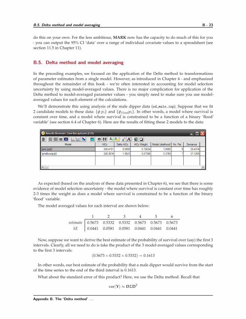
We’ll demonstrate this using analysis of the male dipper data (ed_male.inp). Suppose that we fit

2 candidate models to these data: {φ. pt} and {φ f loodpt}. In other words, a model where survival is

constant over time, and a model where survival is constrained to be a function of a binary ‘flood’

variable’ (see section 6.4 of Chapter 6). Here are the results of fitting these 2 models to the data:

As expected (based on the analysis of these data presented in Chapter 6), we see that there is some

evidence of model selection uncertainty - the model where survival is constant over time has roughly

2-3 times the weight as does a model where survival is constrained to be a function of the binary

‘flood’ variable.

The model averaged values for each interval are shown below:

1 2 3 4 5 6

estimate 0.5673 0.5332 0.5332 0.5673 0.5673 0.5673

SE 0.0441 0.0581 0.0581 0.0441 0.0441 0.0441

Now, suppose we want to derive the best estimate of the probability of survival over (say) the first 3

intervals. Clearly, all we need to do is take the product of the 3 model-averaged values corresponding

to the first 3 intervals:

(0.5673× 0.5332× 0.5332) = 0.1613

In other words, our best estimate of the probability that a male dipper would survive from the start

of the time series to the end of the third interval is 0.1613.

What about the standard error of this product? Here, we use the Delta method. Recall that

var(Y) ≈ DΣDT


B.5. Delta method and model averaging B - 24

which we write out more fully as

var(Y) ≈ DΣDT

=

(∂(Y)

∂(θ)

)· Σ ·

(∂(Y)

∂(θ)

)T

where Y is some linear or nonlinear function of the parameter estimates θ1, θ2, . . . . For this example,

Y is the product of the survival estimates.

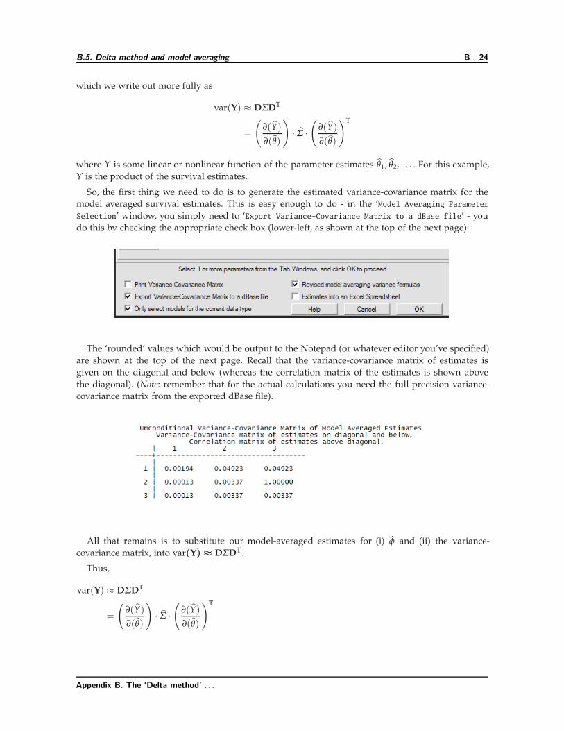
So, the first thing we need to do is to generate the estimated variance-covariance matrix for the

model averaged survival estimates. This is easy enough to do - in the ‘Model Averaging Parameter

Selection’ window, you simply need to ‘Export VarianceCovariance Matrix to a dBase file’ - you

do this by checking the appropriate check box (lower-left, as shown at the top of the next page):

The ‘rounded’ values which would be output to the Notepad (or whatever editor you’ve specified)

are shown at the top of the next page. Recall that the variance-covariance matrix of estimates is

given on the diagonal and below (whereas the correlation matrix of the estimates is shown above

the diagonal). (Note: remember that for the actual calculations you need the full precision variance-

covariance matrix from the exported dBase file).

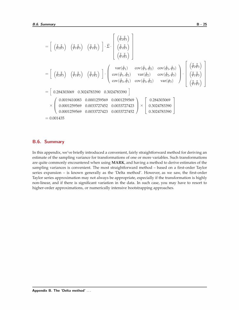
All that remains is to substitute our model-averaged estimates for (i) φ and (ii) the variance-

covariance matrix, into var(Y) ≈ DΣDT.

Thus,

var(Y) ≈ DΣDT

=

(∂(Y)

∂(θ)

)· Σ ·

(∂(Y)

∂(θ)

)T


B.6. Summary B - 25

=

[ (¯φ2

¯φ3

) (¯φ1

¯φ3

) (¯φ1

¯φ2

) ]· Σ ·

(¯φ2

¯φ3

)

(¯φ1

¯φ3

)

(¯φ1

¯φ2

)

=

[ (¯φ2

¯φ3

) (¯φ1

¯φ3

) (¯φ1

¯φ2

) ]·




·

(¯φ2

¯φ3

)

(¯φ1

¯φ3

)

(¯φ1

¯φ2

)

=[

0.284303069 0.3024783390 0.3024783390]

×

0.0019410083 0.0001259569 0.0001259569

0.0001259569 0.0033727452 0.0033727423

0.0001259569 0.0033727423 0.0033727452

×

0.284303069

0.3024783390

0.3024783390

= 0.001435

B.6. Summary

In this appendix, we’ve briefly introduced a convenient, fairly straightforward method for deriving an

estimate of the sampling variance for transformations of one or more variables. Such transformations

are quite commonly encountered when using MARK, and having a method to derive estimates of the

sampling variances is convenient. The most straightforward method – based on a first-order Taylor

series expansion – is known generally as the ‘Delta method’. However, as we saw, the first-order

Taylor series approximation may not always be appropriate, especially if the transformation is highly

non-linear, and if there is significant variation in the data. In such case, you may have to resort to

higher-order approximations, or numerically intensive bootstrapping approaches.


Documents

The ‘Delta method’ - Montefiore Institutekvansteen/MATH0008-2/ac20122013/Class2Oct... · Appendix B The ‘Delta method’ ... Suppose you have done a study, over 4 years, which