CHAPTER VI

THE ADAMS SPECTRAL SEQUENCE of H RING SPECTRA

by Robert R° Bruner

In this chapter we show how to use an H ring structure on a spectrum Y to pro-

duce formulas for differentials in the Adams spectral sequence of ~,Y. We shall

confine attention to the Adams spectral sequence based on mod p homology, although

it is clear that similar results will hold in generalized Adams spectra] sequences

as well.

The differentials have two parts. The first is the reflection in the Adams

spectral sequence of relations in homotopy like those in Chapter V. For example,

when x c ~n Y and n ~ 1 (4), there is no homotopy operation pn+lx since the n+l cell

of P~ is attached to the n cell by a degree 2 map. In the Adams spectral sequence n

there is a Steenrod operation Sq n+l x and a differential d2sqn+l x = hoSqn

= hoX~. Therefore hj 2 = 0 in E ~ This in itself only implies that 2x 2 has

filtration greater than that of h(~ in the Adams spectral sequence, but by

examining its origin as a homotopy operation we see that 2x 2 = O. Thus, the

formulas we produce for differentials are most effective when combined with the

results about homotopy operations in Chapter V. The differential d2sqn+3~=

hOSqn+21~ , still assuming n ~ 1 (4), is a perfect illustration of this. The

corresponding relation in homotopy is 2pn+2x = hlPU+lx where hl Pn+l is an indecom-

posable homotopy operation detected by hlSqn+l in the Adams spectral sequence. The

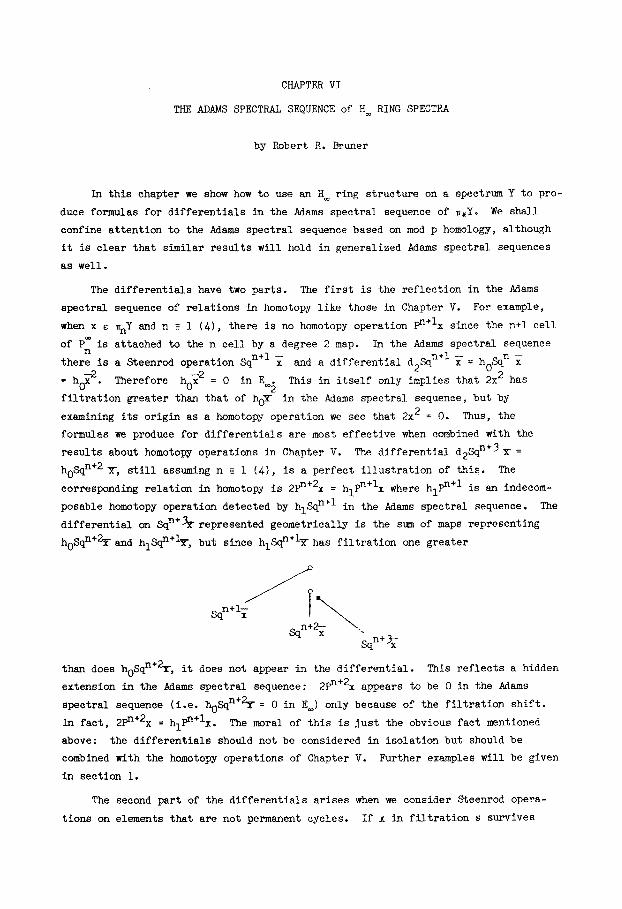
differential on sqn+Srrepresented geometrically is the st~ of maps representing

hOSqn+~xand hlSqn+l~- , but since hlSqn+l~has filtration one greater

jo

+ JJ

than does hOSqn+~ , it does not appear in the differential. This reflects a hidden

extension in the Adams spectral sequence: 2pn+2x appears to be 0 in the Adams

spectral sequence (i.e. hOSqn+2~ : 0 in E) only because of the filtration shift.

In fact, 2pn+2x = hlPn+Ix. The moral of this is Just the obvious fact mentioned

above: the differentials should not be considered in isolation but should be

combined with the homotopy operations of Chapter V. Further examples will be given

in section I.

The second part of the differentials arises when we consider Steenrod opera-

tions on elements that are not permanent cycles. If x in filtration s survives

170

until E r we can make x into a permanent cycle by truncating the spectral sequence at

filtration s+r. Thus the differentials of the type just discussed apply to x until

we get to F T • However, by analyzing the contribution of drX we can show that it

will not affect the differentials on 8~x until Epr_p+l where it contributes

8~P]drX. Thus the differentials of the first type apply far beyond the range in

which we are justified in pretending that x is a permanent cycle. (To be precise we

should note that drX can occasionally affect differentials on ~x through a term

containing xP-ldrx in Er+ 1 . )

The first results of this type were established by D. S. Kahn [47] who showed

that the H ring map ~2:W ~Z2 S (2) * S (obtained through coreductions of stunted

projective spaces) could be filtered to obtain maps representing the results of

Steenrod operations in ExtA(Zy,Zy) and that some differentials were implied by this.

Milgram [81] extended Kahn's work to the odd primary case and introduced the

spectral sequence of IV.6 which is by far the most effective tool for computing the

first part of the differential. His work was confined to the range in which it is

possible to act as if one is operating on a permanent cycle. Nonetheless he was

able to use the resulting formulas for differentials to substantially shorten

Mahowald and Tangora's calculation [61] of the first 47 stems at the prime 2 and to

catch a mistake in their calculation. The next step was taken by Makinen [62], who

showed how to incorporate the contribution of drX in the differentials on SqJx for

p = 2. Unfortunately, he apparently did not apply his formulas to the known calcu-

lations of the stable stems, for one of his most interesting formulas (published in

1973),

d~qJx = hlSqJ-Yx + SqJdyx if n - 1 (4),

combined with Milgram's calculation of Steenrod operations [81], implies that d3e I =

hlt , contradicting Theorem 8.6.6 of Mahowald and Tangora [61]. This application was

left for the author to discover in 1983. Note that the differential is out of

Milgram's range since a nonzero dyx prevents us from calculating d~x unless we

incorporate terms involving dyx. The argument in [61] that e I is a permanent cycle

is an intricate one, involving the existence of various Toda brackets, while the

that d3SqJx = hlSqJ-Yx + SqJdyx if n ~ 1 (4) is proof relatively straightforward.

This appears to be convincing evidence that the H= structure in the form of Steenrod

operations in Ext is a powerful computational tool.

One other piece of related work is the thesis of Clifford Cooley [30]. He

obtains formulas similar to Milgram's [61] by using the spectral sequence connecting

homomorphism for a cofiber sequence of stunted projective spaces to reduce them to

dl'S which he gets from a lambda algebra resolution of the cohomology of the

appropriate stunted projective space. Calculating differentials this way or by the

spectral sequence of IV.6 is probably a matter of indifference. The most

171

interesting aspect of Cooley's thesis is that he works unstably, examining the

interaction of the Steenrod operations and the EHP sequence. As in all other

earlier work on this subject he views the H ring structure in terms of coreductions

of stunted projective spaces. The interaction of the Steenrod operations and the

EHP sequence had been discovered by William Singer [97} using the algebraic F~P

sequence obtained from the lambda algebra.

In the work at hand, we extend the ideas of Makinen to the odd primary case to

obtain comprehensive formulas for the first nontrivial differential on ~Epjx, which

we state in §I. These apply to the mod p Adams spectral sequence of any H ring

spectrum. The remainder of §I consists of calculations using these formulas in the

Adams spectral sequence of a sphere, including the differential discussed above.

These are intended to illustrate especially the interaction between the homotopy

operations and the differentials, specifically to obtain better formulas in partic-

2 to be 2 which forces h 4 ular cases than hold in general. One of these is d3r = hld0,

a permanent cycle. This is the shortest proof we know of this fact.

In §§2 and 3 we describe the natural Zp equivariant cell decomposition of

(ZX) (p) and use it to relate extended powers of X and of zX.

in §4 we start the proof of the formulas in §i, using the results of ~§2 and 3.

We also prove that the geometry splits naturally into three cases, which we deal

with one at a time in the remaining §§5-7.

i. Differentials in the Adams spectral sequence

In this section we state our theorems concerning differentials, explain some of

the subtleties involved in understanding what they are really saying, and calculate

some examples in order to illustrate their use and demonstrate their power.

Localize everything at p. Let Y be an H ring spectrum. Let Es'n+S(s,Y) r

~n Y be the Adams spectral sequence based on ordinary mod p homology. We shall adopt

the following shorthand notation for differentials. If A is in filtration s and B 1

and B 2 are in filtrations s+r I and s+r 2 respectively, then

d,A = B 1 ~ B 2

means that diA = 0 for i < min(rl,r 2) and

drlA = B 1 if r I < r 2

drA = B 1 + B 2 if r I = r = r2, and

dr2A = ~ if r I > r 2

172 Note. This does not mean that this differential is necessarily nonzero. Nor does

it mean that if ~ happens to be 0, then dr2A = ~ regardless of whether r 2 > r I or

not. More likely, B 1 is zero because it comes from a map which lifts to filtration

s+rl+l or more and, hence, B 1 could conceivably lead to a nonzero drl+lA. The point

is that you can't tell what B 1 is contributing to the differential if all you know

is that it is zero in filtration s+r I . However, when we explicitly state that

Tp = 0 in Theorem 1.2 we mean that it is to be treated as having filtration ~.

The geometry behind the formula d,A = ~ ~ B 2 will make it clear exactly what

the formula can and cannot tell you. The formula means that for some r 0 > max(rl,r2) ,

A is represented by a map whose boundary splits into a sum B I + B2 + B0' where each

Bi lifts to filtration s+ri, and where B-- 1 and B2 represent B 1 and B 2 respectively.

It is irrelevant what B-- 0 represents because Bl+ B2 lies in a lower filtration.

This is fortunate, since in general B 0 is very complicated. In particular cases

however, we can often analyze B 0 in order to get more complete information about

d,A. For examples of this, see Proposition 1.17(ii) (the formula d3r 0 = hld ~) and

Proposition 1.6.

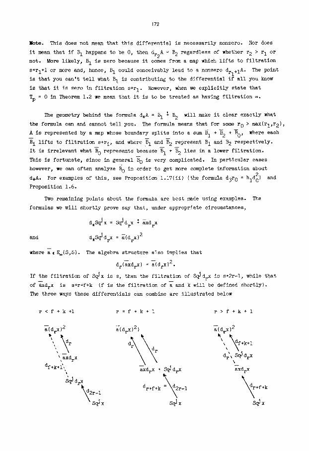
Two remaining points about the formula are best made using examples. The

formulas we will shortly prove say that, under appropriate circumstances,

and

where a E E~(S,S).

d, Jx = JdrX :

d,SqJdrx = ~(drXl 2

The algebra structure also implies that

dr(~XdrX) =~(drX) 2 .

If the filtration of S~x is s, then the filtration of SqJdrx is s+2r-l, while that

of~xdrx is s÷r+f+k (f is the filtration of~and k will be defined shortly}.

The three ways these differentials can combine are illustrated below

r < f ÷k+l r = f +k+l r > f +k+l

~(drX)2

\axdrx

d ~ f+k+l~

Sq J d rx

2r-I

s~x

~(drX)2) ~(drX) 2

\ \ +k+l \

d r ~ SqJ drX \

axdrx + @ drX aXdrX

dr+f+k -~2r-1 %~r+f+k s4,

173

Taken individually, the terms SqJdrx and~xdrx do not always appear to survive long

enough for S~x to be able to hit them. For example, when r > f+k+l, the

differential dr+f+kS~X =~XdrX is preceded by the differential dr(a--xdrx) =~(drX) 2,

which would have prevented axdrx from surviving until Er+k+f, had it not happened

that a still earlier differential (df+k+lS~drX : ~(drX)2) had already hit ~(drX)2.

This is completely typical. The formula d,A = B 1 + B2, as used here, carries with

it the claim that the right-hand side will survive long enough for this differential

to occur, and even shows the "coconspirator" which will make this possible when it

seems superficially false.

The other point illustrated by this example occurs when SqJdrx and XdrX are

permanent cycles and r > f+k+l. Then the differential dr+k+fSqJx = axdrx reflects

a hidden extension: ~(XdrX) is zero in E~ because of a filtration shift. It is

actually detected by SqJdrx. Relations among homotopy operations typically cause

such phenomena. Note that the cell which carries S@x is also the cell which pro-

duces the relation in homotopy. In a suitably relative sense this is the meaning

of all differentials in the Adams spectral sequence ("relative" because the terms

in a relation corresponding to a differential will typically be relative homotopy

classes which do not survive to E to become absolute homotopy classes).

We can now state our main theorems. Assume given x ~ E s'n+s and consider the r

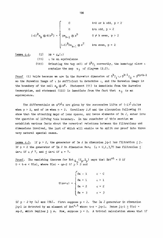
element 8S~x (as usual, c = 0 and ~ =SqJ if p = 2}. Let

k = ~j-n p = 2

[ (2j-n)(p-ll-a p > 2 ,

so that 8a~x ~ E~ s-k'p(n+s), which lies in the k÷np stem. Using the functions Vp

and ap of V.2.15, V.2.16 and V.2.17 we define v = Vp(k+n(p-1)) and

a = ap(k+n(p-1)) ~ ~v_l S. Recall that a is the top component of an attaching map

of a stunted lens space after the attaching map has been compressed into the lowest

possible skeleton. Let

EE~'f+v-I(s,s}

detect a (this defines f as well). Recall that a 0 ~E~ 'I~ detects the map of

degree p when p > 2.

Theorem I.i.

(i)

(ii)

There exists an element T ~E 2 (S,Y) such that

if p = 2 then d,SqJx = SqJdPx ~ T2,

if p > 2 then

dr+l~X = dr+lXP = a0xP-ldrx if 2j = n ,

d2~x = a0~x if 2J > n, and

d,G~x = -B~ drX ~ Tp

174

Theorem 1.2.

If p > 2 then

T 2

T P

I xx aSqJ-v x

v > k+l or 2r-2 < v < k

v = k+l

v = k or (v < k and v < I0)

0

(-l) e axP-ld x r

(_i) e-I ~B~ -e-I

v > k+l or pr-p < v < k

v = k+l

v < k and v < pq.

where e is the exponent of p in the prime factorization of J.

Note. When p > 2, k and v have opposite parity so that v = k never occurs.

Theorems I.I and 1.2 give complete information on the first possible nonzero

differential except when

pq < v < min(k,pr-p+l) if p > 2,

or i0 < v < min(k,2r-l) if p = 2.

The sketch of the proof given in Section 4 should mke it clear what the obstruction

is in these cases. We do have some partial information which we collect in the

following theorem.

Theorem 1.3. If p > 2 and v > q then di~PJx = 0 if i < v+2 < pr-p+l, while

d~r_p+l~PJx = -8~drX-- if v + 2 > pr-p+l. If p = 2 and v > 8 then diSqJx -- 0

if i < v+2 < 2r-l, while d2r_iSqJx = SqJdrx if v+2 > 2r-l.

To apply these results we must know the values of the Steenrod operations in

E 2 = Ext~(Zp,H,Y). For our examples we will concentrate primarily on p = 2 and

Y = S O , since this is a case in which there are many nontrivial examples. We cannot

resist also showing how useful the Steenrod operations are in the purely algebraic

task of determining the products in Ext.

~l ~2n-1 dual to the Sq 2n. Parts (i) and (iii) We begin with the elements h n E ~2

of the following propositon may also be found in [88].

Proposition 1.4. (i) (Adams [3]) sq2nhn = hn+ 1 and sq2n-lhn = ~.

:ii :Ad o, h 3 = hn%n÷: and h/n÷2 = O. n+l

2 n 9 9hinh - = 0 and, if n > O, h 0 h n = O. (iii) (Novikov [91] ) h2h2n n+3 = O, 0 n+2

175

Proof sq2n-lhn = h 2 because the first operation is always the square. If we let

S : Ext s , * Sq n+s ÷ Ext s,* be on Ext s,n+s, then Proposition ii.I0 of [68] shows that in

the cobar construction S[Xll... Ixj] = Ix21 I.-. Ix~]. Since h n is represented by

[~12n], it follows that sq2nhn = S(hn) = bn+ 1 . For dimensional reasons, the Caftan

formula reduces to S(xy) = S(x)S(y). Thus, to show (ii) we need only show hoh I = O,

= hoh2, and = O. These occur in such low dimensions that they may be

checked "by hand". In fact, only the first and third must be done this way since

+ h2h 2 Sq2(hoh l) = h2h2 hl3. The relation n n+3 = 0 follows similarly from

2 n+3 2 = h 2 hob32 2 = sqS(h 0 ) = O. The only nonzero operation on h 2n+2 is Sq h~+ 2 n+3

since (ii) implies that h 4 = hn+2(~+lhn+ 3) = O. The relation h2nh 2 = 0 then n+2 0 n+2

2 2 2 n follows by induction from hoh 3 = O. Finally, h 0 h n = 0 follows by induction from

h2h I = 0 since

2 n 2 n 2 n+l Sq (h 0 hnl = h 0 hn+ I .

As is well known, the preceding proposition implies the Hopf invariant one

differentials.

Corollary 1.5. d2hn+ 1 : ~ for all n > O.

Proof. By Theorems I.i and 1.2 we find that

= ~ 2 n • 2 d,hn+ 1 d,sq2n~ = Sq d2h ~ ÷ hob n

2 so that d2hn+ I = hoh n

2 n since Sq d2h n is in filtration 4. (It follows, of course, that

2 n 2n h 2 Sq d2h n = Sq Onn_l = h~.)

The next result shows how we may use the relation with homotopy operations to

get stronger results than the differentials themselves give.

Proposition 1.6. hlh 4 and ~h 4 are permanent cycles.

Proof. Since hlh 4 = Sq9(hoh3) , it is carried by the 9-cell of P~. The attaching

map is ~, to the 7-cell, and hence its boundary is u(2~) 2 = O. Similarly, h2h 4 =

sqlO(hlh3) , so h2h 4 is carried by the lO-cell of p~O = $8v($9 2 elO). The 9-cell

carries p9(o~), which has order 2 by the Caftan formula in Theorem V.l.lO. Thus,

the boundary of the lO-cell maps to 0 and h2h 4 is a permanent cycle.

176

Before turning to other families of elements we should note that the Hopf

invariant one differentials of Corollary 1.5 account for only a few of the non-

trivial differentials on the h~hn+ 1. In fact, Proposition 1.4 implies

i d2hoh+ li = hi+lh20 n is 0 if i+l _> 2 n-2. On the other hand, hoh+l / O for

i < 2 n+l, and from the known order of Im J, there must be higher differentials on

of the h~h+lv~, which survive to E 3. It seems difficult to determine these many

higher differentials in terms of the Steenrod operations, though Milgram [811 has

indicated that it may be possible with a sufficiently good hold on the chain level

operations. More disappointing is the fact that it doesn't seem possible to pro-

pagate these higher differentials. That is, even if we accept as given a differ-

d3hoh 4 = hodo, we don't seem to get any information on d3h~h 5. ential like

The operation we call S in Proposition 1.4 will be very useful so we collect

its properties before proceeding.

Prgposition 1.7. If S = sqn+S:Ext s,n+s * Ext s'2(n+s) then

S[Xll...Ix k] = [x~l...Ix ~] in the cobar construction (i)

(ii) S(xy) = S(x)S(y)

(iii) SqJsx = SSqj-n-Sx

(iv) S<xo,Xl,...,Xn > C <Sxo,SXl,...,SXn>

Proof. (i) is Proposition Ii.I0 of [68], while (ii) and (iii) are immediate from

the Cartan and Adem relations since all the other terms must be 0 for dimensional

reasons. Part (iv) is proved in [78].

For our remaining sample calculations we will explore the consequences of the

squaring operations on the elements Co, do, e 0 and fo" The key elements we will be

concerned with are collected in Table 1.1 along with Massey product representations.

With the exception of fo and YO, the Massey products have no indeterminacy.

177

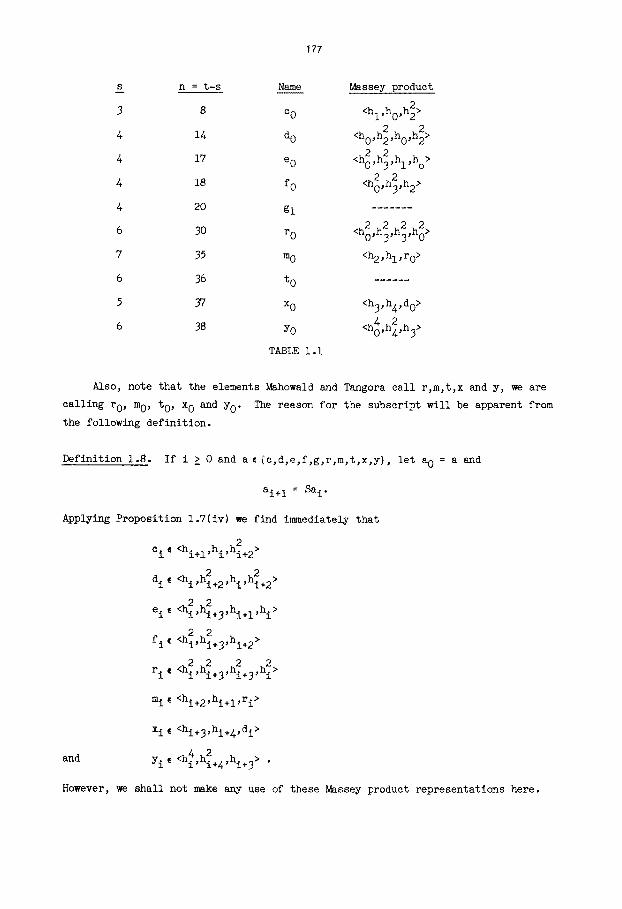
s n = t-s Name Massey product

3 8 C O <h I,hO,h22>

2 2 4 14 d O <h0,h 2,hO,h2 >

2 2 > 4 17 e 0 <h 0,h 3,h I ,h O

2 2 4 18 fo <ho'h3'h2>

4 20 gl .......

2 2 2 2 6 30 r 0 <h0,h3,h3,h0>

7 35 m 0 <h 2 ,h I , ro>

6 36 t o ......

5 37 X 0 <h3,h4,d0>

<h 4 2 . 6 38 Y0 0,h4,n3 >

TABLE i.I

Also, note that the elements Ri~howald and Tangora call r,m,t,x and y, we are

calling to, mo, to, x 0 and YO" The reason for the subscript will be apparent from

the following definition.

~finition 1.8. If i £ 0 and aE {c,d,e,f,g,r,m,t,x,y}, let a 0 = a and

ai+ 1 = Sa i.

ApplylngProposition 1.7(iv) we find in~medlate~ that

2 c i E <hi+l,hi,hi+2 >

2 2 d i ¢ <hi,hi+2,hl,hi+2 >

22 e i E <hi,hi+3,hi+l,hi>

< 2 2 > fi E hi,hi+3,hi+2

22 2 2 r i E ~i,hi+3,hi+3,hi>

miE <hi+2,hi+l,ri >

x i t <hi+3,hi+4,di>

<~4.2 and Yi E ni,ni+4,hi+3> .

However, ~ shall not make any use of these ~ssey product representations ~re.

178

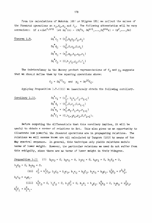
From the calculations of Mukohda [88] or Milgram [81] we collect the values of

the Steenrod operations on co,do,e 0 and fo" The following abbreviation will be very

convenient: if x EExt s,n+s let Sq*(x) = (Sqnx, sqn+l,...,sqn+Sx) = (x2,...,Sx)

Theorem 1.9. * 2 Sq c o = (Co,hoeo,fo,C I)

* 2 Sq d O = (do,O,ro,O,dl)

* 2 Sq e 0 = (eo ,mo, to ,Xo,e 1)

Sq f0 = (0'h3r0'Y0'0'fl)

The indeterminacy in the Massey product representations of fo and YO suggests

that we should define them by the squaring operations above:

fo : Sql0co and YO = sq2Ofo"

Applying Proposition 1.7.(iii) we immediately obtain the following corollary.

Corollary i.i0. , 2 Sq c i = (ci, hiei,fi,ci+ I)

Sq*d i = (d~,0,ri,0,di+ l)

Sq*e i = ( e ~ , m i , t i , x i , e i + 1)

Sq fi = (0,hi+3ri,Yi,0,fi+l)"

Before computing the differentials that this corollary implies, it will be

useful to obtain a number of relations in Ext. This also gives us an opportunity to

illustrate how powerful the Steenrod operations are in propagating relations. The

relations we will assume known are all calculated by Tangora [IO3] by means of the

May spectral sequence. In general, this technique only yields relations modulo

terms of lower weight. However, the particular relations we need do not suffer from

this ambiguity, since there are no terms of lower weight in their bidegree.

Proposition i.ii

hlr 0 = O, hlm 0 = O.

(ii)

h2t 0 = clg I.

(iii)

h2fl = <e I •

(i) hoc 0 = O, h2c 0 = O, h3c 0 = O, hoc I = O, hlf 0 = O,

2 2 = = C O = hldo, h2do = hoe O, hle 0 hof O, h2e 0 = hogl, h~d 0 plh2,

= = 2 = h6x 0 0, = 2 h6r 0 O, h4f 0 0, h3d 0 = 0, h2d I h4gl, = h2m 0 h0Y0,

179

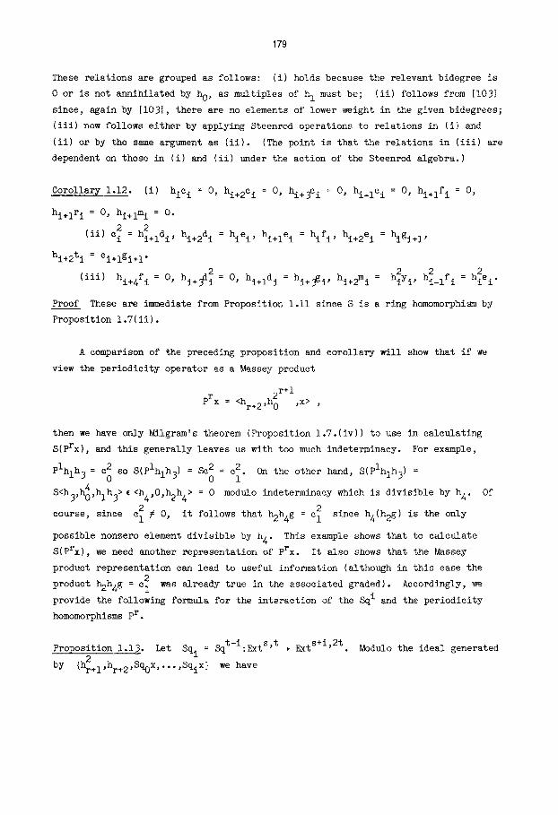
These relations are grouped as follows: (i) holds because the relevant bidegree is

O or is not annihilated by ho, as multiples of h I must be; (ii) follows from [103]

since, again by [103], there are no elements of lower weight in the given bidegrees;

(iii) now follows either by applying Steenrod operations to relations in (i) and

(it) or by the same argument as (it). (The point is that the relations in (iii) are

dependent on those in (i) and (it) under the action of the Steenrod algebra.)

Corollar~ 1.12. (i) hic i = O, hi+2c i = O, hi+3c i = O, hi_ic i = 0, hi+if i = 0,

hi+lr i = O, hi+im i = O.

(it) c 2 2 i = hi+ldi' hi+2di = hiei' hi+let = hifi' hi+2ei = higi+l'

hi+2t i = Ci+lgi+ 1.

= 2 h~_If i h~ei. (iii) hi+4f i O, hi+~ = O, hi+id i = hi+~i , hi+2mi = hiYi, =

Proof These are immediate from Proposition I.Ii since S is a ring homomorphiam by

Proposition 1.7(ii).

A comparison of the preceding proposition and corollary will show that if we

view the periodicity operator as a Massey product

_r+l pr x <hr+2'h~ u ,x> ,

then we have only Milgram's theorem (Proposition 1.7.(iv)) to use in calculating

s(prx), and this generally leaves us with too much indeterminacy. For example,

plhlh 3 = c 2 so s(plhlh 3) = Sc 2 = c 2. On the other hand, s(plhlh 3) = 0 0 I

S<h3,h~,hlh3>__ E <h4,0,h2h4> = 0 modulo indeterminacy which is divisible by h 4. Of

course, since c~ / O, it follows that h2h4g = c~ since h%(h2g) is the only

possible nonzero element divisible by h 4. This example shows that to calculate

s(prx), we need another representation of prx. It also shows that the Massey

product representation can lead to useful information (although in this case the 2

product h2h4g = c I was already true in the associated graded). Accordingly, we

provide the following formula for the interaction of the Sq i and the periodicity

homomorphisms pr.

= Sq t-i + Ext s+i'2t. Proposition 1.13. Let Sqi :Ext s't Modulo the ideal generated

by {h~+l,hr+2,Sq0x,...,Sqix } we have

180

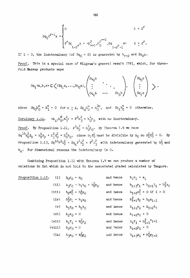
SqiPr-lx = I O ~r+l i < 2 r

prsql._2rX + <h~+l,h ~ ,Sqi_2r_iX> i _> 2 r .

If i = O, the indeterminacy (of Sq 0 = S) is generated by hr+ 2 and Sqox.

Proof. This is a special case of Milgram's general result [78], which, for three-

fold Massey products says

S% <a,b,c> C ((S%a,...,S%a), V'h b "%b \sq ic/

n - o for n > ' . % h o = hon. and qiho = 0 otherwise . SinCe S q o h 0 = h I

8 2 = p~ : h04r 0 with no indeterminacy. Corollary 1.14. <h4,ho,h 3>

Proof. By Proposition i.II, P = hod O. By Theorem 1.9 we have

S162 04 22 04 22 q h0do = h r 0 + hld 0 = h ro, since hl d2 must be divisible by h O so hld 0 = O. By

Proposition 1.13, Sql6plh2 = Sq4Pl~ = i:'24 with indeterminacy generated by h~ and

h 4. For dimensional reasons the indeterminacy is O.

Combining Proposition l.ll with Theorem 1.9 we can produce a number of

relations in Ext which do not hold in the associated graded calculated by Tangora.

Proposition 1.15. (i) h0r 0 = s o and hence hir i = s i

(ii) h3r 0 = hlt 0 + h~o and hence hi+3r i = h-+~t.1 ± I + h~xi

(iii) h2e ~ = h~x 0 and hence hi+2e [ = 0 if i > 0

(iv) h~d I = hlX O and hence h~+id i = hixi_ 1

(v) hlY O = h2t 0 and hence hi+lY i = hi+2t i

(vi) h2x 0 = O and hence hi+2x i = 0

(vii) hlf I = h~c 2 and hence hif i = h[_lCi+l

(viii) h2Y 0 = 0 and hence hi+2Y i = 0

(ix) h3x 0 = h~2 and hence hi+~x i " h~gi+ 2

181

Note. Mahowald and Tangora [61] found (i)-(iii) by other techniques. Barratt,

Mahowald and Tangora [20] also found (iv), (vii), and (ix) by other techniques.

Milgram [81] found (i) and (ii) by using the Steenrod operations. Mukohda [88]

found (iv)-(vi) and (ix), partly by using the Steenrod operations and the cobar

construction, and partly by means of a minimal resolution.

Proof. Given (ii), (i) follows because hoh3r 0 = h~x 0 ~ O, from which it follows

that hot 0 ~ O. The only possibility is hor 0 = s O . To prove (ii), apply Sq 20 to the

relation h2d 0 = hoe O. To prove (iii), apply Sq 19 to the relation

hle 0 = hof 0 and use the fact that hlm 0 = O. To prove (iv), apply Sq 21 to the

relation h2d 0 = hoe 0 and use the fact that h~e I = O. To prove (v), apply Sq 21 to

the relation hle 0 = hof 0 and use (iv) to show that h~x 0 = hl(h~d l) = O. To prove

(vi), apply Sq 22 to the relation hle 0 = hof 0 to show that h2x 0 = h~e I + h~fl, and

apply Proposition 1.11.(iii) to show that this is O. For (vii), we apply Sq 22 to

hoe I = O. Similarly, Sq 21 applied to hlf 0 = 0 yields (viii). Finally, (ix) follows

by applying Sq 24 to the relation h2e 0 = hog I to get h~2 = h3x 0 + h~el, and noting

that h~e I = h2(hlf I) = O. The calcultion of Sq24(hogl ) is possible because Sq24g I =

g2 by definition, while Sq23g I = 0 for dimensional reasons.

Now we examine the differentials implied by the squaring operations in the ci,

di, e i and fi families. The results we obtain for t-s > 45 are all new. In the

range t-s ~_ 45 they are due to May [66], Maunder [65], Mahowald and Tangora [61],

Milgram [81] and Barratt, Mahowald and Tangora [20] with the exception of d3e I =

hlt , which is new and corrects a mistake in [20]. As noted by Milgram [81] the

proofs using Steenrod operations are usually far simpler and more direct than the

original proofs. In addition, when they replace proofs which relied on prior

knowledge of the relevant homotopy groups we obtain independent verification of the

calculation of those homotopy groups.

Es,n+s If x ~ r , let us write x c (s,n) or x ~ (s,n) r for convenience. Theorems

1.1, 1.2 and 1.3 imply that

d*SqJx = SqJdrx $ I ~XdrxO vV => k+Ik+l or 2r-2 < v < k

L aSqj-Vx v = k or (v < k and v < lO)

where k = j-n, v = 8a + 2 b if j+l = 24a+b(odd), and a detects a generator of Im J

in ~v_l SO •

We start with a general observation about families {ai} with ai+ I = S(ai). If

a i ~(s,n i) then

n i + s = 2(hi_ 1 + s) = 2i(no + s).

182

If N is the integer such that 2 N-I < s+2 < 2 N then the differentials on the elements

SqJa i depend on the congruence class of n i modulo 2 N. Clearly, n i ~ -s modulo 2 N if

i ~ N. Thus, the differentials on all but the first N members of such a family

follow a pattern which depends only on the filtration in which the family lives.

Consider the c i family. We have c O E (3,8)~, so in general c i ~ (3,2i.II-3).

Proposition 1.16. (i) c I ~E while d2c i = hofi_ 1 for i ~ 2

(ii) d2f O = h~eo, fl ~ES' and d3f i = hlYi_ 1 for i ~ 2

(iii) d3c ~ = h~i+2ri_ 1 for i ~ 2

Note. We will show shortly that d2h0Yi_ 1 = h~i+2ri_ I. This, together with (iii)

implies that d3c ~ = O.

Corollary 1.17. d2e O = c 2 and v84 ~ O, where 84 is the Arf invariant one element

detected by h~.

Proof. Since e 0 ~ (3,8)~, Sq*c 0 = (c2,h0eo,f0,cl) is carried by

z8p~l= SI6v (sl?kj 2 el8)v S 19. Therefore c I ~ E= and d2f 0 = h2e O. Applying

Proposition I.ii we find that d2hle 0 = d2hof O = h~e 0 = h~d 0 = hlC2 , from which it

follows that d2e O = c 2.

Since c I E (3,19)=, Sq*c I (c2,hlel,fl,c2) is carried by _19~23 = ~ :19 =

(S 38 k_/2 e 39 e 40 ) e 41 = U/n k.; 2 • Therefore d2c 2 = h0f I and d3f I = hlC2 = hlh22dl O,

so that fl ~ E 5 for dimensional reasons. Since c 2 = <h3,h2,h~> and c 2 ~E., the Toda

bracket <c,v,04> does not exist. We shall show in the next proposition that h~E E

so that e 4 exists. Since Gv = O, it follows that v84 ~ 0.

Now assume for induction that d2ci = hofi_12 and that i > 2. We can arrange the

relevant information in the following table.

j (mod 41 SqJc i SqJ(h0f2_l) k v a

1 e 2 h2h.+~r, i 0 2 h I U 1 E I--

2 l 1 h o 2 hie i hoYi_ I + hlhi+2ri_ I

3 fi hlYi-i 2 > 4 -

4 ci+ 1 h02fi 3 1 h 0

183

It follows that d3c~ = 2 hohi+2ri_l, d2hie i = hock, d3f i = hlYi_ I and d2ci+ 1 =

hof i. This completes the inductive step and finishes the proof of Propositon 1.16

and Corollary 1.1% Note that we have omitted d2hie i from the statement of the

proposition because it will follow from our calculation of d2e i below.

Proposition 1.18. (i) d2k = hod ~

2 (ii) d3r 0 = hld 0 and h~ ~E

(iii) r i ~E 3 for i Z 1

(iv) di~ E 3 for i ~ I

Note. Mahowald and Tangora show 161] that d I is actually in E , not just E 3. Also,

the proof given here that h~ ~ E is much simpler than the proof in [61].

Proof. Since d O c (4,14)~, Sq*d 0 (d~, O, ro, O, d I) is carried by 14~18 which = z ~14'

has attaching maps as shown

18 ~ d I

17

16 r 0

15 2

14 d O

Now d3hoh 4 = hod 0 implies h0d2 = 0 in E 4. The only possibility is that d2k :

hod2. This implies that 2~29 = O. Since the boundary of the 16 cell carries hl d2

plus twice something, we get d3r 0 = hld20 . Nothing is left for h 2 to hit, so h 2 c E=. 4 4

Finally, d2(d l) = h0.0 = 0 so d lc E 3. Now assume for induction that i > 1 and

d i ~ E 3. The terms SqJd3d i in the differentials on SqJd i will not contribute until * 2 E5, so will not affect the proof of (iii) and (iv). Since Sq d i = (di,O,ri,O,di+ l)

we find that d2r i = ho.O = 0 and d2(di+ l) = ho.O = O, proving (iii) and (iv) and

completing the induction.

Proposition 1.19. (i) d2m O = hoe2 , t o ~EII and d3e I = hlt O

(ii) el 2 E E5, d5m I = Sq39hlto, d2t I = homl, d3x I = hlm I and d2e 2 = hox 1.

2 sqnhOX i-I ' (iii) If i > 2 and n = 2i.21 - 4 then d3e2 = hoeiXi_ 1 +

d3m i = sqn+lhoxi_l , d2t i = h0mi, d3x i = sqn+3hoXi_l , and d2e i = hoxi_ 1.

Proof. By Corollary 1.17, d2e 0 = c 2. The information needed to calculate the

differentials on the SqJe 0 is most conveniently presented in a table.

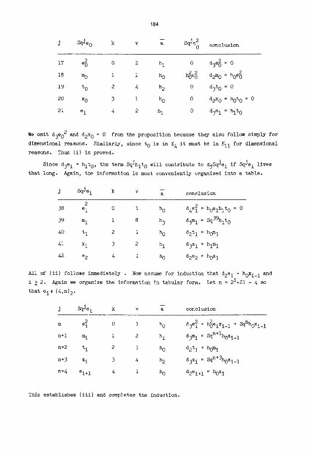
184

J SqJe 0 k v a SqJc~ conclusion

17 e 2 0 2 h I 0 d3e2-- 0

18 m 0 i I h 0 ~e 2 d2mo = ho e2

19 t o 2 4 h 2 0 d3t 0 = 0

20 x 0 3 1 h 0 O d2x 0 = hot 0 = 0

21 e I 4 2 h I 0 d3e I = hlt 0

We omit d3eo 2 and d2x 0 = 0 from the proposition because they also follow simply for

dimensional reasons. Similarly, since t O is in E 4 it must be in Ell for dimensional

reasons. Thus (i) is proved.

Since d3e I = hlt0, the term SqJhlt 0 will contribute to dsSqJe I if SqJe I lives

that long. Again, the information is most conveniently organized into a table.

SqJ j e i k v a conclusion

2 d4e~ = 38 e I 0 1 h 0

39 m I 1 8 h 3 dsm I =

40 t I 2 i h 0 d2t I =

41 x I 3 2 h I d3x I =

42 e 2 4 i h 0 d2e 2 =

All of (ii) follows immediately . Now assume for induction

i £ 2. Again we organize the information in tabular form.

that e iE (4,n) 2.

j SqJe i k v ~ conclusion

hoelhlt 0 = 0

Sq39hlt 0

hom 1

hlm 1

hox I

that d2e i = hoxi_ 1 and

Let n = 2i.21 - 4 so

n e~ 0 1 h 0

n+l m i 1 2 h 1

n+2 t i 2 I h 0

n+3 x i 3 4 h 2

n+4 ei+ 1 4 I h 0

This establishes (iii) and completes the induction.

d3e2 = h2eixi_l + sqnhOXi_ 1

d3m i = sqn+lhoxi_l

d2t i = horn i

d3x i = sqn+3hoXi_l

d2ei+ 1 = hox i

185

Note that three of the 5 entries in the above table satisfy v = k+l. The

corresponding differentials therefore contain terms of the form axdrx , specifically

ahOeixi_ 1 in this instance.

Only one of the differentials on the SqJf i is interesting.

Proposition 1.20. For all i ~ O, d2Y i = h0hi+3r i.

Proof. The terms in d.SqJx involving drX do not contribute to d2SqJx.

If n = 2i.22 - 4 so that fie (4,n) then sqn+If i = hi+3r i and sqn+2f i = Yi"

n+2 is even the proposition follows immediately.

Since

This completes our sampler. We have calculated only about one fourth of the

differentials found by Mahowald and Tangora, but they include some of the most

difficult. The remaining differentials follow more or less directly from those

calculated here just as in Mahowald and Tangora's original paper [61].

2. Extended Powers of Cells

In order to study Steenrod operations on elements of the Adams spectral

sequence which are not permanent cycles, we need a relative version of the extended

power construction. The extended power functor E~ ~ X (p), for ~ C Zp, factors as

the composite of the functors

X: ~X (p)

and Y~ ~E~ ~ Y

If we replace X by a pair (X,A) then X (p) is replaced by a length p+l filtration

X (p)) ... ) A (p) of ~ spectra and we may apply E~ ~ (?) to this termwise. The

resulting diagram is the relativization which we need. While the formalism applies

to any pair (X,A), we will confine attention to pairs (CX,X), where CX is the cone

on X, both for notational simplicity and because the pth power of such a pair has

special properties which we shall exploit. In particular, note that Lemma 2.4 is

the geometric analog of the fact that a trivial one-dimensional representation

splits off the permutation representation of ~ C Zp on R p. Most of this section is

devoted to this fact and its consequences.

An element x ~ Es'n+S(x,Y) can be represented by a map of pairs r

(CX,X) ~ (Ys,Ys+r).

Extended powers of (CX,X) can be used to construct a map representing ~PJx. The

186

final bit of the section establishes the facts about extended powers which will

enable us to construct and analyze such a map.

We shall work first in the category of based ~-spaces and based n-maps and the

homotopy category of based n-spaces and ~-homotopy classes of based ~-maps with weak

equivalences inverted. The results are then transferred to the category of n-spectra

by small smash products, desuspensions, and colimits.

Let I be the unit interval. We choose 0 as the basepoint, justifying our

choice by the resulting simplicity of the formulas in the proof of Lemma 2.4. For a

space or spectrum X, let CX = X ^I. The isomorphism X ~ X ̂ {0,I} and the

cofibration {0,I} C I induce a cofibration X + CX with cofiber ZX.

Definition 2.1. For a space X, define a Zp-space ri(X) by

E (CX) (p) I at least i of the c. lie in X}. ri(X) = {el^ ...^ Cp J

If X is a spectrum, define a Zp spectrum Fi(X) = X (p)^ ri(S0).

Lemma 2.2. (i) For a space X, ri(X) is naturally and Zp equivariantly homeomorphic

to x(P)^ ri(sO).

(ii) Fi(Z®X) ~ Z=FI(X) if X is a space.

(iii) ri+l(X) + Fi(X) is a Zp-COfibration.

(iv) ri(X)/Fi+l(X) is equivalent to the wedge of all (i,p-i) permutations

of X (i) ~ (ZX) (p-i). In particular, if (p) is the permutation

representation of Zp on R p then ro(X)/Fl(X) ~ (zX) (p) ~ z(P)x (p)

and rp(X) ~ X (p)"

(v) rl(X) ~ zP-Ix (p) as Zp spaces or spectra, where S p-I has the Zp action

inherited from the p-cell ro(S O) : I (p).

Proof. (i) follows immediately from the shuffle map

(xl^tl)^ .-. ̂ (Xp^tp) ~ (xl~-..^Xp) ^(tl^ ---Atp)-

(ii) is a consequence of the commutation of Z ~ and smash products.

(iii) follows for spectra if it holds for spaces. By (i) it holds for spaces

if it holds for S O . For S O , it follows because ri{S O) is the (p-i) skeleton of a CW

decomposition of ro(S O) = I (p).

Similarly, (iv) holds in general if it holds for S O , for which it is immediate.

(v) follows from the fact that rl(S O) is the boundary of the p-cell to(SO).

187

Remark 2.3: We will complete what we have begun in (iv) and (v) above in Lemma 3.5,

which shows that

Fi(X) = V znp-ix (p)- (p-i,i-l)

The next lemma is the key result of this section. Let I and S 1 have trivial Zp

actions so that if X is a Zp space or spectrum then CX = X^I and ZX = X^S 1 are

also.

Lemma 2.4. There are natural equivariant equivalences F0(X) ~ Crl(X) and

ZFI(X) ~ (ZX) (p) such that the triangle

0 Crl(X)

q(x) Ill con~nutes. ~ ~o(X)

Proof. By definition and by 2.2(i) we may assume X = S O . We define a Zp

homeomorphism ro(SO) + CFI(SO) by

t I t t I^ ...^tp .... ~ (%--^...^t -~)^t

where t = max{ti}. The inverse homeomorphism is given by

(tl^ ... At )^t ~ >tt l^tt 2^... ^tt P P

Commutativity of the triangle is immediate. The equivalence ZFI(X) ~ (ZX) (p)

follows since Zrl(X) ~ Crl(X)/rl(X) ~ F0(X)/FI(X) ~ (zX) (p), the latter equivalence

by 2.2(iv).

Lemma 2.5. For any ~ C Zp and any n-free ~ space W, there are natural equivalences

W K r0(X) ~ C(W~ rl(X))

and Z(W ~ rl(X)) ~ W~ (ZX) (p)

such that the following triangle commutes.

W ~ rl(X) ~,~,,~ wIi~ ~ r°(x)

" ~ C(W ~ rl(X))

Proof. By Lemma 2.4, W ~ to(X) ~ W ~(rl(X)^l) and by l.l.2.(ii)

W~ (FI(X)^I) = (w~ FI(X))^I = C(W~ FI(X)). The second equivalence follows

similarly. Commutativity of the triangle follows from naturality with respect to

{0,I} C I.

188

In the remainder of this section we shall restrict attention to the special

case of interest in section 4. The general case presents no additional difficulties

but is notationally more cumbersome.

Let w C Zp be cyclic of order p and let W = S ~ with the cell structure which

makes C,W ~ ~, the usual Z[~] resolution of Z. Let W k be the k-skeleton of W.

As in V.2, wk/~ is the lens space ~k, and, by 1.1.3.(ii), if r i = ri(S n-l) then

W k~ ri/wk-i ~ ~kr i" r i = By Lemmas 2.2 and 2.5 we then have the following

corollary of Theorems V.2.6 and V.2.14.

= zn-i ~(n-l)(p-l)+k Corollary 2.6: wk~ rp b(n-l)(p-l)

and wk× rl zn-i %n(p-l)+k ~n(p-l) "

Now note that Lemma 2.5 also implies that ~a F 1 k_)W k-I ~ r 0 is the

cofiber of the inclusion W k-I ~ r I ÷ W & ~ r I. By Corollary 2.6 or by Lemma 2.2

and 1.1.3.(ii) it follows that

Snp+k-l.

To get this equivalence in a maximally useful form, first consider a more general

situation. In order to analyze the Barratt-Puppe sequence of a map a:A + X one

constructs the diagram below.

(2.1)

A - ~ CA

. . . . CA = X~a CA

......... ~A i(i(a))

•Ci(a) = Xk~ a CAkJi(a) CX

In diagram (2.1) the front and back squares are pushouts, a 3 is an equivalence,

a 2 = Ca = a^l, a I is the obvious natural inclusion, and the maps a, i(a), and

a~li(i(a)) are the beginning of the cofiber sequence of a. The following obvious

fact about such diagrams will be used repeatedly.

Lemma 2.7. Let B + Y be a cofibration and let ~:Y + Y/B be the natural map. For

any map

f:(Ci(a),X) + (Y,B),

we have ~fa 3 = fa I - fa 2 in [zA,Y/B], where fa i is the map zA + Y/B induced by

(fai,fa):(CA,A) + (Y,B).

189

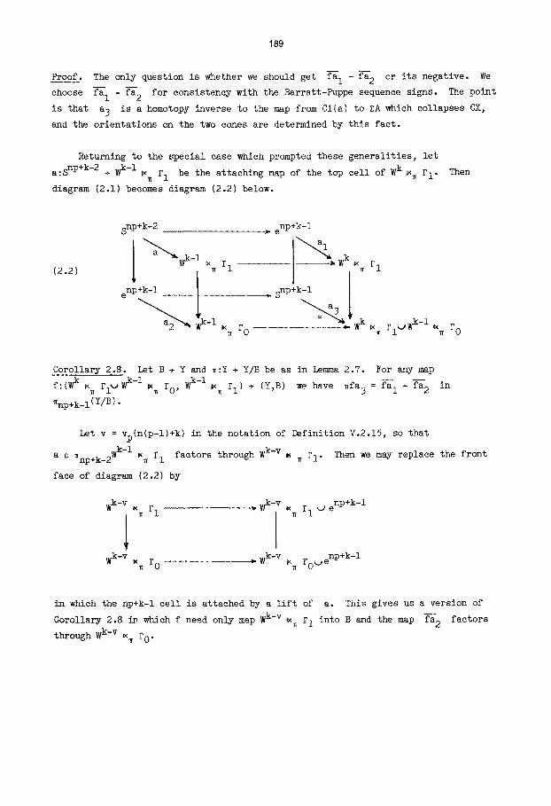
Proof. The only question is whether we should get fa I - fa 2 or its negative. We

choose fa I - fa 2 for consistency with the Barratt-Puppe sequence signs. The point

is that a 3 is a homotopy inverse to the map from Ci(a) to ZA which collapses CX,

and the orientations on the two cones are determined by this fact.

Returning to the special case which prompted these generalities, let

a:S np+k-2 +W k-1 ~ r I be the attaching map of the top cell of W k s~ r 1.

diagram (2.1) becomes diagram (2.2) below.

Then

(2.2)

Snp+k-2

enP +k-I __ [

~ w ~-I ~ r 0

enP +k-I

a 1

~ rl

S np+k-I 1

= ~ ~ w k ~ . rl~Wk-I ~ r o

Corollary 2.8. Let B + Y and ~:Y ÷ Y/B be as in Lemma 2.7. For any map

f:(W k ~ FI~.~W k-I ~ rO , W k-I ;x~ F I) + (Y,B) we have ~fa 3 = fa--- 1 - fa--- 2

~np÷k-1 (Y/B) .

in

Let v = Vp(n(p-l)+k) in the notation of Definition V.2.19, so that

a a ~np+k_2 Wk-1 ~ r I factors through W k-v ~ ~ r 1. Then we may replace the front

face of diagram (2.2) by

W k-v ~( F I ~ W k-v ,< F 1 <2 e np+k-1 7T

W k - v k r 0 W k-v ~ rou~e np+k-I

in which the np+k-I cell is attached by a lift of a. This gives us a version of

Corollary 2.8 in which f need only map W k-v ~ r I into B and the map fa 2 factors

through W k-v ~ r 0.

190

§3. Chain Level Calculations

In this section we define and study certain elements in the cellular chains of

W ~ rO(Sn-1). In sections 5-7 they will be used to investigate the homotopy groups

of various pairs of subspaces of W m F0(sn-1). Here we use them to determine the

effect in homology of a compression (lift) of the natural map W k m Fp(S n-l) +

W k ~ FI(Sn-I).

Let r i = Zi(sn-1). Give e n = C(S u-l) the cell structure with (me n-cell x and

one (n-1)-cell dx. Let C,(?) denote cellular chains and C,(?;R) = C,(?)OR. Then

C,Y 0 = <x,dx> p, the p-fold tensor product of copies of C,(e n) = <x,dx>, and

Cirj =I CiFO0 ii j> nP~np~

We shall find it convenient to omit the tensor product sign in writing elements of

C.Fj, so that, for example, xP-ldx denotes x Q x® ... ~)x~)dx. Let W = S ~ with

the usual ~-equivariant cell structure. Then C,W is the minimal resolution ~of Z

over Z[~]. Let

~Ir(k)J = I O~j j > k J ~ k

so that ~(k) = C,(wk), where W k is the k-skeleton of W. Then by I 2.1,

c,(w k % r i) ~ ~(~I ®~ c,~ Let G be the p-cycle (i 2 ... p) in ~ C Zp, and let ~ and Zp act on

C,F i by permuting factors. Following [68, Theorem 3.11 we define elements

t i ¢ C,F 0 as follows. Define a contracting homotopy for C,F 0 by s(ax) = 0

and s(adx) = (-l)lalax.

Definition 3.1. If p = 2, let t O = dx 2, t I

N = I + ~ + 2 + ... + ~p-l. Let

t O = dx p , t I = dxP-lx,

t2i = s((m -I - l)t2i_l) , and

t2i+l = s(Nt2i)°

= xdx, and t 2 = x 2. If p > 2, let

Lemma 3.2. (i) If p = 2 then d(t 2) : (a + (-l)n)tl and d(t I) = t O .

(ii) If p > 2 then d(t l) = to,

d(t2i) = (a -1 _ 1)t2i_l

and d(t2i+l) = Nt2i if i > O.

191

(iii) If p > 2 then tp = (-l)mnm!x p and

tp_ 1 = m!xP-ldx + (m-l)!(~ -I _ l)QxP-ldx

m

where m = (p-l)/2 and Q = (~+I) ~ i~ 2i i=l

Proof. (i) and (ii) are easy calculations, by induction on i for d(t2i) and

d(t2i+l) using (a-l-1)N = O = N(a-l-1) and ds + sd = 1.

In [68,Theorem 3.1] it is shown that tp = (-1)Hmm!x p and that

tp_ 1 = (m-1)!PxP-ldx, where p = ~ + 3 + ... aP-2. Since P = m + ( -I _ 1)Q,

(iii) follows.

Lemma 3.3. If p = 2, then in C,(W i+l ~ F I)

J (-1)iei ® d(x 2) n ~ i (2)

ei+ 1 ® dx 2 ~

(-1)ie i® d(x 2) - 2e i® xdx n ~ i (2)

Proof. We have d(e i) = (~ + (-1)i)ei_l and d(x 2) = dx x + (-1) n x dx. Therefore

• , .,i+l d(ei+l@Xdx) = (~ + (-l)1+l)ei@xdx + t-±J ei+l@ dx2

~,i+l = ei~dx x + (-i) i+l ei~ xdx + (-±~ el+l@ dx 2 ,

from which we obtain

ei+l®dX 2 ~ (-1)iei®dx x - ei®xdx

= (-1)iei~d(x 2) - (I + (-1)i+n)ei®xdx .

Lemma 3.4. Let p > 2.

If i is even then, in

ei+p_ I ® dx p ~ (_l)mn+mm! e i ® d(x p) - p

Hence, for any i,

in

If i is odd then, in C,(W i+p-1 ~ Fi) ,

el+p_ 16) dx p ~ (_l) mn+m m!e i ~ d(x p).

C,(W i+p-I ~ r 1),

p-1 (-1) [j/2 ]ei+p_j _1

j=l

ei+p_l@ dx p ~ (-I) mu+m m! ei®d(xP)

C,(W i+p-1 ~ FI, Zp).

t. • 3

192

Proof. By Lemma 3.1 and the definition of 2gwe find that if i is even then

d(ei+p_ j ® tj) =

and if i is odd then

d(ei+p_ j

N(ei+p_j_ 1 ® tj + e.1+p_3. ® tj-l)

T(ei+p_j_ I ® tj - e.l+p_3. ® tj-l)

Nei+p_ 2 ® t I ® t O + ei+p_ I

Tei+p_j_ I ® tj - Nei+p_ j ® tj_l

= + Te. . ~ tj ® tj ) Nei+p-j-I ® tj 1+p-j -I

Tel+p_ 2 ® t I - el+p_ I ® t O

j odd, j ~ I

j even

j =I

j odd, j / I

j even

j =I,

2 ~p-i where N = i + ~ + ~_ + ..- + ~ and T = a - i.

Suppose i is odd. We define

m

c : j:l[ (-l)J-l(ei+p-2j+l @ t2j-I - e.l+p_23. ~ t2j)"

A routine calculation then shows that

d(c) = -ei+p_ 1 Q t O + (-l)meiQ Ntp_ 1

and hence, by Lenmm 3.2.(ii) and (iii)

ei+p_ I Q t O ,~ (-l)meiQ Ntp_ I = (-l)mei Q d(tp) = (-I) mn+m

This establishes the result for odd i.

m! e iQ d(xP).

Now suppose i is even. We define

m

c = [ (-l)J-l(Mei+p_2j ® t2j + ei+p_2j+l @ t2j_l) j=l

where M = ap-2 + 2~p-3 + ... + (p-2)a + (p-l). One easily checks that

N = TM + p = MT + p. A routine calculation then shows that

m

d(c) = el+p_ I @ t O + p [ (-l)J-l(ei+p_2j ® t2j_l - ei+p_2j_l ® t2j) j=l

(-l)mei®Ntp_ I ,

from which the result follows for even i by Lemma 3.2.(ii) and (iii) just as for

odd i°

193

In order to prove the compression result (Lemma 3.6) we need to show that,

ignoring the Zp action, Fi(x) is just a wedge of suspensions of X (p) .

Lemma 3.5- In~ or~, Fi(X) = V Znp-ix (p). (p-i,i-l)

Proof. By Definition 2.1 and Lemma 2.2.(i) we may assume X = S O . Again let

r i = ri(sO). Since r 0 = e np is contractible, C,F 0 is exact. It follows that

C,F i is exact except in dimension np-i and that

~o ~ ~ np-i

[ ker(Cnp_ir 0 ÷ Cnp_i_iF 0) k = np-i

Thus Hnp_iF i is free abelian, being a subgroup of the free abelian group Cnp_iF O-

By the Hurewicz and Whitehead theorems F i is a wedge of np-i spheres. Splitting

C,F 0 into short exact sequences shows that

rank Hnp_ir i + rank Hnp_i_iFi+ 1 = rank Cnp_iF 0 = (p-i,i).

(Recall (a,b) = (a+b)!/a!b!). Since Hnp_iF 1 has rank 1 by Lemma 2.2(v), we see by

induction on i that

rank Hnp_ir i = (p-i,i-1).

We are now prepared to prove the key result.

Lemma 3.6. The natural inclusion W i+l ~ F ÷ W i+l j +I ~ F.j is homotopic to a map

e:W i+l ~ Fj+ 1 + W i ~ rj. In integral homology e = ee .-- e:W i+p-1 ~ rp ÷ w i ~ F 1

satisfies

(i)

(ii)

e,(ei+p_l® (dx) p) = (_l)mn+mmlei® d(x p)

e,(ei+ 1 ® (dx) 2) = (-l)ie i ® d(x 2)

if p > 2 and i is odd,

if p = 2 and n ~ i (2),

where we denote homology classes by representative cycles. In mod p homology, (i)

and (ii) hold for all i and n. In integral homology e:W p-1 ~ r + W 0 ~ r 2 = F 2 P

satisfies

(iii) e,(ep_ 2 ® (dx) p) = (-1)m-lTeo ® tp_ 2 if p > 2.

Proof. The map compresses because wi+l~ Fj +l is np+i-j dimensional while

wi+l~ rj/wi ~ rj -- VS np+i-j+l by the preceding lemma. In order to evaluate e,,

first assume p > 2 and consider the commutative triangle,

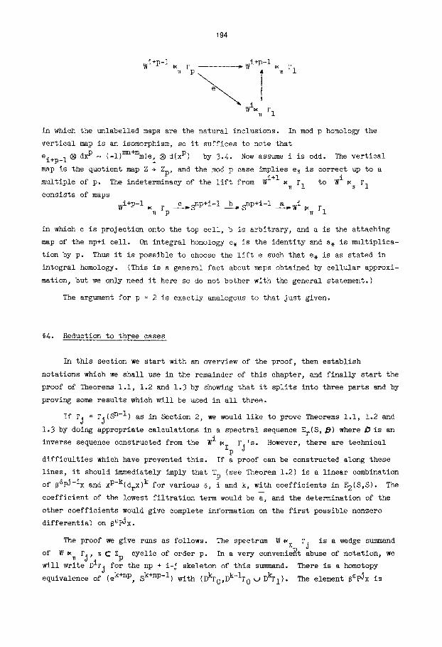
194

W i+p-I ~ F ~ ~+p-I ~ £I

WI~ r I

in which the unlabelled maps are the natural inclusions. In mod p homology the

vertical map is an isomorphism, so it suffices to note that

el+p_ 1 ~ dx p ~ (-l)mn+mm!ei ® d(x p) by 3.4. Now assume i is odd. The vertical

map is the quotient map Z + Zp, and the mod p case implies e, is correct up to a

multiple of p. The indeterminacy of the lift from W i+l ~ F 1 to W i ~ F 1

consists of maps

W i+p-I ~ £p c ~Snp+i-i b,snp+i-i a W i ~ F I

in which c is projection onto the top cell, b is arbitrary, sad a is the attaching

map of the np+i cell. On integral homology c, is the identity and a, is multiplica-

tion by p. Thus it is possible to choose the lift e such that e, is as stated in

integral homology. (This is a general fact about maps obtained by cellular approxi-

mation, but we only need it here so do not bother with the general statement. )

The argument for p = 2 is exactly analogous to that just given.

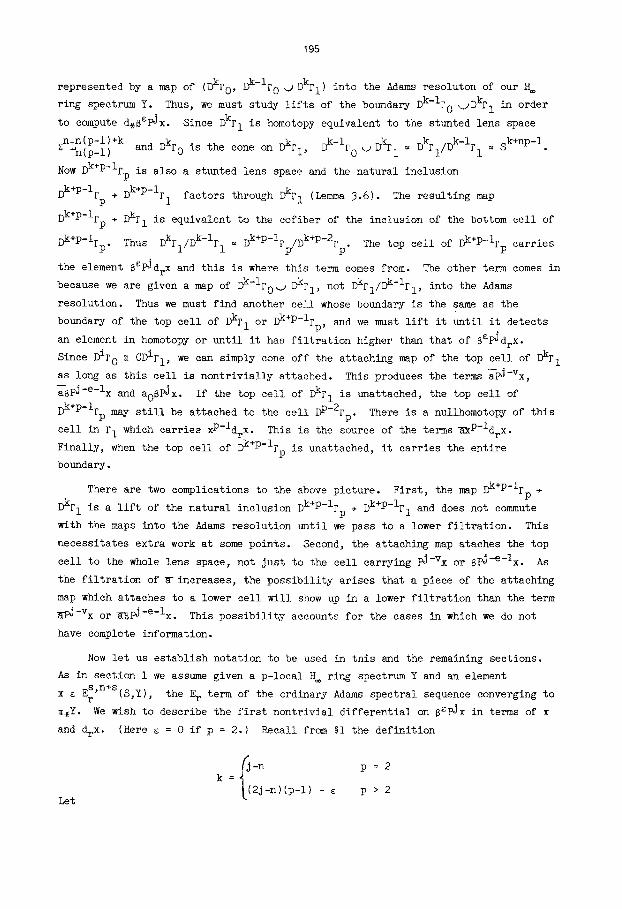
§4. Reduction to three cases

In this section we start with an overview of the proof, then establish

notations which we shall use In the remainder of this chapter, sad finally start the

proof of Theorems 1.1, 1.2 and 1.3 by showing that it splits into three parts and by

proving some results which will be used in all three.

If rj = Fj(S n-l) as in Section 2, we would like to prove Theorems I.I, 1.2 and

1.3 by doing appropriate calculations in a spectral sequence Er(S , ~) where ~ is an

inverse sequence constructed from the wi ~Z £j's. However, there are technical

P difficulties which have prevented this. If a proof can be constructed along these

lines, it should immediately imply that Tp (see Theorem 1.2) is a linear combination

of 66~-ix and xP-k(drx)k for various 6, i and k, with coefficients in E2(S,S). The

coefficient of the lowest filtration term would be a, sad the determination of the

other coefficients would give complete information on the first possible nonzero

differential on 6~x.

The proof we give runs as follows. The spectrum W ~ P is a wedge sun~msad z j

of W ~ P~, ~ C Z~ cyclic of order p. In a very convenient abuse of notation, we

will write D £j for the np + i-j skeleton of this summand. There is a homotopy

equlvalence of-(e k+np, S k+np I) wlth (DkFo,D k I£oUD~I). The element 8S~x is

195

represented by a map of (Dkro , Dk-lr 0 ~ Dkrl ) into the Adams resoluton of our H

ring spectrum Y. Thus, we must study lifts of the boundary Dk-l£o ~Dkrl in order

to compute d,8~x. Since Dkrl is homotopy equivalent to the stunted lens space

znTn(p-l)+k _~ = ~n(p-l) and DkF0 is the cone on Dk£1 , Dk-I£ 0 ~ Dkrl D~I/Dk-IF 1 S k+np-l.

Now Dk+p-IFp is also a stunted lens space and the natural inclusion

Dk+p-IFp ÷ Dk+p-IFI factors through ~F 1 (Lemma 3.6). The resulting map

Dk+p-lrp ÷ DkFI is equivalent to the cofiber of the inclusion of the bottom cell of

Dk+p-IFp. Thus Dkrl/Dk-IFl = Dk+p-IFp/Dk+p-2Fp. The top cell of Dk+p-IFp carries

the element 8e~drx and this is where this term comes from. The other term comes in

because we are given a map of Dk-IF0~ DkFI , not DkFl/Dk-I£1 , into the Adams

resolution. Thus we must find another cell whose boundary is the same as the

boundary of the top cell of ~F 1 or ~+P-lrp, and we must lift it until it detects

an element in homotopy or until it has filtration higher than that of 8e~dr x.

Since DiF0 ~ CDiFI , we can simply cone off the attaching map of the top cell of DkFI

as long as this cell is nontrivially attached. This produces the terms ~-Vx,

~8~-e-lx and aoSPJx. If the top cell of DkF1 is unattached, the top cell of

Dk+p-IFp may still be attached to the cell DP-2Fp. There is a nullhomotopy of this

cell in F 1 which carries xP-ldr x. This is the source of the terms ~P-ldrx.

Finally, when the top cell of Dk+p-IFp is unattached, it carries the entire

boundary.

There are two complications to the above picture. First, the map Dk+p-IFp +

Dk£1 is a lift of the natural inclusion Dk+p-iFp + Dk+p-I£1 and does not commute

with the maps into the Adams resolution until we pass to a lower filtration. This

necessitates extra work at some points. Second, the attaching map ataehes the top

cell to the whole lens space, not just to the cell carrying ~-Vx or 8pj-e-lx. As

the filtration of ~-increases, the possibility arises that a piece of the attaching

map which attaches to a lower cell will show up in a lower filtration than the term

-Vx or ~B~-e-lx. This possibility accounts for the cases in which we do not

have complete information.

Now let us establish notation to be used in this and the remaining sections.

As in section 1 we assume given a p-local ~ ring spectrum Y and an element

x a ErS'n+S(s,Y), the E r term of the ordinary Adams spectral sequence converging to

~,Y. We wish to describe the first nontrivial differential on 8ePJx in terms of x

and drX. (Here e = O if p = 2.) Recall from §I the definition

Let

E =Jj-n p = 2

k [ 2j-n)(p-l) - e p > 2

196

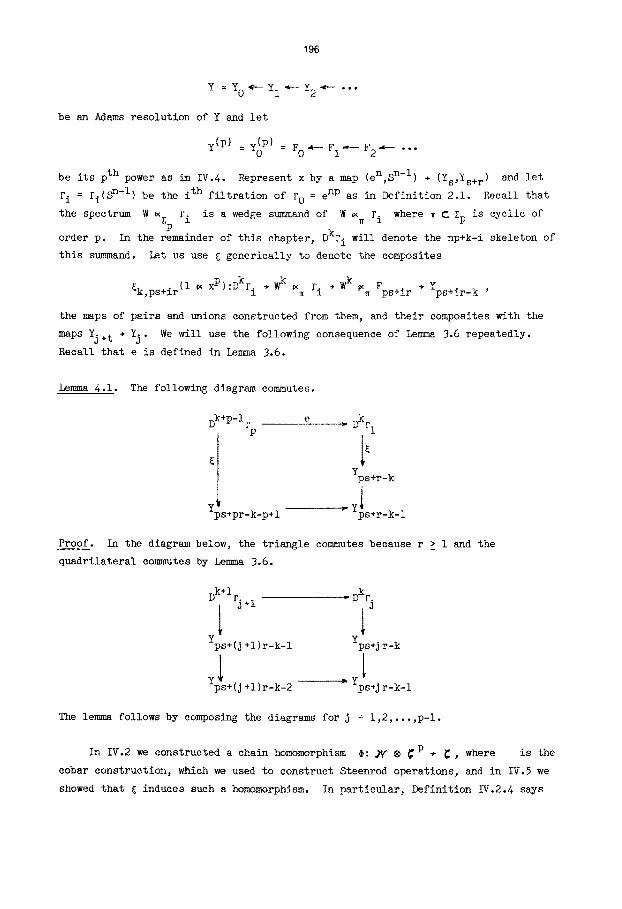
Y = YO~--YI4--Y2 ~- ,..

be an Adams resolution of Y and let

y(P) = y~P) = FO~-- FI~--F2 ....

be its pth power as in IV.4. Represent x by a map (en,s n-l) ÷ (Ys,Ys+r) and let

F i = Fi(S n-l) be the i th filtration of F 0 = e np as in Definition 2.1. Recall that

the spectrum W ~ F i is a wedge sLunmand of W ~ F. where ~ C Zp is cyclic of ~p ~ x

order p. In the remainder of this chapter, DkFi will denote the np+k-i skeleton of

this summand. Let us use ~ generically to denote the composites

~k,ps+ir (I ~ xP):Dkri ÷W k ~ F i + W k ~ ÷ ~ Fps+ir Yps+ir-k '

the maps of pairs and unions constructed from them, and their composites with the

maps Yj+t ÷ Yj" We will use the following consequence of Lemma 3.6 repeatedly.

Recall that e is defined in Lemma 3.6.

Lemma 4.1. The following diagram commutes.

Dk+p-I r e .... ~ Dkrl P

Y p s + r - k

- y l ps+pr-k-p+l r ps+r k 1

Proof. In the diagram below, the triangle commutes because r ~ I and the

quadrilateral commutes by Lemma 3.6.

Dk+IF , ,,. DkF. j+l , 3

L Yps+ (j +l ) r-k-1 Yps+j r-k

Yp!+(j+l)r k 2 " - - ~Yp!+jr-k-i

The lemma follows by composing the diagrams for j = 1,2,...,p-l.

In IV.2 we constructed a chain homomorphism $: 2~ @ ~ p ÷ ~, where is the

cobar construction, which we used to construct Steenrod operations, and in IV.~ we

showed that ~ induces such a homomorphism. In particular, Definition IV.2.4 says

197

and

8~x = (-l)Jv(n)¢,(e k~ x p) p > 2

SqJx = ¢,(ek~x 2) p = 2.

The following relative version of Corollary IV.5.4 gives us maps which represent

these elements. In it we let ~ be the cobar construction C(Zp,~p,H,Y) so that

~s,n+s ~ ~n(Ys/Ys+l) ~ ~n(Ys,Ys+l ) and let ~4 z= C,(W) so that ~'k = Ck(W) £

~k(Wk/w k-l) ~ ~k(Wk,wk-1).

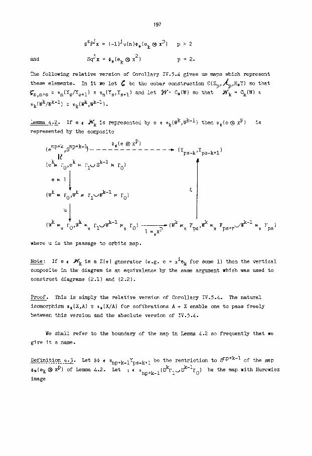
Lemma 4.2.

represented by the composite

(enp+k,snp+k_ ~ $, (e®xp)

(e ~ r o , e k ~ r l ~ , S k-1 ~ r O)

e~l

(W k ~ r 0

U

g

If e ~ ~k is represented by e ~ ~k(Wk,W k-l) then $,(e®x p)

r

,W k ~ rl~JWk-l~ r O)

-~" (Yps_k,Yps_k+l)

is

t

) Fps, Fp +r -i Fps I~ x p ~ ~

w

where u is the passage to orbits map.

Note: If e ~ ~W' k is a Z[~] generator (e.g. e = ~le k for some i) then the vertical

composite in the diagram is an equivalence by the same argument which was used to

construct diagrams (2.1) and (2.2).

Proof. This is simply the relative version of Corollary IV.5.4. The natural

isomorphism ~,(X,A) ~ ~,(X/A) for cofibrations A + X enable one to pass freely

between this version and the absolute version of IV.5.4.

We shall refer to the boundary of the map in Lemma 4.2 so frequently that we

give it a name.

Definition 4.3. Let ~$ E ~np+k_iYps_k+l be the restriction to S np+k-I of the map

#,(e k ~ x p) of Lemma 4.2. Let i E ~np+k_l(DkFl~Dk-lr0 ) be the map with Hurewicz

image

198

(-l)kek®d(xP) +

0 k=0 or k odd, p > 2

0 k+n odd, p = 2

Pek_l®xP 0 / k even, p > 2

i-1)k2ek_l®X2 k+n even, p 2

Lemma 4 . 4 . ( i ) ~$ = ~ , ( t )

(ii) t is an equivalence

(iii) Orienting the top cell of DkF1 correctly, the homotopy class t

contains the map a 3 of diagram (2.2).

Proof (i) holds because we are in the Hurewicz dimension of DkrlkjDk-l£ 0 = Snp+k-I

so the Hurewicz image of I is sufficient to determine t, and its Hurewicz image is

the boundary of the cell ek®XP. Statement (ii) is immediate from the Hurewicz

isomorphism, and statement (iii) is immediate from the fact that a 3 is an

equivalence.

The differentials on 6S~x are given by the successive lifts of (-I) j v(n)~¢

when p > 2, and of S¢ when p = 2. Corollary 2.8 and the discussion following it

show that the attaching maps of lens spaces, and hence elements of Lm J, enter into

the question of lifting this boundary. In the remainder of this section we

establish various facts about the numerical relations between the filtrations and

dimensions involved, the last of which will enable us to split our proof into three

very natural special cases.

Lamina 4.5. If p > 2, the generator of Im J in dimension jq-I has filtration < j.

If p = 2 the generator of Im J in dimension 8a+a (a = 0,1,3,7) has filtration <

4a+~ if ~ I 7, and < 4a+4 if ~ = 7.

P__roof. The vanishing theorem for Ext A (Zp,Zp) says that Ext st = 0 if

O < t-s < U(s), where U(s) = qs-2 if p p 2 and

8a - i ~ = 0

8a+ 1 ~= 1 U ( 4 a + ~ ) =

8a+2 ~=2

8 a + 3 ¢ = 3

i f p = 2 by [4] and [ 5 6 ] . F i r s t suppose p > 2. The Im J g e n e r a t o r i n d imens ion

j q - 1 i s d e t e c t e d by an e lement o f Ex t s , t where t - s = j q - 1 . Hence j q - 1 > U(s) =

sq-2, which implies j > s. Now, suppose p = 2. A trivial calculation shows that if

199

s > 4a + ~, e = 0,1,3,4, then U(s) > 8a + c if e ~ 4, 8a + 7 if e = 4. This

immediately implies the lemma.

We apply this to prove the following three lemmas. As in §l let v be

Vp(k + n(p-1)), and let f be the Adams filtration of the generator of Im J in

~v_l SO.

Lemma 4.6. Assume p > 2. If v = k+l and f ~ r-I then pr-p-k+l < 2r-l.

Proof. Equivalently, we must show k > (p-2)(r-l). By Lemma 4.5

f < v _ k+l - q q

Thus k+l ~ qf ~ q(r-1) and hence it is sufficient to show that

q(r-1) - 1 > (p-2)(r-1). This is immediate since r > 1.

Lemma 4.7. Either min{pr-p+l,v+f} < v+r-I or r = p = 2 and v = i or 2.

Proof. Suppose p > 2. Then f < v/q. If pr-p+l > v+r-1 then

v < (p-1)(r-1) + 1 and hence

r-1 I --< r-l. f_< ~ +q

Now suppose p = 2. We must show that if r ~ v then f < r-1. It suffices to

show f < v-l. This follows from Lemma 4.5 except when v = 1,2, or 4- In these

cases f = 1 so the lemma holds when v = 4. If v =l or 2 then f < r-1 unless

r = 2. This completes the lemma.

Lemma 4.8. Exactly one of the following holds:

(a) v > k + p-l,

(b) v = k+l and if p > 2 then n is even,

(c) v < k.

Proof. There is nothing to prove if p = 2, so assume p > 2. We must show that if

k < v _< k+p-1 then v = k+l and n is even. Recall that k = (2j-n)(p-1)-e and

v = Vp(k+n(p-1)) = Vp(2j(p-1)-a). If a = 0 then v = 1. Hence k = O and n = 2j so

that (b) holds as required. If ~ = 1 then v = q(1 + gp(j)). Dividing the

inequalities k < v < k+p-1 by p-1 yields

1 i 2j-n- ~ < 2(l+~p(j)) < 2j-n - p-i + 1

which has only one solution: 2(1 + ~p(j)) = 2j-n. Hence n is even and

v = q(l+~p(j)) = (2j-n)(p-1) = k+l.

200

Lemma 4.8 is a consequence of the splitting of the mod p lens space into wedge

summands, the summand of interest to us being the Zp extended power of a sphere. To

see the relation, recall that v tells us how far we can compress the attaching map

of the top cell of W k ~ rl zn-1 ~n(p-1)+k = ~n(p-l) When v ~ k, it compresses to

W k-v ~ F 1 and no further. When v > k it is not attached to W k~ r I. However,

recall that there are equivalences

= zn-I ~n(p-l)+k ~ +p-i ~ rp I (n-l)(p-l)

zn-I Tn(P-l)+k W ~ r I = -n(p-l)

by Corollary 2.6, and that the top cell of W k ~ F 1 is the image of the top cell

of W k+p-I ~ Fp by Lemma 3.6. When v > k this cell compresses to W p-2 ~ rp.

The first possibility is that it goes no further, and in this case the wedge summand

of the lens space we are interested in has cells in dimensions n(p-l) and n(p-l)-i

so that n must be even. By the splitting of the lens space into wedge surmmands, the

next possibility is v = k+p-1, which would have the top cell of ~+p-I ~ r P P

attached to the bottom cell. In fact this cannot happen because the attaching map

is in Im J and thus is not in an even stem. So v > k+p-I is the only possibility if + -i

v > k+l, and this says that top cells of W k p ~ Fp.and W ~ ~ r I are unattached.

This "geometry" explains why the differentials on ~S~x are so different in these

three cases. We shall start with the simplest of the three cases, and proceed to

the most complicated.

§5. Case (a): v > k+p-I

Since v > k+p-i ~ i, it follows that s : I if p > 2.

say that

d2r_iPJx = FJdrx if p = 2

• _spj d and dpr_p+lSPJx = r x if p > 2.

Thus Theorems i.I and 1.2

Theorem 1.3 follows automatically from these facts, so these are what we shall

establish.

201

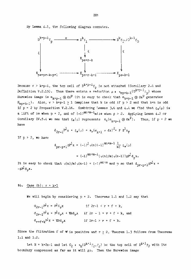
By Lemma 4.1, the following diagram commutes.

e D k+p-I Fp ................... :- DkFI > DkFI ~ D k-I F 0

I s + r - k

Eps+pr-k-p+l ~ Eps+r-k+l "~ Eps-k+l

Because v > k+p-l, the top cell of Dk+p-lrp is not attached (Corollary 2.6 and

Definition V.2.15). Thus there exists a reduction p ~ ~np+k_l(Dk+p-IFp) whose

Hurewicz image is ek+p_l®dxP (it is easy to check that ek+p_lQdxP generates

Hnp+k_l). Also, v > k+p-1 ~ 1 immplies that k is odd if p > 2 and that k+n is odd

if p = 2 by Proposition V.2.16. Combining Lemmas 3.6 and 4.4 we find that ~,(p) is

a lift of 3¢ when p = 2, and of (-l)mn+m-lm!s¢ when p > 2. Applying Lemma 4.2 or

¢,(ek+p_l®dxP). Thus, if p = 2 we Corollary IV.5.4 we see that ~,(p) represents

have

d2r_l~X = ~,(p) = ¢,(ek+ 1

If p > 2, we have

× dx)2= P dJx. r

I dpr_p+16~x = (_i) jv(n)(_l) mn+m-l m-7. ~,(p)

= (-1)mn+m-l(v(n)/m!v(n-l))8~d x. r

It is easy to check that v(n)/m!v(n-1) ~ (-I) nm+m mod p so that dpr_p+lSPJx =

-~drX.

§6. Case (b): v = k+l

We will begin by considering p = 2. Theorems I.i and 1.2 say that

d2r_1~x = ~drX d2r_l~X = ~drX +~drX

dr+f+k~X =WXdrX

if 2r-I < r + f + k,

if 2r - 1 = r + f + k, and

if 2r-i > r + f + k.

Since the filtration f of~ris positive mud r ~ 2, Theorem 1.3 follows from Theorems

1.1 and 1.2.

Let N = k+2n-1 and let C 2 ~ ~N(Dk+lF2,F2 ) be the top cell of Dk+lr2 with its

boundary compressed as far as it will go. Then the Hurewlcz image

202

h(C 2) = ek+l®dX2 and ~C 2 = a = a2(k+n) ~ WN_IF2 £ ~k SO. Since F 2 = S 2n-2 and

rl/r 2 = S 2n-I v S 2n-1 by Lemma 2.2, the Hurewicz homomorphisms in

h ~2n_l(rl,r2) - H2n_l(rl,r 2)

~2n_2r2 ~ H2n_2r 2

are isomorphisms. Let R ~ ~2n_I(FI,F 2) satisfy h(R) = x dx = e0®x dx in the

notation of §3. Then DR ~ ~2n_2F2 is an equivalence since h(8R) = dx 2 = e0®dx2.

Let a also denote (Ca,a) ~ ~N(e2n-l,s2n-2). Let i be the natural inclusion

i:(rl,r 2) ÷ (Dk-lr0,r 2) if k > O and let i = l:(rl,r 2) + (rl,r 2) if k = 0. Let eC 2

denote (e,l),(C 2) ~ ~N(Dkzl,r2 ).

Lemma 6.1: S* = ~,(eC 2 ~ iRa) in ~NY2s_k+l.

Proof. First note that eC2<2 iRa is defined since ~C 2 = S(iRa) = a ~ ~N_IF2 . By

Lemma 4.4, 2¢ = ~,(eC2uJ ira) will follow if eC 2 ~iRa ~ ~N(Dkrl ~ Dk-lr 0) has

Hurewicz image (-1)ke k ® d(x2), since v2(k+n) = k+l implies that either k+n is odd

or k = O. If k ~ 0 then ~:Dkrl~Dk-lF0 + ~F1/Dk-lr I is an equivalence and Lemma

-- ~NDkrl/Dk-lrl 2.7 says that ~(eC 2 ~ ira) = eC 2 ~ since ira factors through

Dk-IF I. Then h(eC--- 2) = e,h(C 2) = (-1)kek® d(x 2) by Len~na J.6 (since k+n is odd)

and we are done. If k = 0 then n is even, since v2(n) = l, and eC 2~jRa ~ ~2n_lrl .

Also, a = - 2E ~2n_2 $2n-2 since h(~C 2) = d(e 1Q dx 2) = (~-l)e 0® dx 2 =

= -2e 0 @ dx 2. To compute h(eC 2 k2Ra), project to rl/r 2 since H2n_lF 1 + H2n_lrl/F 2

is the monomorphism which sends e 0 ® d(x 2) to eo® xdx + eo® dx x. By Lemma 2.7,

Ra) S 2n-1 ~(eC2~ : ÷ F 1 + rl/r 2 equals eC 2 - Ra so

h(~(eC2~Ra)) = h(eC--- 2) - h(~)

= e,(e l® dx 2) + 2eo® xdx

= e 0® (dx)x - e 0~9 xdx + 2e O® xdx

= e 0@ (dx)x + e 0@ xdx.

Therefore h(eC2~Ra) = e0@ d(x 2) and we're done, proving Lemma 6.1.

203

Since ~,SC 2 ~ ~*Y2s+2r, ~*(eC2 ~iRa) = ~,(eC 2) - ~,(iRa) in

~,(Y2s_k+l,Y2s+2r). By Len~na 4.1 (or 3.6), ~,(eC 2) and ~,C 2 have the same image

in ~,(Y2s_k+l,Y2s+2r). Since h(C 2) = ek+l®dX2 , ~,C 2 E ~,(Y2s_k+2r_l,Y2s+2r)

represents ~drX by Lena 4.2. Similarly, h(R) = e0~x dx implies that

~,R E w,(Y2s+r,Y2s+2r) represents XdrX , and hence ~,(Ra) ~ ~,(Y2s+r+f,Y2s+2r)

represents ~'XdrX. This completes case (b) when p = 2.

When p > 2 (and v = k+l) we will treat k = 0 and k > 0 separately. First

suppose k = O. Then v = I, n = 2j and ~ = 0. Also, f = l, [ = a 0 ~ E I'I(s,s) and

a E ~0 S is the map of degree p. Thus, we must show

dr+lXP = aoxP-ldrx.

Heuristically this is exactly what one would expect from the fact that drxP =

p(xP-ldrx). That this is too casual is shown by the fact that we have just proved

(for p = 2) that

d3x2 = h0xd2x + pUd2x.

The extra term arises because when we lift the map representing 2xd2x to the next

filtration, we find also the map representing pnd2x which we added in order to

replace xd2x + (d2x)x by 2xd2x. Thus, our task for p > 2 is to show the analogous

elements can always be lifted to a higher filtration than that in which aoxP-ldrX

lies. The following lemma will do this for us.

Lemma 6.2. There exists elements

Y E ~np_l(Dlr2,r2~2Dlr3)

z , ~np_I(D2F),DIF3~jD2F4)

C 1 c ~np_iFl

X E~np_I(FI,F 2)

such that

C 1 = pX + pY + Z in Wnp_I(DIFI~.,D2F2,F2k_yDIF3~D2F4 ) ,

h(C I) = eo~d(xP) , and

h(X) = eo~xP-ldx.

Proof. Since np-I is the Hurewicz dimension of all the spectra or pairs of spectra

involved, we may define C1,X,Y and Z by their Hurewicz images. Thus C I and X are

given, and we let

1 I h(Y) = ~ e I @ Qd(xP-l)dx - ~ e l@ tp_ 2 , and

1 h(Z) = - m-7 e2 ~ Ntp-3 "

m 2i As in section 3, N = [ s ~ ~ and Q = (s+l) [ is We also let M = [ is ~-i-I ~ and

i=l

204

note that M(a-l) = N-p. Define

1 C = ~ (Mel~tp_ I + e2®tp_ 2) + ~ e l~ Qx p-I dx

in C,(D1£1 ~ D2r2,Fl~jDlr2~D2r3). By Lemma 3.2 it follows that

d(C) = h(C I) -ph(X) - ph(Y) - h(Z)

which shows that C 1 = pX + pY + Z.

By Lemmas 4.4 and 6.2, ~¢ ~ ~*Yps+l is the image of ~,C 1 ~ ~*Yps+r"

also implies that

~,C 1 = p~,X + p~,Y + £,Z

Lemma 6.2

in ~,(Yps+r_l,Yps+2r). Since ~,Y e ,,(Yps+2r_l,Yps+2r) and

~,Z ~ ~,(Yps+3r_2,Yps+3r_l) it follows that ~,C 1 = p~,X in ~,(Yps+r_l,Yps+2r) and

that 8¢ = p£,X in ~,(Yps+l,Yps+2r). Lemma 4.2 implies that

~,X , ~,(Yps+r,Yps+2r) represents xP-ldrx and hence p~,X lifts to ~,(Yps+r+l,Yps+2r)

where it represents a0xP-ldrx. Finally, IV.3.1 implies

dr+l~X = dr+ixP = a0xP-ldrx.

Now suppose that k > O. Then v = k+l is greater than 1 and hence congruent to

0 mod 2(p-l) by V.2.16. Also by V.2.16, e = 1 and k = (2j-n)(p-l)-e is therefore

odd. Lemma 4.4 then implies ~¢ = ~,(t) with h(1) = -ek@ d(xP). The n@xt three

lemmas describe the pieces into which we will decompose 8¢. In the first we define

an element of ~np-i of the cofiber of e:DP-2Fp + FI, which we think of as an element

of a relative group ~np_l(Fi,DP-2rp). In order to specify the image of such an

element under the Hurewicz homomorphism, we use the cellular chains of the cofiber

in the guise of the mapping cone of e,:c,DP-2Fp + C,F I. That is, we let

Ci(rl,DP-2£p) = Ci£1~ Ci_IDP-2Fp

with d(a,b) = (d(a) - e,(b), - d(b)).

Len~na 6.3. There exists R ~ ~np_l(rl,Dp-2rp) such that

(i) h(R) = ((-l)m-leo•tp_l, ep_2®t 0) ~ H,(rl,DP-2rp)

(ii) h(sR) = ep_2~gt 0 = ep_2® (dx) p, and

(lii) 8R ~ ~np_2DP-2rp is an equivalence.

205

Proof. Since d(eo® tp_ l) = Te0® tp_ 2 by Lemma 3.2 and e,(ep_ 2 ® t O ) =

(-1)m-lTe0®tp_2 by Lemma 3.6.(iii), and since d(ep_2®t 0) = 0, it follows that

((-1)meo®tp_l,ep_2®t O) is a cycle of (F1,DP-2rp). Since r I = S np-1 and

DP-2£ = S np-2 , the Hurewicz homomorphism is onto and R satisfying (i) exists. Now

P

(ii) is obvious since the boundary homomorphism simply projects onto the second

factor. Part (iii) is irmnediate from the fact that ep_2@t 0 generates Knp_2DP-2rp.

Now we split R into a piece we want and another piece modulo r 2.

Lemma 6.4. There exist X ~ ~np_l(Fi,F2) and Y ~ ~np_l(Dlr2,r2 ) such that

(i) h(X) = (-1)m-lm!e0®xP-ldx, and

(ii) (i,e),(R) = i,X + j,Y in n,(Dlrl,r2 ) where

i:r I + Dlr l , j:D1F2 * Dlr l and e:I)P-2rp ÷ r 2.

Proof. We are working in the Hurewicz dimension of all the pairs involved so it

suffices to work in homology. We define X by (i) and define Y by

h(Y) = (-l)m-l(m-l)!el ® Qd(xP-1)dx.

On cellular chains, the map (i,e):(F1,DP-2rp) + (Dlrl,F2) induces the homomorphism

i. Ckr l®Ck_lDP-2rp ~ Ckr I - ~ CkD1r I ~ CkDlrl/Ckr 2

in which the unlabelled maps are the obvious quotient maps. Thus, denoting

equivalence classes by representative elements,

h((i,e),R) = ( - 1 ) m - l e 0 ® t p _ l

= (_l)m-lm!e0®xP-ldx + (-1)m-l(m-1)!Te0 ® QxP-ldx

by Lemma 3.2. Since

d(e I ®QxP-ldx) = Teo® QxP-ldx _ el®Qd(xP-1)dx,

it follows that h((i,e),R) = h(i,X + j,Y).

In our last lemma we split ~ into two pieces modulo DP-2rp. Let N = k+np-l.

Lemma 6.5. If v = k+l and k > O, and if Cp ~ ~N(Dk+p-IFp,DP-2Fp) is the top cell

(h(Cp) = ek+p_ l ® dx p) with its boundary compressed as far as possible, then 8Cp =

206

~Ra in ~N_IDP-2rp and

I ~¢ = (-l)m-i ~! ~,(eCp~iRa) in ~*Ys-k+l "

Proof. Since v = k+l, the attaching map of the top cell factors through DP-2rp.

Since 3R is an equivalence by Lemma 6.3.(Iii), the definition of a = ap(k+n(p-1))

ensures that 3Cp = (~R)a = ~Ra. Now Dkrl~Dk-lro = Dkrl/Dk-lr I and, since k > O,

Ha factors through £ 1 C Dk-lr I. Hence, ~ H.(DkFI~jDk-IFo ),

h(eOpu~iRa) = h(eCp)

= e,(ek+p_ l ® dx p)

m = (-I) m!e k® d(x p)

by Lemma 3.6 (since k is odd and n is even). By Lemma 4.4, it follows that 3¢ = (-1) m-1 1 ~.I ~,(eCp<] iRa).

We are now ready to prove Theorems l.l, 1.2, and 1.3 in this remaining case

(p > 2, v = k+l, and k > 0). We must show that

d,B~x = -B~drX $ (-i) e a xP-ldr x.

By Lemma 6.5, d,6~x is obtained by lifting

• i (-l)Jv(n)3¢ = (-l)J+m-lv(n) ~. ~,(eCpu~iRa)

from ~,(Yps_k+l ) to the highest filtration possible. Since g,(eCp) and £,(iRa) have

common boundary in Yps+pr-p+2, ~,(eCp<jiRa) = ~,(eCp) - ~,(iRa) in

w,(Yps_k+l,Yps+pr_p+2). By naturality of ~, ~,(iRa) is the image of

E ~,(Y + ,Y + +~) ~,Ra psr ps pr-p z

and by Lemma 4.1, ~,(eCp) is the image of

~,Cp e ~,(Yps+pr_k_p+l,Yps+pr_p+2).

Lemma 6.4 implies that ~,R = ~,X in ~,(Yps+r_l,Yps+2r_l) since ~,Y is in filtration

2r-1 or higher. (Note that since @R is mapped into r 2 by e in 6.4.{ii), Lemma 4.1

forces us to work modulo filtration 2r-l, the filtration into which ~ maps DIF2 .)

Thus

~,(eCpK_JiRa) = ~,% - ~,Xa in ~,(Ys_k+l,Yps+2r_l),

and, since~has filtration f, ~,Xa comes from ~,(Yps+r+f,Yps+2r). By Lemma 4.6,

either r+f or pr-k-p+l is less than 2r-l, so that at least one of ~,Cp and ~,Xa is

nontrivial in w,(Yps_k+l,Yps+2r_l) in general. Since h(Cp) = ek+p_l• dx p and

h(X) = (-1) m-1 m!eo@ xP-ldx, Lemma 4.2 implies that

207

~,Cp represents (-i) j I 8~dr x v(n-l)

~,Xa represents (-l)m-lmE axP-ldr x.

It then follows that

and

d,8~x = (-l)Jv(n)~

I - ~,Xa) = (-l)J+m-lv(n) ~ (~,Cp

v(n) I 8~dr x _ (_l)Jv(n) ~ xP-ldrx = (-l)m-i "~(n-l) m!

: - 8~drX $ (-i) e a xP-ldr x

since v(n)/v(n-l) =_ (-i) m m! (mod p) and since v = k+l implies 2(e+l)(p-l) =

(2j-n)(p-l) so that n = 2(j-e-l) and hence

-(-l)Jv(n) = (_l)J+l(_l)J-e-i = (_i) e.

This completes case (b).

§7. Case (c): v < k.

In this case the boundary ~ splits Into a piece which represents the same

operation (~ or Bg~) on drX and another piece which is an operation of lower

degree applied to x times an attaching map of a stunted lens space. We begin with

the lemma needed to identify this latter piece exactly. Recall the spectral

sequence of IV.6, and recall the notations established in §l.

~k-v~n(p) be the attaching map of the top cell of Lemma 7.1. Let ~ ~ ~k+np_l u o

Dks n(p) and let f be the filtration of p,(a) = ap(k+n(p-1)), where p:Dk-Vs n(p) +

S k+np-v is projection onto the top cell. Let ~)be the sequence

Dk-Vsn(P) + Dk-V-iSn(P) ..... Sn(P).

In the spectral sequence Er(S,~)) the following hold:

(a)

(b)

1 ~ filt(~) ~ f,

if filt(a) = f then ~ is detected by

k-v-I aek_ v + [ c.e.

i=O I z

for some c i ~ E2(S,S) ,

208

(c) if p : 2 and v ~ I0 or p > 2 and v ~ pq then filt(a) = f

and a is detected by aek_ v.

Proof. (a) Since ~, = 0 in mod p homology, filt(e) > O. Note that this fact

(applied to all the attaching maps of Dk-Vs n(p)) ensures that the spectral sequence

can be constructed. Since p induces a homomorphism from Er(S,~) to Er(S,S) , and

p,(~) has filtration f, a must have filtration J f.

(b) By IV.6.1(i), every element has the fo~

k-v c.e. ll

i=0

for some c i. If filt(~) = f then the element detecting a projects to K in the ~ams

spectr~ sequence of the top cell. Hence Ck_ v = K. (In fact this argument shows

that if Ck_ v i 0 then filt(~) = f and Ck_ v = ~.)

(c) Under the stated hypothesis, ~ek_ v is the only element of filtration ~ f

in degree k+np-l.

To prove Theorems i.i, 1.2 and 1.3, let us first assume that v = I. Then k is

even and ~ = 0 if p > 2, and k+n is even if p = 2. Theorems 1.1 and 1.2 say that

d2~x = h0~-ix if p : 2, and

d2~x = aOS~X if p > 2.

Theorem 1.3 follows from Theorems i.I and 1.2 in this ease. The first step is to

split the element I of Definition 4.3 into two pieces. Recall that

(-l)k(e k @ d(x p) + Pek_ 1 × x p). h( i)

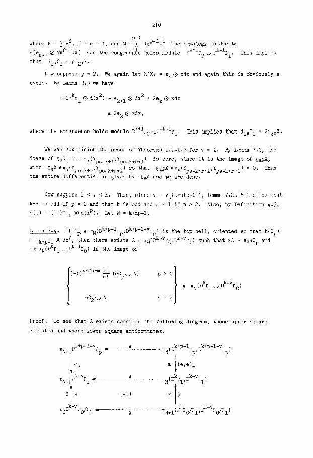
Lemma 7.2: If k > v = i and C E ~ (DkF ,Dk-IF ) is the top cell, oriented so . . . . 1 k+np-1 1 1 k k i that h(C I) = (-l)kek ® d(xP), there exists A( ~k+np_l(D -ir0,D - F I) such that

h(A) = (-l)k-lpek_l ®x p

and i = CI~A~ ~k+np_l(DkFl ~ Dk-lr0).

Proof. Let N = k+np-l. To see that A exists, consider the boundary maps and

Hurewicz homomorphisms

~N ( Dk-I To' Dk-I Fl )

h

=

HN( D k-I FO, D k-I F 1 )

,. ~N_IDk-IFI -~

h

HN_IDk-IFI

~N ( DkFI ' Dk-I FI )

HN( Dkrl, D k-I r I )

209

The isomorphisms are isomorphisms because Dk-IF 0 = * by Lemma 2.4 and because

DkFI/Dk-IFI = S k+np-l. Certainly A exists satisfying ~A = 8C 1. It follows that

~(h(A)) = :~(h(Cl)) = ~((-1)k-lpek_l®xP),

showing that h(A) = (-1)k-lpek_ 1 ® x p.

To show that ~ = Cl~ A, it is enough to show h(t) = h(C 1 ~A), since

Dk~ 1 ~ Dk-l~ 0 = S k+np-1. With N = k+np-1, note that HNDk-IF1 = 0. This implies

that the homomorphism

i, HN~Fl~j Dk-l? 0 = HN(Dk~l ~ Dk-i F0, Dk-lrl )

is injective, so that we need only show i,h(~) = i,h(Cl~J A). By Lemma 2.7,

i,h(C 1 ~A) = h(C l) -h(A) and the result follows.

We now have 3~ = ~,l = ~,(Cl~J A) = ~,C l - ~,A modulo Yps+r-k+l since

£*(Dk-IFI) ~ Ys+r-k+l" Applying Lemma 7.1 we find that ~,A represents

(-1)k-la0$,(ek_ 1 ® x p) in ~,(Yps_k+2,Yps+r_k+l) (with a 0 = h 0 if p = 2). Sorting

out the constants, we find using Definition IV.2.4 that -~A contributes aO~X , if

p > 2, and ho~-lx , if p = 2, to the differential on ~x. Thus, it remains only to

show that ~,C 1 is in a higher filtration than ~,A.

Lemma 7.J. If i I and i 2 are the maps

( DkF1 ,Dk-irl

Dk+IF2 )

then there exists X such that il,C I = P(i2,X).

Proof. Since k+np-1 is the Hurewicz dimension of the domain and codomain of i2, it

suffices to work in homology. First suppose p > 2. We let h(X) = e k ® xP-ldx,

which is obviously a cycle modulo Dk-lr I ~_s DkF2 • Then, in the codomain of i I and i 2

we have

e k@d(x p) = e k® NxP-ldx

= Te k®Mxp-ldx + pe k® xP-ldx

~ ek+ 1 • M-Id(x p-l)dx + pe k @ xP-ldx

- p e k ® xP-ldx,

210

p-I where N = ~ i, T = ~ - i, and M = ~ i~P-i. I The homology is due to

d(ek+ I ® MxP-ldx) and the congruenle holds modulo Dk+IF2 ~_J Dk-lr I. This implies

that il,C I = Pi2,X.

Now suppose p = 2. We again let h(X) = e k ® xdx and again this is obviously a

cycle. By Lemma 3.3 we have

(-l)kek®d(x 2) ~ ek+ I ® dx 2 + 2e k® xdx

2ek®Xdx ,

where the congruence holds modulo Dk+iF2~jDk-lrl . This implies that il,C 1 = 2i2,X.

We can now finish the proof of Theorems 1.1-1.3 for v = I. By Lemma 7.3, the

image of ~,C I in ~,(Yps_k+l,Yps_k+r+l) is zero, since it is the image of ~,pX,

with ~,X E ~,(Yps_k+r,Yps_k+r+l) so that ~,pX~,(Yps_k+r+l,%s_k+r+ I) = O. Thus

the entire differential is given by -~,A and we are done.

Now suppose I < v < k. Then, since v = Vp(k+n(p-l)), Lemma V.2.16 implies that

k+n is odd if p = 2 and that k is odd and e = i if p > 2. Also, by Definition 4.3,

h(1) = (-1)kek®d(xP). Let N = k+np-1.

Lemma 7.4. If Cp ~ ~N(Dk+p-IFp,Dk+p-I-VFp) is the top cell, oriented so that h(Cp)

= ek+p_ I ® dx p, then there exists A ~ ~N(Dk-Vro,Dk-Vrl ) such that ~A = e,~Cp and

E ~N(Dkfll ~ Dk-IFo) is the image of

I( _i ) k+mn+m 1 m-T (eCp,j A)

eC 2 <2 A p=

, ~rN(Okr I ,~ D~-Vro )

Proof. To see that A exists consider the following diagram, whose upper square

commutes and whose lower square anticommutes.

~N_IDk+p-I-VI~p .: 8 ~N (Dk+p-IFp,Dk+p-l-VFp)

i e, -- I(e,e),

~N_IDk-VFI ~ ~ ~N(Dkrl ,Dk-VF I )

~NDk-Vro/rl _, ~ -- ~N÷l(DkrO/r l ,Dk-Vro/ r l )

211

The isomorphisms are isomorphisms because Dkr0 = * = Dk-Vr0 by Lemma 2.4 and (e,e)

is an equivalence by Lemma 3.6. Thus, we may define A = 8-1e,SCp. To see that I is

the image of the claimed elements, it suffices to work in homology, as in Lemma 7.2.

Here, h(eCp~A) = e,h(Cp) - h(A) = e,h(Cp) since HN_IDk-VFI = 0 for dimensional

reasons. By hypothesis, h(Cp) = ek+p_l®dxP , so

h(eCp~A) =

(-l)mn+mm!ek ® d(x p) p>2

(-l)kek ~ d(x 2) p = 2

by Lemma 3.6.

Now,

Comparing this with h(1) = (-l)ke k ® d(x p) finishes the proof.

I (-l)3v(n)~,~ p > 2

d,~aP j x =

~,l p = 2

so, up to a scalar multiple, our differential is ~,(eCp <) A) ~ ~NYps_k+l. By

Corollary 2.8 and Lemma 4.1 we find that

~,(eCpk2A) = ~,eCp - ~,A in WN(Yps_k+l,Yps_k+r+v)

= ~,Cp - ~,A in ~N(Yps_k+l,Yps_k+r+v_l).

It follows from the definition of Cp that ~,Cp lifts to ~*(Yps-k+p.-pr +l,Yps-k+r+v )"

By Lem~a 4.2, ~,Cp represents ~,(ek+p_l® dxP), which equals B~PUdr x up to a

scalar multiple. When p = 2 this shows that ~,C 2 contributes ~drX to d,~x. When

p > 2, the coefficient of 6~drX is

(_i) 2j +k+mn+m ~(n) 1 ~(n-l) m! e --i (rood p).

The congruence follows from the definition of ~, ~(2a+b) = (-1)a(m!)b if b = 0 or l,

and the congruence (m!)2 ~ (_l)m-1 (mod p). This almost proves Theorem 1.1, with

Tp consisting of -~,A ~ WN(Yps_k+l,Yps_k+r+v) plus a possible "error term" in

~N(Yps_k+r+v_l,Yps_k+r+v) coming from the use of Lemma 4.1 above. "Almost" because

this decomposition is only valid modulo filtration ps-k+r+v and we must still show

that either ~e~drX or Tp will be a filtration lower than this in order to finish

the proof of Theorem 1.1. To do this, we must identify ~,A. Referring to the

212

diagram in the proof of Lemma 7.4, the element Cp in the upper right corner goes to

A in the lower left corner if we follow the top and left arrows, while it goes to

(-l)k+mu+mm!a p > 2

p = 2,

where e is the attaching map of the cell ek®xP , if we follow the bottom and right

arrows. Since the lower square anticommutes and since k is odd if p > 2, it follows

that ~ (-l)mn+mmla p > 2

A =

-~ p = 2.

Applying Lemma 7.1(a) we see that ~,A has filtration less than or equal to ps-k+v+f.

Lemma 4.7 implies that, unless r = p = 2 and v =l or 2, one of ~,Cp and ~,A will

occur in a filtration less than ps-k+v+r-1. Thus Theorem 1.1 is proved unless

r = p = v = 2 (since v = 1 has already been dealt with). Applying the rest of Lemma

7.1 we find that

~,A = I (-l)mn+mm! ~¢*(ek-v~xP) P > 2

l -a¢,(ek_v(~X2) p = 2

v = k (since Dk'VF0/rl = S n(p) has only one cell in this case) or if p = 2 and if

v ~ l0 or if p > 2 and v ~ pq. Combining constants, we find that T 2 = a~-Vx and

that Tp = (-1) e-l a~-e-lx if p > 2 (recall that e = ~p(j )). The constant in the

odd primary case comes from the fact that v = Vp(k+n(p-1)) = Vp(2j(p-1) - l) =

2(p-1)(l+e) by V.2.16, so k-v = (2(j-e-l) - n)(p-1) - 1. This completes the proof

of Theorem 1.2 except when r = p = v = 2 (as noted above) or when pr-p < v < k. In

the latter case, Lemma 7.1.(a) still ensures us that

filt(~,A) ~ ps-k + v+l

> ps-k + pr - p+l

= filt(~,Cp).

Hence the term contributed to d,~S~x by ~,Cp appears alone in this case. This

completes the proof of Theorem 1.2 except when r = p = v = 2. Deferring the latter

case until the end, we shall now prove Theorem 1.3. If p = 2 we may assume v > 8,

while if p > 2 we may assume v > q. The attaching map ~ of Lemma 7.1 must then have

filtration 2 or more. This is so because

(i) all but the top two cells are in filtration 2 or more,

213

(ii) the next to top cell component is the product of a positive dimensional

element of E2(S,S) (since v > 0) and a cell in filtration l, so has

filtration at least 2,

(iii) the top cell component is a permanent cycle (being the image of the

permanent cycle a), hence has filtration at least 2 by the nonexistence

of Hopf invariant one elements in dimension v-1.

This implies that ~,A has filtration ps-k + v+2 or more. Since ~,Cp has filtration

ps-k + pr - p+l and ~ splits into these pieces modulo filtration ps-k + r +v-l, we

di6a~x = 0 if have

i ~ min{v+l,pr-p,v+r-2}

= min(v+l,pr-p} ,

the equality holding because v+r-2 < v+l implies r = 2, so that pr-p = p < v = v+r-2

by our assumption on v. This proves Theorem 1.3.

It remains only to prove Theorems 1.1 and 1.2 when r = p = v = 2. Together,

they say d3~x = ~d2x + hl~-2x. Let N = k+2n-1 and let C 1 ~ ~N(Dkrl,Dk-2rl ) and

C 2 E ~N(Dk+lr2,Dk-lr2 ) be the top cells, oriented so that h(C l) = (-1)kek ® d(x 2)

and h(C 2) = ek+l®dX2.

Lemma 7.5. There exists A E ~N(Dk-2ro,Dk-2rl ) such that ~A = ~C 1 and

i = Cl~JA in ~N(DkFl~Dk-lr0 ).

Proof. Since Dk-2r0 = * we may define A = 8-1~C 1

=N(Okrl,Dk-2rl ) ~. =N_iok-2rl ~ ~N(Ok-2ro,Dk-2rl ).

Clearly, h(A) = 0, so h(CI~JA) = h(C I) = h(~). Thus i = CI~JA.

It follows that

2¢ = ~,~ = ~,(CI~JA) = ~,C I - ~,A ~ ~N(Y2s_k+l,Y2s_k+4).

As before, we wish to replace ~,C 1 by ~,C 2 plus an error term which we can ignore.

The following lemma is what we need in order to do this.

Lemma 7.6. Let il:Dk-2r I + Dk-lr 2 ~Dk-2rl,

i2:Dk-lr 2 + Dk-IF2~jDk-2FI,

and j:Dk-lr I ÷ Dk£1

214

be the natural inclusions. Then there exists X 4 WN(Dk-lrl,Dk-lr2 ~Dk-2r I)

positive filtration in the Adams spectral sequence, such that in

~N(Dkrl,Dk-lr2~Dk-2rl )

Proof. Since

need only show

satisfying

with

(l,il),C I = (e,i2),C 2 + (j,I),X

p:(Dkrl,Dk-2Fl~jDk-lr2 ) + (DkFi,Dk-lrl) is the cofiber of (j,l), we

p,(l,il),C I = p,(e,i2),C 2 in order to establish the existence of X

(l,il),C I = (e,i2),C 2 + (j,I),X.

The filtration of X is necessarily positive because

D~-lr/o~-Ir2 ~o~-2r I ~ V s ~-I

by I.i.3 and Lemma 2.2. Since N is the Hurewicz dimension of (Dkrl,Dk-lrl) it

suffices to show h(p,(e,i2),C 2) = h(p,(l,il),Cl). This is immediate from Lemma 3.6.

With Le~ma 7.6 we can now finish the proof of Theorems 1.1 and 1.2. The

element ~X is in ~N(Y2s_k+3,Y2s_k+4), but since X has filtration greater than O,

~,X = O in ~N(Y2s_k÷3,Y2s_k+4). Thus ~,C I = ~,(l,il),C I = ~,(e,i2),C 2 in

~N(Y2s_k+2,Y2s_k+4 ). By Lemma 4.1, ~,(e,i2),C 2 = ~,C 2 in ~N(Y2s_k+l,Y2s_k+4), and

~,C 2 lifts to ~N(Y2s_k+3,Y2s_k+4) where it represents ~d2x by Le~na 4.2. Finally,

~,A also lifts to ~N(Y2s_k+3,Y2s_k+4) where it represents hl~-2x by Lemma 7.1.

Thus

d3~x = ~d2x ÷ hl~-2x.