The accuracy of the E, N and P trait estimates: an empirical study using the EPQ-R

The accuracy of the E, N and P trait estimates:an empirical study using the EPQ-R

Pere J. Ferrando*

Universidad ‘Rovira i Virgili’, Facultad de Psicologia, Carretera Valls s/n, 43007 Tarragona, Spain

Received 13 September 2001; received in revised form 22 January 2002; accepted 13 February 2002

Abstract

This study analyzed the responses of 1175 university students to the E, N and P EPQ-R scales and usedItem Response Theory (IRT) (1) to estimate the ‘true’ distribution of the E, N and P traits in this popu-lation, and (2) to assess the measurement accuracy of the E, N and P scale scores over a range of traitvalues. For (1), the results suggested that the distributions of the three traits are unimodal and roughlybell-shaped. The estimated distributions for E and N tended to be symmetrical, but the distribution of Pwas clearly asymmetrical. These results were related to previous studies based on direct scores. For (2) theresults suggested that the precision of the E and N scores is acceptable across a wide range of trait values.However, the P scores provide poor measurement for a large number of subjects in a non-pathologicalpopulation. At the points at which accuracy is maximal, E, N and P scores are reasonably precise accord-ing to IRT standards. However, there is a high degree of uncertainty in the individual estimates which mustbe taken into account when interpreting test scores. # 2002 Elsevier Science Ltd. All rights reserved.

Keywords: Item Response Theory and personality measurement; Conditional standard error of measurement; Relia-bility; Trait distribution

1. Introduction

Since 1990 interest has grown in the application of Item Response Theory (IRT) models tocertain types of personality data (Ozer & Reise, 1994; Reise, 1999). In particular, the reviews (e.g.Reise, 1999; Steinberg & Thissen, 1995) suggest that some IRT models in common use are sui-table for fitting personality items that measure dimensional traits, i.e. traits that are assumed toform a continuum along which people are distributed according to some frequency distribution.

0191-8869/03/$ - see front matter # 2002 Elsevier Science Ltd. All rights reserved.

PI I : S0191-8869(02 )00053-3

Personality and Individual Differences 34 (2003) 665–679

www.elsevier.com/locate/paid

* Tel.: +34-9-77-55-80-75; fax: +34-9-77-55-80-88.

E-mail address: [email protected]

mailto:[email protected]

IRT makes stronger assumptions than descriptive Classical Test Theory (CTT). However, if theseassumptions are met, the results are also stronger.A review of empirical IRT applications in the personality domain shows that most empirical

research has been concentrated on assessing model fit and calibrating the items (Ozer & Reise,1994). The main purposes of most empirical studies have been: (1) to assess whether a given IRTmodel provided a good fit to personality data and (2) to study whether the item parameter esti-mates obtained were meaningful and according to the expectations derived from the theory.These objectives are reasonable when one is trying out the scope of a new methodology.Assessing the fit and calibrating the items are only part of any IRT application. If the model

data fit is good in a reasonably large sample, then the item parameter estimates can be taken asknown and used to score people. The scoring phase addresses some interesting issues. In parti-cular, we can assess: (1) the shape of the distribution of the trait levels in the population ofinterest and (2) the accuracy with which the trait is estimated by the measuring instrument. Thispaper is mainly concerned with these two issues.In my opinion, apart from their psychometric interest, these two objectives are important from

both a theoretical and a practical point of view. However, according to the literature, they do notappear to have received much attention in substantive research. For issue (1), in general,dimensional models are not too concerned with the shape of the distribution of a trait. Stagner(1948) suggested that the distribution of a dimensional personality trait in a given population isexpected to be unimodal. Also, it is generally assumed that this distribution is normal or nearnormal in the population of interest (e.g. Eysenck, 1952, 1992). Indeed, most substantivestudies assess the distribution of the test scores in a given sample. However, the distributionof the test scores and the distribution of the trait are very different things. To see this point,consider that for a given ‘true’ trait distribution, the distribution of the scores that measure thistrait can vary simply by choosing different items with different levels of difficulty and differentdiscriminations.As far as the accuracy of trait estimation is concerned, most personality texts clearly state that

test scores are fallible measures of the trait and that they contain considerable measurement error(e.g. Eysenck & Eysenck, 1985; Stagner, 1948). Also, the ‘Standards for Educational and Psy-chological Testing’ (AERA, APA, & NCME, 1999) state that for each test score, estimates of themeasurement error should be reported. However, the literature clearly shows that this is not theusual practice in applied personality measurement. Most test-based personality studies routinelyreport reliability estimates. However, it is not common practice to construct confidence intervalsaround the test scores that give an idea of the precision of that measurement.This paper has two main purposes: (1) to assess the distribution of the Extraversion (E), Neu-

roticism (N) and Psychoticism (P) dimensions as measured by the EPQ-R and (2) to assess theaccuracy of the E, N and P EPQ-R scores as measures of these traits. Both objectives are referredto the same population of interest: social science university students, i.e. a population made up ofyoung, non-pathological adult subjects with a relatively high level of education.I have based the study on a number of IRT procedures. As these procedures are still not in

common use in personality research they are described in some detail in the next sectionwhich also contains an overview of the most related IRT methods. However, the purpose ofthis study is substantive, not methodological, so, the procedures are mostly explained at aconceptual level.

666 P.J. Ferrando / Personality and Individual Differences 34 (2003) 665–679

1.1. Rationale and procedures

The most characteristic feature of parametric IRT models is that they specify the form of theregression of the item response on the trait in a falsifiable way. More specifically, for binaryscored items, common IRT models define the probability of endorsing an item at a given traitlevel as a function of some item parameters. The line connecting the probabilities of endorsementat different trait levels is the item-trait regression, which, in IRT terminology is known as the‘Item Characteristic Curve’ (ICC). Different models are obtained by assuming different forms forthe ICC and by considering a different number of item parameters. However, once a particularmodel is specified, its suitability for a given set of data can be assessed by conducting a goodnessof fit investigation.To date, the most suitable IRT model for binary scored personality items appears to be the

two-parameter model, usually in its logistic form (2PLM). This choice is based on some ‘a priori’considerations and, especially, on empirical reasons. The ‘a priori’ considerations are: (1) gues-sing is not a relevant factor in personality measurement (which makes it unnecessary to use athree-parameter model); and (2) evidence accumulated over the last 80 years suggests that itemsin conventional personality tests differ in the degree to which they correlate with the trait thatthey measure (which makes the one parameter or Rasch model inapplicable in this case). As forthe empirical reasons, the literature shows that, when 2PLM is applied to binary items thatmeasure dimensional personality traits, it tends to produce good fits and item parameter esti-mates that are meaningful and in accordance with the theoretical expectations (Finch & West,1997; Reise, 1999; Reise & Waller, 1990; Waller Tellegen, McDonald, & Lykken, 1996). As wellas these pragmatic reasons, a more substantive rationale for using the 2PLM for this type of traitsis discussed in Ferrando (2001).2PLM is the model chosen for this study. Its mathematical function is

Pð�Þ ¼eað��bÞ

1þ eað��bÞð1Þ

In words, expression (1) states that the probability that a person with a trait level � will endorsea given personality item depends on: (a) the person’s level of �; (2) the threshold or locationparameter b, which indicates the ICC position; and (3) the item discrimination parameter a,which is proportional to the maximum slope of the ICC.Generally, an IRT model is fitted to a set of data in two phases. The first phase is item cali-

bration, which is carried out in a series of steps. First, the assumptions on which the model isbased (mainly unidimensionality) are tested. Second, the item parameters (a and b in this case) areestimated. Then, using these estimates, the suitability of the model is assessed by conducting agoodness of fit investigation. Finally, if the model fits reasonably well, the item parameter esti-mates can be interpreted and used for further purposes.The second phase is to score the data of the subjects. In the CTT-based approach, the usual test

score is simply the unweighted sum of the items endorsed. This type of score is very simple toobtain and easy to interpret. However, it has the obvious limitation that it assigns the sameweight to all of the items, even when it is acknowledged that some items are more precise measuresof the trait than others.

P.J. Ferrando / Personality and Individual Differences 34 (2003) 665–679 667

In IRT, the usual test score is the individual trait level estimated from the pattern of itemresponses that the individual obtained. The first problem with this type of score is that the scale ofthe trait is arbitrary, because the item and the subject parameters in Eq. (1) can be linearlychanged while the resulting probability remains the same. This problem is avoided by setting ametric for the trait. This is usually the z metric, i.e.: mean zero and variance one. We have alsoused this metric in this study, so, the trait estimates or IRT scores can be interpreted as z scores.This metric is well known by psychologists. Furthermore, IRT scores and direct scores can berelated as follows. If the item parameters a and b are known, expression (1) gives the expectedprobability of item endorsement for a subject with a trait level of �. This probability can also bethought of as the average item score that the subjects with this trait level would obtain. Theaverage test score for these subjects would then simply be the sum of the P’s across all the testitems, which could be interpreted as the raw test score expected for subjects with a trait level of �.So, there is a one to one relationship between each trait level and the test score expected at thislevel (Lord, 1980). In IRT, the line connecting the trait levels to the corresponding expected testscores is called the ‘Test Characteristic Curve’ (TCC).Of the procedures for obtaining IRT scores, in this paper we shall consider estimates obtained using

the principle of Maximum Likelihood (ML). Although ML trait estimation is not a simple process,the central idea is. If the item parameters are taken as fixed and known, the ML IRT test score for agiven subject is the � value that makes the observed sequence of item responses of this subjectappear most likely in light of the particular model used (in this case, 2PLM). The ML score haswell-known large sample properties (in this context large sample refers to the number of test items).In particular, as the test length increases, theML score is distributed normally with a mean equal tothe ‘true’ trait value, and a standard deviation that is a function of the trait level and is obtained asa routine by-product of the estimation process. The standard deviation of the ML score is a stan-dard error of measurement (S.E.M.) and can be interpreted as the standard deviation that the MLtrait estimates would have in a subpopulation of subjects all of which have the same trait level.At this point, we must mention an important difference between the S.E.M. of traditional CTT

and the S.E.M. discussed above. The most conventional CTT approach assumes that the S.E.M.is constant for all test subjects. Therefore, the test is supposed to have the same accuracy at anytrait level, and so, the reliability coefficient suffices as a single index of overall test accuracy. Also,the confidence interval for estimating the accuracy of an individual score has the same width atany ‘true’ test score. On the other hand, in IRT the S.E.M. is a function of the trait level, and so,differs in general throughout the range of trait levels. An example will perhaps make clear whythis is so. Consider a test score obtained as the sum of n binary item scores. This test score has afinite range of values from 0 to n. Now suppose that the test measures a dimensional trait thoughtof as a continuous unlimited variable. Under these conditions the relationship between the testscore and the trait levels cannot be linear. Moreover, for subjects with very large or very smalltrait levels large differences in the trait are needed to achieve small changes in the expected testscore. The test will therefore be less accurate when we are measuring extreme trait levels. Thisrationale is not specific of IRT. In modern CTT it is also acknowledged that the S.E.M. cannotgenerally be constant, and CTT-based procedures for estimating conditional S.E.M. at differentlevels have also been proposed (e.g. Lord, 1984).The use of ML scores together with the estimated S.E.M. has important advantages (at least

theoretically). First, if the test is reasonably long, the conditional distribution of the ML scores is


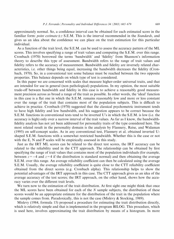
approximately normal. So, a confidence interval can be obtained for each estimated score in thefamiliar form: point estimate�z S.E.M. This is the interval recommended in the Standards, andgives us an idea about the confidence we can place on the trait estimation for this particularindividual.As a function of the trait level, the S.E.M. can be used to assess the accuracy pattern of the ML

scores. This involves specifying a range of trait values and computing the S.E.M. over this range.Cronbach (1970) borrowed the terms ‘bandwidth’ and ‘fidelity’ from Shannon’s informationtheory to describe this type of assessment. Bandwidth refers to the range of trait values andfidelity refers to the accuracy of measurement. Bandwidth and fidelity are inversely related char-acteristics, i.e. other things being equal, increasing the bandwidth decreases the fidelity (Cron-bach, 1970). So, in a conventional test some balance must be reached between the two oppositeproperties. This balance depends on which type of test is considered.In this paper we are concerned with scales that measure higher-order universal traits, and that

are intended for use in general (non pathological) populations. In my opinion, the most suitabletrade-off between bandwidth and fidelity in this case is to achieve a reasonably good measure-ment precision across as broad a range of the trait as possible. In other words, the ‘ideal’ functionin this case is a flat one in which the S.E.M. remains reasonably low and more or less constantover the range of the trait that contains most of the population subjects. This is difficult toachieve in practice. Cronbach (1970) suggested that the classical psychometric instrument tendsto have high fidelity and low bandwidth, and his suggestion appears to be correct because theS.E.M. functions in conventional tests tend to be inverted U’s in which the S.E.M. is low (i.e. theaccuracy is high) only over a narrow interval of the trait values. As far as I know, the bandwidth-fidelity analysis has not yet been addressed for personality traits of the type considered here. Themost related result in the personality domain is the analysis by Flannery, Reise, and Widaman(1995) on self-concept scales. As in any conventional test, Flannery et al. obtained inverted U-shaped S.E.M. functions with a somewhat restricted bandwidth. Whether this is the case or notwith the E, N and P scales will be empirically assessed in this study.Just as the IRT ML scores can be related to the direct test scores, the IRT accuracy can be

related to the reliability used in the CTT approach. The relationship can be obtained by firstspecifying the range of trait values that contains most of the population individuals (for example,between z=�4 and z=4 if the distribution is standard normal) and then obtaining the averageS.E.M. over this range. An average reliability coefficient can then be calculated using the averageS.E.M. Usually, the average reliability coefficient is quite close to the CTT reliability coefficientobtained from the direct scores (e.g. Cronbach alpha). This relationship helps to show thepotential advantages of the IRT approach in this case. The CTT approach gives us an idea of theaverage accuracy of the test scores; the IRT approach, on the other hand, shows how the accu-racy varies over the different trait levels.We turn now to the estimation of the trait distribution. At first sight one might think that once

the ML scores have been obtained for each of the N sample subjects, the distribution of thesescores would be an appropriate estimate for the distribution of the trait in the population wherethe sample comes from. Paradoxically, this is not the case (Mislevy & Stocking, 1989).Mislevy (1984, formula 15) proposed a procedure for estimating the trait distribution directly,

which is relatively simple and that is implemented in the program BILOG. This procedure, whichis used here, involves approximating the trait distribution by means of a histogram. In more


detail, a set of equally spaced points are defined in the region where the bulk of the distribution isexpected to lie, and the relative frequency at each point is estimated by the ML principle. Forexample, if the trait distribution is expected to be approximately standard normal, most of thepopulation subjects will fall between z=�4 and z=4. So, a set of equally spaced intervalsbetween �4 and +4 (the class intervals of the histogram) will be specified, and estimates of therelative frequencies in each of these intervals (i.e. the areas of the corresponding histogram bars)will be obtained.

2. Method

2.1. Participants and procedure

The respondents were 1175 university students (66% women; mean age 21) from the Psychol-ogy and Social Sciences Faculties of the ‘Rovira and Virgili’ University in Tarragona (Spain).Data were collected between the academic years 1991–1992 to 2000–2001.The questionnaireswere completed voluntarily in classroom groups of about 60 students. The instructions givenbefore administration were those printed in the Spanish adaptations of the EPI and EPQ ques-tionnaires.

2.2. Instruments

I used the 100-item Spanish translation of the EPQ-R (Aguilar, Tous, & Andres, 1990). The EPQ-R scales analysed were: Extraversion (E, 23 items), Neuroticism (N, 24 items) and Psychoticism (P,32 items).

3. Analyses and results

3.1. Preliminary results

Because the main purposes of this study were to assess the trait distributions and the measure-ment accuracy of the scales, the results of the early stages of fitting the IRT model will bedescribed only briefly. Additional information and details are available on request.First, the assumption of unidimensionality was assessed by means of nonlinear factor analysis

as implemented in the NOHARM program (Fraser & McDonald, 1988). The results suggestedthat this assumption was adequately met in all three scales. The residuals obtained under the onecommon factor model were low in all cases, and the one factor solution was not improved verymuch by a two-factor model.Next, the 2PLM was fitted using the BILOG 3 program (Mislevy & Bock, 1990). Item para-

meters were estimated by the marginal maximum a posteriori procedure. Using these parameterestimates, the goodness-of-fit of the 2PLM to the data was tested by a chi-squared test of fit sta-tistic for each of the items. The chi-square values were low and nonsignificant for most of theitems in all three scales. I concluded that the 2PLM was appropriate for the present data.


3.2. Estimated latent distributions

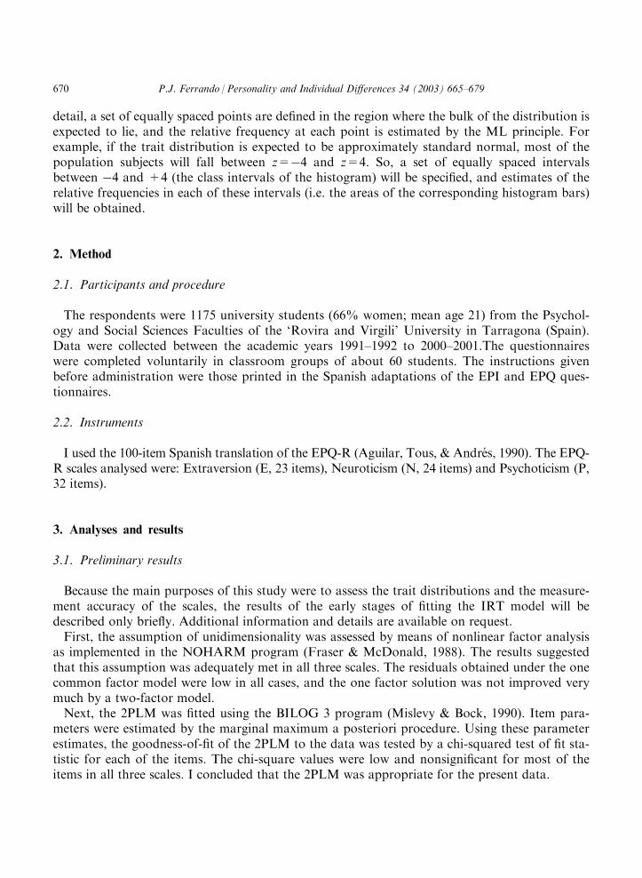
As far as I know, no previous detailed discussions have been provided about the ‘true’ dis-tribution of E, N and P. Eysenck and Eysenck (1976, chap. 5) acknowledged that the test dis-tributions are not necessarily good indicators of the distribution of the underlying trait. However,they made some remarks based on the observed EPQ scores. In summary they said that: (1) in anormal (non-pathological) population, few people are high in P, while many tend to be relativelyhigh in E, and (2) The distribution of N is more spread than that of the other two traits.Fig. 1 shows the estimated trait distributions for E, N, and P from the present data. The dis-

tributions were estimated by Mislevy’s procedure described above using 20 equally spaced pointsbetween �4 and +4. In all three cases the trait was scaled to a z metric (mean 0 and variance 1).As is usually assumed when using the dimensional approach (e.g. Stagner, 1948), the three

estimated trait distributions are unimodal and roughly bell-shaped. The distributions of E and Nare relatively symmetrical. The distribution of E has a slight tendency to concentrate more cases

Fig. 1. Estimated trait distributions: E, N and P.


at the higher end of the continuum (as suggested by Eysenck & Eysenck, 1976), whereas the dis-tribution of N tends to concentrate more cases at the lower end of the continuum. This is anexpected result because N is a more ‘pathological’ dimension than E and our population is ayoung, healthy population of students in which it seems natural for low levels to predominate in N.We turn now to what is usually the most problematical of the three distributions. Eysenck

(1992) suggested that the ‘true’ distribution of P might be inherently asymmetrical in non-pathological populations. However, he also warned that the asymmetry may be due to psycho-metric faults in the P scale (faults which were mitigated in the revised version). The typical dis-tribution of direct P scores is J-shaped, skewed to the right and has strong ‘floor’ effects (Eysenck,Eysenck, & Barrett, 1985). The results of this paper were no exception. The mean of the direct Pscores was 7.35�3.86 (which is quite similar to the one obtained by Eysenck et al. if both sexesare combined), and the form of the distribution was very similar to those displayed in Figs. 1 and2 in Eysenck et al. (1985). In fact, the distribution of the P scale scores was well fitted by a Pois-son distribution (as suggested in Eysenck & Eysenck, 1976).The estimated P distribution in Fig. 1, however, is far less extreme than the distribution of the

direct scores. The ‘floor’ effect disappears and the distribution becomes bell-shaped instead ofJ-shaped. Even so, the estimated P distribution is clearly asymmetrical and concentrates far morecases at the low end of the continuum. This tends to support Eysenck’s suggestion that the dis-tribution of P is inherently asymmetrical in a ‘non-pathological’ population. Eysenck et al. (1985)offer an additional explanation for this asymmetry. High P scorers are uncooperative, andtherefore much less likely to complete a personality questionnaire than low P scorers. So, dis-tributions are likely to be asymmetrical as long as subjects with high P levels are able to decline tocooperate. This point is applicable in this case since EPQ-R was administered entirely voluntarily.

3.3. Accuracy of trait estimates

For the E, N and P scales, the conditional S.E.M. estimates at different trait levels are displayedin Fig. 2.To interpret the results in Fig. 2, we must remember that the traits are scaled with zero mean

and variance unity, and that the estimated distributions of the traits in the population are thosedescribed in the previous section. We can now see that first, the scale scores attain their maximumprecision at different trait levels. Scale E has its point of maximal accuracy at a trait level ofz=�0.87, that is, almost one standard deviation below the mean. The N scale is most precise atz=0.75, and the P scale, the most extreme, reaches maximal accuracy at z=1.88, that is, almosttwo standard deviations above the mean. If we take our population as a reference, this resultmeans that the scales would be more precise in a population with lower levels of E, higher levelsof N, and much higher levels of P. The results for N and P suggest that these scales (especially P)would work better in more ‘pathological’ populations than the one considered here.The second result concerns the degree of accuracy of the different measures. At the trait levels

described above (where the accuracy is maximal), the S.E.M.s are: 0.34 (E), 0.28 (N) and 0.34 (P).Note that these values show that there is a notable degree of uncertainty in the individual esti-mation of trait levels. For example, if a subject has an estimated P level of 1.88, the 95% con-fidence interval for this point estimate is 1.88�1.96 0.34, i.e. (1.22; 2.54), this is an extremely wideinterval even in this the best of cases. This uncertainty seems natural for psychometric instruments


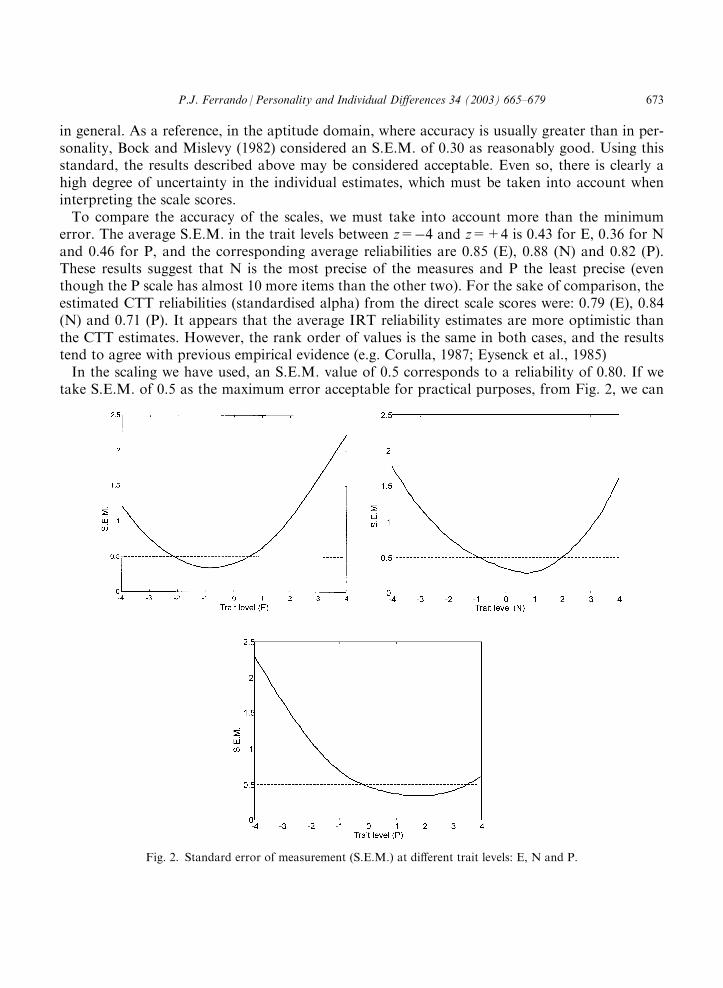
in general. As a reference, in the aptitude domain, where accuracy is usually greater than in per-sonality, Bock and Mislevy (1982) considered an S.E.M. of 0.30 as reasonably good. Using thisstandard, the results described above may be considered acceptable. Even so, there is clearly ahigh degree of uncertainty in the individual estimates, which must be taken into account wheninterpreting the scale scores.To compare the accuracy of the scales, we must take into account more than the minimum

error. The average S.E.M. in the trait levels between z=�4 and z=+4 is 0.43 for E, 0.36 for Nand 0.46 for P, and the corresponding average reliabilities are 0.85 (E), 0.88 (N) and 0.82 (P).These results suggest that N is the most precise of the measures and P the least precise (eventhough the P scale has almost 10 more items than the other two). For the sake of comparison, theestimated CTT reliabilities (standardised alpha) from the direct scale scores were: 0.79 (E), 0.84(N) and 0.71 (P). It appears that the average IRT reliability estimates are more optimistic thanthe CTT estimates. However, the rank order of values is the same in both cases, and the resultstend to agree with previous empirical evidence (e.g. Corulla, 1987; Eysenck et al., 1985)In the scaling we have used, an S.E.M. value of 0.5 corresponds to a reliability of 0.80. If we

take S.E.M. of 0.5 as the maximum error acceptable for practical purposes, from Fig. 2, we can

Fig. 2. Standard error of measurement (S.E.M.) at different trait levels: E, N and P.


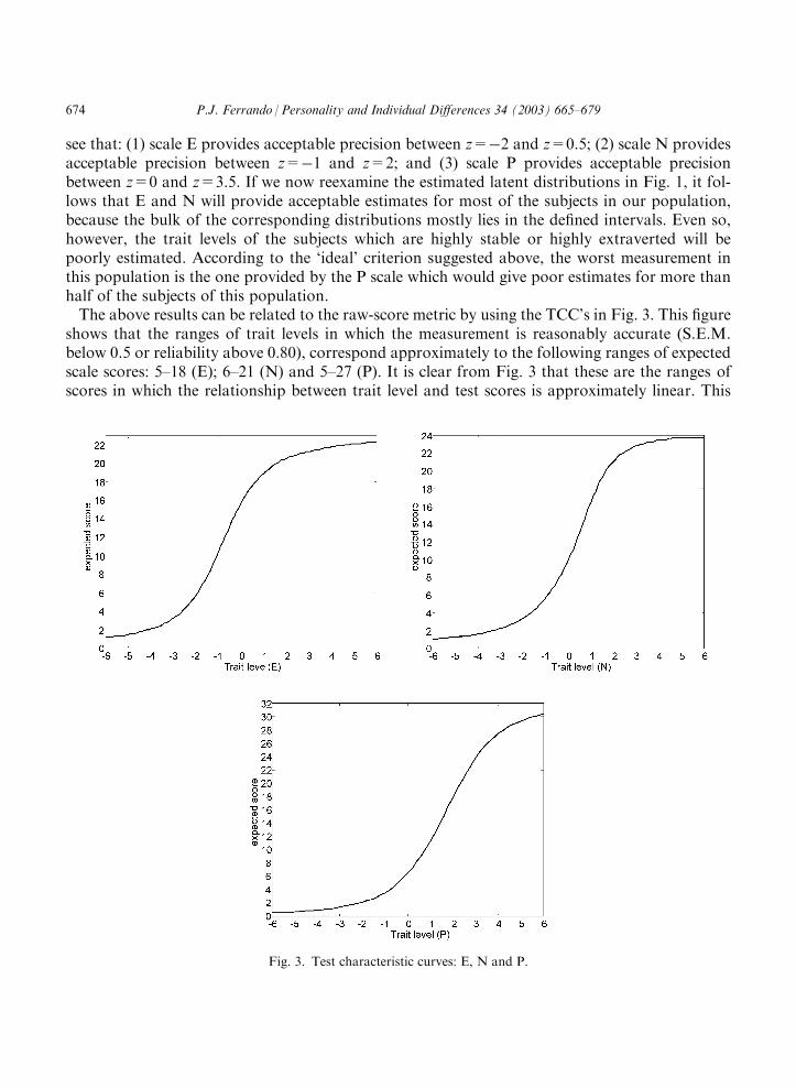
see that: (1) scale E provides acceptable precision between z=�2 and z=0.5; (2) scale N providesacceptable precision between z=�1 and z=2; and (3) scale P provides acceptable precisionbetween z=0 and z=3.5. If we now reexamine the estimated latent distributions in Fig. 1, it fol-lows that E and N will provide acceptable estimates for most of the subjects in our population,because the bulk of the corresponding distributions mostly lies in the defined intervals. Even so,however, the trait levels of the subjects which are highly stable or highly extraverted will bepoorly estimated. According to the ‘ideal’ criterion suggested above, the worst measurement inthis population is the one provided by the P scale which would give poor estimates for more thanhalf of the subjects of this population.The above results can be related to the raw-score metric by using the TCC’s in Fig. 3. This figure

shows that the ranges of trait levels in which the measurement is reasonably accurate (S.E.M.below 0.5 or reliability above 0.80), correspond approximately to the following ranges of expectedscale scores: 5–18 (E); 6–21 (N) and 5–27 (P). It is clear from Fig. 3 that these are the ranges ofscores in which the relationship between trait level and test scores is approximately linear. This

Fig. 3. Test characteristic curves: E, N and P.


information would be useful if the EPQ-R were administered to a participant from this population,and the test was scored conventionally. If the obtained score were outside the above ranges, it couldbe thought that this score would probably be a poor estimate of the corresponding trait level.

3.4. IRT and CTT results: some practical considerations

The test characteristic curves discussed in the section above describe the relations between theCTT metric (expected or true scores) and the IRT metric (trait levels). The applied personalityresearcher might also find it of interest to know what the relation between the estimates of thesescores is. That is to say, the relation between the raw or direct test scores (the estimates of the truescores) and the IRT scores (the estimates of the trait level).Previous empirical studies (e.g. Fan, 1998; Ferrando, 1999) found that correlations between the

CTT raw scores and the IRT scores were very high, usually above 0.95. In the present study, theproduct–moment correlations between these two sets of scores were r=0.96 (E), r=0.97 (N), andr=0.93 (P).The results described above can be expected from the theory. First, any correlation coefficient

(including r) essentially reflects the extent to which the scores are in the same order on bothvariables. Second, under very mild conditions—which any well constructed test usually meets—the raw score is a very good estimate of the order of the respondents (Mokken, 1971). So, bothtypes of scores are expected to be essentially equivalent in terms of the relative scaling of indivi-dual differences, and this is in fact so.Some authors (e.g. Nunnally & Bernstein, 1994) suggested that the extremely high correlation

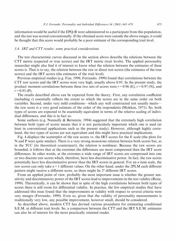
between both types of scores means that it is not particularly important which one is used (atleast in conventional applications such as the present study). However, although highly corre-lated, the two types of scores are not equivalent and this might have practical implications.Fig. 4 displays the scatterplot of the raw scores vs. the IRT scores for the E scale (the plots for

N and P were quite similar). There is a very strong monotone relation between both scores but, asin the TCC (its theoretical counterpart), the relation is nonlinear. Because the raw scores arebounded, it follows that at the extremes the differences are more compressed than the IRT scoredifferences. In other words, at the extremes a wide range of IRT scores are compressed into oneor two discrete raw scores which, therefore, have less discriminative power. In fact, the raw scorespotentially have less discriminative power than the IRT scores in general. For an n item scale, theraw scores can only take n+1 different values. On the other hand, under the 2PLM each differentpattern might receive a different score, so there might be 2n different IRT scores.From an applied point of view, probably the most important issue is whether the greater sen-

sitivity and discriminatory power of the IRT scores lead to improvements in the test validity (Reise,1999). Theoretically, it can be shown that in spite of the high correlations between both types ofscores there is still room for differential validity. In practice, the few empirical studies that haveaddressed this issue found that the improvements in validity with respect to several criteria werevery meagre (Ferrando, 1999). Even so, given that the validity of personality measurements istraditionally very low, any possible improvement, however small, should be considered.As described above, modern CTT has devised various procedures for estimating conditional

S.E.M. at different trait levels. So, a comparison between the CTT and the IRT S.E.M. estimatescan also be of interest for the more practically oriented reader.


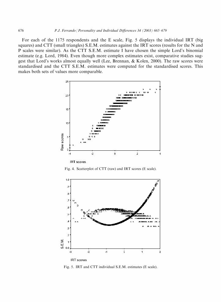
For each of the 1175 respondents and the E scale, Fig. 5 displays the individual IRT (bigsquares) and CTT (small triangles) S.E.M. estimates against the IRT scores (results for the N andP scales were similar). As the CTT S.E.M. estimate I have chosen the simple Lord’s binomialestimate (e.g. Lord, 1984). Even though more complex estimates exist, comparative studies sug-gest that Lord’s works almost equally well (Lee, Brennan, & Kolen, 2000). The raw scores werestandardised and the CTT S.E.M. estimates were computed for the standardised scores. Thismakes both sets of values more comparable.

Fig. 4. Scatterplot of CTT (raw) and IRT scores (E scale).

Fig. 5. IRT and CTT individual S.E.M. estimates (E scale).


Fig. 5 shows a typical phenomenon. At the extreme values of the IRT scores the IRT S.E.M.estimates are arbitrarily large but the CTT S.E.M. estimates are small. This apparent paradox isbecause the raw score is bounded. For example, respondents with a very high trait level (E in thiscase) are virtually certain to obtain a top score on the scale. So, their true score is very close to thetop score on the scale (raw score) and, consequently, their CTT S.E.M. error is almost zero. Inother words, the true score of these respondents can be estimated very accurately. However, theirtrait level cannot because we only know that it is very high but not how high. A similar expla-nation can be used for the other end of the scale.According to the above explanation, what the IRT S.E.M.s show is that we cannot obtain good

estimates for respondents for whom the scale is too ‘easy’ or too ‘difficult’ and that the estimatesare best when the trait levels match the difficulty of the scale. On the other hand, the CTTS.E.M.s essentially reflect the distortions of measurement at the extremes due to the bounded rawscore metric, and can suggest the false conclusion that, at the extremes, the scale measures almostperfectly (see McDonald, 1999, for further discussion).

4. Discussion

The procedures used in this study are not in common use in conventional personalitymeasurement. However, the results suggest that they can obtain information about the measure-ment properties of certain types of personality instruments. Generally we do not obtain thisinformation when we assess the psychometric properties of personality measures by conventionalmethods.According to the present results, the behaviour of the EPQ-R scales is quite acceptable. The

maximal accuracy of the IRT scores is similar to the recommended standards for achievementmeasures, and, for two of the scales, there is reasonably good accuracy over the trait levels thatcontains the bulk of the frequency distribution in our population. However, the scales also haveseveral drawbacks which conventional analysis would not indicate. At a general level, the resultssuggest that the P scale tends to provide poor measurement of a large number of individuals in anon-pathological population. At the individual level, even at the points in which the scores havemaximal accuracy, there is a high degree of uncertainty in the individual trait estimates. It couldbe argued that this problem is inherent to psychometric instruments in general and personalityquestionnaires in particular. Even so, we must take into account this limitation when interpretingtest scores.The main purposes of the present research were to assess the shape of the population and trait

levels, and the accuracy by which the traits are estimated at different levels. For the benefit of themore practically oriented readers I have also compared the individual estimates provided by CTTand IRT, as well as the individual S.E.M. As expected from the theory, the CTT and IRT scoreswere very highly correlated in the three scales, but the relations were nonlinear. Furthermore theIRT scores were shown to be more discriminating than the CTT scores, especially at the extremes.Whether this might improve validity inferences is unclear at present, but I believe that it deservesfurther research.Some previous empirical studies of the EPQ-R were carried out separately on both sexes (e.g.

Eysenck et al., 1985). I did not do this for several reasons. In general IRT models require large


samples to achieve stable estimates. In addition, in the present case the IRT scores and the esti-mated latent distributions are estimates which, in turn, are based on estimates. In other words,the IRT scores and the estimated latent distributions are obtained by assuming that the itemparameters are fixed and known values when in fact the item parameters are estimated valuesobtained in the previous phase (calibration). This is not a serious problem if the sample is largeenough to provide stable item estimates, but could lead to distorted and unstable results in smallsamples. It would be interesting to explore possible sex differences in the two issues addressedhere if sufficiently large samples could be found.

References

Aguilar, A., Tous, J. M., & Andres, A. (1990). Adaptacion y estudio psicometrico del EPQ-R. Anuario de Psicologıa,

46, 101–118.American Educational Research Association, American Psychological Association, & National Council on Measure-ment in Education. (1999). Standards for educational and psychological testing. Washington: American Educational

Research Association.Bock, R. D., & Mislevy, R. J. (1982). Adaptive EAP estimation of ability in a microcomputer environment. AppliedPsychological Measurement, 6, 431–444.

Corulla, W. J. (1987). A psychometric investigation of the Eysenck personality questionnaire (revised) and its rela-tionship to the 1.7 impulsiveness questionnaire. Personality and Individual Differences, 8, 651–658.

Cronbach, L. J. (1970). Essentials of psychological testing. New York: Harper & Row.Eysenck, H. J. (1952). The scientific study of personality. London: Routledge.

Eysenck, H. J. (1992). The definition and measurement of psychoticism. Personality and Individual Differences, 13, 757–785.

Eysenck, H. J., & Eysenck, M. W. (1985). Personality and individual differences: a natural science approach. New York:

Plenum Press.Eysenck, H. J., & Eysenck, S. B. G. (1976). Psychoticism as a dimension of personality. New York: Crane, Russak &Company.

Eysenck, S. B. G., Eysenck, H. J., & Barrett, P. T. (1985). A revised version of the Psychoticism scale. Personality andIndividual Differences, 6, 21–29.

Fan, X. (1998). Item response theory and classical test theory: an empirical comparison of their item/person statistics.

Educational and Psychological Measurement, 58, 357–381.Ferrando, P. J. (1999). Likert scaling using continuous, censored and graded response models: effects on criterionrelated validity. Applied Psychological Measurement, 23, 161–175.

Ferrando, P. J. (2001). The measurement of neuroticism using MMQ, MPI, EPI and EPQ items: a psychometric ana-

lysis based on item response theory. Personality and Individual Differences, 30, 641–656.Finch, J. F., & West, S. G. (1997). The investigation of personality structure: statistical models. Journal of Research inPersonality, 31, 439–485.

Flannery, W. P., Reise, S. P., & Widaman, K. F. (1995). An item response theory analysis of the general and academicscales of the self-description questionnaire II. Journal of Research in Personality, 29, 168–188.

Fraser, C., & McDonald, R. P. (1988). NOHARM: least squares item factor analysis. Multivariate Behavioral

Research, 23, 267–269.Lee, W., Brennan, R. L., & Kolen, M. J. (2000). Estimators of conditional scale-score standard errors of measurement:a simulation study. Journal of Educational Measurement, 37, 1–20.

Lord, F. M. (1980). Applications of item response theory to practical testing problems. Hillsdale: LEA.

Lord, F. M. (1984). Standard errors of measurement at different ability levels. Journal of Educational Measurement, 21,239–243.

McDonald, R. P. (1999). Test theory: a unified treatment. Mahwah: LEA.

Mislevy, R. J. (1984). Estimating latent distributions. Psychometrika, 49, 359–381.


Mislevy, R. J., & Bock, R. D. (1990). BILOG 3 Item analysis and test scoring with binary logistic models. Mooresville:

Scientific Software.Mislevy, R. J., & Stocking, M. L. (1989). A consumer’s guide to LOGIST and BILOG. Applied PsychologicalMeasurement, 13, 57–75.

Mokken, R. J. (1971). A theory and procedure of scale analysis. The Hague: Mouton.Nunnally, J. C., & Bernstein, I. J. (1994). Psychometric theory. New York: McGraw Hill.Ozer, D. J., & Reise, S. P. (1994). Personality assessment. Annual Review of Psychology, 45, 357–388.

Reise, S. P. (1999). Personality measurement issues viewed through the eyes of IRT. In S. E. Embretson, &S. L. Hershberger (Eds.), The new rules of measurement (pp. 219–241). Hillsdale: LEA.

Reise, S. P., & Waller, N. G. (1990). Fitting the two-parameter model to personality data. Applied PsychologicalMeasurement, 14, 45–58.

Stagner, R. (1948). Psychology of personality. New York: McGraw-Hill.Steinberg, L., & Thissen, D. (1995). Item response theory in personality research. In P. E. Shrout, & S. T. Fiske (Eds.),Personality research, methods and theory: a festschrift honoring Donald W. Fiske (pp. 161–181). Hillsdale: LEA.

Waller, N. G., Tellegen, A., McDonald, R. P., & Lykken, D. T. (1996). Exploring nonlinear models in personalityassessment: development and validation of a negative emotionality scale. Journal of Personality, 64, 545–576.


Documents

The accuracy of the E, N and P trait estimates: an empirical study using the EPQ-R