arX

iv:0

705.

3270

v2 [

mat

h.D

S] 9

Oct

200

7

The absorption theorem for

affable equivalence relations

Thierry Giordano ∗

Department of Mathematics and Statistics

University of Ottawa585 King Edward, Ottawa, Ontario, Canada K1N 6N5

Hiroki Matui †

Graduate School of Science

Chiba University1-33 Yayoi-cho, Inage-ku, Chiba 263-8522, Japan

Ian F. Putnam ‡

Department of Mathematics and StatisticsUniversity of Victoria

Victoria, B.C., Canada V8W 3P4

Christian F. Skau §

Department of Mathematical SciencesNorwegian University of Science and Technology (NTNU)

N-7034 Trondheim, Norway

Abstract

We prove a result about extension of a minimal AF-equivalence relation R

on the Cantor set X, the extension being ‘small’ in the sense that we modify R

on a thin closed subset Y of X. We show that the resulting extended equiva-lence relation S is orbit equivalent to the original R, and so, in particular, S isaffable. Even in the simplest case—when Y is a finite set—this result is highlynon-trivial. The result itself—called the absorption theorem—is a powerfuland crucial tool for the study of the orbit structure of minimal Zn-actions

∗Supported in part by a grant from NSERC, Canada†Supported in part by a grant from the Japan Society for the Promotion of Science‡Supported in part by a grant from NSERC, Canada§Supported in part by the Norwegian Research Council

1

on the Cantor set, see Remark 4.8. The absorption theorem is a significantgeneralization of the main theorem proved in [GPS2]. However, we shall needa few key results from [GPS2] in order to prove the absorption theorem.

1 Introduction

We introduce some basic definitions as well as relevant notation and terminology,and we refer to [GPS2] as a general reference for background and more details.Throughout this paper we will let X , Y or Z denote compact, metrizable and zero-dimensional spaces, i.e. compact spaces which have countable bases consisting ofclosed-open (clopen) subsets. Equivalently, the spaces are compact, metrizable andtotally disconnected spaces. In particular, if a space does not have isolated points,it is homeomorphic to the (unique) Cantor set. We will study equivalence relations,denoted by R, S, K, on these spaces that are countable, i.e. all the equivalenceclasses are countable (including finite).

Let R ⊂ X × X be a countable equivalence relation on X , and let [x]R denotethe (countable) R-equivalence class, {y ∈ X | (x, y) ∈ R}, of x ∈ X . We say that Ris minimal, if all the R-equivalence classes are dense in X . R has a natural groupoidstructure. Specifically, if (x, y), (y, z) ∈ R, then the product of this composable pairis defined by

(x, y) · (y, z) = (x, z).

The inverse of (x, y) ∈ R is defined to be (x, y)−1 = (y, x). Let R be given aHausdorff, locally compact and second countable (equivalently, metrizable) topologyT , so that the product of composable pairs (with the relative topology from theproduct topology on R × R) is continuous. Also, the inverse map is required tobe a homeomorphism on R. We say that (R, T ) is a locally compact (principal)groupoid. The range map r : R → X is defined by r((x, y)) = x, and the sourcemap s : R → X is defined by s((x, y)) = y, both maps being surjective.

Definition 1.1 (Etale equivalence relation). The locally compact groupoid (R, T )is etale, if r : R → X is a local homeomorphism, i.e. for every (x, y) ∈ R thereexists an open neighbourhood U (x,y) ∈ T of (x, y) such that r(U (x,y)) is open in Xand r : U (x,y) → r(U (x,y)) is a homeomorphism.

Remark 1.2. Clearly r is an open map, and one may choose U (x,y) to be a clopenset (and so r(U (x,y)) is a clopen subset of X). One thus gets that (R, T ) is a locallycompact, metrizable and zero-dimensional space. Also, r being a local homeomor-phism implies that s is a local homeomorphism as well. Occasionally we will refer tothe local homeomorphism condition as the etale condition, and to U (x,y) as an etaleneighbourhood (around (x, y)). It is noteworthy that only rarely will the topologyT on R ⊂ X ×X be the relative topology Trel from X ×X . In general, T is a finertopology than Trel. For convenience, we will sometimes write R for (R, T ) when thetopology T is understood from the context.

2

It is a fact that if R is etale, then the diagonal of R, ∆ = ∆X(= {(x, x) | x ∈ X}),is homeomorphic to X via the map (x, x) 7→ x. We will often make the identificationbetween ∆ and X . Furthermore, ∆ is an open subset of R. Also, R admits an(essentially) unique left Haar system consisting of counting measures. (See [P] forthis. We shall not need this last fact in this paper.)

Definition 1.3 (Isomorphism and orbit equivalence). Let (R1, T1) and (R2, T2) betwo etale equivalence relations on X1 and X2, respectively. R1 is isomorphic to R2—we will write R1

∼= R2—if there exists a homeomorphism F : X1 → X2 satisfyingthe following:

(i) (x, y) ∈ R1 ⇔ (F (x), F (y)) ∈ R2.

(ii) F × F : R1 → R2 is a homeomorphism, where F × F ((x, y)) = (F (x), F (y))for (x, y) ∈ R1.

We say that F implements an isomorphism between R1 and R2.We say that R1 is orbit equivalent to R2 if (i) is satisfied, and we call F an

orbit map in this case. (The term orbit equivalence is motivated by the importantexample of etale equivalence relations coming from group actions, where equivalenceclasses coincide with orbits (see below).)

There is a notion of invariant probability measure associated to an etale equiv-alence relation (R, T ) on X . In fact, if (x, y) ∈ R, there exists a clopen neigh-bourhood U (x,y) ∈ T of (x, y) such that both r : U (x,y) → r(U (x,y)) = A ands : U (x,y) → s(U (x,y)) = B are homeomorphism, with A a clopen neighbourhood ofx ∈ X , and B a clopen neighbourhood of y ∈ X . The map γ = s ◦ r−1 : A → Bis a homeomorphism such that graph(γ) = {(x, γ(x)) | x ∈ A} ⊂ R. The triple(A, γ, B) is called a (local) graph in R, and by obvious identifications (in fact,U (x,y) = graph(γ)) the family of such graphs form a basis for (R, T ). Let µ be aprobability measure on X . We say that µ is R-invariant, if µ(A) = µ(B) for everygraph (A, γ, B) in R. If (RG, TG) is the etale equivalence relation associated with thefree action of the countable group G acting as homeomorphisms on X (see Example1.4 below), then µ is RG-invariant if and only if µ is G-invariant, i.e. µ(A) = µ(g(A))for all Borel sets A ⊂ X , and all g ∈ G. Note that if G is an amenable group thereexist G-invariant, and hence RG-invariant, probability measures. We remark that if(R1, T1) is orbit equivalent to (R2, T2) via the orbit map F : X1 → X2, then F mapsthe set of R1-invariant probability measures bijectively onto the set of R2-invariantprobability measures.

Example 1.4. Let G be a countable discrete group acting freely (i.e. gx = x forsome x ∈ X , g ∈ G, implies g = e (the identity of the group)) as homeomorphismson X . Let

RG = {(x, gx) | x ∈ X, g ∈ G} ⊂ X ×X,

3

i.e. the RG-equivalence classes are simply the G-orbits. We topologize RG by trans-ferring the product topology on X × G to RG via the map (x, g) 7→ (x, gx), whichis a bijection since G acts freely. With this topology TG we get that (RG, TG) is anetale equivalence relation. Observe that if G is a finite group, then RG is compact.

2 AF and AF-able (affable) equivalence relations

Let CEER be the acronym for compact etale equivalence relation. We have thefollowing general result about CEERs, cf. [GPS2, Proposition 3.2].

Proposition 2.1. Let (R, T ) be a CEER on X, where X is a compact, metrizableand zero-dimensional space. Let X ×X be given the product topology.

(i) T is the relative topology from X ×X.

(ii) R is a closed subset of X ×X and the quotient topology of the quotient spaceX/R is Hausdorff.

(iii) R is uniformly finite, that is, there is a natural number N such that the number#([x]R) of elements in [x]R is less than or equal to N for all x ∈ X.

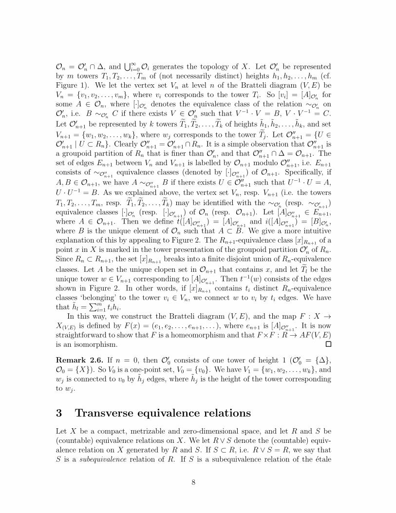
In [GPS2] the structure of a CEER, (R, T ) onX , is described. Figure 1 illustrateshow the structure looks like: X is decomposed into a finite number of m disjointclopen towers T1, T2, . . . , Tm, each of these consisting of finitely many disjoint clopensets. The equivalence classes of R are represented in Figure 1 as the family of setsconsisting of points lying on the same vertical line in each tower. (In the figure wehave marked the equivalence class [x1]R of a point x1 ∈ T1. We also show the graphpicture associated to the tower Tm of height three.)

Figure 1 also illustrates a concept that will play an important role in the sequel,namely a very special clopen partition of R, which we will refer to as a groupoidpartition. Let A and B be two (clopen) floors in the same tower, say the tower T1.There is a homeomorphism γ : A → B such that graph(γ) = {(x, γ(x)) | x ∈ A} ⊂R. Let O′ be the (finite) clopen partition of R consisting of the set of these graphsγ, and let O be the associated (finite) clopen partition of X (which we identify withthe diagonal ∆ = ∆X). So O = O′ ∩ ∆, which means that A ∈ O if A = B andγ : A → B is the identity map. The properties of O′ are as follows (where we defineU ·V for subsets U, V of R to be U ·V = {(x, z) | (x, y) ∈ U, (y, z) ∈ V for some y ∈X}):

(i) O′ is a finite clopen partition of R finer than {∆, R \∆}.

(ii) For all U ∈ O′, the maps r, s : U → X are homeomorphisms onto theirrespective images, and if U ⊂ R \∆, then r(U) ∩ s(U) = ∅.

(iii) For all U, V ∈ O′, we have U · V = ∅ or U · V ∈ O′. Also, U−1(= {(y, x) |(x, y) ∈ U}) is in O′ for every U in O′.

4

T1

A

B

✻γ

r

r

r

r

r

r

r

r

r

x1

■γ

T2

q q q

Tm

��

��

��

��

��

��

��

��

��

××× ××× ×××

×××

×××

×××

X

X

Tm

Tm

×××= Tm

Figure 1: Illustration of the groupoid partition of a CEER; R ⊂ X ×X

(iv) With O′(2) = {(U, V ) | U, V ∈ O′, U · V 6= ∅}, define (U, V ) ∈ O′(2) 7→ U · V ∈O′.

Then O′ has a principal groupoid structure with unit space equal to {U ∈ O′ | U ⊂∆} (which clearly may be identified with O). Hence the name groupoid partitionfor O′. (Note that if we think of U and V as maps, then U · V means first applyingthe map U and then the map V .)

Note that if we define the equivalence relation ∼O′ on O by A ∼O′ B if thereexists U ∈ O′ such that U−1 ·U = A, U ·U−1 = B, then the equivalence classes [·]O′

are exactly the towers in Figure 1. The heights of the various towers T1, T2, . . . , Tm

in Figure 1 are not necessarily distinct. All the groupoid partitions of R finer thanthe one shown in Figure 1 are obtained by vertically dividing the various towersT1, T2, . . . , Tm (by clopen sets) in an obvious way.

The proof of the following proposition can be found in [GPS2, Lemma 3.4, Corol-lary 3.5].

Proposition 2.2. Let (R, T ) be a CEER on X, and let V ′ and V be (finite) clopenpartitions of R and X, respectively. There exists a groupoid partition O′ of R whichis finer than V ′, and such that O = O′ ∩ ∆ is a clopen partition of X that is finerthan V.

Definition 2.3 (AF and AF-able (affable) equivalence relations). Let {(Rn, Tn)}∞n=0

be an ascending sequence of CEERs on X (compact, metrizable, zero-dimensional),that is, Rn ⊂ Rn+1 and Rn ∈ Tn+1 (i.e. Rn is open in Rn+1) for n = 0, 1, 2, . . . ,where we set R0 = ∆X(∼= X), T0 being the topology on X . Let (R, T ) be theinductive limit of {(Rn, Tn)} with the inductive limit topology T , i.e. R =

⋃∞

n=0Rn

5

and U ∈ T if U ∩ Rn ∈ Tn for any n. In particular, Rn is an open subset of Rfor all n. We say that (R, T ) is an AF-equivalence relation on X , and we use thenotation (R, T ) = lim

−→(Rn, Tn). We say that an equivalence relation S on X is AF-

able (affable) if it can be given a topology making it an AF-equivalence relation.(Note that this is the same as to say that S is orbit equivalent to an AF-equivalencerelation, cf. Definition 1.3.)

Remark 2.4. One can prove that (R, T ) is an AF-equivalence relation if and onlyif (R, T ) is the inductive limit of an ascending sequence {(Rn, Tn)}

∞n=0, where all the

(Rn, Tn) are etale and finite (i.e. the Rn-equivalence classes are finite) equivalencerelations, not necessarily CEERs, cf. [M]. This fact highlights the analogy betweenAF-equivalence relations in the topological setting with the so-called hyperfiniteequivalence relations in the Borel and measure-theoretic setting.

It can be shown that the condition that Rn is open in Rn+1 is superfluous whenRn and Rn+1 are CEERs (see the comment right after Definition 3.7 of [GPS2]).

We will assume some familiarity with the notion of a Bratteli diagram (cf. [GPS2]for details). We remind the reader of the notation we will use. Let (V,E) be aBratteli diagram, where V is the vertex set and E is the edge set, and where V ,respectively E, can be written as a countable disjoint union of finite non-empty sets:

V = V0 ∪ V1 ∪ V2 ∪ . . . and E = E1 ∪ E2 ∪ . . .

with the following property: an edge e in En connects a vertex v in Vn−1 to a vertexw in Vn. We write i(e) = v and t(e) = w, where we call i the source (or initial) mapand t the range (or terminal) map. So a Bratteli diagram has a natural grading,and we will say that Vn is the vertex set at level n. We require that i−1(v) 6= ∅ forall v ∈ V and t−1(v) 6= ∅ for all v ∈ V \V0. We also want our Bratteli diagram to bestandard, i.e. V0 = {v0} is a one-point set. In the sequel all our Bratteli diagramsare assumed to be standard, so we drop the term ‘standard’. Let

X(V,E) = {(e1, e2, . . . ) | en ∈ En, t(en) = i(en+1) for all n ∈ N}

be the path space associated to (V,E). Equipped with the relative topology fromthe product space

∏nEn, X(V,E) is compact, metrizable and zero-dimensional. We

denote the cofinality relation on (V,E) by AF (V,E), that is, two paths are equivalentif they agree from some level on. We now equip AF (V,E) with an AF-structure.Let n ∈ {0, 1, 2, . . .}. Then AFn(V,E) will denote the compact etale subequivalencerelation of AF (V,E) defined by the property of cofinality from level n on. Thatis, if x = (e1, e2, . . . , en, en+1, . . . ), y = (f1, f2, . . . , fn, fn+1, . . . ) is in X(V,E), then(x, y) ∈ AFn(V,E) if en+1 = fn+1, en+2 = fn+2, . . . , and AFn(V,E) is given therelative topology from X(V,E) × X(V,E), thus getting a CEER structure. ObviouslyAFn(V,E) ⊂ AFn+1(V,E), and we have AF (V,E) =

⋃∞

n=0AFn(V,E). We giveAF (V,E) the inductive limit topology, i.e. AF (V,E) = lim

−→AFn(V,E).

6

T1

r

r

r

r

r

r

r

r

r

r

r

r

r

r

r

r

r

r

T2

r

r

r

r

r

rx

q q q

Tm

r

r

r

r

r

r

r

r

r

s

s s q q q s

✓✓✓✓✓✓✓

w = Tl

v1qT1

v2qT2

vmqTm

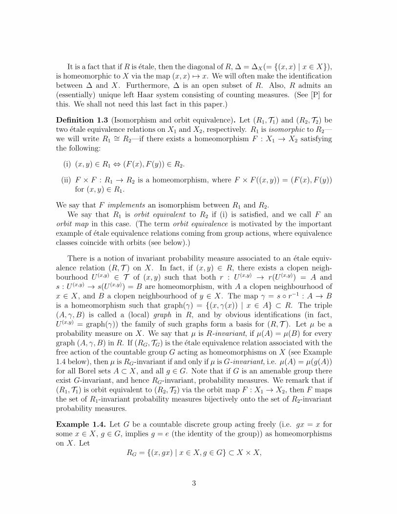
Figure 2: Illustration of the maps i, t : E → V

Let p = (e1, e2, . . . , en) be a finite path from level 0 to some level n, and let U(p)denote the cylinder set in X(V,E) defined by

U(p) = {x = (f1, f2, . . . ) ∈ X(V,E) | f1 = e1, f2 = e2, . . . , fn = en}.

Then U(p) is a clopen subset of X(V,E), and the collection of all cylinder sets isa clopen basis for X(V,E). Let p = (e1, e2, . . . , en) and q = (e′1, e

′2, . . . , e

′n) be two

finite paths from level 0 to the same level n, such that t(en) = t(e′n). Let U(p, q)denote the intersection of AFn(V,E) with the Cartesian product U(p)× U(q). Thecollection of sets of the form U(p, q) is a clopen basis for AF (V,E). From this itfollows immediately that a probability measure µ on X(V,E) is AF (V,E)-invariant(cf. Section 1) if and only if µ(U(p)) = µ(U(q)) for all such cylinder sets U(p) andU(q).

The following theorem is proved in [GPS2, Theorem 3.9]. However, we willexplain the salient feature of the proof, as this will be important for arguments laterin this paper.

Theorem 2.5. Let (R, T ) = lim−→

(Rn, Tn) be an AF-equivalence relation on X. There

exists a Bratteli diagram (V,E) such that (R, T ) is isomorphic to the AF-equivalencerelation AF (V,E) associated to (V,E). Furthermore, (V,E) is simple if and only if(R, T ) is minimal.

Proof sketch. For each n, choose a partition P ′n of Rn such that

⋃∞

n=0P′n generates

the topology T of R. (We assume that R0 equals ∆(= ∆X), the diagonal of X ,and we will freely identify X with ∆ whenever that is convenient.) Assume we haveinductively obtained a groupoid partition O′

n of Rn which is finer than both P ′n and

O′n−1 ∪ {Rn \Rn−1}, cf. Proposition 2.2. Obviously On+1 = O′

n+1 ∩∆ is finer than

7

On = O′n ∩ ∆, and

⋃∞

i=0Oi generates the topology of X . Let O′n be represented

by m towers T1, T2, . . . , Tm of (not necessarily distinct) heights h1, h2, . . . , hm (cf.Figure 1). We let the vertex set Vn at level n of the Bratteli diagram (V,E) beVn = {v1, v2, . . . , vm}, where vi corresponds to the tower Ti. So [vi] = [A]O′

nfor

some A ∈ On, where [·]O′

ndenotes the equivalence class of the relation ∼O′

non

O′n, i.e. B ∼O′

nC if there exists V ∈ O′

n such that V −1 · V = B, V · V −1 = C.

Let O′n+1 be represented by k towers T1, T2, . . . , Tk of heights h1, h2, . . . , hk, and set

Vn+1 = {w1, w2, . . . , wk}, where wj corresponds to the tower Tj . Let O′′n+1 = {U ∈

O′n+1 | U ⊂ Rn}. Clearly O′′

n+1 = O′n+1∩Rn. It is a simple observation that O′′

n+1 isa groupoid partition of Rn that is finer than O′

n, and that O′′n+1 ∩∆ = On+1. The

set of edges En+1 between Vn and Vn+1 is labelled by On+1 modulo O′′n+1, i.e. En+1

consists of ∼O′′

n+1equivalence classes (denoted by [·]O′′

n+1) of On+1. Specifically, if

A,B ∈ On+1, we have A ∼O′′

n+1B if there exists U ∈ O′′

n+1 such that U−1 · U = A,

U · U−1 = B. As we explained above, the vertex set Vn, resp. Vn+1 (i.e. the towers

T1, T2, . . . , Tm, resp. T1, T2, . . . , Tk) may be identified with the ∼O′

n(resp. ∼O′

n+1)

equivalence classes [·]O′

n(resp. [·]O′

n+1) of On (resp. On+1). Let [A]O′′

n+1∈ En+1,

where A ∈ On+1. Then we define t([A]O′′

n+1) = [A]O′

n+1and i([A]O′′

n+1) = [B]O′

n,

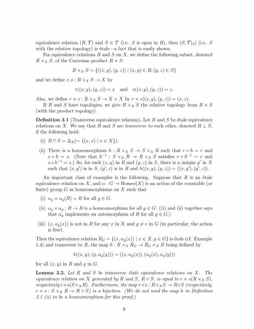
where B is the unique element of On such that A ⊂ B. We give a more intuitiveexplanation of this by appealing to Figure 2. The Rn+1-equivalence class [x]Rn+1 of apoint x in X is marked in the tower presentation of the groupoid partition O′

n of Rn.Since Rn ⊂ Rn+1, the set [x]Rn+1 breaks into a finite disjoint union of Rn-equivalence

classes. Let A be the unique clopen set in On+1 that contains x, and let Tl be theunique tower w ∈ Vn+1 corresponding to [A]O′

n+1. Then t−1(w) consists of the edges

shown in Figure 2. In other words, if [x]Rn+1 contains ti distinct Rn-equivalenceclasses ‘belonging’ to the tower vi ∈ Vn, we connect w to vi by ti edges. We havethat hl =

∑m

i=1 tihi.In this way, we construct the Bratteli diagram (V,E), and the map F : X →

X(V,E) is defined by F (x) = (e1, e2, . . . , en+1, . . . ), where en+1 is [A]O′′

n+1. It is now

straightforward to show that F is a homeomorphism and that F×F : R → AF (V,E)is an isomorphism.

Remark 2.6. If n = 0, then O′0 consists of one tower of height 1 (O′

0 = {∆},O0 = {X}). So V0 is a one-point set, V0 = {v0}. We have V1 = {w1, w2, . . . , wk}, andwj is connected to v0 by hj edges, where hj is the height of the tower correspondingto wj .

3 Transverse equivalence relations

Let X be a compact, metrizable and zero-dimensional space, and let R and S be(countable) equivalence relations on X . We let R∨S denote the (countable) equiv-alence relation on X generated by R and S. If S ⊂ R, i.e. R ∨ S = R, we say thatS is a subequivalence relation of R. If S is a subequivalence relation of the etale

8

equivalence relation (R, T ) and S ∈ T (i.e. S is open in R), then (S, T |S) (i.e. Swith the relative topology) is etale—a fact that is easily shown.

For equivalence relations R and S on X , we define the following subset, denotedR×X S, of the Cartesian product R× S:

R ×X S = {((x, y), (y, z)) | (x, y) ∈ R, (y, z) ∈ S}

and we define r, s : R×X S → X by

r((x, y), (y, z)) = x and s((x, y), (y, z)) = z.

Also, we define r × s : R ×X S → X ×X by r × s((x, y), (y, z)) = (x, z).If R and S have topologies, we give R ×X S the relative topology from R × S

(with the product topology).

Definition 3.1 (Transverse equivalence relation). Let R and S be etale equivalencerelations on X . We say that R and S are transverse to each other, denoted R ⊥ S,if the following hold:

(i) R ∩ S = ∆X(= {(x, x) | x ∈ X}).

(ii) There is a homeomorphism h : R ×X S → S ×X R such that r ◦ h = r ands ◦ h = s. (Note that h−1 : S ×X R → R ×X S satisfies r ◦ h−1 = r ands ◦ h−1 = s.) So, for each (x, y) in R and (y, z) in S, there is a unique y′ in Xsuch that (x, y′) is in S, (y′, z) is in R and h((x, y), (y, z)) = ((x, y′), (y′, z)).

An important class of examples is the following. Suppose that R is an etaleequivalence relation on X , and α : G → Homeo(X) is an action of the countable (orfinite) group G as homeomorphisms on X such that

(i) αg × αg(R) = R for all g ∈ G.

(ii) αg ×αg : R → R is a homeomorphism for all g ∈ G. ((i) and (ii) together saysthat αg implements an automorphism of R for all g ∈ G.)

(iii) (x, αg(x)) is not in R for any x in X and g 6= e in G (in particular, the actionis free).

Then the equivalence relationRG = {(x, αg(x)) | x ∈ X, g ∈ G} is etale (cf. Example1.4) and transverse to R, the map h : R×X RG → RG ×X R being defined by

h((x, y), (y, αg(y))) = ((x, αg(x)), (αg(x), αg(y)))

for all (x, y) in R and g in G.

Lemma 3.2. Let R and S be transverse etale equivalence relations on X. Theequivalence relation on X generated by R and S, R ∨ S, is equal to r × s(R×X S),respectively r×s(S×XR). Furthermore, the map r×s : R×XS → R∨S (respectively,r × s : S ×X R → R ∨ S) is a bijection. (We do not need the map h in Definition3.1 (ii) to be a homeomorphism for this proof.)

9

Proof. We consider the map r × s : R ×X S → R ∨ S (it being obvious that thearguments we give apply similarly to the map r × s : S ×X R → R ∨ S, since byDefinition 3.1 (ii), r× s(R×X S) = r× s(S×X R)). Clearly r× s(R×X S) ⊂ R∨S.If (x, y) ∈ R, then ((x, y), (y, y)) ∈ R ×X S, and so (x, y) ∈ r × s(R ×X S). HenceR ⊂ r × s(R ×X S). Likewise we show that S ⊂ r × s(R ×X S). If (x, z) equalsr×s((x, y), (y, z)) = r×s((x, y′), (y′, z)), then (x, y), (x, y′) are in R, and so (y, y′) ∈R. Likewise, (y, z), (y′, z) are in S, and so (y, y′) ∈ S. Hence y = y′, and so the mapr× s is injective. The proof will be completed by showing that K = r× s(R×X S)is an equivalence relation on X .

Clearly, K is reflexive. To prove symmetry, assume (x, z) ∈ K. There existsy ∈ X such that (x, y) ∈ R, (y, z) ∈ S, and so ((z, y), (y, x)) ∈ S ×X R. Sincer × s(S ×X R) = r × s(R×X S), we get that (z, x) ∈ K. Hence K is symmetric.

To prove transitivity, assume (x, z), (z, w) ∈ K. We must show that (x, w) ∈ K.There exists y, y′ ∈ X such that ((x, y), (y, z)), ((z, y′), (y′, w)) ∈ R ×X S. Thisimplies that ((y, z), (z, y′)) ∈ S ×X R. Since the map h : R ×X S → S ×X R isa bijection, there exists y′′ ∈ X such that ((y, y′′), (y′′, y′)) ∈ R ×X S. We thusget that (y′, w), (y′′, y′) ∈ S, which implies that (y′′, w) ∈ S. Also, we have that(x, y), (y, y′′) ∈ R, which implies that (x, y′′) ∈ R. Hence ((x, y′′), (y′′, w)) ∈ R×X S,which implies that (x, w) ∈ r × s(R×X S) = K, which proves transitivity.

Proposition 3.3. Let (R, T ) and (S, T ) be two etale equivalence relations on Xwhich are transverse to each other. By the bijective map (cf. Lemma 3.2) r × s :R ×X S → R ∨ S, which sends ((x, y), (y, z)) ∈ R ×X S to (x, z), we transfer thetopology on R ×X S(⊂ R × S) to R ∨ S. With this topology, denoted W, R ∨ Sis an etale equivalence relation on X. In particular, if R and S are CEERs, then(R∨S,W) is a CEER. Furthermore, W is the unique etale topology on R∨S, which

extends T on R and T on S, i.e. the relative topologies on R and S are T and T ,respectively. Also R and S are both open subsets of R ∨ S.

Proof. It is easily seen that R×X S is a closed subset of R× S, and so the relativetopology on R×X S, and consequently W, is locally compact and metrizable. If Rand S are CEERs, then clearly R ×X S is compact. Now R (resp. S) is the imageunder r × s of

R×X ∆ = {((x, y), (y, y)) | (x, y) ∈ R}

(resp. ∆×X S = {((x, x), (x, y)) | (x, y) ∈ S}),

where ∆ = ∆X is the diagonal of X ×X . Now R×X ∆ (resp. ∆×X S) is clopen inR×X S, since ∆ is clopen in R (resp. S), and so we get that R (resp. S) is clopenin R ∨ S.

We now show the etale condition for R ∨ S. Let (x, z) ∈ R∨ S, and let y be theunique point in X such that ((x, y), (y, z)) ∈ R ×X S. A local basis at (x, z) is the

family of composition of graphs in T and T (cf. Section 1)

(U , γ, V ) ◦ (U, γ, V ) = (U ∩ γ−1(V ∩ U), γ ◦ γ, γ(V ∩ U)),

10

where (U, γ, V ) ∈ T , (U , γ, V ) ∈ T , and x ∈ U , y ∈ V ∩ U , z ∈ V , such that

y = γ(x), z = γ(y). In fact, we may assume that U = V , and so a local basis at(x, z) is the family of graphs

{(U, γ ◦ γ, V )

∣∣∣∣x ∈ U, z ∈ V, U and V open in X,

V = γ ◦ γ(U), graph(γ) ⊂ R, graph(γ) ⊂ S

}.

Clearly each (U, γ ◦ γ, V ) is an etale open neighbourhood of (x, z) in W. We needto show that the product of composable pairs in R ∨ S is continuous, and also thatthe inverse map on R ∨ S is continuous. If we assume this has been established,it follows easily that any etale topology E on R ∨ S that extends T on R and Ton S has to be equal to W. In fact, since (x, y) · (y, z) = (x, z), where (x, y) ∈ R,(y, z) ∈ S, it is easy to show that the graphs (U, γ ◦ γ, V ) considered above is alsoa local basis for E at (x, z). Thus, W is contained in E . The other inclusion followseasily from the etaleness of E .

To prove that the map (x, z) 7→ (x, z)−1 = (z, x) is continuous (and hencea homeomorphism) on R ∨ S, let (xn, zn) → (x, z). This means that there ex-ist (unique) yn, y ∈ X such that ((xn, yn), (yn, zn)) → ((x, y), (y, z)) in R ×X S.This implies that ((zn, yn), (yn, xn)) → ((z, y), (y, x)) in S ×X R. Applying themap h of Definition 3.1 (ii), we conclude that there exist y′n, y

′ ∈ X such that((zn, y

′n), (y

′n, xn)) → ((z, y′), (y′, x)) in R ×X S. This means that (zn, xn) → (z, x)

in R ∨ S, and we are done.To prove that the product of composable pairs in (R ∨ S)× (R ∨ S) is continu-

ous, let ((xn, yn), (yn, zn)) → ((x, y), (y, z)) in (R ∨ S)× (R ∨ S). We want to showthat (xn, zn) → (x, z) in R ∨ S. There exist (unique) y′n, y

′′n, y

′, y′′ ∈ X such that((xn, y

′n), (y

′n, yn)) → ((x, y′), (y′, y)) and ((yn, y

′′n), (y

′′n, zn)) → ((y, y′′), (y′′, z)) in

R×X S. This implies that ((y′n, yn), (yn, y′′n)) → ((y′, y), (y, y′′)) in S×XR. Using the

map h of Definition 3.1 (ii), there exist y′′′n , y′′′ ∈ X such that ((y′n, y

′′′n ), (y

′′′n , y

′′n)) →

((y′, y′′′), (y′′′, y′′)) in R ×X S. So we have altogether (xn, y′n) → (x, y′), (y′n, y

′′′n ) →

(y′, y′′′) in R, (y′′′n , y′′n) → (y′′′, y′′), (y′′n, zn) → (y′′, z) in S. This implies that

(xn, y′′′n ) → (x, y′′′) in R, and (y′′′n , zn) → (y′′′, z) in S. Hence ((xn, y

′′′n ), (y

′′′n , zn)) →

((x, y′′′), (y′′′, z)) in R×X S, and so (xn, zn) → (x, z) in R ∨ S.

Henceforth, whenever (R, T ) and (S, T ) are two transverse equivalence relationson X , we will give R ∨ S the etale topology W described in Proposition 3.3.

We want to prove that if R is an AF-equivalence relation on X , and S is aCEER on X such that R ⊥ S (i.e. R and S are transverse), then R ∨ S is againAF. Furthermore, we will give an explicit description of the relation between theBratteli diagram models for R ∨ S and R, respectively. This will be important forthe proof of the absorption theorem in the next section. We shall need the followingtwo lemmas.

Lemma 3.4. Let (R, T ) and (S, T ) be two transverse CEERs on X. Then thefollowing hold:

11

(i) (x, y) ∈ R ⇒ #([x]S) = #([y]S). (In fact, R does not have to be a CEER for(i) to hold.)

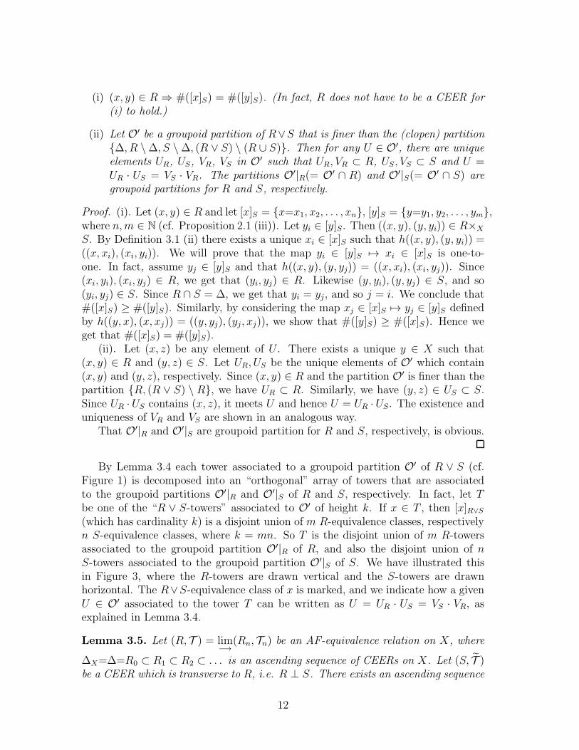
(ii) Let O′ be a groupoid partition of R∨S that is finer than the (clopen) partition{∆, R \∆, S \∆, (R ∨ S) \ (R ∪ S)}. Then for any U ∈ O′, there are uniqueelements UR, US, VR, VS in O′ such that UR, VR ⊂ R, US, VS ⊂ S and U =UR · US = VS · VR. The partitions O′|R(= O′ ∩ R) and O′|S(= O′ ∩ S) aregroupoid partitions for R and S, respectively.

Proof. (i). Let (x, y) ∈ R and let [x]S = {x=x1, x2, . . . , xn}, [y]S = {y=y1, y2, . . . , ym},where n,m ∈ N (cf. Proposition 2.1 (iii)). Let yi ∈ [y]S. Then ((x, y), (y, yi)) ∈ R×X

S. By Definition 3.1 (ii) there exists a unique xi ∈ [x]S such that h((x, y), (y, yi)) =((x, xi), (xi, yi)). We will prove that the map yi ∈ [y]S 7→ xi ∈ [x]S is one-to-one. In fact, assume yj ∈ [y]S and that h((x, y), (y, yj)) = ((x, xi), (xi, yj)). Since(xi, yi), (xi, yj) ∈ R, we get that (yi, yj) ∈ R. Likewise (y, yi), (y, yj) ∈ S, and so(yi, yj) ∈ S. Since R ∩ S = ∆, we get that yi = yj, and so j = i. We conclude that#([x]S) ≥ #([y]S). Similarly, by considering the map xj ∈ [x]S 7→ yj ∈ [y]S definedby h((y, x), (x, xj)) = ((y, yj), (yj, xj)), we show that #([y]S) ≥ #([x]S). Hence weget that #([x]S) = #([y]S).

(ii). Let (x, z) be any element of U . There exists a unique y ∈ X such that(x, y) ∈ R and (y, z) ∈ S. Let UR, US be the unique elements of O′ which contain(x, y) and (y, z), respectively. Since (x, y) ∈ R and the partition O′ is finer than thepartition {R, (R ∨ S) \ R}, we have UR ⊂ R. Similarly, we have (y, z) ∈ US ⊂ S.Since UR ·US contains (x, z), it meets U and hence U = UR ·US. The existence anduniqueness of VR and VS are shown in an analogous way.

That O′|R and O′|S are groupoid partition for R and S, respectively, is obvious.

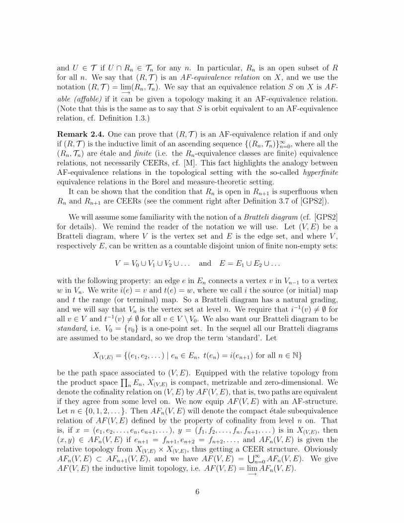
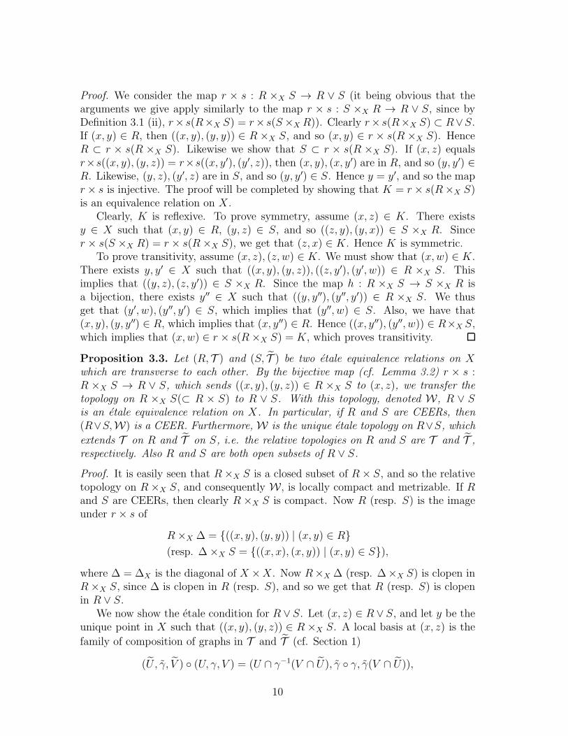
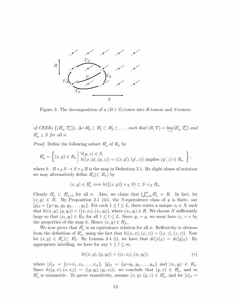
By Lemma 3.4 each tower associated to a groupoid partition O′ of R ∨ S (cf.Figure 1) is decomposed into an “orthogonal” array of towers that are associatedto the groupoid partitions O′|R and O′|S of R and S, respectively. In fact, let Tbe one of the “R ∨ S-towers” associated to O′ of height k. If x ∈ T , then [x]R∨S

(which has cardinality k) is a disjoint union of m R-equivalence classes, respectivelyn S-equivalence classes, where k = mn. So T is the disjoint union of m R-towersassociated to the groupoid partition O′|R of R, and also the disjoint union of nS-towers associated to the groupoid partition O′|S of S. We have illustrated thisin Figure 3, where the R-towers are drawn vertical and the S-towers are drawnhorizontal. The R∨S-equivalence class of x is marked, and we indicate how a givenU ∈ O′ associated to the tower T can be written as U = UR · US = VS · VR, asexplained in Lemma 3.4.

Lemma 3.5. Let (R, T ) = lim−→

(Rn, Tn) be an AF-equivalence relation on X, where

∆X=∆=R0 ⊂ R1 ⊂ R2 ⊂ . . . is an ascending sequence of CEERs on X. Let (S, T )be a CEER which is transverse to R, i.e. R ⊥ S. There exists an ascending sequence

12

✑✑✑

✑✑✑

✑✑✑

✑✑✑

✑✑✑

✑✑✑

✑✑✑

✑✑✑

✑✑✑

✑✑✑

✑✑✑

✑✑✑

✑✑✑

✑✑✑

✑✑✑

r r r r r

r r r r r

r r r r r

✻

❄

R

✲✛S

✒U

❘

US

✿VS

✒

UR

■VR

Figure 3: The decomposition of a (R ∨ S)-tower into R-towers and S-towers

of CEERs {(R′n, T

′n)}, ∆=R′

0 ⊂ R′1 ⊂ R′

2 ⊂ . . . , such that (R, T ) = lim−→

(R′

n, T′

n) and

R′n ⊥ S for all n.

Proof. Define the following subset R′n of Rn by

R′

n =

{(x, y) ∈ Rn

∣∣∣∣∀(y, z) ∈ S,h((x, y), (y, z)) = ((x, y′), (y′, z)) implies (y′, z) ∈ Rn

},

where h : R×X S → S×XR is the map in Definition 3.1. By slight abuse of notationwe may alternatively define R′

n(⊂ Rn) by

(x, y) ∈ R′

n ⇐⇒ h({(x, y)} ×X S) ⊂ S ×X Rn.

Clearly R′n ⊂ R′

n+1 for all n. Also, we claim that⋃

∞

n=0R′n = R. In fact, let

(x, y) ∈ R. By Proposition 2.1 (iii), the S-equivalence class of y is finite, say[y]S = {y=y1, y2, y3, . . . , yL}. For each 1 ≤ l ≤ L, there exists a unique xl ∈ X suchthat h((x, y), (y, yl)) = ((x, xl), (xl, yl)), where (xl, yl) ∈ R. We choose N sufficientlylarge so that (xl, yl) ∈ RN for all 1 ≤ l ≤ L. Since y1 = y, we must have x1 = x bythe properties of the map h. Hence (x, y) ∈ R′

N .We now prove that R′

n is an equivalence relation for all n. Reflexivity is obviousfrom the definition of R′

n, using the fact that h((x, x), (x, z)) = ((x, z), (z, z)). Nowlet (x, y) ∈ R′

n(⊂ R). By Lemma 3.4 (i), we have that #([x]S) = #([y]S). Byappropriate labelling, we have for any 1 ≤ l ≤ m,

h((x, y), (y, yl)) = ((x, xl), (xl, yl)), (∗)

where [x]S = {x=x1, x2, . . . , xm}, [y]S = {y=y1, y2, . . . , ym} and (xl, yl) ∈ Rn.Since h((y, x), (x, xl)) = ((y, yl), (yl, xl)), we conclude that (y, x) ∈ R′

n, and soR′

n is symmetric. To prove transitivity, assume (x, y), (y, z) ∈ R′n, and let [x]S =

13

{x=x1, x2, . . . , xm}, [y]S = {y=y1, . . . , ym}, [z]S = {z=z1, z2, . . . , zm}. The labellingis done as explained above (cf. (∗)), so that (xl, yl), (yl, zl) ∈ Rn for 1 ≤ l ≤ m.Since (xl, zl) ∈ Rn, we get that h((x, z), (z, zl)) = ((x, xl), (xl, zl)) for all 1 ≤ l ≤ m.This implies that (x, z) ∈ R′

n, thus finishing the proof that R′n is an equivalence

relation.Note that we can use (∗) to deduce that the map h (or rather, its restriction), h :

R′n×X S → S×X R′

n, is a bijection. In fact, let l be fixed, 1 ≤ l ≤ m. We must showthat (xl, yl) in (∗) lies in R′

n. We have that h((yl, xl), (xl, xj)) = ((yl, yj), (yj, xj)) forall 1 ≤ j ≤ m. Since (yj, xj) ∈ Rn for 1 ≤ j ≤ m, we conclude that (yl, xl), andhence (xl, yl), is in R′

n.Obviously we have R′

n ∩ S = ∆. So to finish the proof, it is sufficient to showthat R′

n is a clopen subset of Rn. We claim that

R′

n ×X S = (Rn ×X S) ∩ h−1(S ×X Rn). (∗∗)

In fact, it is clear that the set on the left hand side of (∗∗) is contained in the set onthe right hand side of (∗∗). Conversely, let ((x, y), (y, z)) ∈ (Rn×XS)∩h

−1(S×XRn).Then (x, y) ∈ Rn, and h((x, y), (y, z)) = ((x, y′), (y′, z)) implies (y′, z) ∈ Rn. So(x, y) ∈ R′

n, proving the other inclusion of (∗∗).Now Rn ×X S and S ×X Rn are easily seen to be closed subsets of the Cartesian

products Rn × S and S ×Rn, respectively (cf. Proposition 2.1 (i)). Hence they arecompact and, a fortiori, closed subsets of R ×X S and S ×X R, respectively. SinceRn is open in R, it follows easily that Rn ×X S and S ×X Rn are open subsets ofR×X S and S×X R, respectively. From (∗∗) we conclude that R′

n×X S is a compactand open subset of R ×X S. Now R′

n = π1(R′n ×X S), where π1 : R × S → R is

the projection map. Since π1 is a continuous and open map, we conclude that R′n is

compact and open in R, and hence in Rn. This completes the proof.

Proposition 3.6. Let (R, T ) = lim−→

(Rn, Tn) be an AF-equivalence relation on X,

and let S be a CEER on X such that R ⊥ S, i.e. R and S are transverse to eachother. Then R ∨ S is an AF-equivalence relation.

Furthermore, there exist Bratteli diagrams (V,E) and (V ′, E ′) such that

R ∼= AF (V,E), R′ = R ∨ S ∼= AF (V ′, E ′)

and so that t : E1 → V1 is injective and S ∼= AF1(V′, E ′). Moreover, there are

surjective maps (respecting gradings) qV : V → V ′ and qE : E → E ′ such that

(i) i(qE(e)) = qV (i(e)), t(qE(e)) = qV (t(e)) for e in E.

(ii) For each v in V , qE : i−1({v}) → i−1({qV (v)}) is a bijection.

(iii) For each v ∈ Vn and n ≥ 2, qE : t−1({v}) → t−1({qV (v)}) is a bijection.

The map H : X(V,E) → X(V ′,E′) defined by

x = (e1, e2, e3, . . . ) 7→ H(x) = (qE(e1), qE(e2), qE(e3), . . . )

14

is a homeomorphism, and H implements an embedding of AF (V,E) into AF (V ′, E ′)whose image is transverse to AF1(V

′, E ′) ∼= S. Moreover, we have

AF1(V′, E ′) ∨ (H ×H)(AF (V,E)) ∼= AF (V ′, E ′).

(Recall the notation and terminology we introduced in Section 2. In particular,V = V0∪V1∪V2∪ . . . , E = E1∪E2∪ . . . , V ′ = V ′

0∪V ′1∪V ′

2∪ . . . , E ′ = E ′1∪E ′

2∪ . . . .)

Proof. By Lemma 3.5, we may assume that Rn ⊥ S for all n. Now let (∆X =)∆ =R0 = R1 ⊂ R2 ⊂ R3 ⊂ . . . and

∆=R′

0 ⊂ R′

1=R1 ∨ S ⊂ R′

2=R2 ∨ S ⊂ R′

3=R3 ∨ S ⊂ · · · ⊂ R′ = R ∨ S =∞⋃

n=0

R′

n.

Applying Proposition 3.3 we can conclude that R∨S is an AF-equivalence relation.Now let P ′

n be a groupoid partition of R′n = Rn ∨ S which is finer than both

P ′n−1 ∪ {R′

n \R′n−1} and {∆, Rn \∆, S \∆, R′

n \ (Rn ∪ S)}, where we set P ′0 = {∆}.

We require that⋃

∞

n=0P′n generates the topology of R ∨ S. (This can be achieved

by successive applications of Proposition 2.2.) By Lemma 3.4 we get that O′n =

P ′n|Rn

(= P ′n ∩ Rn) is a groupoid partition of Rn for n ≥ 0, such that O′

n is finerthan both O′

n−1 ∪ {Rn \ Rn−1} and {∆, Rn \∆}. Furthermore,⋃

∞

n=0O′n generates

the topology of R. Similarly, Q′n = P ′

n|S(= P ′n ∩ S) is a groupoid partition of S

for n ≥ 1, such that Q′n is finer than both Q′

n−1 and {∆, S \ ∆}, and⋃

∞

n=0Q′n

generates the topology of S. (We set Q′0 = {∆}.) By Lemma 3.4, every U ∈ P ′

n

can be uniquely written as U = UR ·US , where UR ∈ O′n and US ∈ Q′

n, and we maysuggestively write P ′

n = O′n · Q

′n. For each n ≥ 0 we have that

(P ′

n ∩∆ =)P ′

n|∆ = O′

n|∆ = Q′

n|∆ = Pn

is a clopen partition of X , with

∆ = P0 ≺ P1 ≺ P2 ≺ . . .

and⋃

∞

n=0Pn being a basis for X .Combining all this—following the description given in the proof sketch of The-

orem 2.5— we construct the Bratteli diagrams (V ′, E ′) and (V,E), so that R′ =R ∨ S ∼= AF (V ′, E ′) and R ∼= AF (V,E), respectively, and such that the conditionsstated in the proposition are satisfied. For brevity we will omit some of the details,which are routine verifications, and focus on the main ingredients of the proof. (Wewill use the same notation that we used in the proof sketch of Theorem 2.5.)

First we observe that S ∼= AF1(V′, E ′). In fact, since P ′

0 = Q′0 = {∆}, and

P ′1 = Q′

1 is a groupoid partition of R′1 = ∆ ∨ S = S, the edge set E ′

1 is relatedin an obvious way to the towers {T1, T2, . . . , Tm} associated to Q′

1 (cf. Figures1 & 2 and Remark 2.6). The towers associated to Q′

n, n > 1, are obtained bysubdividing (vertically) the towers {T1, T2, . . . , Tm}, and from this it is easily seen

15

that S is isomorphic to AF1(V′, E ′). Since R0 = R1 = {∆}, and O′

0 = {∆},O′

1 = O′1|∆ = P1, we deduce that t : E1 → V1 is injective and that the obviously

defined maps, qV : V0 → V ′0 , qV : V1 → V ′

1 , qE : E1 → E ′1, satisfy condition (i) for

e ∈ E1, and (ii) for v ∈ V0. (For instance, if e ∈ E1 corresponds to A ∈ P1, thenit is mapped to e′ ∈ E ′

1, which corresponds to the “floor” A, that lies in one of thetowers {T1, T2, . . . , Tm}.)

Let n ≥ 1. Assume that we have defined qV : Vi → V ′i , i = 0, 1, . . . , n, and

qE : Ej → E ′j , j = 1, 2, . . . , n, such that (i) is true for e ∈ Ej , j = 1, 2, . . . , n, and

(ii) is true for v ∈ Vi, i = 0, 1, . . . , n − 1. Assume also that H((e1, e2, . . . , en)) =(qE(e1), qE(e2), . . . , qE(en)) is a bijection between finite paths of length n from thetop vertices of (V,E) and (V ′, E ′), respectively.

We now define qE : En+1 → E ′n+1. Let e = [A]O′′

n+1∈ En+1 for some A ∈

Pn+1(= P ′n+1|∆ = O′

n+1|∆), where O′′n+1 = {U ∈ O′

n+1 | U ⊂ Rn}. We defineqE(e) = [A]P ′′

n+1∈ E ′

n+1, where P′′n+1 = {W ∈ P ′

n+1 | W ⊂ R′n}. Since O′′

n+1 ⊂ P ′′n+1,

we get that qE : En+1 → E ′n+1 is well-defined and surjective. We define the map

qV : Vn+1 → V ′n+1 by qV (v) = [B]P ′

n+1∈ V ′

n+1, where v = [B]O′

n+1∈ Vn+1 for some

B ∈ Pn+1. Since O′n+1 ⊂ P ′

n+1, we get that the map qV is well-defined and surjective.It is easy to see that (i) is satisfied for all e ∈ En+1.

We show that the maps defined in (ii) and (iii) are surjective. Let v = [B]O′

n∈ Vn,

where B ∈ Pn (resp. w = [B]O′

n+1∈ Vn+1, where B ∈ Pn+1). So qV (v) = [B]P ′

n∈ V ′

n

(resp. qV (w) = [B]P ′

n+1∈ V ′

n+1). Let e′ = [A]P ′′

n+1∈ i−1({qV (v)}) ⊂ E ′

n+1, where

A ∈ Pn+1 (resp. f ′ = [A]P ′′

n+1∈ t−1({qV (w)}) ⊂ E ′

n+1, where A ∈ Pn+1). This

means that A ∼P ′′

nA′ ⊂ B, for some A′ ∈ Pn+1 (resp. A ∼P ′

n+1B, or, equivalently,

[A]P ′

n+1= [B]P ′

n+1). Let e = [A′]O′′

n+1∈ En+1 (resp. f = [A]O′′

n+1∈ En+1). Then

clearly i(e) = v and qE(e) = e′, proving that qE : i−1({v}) → i−1({qV (v)}) issurjective. Clearly qE(f) = f ′. Also, since n+1 ≥ 2, we have that P ′′

n+1|R′

1≻ Q′

1(=

P ′1 = P ′′

1 ), and so we may choose A such that A and B are contained in the same

set C ∈ P1. This fact, together with A ∼P ′

n+1B, implies that A ∼O′

n+1B. In fact,

if U = UR · US ∈ P ′n+1 such that U−1 · U = A, U · U−1 = B, with UR ∈ O′

n+1,

US ∈ Q′n+1, then U = UR, since US must be the identity map on B. Hence we get

that [A]O′

n+1= [B]O′

n+1= w, and so we have proved that the map qE : t−1({w}) →

t−1({qV (w)}) is surjective.We prove that (ii) holds for v ∈ Vn. Since qE : i−1({v}) → i−1({qV (v)}) is

surjective, we need to prove injectivity. So let e1, e2 ∈ i−1({v}), and assume qE(e1) =qE(e2). We must show that e1 = e2. Now e1 = [A]O′′

n+1, e2 = [B]O′′

n+1for some

A,B ∈ Pn+1. Since qE(e1) = qE(e2), we have that [A]P ′′

n+1= [B]P ′′

n+1. Hence there

exists U ∈ P ′n+1 such that U−1 · U = A, U · U−1 = B, and U ⊂ Rn ∨ S = R′

n.Since e1, e2 ∈ i−1({v}), we have that A ⊂ A1 ∈ Pn, B ⊂ B1 ∈ Pn, such that[A1]O′

n= [B1]O′

n; that is, there exists U1 ∈ O′

n ⊂ P ′n, such that U−1

1 · U1 = A1,U1 · U

−11 = B1. Since P ′

n+1|R′

nis finer than P ′

n, we must have U ⊂ U1(⊂ Rn). Thismeans that U ∈ O′′

n+1, and so e1 = [A]O′′

n+1= [B]O′′

n+1= e2.

16

(V,E)r

r r r r r

✟✟✟✟✟✟✟✟✟✟

��

��

�

❅❅❅❅❅

❍❍❍❍❍❍❍❍❍❍

︸ ︷︷ ︸(W,F )

︸ ︷︷ ︸(W,F )

︸ ︷︷ ︸(W,F )

︸ ︷︷ ︸(W , F )

︸ ︷︷ ︸(W , F )

(V ′, E ′)r

r r

✡✡

✡✡✡

❏❏❏❏❏

❏❏❏❏❏

︸ ︷︷ ︸(W,F )

︸ ︷︷ ︸(W , F )

Figure 4: Illustrating the content of Proposition 3.6

In a similar way we prove that (iii) holds. In fact, let e1, e2 ∈ t−1({v}), v ∈Vn+1, such that qE(e1) = qE(e2). We must show that e1 = e2. Again we writee1 = [A]O′′

n+1, e2 = [B]O′′

n+1for some A,B ∈ Pn+1. Since e1, e2 ∈ t−1({v}), we have

[A]O′

n+1= [B]O′

n+1, that is, there exists U1 ∈ O′

n+1 ⊂ P ′n+1 such that U−1

1 · U1 = A,

U1 ·U−11 = B. Since qE(e1) = qE(e2), we have [A]P ′′

n+1= [B]P ′′

n+1, that is, there exists

U ∈ P ′n+1 such that U−1 ·U = A, U ·U−1 = B, and U ⊂ Rn ∨S = R′

n. This impliesthat U = U1. Since U1 ⊂ Rn+1, U ⊂ Rn ∨ S and S ∩ Rn+1 = ∆, we must haveU1 ⊂ Rn. Hence U1 ∈ O′′

n+1, and so e1 = e2.It is now straightforward to verify that H : X(V,E) → X(V ′,E′) is a homeo-

morphism that implements an isomorphism between AF (V,E) and its image H ×H(AF (V,E)) in AF (V ′, E ′). The last assertion of the proposition is now routinelyverified.

Remark 3.7. It is helpful to illustrate by a figure what Proposition 3.6 says, andwhich at the same time gives the heuristics of the proof. Furthermore, the illustrationwill be useful for easier comprehending the proof of the main theorem in the nextsection. In Figure 4 we have drawn the diagrams of (V,E) and (V ′, E ′). The replicate

diagrams (W,F ) (resp. (W , F )) are also drawn, and S, the CEER transverse toR = AF (V,E), as well as the maps qV and qE , should be obvious from the figure.One sees that what is going on is a “glueing” process in the sense that distinctR-equivalence classes are “glued” together by S to form R′-equivalence classes.

17

4 The absorption theorem

Definition 4.1 (R-etale and R-thin sets). Let (R, T ) be an etale equivalence rela-tion on the compact, metrizable and zero-dimensional space X . Let Y be a closedsubset of X . We say that Y is R-etale if the restriction R ∩ (Y × Y ) of R to Y ,denoted by R|Y , is an etale equivalence relation in the relative topology.

We say that Y is R-thin if µ(Y ) = 0 for all R-invariant probability measures µ(cf. Section 1).

Remark 4.2. It can be proved (cf. Theorem 3.11 of [GPS2]) that if (R, T ) is an AF-equivalence relation and Y is R-etale, then R|Y is an AF-equivalence relation on Y .Furthermore, there exist a Bratteli diagram (V,E) and a Bratteli subdiagram (W,F )such that R ∼= AF (V,E), R|Y ∼= AF (W,F ). (By a Bratteli subdiagram (W,F ) of(V,E) we mean that F is a subset of E such that i(F ) = {v0}∪ t(F ), that is, (W,F )is a Bratteli diagram, where W = i(F ) and W0 = V0. We say that F induces an(edge) subdiagram of (V,E). Observe that, in general, if (W,F ) is a subdiagram of(V,E), then R|Y ∼= AF (W,F ), where R = AF (V,E) and Y = X(W,F ).)

We state a result from [GPS2] that will be crucial in proving the absorptiontheorem.

Theorem 4.3 (Lemma 4.15 of [GPS2]). Let (R1, T1) and (R2, T2) be two minimalAF-equivalence relations on the Cantor sets X1 and X2, respectively. Let Yi be aclosed Ri-etale and Ri-thin subset of Xi, i = 1, 2. Assume

(i) R1∼= R2.

(ii) There exists a homeomorphism α : Y1 → Y2 which implements an isomorphismbetween R1|Y1 and R2|Y2.

Then there exists a homeomorphism α : X1 → X2 which implements an isomorphismbetween R1 and R2, such that α|Y1 = α, i.e. α is an extension of α.

The following lemma is a technical result—easily proved—that we shall need forthe proof of the absorption theorem. In the sequel we will use the term “micro-scoping” (of a Bratteli diagram) in the restricted sense called “symbol splitting” in[GPS1, Section 3]. (Microscoping is a converse operation to that of “telescoping”.)

Lemma 4.4. Let (R, T ) be a minimal AF-equivalence relation on the Cantor setX. Let {an}

∞n=1 and {bn}

∞n=1 be sequences of natural numbers. Then there exists a

(simple) Bratteli diagram (V,E) such that R ∼= AF (V,E), and for each n ≥ 1

(i) #(Vn) ≥ an.

(ii) For all v ∈ Vn−1 and all w ∈ Vn, #({e ∈ En|i(e)=v, t(e)=w}) ≥ bn.

18

Proof. Let R ∼= AF (W,F ) for some (simple) Bratteli diagram (W,F ). By a finitenumber of telescopings and microscopings of the diagram (W,F ), we get (V,E) withthe desired properties (cf. [GPS1, Section 3]).

Remark 4.5. We make the general remark that telescoping or microscoping a Brat-teli diagram do not alter any of the essential properties attached to the diagram,like the associated path space and the AF-equivalence relation. In fact, there is anatural map between the path spaces of the original and the new Bratteli diagramswhich implements an isomorphism between the AF-equivalence relations associatedto the two diagrams. However, the versatility that these operations (i.e. telescop-ings and microscopings) give us in changing a given Bratteli diagram into one whichis more suitable for our purpose—like having enough “room” to admit appropriatesubdiagrams—is very helpful. This will be utilized extensively in the proof of theabsorption theorem. Note that a subdiagram (W,F ) of a Bratteli diagram (V,E)is being telescoped or microscoped (in an obvious way) simultaneously as theseoperations are applied to (V,E). For this reason we will sometimes, when it is con-venient, retain the old notation for the new diagrams, and this should not cause anyconfusion.

We can now state and prove the main result of this paper.

Theorem 4.6 (The absorption theorem). Let R = (R, T ) be a minimal AF-equivalencerelation on the Cantor set X, and let Y be a closed R-etale and R-thin subset of X.Let K = (K,S) be a compact etale equivalence relation on Y . Assume K ⊥ R|Y ,i.e. K is transverse to R|Y .

Then there is a homeomorphism h : X → X such that

(i) h×h(R∨K) = R, where R∨K is the equivalence relation on X generated byR and K. In other words, R ∨K is orbit equivalent to R, and, in particular,R ∨K is affable.

(ii) h(Y ) is R-etale and R-thin.

(iii) h|Y × h|Y : (R|Y ) ∨K → R|h(Y ) is a homeomorphism.

Proof. Roughly speaking, the idea of the proof is to define an (open) AF-subequivalencerelation R of R, thereby setting the stage for applying Theorem 4.3 (with R1 = R2 =R), and in the process “absorbing” Y (and thereby K) so that R∨K becomes R. Todefine R we will manipulate Bratteli diagrams, applying Lemma 4.4 together withProposition 3.6. The proof is rather technical, and to facilitate the understandingand get the main idea of the proof it will be helpful to have a very special, buttelling, example in mind. We refer to Remark 4.7 for details on this.

Let (W,F ) and (W ′, F ′) be two (fixed) Bratteli diagrams such that

R|Y ∼= AF (W,F ), R|Y ∨K ∼= AF (W ′, F ′)

19

and letqW : W → W ′, qF : F → F ′, H : X(W,F ) → X(W ′,F ′)

be maps satisfying the conditions of Proposition 3.6. By Theorem 3.11 of [GPS2]

there exist a (simple) Bratteli diagram (V,E) and a subdiagram (W , F ) such thatwe may assume from the start that X = X(V,E), Y = X(fW, eF ), R = AF (V,E),

R|Y = AF (W , F ). By a finite number of telescopings and microscopings applied to

(V,E), and hence to (W , F ), we may assume that for all n ≥ 1, #(Wn) ≤12#(Vn),

and for v0 ∈ V0 = W0, w ∈ Wn,

#({paths in X(fW, eF ) from v0 to w}) ≤1

2#({paths in X(V,E) from v0 to w}),

(cf. Lemma 4.12 of [GPS2]). Furthermore, by applying Lemma 4.4 we may assumethe following holds for all n ≥ 1:

(1) #(Vn) ≥ #(Wn) + 1 +n−1∑

k=1

#(Wk)

(2) For v ∈ Vn−1, w ∈ Vn, we have

#({e ∈ En | i(e) = v, t(e) = w}) ≥ 2

n−1∑

k=1

#(Fk)

(≥ 2

n−1∑

k=1

#(Wk)

).

(Note that the inequalities in (1) and (2) hold, if we substitute W ′k for Wk and F ′

k

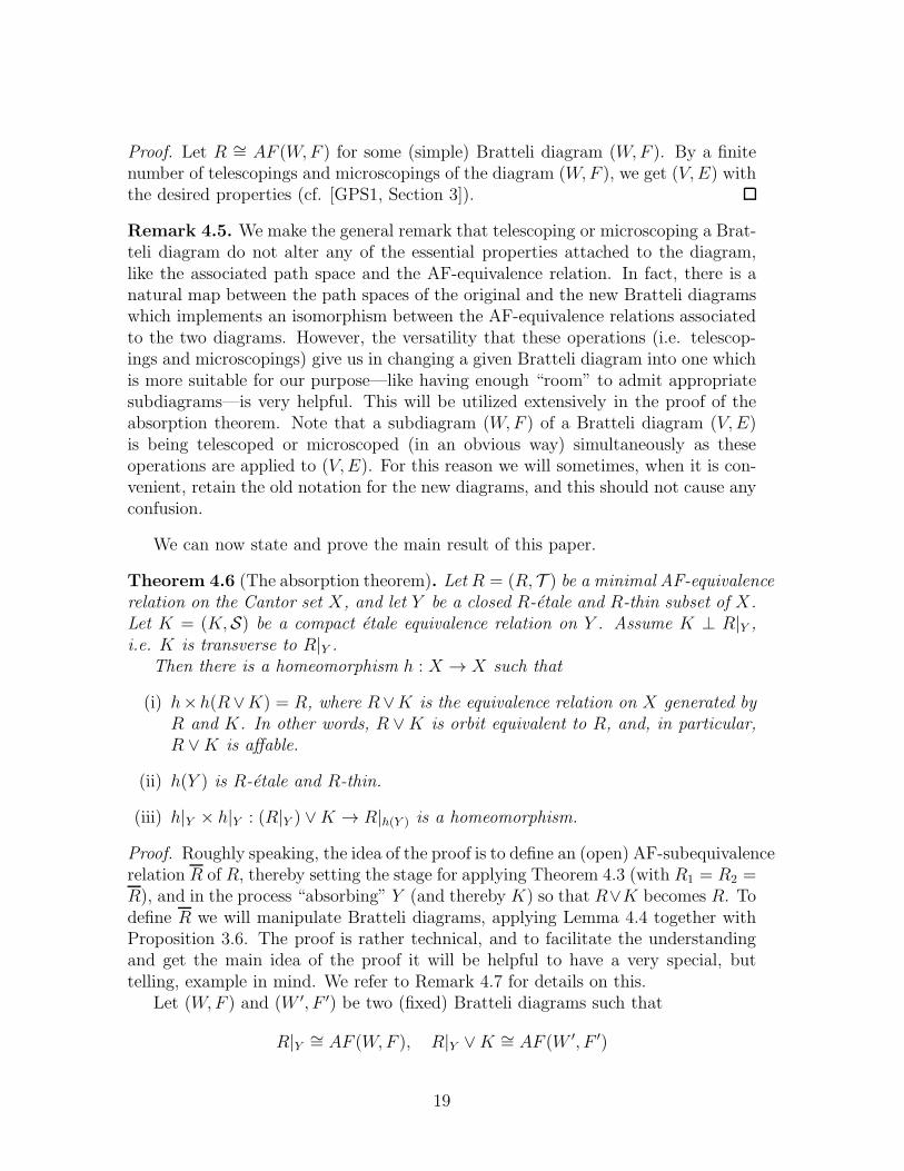
for Fk, cf. Proposition 3.6.) Using this we are going to construct a subdiagram of(V,E) which will consist of countable replicas of (W ′, F ′). This subdiagram will beinstrumental in defining the AF-subequivalence relation R of R that we alluded toabove. We first choose x∞ = (e1, e2, . . . ) ∈ X(V,E) such that t(en) /∈ Wn for all n.At level n we choose a replica of (W ′, F ′) “emanating” from the vertex t(en). Moreprecisely, we let (W ′, F ′)n denote the subdiagram of (V,E) consisting of the edgese1, e2, . . . , en and then (a replica of) (W ′, F ′) starting at the vertex t(en). This canbe done by (1) and (2). Also, by (1) we have enough “room” so that we may choosethe various (W ′, F ′)n’s such that at each level n ≥ 1, the vertex sets belonging

to (W , F ), (W ′, F ′)1, (W′, F ′)2, . . . , (W

′, F ′)n are pairwise disjoint. In Figure 5, wehave illustrated this.

By (2) it is easily seen that the subdiagram (L,G) of (V,E) whose edge set

consists of the edge set F and the union of the edge sets belonging to (W ′, F ′)n, n ≥1, is a thin subdiagram of (V,E), i.e. µ(X(L,G)) = 0 for all R-invariant probabilitymeasures µ (cf. Remark 4.5). Likewise, the subdiagram (L′, G′) whose edge setconsists of the union of the edge sets belonging to (W ′, F ′)n, n ≥ 1, is a thinsubdiagram.

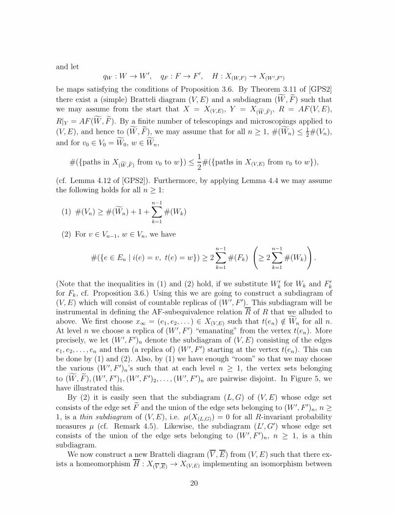
We now construct a new Bratteli diagram (V ,E) from (V,E) such that there ex-ists a homeomorphism H : X(V ,E) → X(V,E) implementing an isomorphism between

20

t

(V,E)

s

s

s

s

e1

e2

e3

e4

︸︷︷︸(W , F )

︸︷︷︸(W ′, F ′)1

︸︷︷︸(W ′, F ′)2

︸︷︷︸(W ′, F ′)3

Figure 5: Constructing subdiagrams of (V,E)

AF (V ,E) and the AF-subequivalence relation R of R that we want. The Bratteli di-agram (V ,E) will lend itself to apply Theorem 4.3 by, loosely speaking, transformingthe subdiagrams (W ′, F ′)n in (V,E) to replicas of (W,F ), thus making it possible to“absorb” the compact etale equivalence relation K. To construct (V ,E) from (V,E)we first replace each vertex v in Vn (for n ≥ 2) which belong to the union of thevertex sets of (W ′, F ′)1, (W

′, F ′)2, . . . , (W′, F ′)n−1, by the vertices in q−1

W ({v}). Weretain the other vertices in Vn, and thus we get V n. We set V 0 = V0 and V 1 = V1.There is an obvious map qV : V → V , respecting gradings, which is surjective, andwhich can be considered to be an extension of the map qW : W → W ′. Now wetransfer in an obvious sense the subdiagram (W , F ) of (V,E), again denoting it by

(W , F ), and so E will contain the edge set F . Similarly, in an obvious sense, wereplace (W ′, F ′)n by (W,F )n, n ≥ 1, where (W,F )n is defined in a similar way as wedefined (W ′, F ′)n. The new edge set E contains the collection of edges in (W,F )n,n ≥ 1, and so, in particular, the edges e1, e2, . . . lie in E. (We will denote the path(e1, e2, . . . ) again by x∞.) Furthermore, if e ∈ E is such that the vertices i(e) andt(e) do not lie in L′, then we retain e, and so e ∈ E. Let e ∈ E \G′, and let v = i(e)and w = t(e). If v ∈ L′, we replace e by #(q−1

V({v})) edges sourcing at each of the

vertices q−1V({v}) and ranging at the same vertex, where this vertex can be chosen

to be any vertex in q−1

V({w}). If v /∈ L′ and w ∈ L′, then we replace e by an edge

sourcing at v and ranging at an arbitrary vertex in q−1V({w}). However, we require

that the collection of these new edges will range at every vertex in q−1V({w}), as

we consider all edges e ∈ E \ G′ such that i(e) = v and t(e) = w, v ∈ Vn−1 and

21

t

(V,E)

s

s

s

s

e1

e2

e3

e4

︸︷︷︸(W , F )

s s

s s

s s

s s

︸︷︷︸(W ′, F ′)1

s

s

s

︸︷︷︸(W ′, F ′)2

s

s

︸︷︷︸(W ′, F ′)3

s

t

(V ,E)

s

s

s

s

e1

e2

e3

e4

︸︷︷︸(W , F )

s s

s s

s s

s s

︸︷︷︸(W,F )1

s s

s s

s s

︸︷︷︸(W,F )2

s s

s s

︸︷︷︸(W,F )3

s s❝

e

❝

×♣♣♣♣♣♣

f

×♣♣♣♣♣♣

Figure 6: Construction of the AF-subequivalence relation R ∼= AF (V ,E) of R =AF (V,E), cf. Remark 4.7

w ∈ Vn being fixed (n ≥ 1). By (2) there are sufficiently many edges e so that thiscan be achieved. So we have defined the edge set E, and we have done this in sucha way that (V ,E) is a simple Bratteli diagram by ensuring that for all v ∈ V n−1,w ∈ V n, there exists e ∈ E such that i(e) = v, t(e) = w. There is an obvious mapqE : E → E, respecting gradings, which is surjective, and which can be consideredto be an extension of the map qF : F → F ′. By the definition of qE and qV wehave that i(qE(e)) = qV (i(e)), t(qE(e)) = qV (t(e)) for e ∈ E. Also, using Proposi-tion 3.6 (ii), it is easy to show that qE : i−1({v}) → i−1({qV (v)}) is a bijection foreach v ∈ V . We deduce that the map (f1, f2, . . . , fn) 7→ (qE(f1), qE(f2), . . . , qE(fn))establishes a bijection between the finite paths of length n from the top vertices of(V ,E) and (V,E), respectively. We define the map H : X(V ,E) → X(V,E) by

x = (f1, f2, f3, . . . ) 7→ H(x) = (qE(f1), qE(f2), qE(f3), . . . ).

It is now routinely checked that H is a homeomorphism, and that H × H mapsAF (V ,E) isomorphically onto an AF-subequivalence relation R on X(V,E). ObservethatH mapsX(W,F )n ontoX(W ′,F ′)n for all n ≥ 1. (In fact, by obvious identifications,this map is the same as H : X(W,F ) → X(W ′,F ′) introduced earlier.) Also, H mapsX(fW, eF )(⊂ X(V ,E)) onto X(fW, eF )(⊂ X(V,E)), and H(x∞) = x∞.

We claim thatR = R ∨K1 ∨K2 ∨ . . . , (∗)

where Kn, n ≥ 1, is the CEER on X(W ′,F ′)n that corresponds to K via the ob-

22

vious map between X(W ′,F ′) and X(W ′,F ′)n . (We note for later use that, similarly,we have an obvious map between X(W,F ) and X(W,F )n.) Clearly the right handside of (∗) is contained in the left hand side. Now H|(W,F )n implements an embed-ding of AF ((W,F )n)(∼= AF (W,F ) ∼= R|Y ) into AF ((W ′, F ′)n)(∼= AF (W ′, F ′) ∼=(R|Y ) ∨K) which is transverse to Kn, and such that AF ((W ′, F ′)n) ∼= Kn ∨ (H ×H)(AF ((W,F )n)) (cf. Proposition 3.6). To prove that (∗) holds, let (x, y) ∈ R, andlet x, y ∈ X(V ,E) such that H(x) = x, H(y) = y. If the paths x and y agree from

level n on in X(V,E), then by the definition of H we must have that qE(fm) = qE(f′m)

and qV (i(fm)) = qV (i(f′m)) for all m > n, where x = (f1, f2, . . . ), y = (f ′

1, f′2, . . . ).

We first observe that x and y are cofinal paths in X(V ,E), that is, (x, y) ∈ AF (V ,E),if and only if i(fm) = i(f ′

m) for some m > n. Now it follows directly from the way weconstructed the Bratteli diagram (V ,E) from (V,E) that if qE(fm)(= qE(f

′m)) does

not belong to the edge set of a fixed (W ′, F ′)N for all m > n, then this situation willoccur, and so (H(x), H(y)) = (x, y) ∈ R. If on the other hand qE(fm) belongs to theedge set of a fixed (W ′, F ′)N for all m > n, then both fm and f ′

m belong to the edgeset of a fixed (W,F )N for all m > n. We can then find paths x and y in X(W,F )N (⊂X(V ,E)) which are cofinal with x and y, respectively, from level n on. Hence we will

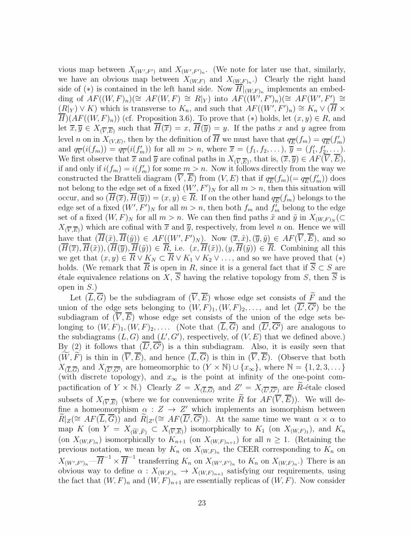
have that (H(x), H(y)) ∈ AF ((W ′, F ′)N). Now (x, x), (y, y) ∈ AF (V ,E), and so(H(x), H(x)), (H(y), H(y)) ∈ R, i.e. (x,H(x)), (y,H(y)) ∈ R. Combining all thiswe get that (x, y) ∈ R ∨KN ⊂ R ∨K1 ∨K2 ∨ . . . , and so we have proved that (∗)holds. (We remark that R is open in R, since it is a general fact that if S ⊂ S areetale equivalence relations on X , S having the relative topology from S, then S isopen in S.)

Let (L,G) be the subdiagram of (V ,E) whose edge set consists of F and theunion of the edge sets belonging to (W,F )1, (W,F )2, . . . , and let (L′, G′) be thesubdiagram of (V ,E) whose edge set consists of the union of the edge sets be-longing to (W,F )1, (W,F )2, . . . . (Note that (L,G) and (L′, G′) are analogous tothe subdiagrams (L,G) and (L′, G′), respectively, of (V,E) that we defined above.)By (2) it follows that (L′, G′) is a thin subdiagram. Also, it is easily seen that

(W , F ) is thin in (V ,E), and hence (L,G) is thin in (V ,E). (Observe that bothX(L,G) and X(L′,G′) are homeomorphic to (Y × N) ∪ {x∞}, where N = {1, 2, 3, . . . }(with discrete topology), and x∞ is the point at infinity of the one-point com-

pactification of Y × N.) Clearly Z = X(L,G) and Z ′ = X(L′,G′) are R-etale closed

subsets of X(V ,E) (where we for convenience write R for AF (V ,E)). We will de-fine a homeomorphism α : Z → Z ′ which implements an isomorphism betweenR|Z(∼= AF (L,G)) and R|Z′(∼= AF (L′, G′)). At the same time we want α × α tomap K (on Y = X(fW, eF ) ⊂ X(V ,E)) isomorphically to K1 (on X(W,F )1), and Kn

(on X(W,F )n) isomorphically to Kn+1 (on X(W,F )n+1) for all n ≥ 1. (Retaining theprevious notation, we mean by Kn on X(W,F )n the CEER corresponding to Kn on

X(W ′,F ′)n—H−1

×H−1

transferring Kn on X(W ′,F ′)n to Kn on X(W,F )n.) There is anobvious way to define α : X(W,F )n → X(W,F )n+1 satisfying our requirements, usingthe fact that (W,F )n and (W,F )n+1 are essentially replicas of (W,F ). Now consider

23

Y = X(fW, eF ), where X(fW, eF ) ⊂ X(V ,E). We have AF (W , F ) ∼= R|Y (which clearly

may be identified with R|Y ), and R|Y ∼= R|X(W,F )1(∼= AF (W,F )). Furthermore,

(R|Y )∨K ∼= (R|X(W,F )1)∨K1. The various isomorphism maps are naturally related,

and it follows that there exists α : X(fW, eF ) → X(W,F )1 satisfying our requirements.

(We omit the easily checked details.) Furthermore, note that α implements an iso-

morphism between (R|Y ) ∨ K and (R|X(W,F )1) ∨ K1. Also, H × H implements an

isomorphism between the latter and R|X(W ′,F ′)1. We define eventually α : Z → Z ′

by patching together the various α’s above, letting α(x∞) = x∞, and it is straight-forward to verify that this α satisfies all our requirements. By Theorem 4.3 thereexists an extension α : X(V ,E) → X(V ,E) of α which implements an automorphism of

R = AF (V ,E). Let h = H ◦ α ◦H−1. Then h is a homeomorphism on X = X(V,E).

Recall that H ×H(R) = R. By (∗) we have that

R ∨K = R ∨K ∨K1 ∨K2 ∨ . . . . (∗∗)

We note that

h× h(R) = (H ×H) ◦ (α× α) ◦ (H−1

×H−1)(R)

= (H ×H) ◦ (α× α)(R)

= (H ×H)(R)

= R.

Also,

h× h(K) = (H ×H) ◦ (α× α) ◦ (H−1

×H−1)(K)

= (H ×H) ◦ (α× α)(K)

= (H ×H)(K1)

= K1,

where we make the obvious identifications, referred to above, with K (respectivelyK1) as CEERs on X(fW, eF )(⊂ X(V,E)) and X(fW, eF )(⊂ X(V ,E)) (respectively, X(W ′,F ′)1(⊂

X(V,E)) and X(W,F )1(⊂ X(V ,E))). Similarly we show that h×h(Kn) = Kn+1 for n ≥ 1.By (∗∗) we get

h× h(R ∨K) = (h× h)(R) ∨ (h× h)(K) ∨ (h× h)(K1) ∨ . . .

= R ∨K1 ∨K2 ∨ . . .

= R.

This completes the proof of the main assertion, (i), of the theorem.Assertions (ii) and (iii) are now immediately clear since h(Y ) = X(W ′,F ′)1 and h|Y

(by definition of α|Y ) implements an isomorphism between (R|Y )∨K and R|h(Y )(∼=AF ((W ′, F ′)1)). This finishes the proof of the theorem.

24

Remark 4.7. In order to understand the idea behind the proof of the absorptiontheorem better, it is instructive to look at the simplest (non-trivial) case, namelywhen Y = {y1, y2} consists of two points y1 and y2, such that (y1, y2) /∈ R. (Even inthis simple case, the conclusion one can draw from the absorption theorem is highlynon-trivial.) The compact etale equivalence relation K on Y that is transverse toR|Y (= ∆Y ) is the following: K = ∆Y ∪ {(y1, y2), (y2, y1)}. The Bratteli diagrams

(W , F ) and (W,F ) for R|Y are trees consisting of two paths with no vertices incommon, except the top one. The Bratteli diagram (W ′, F ′) for (R|Y ) ∨ K startswith two edges forming a loop, and then a single path. In Figure 6 the scenario in thiscase is illustrated. (We have indicated how one constructs the new Bratteli diagram(V ,E) from (V,E) (where R = AF (V,E)) by exhibiting two specific edges e andf in E and how they give rise to new edges q−1

E({e}) and q−1

E({f}), respectively, in

E.) The example considered here corresponds to a very special case of transversalityarising from an action of the (finite) group G = Z/2Z = {0, 1}, where α1 : Y → Ysends y1 to y2 and y2 to y1 (cf. the comments after Definition 3.1). In the paper[GPS2] the general Z/2Z-action case is considered (even though it is formulatedslightly different there).

Remark 4.8. Theorem 4.6 is the key technical ingredient in the proof of the fol-lowing result:

Theorem ([GMPS]). Every minimal action of Z2 on a Cantor set is orbit equivalentto an AF-equivalence relation, and consequently also orbit equivalent to a minimalZ-action.

References

[GMPS] T. Giordano, H, Matui, I. F. Putnam and C. F. Skau, Orbit equivalencefor Cantor minimal Z2-systems, preprint. math.DS/0609668.

[GPS1] T. Giordano, I. F. Putnam and C. F. Skau, Topological orbit equivalenceand C∗-crossed products, J. Reine Angew. Math. 469 (1995), 51–111.

[GPS2] T. Giordano, I. F. Putnam and C. F. Skau, Affable equivalence relationsand orbit structure of Cantor dynamical systems, Ergodic Theory Dynam.Systems 24 (2004), 441–475.

[M] M. Molberg, AF-equivalence relations, Math. Scand. 99 (2006), 247–256.

[P] A. L. T. Paterson, Groupoids, inverse semigroups, and their operator alge-bras, Progress in Mathematics, 170. Birkhauser Boston, Inc., Boston, MA,1999.

25