3D Res. 02, 02003 (2011) 10.1007/3DRes.02(2011)3

3DR EXPRESS w

The 3D Hough Transform for Plane Detection in Point Clouds: A Review and a new Accumulator Design Dorit Borrmann • Jan Elseberg • Kai Lingemann • Andreas Nüchter

Received: 13 January 2011 / Revised: 13 February 2011 / Accepted: 10 March 2011 © 3D Research Center and Springer 2011

Abstract*The Hough Transform is a well-known method for detecting parameterized objects. It is the de facto standard for detecting lines and circles in 2-dimensional data sets. For 3D it has attained little attention so far. Even for the 2D case high computational costs have lead to the development of numerous variations for the Hough Transform. In this article we evaluate different variants of the Hough Transform with respect to their applicability to detect planes in 3D point clouds reliably. Apart from computational costs, the main problem is the representation of the accumulator. Usual implementations favor geometrical objects with certain parameters due to uneven sampling of the parameter space. We present a novel approach to design the accumulator focusing on achieving the same size for each cell and compare it to existing designs. Keywords Hough Transform, 3D laser scans, plane detection, indoor mapping 1. Introduction One of the main research topics in mobile robotics attends to create maps of the robot’s surroundings. Mapping is often achieved by matching separately collected partial views, e.g., laser scans. A laser scan is a set of distance values and taken by a robot at different positions, it represents the part of the environment that is observable from the current pose. The process of joining these partial

Dorit Borrmann1 ( ) • Jan Elseberg1 ( ) • Andreas Nüchter1 ( ) • Kai Lingemann2 ( ) 1Jacobs University Bremen gGmbH, 29759 Bremen, Germany Tel.: +49-421-200-3110; Fax.: +49-421-200-3103 2University of Osnabrück, 49069 Osnabrück, Germany e-mail: d.borrmann@jacobs-university.de, j.elseberg@jacobs-university.de, a.nuechter@jacobs-university.de, lingemann@informatik.uni-osnabrueck.de

views into a map is referred to as scan registration. Scan registration is subject to matching errors, sensor noise and systematic errors in the scans. The structure of indoor environments, however, usually comprises a large amount of planar surfaces. This can be exploited to reconstruct the real structure of the environment. Plane extraction, or plane fitting, is the problem of

modeling a given 3D point cloud as a set of planes that ideally explain every data point. The RANSAC algorithm is a general, randomized procedure that iteratively finds an accurate model for observed data that may contain a large number of outliers, (cf. Fischler and Bolles, 1981)1. Schnabel et al. (2007)2 have adapted RANSAC for plane extraction and found that the algorithm performs precise and fast plane extraction, but only if the parameters have been fine-tuned properly. For their optimization they use knowledge, that is not readily available in point cloud data, such as normals, neighboring relations and outlier ratios. Bauer and Polthier (2008)3 use the radon transform to detect planes in volume data. The idea and the speed of the algorithm are similar to that of the Standard Hough Transform. Poppinga et al. (2008)4 propose an approach to find planes with a combination of region growing and plane fitting. Other plane extraction algorithms are highly specialized for a specific application and are not in widespread use. Lakaemper and Latecki (2006)5 use an Expectation Maximization (EM) algorithm to fit planes that are initially randomly generated, Wulf et al.6 detect planes relying on the specific properties of a sweeping laser scanner and Yu et al.(2008)7 developed a clustering approach to solve the problem. Approaches that work on triangle meshes ask for

preprocessing of the original point data. Attene et al.(2006)8 fit geometric primitives into triangle meshes. The proposed prototype works for planes, cylinders and spheres but is easily extendible to other primitives. Starting from single triangles they extend the cluster into the direction that is best represented by one of the primitives.

2 3D Res. 02, 02003 (2011)

2. The 3D Hough Transform The Hough Transform (Hough, 1962)9 is a method for detecting parameterized objects, typically used for lines and circles. However, we focus on the detection of planes in 3D point clouds. Even though many Hough Transform approaches work with pixel images as input this is not a necessity. In our scenario a set of unorganized points in □³ are used as input and the output consists of parameterized planes. Planes are commonly represented by the signed distance ρ to the origin of the coordinate system and the slopes mx and my in direction of the x- and y-axis, respectively:

ρ++= ymxmz yx To avoid problems due to infinite slopes when trying to represent vertical planes, another usual definition, the Hesse normal form, uses normal vectors. A plane is thereby given by a point p on the plane, the normal vector n that is perpendicular to the plane and the distance ρ to the origin

ρρ =++=⋅= zzyyxx npnpnpnp Considering the angles between the normal vector and the coordinate system, the coordinates of n are factorized to

ρϕθϕϕθ =⋅+⋅⋅+⋅⋅ cossinsin sincos zyx ppp (1) with θ the angle of the normal vector on the xy-plane and φ the angle between the xy-plane and the normal vector in z direction as depicted in Fig. 1. φ, θ and ρ define the 3-dimensional Hough Space (θ, φ, ρ) such that each point in the Hough Space corresponds to one plane in ³. To find planes in a point set, one calculates the Hough

Transform for each point. Given a point p in Cartesian coordinates, we have to find all planes the point lies on, i.e., find all the θ, φ and ρ that satisfy Eq. (1). Marking these points in the Hough Space leads to a 3D sinusoid curve as shown in Fig. 2. The intersections of two curves in Hough Space denote the planes that are rotated around the line built by the two points. Consequently, the intersection of three curves in Hough Space corresponds to the polar coordinates defining the plane spanned by the three points. In Fig. 2 the intersection is marked in black. Given a set P of points in Cartesian coordinates, one transforms all points pi ∈ P into Hough Space. The more curves intersect in hj

(∈ θ, φ, ρ), the more points lie on the plane represented by hj and the higher is the probability that hj is actually extracted from P. 3. Hough methods 3.1 Standard Hough Transform For practical applications Duda and Hart (1971)10 propose discretizing the Hough Space with ρ′, φ′ and θ′ denoting the extent of each cell in the according direction in Hough Space. A data structure is needed to store all these cells with a score parameter for every cell. In the following, incrementing a cell refers to the increasing the score by +1. This data structure, called the accumulator, is described in more detail in Sec. 4. For each point pi we increment all the cells that are touched by its Hough Transform. The incrementation process is often referred to as voting, i.e., each point votes for all sets of parameters (θ, φ, ρ) that define a plane on which it may lie, i.e., if the euclidian

Fig. 1 Normal vector described by polar coordinates

Fig. 2 Transformation of three points from ³ into Hough Space (θ, φ, ρ). The intersection of the curve (marked in black) depicts the plane spanned by the three points. distance to the plane represented by the center of the cell is less than a threshold. The cells with the highest values represent the most prominent planes, the plane that covers the most points of the point cloud. Once all points have voted, the winning planes are

selected. Due to the discretization of the Hough Space and the noise in the input data it is advisable to search not only for one cell with a maximal score but for the maximum sum in a small region of the accumulator. Kiryati et al. (1991)11 use the standard practice for peak detection. In the sliding window procedure a small 3-dimensional window is defined that is designed to cover the full peak spread. The most prominent plane corresponds to the center point of a cube in Hough Space with a maximum sum of accumulation values. The steps of the procedure are outlined in Algorithm 1. Due to its high computation time (cf. Sec. 5.3) the

Standard Hough Transform is rather impractical, especially for real-time applications. Therefore numerous variants have been devised. Illingworth and Kittler (1988)12 give a survey on the early development and applications. Kälviäinen et al. (1995)13 compare modified versions of the Hough Transform aiming to make the algorithm more practical. Some of those procedures are described in the following subsections. Sec. 5.3 provides an evaluation of these methods with the goal to find the optimal variation

3D Res. 02, 02003 (2011) 3

for the task of detecting a previously unknown number of planes in a 3D point cloud.

Algorithm 1 Standard Hough Transform (SHT) 1: for all points in pi in point set P do 2: for all cells (θ, φ, ρ) in accumulator A do 3: if point pi lies on the plane defined by (θ, φ, ρ)

then 4: increment cell A(θ, φ, ρ) 5 : end if 6 : end for 7 : end for 8 : search for the most prominent cells in the

accumulator, that define the detected planes in P 3.2 Probabilistic Hough Transform The Standard Hough Transform is performed in two stages. First, all points pi from the point set P are transformed to Hough Space, i.e., the cells in the accumulator are incremented. This needs O(|P| · Nφ · Nθ) operations, where Nφ is the number of cells in direction of φ, Nθ in direction of θ and Nρ in direction of ρ, respectively, when calculation a single ρ corresponding to the plane on which a point pi is given φ and θ. Second, in a search phase the highest peaks in the accumulator are detected in O(Nρ · Nφ · Nθ). Since the size of the point cloud |P| is usually much larger than the number Nρ · Nφ · Nθ of cells in the accumulator array, major improvements concerning computational expenses are made by reducing the number of points rather than by adjusting the discretization of the Hough Space. To this end Kiryati et al. (1991)11 propose a probabilistic method for selecting a subset from the original point set. The adaptation of the SHT to the Probabilistic Hough Transform (PHT) is outlined in Algorithm 2.

Algorithm 2 Probabilistic Hough Transform (PHT) 1: determine m and T 2: randomly select m points to create Pm ⊂ P 3: for all points in m

ip in point set Pm do 4: for all cells (θ, φ, ρ) in accumulator A do 5: if point pi lies on the plane defined by (θ, φ, ρ) then 6: increment cell A(θ, φ, ρ) 7: end if 8: end for 9: end for 10: Search for the most prominent cells in the

accumulator, that define the detected planes in P m points (m < |P|) are randomly selected from the point

cloud P . These points are transformed into Hough Space and vote for the plane the points may lie on. The dominant part of the runtime is proportional to m · Nφ · Nθ. By reducing m, the runtime is reduced drastically. To obtain similar good results as with the Standard Hough

Transform it is important that a feature is still detected with high probability even when only a subset of m points is used. The optimal choice of m and the threshold T depend on the actual problem. Sensor noise leads to planes that appear thicker than they are in reality. Discretization of the Hough Space in combination with the sliding-window

approach helps to take care of this problem. The more planes are present in the point cloud the less prominent are peaks in the accumulator. The same effect appears, when objects are in the point cloud that do not consist of planes. Depending on these factors the optimal number m varies between data sets with different characteristics. 3.2.1 Adaptive Probabilistic Hough Transform The size for the optimal subset of points to achieve good results with the PHT is highly problem dependent. This subset is usually chosen much larger than needed to minimize the risk of errors. Some methods have been developed to determine a reasonable number of selected points. The Adaptive Probabilistic Hough Transform (APHT) (Ylä-Jääski and Kiryati, 1994)14 monitors the accumulator. The structure of the accumulator changes dynamically during the voting phase. As soon as stable structures emerge and turn into significant peaks voting is terminated. Only those cells need to be monitored after each voting

process that have been touched. The maximal cell of those is identified and considered for plane extraction. If several cells have the same high score, one of them is chosen. A list of potential maximum cells is updated. A comparison of consecutive peak lists allows for checking the consistency of the peak rankings in the lists. Algorithm 3 outlines this procedure.

Algorithm 3 Adaptive Probabilistic Hough Transform (APHT) 1: while stability order of Sk is smaller than threshold tk

and maximum stability order is smaller than threshold tmax do

2: randomly select a small subset Pm ⊂ P of size n 3: for all points m

ip in Pm do 4: vote for the cells in the accumulator

5 : choose maximum cell from the incremented cells and add it to active list of maxima

6 : end for 7: merge active list of peaks with previous list of

peaks 8: determine stability order 9: end while

To speed up the process the list update is only performed

after a small batch of points has voted. The list of peaks is limited in size and incrementally ordered by the value of the cells. When updating the list with a peak the coordinates of the peak are taken into account. If two peaks lie in the spatial neighborhood of each other, the lower one is disregarded or removed from the list. In the early stages of the algorithm changes in the order of peaks are frequent. As updating proceeds, the structure of the accumulator becomes clearer. The stopping rule for the algorithm is determined by the stability of the most dominant peaks. A set Sk of k peaks in the list is called stable, if the set contains all largest peaks before and after one update phase. The order within the set is insignificant for the stability. The number mk of consecutive lists in which Sk is stable is called the stability order of Sk. The maximum stability count is the

4 3D Res. 02, 02003 (2011)

cardinality k of the set Sk with the highest stability order. In case there are two sets with the same stability order the one with the higher cardinality is preferred. The stability order of the set Sk that has the maximum stability count is referred to as maximum stability order. The stopping rule for detecting exactly one plane is if the

stability order of S1 exceeds a predetermined threshold. For detecting k objects the stability order of Sk has to exceed a predetermined number. Detecting an arbitrary number of planes using several iterations with a fixed k may lead to long runtimes. Thus one recommends letting the program run until the maximum stability order reaches a threshold. The maximum stability count is then the number of found objects. 3.2.2 Progressive Probabilistic Hough Transform The Progressive Probabilistic Hough Transform (PPHT) (Matas et al., 1998) 15 calculates stopping times for random selection of points dependent on the number of votes in one accumulator cell and the total number of votes. The background of this approach is filtering those accumulation results that are due to random noise. The algorithm stops whenever a cell count exceeds a threshold of s points that could be caused by noise in the input. The threshold is calculated each time a point has voted. It is predicated on the percentage of votes for one cell from all points that have voted. Once a geometrical object is detected, the votes from all points supporting it are retracted. The stopping rule is exile as stopping at any time leads to

useful results. Features are detected as soon as the contents of the accumulator allow a decision. If the algorithm is not stopped it runs until no points are left in the input set. This happens when all points have either voted or have been found to lie on an already detected plane. Even if the algorithm is allowed to knish early it does not mean that all points must have voted. Depending on the structure of the input many points may have been deleted before voting because they belong to a plane that was detected. The PPHT is outlined in Algorithm 4. 3.3 Randomized Hough Transform Up et al. (1990)16 describe the Randomized Hough Transform (RHT) that decreases the number of cells touched by exploiting the fact that a curve with n parameters is defined by n points. For detecting planes, three points from the input space are mapped onto one point in the Hough Space. This point is the one corresponding to the plane spanned by the three points. In each step the procedure randomly picks three points p1, p2 and p3 from the point cloud. The plane spanned by the three points is calculated as ρ = n · p1 = ((p3 − p2) × (p1 − p2)) · p1. φ and θ are calculated as explained in Section 2 and the corresponding cell A(θ, φ, ρ) is accumulated. If the point cloud consists of a plane with θ, φ, ρ, after a certain number of iterations there will be a high score at A(θ, φ, ρ). When a plane is represented by a large number of points, it

is more likely that three points from this plane are randomly selected. Eventually the cells corresponding to actual planes

receive more votes and are distinguishable from the other cells. If points are very far apart, they most likely do not belong to one plane. To take care of this and to diminish errors from sensor noise a distance criterion is introduced: distmax (p1, p2, p3) ≤ distmax, i.e., the maximum point-to-point distance between p1, p2 and p3 is below a fixed threshold; for minimum distance, analogous. The basic algorithm is structured as described in Algorithm 5.

Algorithm 4 Progressive Probabilistic Hough Transform (PPHT) 1: while still enough points in P do 2: randomly select a point pi from point set P 3: calculate threshold t 4: for all cells (θ, φ, ρ) in accumulator A do 5: if point pi lies on the plane defined by (θ, φ, ρ)

then6: increment cell A(θ, φ, ρ) 7: end if 8: end for 9: remove point pi from P and add it to Pvoted 10: if highest accumulated cell is higher than threshold

t then 11: select all points from P and Pvoted that are close to

the plane defined by the highest peak and add them to Pplane

12: search for the largest connected region Pregion in Pplane

13: remove from P all points that are in Pregion 14: for all point pj that are in Pvoted and Pregion do 15: unvote pj from the accumulator 16: remove pj from Pvoted 17: end for 18: if the area covered by Pregion is larger than a

threshold then 19: add Pregion to the output list 20: end if 21: end if 22: end while

Algorithm 5 Randomized Hough Transform (RHT)

1: while still enough points in point set P do 2: randomly pick three points p1, p2, p3 from the set of

points P 3: if p1, p2 and p3 fulfill the distance criterion then 4: calculate plane (θ, φ, ρ) spanned by p1, p2, p3 5: increment cell A(θ, φ, ρ) in the accumulator space 6: if the counter |A(θ, φ, ρ)| equals threshold t then 7: (θ, φ, ρ) parameterize the detected plane 8: delete all points close to (θ, φ, ρ) from P 9: reset the accumulator 10: end if 11: else 12: continue 13: end if 14: end while

The RHT has several main advantages. Not all points have

to be processed, and for those points considered no complete Hough Transform is necessary. Instead, the intersection of three Hough Transform curves is marked in the accumulator to detect the curves one by one. Once there

3D Res. 02, 02003 (2011) 5

are three points whose plane leads to an accumulation value above a certain threshold t, all points lying on that plane are removed from the input and hereby the detection efficiency be increased. Since the algorithm does not calculate the complete Hough Transform for all points, it is likely that not the entire Hough Space needs to be touched. There will be many planes on which no input point lies. This calls for space saving storage procedures that only store the cells actually touched by the Hough Transform. 3.4 Summary of Hough Methods All methods of the Hough Transform described in this section have in common that they transform a point cloud into the Hough Space and detect planes by counting the number of points that lie on one plane represented as one cell in an accumulator. Table 1 summarizes the features in which the methods differ.

Table 1 Distinctive characteristic of Hough Transform methods.

SHT PHT PPHT APHT RHT

complete/ deterministic

+ - - - -

stopping rule - - + + + adaptive stopping rule

- - + ++ -

delete detected planes from point set

- - + - +

touch only one cell per iteration

- - - - +

easy to implement + + + - + In the SHT the complete HT is performed for all points. This makes it the only deterministic Hough variant. The PPHT, APHT and RHT have a stopping rule. While for the RHT the stopping rule is a simple threshold, e.g., number of points left in the point cloud or number of planes detected, the PPHT has a stopping rule that is based on the number of points already processed. Thus the algorithm is less sensitive to noise in the data. The most sophisticated stopping rule is applied in the APHT. Here the stability of several maxima is monitored over time during the voting phase making the algorithm more robust towards the negative effects of randomized point selection. In the PPHT and the RHT points are removed from the point cloud once a plane they lie on is detected. This does not only speed up the algorithm due to the decreasing number of points but also lowers the risk of detecting a false plane that goes through these points, especially in noisy data. The main advantage of the RHT is that in each iteration only one cell is touched. By avoiding performing the complete Hough Transform the large amount of cells that correspond to planes only represented by very few points is most likely not to be touched by the RHT. The main disadvantage of the APHT is its implementation. While the other methods are straightforward to implement, the necessity to maintain a list of maxima that also takes into account neighborhood relations leads to a higher implementation complexity. A comparison of the performance of the Hough Transform methods follows in Sec. 5.3.

4. New accumulator design

(a) Array (b) Cube

(c) Octahedron (d) Ball

Fig. 3 (a) – (d): Mapping of the accumulator designs onto the unit sphere. (a) Accumulator array. Also illustrated is the calculation of the length of a longitude circle at φi that determines the discretization for the ball design. The segment in question is the darker colored one. (b) Accumulator cube (taken from Censi and Carpin (2009)17). (c) Accumulator octahedron. (d) Accumulator ball. Without prior knowledge of the point cloud it is almost impossible to define proper accumulator arrays. An inappropriate accumulator, however, leads to detection failures of some specific planes and difficulties in finding local maxima, displays low accuracy, large storage space, and low speed. A tradeoff has to be found between a coarse discretization that accurately detects planes and a small number of cells in the accumulator to decrease the time needed for the Hough Transform. Choosing a cell size that is too small might also lead to a harder detection of planes in noisy laser data. 4.1 Accumulator array For the standard implementation of the 2-dimensional Hough Transform (Duda and Hart, 1971)10 the Hough Space is divided into Nρ × Nφ rectangular cells. The size of the cells is variable and is chosen problem dependent. Using the same subdivision for the 3-dimensional Hough Space by dividing it into cuboid cells results in the patches seen in Fig. 3(a). The cells closer to the poles are smaller and comprise less normal vectors. This means voting favors the larger equatorial cells. 4.2 Accumulator cube

Censi and Carpin (2009)17 propose a design for an accumulator that is a tradeoff between efficiency and ease of implementation. Their intention is to define correspondences between cells in the accumulator and small patches on the unit sphere with the requirement that the difference of size between the patches on the unit sphere is negligible. Their solution is to project the unit sphere S²

6 3D Res. 02, 02003 (2011)

onto the smallest cube that contains the sphere using the diffeomorphism

∞→ sss / cube, S: a2ϕ

Each face of the cube is divided into a regular grid. Fig. 3(b) shows the resulting patches on the sphere. Zaharia and Preteux (2002)18 use a similar design that focuses on the same decomposition in the direction of all coordinate axes. This is achieved when partitioning the Hough Space by projecting the vertices of any regular polyhedron onto the unit space. The level of granularity can be varied by recursively subdividing each of the polyhedral faces. An example is given in Fig. 3(c). Each octrahedron has the same subdivision. While both of these designs are invariant against rotation of 90° around any of the coordinate axes, they have one major drawback in common: when mapping the partitions on the unit sphere the patches appear to be unequally sized, favoring those planes represented by the larger cells. 4.3 Accumulator ball The commonly used designs share one drawback, i.e., the irregularity between the patches on the unit sphere. Next, we present our novel design for the accumulator with the intention of having the same patch size for each cell. To this end, the resolution in terms of polar coordinates has to be varied dependent on the position on the sphere. Thus, the sphere is divided into slices (cf. Fig. 3(a)). The resolution of the longitude φ is kept as for the accumulator array. φ′ determines the distance between the latitude circles on the sphere, e.g., the thickness of the slices. Depending on the longitude of each of the latitude circles the discretization has to be adapted. One way of discretization is to calculate the step width θ′ based on the size of the latitude circle at φi. The largest possible circle is the equator located at φ = 0. For the unit sphere it has the length maxl = 2π. The length of the latitude circle in the middle of the segment located above φi is given by lengthi = 2π(φi + φ′). The step width in θ direction for each slice is now computed as

θϕθ Ni

li ⋅

⋅°=′

lengthmax360

The resulting design is illustrated in Fig. 3(d). The image shows clearly that all accumulator cells are of similar size. Compared to the previously explained accumulator designs, the accumulator cube and the polyhedral accumulator, a possible drawback becomes obvious when looking at the projections on the unit sphere. The proposed design lacks invariance against rotations of multiples of 90°. This leads to a distribution of the votes to several cells. In practice however this problem is negligible since in most cases the planes to be detected do not align perfectly with the coordinate system, as will be shown in the experimental evaluation. 5. Experimental evaluation In this section a comparison of the accumulator designs is followed by an evaluation of the different Hough methods against each other. The experiments are performed on an

Intel Q9450 2.66 GHz processor with 4 GB RAM using one thread. 5.1 Comparison of accumulator designs The different designs for storing the votes of the Hough Transform are compared in this section using simulated as well as real 3D laser scans. The simple array structure where φ and θ are discretized uniformly is the simplest way of discretizing the Hough Space. It is interesting to investigate whether the obvious flaws of this design come into effect in practical applications or if they are negligible. Second, out of the two designs that focus on symmetry with respect to the coordinate system we chose the cuboid design over the polyhedral design, since both designs seem to have similar characteristics and the cuboid design appears to be easier to manage. Third, the design of our accumulator ball with different discretization for each latitude slice of the unit sphere is evaluated against those other two designs. 5.1.1 Evaluation using simulated data

(a) (b) (c)

(d) (e) (f)

Fig. 4 Left to right: array, cube, ball design of the accumulator. The input data is the modeled cube rotated by (0, 0, 0) (left) and (45, 45, 45) (right). The darker the color, the higher is the count for that cell. For easier evaluation we reduce the experimental setup to a simple test case. A cube with a side length of 400 cm is placed around the origin. Each side consists of 10,000 points which are randomly distributed over the entire face of the cube with a maximal noise of 10 cm. Different rotations are applied to the cube to simulate different orientations of planes. The advantage of using this simple model is the existence of ground truth data for the actual

3D Res. 02, 02003 (2011) 7

planes. The cube possesses a perpendicular structure which is characteristic for most man-made indoor environments. As pointed out in Section 4 rotating the cube poses challenges to the accumulators as the sides are not symmetrically aligned with the coordinate axes anymore.

Quantitative evaluation: The first experiment presents a graphical investigation of the ability of the accumulator designs to correctly detect planes in the given point cloud. For this purpose we apply the SHT to the cube. To achieve comparable results the number of cells for each accumulator needs to be approximately the same. Nρ = 100 with a maximal distance of 600. For the accumulator ball we use Nφ = 45 and Nθ = 90. This means that the slice around the equator consists of 90 patches. The total number of cells is 257,100. The accumulator cube has a total number of 264,600 cells when using 21 × 21 cells on each face. The simple accumulator is discretized with Nφ = 38 and Nθ = 76 leading to 288,800 cells.

In Fig. 4 the accumulators are plotted after applying 100,000 iterations of the RHT. For better visibility only the slice with 198 < ρ < 204 is shown, i.e., the distance that the planes have. The votes are drawn in blue, the darker a cell, the more votes it has received. The first three images show the results for the perfectly aligned cube and the cube rotated by 45° around each axis. The images show that for the accumulator array the two planes corresponding to the highest and lowest φ values do not show up. For the ball design the peaks show up, but are not as high as the peaks around the equator. In practice this means that the several cells along the equator have higher votes as the cells around the poles and are therefore earlier detected as planes. The images (d)–(f) show the same experiments with the rotated cube. The six peaks that show up in the accumulator array vary in color. The same holds true for the cube. The peaks close to the corners of the cube (the faces of the accumulator are marked in different colors) show a lighter blue. These are the regions where the patches have the smallest size. The result is that planes corresponding to those cells are less likely to be detected. For the ball design the peaks are most evenly colored in this scenario. This supports the previously mentioned assumption that the ball design is the best for detecting arbitrary planes due to its characteristic of having evenly sized patches in the Hough space.

For the next test case we use the laser scan model of the cube rotated by (10, 10, 10) and apply the SHT to it using all three different accumulators. After the voting phase in the SHT, the peaks in the accumulator have to be found and a decision has to be made which of those peaks correspond to actual planes in the input data. As seen in Fig. 4 the votes for one plane spread over a small region in the Hough Space. To pick the best representation out of one of these regions we implemented a simple peak search strategy that is applied after voting. Starting in one corner of the accumulator, we run over the complete space with a small window, in this experiment 8 × 8 × 8 cells. Within this window all values but the highest one are set to zero. This simple strategy might favor certain maxima but in our experiments this fact showed little influence on the results. For the accumulator cube we ran over each face separately. In the accumulator ball each slice consists of a different number of cells. This might cause problems when applying this windowed peak search. However, due to the small

difference in size of two neighboring slices the covered region is not regularly shaped but still connected.

(a) (b) (c)

(d) (e) (f)

(g) (h) (i)

Fig. 5 Planes detected by the SHT using different accumulators. Accumulator array (a) - (c): (a) 20 planes with the highest score. (b) After peak search procedure, all planes with more than 90% of the maximal score. (c) The six planes with the highest score (more than 80% of the maximal score). Accumulator cube (d) - (f): (d) 20 planes with the highest score (e) After peak search procedure, all planes with more than 90% of the maximal score. (f) The six planes with the highest score ( > 88%). Accumulator ball (g) - (h): (g) 20 planes with the highest score. Note that the first six represent already all different faces of the cube. (h) After peak search procedure, all planes with more than 90% of the maximal score. The resulting planes correspond to the six faces of the cube. (i): The data set used for the experiment, a cube with side length 400, placed around the origin. Each side consists of 10000 points randomly distributed with a maximal noise of 10.

The resulting planes are shown in Fig. 5. The first image for each accumulator depicts the 20 planes with the highest score using no peak search strategy. Secondly, after applying the peak search strategy, for all accumulators all planes with a count up to 90 % of the highest score are considered to be actual planes. For the accumulator ball these planes are very close to the six faces of the cube model. For the accumulator cube only two planes are above the threshold. For the accumulator array the back and the bottom face are not among the top 90 % while the front appears three times. For the cube the threshold to correctly detect all six faces of the model is 88 %. For the array all six faces of cube have a score above 80 %.

Qualitative evaluation: The demands towards the HT are twofold. First, the planes need to be easily detected, i.e., each plane is represented by exactly one dominant maximum in the accumulator. In the example this means that each of the six highest peaks corresponds to one face of the cube. Second, the highest peak for each face is as close as possible to the ground truth of the plane. Fig. 6 shows an evaluation of the three different accumulator designs with respect to these aspects. On the left the ability to correctly detect all six planes is depicted. Nine different rotations are applied to the cube. The bars indicate the number of incorrectly detected planes, i.e., if the six highest peaks

8 3D Res. 02, 02003 (2011)

Fig. 6 Left: Number of incorrectly detected planes on a logarithmic scale. Right: Angle error of the detected planes. Each set of bars represents one orientation of the cuboid laser scan model rotated by (αx, αy, αz) as denoted underneath each set. αx is the rotation around the x-axis, αy around the y-axis and αz around the z-axis. correspond to the six different faces of the cube, the error is zero. Each time the next highest peak corresponds to an already detected plane before every single face of the cube is represented by one peak, the error is incremented by one. The results show clearly that the simple array structure has significant problems to correctly identify the six cube faces. It totally fails when the cube is aligned with the coordinate system, as motivated in Section 4. The uneven sizes of the patches lead to an uneven distribution of peaks against favor of the planes parallel to the xy-plane. This comes mostly in effect when the cube is aligned with the coordinate system, when rotated the effects diminish but do not disappear.

In Fig. 4 it became obvious that the accumulator ball has problems detecting planes that are parallel to the xy-plane. If the cap of the ball is divided into several patches, more cells intersect at the poles than at the other parts of the accumulator. This leads to distribution of the votes over all these patches, decreasing the count for each of these cells. This problem is solved by creating a circular cell around the pole that has the desired size of the patches and proceed with the rest of the sphere in the same manner as before. Using this design the ball and the cube show similar performance. The ball performs better in some test cases, the cube in others. On average the ball design slightly outperforms the cube.

The chart on the right of Fig. 6 shows the sum of the angle errors for the detected planes. For each side of the cube the cell with the highest vote is used and the angle between the normal vector and the ground truth normal vector of the plane is calculated as error. The results show only small, negligible differences between the different accumulator designs. This indicates that once a plane is detected correctly the parameters are calculated equally well with each accumulator design. 5.1.2 Evaluation using real laser data To show the applicability of the Hough Transform to real laser data, we apply the RHT to a laser scan of an empty office. The result is shown in Fig. 7. All planes were correctly detected within less than 600 ms on an Intel Core 2 Duo 2.0 GHz processor with 4 GB RAM. For further evaluation on the applicability of the Hough Transform see (Borrmann and Elseberg, 2009)19.

Fig. 7 Scan of an empty office with planes detected (RHT).

5.2 Standard Hough Transform For 2D data the Standard Hough Transform is one of the standard methods for detecting parameterized objects. But even there, enormous computational requirements have lead to the emerge of more and more methods to accelerate the Hough Transform without loss of precision. For 3D data the requirements increase drastically. Therefore, we are dealing with the question of applicability of the Standard Hough Transform in the 3D case.

For easier evaluation we use a simulated laser scan model. A cube with a side length of 400 cm is placed around the origin. Each side consists of 10,000 points which are randomly distributed over the entire face of the cube with a maximal noise of 10 cm. Different rotations are applied to the cube to simulate different orientations of planes. Fig. 5 shows the data set rotated by 10° around each axis as well as the results after applying the SHT to it. Shown are the planes with a count up to 90 % of the highest score. These planes are very close to the six faces of the cube model. 5.3 Evaluation of Hough Transform methods To evaluate the different Hough methods we use the same setup for each method. The first experiment investigates how well the Hough methods detect one plane. We express this in terms of mean and variance of the result. Using the cuboid accumulator design and only one face of the laser scan cube model we consider only one face of the accumulator. The accumulator face is divided into 22×22 faces. The slice considered is the one with 198 < ρ < 204. The mean is calculated as the sum of all accumulator cells weighed by the score of that cell and divided by the number of cells. The error plotted is the distance between the calculated mean and the supporting point of the optimal

3D Res. 02, 02003 (2011) 9

plane representation of the face. The variance illustrates the distribution of the values in the accumulator face in relation

to the calculated mean.

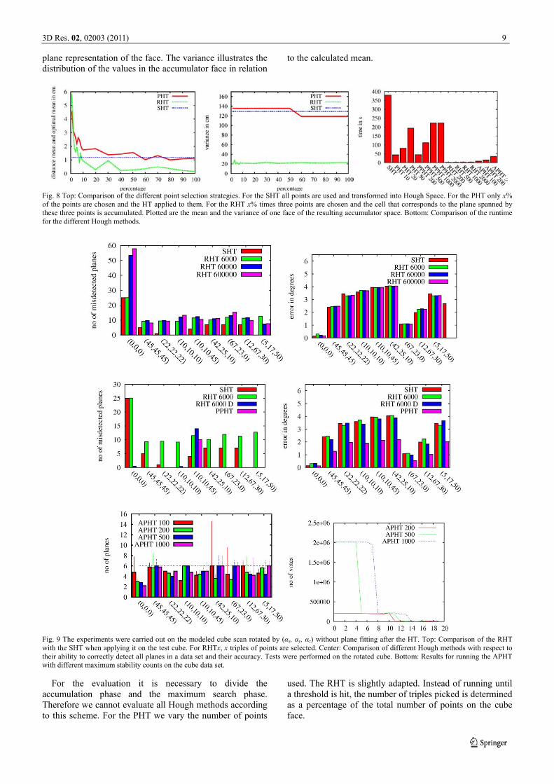
Fig. 8 Top: Comparison of the different point selection strategies. For the SHT all points are used and transformed into Hough Space. For the PHT only x% of the points are chosen and the HT applied to them. For the RHT x% times three points are chosen and the cell that corresponds to the plane spanned by these three points is accumulated. Plotted are the mean and the variance of one face of the resulting accumulator space. Bottom: Comparison of the runtime for the different Hough methods.

Fig. 9 The experiments were carried out on the modeled cube scan rotated by (αx, αy, αz) without plane fitting after the HT. Top: Comparison of the RHT with the SHT when applying it on the test cube. For RHTx, x triples of points are selected. Center: Comparison of different Hough methods with respect to their ability to correctly detect all planes in a data set and their accuracy. Tests were performed on the rotated cube. Bottom: Results for running the APHT with different maximum stability counts on the cube data set.

For the evaluation it is necessary to divide the accumulation phase and the maximum search phase. Therefore we cannot evaluate all Hough methods according to this scheme. For the PHT we vary the number of points

used. The RHT is slightly adapted. Instead of running until a threshold is hit, the number of triples picked is determined as a percentage of the total number of points on the cube face.

10 3D Res. 02, 02003 (2011)

The average of running 20 times with each setting is plotted in Fig. 8. With more than 10% the RHT outperforms the SHT. Starting from 30% the error of the PHT is close to that of the SHT. The variance of the SHT and the PHT are close together. The RHT has a significantly smaller variance. Interpreting the results suggests that applying the PHT with at least 30% of the points leads to results that sufficiently represent the input data. The results for the RHT have to be considered very carefully as the RHT benefits from the simplicity of the input data. If using only one plane as input the RHT has hardly any variance. Selecting three points from different planes leads to more erroneous results. Due to that a more differentiated test of the RHT is needed.

We use 9 different rotations of the modeled cube to compare the different Hough methods further. The accumulator used for this evaluation is the ball structure with Nφ = 45, Nθ = 90 and Nρ = 100. The average of 20 test runs for all Hough methods is plotted in Fig. 9. Shown is the number of misdetected planes until each face of the cube is found exactly once. The quality of the detected planes is calculated as the angle between the perfect normal vector and the first normal vector of each detected face. The differences of the angle error are within a negligible range. The number of incorrectly detected planes differs depending on the rotation of the point cloud. In all cases the SHT performs noticeably better than the adapted version of the RHT (top). However, in its original version the RHT (cf. Section 3.3) has a phase where the accumulator is reset and the points that belong to an already detected plane are deleted.

The results for the original RHT are shown in Fig. 9 (middle) along with results on the same experiment for the PPHT. The thresholds for the maximal accumulator counts for RHT and PPHT are set to 1,000. The results show that when deleting the detected planes in between the accuracy of the HT with respect to finding each plane exactly once is significantly improved. In most cases the first six detected planes correspond to six different faces of the cube. Noticeable is, that for the PPHT also the error in the orientation of the normal vector is significantly smaller. In practice the difference does not play an important role if plane fitting is used in order to diminish the negative effects of the discretization.

Like the RHT and PPHT the APHT includes a stopping rule for when to stop transforming points into Hough Space. Instead of detecting a single peak the stability of many peaks is analyzed. For detecting an unknown number of planes a maximum stability count at which the algorithm stops is set.

Fig. 9 (bottom) shows a brief analysis of the APHT. The graph on the right shows an exemplary distribution of accumulator counts when using a list of 20 maxima and different maximum stability counts as stopping rule. It becomes clear that the counts between the detected planes and the not detected planes become very distinctive. However, the algorithm detects 8 planes for the cube data set. The left image shows a more thorough evaluation. The lines indicate the number of planes detected by the algorithm averaged over 20 runs. The boxes show the number of planes of this list that are a best representation for a cube faces. It is clear that the algorithm gives a close

prediction of the actual planes but fails to correctly identify all planes in almost any case.

The remaining question is how far the different methods improve the runtime of the algorithm. For this we run each algorithm 20 times, measure the time needed and plot the average time. For the variations we use different settings. The PHT is run with 10, 20 and 50 percent of the points. For the RHT and the PPHT maximal counts of 200, 500, 1,000 and 2,000 are used. For the APHT we used a maximum stability count of 100, 200 and 500. Since the RHT and PPHT have intermediate phases for deleting the points for one detected plane we include this phase into the measurements for all algorithms. This means the runtime includes the voting phase in the accumulator, the maximum search, plane fitting and creation of the convex hull of the planes.

Fig. 8 shows the runtimes for the different Hough algorithms. All variations drastically improve the runtime of the HT compared to the SHT. As expected, the runtime for the PHT decreases proportional to the decrease of points. The PPHT yields the best quality results. The runtime is similar to the PHT. However, the experiments that lead to the results of the quality evaluation were done with a maximal accumulator count of 100 which leads to even shorter runtimes, as depicted in the graph. Considering that the PHT needs to be run with at least 30% of the points, the PPHT is considerably faster. The APHT needs astonishingly short runtimes. Nevertheless, in the configurations used in the experiments the APHT was not able to reliably detect all six planes. The RHT outperforms all the other HT methods by far concerning runtime. Considering that the quality of the detected planes was only slightly behind the PPHT the RHT seems to be the method of choice for detecting an unknown number of planes in a laser scan map in reasonable time. 5.4 Comparison with region growing We have analyzed the Hough Transform and other effective methods for plane detection. Since a detailed comparison with respect to RANSAC is given in (Tarsha-Kurdi et al., 2007)20 we focus here on region growing methods. First, we evaluate against the approach by Poppinga et al. (2008)4. Their approach works for point clouds in Cartesian coordinates, which are generated from range images. It combines region growing and incremental plane fitting followed by a polygonization step. The algorithm starts with a randomly selected point from the point cloud and its nearest neighbor. Iteratively this set is enlarged by adding points that have the smallest distance to the current region, are close to the optimal plane through the points of the region, and do not lift the mean square error of the optimal plane above a threshold. Regions with a too small number of points are discarded. To speed up the algorithm the 8 neighbors in the range image of each newly added point are inserted into a priority queue from which the next point is chosen. An update strategy for the plane fitting avoids expensive recalculations in each step. A second state-of-the-art method is the mesh segmentation

by fitting of primitives (HFP – hierarchical fitting primitives) by Attene et al. (2006)8. The algorithm works on

3D Res. 02, 02003 (2011) 11

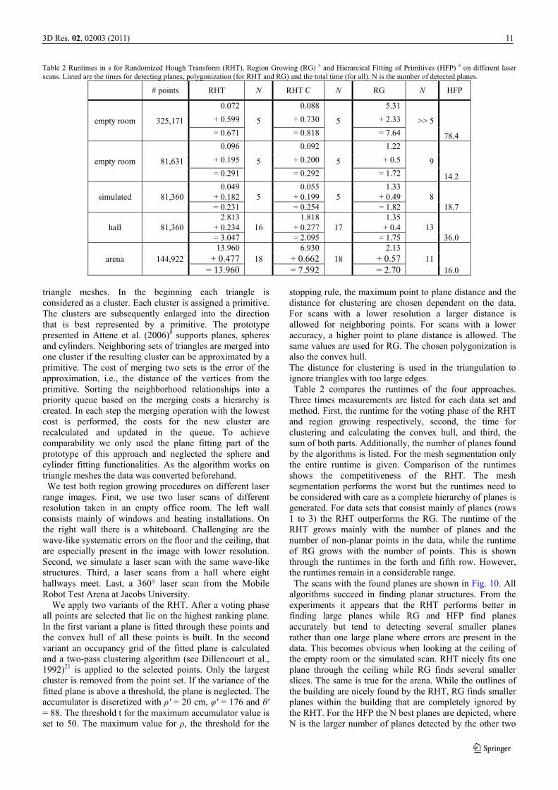
Table 2 Runtimes in s for Randomized Hough Transform (RHT), Region Growing (RG) 4 and Hierarcical Fitting of Primitives (HFP) 8 on different laser scans. Listed are the times for detecting planes, polygonization (for RHT and RG) and the total time (for all). N is the number of detected planes.

# points RHT N RHT C N RG N HFP

empty room 325,171

0.072

5

0.088

5

5.31

>> 5

78.4

+ 0.599 + 0.730 + 2.33 = 0.671 = 0.818 = 7.64

empty room 81,631

0.096

5

0.092

5

1.22

9

14.2

+ 0.195 + 0.200 + 0.5 = 0.291 = 0.292 = 1.72

simulated 81,360 0.049

5 0.055

5 1.33

8 18.7

+ 0.182 + 0.199 + 0.49 = 0.231 = 0.254 = 1.82

hall 81,360 2.813

16 1.818

17 1.35

13 36.0

+ 0.234 + 0.277 + 0.4 = 3.047 = 2.095 = 1.75

arena 144,922 13.960

18 6.930

18 2.13

11 16.0

+ 0.477 + 0.662 + 0.57 = 13.960 = 7.592 = 2.70

triangle meshes. In the beginning each triangle is considered as a cluster. Each cluster is assigned a primitive. The clusters are subsequently enlarged into the direction that is best represented by a primitive. The prototype presented in Attene et al. (2006)8 supports planes, spheres and cylinders. Neighboring sets of triangles are merged into one cluster if the resulting cluster can be approximated by a primitive. The cost of merging two sets is the error of the approximation, i.e., the distance of the vertices from the primitive. Sorting the neighborhood relationships into a priority queue based on the merging costs a hierarchy is created. In each step the merging operation with the lowest cost is performed, the costs for the new cluster are recalculated and updated in the queue. To achieve comparability we only used the plane fitting part of the prototype of this approach and neglected the sphere and cylinder fitting functionalities. As the algorithm works on triangle meshes the data was converted beforehand. We test both region growing procedures on different laser

range images. First, we use two laser scans of different resolution taken in an empty office room. The left wall consists mainly of windows and heating installations. On the right wall there is a whiteboard. Challenging are the wave-like systematic errors on the floor and the ceiling, that are especially present in the image with lower resolution. Second, we simulate a laser scan with the same wave-like structures. Third, a laser scans from a hall where eight hallways meet. Last, a 360° laser scan from the Mobile Robot Test Arena at Jacobs University.

We apply two variants of the RHT. After a voting phase all points are selected that lie on the highest ranking plane. In the first variant a plane is fitted through these points and the convex hull of all these points is built. In the second variant an occupancy grid of the fitted plane is calculated and a two-pass clustering algorithm (see Dillencourt et al., 1992)21 is applied to the selected points. Only the largest cluster is removed from the point set. If the variance of the fitted plane is above a threshold, the plane is neglected. The accumulator is discretized with ρ′ = 20 cm, φ′ = 176 and θ′ = 88. The threshold t for the maximum accumulator value is set to 50. The maximum value for ρ, the threshold for the

stopping rule, the maximum point to plane distance and the distance for clustering are chosen dependent on the data. For scans with a lower resolution a larger distance is allowed for neighboring points. For scans with a lower accuracy, a higher point to plane distance is allowed. The same values are used for RG. The chosen polygonization is also the convex hull. The distance for clustering is used in the triangulation to ignore triangles with too large edges. Table 2 compares the runtimes of the four approaches.

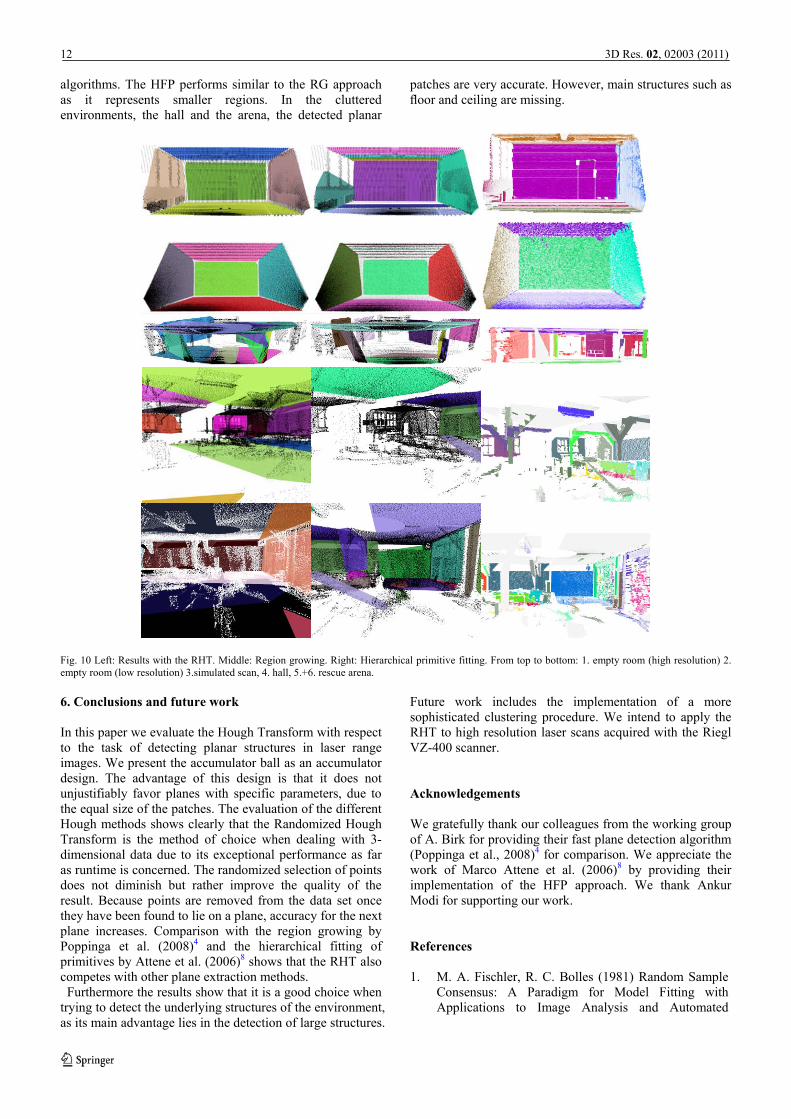
Three times measurements are listed for each data set and method. First, the runtime for the voting phase of the RHT and region growing respectively, second, the time for clustering and calculating the convex hull, and third, the sum of both parts. Additionally, the number of planes found by the algorithms is listed. For the mesh segmentation only the entire runtime is given. Comparison of the runtimes shows the competitiveness of the RHT. The mesh segmentation performs the worst but the runtimes need to be considered with care as a complete hierarchy of planes is generated. For data sets that consist mainly of planes (rows 1 to 3) the RHT outperforms the RG. The runtime of the RHT grows mainly with the number of planes and the number of non-planar points in the data, while the runtime of RG grows with the number of points. This is shown through the runtimes in the forth and fifth row. However, the runtimes remain in a considerable range. The scans with the found planes are shown in Fig. 10. All

algorithms succeed in finding planar structures. From the experiments it appears that the RHT performs better in finding large planes while RG and HFP find planes accurately but tend to detecting several smaller planes rather than one large plane where errors are present in the data. This becomes obvious when looking at the ceiling of the empty room or the simulated scan. RHT nicely fits one plane through the ceiling while RG finds several smaller slices. The same is true for the arena. While the outlines of the building are nicely found by the RHT, RG finds smaller planes within the building that are completely ignored by the RHT. For the HFP the N best planes are depicted, where N is the larger number of planes detected by the other two

12 3D Res. 02, 02003 (2011)

algorithms. The HFP performs similar to the RG approach as it represents smaller regions. In the cluttered environments, the hall and the arena, the detected planar

patches are very accurate. However, main structures such as floor and ceiling are missing.

Fig. 10 Left: Results with the RHT. Middle: Region growing. Right: Hierarchical primitive fitting. From top to bottom: 1. empty room (high resolution) 2. empty room (low resolution) 3.simulated scan, 4. hall, 5.+6. rescue arena. 6. Conclusions and future work In this paper we evaluate the Hough Transform with respect to the task of detecting planar structures in laser range images. We present the accumulator ball as an accumulator design. The advantage of this design is that it does not unjustifiably favor planes with specific parameters, due to the equal size of the patches. The evaluation of the different Hough methods shows clearly that the Randomized Hough Transform is the method of choice when dealing with 3-dimensional data due to its exceptional performance as far as runtime is concerned. The randomized selection of points does not diminish but rather improve the quality of the result. Because points are removed from the data set once they have been found to lie on a plane, accuracy for the next plane increases. Comparison with the region growing by Poppinga et al. (2008)4 and the hierarchical fitting of primitives by Attene et al. (2006)8 shows that the RHT also competes with other plane extraction methods. Furthermore the results show that it is a good choice when

trying to detect the underlying structures of the environment, as its main advantage lies in the detection of large structures.

Future work includes the implementation of a more sophisticated clustering procedure. We intend to apply the RHT to high resolution laser scans acquired with the Riegl VZ-400 scanner. Acknowledgements We gratefully thank our colleagues from the working group of A. Birk for providing their fast plane detection algorithm (Poppinga et al., 2008)4 for comparison. We appreciate the work of Marco Attene et al. (2006)8 by providing their implementation of the HFP approach. We thank Ankur Modi for supporting our work. References 1. M. A. Fischler, R. C. Bolles (1981) Random Sample

Consensus: A Paradigm for Model Fitting with Applications to Image Analysis and Automated

3D Res. 02, 02003 (2011) 13

Cartography, Communications of the ACM. 24:381– 395

2. R. Schnabel, R. Wahl, R. Klein (2007) Efficient RANSAC for Point-Cloud Shape Detection, Computer Graphics Forum.

3. U. Bauer, K. Polthier (2008) Detection of Planar Regions in Volume Data for Topology Optimization, Lecture Notes in Computer Science.

4. J. Poppinga, N. Vaskevicius, A. Birk, K. Pathak (2008) Fast Plane Detection and Polygonalization in noisy 3D Range Images, In IROS ‘08.

5. R. Lakaemper, L. J. Latecki (2006) Extended EM for Planar Approximation of 3D Data, In IEEE International Conference on Robotics and Automation (ICRA ‘06).

6. O. Wulf, K. O. Arras, H. I. Christensen, B. A. Wagner (2004) 2D Mapping of Cluttered Indoor.

7. G. Yu, M. Grossberg, G. Wolberg, I. Stamos (2008) Think Globally, Cluster Locally: A Unified Framework for Range Segmentation, In Proceedings of the 4th International Symposium on 3D Data Processing, Visualization and Transmission (3DPVT ’08), Atlanta, USA.

8. M. Attene, B. Falcidieno, M. Spagnuolo (2006) Hierarchical mesh segmentation based on fitting primitives, The Visual Computer. 22:181–193

9. P. V. C. Hough (1962) Method and Means for Recognizing Complex Patterns, US Patent 3069654.

10. R. O. Duda, P. E. Hart (1971) Use of the Hough Transformation to Detect Lines and Curves in Pictures, Technical Note 36, Artificial Intelligence Center, SRI International.

11. N. Kiryati, Y. Eldar, A. M. Bruckstein (1991) A Probabilistic Hough Transform, Pattern Recognition. 24(4):303–316

12. J. Illingworth, J. Kittler (1988) A Survey on the Hough Transform, Computer Vision, Graphics, and Image Processing. 44:87–116

13. H. Kälviäinen, P. Hirvonen, L. Xu, E. Oja (1995) Probabilistic and Non-Probabilistic Hough Transforms: Overview and Comparisons, Image and Vision Computing. 13(4)

14. A. Ylä-Jääski, N. Kiryati (1994) Adaptive Termination of Voting in the Probabilistic Circular Hough Transform, IEEE Transactions on Pattern Analysis and Machine Intelligence. 16(9)

15. J. Matas, C. Galambos, J. Kittler (1998) Progressive Probabilistic Hough Transform, In Proceedings of the British Machine Vision Conference. 1:256–265

16. L. Xu, E. Oja, P. Kultanen (1990) A new Curve DetectionMethod: Randomized Hough Transform (RHT), Pattern Recognition Letters. 11:331–338

17. A. Censi, S. Carpin (2009) HSM3D: Feature-Less Global 6DOF Scan-Matching in the Hough/Radon Domain, In Proceedings of the IEEE International Conference on Robotics and Automation.

18. T. Zaharia, F. Preteux (2002) Shape-based Retrieval of 3D Mesh Models, In Proceedings of the IEEE International Conference on Multimedia and Expo.

19. D. Borrmann, J. Elseberg (2009) Deforming Scans for Improving the Map Quality Using Plane Extraction and Thin Plate Splines, Master thesis, University of Osnabrück, Germany.

20. F. Tarsha-Kurdi, T. Landes, P. Grussenmeyer (2007) Hough-transform and extended RANSAC algorithms for automatic detection of 3d building roof planes from lidar data, IAPRS. 36:Part 3 / W52

21. M. B. Dillencourt, H. Samet, T. Tamminen (1992) A general approach to connected-component labeling for arbitrary image representations, J. ACM. 39:253–280

22. Environments by Means of 3D Perception, In Proceedings of the IEEE International Conference on Robotics and Automation (ICRA ’04). New Orleans, USA. 4204–4209