The 3-Equation New Keynesian Model — a Graphical

Exposition

Wendy Carlin and David Soskice

University College London and CEPR

Duke University, LSE and Wissenschaftszentrum Berlin

February 2005

Abstract

We develop a graphical 3-equation New Keynesian model for macroeconomic analysis to replace

the traditional IS-LM-AS model. The new graphical IS-PC-MR model is a simple version of the

one commonly used in central banks and captures the forward-looking thinking engaged in by the

policy maker. We show how it can be modified to include a forward-looking IS curve and how

it relates to current debates in monetary macroeconomics, including the New Keynesian Phillips

Curve and the Sticky Information Phillips Curve models.

1 Introduction1

Much of modern macroeconomics is inaccessible to the non-specialist. There is a gulf between the

simple models found in principles and intermediate macro textbooks — notably, the IS-LM -ASapproach — and the models currently at the heart of the debates in monetary macroeconomics in

academic and central bank circles that are taught in graduate courses. Our aim is to show how a

graphical approach can help bridge this divide.

Modern monetary macroeconomics is based on what is increasingly known as the 3-equation

New Keynesian model: IS curve, Phillips curve and interest rate-based monetary policy rule (IS-

PC-MR). This is the basic analytical structure of Michael Woodford’s book Interest and Prices

published in 2003 and, for example, of the widely cited paper “The New Keynesian Science of

Monetary Policy” by Clarida et al. published in the Journal of Economic Literature in 1999. An

earlier influential paper is Goodfriend and King (1997). These authors are concerned to show

how the equations can be derived from explicit optimizing behaviour on the part of the monetary

authority, price-setters and households in the presence of some nominal imperfections. Moreover,

“[t]his is in fact the approach already taken in many of the econometric models used for policy

simulations within central banks or international institutions” (Woodford, 2003, p.237).

Our contribution — motivated by the objective of making modern macroeconomics accessible

— is to provide a graphical presentation of the 3-equation IS-PC-MR model. The IS diagram

is placed vertically above the Phillips diagram, with the monetary rule shown in the latter along

with the Phillips curves. We believe that our IS-PC-MR graphical analysis is particularly useful

for explaining the optimizing behaviour of the central bank. Users can see and remember readily

where the key relationships come from and are therefore able to vary the assumptions about the

behaviour of the policy-maker or the private sector. In order to use the model, it is necessary to

think about the economics behind the processes of adjustment. One of the reasons IS-LM -ASgot a bad name is that it too frequently became an exercise in mechanical curve-shifting: students

were often unable to explain the economic processes involved in moving from one equilibrium to

another. In the framework presented here, in order to work through the adjustment process, the

student has to engage in the same forward-looking thinking as the policy-maker.

David Romer took some steps toward answering the question of how modern macroeconomics

can be presented to undergraduates in his paper “Keynesian Macroeconomics without the LMCurve” published in the Journal of Economic Perspectives in 2000. His alternative to the standard

IS-LM -AS framework follows earlier work by Taylor (1993) in which instead of the LM curve,

there is an interest rate based monetary policy rule.2 While our approach is a little less simple than

Romer’s, it has the advantage of greater transparency.

In this paper, we focus on the explicit forward-looking optimization behaviour of the central

bank. Monetary policy makers must diagnose the nature of shocks affecting the economy and fore-

cast their impact. In sections 1 and 2, the basic graphical analysis for doing this in the IS-PC-MRmodel is set out. The way that central banks adjust the interest rate in response to current informa-

tion about inflation and output is summarized by a so-called Taylor rule. In section 3, we show how

1We are grateful for the advice and comments of Christopher Allsopp, John Driffill, Andrew Glyn, Matthew Hard-

ing, Campbell Leith, Colin Mayer, Edward Nelson, Terry O’Shaughnessy, Nicholas Rau, Daniel Rogger and David

Vines.2Other presentations of “macroeconomics without the LM” are provided in Allsopp and Vines (2000), Taylor

(2000) and in Walsh (2002).

1

a Taylor rule can be derived graphically. A major pre-occupation in monetary macroeconomics in

the past twenty years has been the design of a policy framework to ensure that policy is “time

consistent”, i.e. that the policy maker will not have an incentive to deviate from the optimal policy

after private sector agents have made commitments based on the assumption that the central bank

will stick to its rule. The logic of the time-inconsistency problem and the associated problem of

inflation bias are illustrated graphically in section 4.

In order to introduce the graphical IS-PC-MR model and demonstrate its versatility, we begin

with a standard IS curve without a forward-looking component and a simple ‘backwards-looking’

Phillips curve. In section 5, we provide a graphical explanation of how forward-looking household

behaviour alters the traditional interpretation of the IS curve by including expected future excess

demand in the IS equation (e.g. McCallum and Nelson, 1999). We show how a forward-looking

IS curve, when combined with a monetary policy rule dampens the response of the economy to

shocks. The discussion of agent optimization in the Phillips curve is postponed to section 6.

While the analysis of central bank and household behaviour is widely accepted, the nature of

the Phillips curve remains the subject of sharp disagreement in the literature. Although there is

strong empirical evidence that inflation is highly persistent, it has proved challenging to provide

an explanation for this consistent with optimizing agents, even in the presence of sticky prices

(see for example, Ball, 1994, Fuhrer and Moore, 1995, Nelson, 1998, and Estrella and Fuhrer,

2002). Walsh summarizes the nature of the inflation persistence that is at issue: “In response

to serially uncorrelated monetary policy shocks (measured by money growth rates or by interest

rate movements), the response of inflation appears to follow a highly serially correlated pattern.”

(2003, p.223). Staiger, Stock and Watson (1997), Mankiw (2001), and Eller and Gordon (2003)

provide overviews of the evidence. There are two main contending theories of the Phillips curve

based on optimizing behaviour, the so-called New Keynesian Phillips curve (Clarida et al., 1999)

where price-setters are constrained by sticky prices, and the Sticky Information Phillips curve

(Mankiw and Reis, 2002) where they are constrained by sticky information. In section 6, the

graphical analysis and some simplified maths is used to explain both. The paper concludes with

a comparison between the base-line IS-PC-MR model and the model when modified either by

the use of a forward-looking IS curve or a rational expectations-based Phillips curve with price or

information stickiness.

2 The IS-PC-MR model

We take as our starting point an economy in which policy-makers are faced with a vertical Phillips

curve in the medium run and by a trade-off between inflation and unemployment in the short run.

In setting out the 3-equation model, we make two ad hoc but empirically based assumptions: the

first relates to the persistence of inflation and the second to the time lags in the reaction of the

economy. At this stage, we simply assume that the inflation process is persistent, in line with a

wealth of empirical evidence. In terms of adjustment lags, we assume that it takes one year for

monetary policy to affect output and a year for a change in output to affect inflation. This accords,

for example, with the view of the Bank of England3:

3Bank of England (1999) The Transmission of Monetary Policy p.9

http://www.bankofengland.co.uk/montrans.pdf

2

The empirical evidence is that on average it takes up to about one year in this and

other industrial economies for the response to a monetary policy change to have its

peak effect on demand and production, and that it takes up to a further year for these

activity changes to have their fullest impact on the inflation rate.

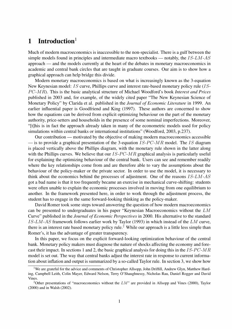
The first step is to present two of the equations of the 3-equation model. The standard IS curve

is shown in the top part of the diagram (Fig.1) as a function of the real interest rate. The real interest

rate is the short-term real interest rate, r. The central bank can set the nominal short-term interest

rate directly, but since the expected rate of inflation is given in the short run, the central bank is

assumed to be able to control r indirectly. In the lower part of the diagram the vertical Phillips

curve at the equilibrium output level, ye, is shown. We think of labour and product markets as

being imperfectly competitive so that the equilibrium output level is where both wage- and price-

setters make no attempt to change the prevailing real wage or relative prices. For convenience, the

‘short-run’ Phillips curves are shown as linear. Each Phillips curve is indexed by the pre-existing

or inertial rate of inflation, πI = π−1. They take the standard simple form in which inflation this

period is equal to lagged inflation plus a term that depends on the difference between the current

level of output and that at which the labour market is in equilibrium, i.e. π = πI + α.(y − ye),where ye is output at the equilibrium rate of unemployment. Given πI , firms faced with excess

demand will be trying to raise relative prices and wage-setters, relative wages.

r

rS

PC(πI=2 )

IS

y

A

A'

π

πT=2

ye

PC(πI=4 )VPC

4

3

1

Figure 1: IS and PC curves

If it is so desired, these Phillips curves can be interpreted as expectations-augmented Phillips

curves in the traditional way where expectations are adaptive. Alternatively, the presence of lagged

3

inflation in the Phillips curve could be the outcome of the imperfect availability of information or

of institutional arrangements in a world where agents have rational expectations. For this reason,

we prefer the more general term of inertial or backwards-looking Phillips curves since the key

assumption relates to the persistence of inflation rather than to a specific expectations hypothesis.

As shown in Fig.1, the economy is in a constant inflation equilibrium at the output level of ye;inflation is constant at the target rate of πT and the real interest rate required to ensure that aggregate

demand is consistent with this level of output is rS , where the ‘S’ stands for the ‘stabilizing’ interest

rate.4

As Romer argues, monetary policy is now usually thought about in terms of a reaction function

that the central bank uses to respond to shocks to the economy and steer it toward an explicit or

implicit inflation target. The first task of the reaction function is to provide a nominal anchor for

the medium run, which is defined in terms of an inflation target. The second task of the reaction

function is to provide guidance as to how the real interest rate should be adjusted in response to

different shocks hitting the economy so that the medium-run objective of stable inflation is met

while minimising output fluctuations. This broad structure for monetary policy can be formalized

as an optimal monetary policy rule in the sense that the monetary rule can be derived as the solution

to the problem faced by the central bank in minimizing the costs of achieving its objectives given

the constraints it faces from the private sector.

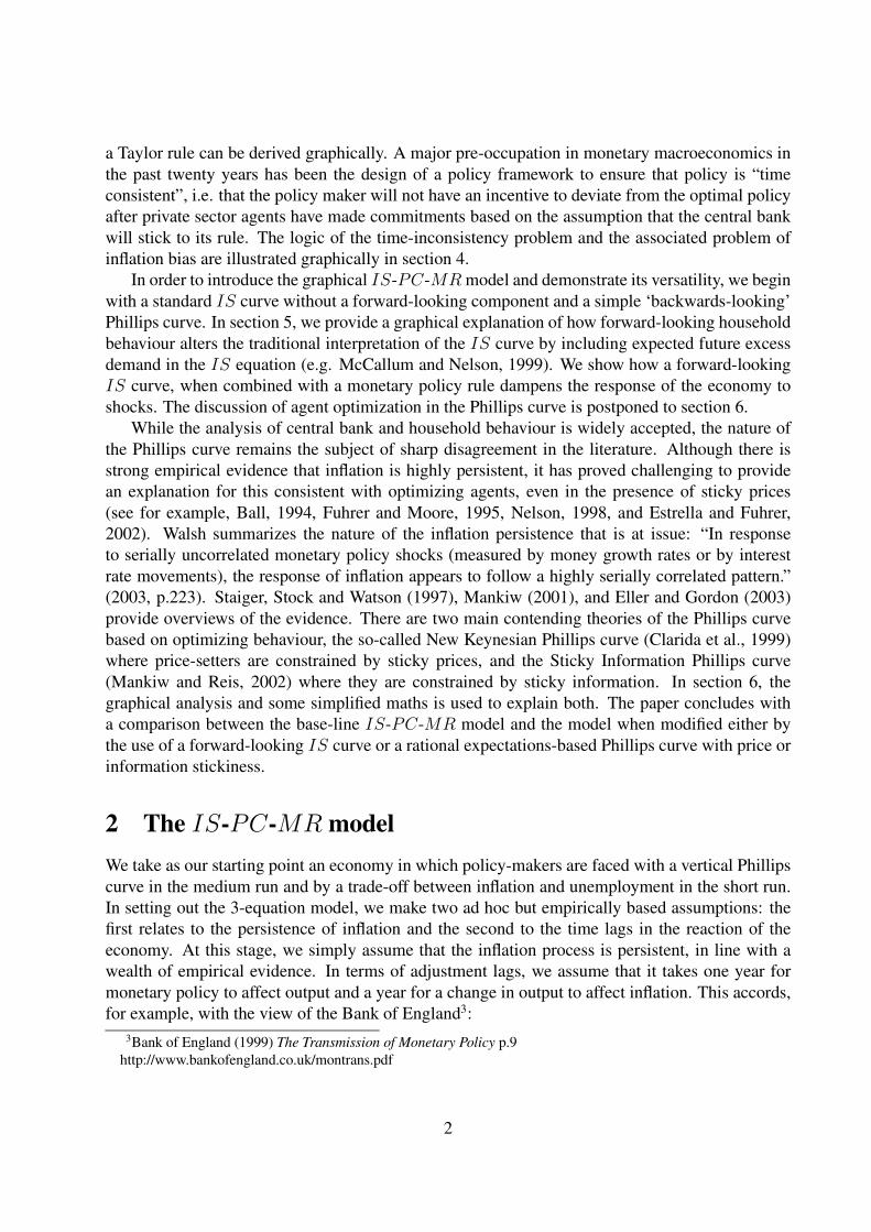
To derive the monetary rule graphically, we need to consider how the central bank behaves. In

Fig.2, we assume that the economy is initially at point B with high but stable inflation (on PC(πI

= 4%)). We assume that the central bank wishes to reduce inflation to its target rate of πT = 2%.

One plausible scenario would be that after a period of higher inflation, a new government is elected,

which charges the central bank with the task of bringing inflation down to the new 2% target rate.

The Phillips curve (PC(πI = 4%)) shows — given last period’s inflation — the feasible inflation

and output pairs faced by the central bank. The only points on the curve with inflation below 4%are to the left of B, i.e. with lower output and hence higher unemployment. With Phillips curves

like this, disinflation will always be costly. This result comes from the assumption that last period’s

inflation always has some influence on inflation this period.

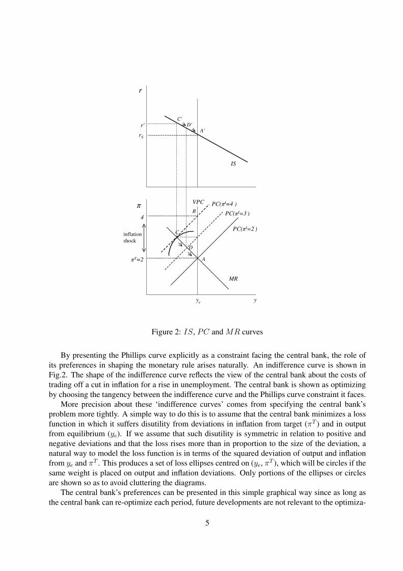
Let us assume that the central bank has chosen to reduce output to point C. In order to do this

by using monetary policy, it must raise the real interest rate to r′. Inflation falls and a new Phillips

curve constraint faces the central bank. The central bank will adjust the interest rate downwards as

inflation falls. The economy moves along the IS curve from C ′ to A′ and along the line labelled

MR for ‘monetary rule’ from C to A. Eventually, the objective of inflation at πT = 2% is achieved

and the economy is at equilibrium unemployment, where it will remain until a new shock or policy

change arises. The MR line shows the level of output the central bank will choose, given the

Phillips curve constraint that it faces. To implement its output choice, the central bank sets the

appropriate interest rate as shown in the IS diagram. As inflation gradually falls, the Phillips

curve shifts down and the central bank chooses an output level closer to the equilibrium: this

traces out the path down the MR along which the economy moves back to equilibrium (i.e. along

the MR from C to D . . . to A in the Phillips diagram; along the IS from C ′ to D′ ... A′ in the ISdiagram).

4Woodford (2003) calls this the Wicksellian or natural rate of interest. We do not follow his usage because rSchanges whenever the IS curve shifts.

4

r

rS

r'

PC(πI=2 )

MR

IS

y

A

B

C

A'

C'D'

π

πT=2

ye

PC(πI=4 )VPC

4PC(πI=3 )

inflation

shock

D

Figure 2: IS, PC and MR curves

By presenting the Phillips curve explicitly as a constraint facing the central bank, the role of

its preferences in shaping the monetary rule arises naturally. An indifference curve is shown in

Fig.2. The shape of the indifference curve reflects the view of the central bank about the costs of

trading off a cut in inflation for a rise in unemployment. The central bank is shown as optimizing

by choosing the tangency between the indifference curve and the Phillips curve constraint it faces.

More precision about these ‘indifference curves’ comes from specifying the central bank’s

problem more tightly. A simple way to do this is to assume that the central bank minimizes a loss

function in which it suffers disutility from deviations in inflation from target (πT ) and in output

from equilibrium (ye). If we assume that such disutility is symmetric in relation to positive and

negative deviations and that the loss rises more than in proportion to the size of the deviation, a

natural way to model the loss function is in terms of the squared deviation of output and inflation

from ye and πT . This produces a set of loss ellipses centred on (ye, πT ), which will be circles if the

same weight is placed on output and inflation deviations. Only portions of the ellipses or circles

are shown so as to avoid cluttering the diagrams.

The central bank’s preferences can be presented in this simple graphical way since as long as

the central bank can re-optimize each period, future developments are not relevant to the optimiza-

5

tion problem. Thus we are implicitly assuming that the central bank has ‘discretion’ to choose the

interest rate each period. This means that it cannot commit to future levels of the interest rate even

though it is concerned about future losses. So although the central bank may currently have a low

inflation target for the future, it cannot bind the hands of future central bank decision-makers to this

target. We return to the discussion of discretion in the context of the problem of time inconsistency

in section 4.

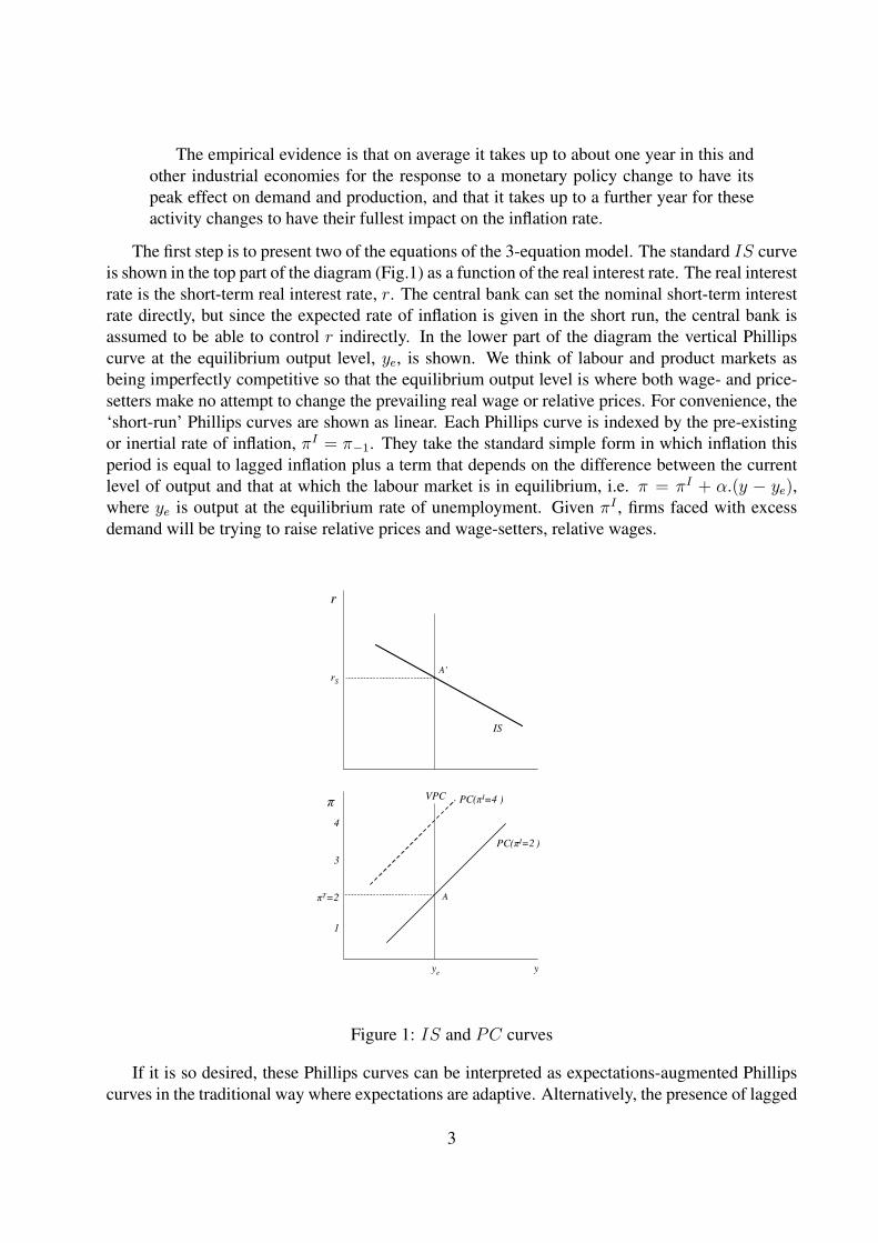
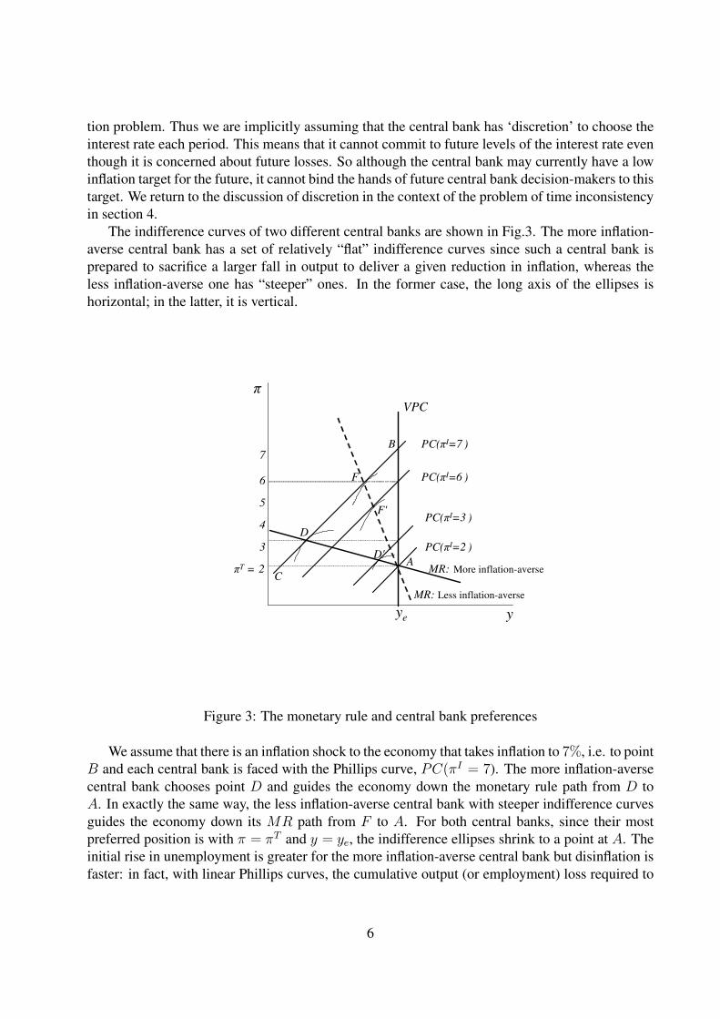
The indifference curves of two different central banks are shown in Fig.3. The more inflation-

averse central bank has a set of relatively “flat” indifference curves since such a central bank is

prepared to sacrifice a larger fall in output to deliver a given reduction in inflation, whereas the

less inflation-averse one has “steeper” ones. In the former case, the long axis of the ellipses is

horizontal; in the latter, it is vertical.

π

y

πT = 2

3

4

ye

A

B

VPC

MR: More inflation-averse

MR: Less inflation-averse

5

6

7

PC(πI=2 )

PC(πI=3 )

PC(πI=6 )

PC(πI=7 )

D'

D

C

F'

F

Figure 3: The monetary rule and central bank preferences

We assume that there is an inflation shock to the economy that takes inflation to 7%, i.e. to point

B and each central bank is faced with the Phillips curve, PC(πI = 7). The more inflation-averse

central bank chooses point D and guides the economy down the monetary rule path from D to

A. In exactly the same way, the less inflation-averse central bank with steeper indifference curves

guides the economy down its MR path from F to A. For both central banks, since their most

preferred position is with π = πT and y = ye, the indifference ellipses shrink to a point at A. The

initial rise in unemployment is greater for the more inflation-averse central bank but disinflation is

faster: in fact, with linear Phillips curves, the cumulative output (or employment) loss required to

6

reduce inflation back to target is independent of the degree of inflation-aversion.5

The MR-curve is shown in the Phillips rather than in the IS-diagram because the essence

of the monetary rule is to identify the central bank’s best policy response to any shock. Both

the central bank’s preferences between output and inflation deviations and the objective trade-off

between output and inflation appear in the Phillips diagram. Moreover, by working in the Phillips

diagram, the impact on the monetary rule of the structure of the supply side, which determines both

the position of the vertical Phillips curve and the slope of the inertia-augmented Phillips curves is

kept to the forefront. Once the central bank has calculated its desired output response by using the

relevant Phillips curve and indifference curve, it is straightforward to go to the IS-diagram and

discover what interest rate must be set in order to achieve this output level. For completeness, it is

important to note that the LM curve depicting the interest rate-output combinations at which the

demand for and supply of money are equal has not literally disappeared from the model. We can

think of there being a ‘shadow’ LM curve that needs to intersect the IS curve at the interest rate

chosen by the central bank in order for that interest rate to be sustained. The use of an interest-rate

based monetary policy rule implies that shocks to the demand for money will be automatically

offset by the central bank in order to maintain its interest rate at target.

Romer (2000), Taylor (2000), Allsopp and Vines (2000) and Walsh (2002) combine the

IS and the MR into a single ‘aggregate demand-inflation curve’ in the Phillips diagram. There

are three reasons why we prefer to show the IS explicitly and thereby provide a direct graphical

correspondence with the 3-equation model. First it reveals a key element of structure by allowing

aggregate demand shocks to be clearly identified as ‘IS shocks’. It is possible to see directly

whether a particular kind of shock requires a change in the interest rate relative to the stabilizing

interest rate, in the stabilizing interest rate only, or in both. Second, it separates the steps in

the central bank’s decision process: what is the optimal output response to any shock given its

preferences and the constraints it faces; how is it be achieved? Finally, as we have seen above, by

keeping the monetary rule separate from the IS, the MR only shifts when there is a change in the

inflation target or in the output target, and its slope reflects only the inputs to the central bank’s

monetary policy decision, i.e. the slope of the Phillips curve and the central bank’s preferences.

3 Aggregate demand and supply shocks

We have already seen how an inflation shock is handled in the IS-PC-MR framework. We now

look briefly at aggregate demand and supply shocks to illustrate the roles played in the transmission

of these shocks by inflation inertia and by lags. It is assumed that the economy starts off with output

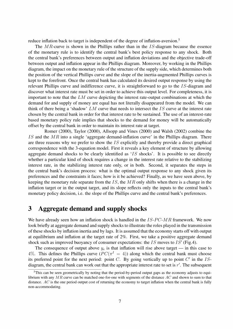
at equilibrium and inflation at the target rate of 2%. First, we take a positive aggregate demand

shock such as improved buoyancy of consumer expectations: the IS moves to IS ′ (Fig.4).

The consequence of output above ye is that inflation will rise above target — in this case to

4%. This defines the Phillips curve (PC(πI = 4)) along which the central bank must choose

its preferred point for the next period: point C. By going vertically up to point C ′ in the IS-

diagram, the central bank can work out that the appropriate interest rate to set is r′. The subsequent

5This can be seen geometrically by noting that the period-by-period output gaps as the economy adjusts to equi-

librium with any MR curve can be matched one-for-one with segments of the distance AC and shown to sum to that

distance. AC is the one period output cost of returning the economy to target inflation when the central bank is fully

non-accommodating.

7

r

rS

r'

PC(πI=2 )

MR

IS

y

A, Z

B

C

A'

C'

Z'

π

πT=2

y'ye

PC(πI=4 )VPC

4

rS'

B'

IS'

Figure 4: Aggregate demand shock and the monetary policy rule

adjustment path down the MR-curve to point Z is exactly as described in the case of the inflation

shock.

This example highlights the role of the stabilizing real interest rate, rS: following the shift in

the IS curve, there is a new stabilizing interest rate and in order to reduce inflation, the interest

rate must be raised above the new rS , i.e. to r′. If the demand shock is only temporary, the IScurve shifts to IS ′ for only one period before returning to its initial position. In this case, there is

no change to the stabilizing interest rate and the central bank simply raises the real interest relative

to the original rS . This example illustrates the importance for the central bank in being able to

forecast the persistence of such shocks.

To summarize, the rise in output builds a rise in inflation above target into the economy. Be-

cause of inflation inertia, this can only be eliminated by pushing output below and (unemployment

above) the equilibrium. The graphical presentation emphasizes that the central bank raises the in-

terest rate in response to the aggregate demand shock because it can work out the consequences

for inflation. The central bank is forward-looking and takes all available information into account:

its ability to control the economy is limited by the presence of inflation inertia and by the time lag

for a change in the interest rate to take effect. When using the model, each of these key elements

8

is encountered as the nature of the shock is diagnosed, its implications for the future worked out

and the central bank’s optimal response deduced.

An aggregate demand shock can be fully offset by the central bank even if there is inflation

inertia if the central bank’s interest rate decision has an immediate effect on output. The economy

then remains at A in the Phillips diagram in which points A and Z coincide and goes directly from

A′ to Z ′ in the IS-diagram. This highlights the crucial role of lags and hence of forecasting for the

central bank: the more timely and accurate are forecasts of shifts in aggregate demand, the greater

is the chance that the central bank can offset such shocks and prevent the impact of inflation from

being built into the economy.

One of the key tasks of a basic macroeconomic model is to help illuminate how the main

variables are correlated following different kinds of shocks. We can appraise the usefulness of the

IS-PC-MR model in this respect by looking at a positive aggregate supply shock and comparing

the optimal response of the central bank and hence the output and inflation correlations with those

above. A supply shock results in a change in the equilibrium rate of unemployment and therefore

a shift in the vertical Phillips curve. It can arise from changes that affect wage- or price-setting

behaviour such as a structural change in wage-setting arrangements, a change in taxation or in

unemployment benefits or in the strength of product market competition, which alters the mark-

up.

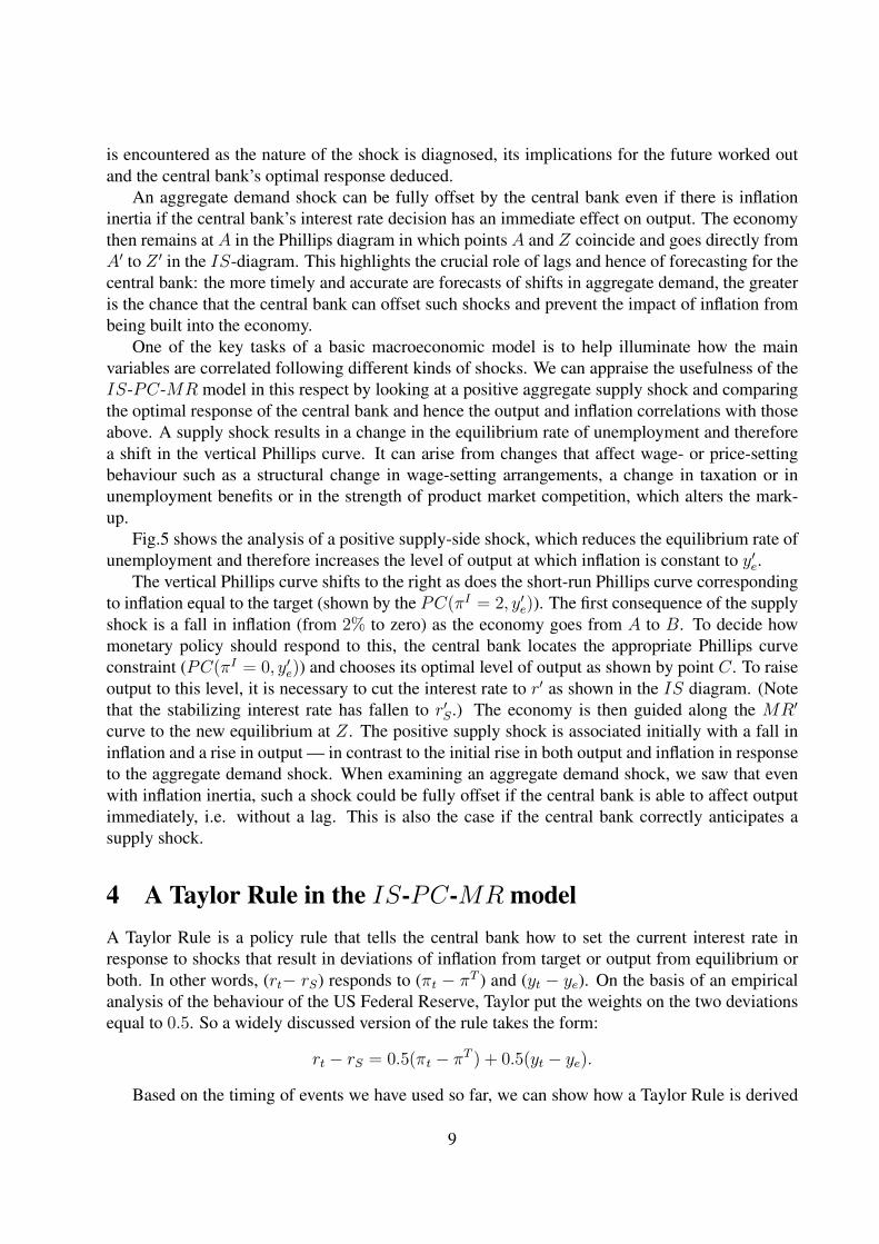
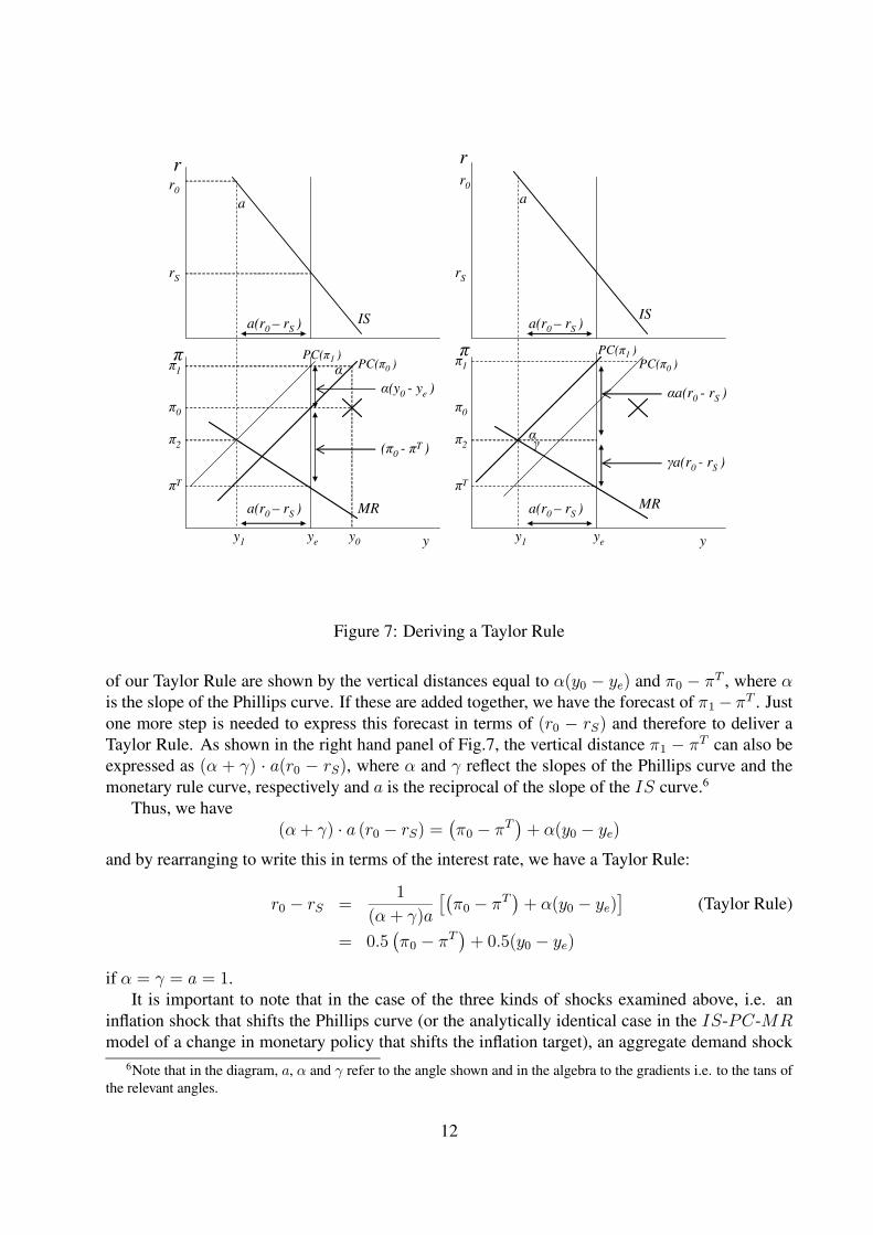
Fig.5 shows the analysis of a positive supply-side shock, which reduces the equilibrium rate of

unemployment and therefore increases the level of output at which inflation is constant to y′e.The vertical Phillips curve shifts to the right as does the short-run Phillips curve corresponding

to inflation equal to the target (shown by the PC(πI = 2, y′e)). The first consequence of the supply

shock is a fall in inflation (from 2% to zero) as the economy goes from A to B. To decide how

monetary policy should respond to this, the central bank locates the appropriate Phillips curve

constraint (PC(πI = 0, y′e)) and chooses its optimal level of output as shown by point C. To raise

output to this level, it is necessary to cut the interest rate to r′ as shown in the IS diagram. (Note

that the stabilizing interest rate has fallen to r′S .) The economy is then guided along the MR′

curve to the new equilibrium at Z. The positive supply shock is associated initially with a fall in

inflation and a rise in output — in contrast to the initial rise in both output and inflation in response

to the aggregate demand shock. When examining an aggregate demand shock, we saw that even

with inflation inertia, such a shock could be fully offset if the central bank is able to affect output

immediately, i.e. without a lag. This is also the case if the central bank correctly anticipates a

supply shock.

4 A Taylor Rule in the IS-PC-MR model

A Taylor Rule is a policy rule that tells the central bank how to set the current interest rate in

response to shocks that result in deviations of inflation from target or output from equilibrium or

both. In other words, (rt− rS) responds to (πt − πT ) and (yt − ye). On the basis of an empirical

analysis of the behaviour of the US Federal Reserve, Taylor put the weights on the two deviations

equal to 0.5. So a widely discussed version of the rule takes the form:

rt − rS = 0.5(πt − πT ) + 0.5(yt − ye).

Based on the timing of events we have used so far, we can show how a Taylor Rule is derived

9

ye'

r

rS

r'

PC(πI=2, ye )MR

IS

y

A

B

Z

C

A'

C'Z'

π

πT=2

y'ye

PC(πI=2, ye')

MR'

VPC VPC'

0

PC(πI=0, ye')

rS'

Figure 5: Aggregate supply shock and the monetary rule

10

π 0

π 1

π 2

y 0

y 1

r0

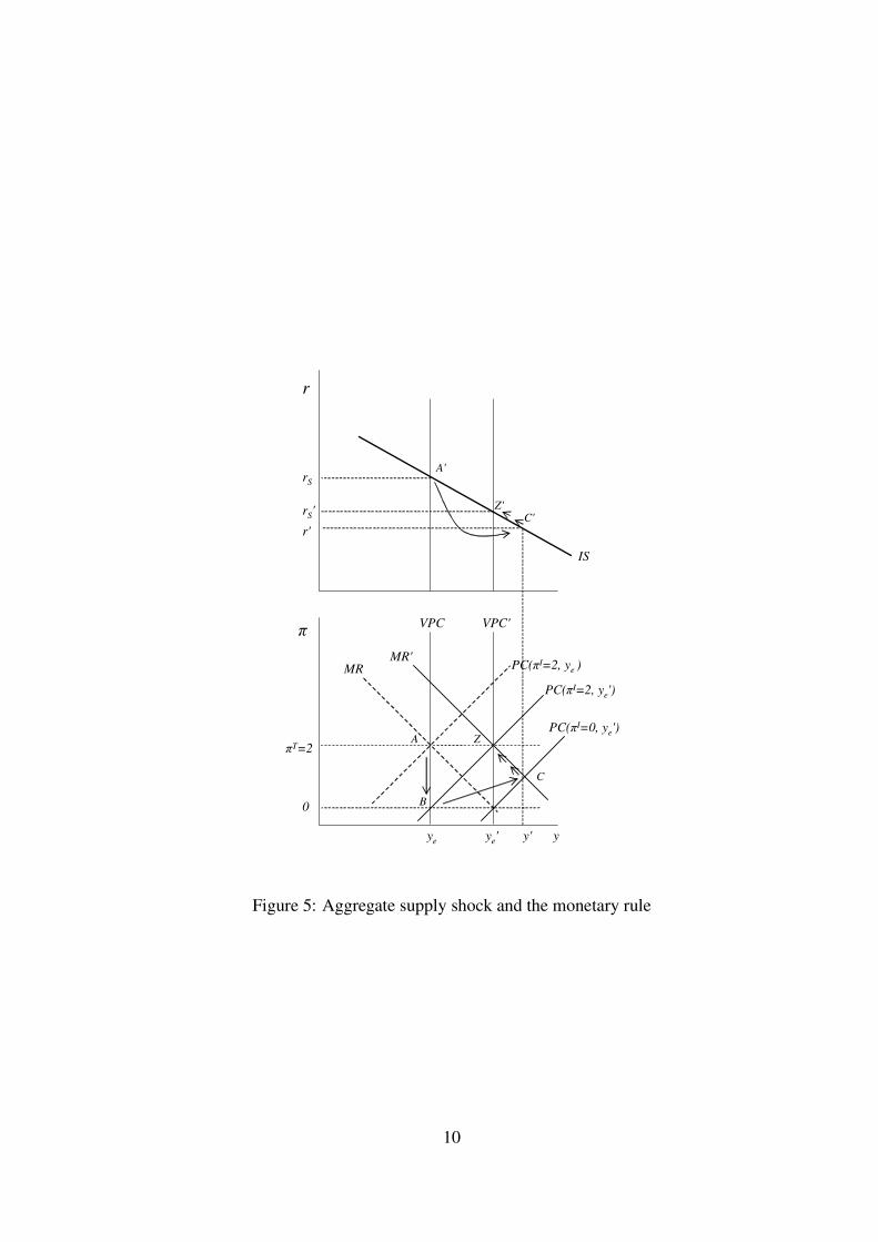
Figure 6: Lag structure in the IS-PC-MR model

geometrically from the IS-PC-MR model. Specifically, we can investigate how the coefficients

on the inflation and output deviations depend on the slopes of the three curves: we shall see that

if the absolute value of the slope of the IS, the Phillips curves and the MR are each equal to one,

then the weights in the Taylor rule are 0.5 and 0.5. This helps bring out the role that differences

in economic structure (demand and supply sides) and in central bank preferences can have on the

coefficients of Taylor Rules.

To see how the central bank should react now to a signal from current economic data about

inflation and output, it is necessary to state clearly the lags between the variables. It is assumed

that there is no observational time lag for the monetary authorities, i.e. the central bank can set

the interest rate (r0) as soon as it observes current data (π0 and y0). However, the interest rate set

now only has an effect on output next period, i.e. r0 affects y1. This is because it takes time for

a change in the interest rate to feed through to consumption and investment decisions. It is also

the case that inflation is affected by output with a lag: i.e. output level y1 affects inflation a period

later, π2. The lag structure is shown in Fig.6 and highlights the fact that a decision taken today

by the central bank to react to a shock will only affect the inflation rate π2. When the economy is

disturbed in the current period (period zero), the central bank looks ahead to the implications for

inflation and sets the interest rate so as to determine y1; which in turn determines the central bank’s

desired value of π2. As the diagram illustrates, action by the central bank in the current period has

no effect on output or inflation in the current period or on inflation in a year’s time.

In Fig.7, the initial observation of output and inflation in period zero is shown by the large

cross, ×. To work out what interest rate to set, the central bank notes that in the following period,

inflation will rise to π1 and output will still be at y0 since a change in the interest rate can only affect

y1. The central bank therefore knows that the constraint it faces is the PC(π1) and it chooses its

best position on it to deliver π2. This means that output must be y1 and therefore that the central

bank sets r0 in response to the initial information shown by point ×. This emphasises that the

central bank is forecasting what inflation will be in period one: its only observed information is

inflation and output at time zero, i.e. point ×.

This reasoning is by now familiar. As shown in the left hand panel of Fig.7, the two components

11

PC(π0 )

r r

π

πT

y

MR MR

π

rS rS

y

r0

IS IS

πT

ye ye

π0 π0

π2 π2

a a

α

α

γ

a(r0 – rS )a(r0 – rS )

a(r0 – rS ) a(r0 – rS )

r0

PC(π0 )PC(π1 )PC(π1 )

π1π1

(π0 - πT )

α(y0 - ye ) αa(r0 - rS )

γa(r0 - rS )

y0y1 y1

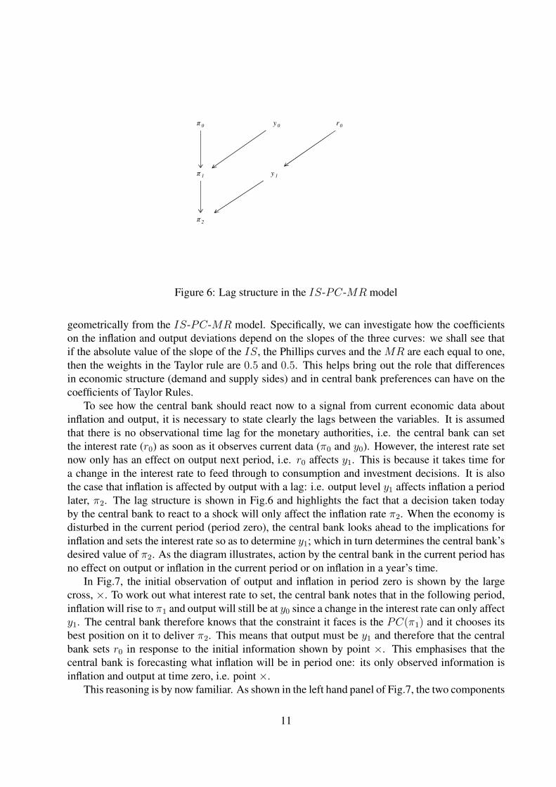
Figure 7: Deriving a Taylor Rule

of our Taylor Rule are shown by the vertical distances equal to α(y0 − ye) and π0 − πT , where αis the slope of the Phillips curve. If these are added together, we have the forecast of π1− πT . Just

one more step is needed to express this forecast in terms of (r0 − rS) and therefore to deliver a

Taylor Rule. As shown in the right hand panel of Fig.7, the vertical distance π1 − πT can also be

expressed as (α + γ) · a(r0 − rS), where α and γ reflect the slopes of the Phillips curve and the

monetary rule curve, respectively and a is the reciprocal of the slope of the IS curve.6

Thus, we have

(α+ γ) · a (r0 − rS) =(π0 − πT

)+ α(y0 − ye)

and by rearranging to write this in terms of the interest rate, we have a Taylor Rule:

r0 − rS =1

(α + γ)a

[(π0 − πT

)+ α(y0 − ye)

](Taylor Rule)

= 0.5(π0 − πT

)+ 0.5(y0 − ye)

if α = γ = a = 1.It is important to note that in the case of the three kinds of shocks examined above, i.e. an

inflation shock that shifts the Phillips curve (or the analytically identical case in the IS-PC-MRmodel of a change in monetary policy that shifts the inflation target), an aggregate demand shock

6Note that in the diagram, a, α and γ refer to the angle shown and in the algebra to the gradients i.e. to the tans of

the relevant angles.

12

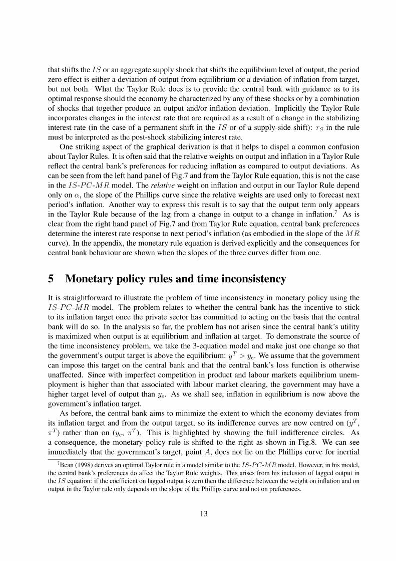
that shifts the IS or an aggregate supply shock that shifts the equilibrium level of output, the period

zero effect is either a deviation of output from equilibrium or a deviation of inflation from target,

but not both. What the Taylor Rule does is to provide the central bank with guidance as to its

optimal response should the economy be characterized by any of these shocks or by a combination

of shocks that together produce an output and/or inflation deviation. Implicitly the Taylor Rule

incorporates changes in the interest rate that are required as a result of a change in the stabilizing

interest rate (in the case of a permanent shift in the IS or of a supply-side shift): rS in the rule

must be interpreted as the post-shock stabilizing interest rate.

One striking aspect of the graphical derivation is that it helps to dispel a common confusion

about Taylor Rules. It is often said that the relative weights on output and inflation in a Taylor Rule

reflect the central bank’s preferences for reducing inflation as compared to output deviations. As

can be seen from the left hand panel of Fig.7 and from the Taylor Rule equation, this is not the case

in the IS-PC-MR model. The relative weight on inflation and output in our Taylor Rule depend

only on α, the slope of the Phillips curve since the relative weights are used only to forecast next

period’s inflation. Another way to express this result is to say that the output term only appears

in the Taylor Rule because of the lag from a change in output to a change in inflation.7 As is

clear from the right hand panel of Fig.7 and from Taylor Rule equation, central bank preferences

determine the interest rate response to next period’s inflation (as embodied in the slope of the MRcurve). In the appendix, the monetary rule equation is derived explicitly and the consequences for

central bank behaviour are shown when the slopes of the three curves differ from one.

5 Monetary policy rules and time inconsistency

It is straightforward to illustrate the problem of time inconsistency in monetary policy using the

IS-PC-MR model. The problem relates to whether the central bank has the incentive to stick

to its inflation target once the private sector has committed to acting on the basis that the central

bank will do so. In the analysis so far, the problem has not arisen since the central bank’s utility

is maximized when output is at equilibrium and inflation at target. To demonstrate the source of

the time inconsistency problem, we take the 3-equation model and make just one change so that

the government’s output target is above the equilibrium: yT > ye. We assume that the government

can impose this target on the central bank and that the central bank’s loss function is otherwise

unaffected. Since with imperfect competition in product and labour markets equilibrium unem-

ployment is higher than that associated with labour market clearing, the government may have a

higher target level of output than ye. As we shall see, inflation in equilibrium is now above the

government’s inflation target.

As before, the central bank aims to minimize the extent to which the economy deviates from

its inflation target and from the output target, so its indifference curves are now centred on (yT ,

πT ) rather than on (ye, πT ). This is highlighted by showing the full indifference circles. As

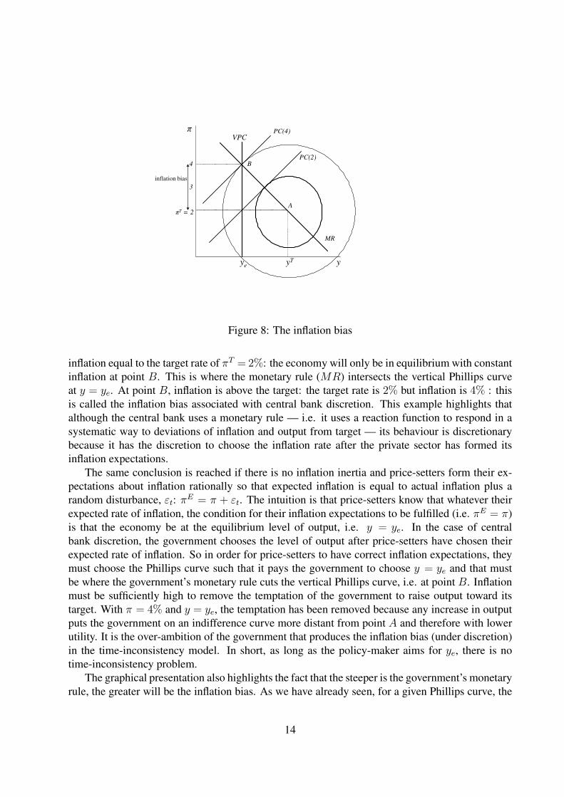
a consequence, the monetary policy rule is shifted to the right as shown in Fig.8. We can see

immediately that the government’s target, point A, does not lie on the Phillips curve for inertial

7Bean (1998) derives an optimal Taylor rule in a model similar to the IS-PC-MRmodel. However, in his model,

the central bank’s preferences do affect the Taylor Rule weights. This arises from his inclusion of lagged output in

the IS equation: if the coefficient on lagged output is zero then the difference between the weight on inflation and on

output in the Taylor rule only depends on the slope of the Phillips curve and not on preferences.

13

π

y

πT = 2

3

4

yTye

PC(2)

PC(4)

A

B

MR

inflation bias

VPC

Figure 8: The inflation bias

inflation equal to the target rate of πT = 2%: the economy will only be in equilibrium with constant

inflation at point B. This is where the monetary rule (MR) intersects the vertical Phillips curve

at y = ye. At point B, inflation is above the target: the target rate is 2% but inflation is 4% : this

is called the inflation bias associated with central bank discretion. This example highlights that

although the central bank uses a monetary rule — i.e. it uses a reaction function to respond in a

systematic way to deviations of inflation and output from target — its behaviour is discretionary

because it has the discretion to choose the inflation rate after the private sector has formed its

inflation expectations.

The same conclusion is reached if there is no inflation inertia and price-setters form their ex-

pectations about inflation rationally so that expected inflation is equal to actual inflation plus a

random disturbance, εt: πE = π + εt. The intuition is that price-setters know that whatever their

expected rate of inflation, the condition for their inflation expectations to be fulfilled (i.e. πE = π)

is that the economy be at the equilibrium level of output, i.e. y = ye. In the case of central

bank discretion, the government chooses the level of output after price-setters have chosen their

expected rate of inflation. So in order for price-setters to have correct inflation expectations, they

must choose the Phillips curve such that it pays the government to choose y = ye and that must

be where the government’s monetary rule cuts the vertical Phillips curve, i.e. at point B. Inflation

must be sufficiently high to remove the temptation of the government to raise output toward its

target. With π = 4% and y = ye, the temptation has been removed because any increase in output

puts the government on an indifference curve more distant from point A and therefore with lower

utility. It is the over-ambition of the government that produces the inflation bias (under discretion)

in the time-inconsistency model. In short, as long as the policy-maker aims for ye, there is no

time-inconsistency problem.

The graphical presentation also highlights the fact that the steeper is the government’s monetary

rule, the greater will be the inflation bias. As we have already seen, for a given Phillips curve, the

14

monetary rule is steeper for a less inflation-averse central bank.

6 The forward looking IS curve

In the traditional IS curve, aggregate demand shocks are amplified through the operation of the

multiplier. Once a forward-looking IS curve is introduced, demand shocks are dampened as the

behaviour of households interacts with that of the forward-looking central bank. A typical way of

introducing forward-looking behaviour in the IS curve is to ignore investment and concentrate at-

tention on consumption behaviour. Households are assumed to make their consumption decisions

on the basis of their expected future income in such a way that their life-time utility is maximized.

Since it is assumed that households wish to smooth consumption over time, higher expected future

output, which entails higher future consumption, will raise current consumption and output. A

higher real interest rate depresses consumption because of the household’s ability to substitute fu-

ture for current consumption (it is assumed that the substitution effect outweighs the income effect

of an interest rate change). Government expenditure is incorporated in an exogenous demand term.

The so-called Euler condition for optimal consumption over time is derived from the household’s

optimization problem and when combined with the exogenous demand, At, implies an equation of

the following form for the IS curve8:

yt = Etyt+1 +At − art−1

where Etyt+1 is the expectation formed in period t of the value of output in period t+ 1.The stabilising short term real rate of interest, rS , is defined by ye,t = Etye,t+1 + At − arS,t,

and since some algebra is necessary, we simplify the notation by defining the gap between actual

and equilibrium output as x, ‘excess demand’: xt ≡ yt − ye. The IS equation can be written in

terms of deviations from equilibrium as follows:

xt = Etxt+1 − a (rt−1 − rS,t) . (Forward-looking IS)

In this section, we use the same lag structure as before. We also continue to assume that the Phillips

curve is backwards looking, and that the monetary authority adopts a discretionary optimising

policy:

πt = πt−1 + αxt−1 (Phillips curve)

xt = −1

γ

(Etπt+1 − πT

). (Monetary policy rule)

How is the analysis of inflation and demand shocks affected by the requirement that the au-

thorities take into account the impact of future output on current demand in the IS curve; and

that households work out the effect on future output and hence on their current demand of the

consequences of shocks for the actions of the central bank? We develop our graphical approach

to show that the forward-looking behaviour of households dampens the interest rate consequences

of shocks. The intuition is straightforward: households can forecast that a positive inflation shock

now will lead to increased (though declining) interest rates over future periods until equilibrium

is again restored. Hence households immediately dampen demand by more than the impact of an

8See, for example, McCallum and Nelson (1999) for the details.

15

increased short-term interest rate so as to smooth the effect of the future higher interest rates on

their consumption path.

This can be seen by rewriting the forward-looking IS curve as:

xt = −a (rt−1 − rS,t)− a(rt − rS,t+1)− a (rt+1 − rS,t+2)− ...

In other words, current demand is a function, not just of the lagged real short-term interest rate,

but of all (expected)) future real short term interest rates. Thus household demand immediately

contracts in response to the full course of expected future real interest rates. This means in turn

that the central bank — so long as it works through the implications of forward looking household

behaviour — needs to raise interest rates by less than it otherwise would to achieve the desired re-

duction in inflation. The anticipatory behaviour of households and the central bank are reinforcing,

so that output falls and interest rates rise less than in our previous examples (with the traditional

IS curve). We illustrate the difference that the forward-looking IS curve makes by looking at an

inflation shock (the case of an IS shock is shown in the appendix).

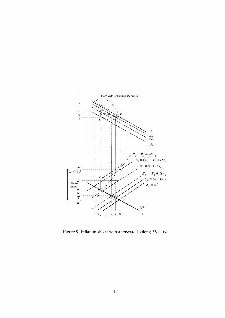
We start in equilibrium (in Fig.9) with π−1 = πT and x−1 = 0 (at point A). In period zero there

is an inflation shock of ε, so that

π0 =(πT + ε

)+ αx−1 = πT + ε.

The economy moves up the vertical Phillips Curve to π0 = πT + ǫ at point B. What happens to

excess demand in period zero? As usual, the central bank cannot influence this directly since the

effect of its interest rate decision takes effect with a lag. Hence the interest rate that affects output

in period zero is r−1 = rS . However, the central bank can affect current period output indirectly:

the IS equation at period zero says that x0 = E0x1 − a (r−1 − rS) = x1. From now on we drop

the expectations operator. As we shall see, since households at time zero can work out that the

central bank will choose to raise r0 in order to create x1 < 0, households will immediately cut

back demand in period zero in anticipation of this.

How precisely do households form expectations of x1? Since the central bank can only in-

fluence inflation in period two and output in period one, households know that the central bank

chooses the pair jointly at the intersection of the monetary rule line, MR and the period two

Phillips curve, π2 = π1 + αx1. But in order to know π1 the central bank has to work out x0,because π1 = π0 + αx0. Since households will set x0 = x1, the central bank can work out the

period two Phillips curve as:

π2 = π1 + αx1 = (π0 + αx0) + αx1 = π0 + 2αx1.

This is the steeper Phillips curve shown by the dashed line in Fig.9. Thus households can in

turn forecast that the central bank’s choice of (π2, x1) will be at the intersection of the MR and

π2 = π0 + αx1 (point D). It can also be shown that

x0 = x1 = −γε

1 + 2αγ.

Now Fig.9 can be used to see what happens in periods zero and one. In period zero, households

cut demand to x0. We know where that is in the diagram since it is equal to x1. Since π1 = π0+αx0,π1 also falls; we move from point B to point C in the Phillips curve diagram.

16

0(T

xπ π ε α1 = + ) +

2 1 1xπ π α= +

3 2 2xπ π α= +

4 3 3xπ π α= +

2π

1π

3π

4π

0π

Tπ

Tπ ε= +

x0=x1 x2 x3 0

r

rS

r0r1

r*

2 0 12 xπ π α= +

x*

π-1= πT

MR

inflation

shock

IS1

IS-1

IS0

IS2

x

Path with standard IS curve

A

B

D

C

A'

C'

D'

Figure 9: Inflation shock with a forward-looking IS curve

17

The future path of excess demand and inflation, (π3, x2) , (π4, x3) , ... is easy to work out. This

is because each pair is chosen by the central bank in the relevant time period by the intersection

of the MR line with the relevant Phillips curve. So (π3, x2), is the intersection of MR with the

PC, π3 = π2 + αx2, and so on. Thus once the economy has reached (π2, x1) i.e. point D, the

adjustment path down the MR line is the same as in the analysis in section 1.

We now turn to the path of interest rates, and to the IS diagram. Given the time lags between

a change in the interest rate and its effect on the output gap and of the output gap to inflation, the

central bank chooses r0 to set (π2, x1) (point D′), r1 to set (π3, x2), r2 to set (π4, x3), etc. The

initial IS curve, IS−1, goes through the vertical Phillips curve at rS . This is because E−1x0 = 0,so that x−1 = E−1x0 − a (r−2 − rS) = −a (r−2 − rS); and since r−2 = rS, x−1 = 0. In period

zero, the IS curve, IS0, is given by

x0 = E0x1 − a (r−1 − rS) .

It is easy to see that this IS curve at time zero goes through the intersection of x1 and rS (point

C ′). Since r−1 = rS , this confirms that x0 = x1. In other words, the anticipation by the household

of the central bank’s action leads it to reduce consumption before the interest rate rises. The IScurve in period 1, IS1, is

x1 = E1x2 − a (r0 − rS) ,

and goes through rS at x2. Hence to ensure that the central bank can hit its x1 target, it needs to set

r0 above r−1, where x2 intersects IS1. In the same way, IS2

x2 = E2x3 − a (r1 − rS)

intersects rS at x3. And r1 is given by the intersection of IS2 with x3. And so on.

Thus, it can be seen, that less excess supply and correspondingly lower interest rates are needed

by the central bank to adjust back to equilibrium after an inflation shock with a forward looking

IS curve. With an ordinary IS curve, households do not take into account the future pattern of

deflation the central bank will impose in the event of a shock of this kind. Therefore the central

bank has to impose a bigger recession. With such an IS curve, x0 = 0 since households take no

account of the fact that x1 will be negative. Hence the period two Phillips curve is π2 = π0 + αx1and the pair (π2, x1) is determined by the intersection of the monetary rule line with this Phillips

curve with x1 = x∗. Moreover, since there is a unique IS curve (which goes through the vertical

Phillips curve at rS), r0 = r∗ is at the intersection of that IS curve and x1 = x∗. The adjustment

process in the IS diagram is shown by the dashed line in Fig.9. The outcome is that cycles are

more muted as the forward-looking behaviour of households and the central bank reinforce each

other.

7 Debates over Phillips curves: the New Keynesian Phillips

Curve versus the Sticky Information Phillips Curve

The IS-PC-MR model provides a simple macro-economic framework for use in analyzing con-

temporary performance and policy issues. It matches the empirical evidence concerning inflation

persistence and the lag structure of key variables. Its main shortcoming is that it rests on ad hoc

18

assumptions — in particular about the inflation process — rather than being derived from an opti-

mizing micro model of firm behaviour. An important manifestation of this problem relates to the

issue of the credibility of monetary policy. We have seen in section 1 that when the central bank an-

nounces a lower inflation target, the economy moves only slowly towards this as the Phillips curve

shifts period-by-period (as shown in Fig.2). Whether or not the central bank’s announcement is

believed by the private sector makes no difference at all to the path of inflation. For this reason, the

analysis of an inflation shock and of an announced change in the inflation target is identical in the

IS-PC-MR model: either way, the inflation that is built into the system takes time (with higher

unemployment) to work its way out. The inability of the model to take into account the reaction

of price-setters to announced changes in monetary policy is unsatisfactory. Recent developments

in modelling the Phillips curve aim to provide a micro-optimizing based model that can produce

both costly disinflation and a role for the credibility of monetary policy.

7.1 The New Keynesian Phillips Curve

The New Keynesian Phillips Curve (NKPC) is derived from the Calvo model (1983), which com-

bines staggered price-setting by imperfectly competitive firms and the use of rational expectations

by private sector agents. Specifically, Calvo assumes that each period a proportion δ of firms, ran-

domly chosen, can reset their prices. Using this assumption, Clarida et al. (1999) show that the

Phillips curve — the so-called New Keynesian Phillips curve — then takes a particularly simple

form in which inflation depends on the current gap between actual and equilibrium output as in the

standard Phillips curve but on expected future inflation rather than on past inflation. The NKPCtakes the following form:

πt =αδ

1− δxt + θEtπt+1 (NKPC)

where θ is the discount factor (θ < 1) and Etπt+1 is the expected value of inflation in t + 1 at t.In an appendix we provide a simplified explanation of how the NKPC is derived from the sticky

price assumption. The larger the per cent of firms that can set their price in the current period, the

more important is current excess demand as a determinant of inflation, shown by the term δ/(1−δ).The intuition is that current excess demand will be more important than future factors if there is a

high chance you can reset your price each period. In terms of the graphical presentation, a higher

presence of price-stickiness, i.e. lower δ, implies a flatter Phillips curve; if all firms set prices every

period, δ = 1 and the Phillips curve is vertical.9 This is of course the case of rational expectations

with full price flexibility.

The most important point about the NKPC equation is that current inflation depends simply:

(i) on the present, i.e. on the current output gap, xt, and (ii) on the future, embodied in Etπt+1.There is no role for last period’s inflation, despite sticky prices. The big advantage of the NKPCis that it embodies rational expectations on the part of all agents.

In order to use the NKPC, it is necessary to work out how rational agents form their expecta-

tions of future inflation, Etπt+1. To do this, we need to derive the monetary rule. This is done as

before by minimizing the central bank’s loss function subject to the Phillips curve, in this case, the

9As is clear from the equation, the NKPC delivers a non-vertical long-run Phillips curve because of the presence

of the discount factor, θ. This feature of the NKPC is unsatisfactory but we do not pursue it here. Since θ will be

close to 1, we show it as vertical in the figures.

19

NKPC. As shown in the appendix, this produces the usual monetary rule, which can be written

as:

πt = −γxt, (MR)

where γ = 1−δδαβ

and reflects the slope of the Phillips curve and the inflation-aversion of the central

bank as in the IS-PC-MR model as well as the “Calvo coefficient”, δ. The intuition is that both

the NKPC and the monetary rule have to hold in each period and this implies that expected

inflation is equal to the central bank’s inflation target (for the details, see the appendix). This result

is neat and has the attractive property that the credibility of monetary policy matters. In terms of

the IS-PC-MR diagram, the NKPC always intersects the MR schedule at (y = ye and π =πT ), in the absence of unanticipated shocks. Thus an announced reduction in the inflation target

would immediately translate into an equivalent reduction in inflation since the NKPC would jump

to its new position and output would remain unchanged. Inflation depends on future expected

inflation and this changes as soon as a new inflation target is announced. Although only δ% of

firms can change their prices, they alter them taking into account their rational expectation of

when they will next be able to optimize and this calculation leads to aggregate inflation jumping

to the new inflation target. The NKPC has the property that credibility matters but brings with it

the disadvantage that there is no inflation persistence and therefore no output cost associated with

a change in monetary policy.

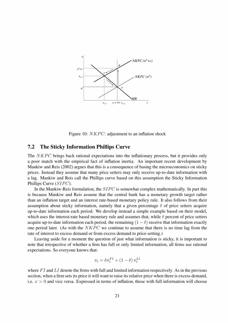
Let us check whether the NKPC meets the requirement that an unanticipated one-period

inflation shock, such as a cost shock, entails a costly disinflation. Such a shock shifts the NKPCvertically upwards as shown in Fig.10 by the NKPC(πT + ǫ). The δ proportion of firms that can

reset their prices take this into account and optimize whilst the prices of the other 1−δ firms remain

as determined by their previous pricing decision. Since the latter group cannot change their pricing

decision, they react by cutting output by more than do the price-setters. The aggregate result for the

economy is shown by the intersection of the MR curve and the NKPC curve at point C in Fig.10.

Hence the consequence of the inflation shock is a reduction in activity in the economy below the

equilibrium. The next period, however, the economy will once again be at equilibrium with target

inflation (point A): the cost shock has gone and the inflation outcome the previous period has

no lasting effect on either group of price-setters. It is also important to note that a higher degree

of price-stickiness is reflected purely in the magnitude of the one-period unemployment cost of

disinflation (a higher weight of stickiness means the NKPC and MR are both flatter and hence

the one-period fall in output is higher).

The inability of the NKPC to account for the persistence of inflation following a shock is

its Achilles heel: there is no inflation persistence following a change in monetary policy and only

a single period impact on inflation following an inflation shock (using Fig.10, if the economy

is initially in equilibrium at point B, it goes straight to point A following an announced reduc-

tion in the inflation target to πT ). Clarida et al. attempt to build more realistic results into their

model by introducing an exogenous “cost push” factor, c, which is an inflation shock, the effect

of which is assumed to diminish over time. The mechanics of the NKPC with such an autocor-

related cost-push shock added are set out in the appendix. By assumption, this modified model

produces inflation inertia, with disinflation taking place over many periods, but in common with

the backwards-looking Phillips curve, it lacks micro-foundations.

20

MRxt = 0= xt+2 xt+1

NKPC (πT)

x

NKPC (πT+ε)

π

πt+1

πT+ε

πT A

B

C

Figure 10: NKPC: adjustment to an inflation shock

7.2 The Sticky Information Phillips Curve

The NKPC brings back rational expectations into the inflationary process, but it provides only

a poor match with the empirical fact of inflation inertia. An important recent development by

Mankiw and Reis (2002) argues that this is a consequence of basing the microeconomics on sticky

prices. Instead they assume that many price setters may only receive up-to-date information with

a lag. Mankiw and Reis call the Phillips curve based on this assumption the Sticky Information

Phillips Curve (SIPC).

In the Mankiw-Reis formulation, the SIPC is somewhat complex mathematically. In part this

is because Mankiw and Reis assume that the central bank has a monetary growth target rather

than an inflation target and an interest rate-based monetary policy rule. It also follows from their

assumption about sticky information, namely that a given percentage δ of price setters acquire

up-to-date information each period. We develop instead a simple example based on their model,

which uses the interest-rate based monetary rule and assumes that, while δ percent of price setters

acquire up-to-date information each period, the remaining (1− δ) receive that information exactly

one period later. (As with the NKPC we continue to assume that there is no time lag from the

rate of interest to excess demand or from excess demand to price-setting.)

Leaving aside for a moment the question of just what information is sticky, it is important to

note that irrespective of whether a firm has full or only limited information, all firms use rational

expectations. So everyone knows that:

πt = δπFIt + (1− δ) πLIt

where FI and LI denote the firms with full and limited information respectively. As in the previous

section, when a firm sets its price it will want to raise its relative price when there is excess demand,

i.e. x > 0 and vice versa. Expressed in terms of inflation, those with full information will choose

21

the inflation rate

πFIt = πt + αxt

since they are assumed to know or be able to work out πt and xt. And those with limited informa-

tion will set

πLIt = Et−1 (πt + αxt) .

Since all firms use rational expectations, they all know the equation

πt = δ (πt + αxt) + (1− δ) (Et−1πt + αEt−1xt)

=αδ

1− δxt + Et−1πt + αEt−1xt.

Of course those with limited information will not necessarily know πt and xt. However, using

rational expectations the LI firms can deduce

Et−1πt =αδ

1− δEt−1xt + Et−1πt + αEt−1xt,

which implies that Et−1xt = 0.To find out Et−1πt, the LI firms now simply have to use the monetary rule, namely πt =

πt−1 − γxt. This implies Et−1πt = Et−1πTt − γEt−1xt = Et−1π

Tt since Et−1xt = 0. Going back

to the earlier equation for πt, it can now be rewritten as the Sticky Information Phillips Curve

πt =αδ

1− δxt + Et−1π

Tt . (SIPC)

And together with the monetary rule,

πt = πTt − γxt, (MR)

these two equations determine πt and xt. The slope of the SIPC depends on α and on δ, but in

this case unlike the NKPC, δ refers to the proportion of price-setters with up-to-date information.

As δ tends toward one, the Phillips curve becomes vertical: this is the standard case of rational

expectations with flexible prices and full information. If δ < .5, the slope is flatter than α, and vice

versa. We need to highlight the critical difference with the NKPC. In the NKPC,

πt =αδ

1− δxt + θEtπt+1.

In the SIPC, the Etπt+1 term is replaced by Et−1πt. In other words, if wage and price setters

are rational in an NKPC world it is difficult to see how inflation inertia can come about, since

Etπt+1 depends on expectations at t about future inflation. But in a SIPC world the most up to

date information that (1 − δ) percent of firms may have in forming their views about πt at t − 1,i.e. Et−1πt, may plausibly include past factors that influence πt−1.

Let us assume that the limited information relates to the central bank’s inflation target. This

key case for monetary policy allows us to show both that disinflation is costly in the SIPC model

when the central bank lowers its inflation target — in contrast to the NKPC modelling of this case

— and that credibility matters. The model implies that if those with limited information believe

22

MR1

x0 = 0= x2 x1 x

SIPC1,0

π

π1

π0 = π0T

A

B

Cπ2 = π1

T

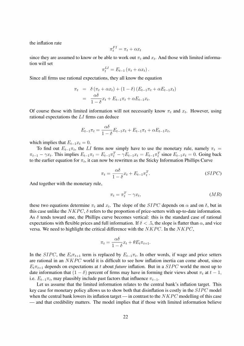
Figure 11: SIPC: Reduction of the inflation target; one period delay in information assimilation

(rightly or wrongly) that the central bank’s target is πT0 , and if the central bank reduces its target to

πT1 in period one, the SIPC at period one is

π1 =αδ

1− δx1 + πT0

and we call this SIPC1,0. As we have seen, it holds as SIPCt,0 for each period t in which those

with limited information think the target is πT0 .

In Fig.11, the initial equilibrium is at (πT0 , x = 0), with π0 = πT0 and x0 = 0 (at point A).

In period one, the central bank reduces the inflation target to πT1 , so that the MR1 goes through

x = 0 and π = πT1 and the SIPC becomes SIPC1,0. Hence excess supply of x1 is created and

inflation falls to π1 > πT1 . In period two all firms have full information and the economy moves to

the (π2 = πT1 , x2) equilibrium at point C.

Two consequences should be noted in this example: disinflation is costly following a change in

monetary policy and once those with limited information have understood that the inflation target

has fallen, they immediately adjust their behaviour. Thus by contrast with the backwards-looking

Phillips curve, the credibility of the central bank’s announcement plays a role in adjustment and

by contrast with the NKPC, there is a cost of disinflation when the inflation target changes.

However, it is not really appropriate to compare the SIPC with a one period delay in infor-

mation assimilation to the NKPC because the NKPC assumes that there is a distribution over

time in the ability of firms to change their price. The appropriate comparison entails allowing in-

formation to diffuse more slowly in the SIPC. When we allow for more than a one-period lag in

information assimilation this has the effect of slowing down the adjustment of the economy back

to equilibrium following a shock, with the result that it is able better to predict the empirically

observed phenomenon of inflation persistence.

To illustrate this we now assume that δ1 per cent of firms acquire immediate knowledge of the

target reduction in the inflation target, δ2 per cent cumulatively after one period, δ3 per cent after

23

0 0

Tπ π=

1π

1x 4x

1,0 1( )SIPC δ

2π

3x2x

3π

2,0 2( )SIPC δ

3,0 3( )SIPC δ

1( )MR δ2( )MR δ

3( )MR δπ4 = π1T

x

π

C

B

A

D

E

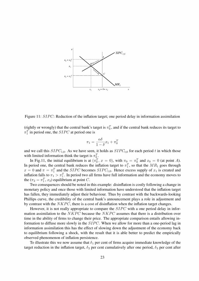
Figure 12: SIPC: Reduction of inflation target; information diffusion over several periods

two periods, and all firms after four periods. The reduction of output and inflation in period one (to

π1, x1) takes place in an identical way to the previous one-lag model with δ = δ1. In period two,

all that happens is that the percentage of firms with full information rises to δ2 and therefore of

limited information falls to (1−δ2), which implies that SIPC2,0(δ2) is given by π2 =αδ21−δ2

x2+πT0 .

This is a steeper curve than SIPC1,0(δ1), as can be seen in Fig.12. Likewise with SIPC3,0(δ3) in

period three.

The monetary rule curve, MR1, also changes with δ. This is because the central bank, faced

with a Phillips curve constraint π = αδ1−δ

x+ πT0 sets an optimal monetary rule under discretion of

(π − πT1 ) = −1−δδαβ

x. Thus, as δ increases (and the PC(δ) gets steeper), MR(δ) gets flatter. It can

be seen that inflation falls as the share of firms with full information, δ, rises; and after δ has risen

sufficiently the output gap will start to rise towards zero. The economy moves from point A to Bto C to D and back to the new equilibrium at E. Hence we get a closer approximation to inflation

inertia.10

However, it could be argued that this assumption of slowly diffusing information is just as ad

hoc as the assumption of an exogenously decaying cost shock in the NKPC. The SIPC model

does not provide an explanation for slow information acquisition in terms of the incentives of

agents.

10It can be shown that, if the actual path of inflation is know ex-post to all firms the inflation they set will cancel out

previous relative price changes.

24

8 Conclusion

The graphical IS-PC-MR model is a replacement for the standard IS-LM -AS model. It con-

forms with the view that monetary policy is conducted by forward-looking central banks and pro-

vides non-specialists with the tools for analyzing a wide range of macroeconomic disturbances. By

building on the lag structure consistent with empirical evidence, the model allows a Taylor Rule to

be derived graphically.

The IS-PC-MR model also provides access to contemporary debates in the more specialized

monetary macroeconomics literature. It is straightforward to demonstrate the origin of the time

inconsistency problem using the graphical approach. The model is extended to show how replacing

the traditional IS curve with an IS incorporating forward-looking behaviour dampens the effect

of shocks on output and inflation.

As demonstrated by the lively debates in the literature and in central banks over recent years,

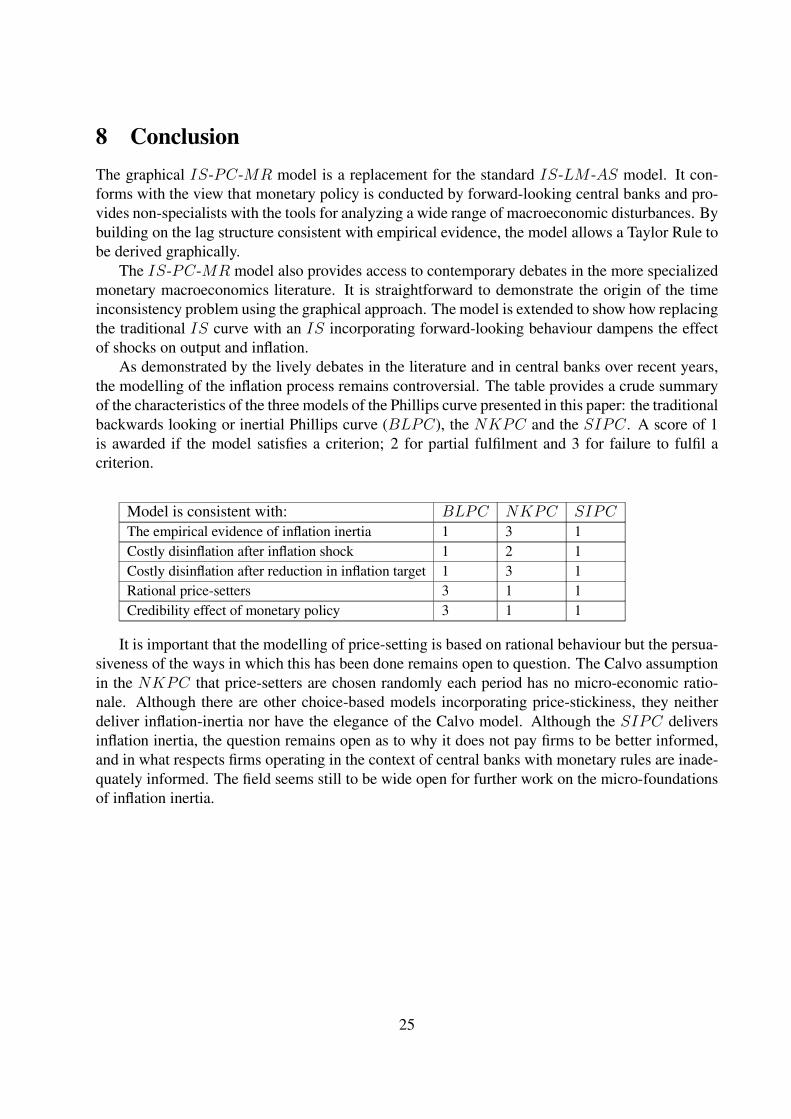
the modelling of the inflation process remains controversial. The table provides a crude summary

of the characteristics of the three models of the Phillips curve presented in this paper: the traditional

backwards looking or inertial Phillips curve (BLPC), the NKPC and the SIPC. A score of 1

is awarded if the model satisfies a criterion; 2 for partial fulfilment and 3 for failure to fulfil a

criterion.

Model is consistent with: BLPC NKPC SIPCThe empirical evidence of inflation inertia 1 3 1

Costly disinflation after inflation shock 1 2 1

Costly disinflation after reduction in inflation target 1 3 1

Rational price-setters 3 1 1

Credibility effect of monetary policy 3 1 1

It is important that the modelling of price-setting is based on rational behaviour but the persua-

siveness of the ways in which this has been done remains open to question. The Calvo assumption

in the NKPC that price-setters are chosen randomly each period has no micro-economic ratio-

nale. Although there are other choice-based models incorporating price-stickiness, they neither

deliver inflation-inertia nor have the elegance of the Calvo model. Although the SIPC delivers

inflation inertia, the question remains open as to why it does not pay firms to be better informed,

and in what respects firms operating in the context of central banks with monetary rules are inade-

quately informed. The field seems still to be wide open for further work on the micro-foundations

of inflation inertia.

25

Appendix

Appendix 1. Deriving the Monetary Policy Rule in the IS-PC-MR model

The central bank aims to minimize:

L =1

2

[(y − ye)

2 + β(π − πT

)2]

subject to the Phillips curve: π = π−1+α(y−ye). Solving this minimization problem delivers the

monetary rule: y− ye = −αβ(π− πT ), which implies that the slope of the monetary rule curve as

shown in Fig.7 is γ = 1αβ

, reflecting both the slope of the Phillips curve and the inflation aversion

of the central bank. In its Taylor Rule form, the monetary rule is:

r0 − rS =1

(α + γ)a

[(π0 − πT

)+ α(y0 − ye)

].

Inflation aversion shows up in the coefficient 1(α+γ)a

: it therefore affects both elements of the Taylor

Rule equally.

We can see that Taylor’s weights of 0.5 and 0.5 arise when the IS curve, the Phillips curves

and the MR curve all have a slope of one (or more precisely in the case of the IS and the MRof minus one). To consider the implications for the central bank’s reaction to current inflation and

output information when the key parameters differ from one, we take each in turn, keeping the

other two equal to one. We begin with the monetary rule curve, the slope of which depends on

both the slope of the Phillips curve and on the degree of inflation-aversion of the central bank since

γ = 1αβ

. Since β is the weight on inflation in the central bank’s loss function and holding α = 1, a

value of β > 1 reflects more inflation aversion on the part of the central bank than in our base-line

case. Hence the MR-curve is flatter. The implications for the central bank are unambiguous and

intuitive: the central bank will raise the interest rate by more in the face of a given inflation or

output shock.

Turning to the Phillips curve, as we have seen, its slope α affects the relative weight on inflation

and output in the Taylor Rule. For α > 1, the Phillips curves are steeper and the MR curve is flatter.

There are two implications, which go in opposite directions. First, a more restrictive interest rate

reaction is optimal to deal with any given increase in output because this will have a bigger effect

on inflation than with α = 1 (this is the result of the flatter MR-curve). But on the other hand,

a given rise in the interest rate will have a bigger negative effect on inflation. These two effects

imply that with α > 1, the balance between the coefficients changes: the coefficient on (π0− πT )

goes down — so the central bank reacts less to an inflation shock whereas the coefficient on (y0−ye) goes up — the central bank reacts more to an output shock as compared with the equal weights

in the Taylor rule.

Finally, if a > 1 this means that the effect on demand of a change in the interest rate increases:

the IS-curve is flatter. This has a predictable effect on the central bank policy rule: a rise in a above

one, reduces the coefficients on both the inflation and output deviations. Since a given interest rate

response has a bigger effect, the central bank should react less to any given shock.

26

x10 x0 x0

*x1*

IS0IS-1

rS0

rS1

r*

IS1 IS*

MR

r0

π2= π1*+ αx1

*

πT

π1*

aggregate demand shock

π1

π2= π1+ αx1

π1= πT+ αx0

π2

A

A'

Z'

Z

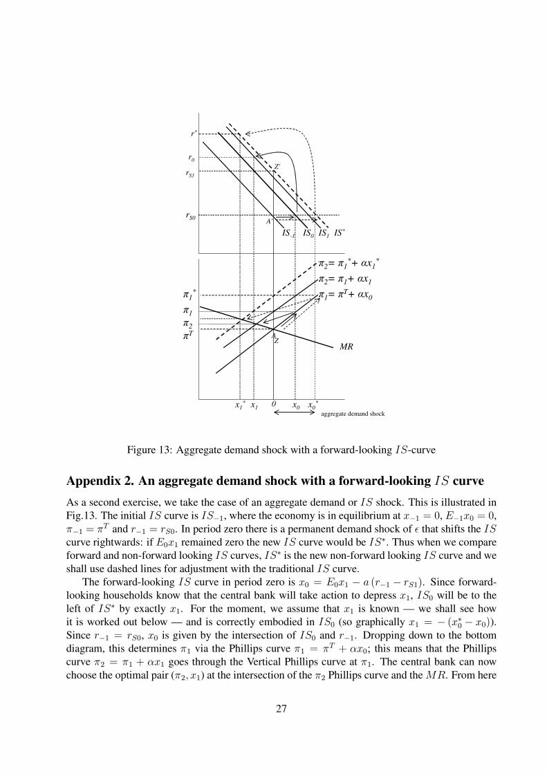
Figure 13: Aggregate demand shock with a forward-looking IS-curve

Appendix 2. An aggregate demand shock with a forward-looking IS curve

As a second exercise, we take the case of an aggregate demand or IS shock. This is illustrated in

Fig.13. The initial IS curve is IS−1, where the economy is in equilibrium at x−1 = 0, E−1x0 = 0,π−1 = πT and r−1 = rS0. In period zero there is a permanent demand shock of ǫ that shifts the IScurve rightwards: if E0x1 remained zero the new IS curve would be IS∗. Thus when we compare

forward and non-forward looking IS curves, IS∗ is the new non-forward looking IS curve and we

shall use dashed lines for adjustment with the traditional IS curve.

The forward-looking IS curve in period zero is x0 = E0x1 − a (r−1 − rS1). Since forward-

looking households know that the central bank will take action to depress x1, IS0 will be to the

left of IS∗ by exactly x1. For the moment, we assume that x1 is known — we shall see how

it is worked out below — and is correctly embodied in IS0 (so graphically x1 = − (x∗0 − x0)).Since r−1 = rS0, x0 is given by the intersection of IS0 and r−1. Dropping down to the bottom

diagram, this determines π1 via the Phillips curve π1 = πT + αx0; this means that the Phillips

curve π2 = π1 + αx1 goes through the Vertical Phillips curve at π1. The central bank can now

choose the optimal pair (π2, x1) at the intersection of the π2 Phillips curve and the MR. From here

27

it is easy to work out the central bank’s choices of the pairs (π3, x2), (π4, x3) and so on from the

intersections of the MR with the relevant Phillips curves. The path of adjustment is shown by the

arrows in the lower panel.

How does the central bank use its choice of the interest rate to produce this adjustment path?

We have already worked out the values of x1, x2, x3, . . .which the central bank engineers during

the adjustment process. The IS diagram can now be used to find the values of r0, r1, r2, . . . which

the central bank needs to set for this pattern of excess supply. Starting with r0, the relevant IScurve is IS0:

x1 = x2 − a (r0 − rS,1)

and r0 is now the interest rate at the intersection of IS0 and the vertical x1 line. Similarly, since

x2 = x3 − a (r1 − rS,1)

and r1 is the interest rate at the intersection of IS1 and the vertical x2 line. Thus the interest rate

is raised from its original level of r−1 = rS,0 to r0 and then is gradually adjusted back down to the

new equilibrium at rS,1. This is shown by the arrow in the IS diagram.

Fig.13 shows clearly that the forward-looking IS curve reduces the amplitude of both output

and interest rate changes. Absent its forward-looking component, the shocked IS curve is the

dashed line, IS∗, x0 = −a (r−1 − rS,1) so that with r−1 = rS,0 initial excess demand is x∗0. This

generates the dashed π2 Phillips curve (π2 = π∗1 + αx∗1), and hence x∗1, and in turn r∗ > r0. The

return to equilibrium is down the dashed IS∗ line.

Appendix 3. The New Keynesian Phillips Curve

Deriving the New Keynesian Phillips Curve

The standard derivation of the NKPC is somewhat lengthy. By cutting a few corners, however,

there is a much simpler derivation, which makes the intuition behind the equation clearer. Let p∗

be the log of the price set by the δ percent of price setters at time t. Hence, since the other 1 − δfirms will retain last period’s price level, the current price level is given by

pt = δp∗t + (1− δ) pt−1

Since πt ≡ pt − pt−1 and the inflation rate of those who set their prices at t is π∗t ≡ p∗t − pt−1, it is

easy to see that πt = δπ∗t .What inflation rate π∗ will price setters want in the current period if they have the chance to

reset their prices? Given imperfect competition, they will want to raise the relative price of their

differentiated products if there is excess demand, i.e. x > 0 and vice versa if x < 0. Hence, for

x > 0, they will want an inflation rate above the aggregate: π∗ = π + αx. However, the price they

set now, p∗, has to last until they next get a chance to reset their prices. There is a (1 − δ) chance

that they will not be able to reset in t+ 1, a (1− δ)2 chance in t+ 2, etc. In addition they care less

about future periods because of the discount factor θ. Thus they attach a value of 1 to having the

right inflation rate in the current period, θ(1− δ) in t+ 1, θ2(1− δ)2 in t+ 2, and so on. So their

chosen π∗ has to be the correct rate for the current period plus the correct rate for t + 1 weighted

by θ(1− δ), and so on. Hence:

π∗t =[(πt + αxt) + θ (1− δ)Etπt+1 + αEtxt+1) + θ2 (1− δ)2Etπt+2 + αEtxt+2) + ...

].

28

Since πt = δπ∗t , we have

πt = δ [(πt + αxt) + θ (1− δ)Etπt+1 + αEtxt+1) + ...] .

This enables us to make a simple transformation: leading both sides by one period and multiplying

both sides by θ(1− δ) generates

θ (1− δ)Etπt+1 = θ (1− δ) δ [(Etπt+1 + αEtxt+1) + θ (1− δ) (Etπt+2 + αEtxt+2) + ...]

and subtracting this from the previous equation implies

πt = δπt + αδxt + θ (1− δ)Etπt+1.

When rearranged, this produces the New Keynesian Phillips Curve:

πt =αδ

1− δxt + θEtπt+1.

We turn now to the question of what is the rationally expected value of πt+1. To find this, we

need first to derive the monetary rule. Just as before, the central bank minimises a loss function

and to simplify the notation, it is assumed that the central bank’s inflation target is zero. The loss

function can be written explicitly as

L =1

2

(x2t + βπ2t

)

and is minimized subject to the constraint imposed by the NKPC. Since the central bank takes

expectations of future inflation by private agents as given, and assuming it can re-maximise each

period, this implies that there is an MR curve as follows:

πt = −γxt,

where γ = 1−δδαβ

. For ease of exposition, we follow NKPC theorists and assume there are no time

lags from the interest rate to output or from output to inflation.

The next step is to use rational expectations to evaluate the expected future inflation rate,

Etπt+1. It is not difficult to show that expected future inflation is equal to the target, i.e. Etπt+1 =0. First, the NKPC and the MR must both hold in each period: πt = −γxt and πt =

1βγxt +

θEtπt+1. Eliminating xt from the pair of equations, this implies

πt =

(θ

1 + 1βγ2

)

Etπt+1

where we define the term in brackets as τ ; it lies between zero and one. Since the MR and

NKPC hold each period, Etπt+i = τEtπt+i+1 for all i. Hence if we rule out the possibility that

Etπt+i →∞ with i, we have the result Etπt+i = 0 (or in the case where the inflation target is not

zero, Etπt+i = πT ).

29

Deriving Etπt+1 in the NKPC with autocorrelated cost-push added

Clarida et al. (1999) attempt to build more realistic results into their model by introducing into

the NKPC an exogenous “cost-push” factor, c, in effect an inflation shock, the effect of which is

assumed to diminish over time. Because this development is both important and difficult to follow

in their article it is explained here. As far as we can see, it lacks microfoundations.

The NKPC now becomes

πt =αδ

1− δxt + θEtπt+1 + ct

where ct = ρct−1+εt, with ρ a positive constant less than one and εt, a random variable with mean

zero that is not autocorrelated. The assumed form of the cost-push factor, ct, is crucial in generating

inflation dynamics in the NKPC model: the cost-push this period is a fraction of cost-push last

period (plus a random component).

The introduction of the cost-push factor makes evaluating Etπt+1 slightly more difficult. Here

is how it is done. With rational expectations and dropping the expectation operator to simplify the

notation, we have the Phillips curve:

πt+1 = α

(δ

1− δ

)xt+1 + θπt+2 + ρct

and the monetary rule:

πt+1 = −γxt+1,

which together imply

πt+1 = θbπt+2 + ρbct

where b ≡ 1/(1 + (βγ2)

−1); and working out πt+2 the same way:

πt+2 = θbπt+3 + ρ2bct.

Note that the impact of ct declines by ρ each period. Successively substituting, we get

πt+1 = bρct[1 + θbρ+ θ2b2ρ2...

]=

b

1− θbρρct.

For simplicity and restoring the expectation operator, we write this as:

Etπt+1 = λρct,

where 0 < λ < 1. This means that the ‘new’ NKPC is given by

πt =αδ

1− δxt + θEtπt+1 + ct =

αδ

1− δxt + (1 + θλρ)ct.

The NKPC is shown in Fig.14 and the term (1+ θλρ)ct is measured by the rate of inflation when

output is at equilibrium.

The geometry of the model looks similar to that of the standard IS-PC-MR model. The key

difference centres on what determines the position of the Phillips curve and on what shifts it. In

30

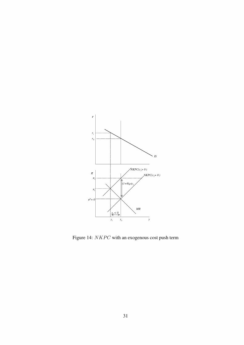
r

rS

NKPC(ct= 0 )

MR

IS

y

π

πT= 0

yt ye

rt

NKPC(ct> 0 )

πt

π1

xt < 0

(1+θλρ)ct

Figure 14: NKPC with an exogenous cost push term

31

the IS-PC-MR model the Phillips curve is shifted by inertial inflation, with the consequence that

the Phillips curve shifts endogenously as inflation adjusts. With the NKPC, the exogenous cost

push term, ct, fixes the position of the Phillips curve and the assumption that this becomes weaker

at the rate ρ leads the NKPC to shift. To see how this works, we need to assume that the cost

push effect persists, i.e. ρ > 0 since if ρ = 0, the expected future inflation term disappears. It is

simplest to assume that ct = c∗ and that εt+i = 0 for all i > 0. In this case the NKPC at t is

πt =αδ1−δ

xt + (1 + θλρ)c∗, where Etπt+1 = λρc∗. So again determining πt by the intersection of

MR and NKPC we get

πt =1 + θλρ

[1 + (1/βγ2)]c∗

Bearing in mind that the influence of c∗ diminishes exponentially by ρ each period, the NKPC in

period t+ 1 is πt+1 =αδ1−δ

xt+1 + (1 + θλρ)ρc∗ and hence

πt+1 =1 + θλρ

[1 + (1/βγ2)]ρc∗ = ρπt.

So with ρ > 0 there is a gradual move of the NKPC down the MR curve and the economy moves

back to equilibrium along the path from B to C and back to A as shown in Fig.15 with the central

bank adjusting the interest rate appropriately as shown in the upper panel. But note that any one

period inflation shock has no effect on next period’s inflation: in so far as inflation persists in this

ad hoc model it is driven purely by the autocorrelation of past shocks.

32

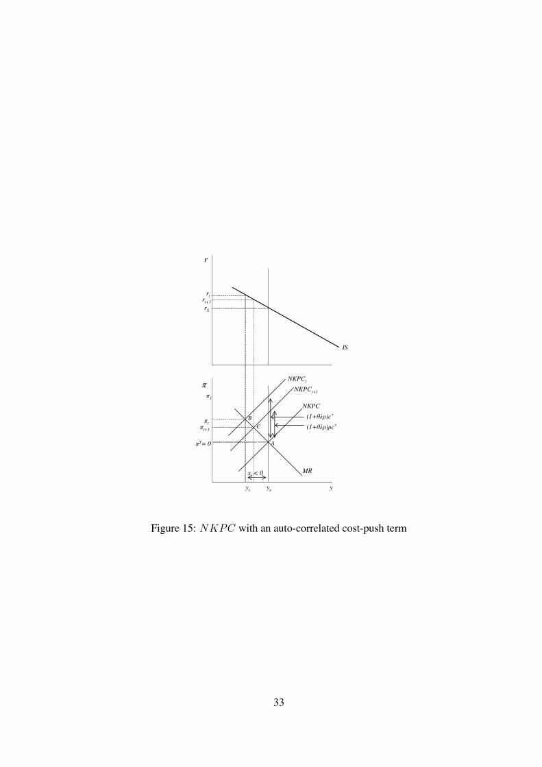
r

rS

NKPC

MR

IS

y

π

πT= 0

yt ye

rt

NKPCt

πt

π1

xt < 0

(1+θλρ)c*

(1+θλρ)ρc*

NKPCt+1

πt+1

A

B

C

rt+1

Figure 15: NKPC with an auto-correlated cost-push term

33

References

Allsopp, Christopher and David Vines (2000). “The assessment: macroeconomic policy”

Oxford Review of Economic Policy Vol. 16, No. 4, 1-32.

Ball, Laurence (1994). “Credible Disinflation with Staggered Price-Setting” American Eco-

nomic Review, Vol. 84, No. 1, 282-289.

Bank of England (1999) “The Transmission of Monetary Policy”

http://www.bankofengland.co.uk/montrans.pdf

Bean, Charles (1998). “The New UK Monetary Arrangements: A View from the Literature”,

Economic Journal 108, 1795-1808.

Calvo, Guillermo A. (1983) “Staggered Prices in a Utility Maximizing Framework”, Journal

of Monetary Economics, 12, 3, 383-98.

Clarida, Richard, Jordi Gali and Mark Gertler (1999). “The Science of Monetary Policy: A

New Keynesian Perspective”, Journal of Economic Literature. 37:4, 1661-1707.

Estrella, Arturo and Jeffrey C. Fuhrer (2002). “Dynamic Inconsistencies: Counterfactual Im-

plications of a Class of Rational-Expectations Models” American Economic Review Vol. 92 No.

4, 1013-1028.

Fuhrer, Jeff and George Moore (1995). “Inflation Persistence” The Quarterly Journal of Eco-

nomics, Vol. 110, No. 1. (Feb., 1995), 127-159.

Goodfriend, Marvin and Robert King (1997) “The New Neoclassical Synthesis and the Role

of Monetary Policy,” NBER Macroeconomics Annual, 231-283.

Gordon, Robert (1997) “The Time-Varying NAIRU and Its Implications for Monetary Policy,”

Journal of Economic Perspectives, Winter, 11-32.

McCallum, Bennett T. and Edward Nelson (1999). “An optimizing IS-LM specification for

monetary policy and business cycle analysis”, Journal of Money, Credit and Banking, Vol. 31, No.

3, Part 1. 296-316.

Mankiw, N. Gregory and Ricardo Reis (2002). “Sticky Information versus Sticky Prices: A

Proposal to Replace the New Keynesian Phillips Curve”, The Quarterly Journal of Economics,

117(4), 1295-1328.

Nelson, Edward (1998). “Sluggish Inflation and Optimizing Models of the Business Cycle”,

Journal of Monetary Economics, 42, 303-322.

Romer, David (2000). “Keynesian Macroeconomics with the LM Curve” Journal of Economic

Perspectives, 14:2, Spring, 149-169.

Staiger, Douglas, James Stock and Mark Watson (1997) “The NAIRU, Unemployment, and

Monetary Policy,” Journal of Economic Perspectives, vol. 11 Winter 1997, 33- 51.

Taylor, John B. (1993). “Discretion versus policy rules in practice” Carnegie-Rochester Con-

ference Series on Public Policy, 39(1), 195-214.

Taylor, John B. (2000). “Teaching Modern Macroeconomics at the Principles Level”, Ameri-

can Economic Review. Papers and Proceedings. 90 (2), 90-94.

Walsh, Carl E. (2002) “Teaching Inflation Targeting: An Analysis for Intermediate Macro”.

Journal of Economic Education 33 (4), Fall 2002, 333-347.

Walsh, Carl E. (2003) Monetary Theory and Policy 2nd edition MIT Press: Cambridge Mass.

34

Woodford, Michael (2003). Interest and Prices: Foundations of a Theory of Monetary Policy.

Princeton University Press: Princeton.

35