Embed Size (px)
Citation preview
THE 3-EQUATION MODELStefania Paredes Fuentes
Department of Economics, S2.121 University of Warwick
Money & Banking WESS 2016
THE 3-EQUATION MODEL AND MACROECONOMIC POLICY
• Demand shocks, supply shocks
• Government intervention - stabilisation policy
• Inflation targeting - monetary policy regime
Stefania Paredes Fuentes Money and BankingWESS 2016
THE 3-EQUATION MODEL AND MACROECONOMIC POLICY
Stefania Paredes Fuentes Money and BankingWESS 2016
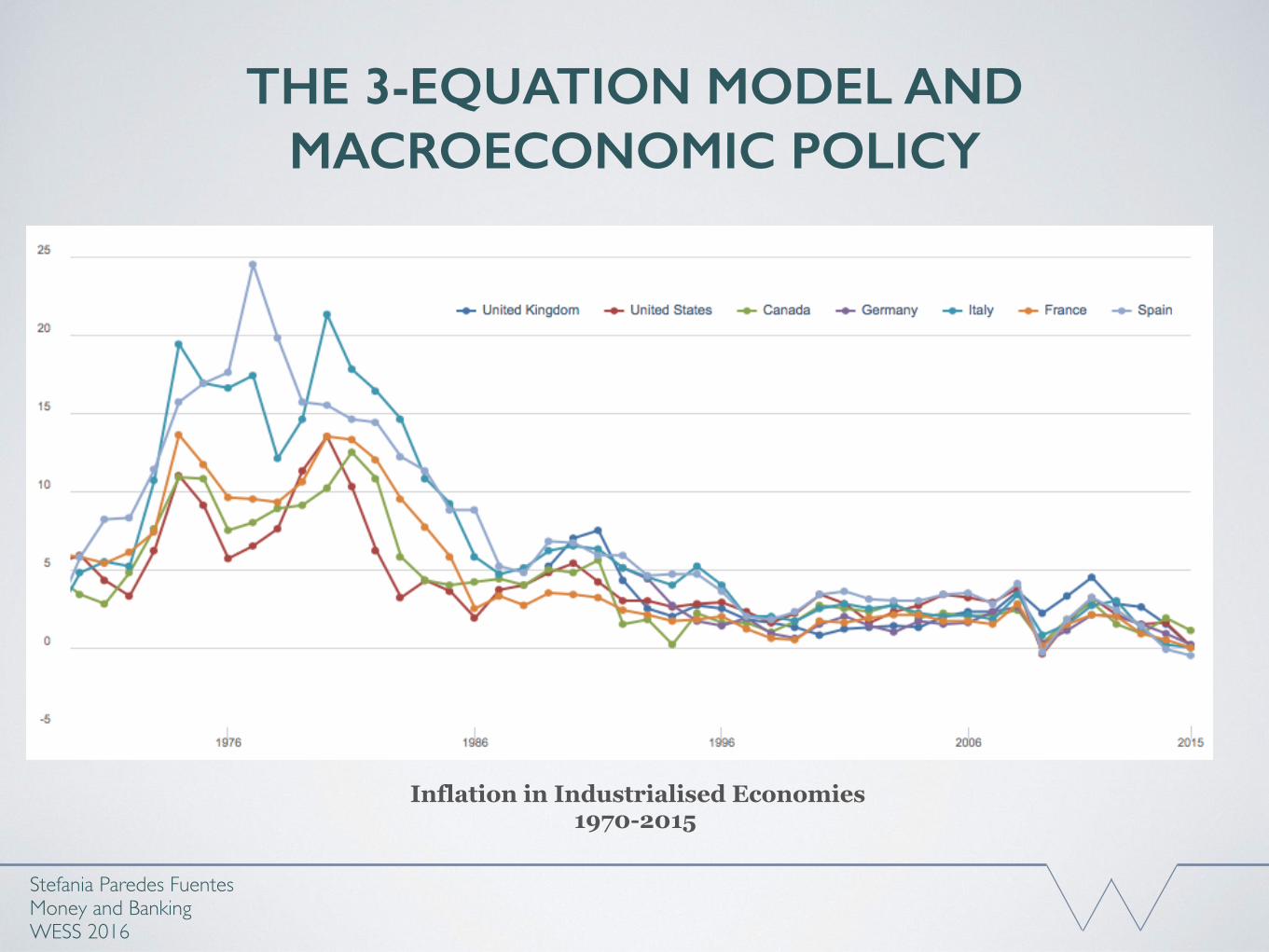
Inflation in Industrialised Economies 1970-2015
THE 3-EQUATION MODEL AND MACROECONOMIC POLICY
Stefania Paredes Fuentes Money and BankingWESS 2016
THE 3-EQUATION MODEL AND MACROECONOMIC POLICY
• (1945 - 1971: Bretton Woods fixed exchange rate regime)
• 1970s - 1980s From the Quantity Theory of Money: controlling the growth rate of the money supply allow policy makers to control the rate of inflation - 1974 - monetary targeting in Germany and Switzerland
• For a monetary targeting to be successful:(1) the CB met be able to control the chosen monetary aggregate,(2) the relationship between inflation and the targeted monetary aggregate must be reliable
Stefania Paredes Fuentes Money and BankingWESS 2016
Monetary Policy
THE 3-EQUATION MODEL AND MACROECONOMIC POLICY
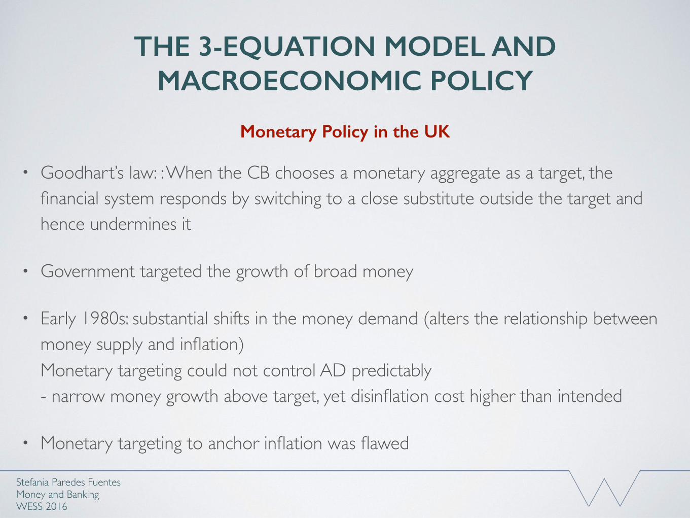
• Goodhart’s law: : When the CB chooses a monetary aggregate as a target, the financial system responds by switching to a close substitute outside the target and hence undermines it
• Government targeted the growth of broad money
• Early 1980s: substantial shifts in the money demand (alters the relationship between money supply and inflation) Monetary targeting could not control AD predictably- narrow money growth above target, yet disinflation cost higher than intended
• Monetary targeting to anchor inflation was flawed
Stefania Paredes Fuentes Money and BankingWESS 2016
Monetary Policy in the UK

THE 3-EQUATION MODEL AND MACROECONOMIC POLICY
Stefania Paredes Fuentes Money and BankingWESS 2016
Monetary Policy in the UK
inflation = 18% unemployment = 6.9%
inflation = 4-5% unemployment = 11-12%
THE 3-EQUATION MODEL AND MACROECONOMIC POLICY
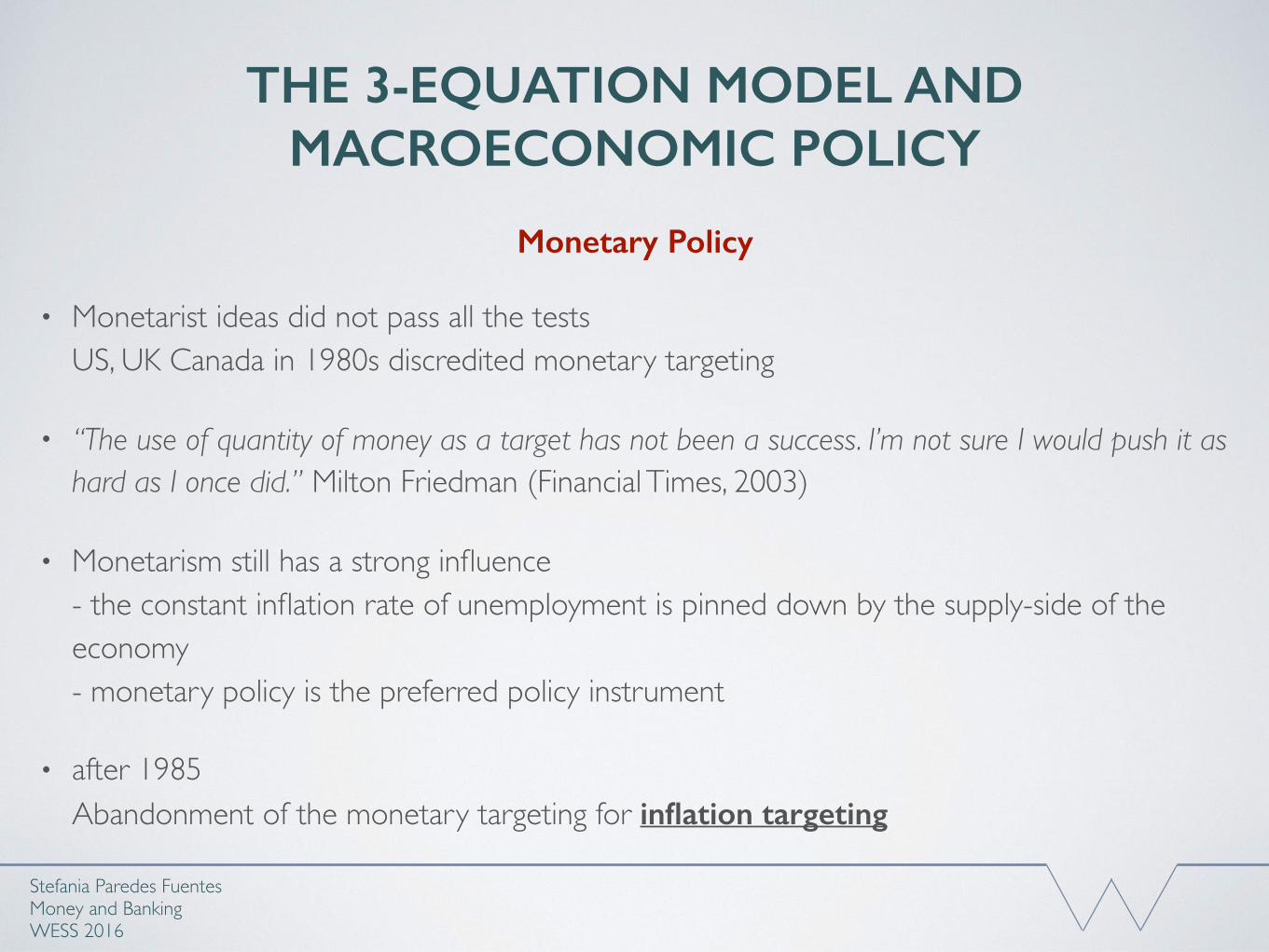
• Monetarist ideas did not pass all the testsUS, UK Canada in 1980s discredited monetary targeting
• “The use of quantity of money as a target has not been a success. I’m not sure I would push it as hard as I once did.” Milton Friedman (Financial Times, 2003)
• Monetarism still has a strong influence - the constant inflation rate of unemployment is pinned down by the supply-side of the economy- monetary policy is the preferred policy instrument
• after 1985Abandonment of the monetary targeting for inflation targeting
Stefania Paredes Fuentes Money and BankingWESS 2016
Monetary Policy
THE 3-EQUATION MODEL AND MACROECONOMIC POLICY
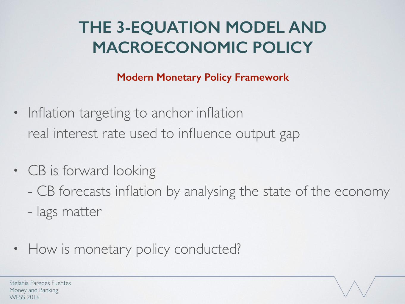
• Inflation targeting to anchor inflation real interest rate used to influence output gap
• CB is forward looking- CB forecasts inflation by analysing the state of the economy - lags matter
• How is monetary policy conducted?
Stefania Paredes Fuentes Money and BankingWESS 2016
Modern Monetary Policy Framework
THE 3-EQUATION MODEL AND MACROECONOMIC POLICY
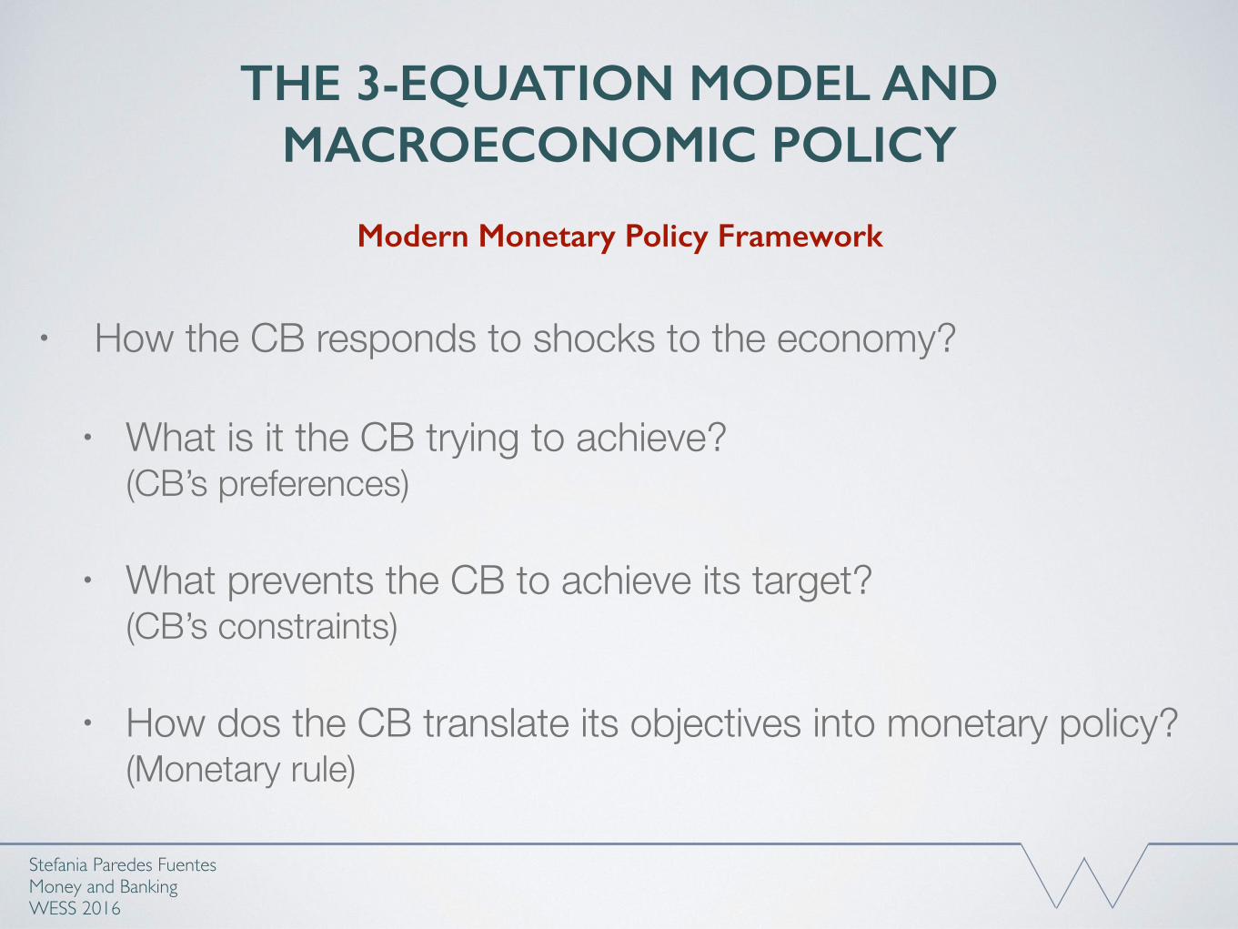
• How the CB responds to shocks to the economy?
• What is it the CB trying to achieve?(CB’s preferences)
• What prevents the CB to achieve its target?(CB’s constraints)
• How dos the CB translate its objectives into monetary policy?(Monetary rule)
Stefania Paredes Fuentes Money and BankingWESS 2016
Modern Monetary Policy Framework
THE 3-EQUATION MODEL AND MACROECONOMIC POLICY
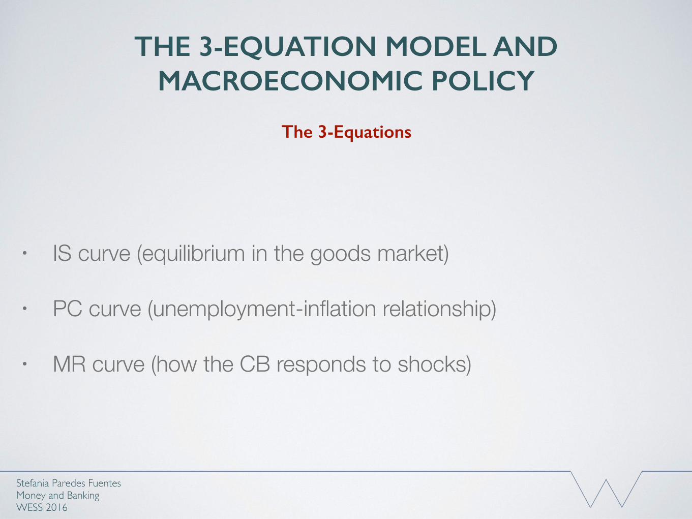
• IS curve (equilibrium in the goods market)
• PC curve (unemployment-inflation relationship)
• MR curve (how the CB responds to shocks)
Stefania Paredes Fuentes Money and BankingWESS 2016
The 3-Equations
THE 3-EQUATION MODEL AND MACROECONOMIC POLICY
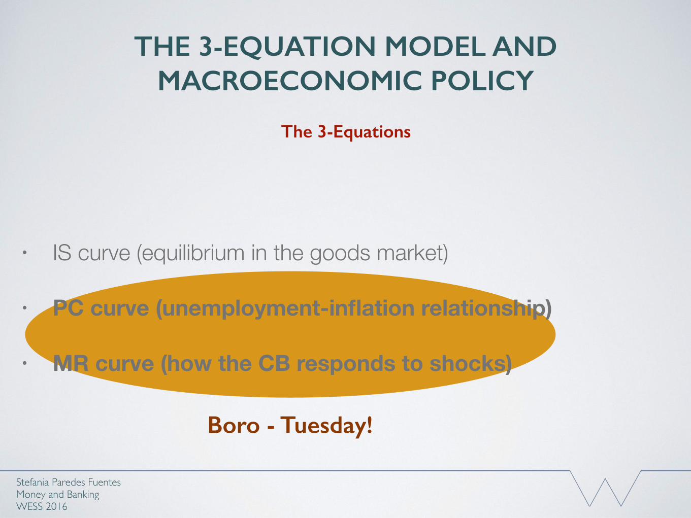
• IS curve (equilibrium in the goods market)
• PC curve (unemployment-inflation relationship)
• MR curve (how the CB responds to shocks)
Stefania Paredes Fuentes Money and BankingWESS 2016
The 3-Equations
Boro - Tuesday!
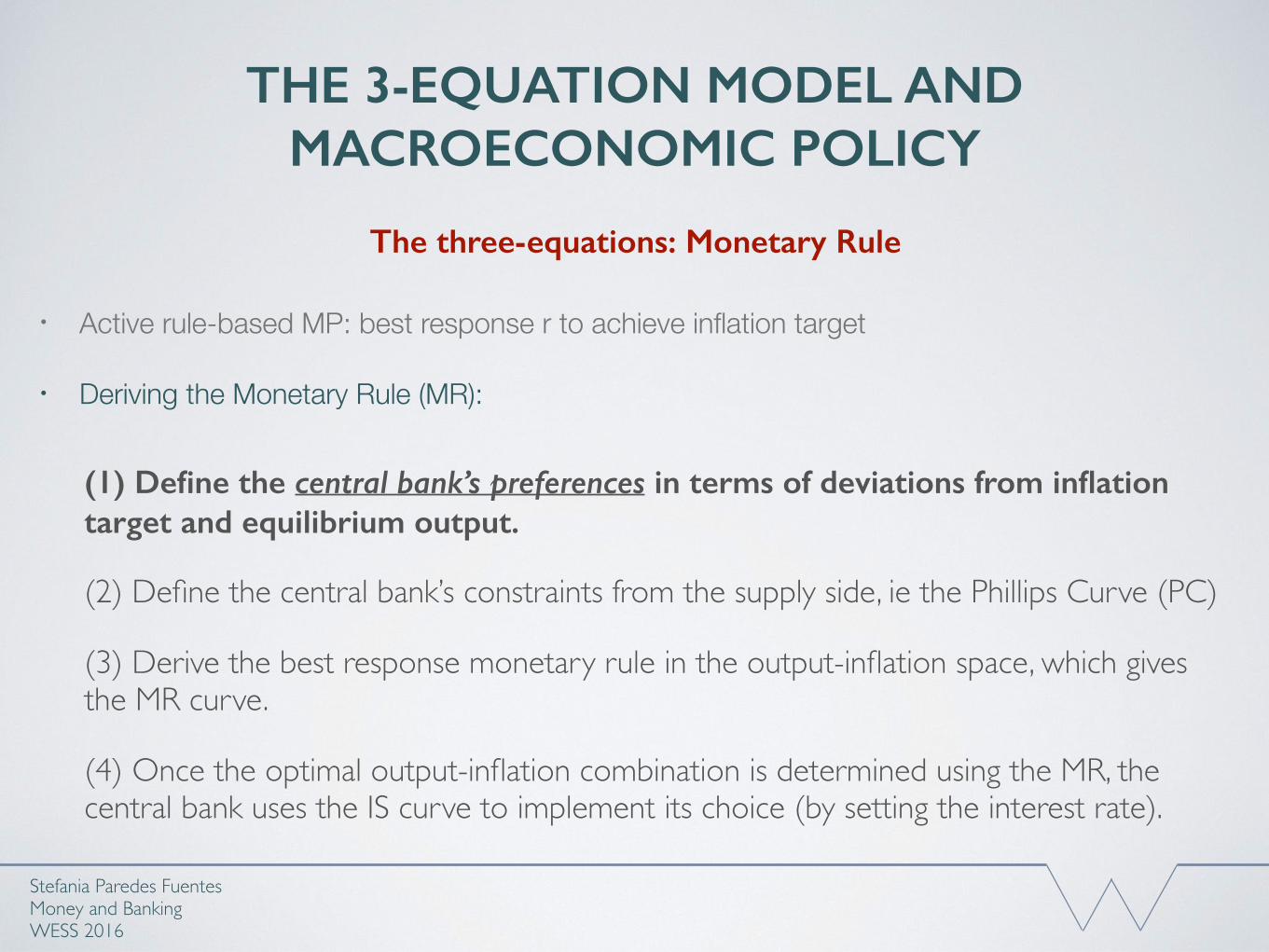
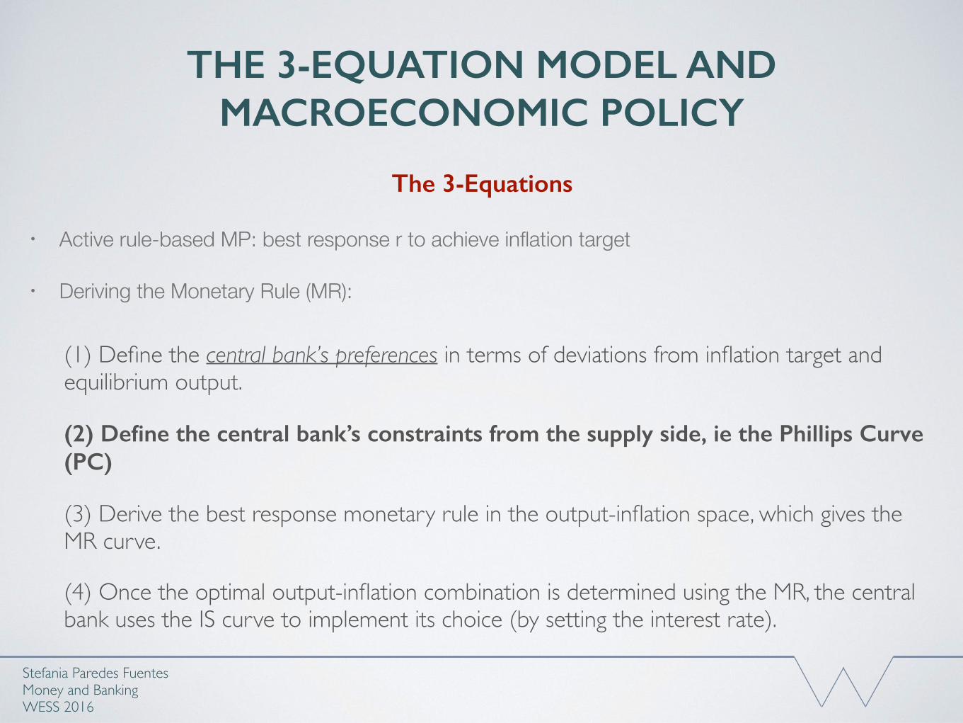
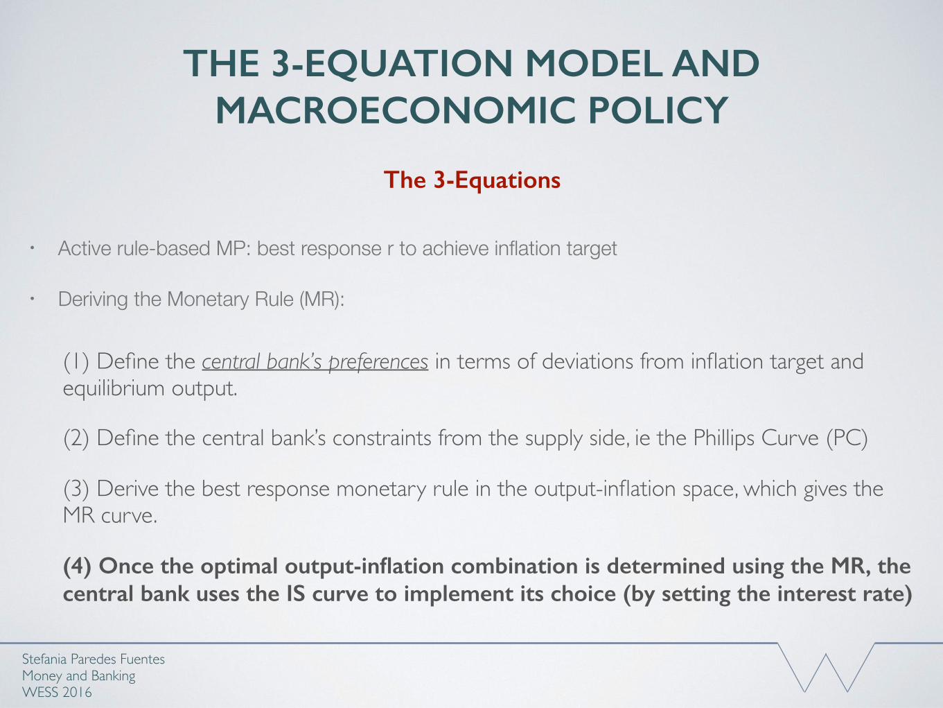
• Active rule-based MP: best response r to achieve inflation target
• Deriving the Monetary Rule (MR):
(1) Define the central bank’s preferences in terms of deviations from inflation target and equilibrium output.
(2) Define the central bank’s constraints from the supply side, ie the Phillips Curve (PC)
(3) Derive the best response monetary rule in the output-inflation space, which gives the MR curve.
(4) Once the optimal output-inflation combination is determined using the MR, the central bank uses the IS curve to implement its choice (by setting the interest rate).
THE 3-EQUATION MODEL AND MACROECONOMIC POLICY
Stefania Paredes Fuentes Money and BankingWESS 2016
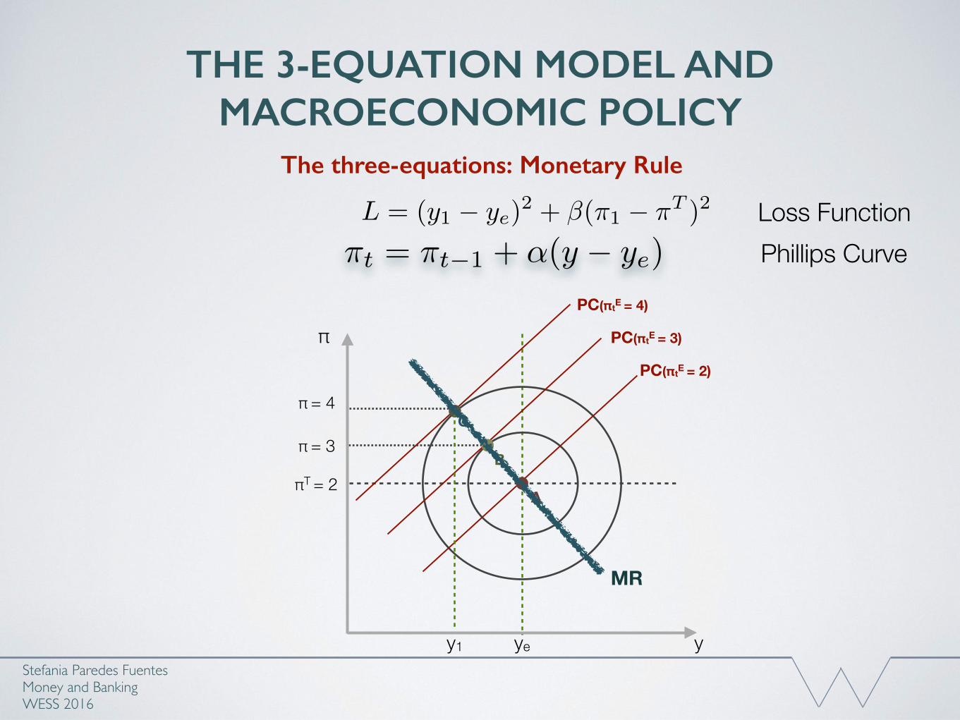
The three-equations: Monetary Rule
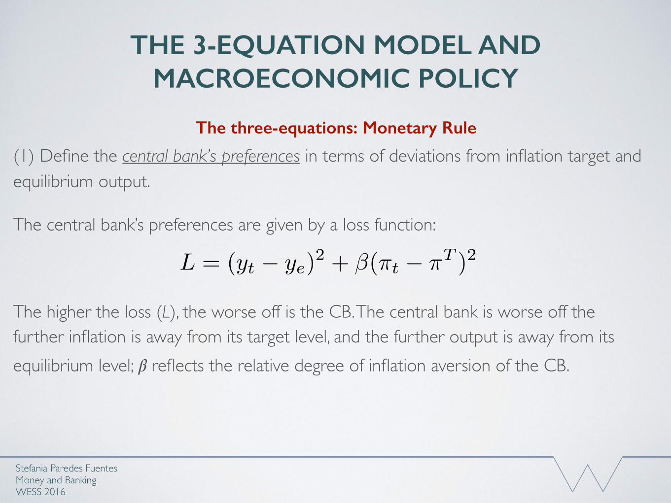
(1) Define the central bank’s preferences in terms of deviations from inflation target and equilibrium output.
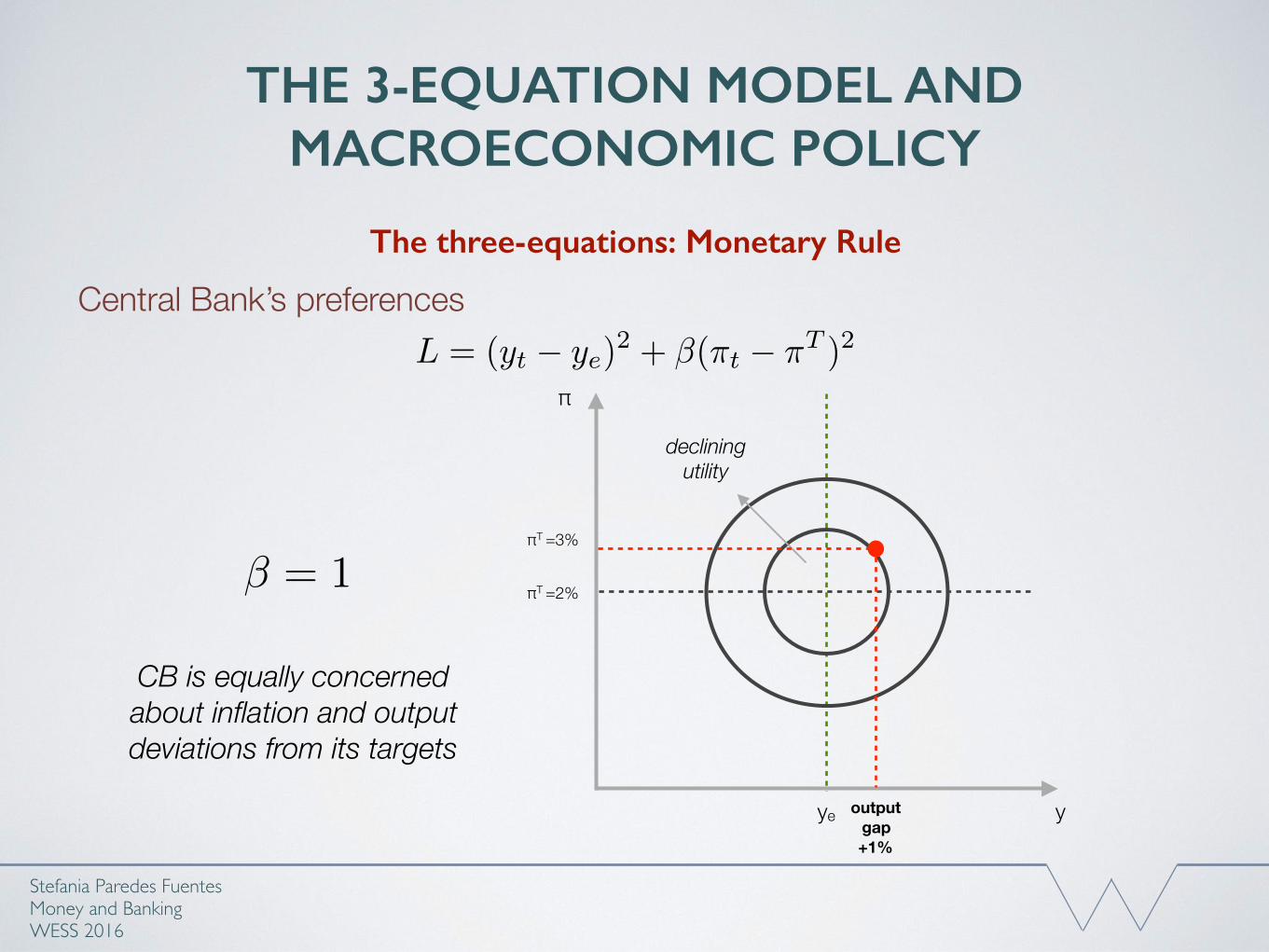
The central bank’s preferences are given by a loss function:
The higher the loss (L), the worse off is the CB. The central bank is worse off the further inflation is away from its target level, and the further output is away from its equilibrium level; 𝛽 reflects the relative degree of inflation aversion of the CB.
THE 3-EQUATION MODEL AND MACROECONOMIC POLICY
Stefania Paredes Fuentes Money and BankingWESS 2016
L = (yt � ye)2 + �(⇡t � ⇡T )2
The three-equations: Monetary Rule

THE 3-EQUATION MODEL AND MACROECONOMIC POLICY
Stefania Paredes Fuentes Money and BankingWESS 2016
Central Bank’s preferencesL = (yt � ye)
2 + �(⇡t � ⇡T )2
y
π
ye
πT
declining utility
Bliss point
The three-equations: Monetary Rule
THE 3-EQUATION MODEL AND MACROECONOMIC POLICY
Stefania Paredes Fuentes Money and BankingWESS 2016
Central Bank’s preferencesL = (yt � ye)
2 + �(⇡t � ⇡T )2
CB is equally concerned about inflation and output deviations from its targets
� = 1
y
π
ye
declining utility
πT =2%
πT =3%
output gap+1%
The three-equations: Monetary Rule
THE 3-EQUATION MODEL AND MACROECONOMIC POLICY
Stefania Paredes Fuentes Money and BankingWESS 2016
Central Bank’s preferencesL = (yt � ye)
2 + �(⇡t � ⇡T )2
y
π
ye
πT =2%
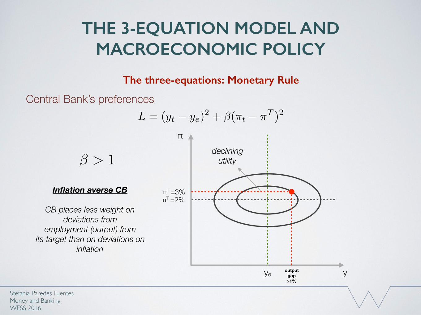
declining utility� > 1
Inflation averse CB
CB places less weight on deviations from
employment (output) from its target than on deviations on
inflation
πT =3%
output gap>1%
The three-equations: Monetary Rule
THE 3-EQUATION MODEL AND MACROECONOMIC POLICY
Stefania Paredes Fuentes Money and BankingWESS 2016
Central Bank’s preferencesL = (yt � ye)
2 + �(⇡t � ⇡T )2
y
π
ye
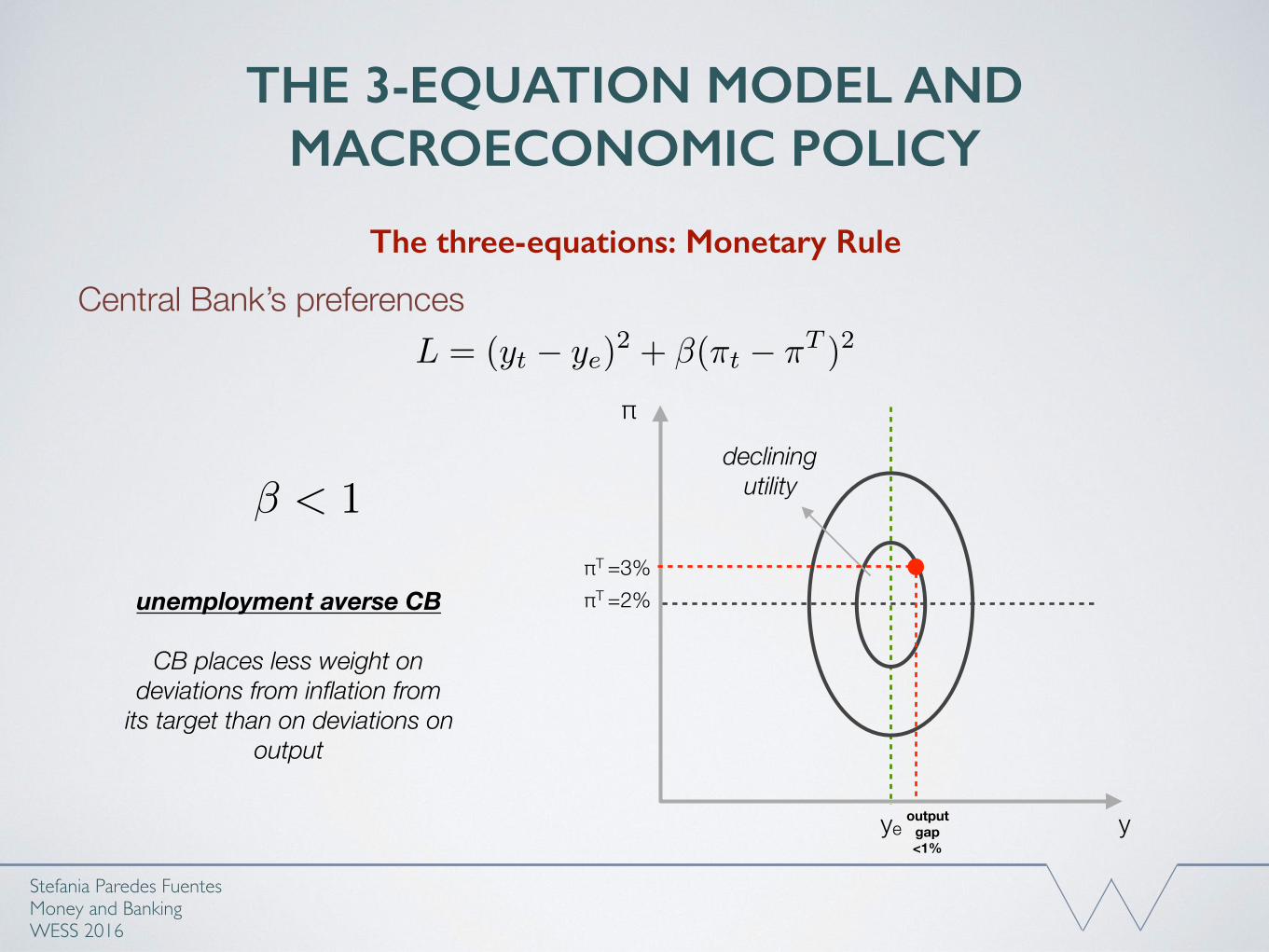
declining utility� < 1
unemployment averse CB
CB places less weight on deviations from inflation from
its target than on deviations on output
πT =2%πT =3%
output gap<1%
The three-equations: Monetary Rule
• Active rule-based MP: best response r to achieve inflation target
• Deriving the Monetary Rule (MR):
(1) Define the central bank’s preferences in terms of deviations from inflation target and equilibrium output.
(2) Define the central bank’s constraints from the supply side, ie the Phillips Curve (PC)
(3) Derive the best response monetary rule in the output-inflation space, which gives the MR curve.
(4) Once the optimal output-inflation combination is determined using the MR, the central bank uses the IS curve to implement its choice (by setting the interest rate).
THE 3-EQUATION MODEL AND MACROECONOMIC POLICY
Stefania Paredes Fuentes Money and BankingWESS 2016
The 3-Equations
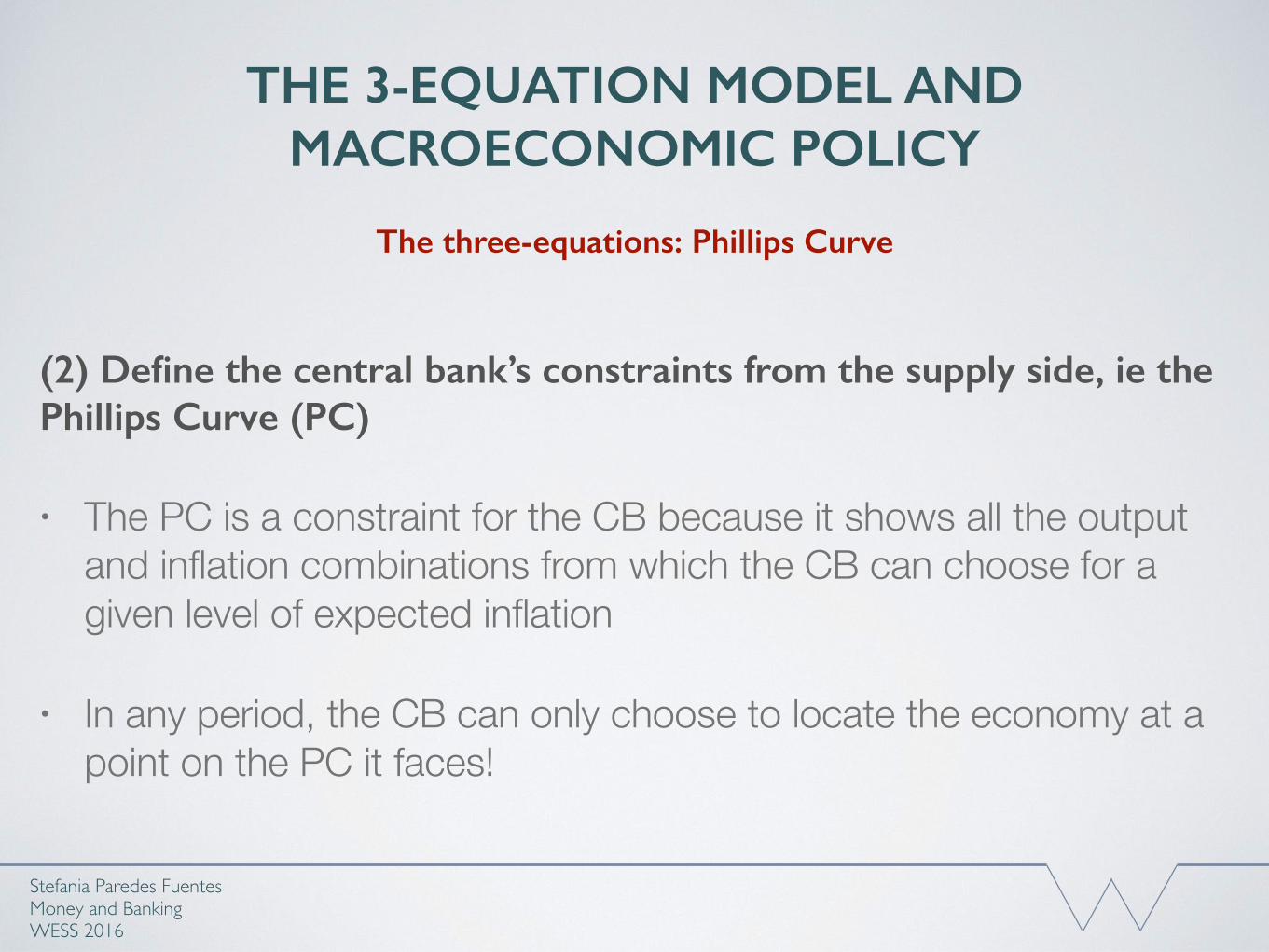
(2) Define the central bank’s constraints from the supply side, ie the Phillips Curve (PC)
• The PC is a constraint for the CB because it shows all the output and inflation combinations from which the CB can choose for a given level of expected inflation
• In any period, the CB can only choose to locate the economy at a point on the PC it faces!
THE 3-EQUATION MODEL AND MACROECONOMIC POLICY
Stefania Paredes Fuentes Money and BankingWESS 2016
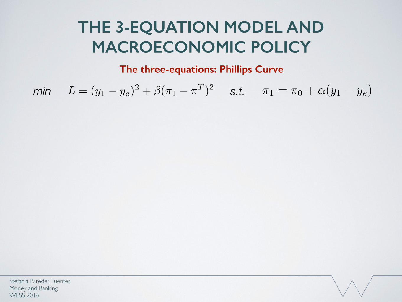
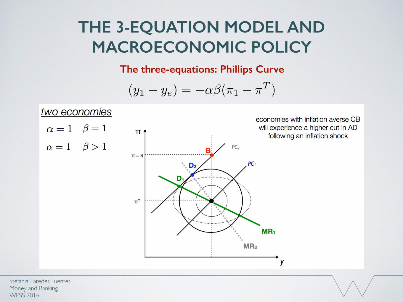
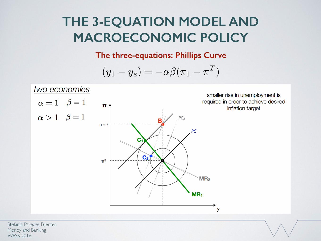
The three-equations: Phillips Curve
THE 3-EQUATION MODEL AND MACROECONOMIC POLICY
Stefania Paredes Fuentes Money and BankingWESS 2016
The three-equations: Phillips Curve
y
π
ye
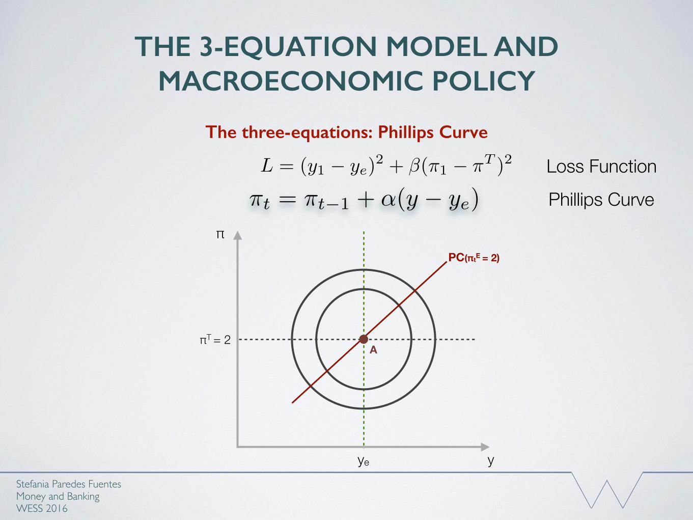
πT = 2
⇡t = ⇡t�1 + ↵(y � ye)
PC(πtE = 2)
A
L = (y1 � ye)2 + �(⇡1 � ⇡T )2 Loss Function
Phillips Curve
THE 3-EQUATION MODEL AND MACROECONOMIC POLICY
Stefania Paredes Fuentes Money and BankingWESS 2016
The three-equations: Phillips Curve
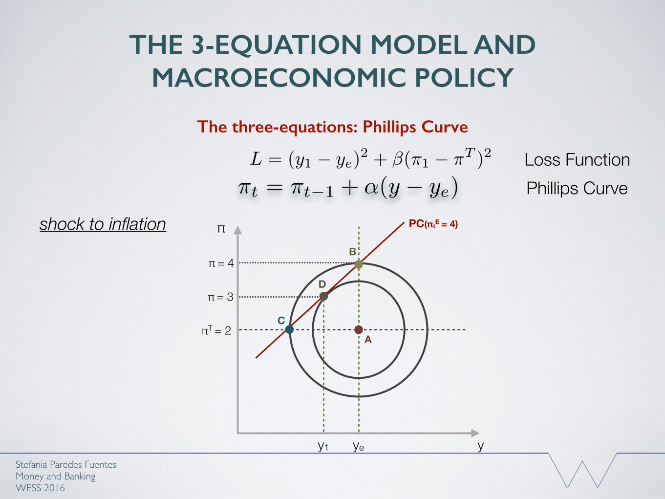
⇡t = ⇡t�1 + ↵(y � ye)L = (y1 � ye)
2 + �(⇡1 � ⇡T )2 Loss FunctionPhillips Curve
y
π
ye
πT = 2
PC(πtE = 4)
π = 4
y1
A
B
D
C
shock to inflation
π = 3
THE 3-EQUATION MODEL AND MACROECONOMIC POLICY
Stefania Paredes Fuentes Money and BankingWESS 2016
The three-equations: Phillips Curve
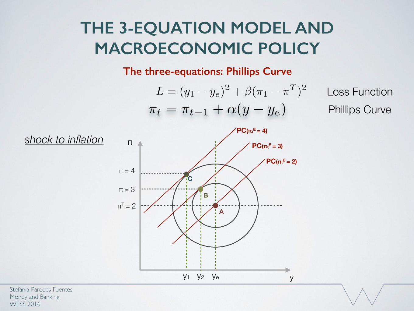
⇡t = ⇡t�1 + ↵(y � ye)L = (y1 � ye)
2 + �(⇡1 � ⇡T )2 Loss FunctionPhillips Curve
shock to inflation
y
π
ye
πT = 2
PC(πtE = 3)
PC(πtE = 2)
PC(πtE = 4)
π = 3
π = 4
y1
A
B
C
y2
THE 3-EQUATION MODEL AND MACROECONOMIC POLICY
Stefania Paredes Fuentes Money and BankingWESS 2016
The three-equations: Monetary Rule
⇡t = ⇡t�1 + ↵(y � ye)L = (y1 � ye)
2 + �(⇡1 � ⇡T )2 Loss FunctionPhillips Curve
y
π
ye
πT = 2
PC(πtE = 3)
PC(πtE = 2)
PC(πtE = 4)
π = 3
π = 4
y1
A
B
C
MR
THE 3-EQUATION MODEL AND MACROECONOMIC POLICY
Stefania Paredes Fuentes Money and BankingWESS 2016
The three-equations: Phillips Curve
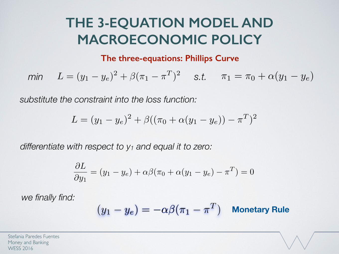
L = (y1 � ye)2 + �(⇡1 � ⇡T )2 s.t.min ⇡1 = ⇡0 + ↵(y1 � ye)
THE 3-EQUATION MODEL AND MACROECONOMIC POLICY
Stefania Paredes Fuentes Money and BankingWESS 2016
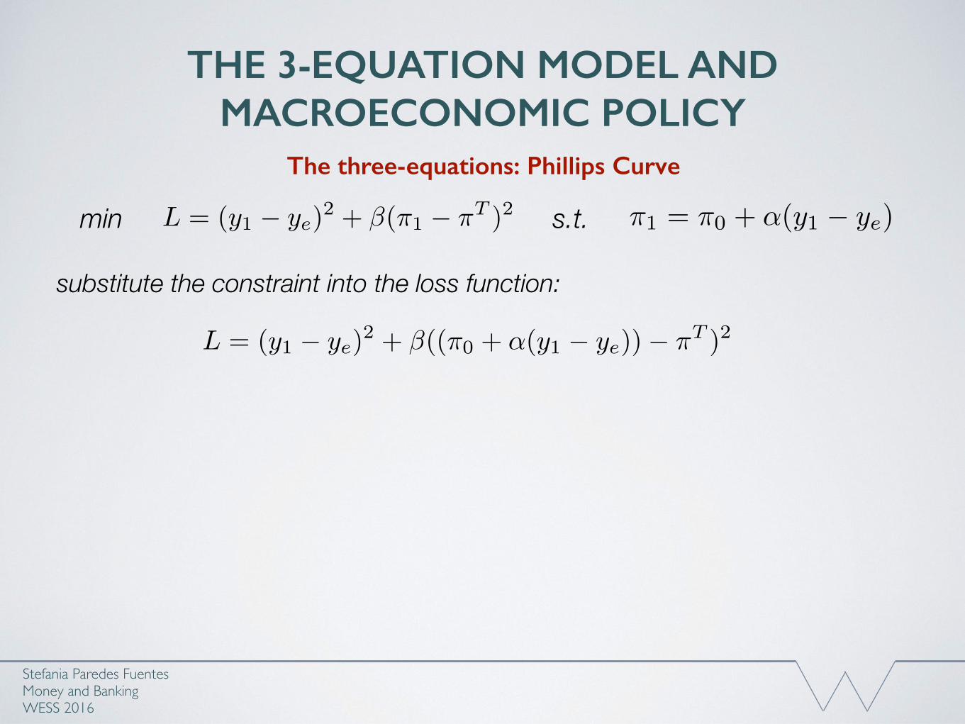
The three-equations: Phillips Curve
L = (y1 � ye)2 + �(⇡1 � ⇡T )2 s.t.min ⇡1 = ⇡0 + ↵(y1 � ye)
L = (y1 � ye)2 + �((⇡0 + ↵(y1 � ye))� ⇡T )2
substitute the constraint into the loss function:
THE 3-EQUATION MODEL AND MACROECONOMIC POLICY
Stefania Paredes Fuentes Money and BankingWESS 2016
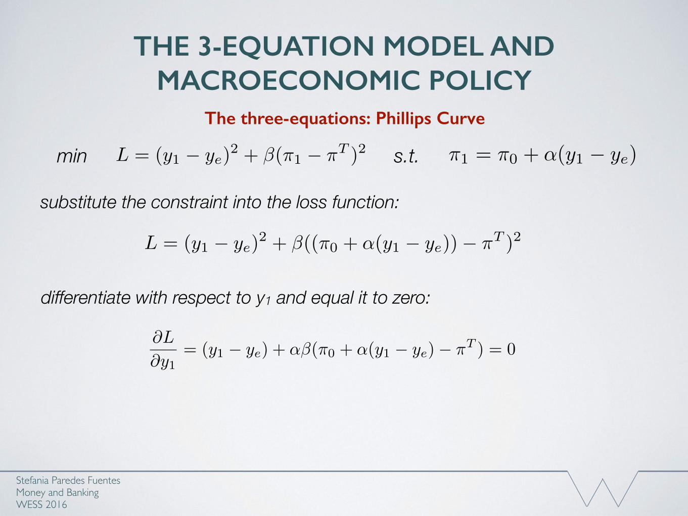
The three-equations: Phillips Curve
L = (y1 � ye)2 + �(⇡1 � ⇡T )2 s.t.min ⇡1 = ⇡0 + ↵(y1 � ye)
L = (y1 � ye)2 + �((⇡0 + ↵(y1 � ye))� ⇡T )2
substitute the constraint into the loss function:
differentiate with respect to y1 and equal it to zero:
@L
@y1= (y1 � ye) + ↵�(⇡0 + ↵(y1 � ye)� ⇡T ) = 0
THE 3-EQUATION MODEL AND MACROECONOMIC POLICY
Stefania Paredes Fuentes Money and BankingWESS 2016
The three-equations: Phillips Curve
L = (y1 � ye)2 + �(⇡1 � ⇡T )2 s.t.min ⇡1 = ⇡0 + ↵(y1 � ye)
L = (y1 � ye)2 + �((⇡0 + ↵(y1 � ye))� ⇡T )2
substitute the constraint into the loss function:
differentiate with respect to y1 and equal it to zero:
@L
@y1= (y1 � ye) + ↵�(⇡0 + ↵(y1 � ye)� ⇡T ) = 0
we finally find:(y1 � ye) = �↵�(⇡1 � ⇡T ) Monetary Rule
THE 3-EQUATION MODEL AND MACROECONOMIC POLICY
Stefania Paredes Fuentes Money and BankingWESS 2016
The three-equations: Phillips Curve
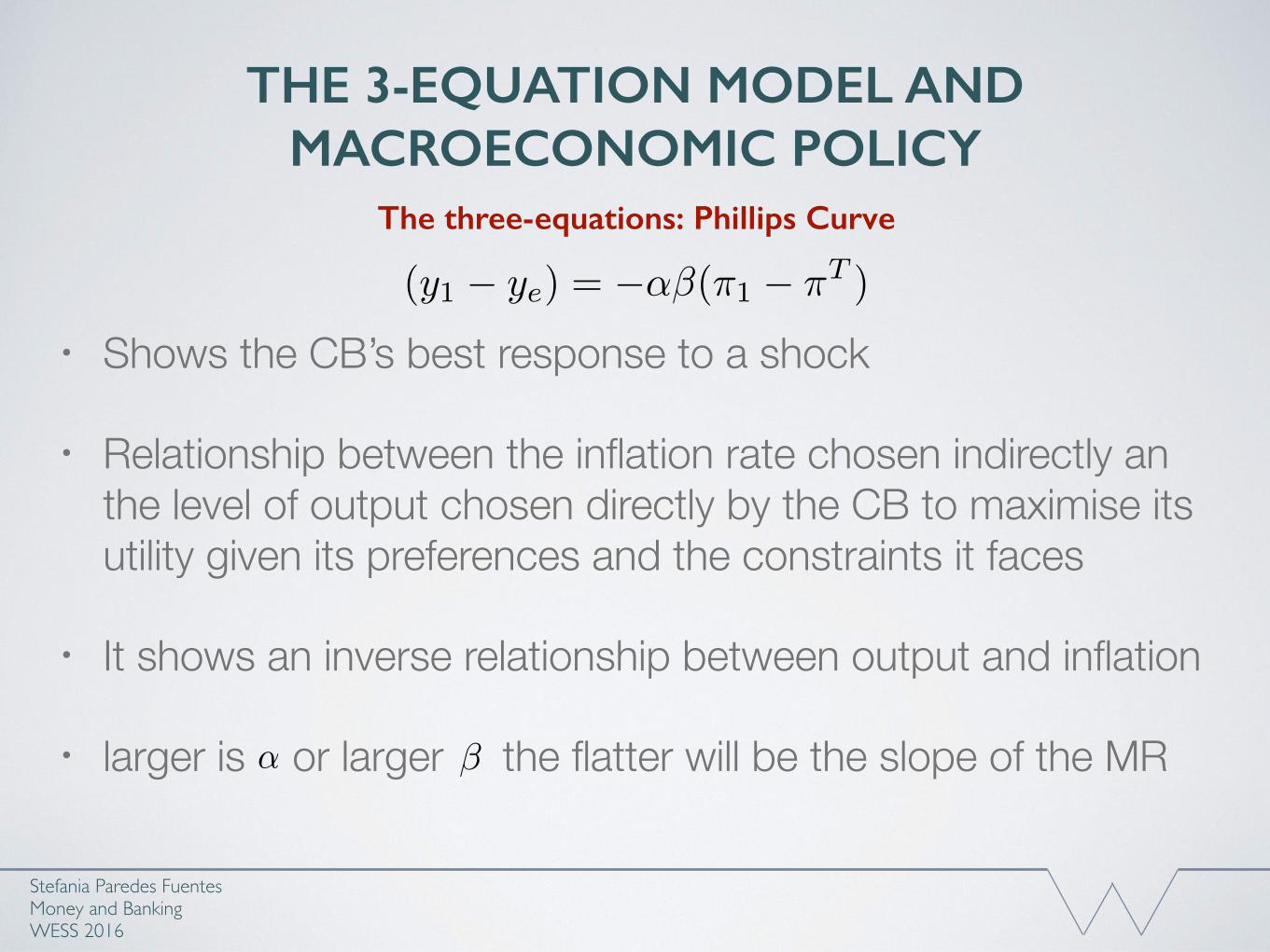
• Shows the CB’s best response to a shock
• Relationship between the inflation rate chosen indirectly an the level of output chosen directly by the CB to maximise its utility given its preferences and the constraints it faces
• It shows an inverse relationship between output and inflation
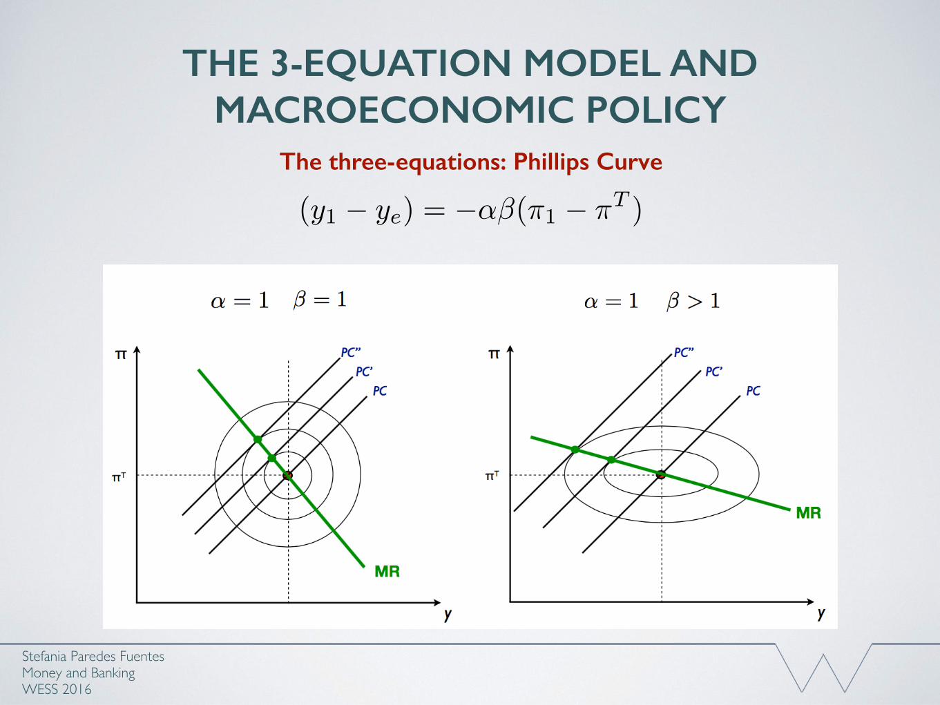
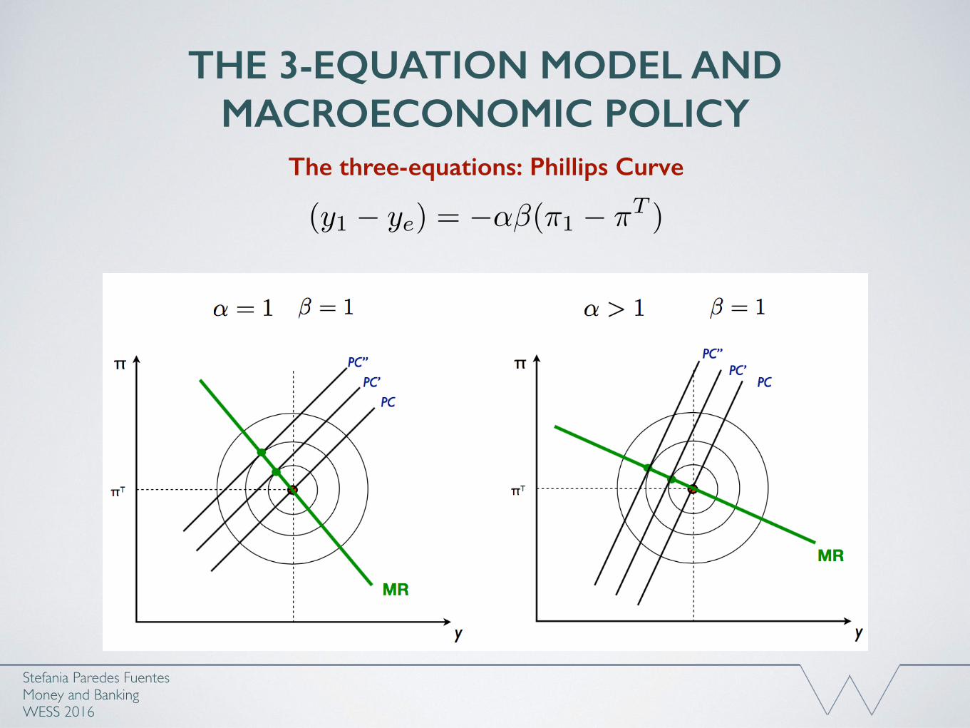
• larger is or larger the flatter will be the slope of the MR
(y1 � ye) = �↵�(⇡1 � ⇡T )
↵ �
THE 3-EQUATION MODEL AND MACROECONOMIC POLICY
Stefania Paredes Fuentes Money and BankingWESS 2016
The three-equations: Phillips Curve
(y1 � ye) = �↵�(⇡1 � ⇡T )
THE 3-EQUATION MODEL AND MACROECONOMIC POLICY
Stefania Paredes Fuentes Money and BankingWESS 2016
The three-equations: Phillips Curve
(y1 � ye) = �↵�(⇡1 � ⇡T )
THE 3-EQUATION MODEL AND MACROECONOMIC POLICY
Stefania Paredes Fuentes Money and BankingWESS 2016
The three-equations: Phillips Curve
(y1 � ye) = �↵�(⇡1 � ⇡T )
THE 3-EQUATION MODEL AND MACROECONOMIC POLICY
Stefania Paredes Fuentes Money and BankingWESS 2016
The three-equations: Phillips Curve
(y1 � ye) = �↵�(⇡1 � ⇡T )
• Active rule-based MP: best response r to achieve inflation target
• Deriving the Monetary Rule (MR):
(1) Define the central bank’s preferences in terms of deviations from inflation target and equilibrium output.
(2) Define the central bank’s constraints from the supply side, ie the Phillips Curve (PC)
(3) Derive the best response monetary rule in the output-inflation space, which gives the MR curve.
(4) Once the optimal output-inflation combination is determined using the MR, the central bank uses the IS curve to implement its choice (by setting the interest rate)
THE 3-EQUATION MODEL AND MACROECONOMIC POLICY
Stefania Paredes Fuentes Money and BankingWESS 2016
The 3-Equations
THE 3-EQUATION MODEL AND MACROECONOMIC POLICY
• IS curve (equilibrium in the goods market)
• PC curve (unemployment-inflation relationship)
• MR curve (how the CB responds to shocks)
Stefania Paredes Fuentes Money and BankingWESS 2016
The 3 Equations
THE 3-EQUATION MODEL AND MACROECONOMIC POLICY
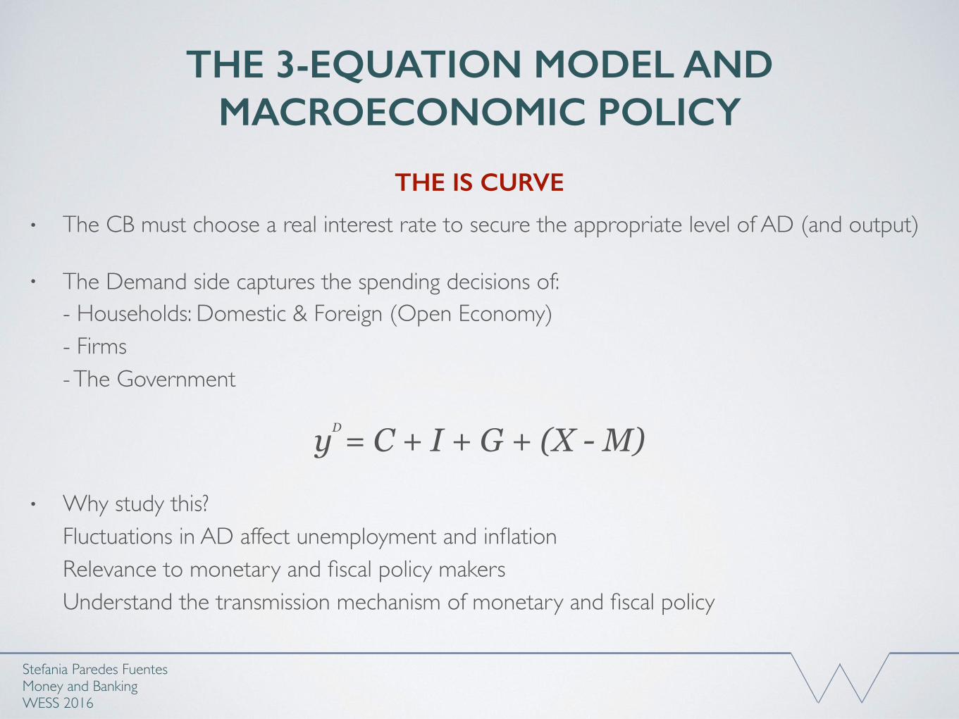
• The CB must choose a real interest rate to secure the appropriate level of AD (and output)
• The Demand side captures the spending decisions of:- Households: Domestic & Foreign (Open Economy) - Firms - The Government
yD = C + I + G + (X - M)
• Why study this?Fluctuations in AD affect unemployment and inflation Relevance to monetary and fiscal policy makersUnderstand the transmission mechanism of monetary and fiscal policy
Stefania Paredes Fuentes Money and BankingWESS 2016
THE IS CURVE
THE 3-EQUATION MODEL AND MACROECONOMIC POLICY
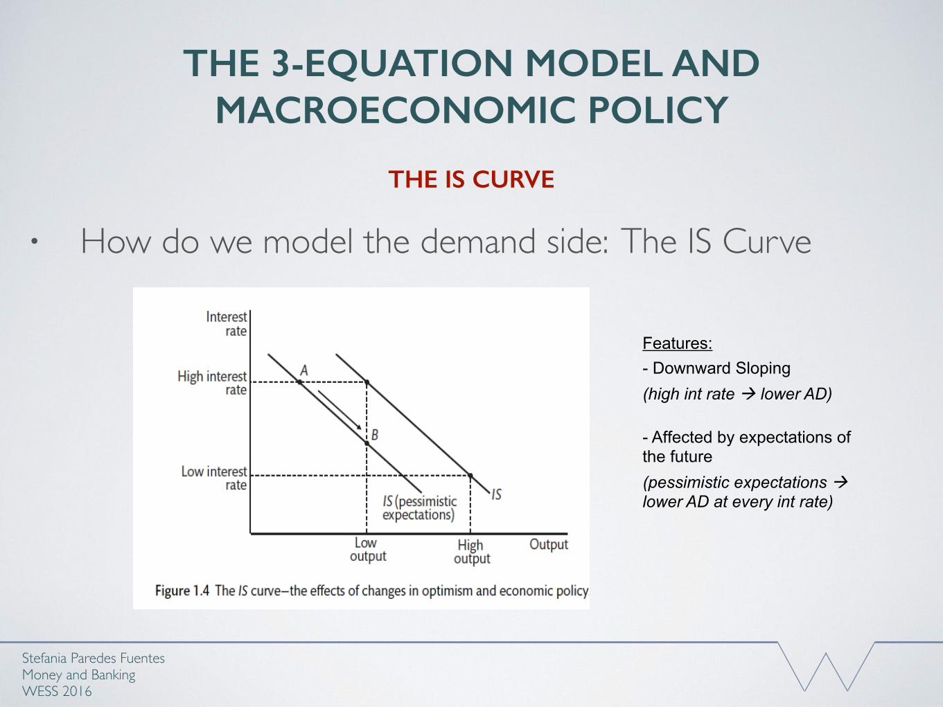
• How do we model the demand side: The IS Curve
Stefania Paredes Fuentes Money and BankingWESS 2016
THE IS CURVE
Features:- Downward Sloping(high int rate à lower AD)
- Affected by expectations of the future(pessimistic expectations àlower AD at every int rate)
THE 3-EQUATION MODEL AND MACROECONOMIC POLICY
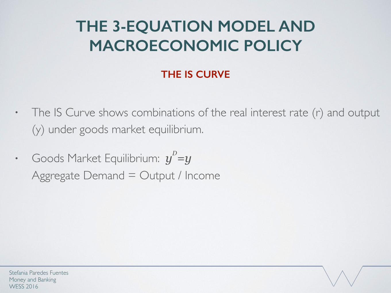
• The IS Curve shows combinations of the real interest rate (r) and output (y) under goods market equilibrium.
• Goods Market Equilibrium: yD=yAggregate Demand = Output / Income
Stefania Paredes Fuentes Money and BankingWESS 2016
THE IS CURVE
THE 3-EQUATION MODEL AND MACROECONOMIC POLICY
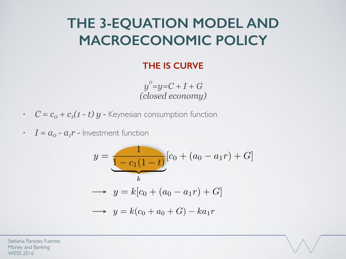
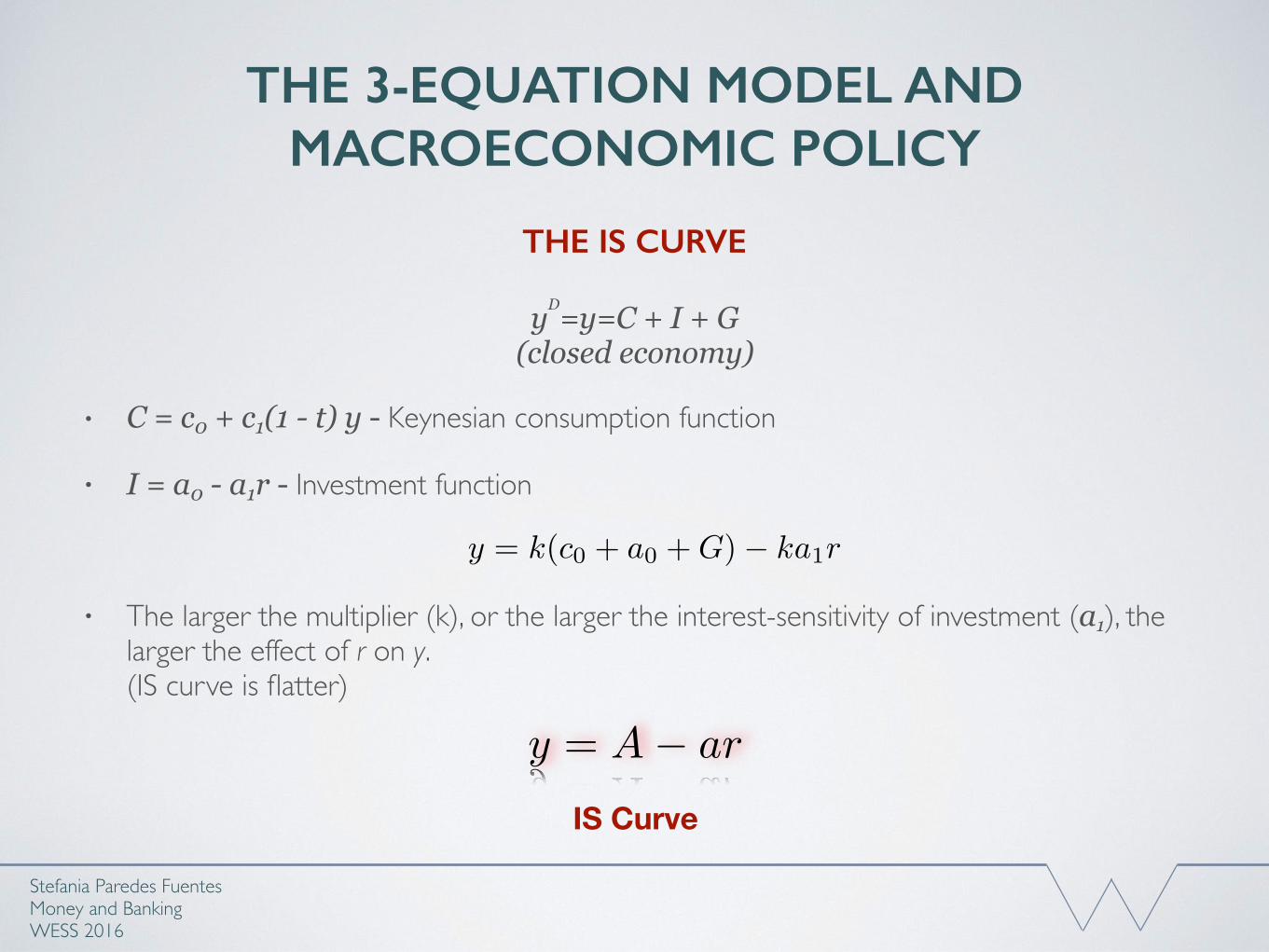
yD=y=C + I + G (closed economy)
• C = c0 + c1(1 - t) y - Keynesian consumption function
• I = a0 - a1r - Investment function
Stefania Paredes Fuentes Money and BankingWESS 2016
THE IS CURVE
y =1
1� c1(1� t)| {z }k
[c0 + (a0 � a1r) +G]
y = k[c0 + (a0 � a1r) +G]
y = k(c0 + a0 +G)� ka1r
THE 3-EQUATION MODEL AND MACROECONOMIC POLICY
yD=y=C + I + G (closed economy)
• C = c0 + c1(1 - t) y - Keynesian consumption function
• I = a0 - a1r - Investment function
• The larger the multiplier (k), or the larger the interest-sensitivity of investment (a1), the larger the effect of r on y. (IS curve is flatter)
Stefania Paredes Fuentes Money and BankingWESS 2016
THE IS CURVE
y = k(c0 + a0 +G)� ka1r
y = A� ar
IS Curve
THE 3-EQUATION MODEL AND MACROECONOMIC POLICY
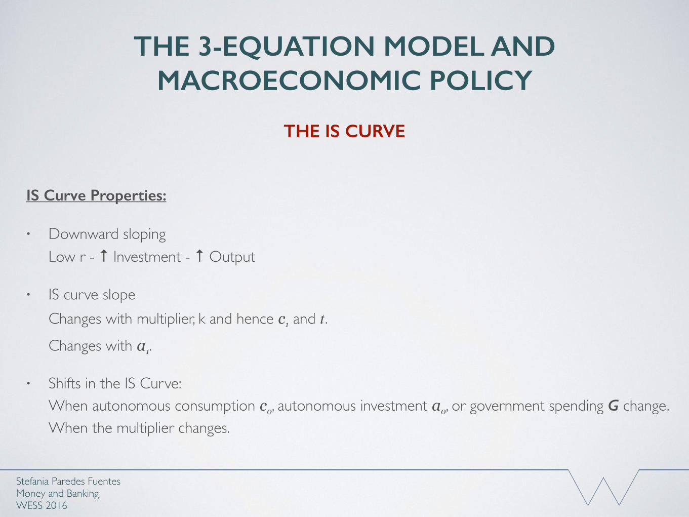
IS Curve Properties:
• Downward slopingLow r - ↑ Investment - ↑ Output
• IS curve slope Changes with multiplier, k and hence c1 and 𝑡.Changes with a1.
• Shifts in the IS Curve: When autonomous consumption c0, autonomous investment a0, or government spending G change.When the multiplier changes.
Stefania Paredes Fuentes Money and BankingWESS 2016
THE IS CURVE
THE 3-EQUATION MODEL AND MACROECONOMIC POLICY
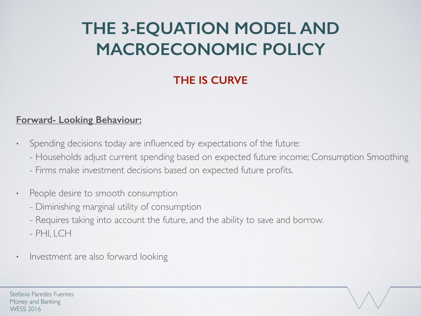
Forward- Looking Behaviour:
• Spending decisions today are influenced by expectations of the future:- Households adjust current spending based on expected future income; Consumption Smoothing- Firms make investment decisions based on expected future profits.
• People desire to smooth consumption - Diminishing marginal utility of consumption - Requires taking into account the future, and the ability to save and borrow.- PHI, LCH
• Investment are also forward looking
Stefania Paredes Fuentes Money and BankingWESS 2016
THE IS CURVE
THE 3-EQUATION MODEL AND MACROECONOMIC POLICY
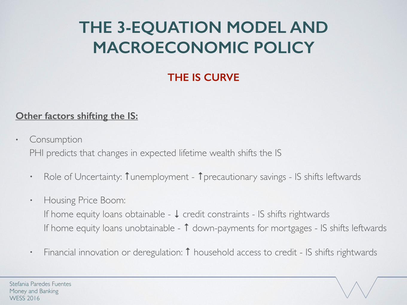
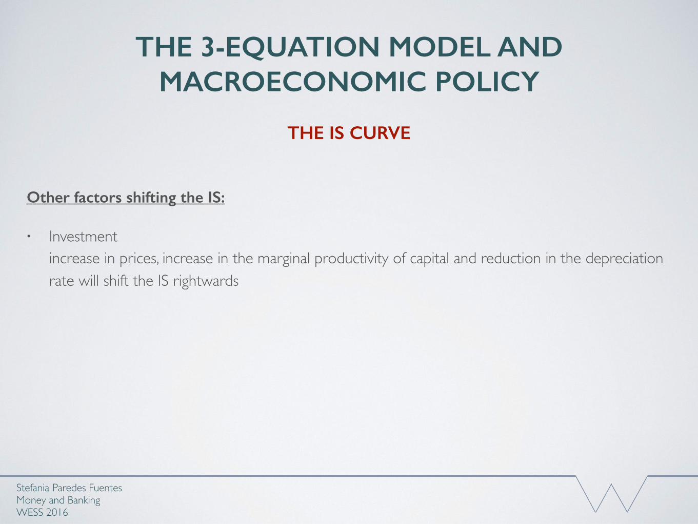
Other factors shifting the IS:
• Consumption PHI predicts that changes in expected lifetime wealth shifts the IS
• Role of Uncertainty: ↑unemployment - ↑precautionary savings - IS shifts leftwards
• Housing Price Boom: If home equity loans obtainable - ↓ credit constraints - IS shifts rightwardsIf home equity loans unobtainable - ↑ down-payments for mortgages - IS shifts leftwards
• Financial innovation or deregulation: ↑ household access to credit - IS shifts rightwards
Stefania Paredes Fuentes Money and BankingWESS 2016
THE IS CURVE
THE 3-EQUATION MODEL AND MACROECONOMIC POLICY
Other factors shifting the IS:
• Investment increase in prices, increase in the marginal productivity of capital and reduction in the depreciation rate will shift the IS rightwards
Stefania Paredes Fuentes Money and BankingWESS 2016
THE IS CURVE
THE 3-EQUATION MODEL AND MACROECONOMIC POLICY
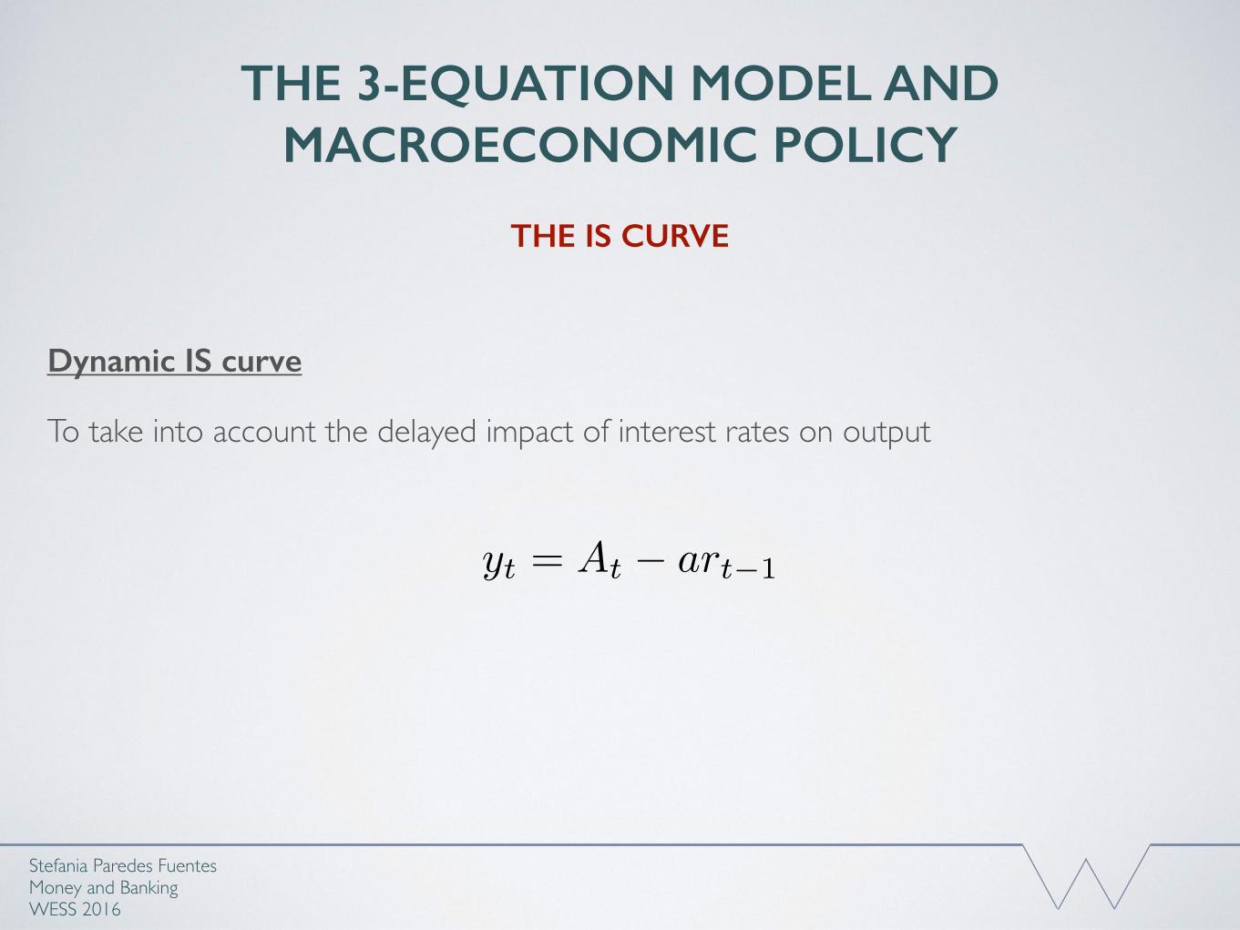
Dynamic IS curve
To take into account the delayed impact of interest rates on output
Stefania Paredes Fuentes Money and BankingWESS 2016
THE IS CURVE
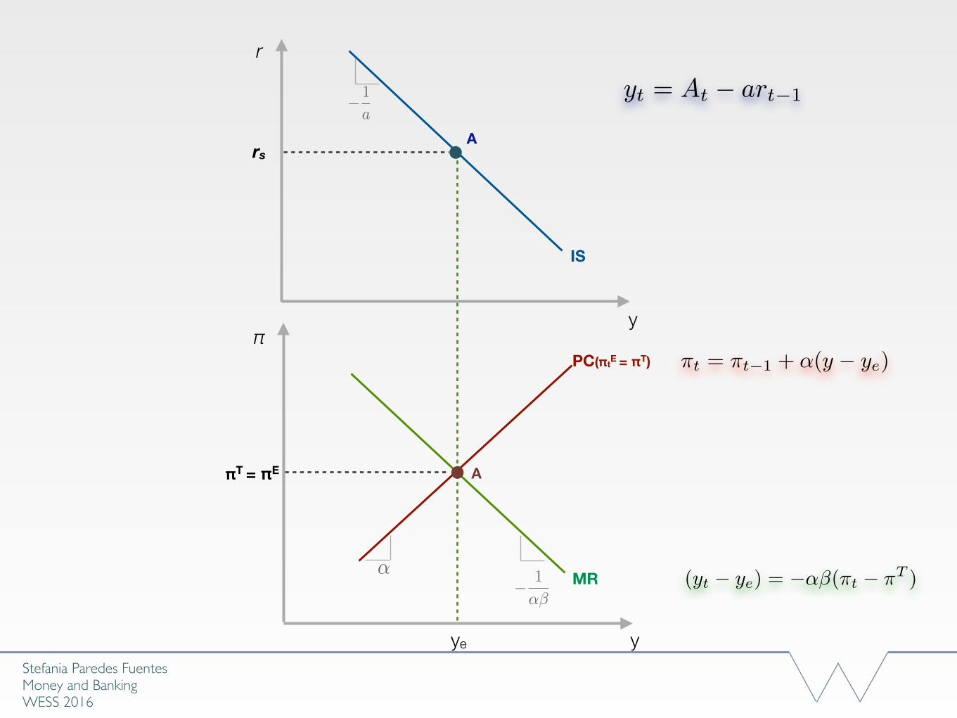
yt = At � art�1
THE 3-EQUATION MODEL AND MACROECONOMIC POLICY
Stefania Paredes Fuentes Money and BankingWESS 2016
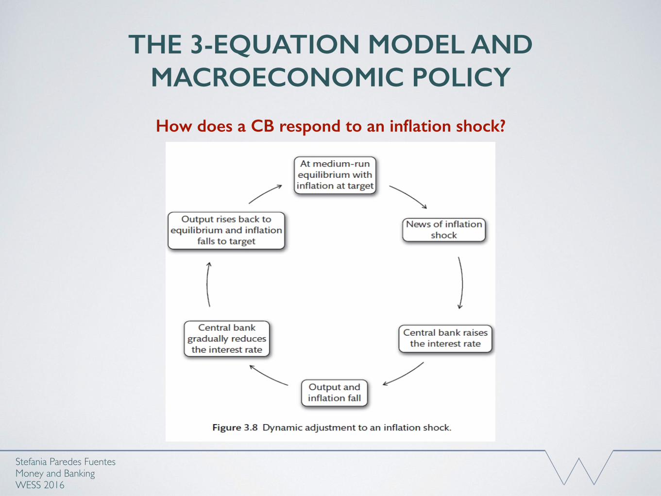
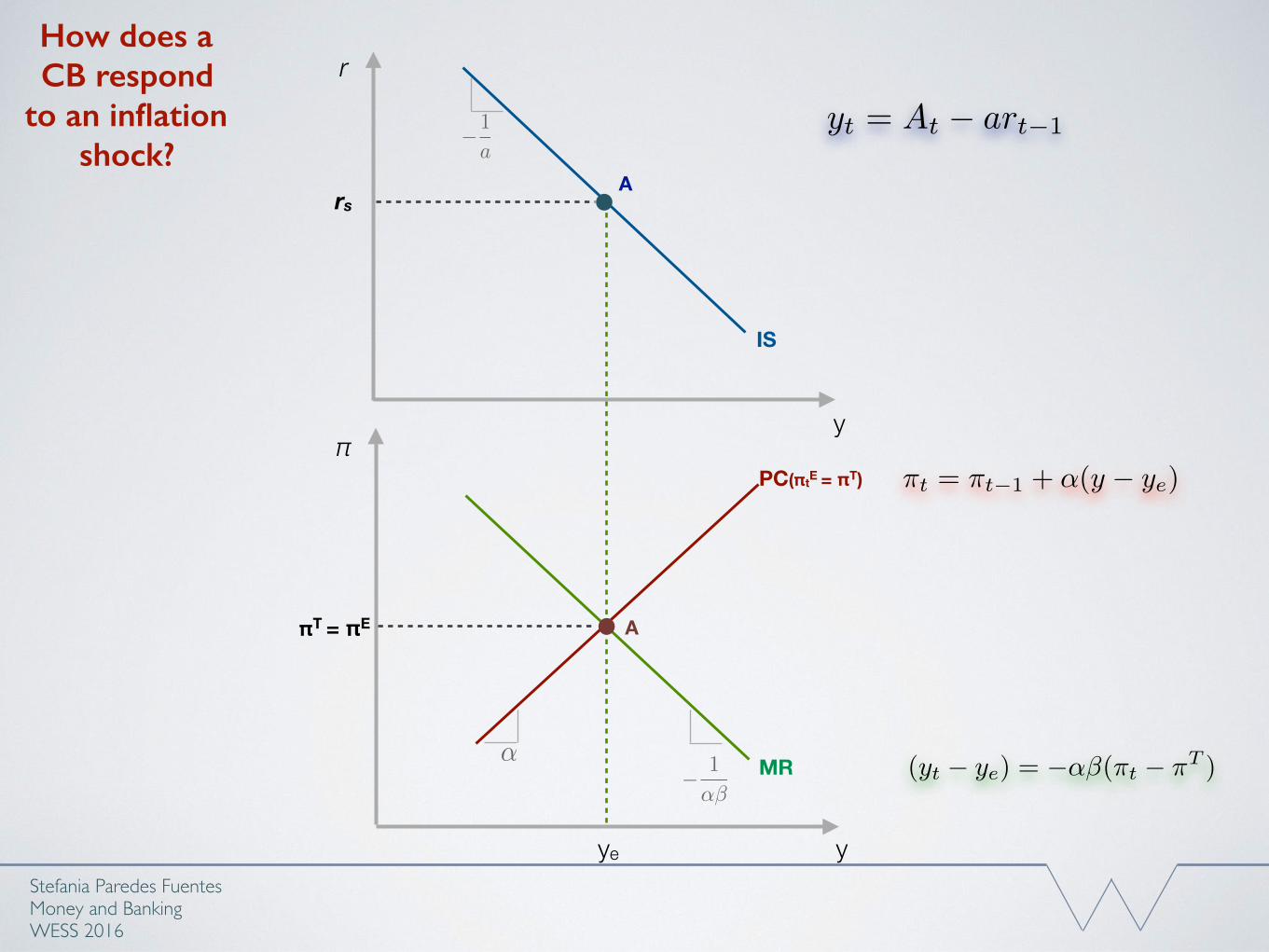
How does a CB respond to an inflation shock?
Stefania Paredes Fuentes Money and BankingWESS 2016
How does a CB respond
to an inflation shock?
y
π
ye
πT = πE
PC(πtE = πT)
A
y
rs
IS
A
r
MR
�1
a
� 1
↵�
↵
yt = At � art�1
⇡t = ⇡t�1 + ↵(y � ye)
(yt � ye) = �↵�(⇡t � ⇡T )
Stefania Paredes Fuentes Money and BankingWESS 2016
How does a CB respond
to an inflation shock?
y
π
ye
πT
PC
A
y
r
IS
A
r
PC’
inflation shock
Long run equilibrium
B’π0
THE 3-EQUATION MODEL AND MACROECONOMIC POLICY
Stefania Paredes Fuentes Money and BankingWESS 2016
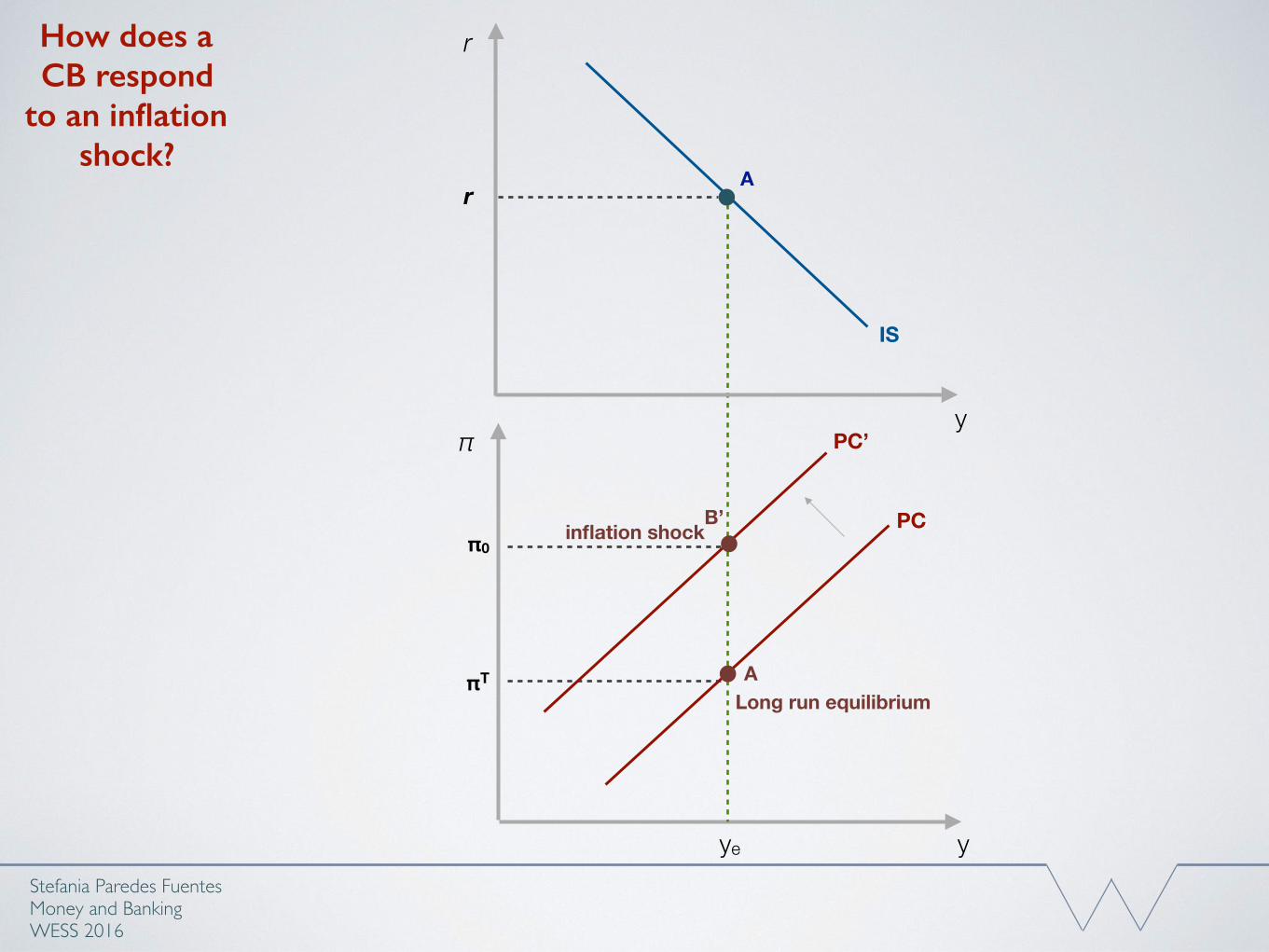
How does a CB respond to an inflation shock?
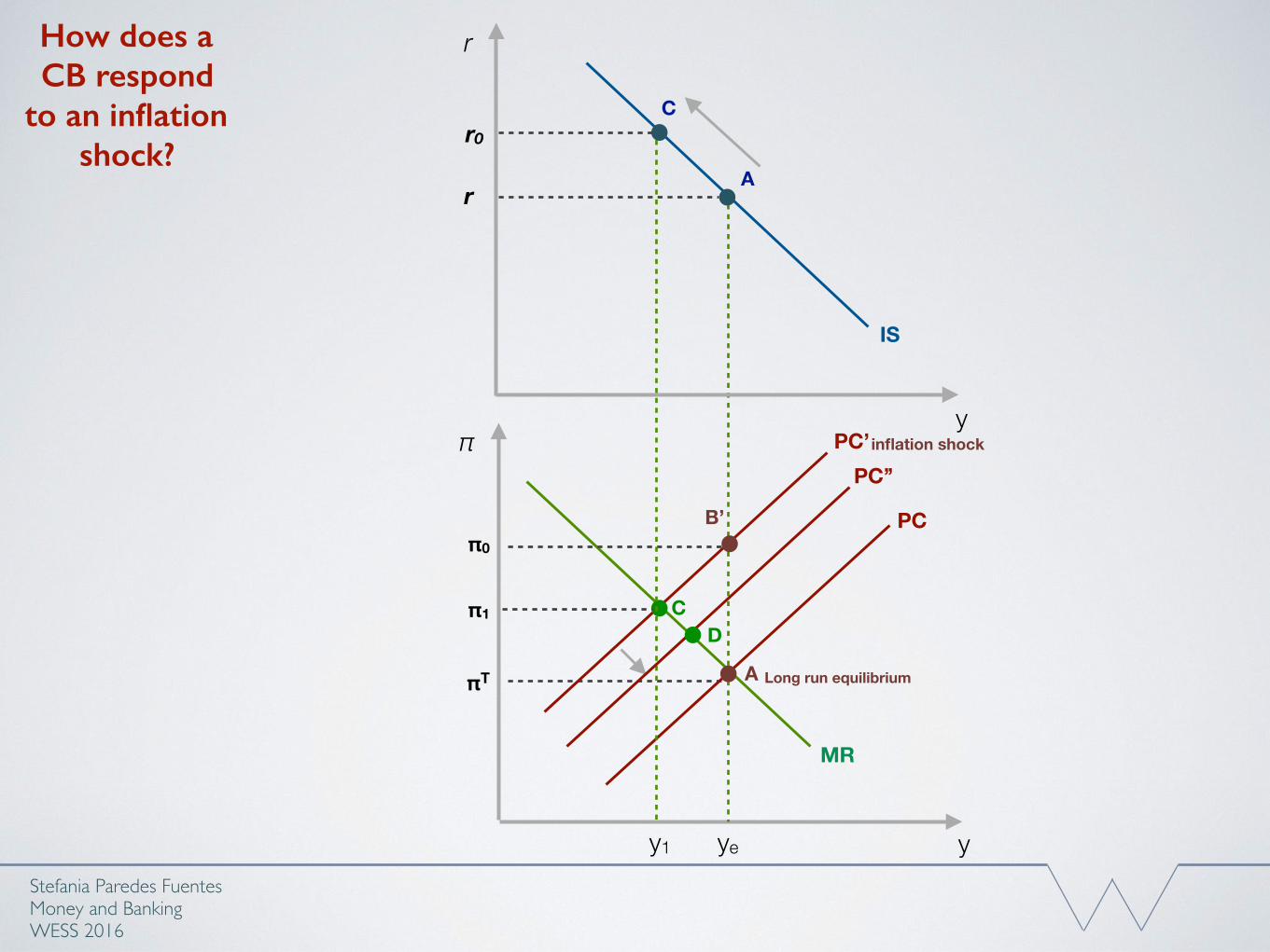
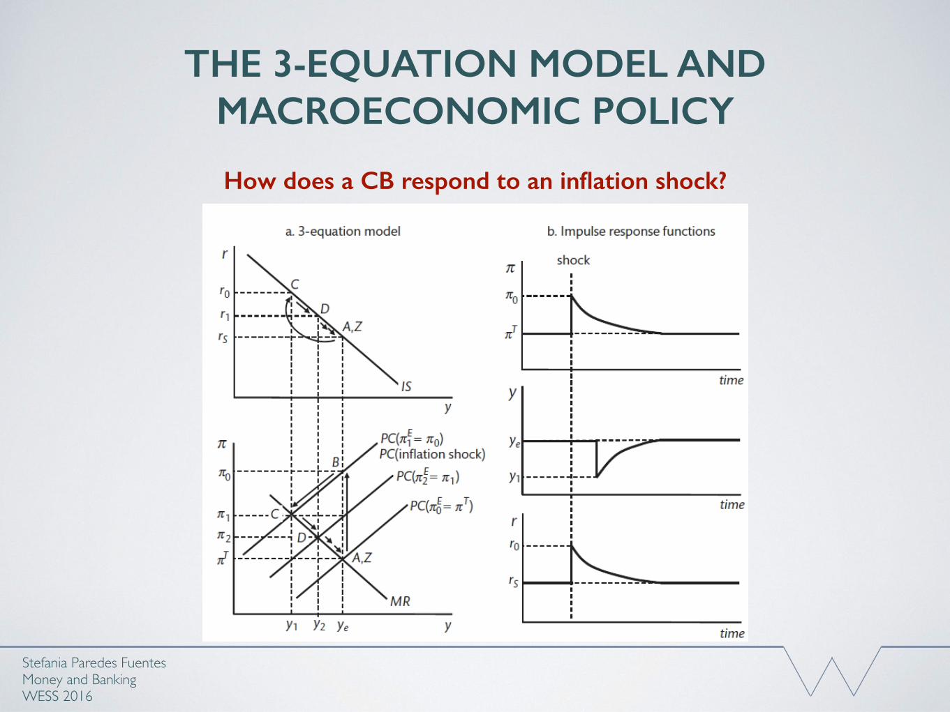
Period 0: • The economy is initially at point ‘A’ (the Bliss point) • Inflation shock: PC shifts upwards (Economy moves to point ‘B’) • The CB forecasts PC for the next period, which is PC (𝜋1𝐸=𝜋0) • The CB chooses position on this PC which minimises its loss (point ‘C’ where
the MR = PC); To achieve this, 𝑟0 is set (see IS curve) • 𝑟 affects 𝑦 with a 1-period lag, so the economy ends with (‘𝜋0, 𝑦e and 𝑟0’).
Stefania Paredes Fuentes Money and BankingWESS 2016
How does a CB respond
to an inflation shock?
y
π
ye
πT
PC
A
y
r
IS
A
r
PC’inflation shock
Long run equilibrium
B’π0
C
MR
π1
Cr0
THE 3-EQUATION MODEL AND MACROECONOMIC POLICY
Stefania Paredes Fuentes Money and BankingWESS 2016
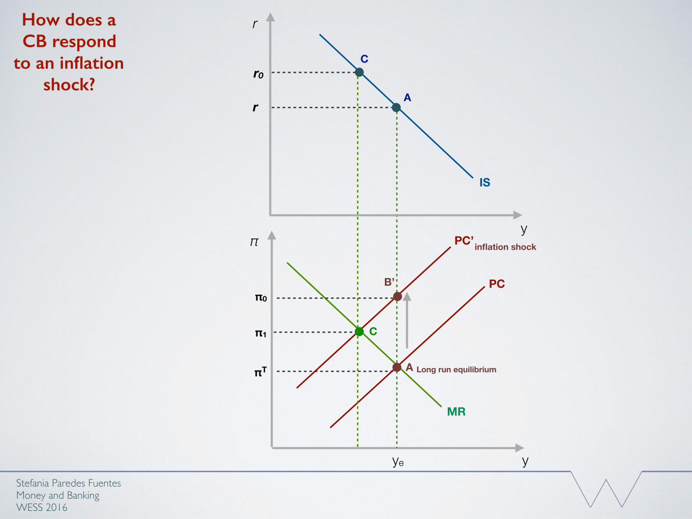
How does a CB respond to an inflation shock?
Period 1: The higher 𝑟0 reduces output below equilibrium to 𝑦1 by ↓ Investment (Economy moves to
point ‘C’) Again, the CB forecasts PC for period 2, i.e. PC (𝜋2𝐸=𝜋1); Note that the PC shifts as 𝜋𝐸 is
updated. The optimal point as given by the MR is now ‘D’; To achieve this, 𝑟0 is reduced to 𝑟1.
Similarly, the economy ends with (‘𝜋1, 𝑦1 and 𝑟1’).
Stefania Paredes Fuentes Money and BankingWESS 2016
How does a CB respond
to an inflation shock?
y
π
ye
πT
PC
A
y
r
IS
A
r
PC’inflation shock
Long run equilibrium
B’π0
C
MR
π1
Cr0
y1
PC’’
D
THE 3-EQUATION MODEL AND MACROECONOMIC POLICY
Stefania Paredes Fuentes Money and BankingWESS 2016
How does a CB respond to an inflation shock?
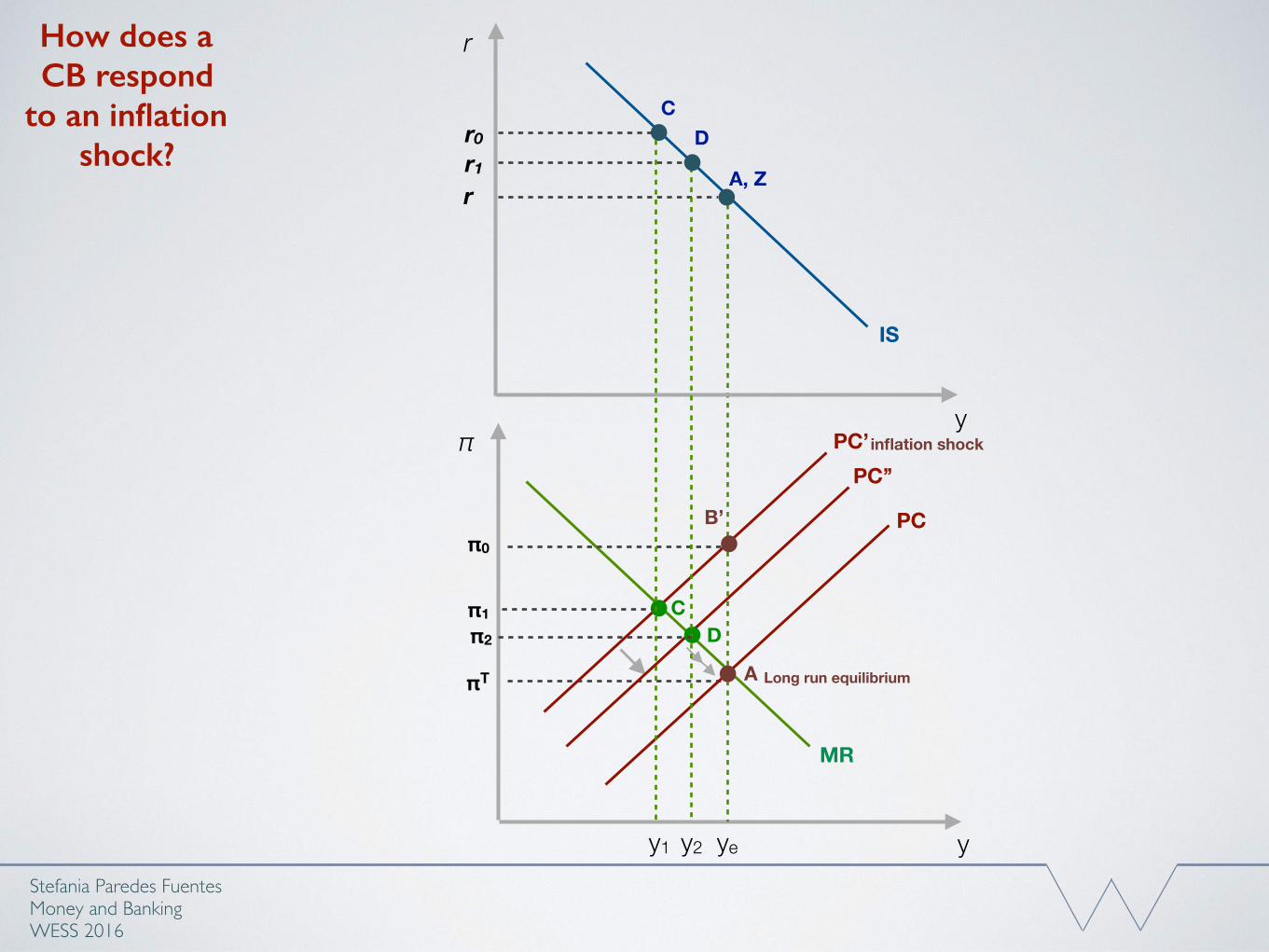
Period 2: The lower 𝑟1 increases output to 𝑦2, while inflation falls to 𝜋2 (Economy moves to point ‘D’) The same process repeats until the economy is back at its equilibrium ‘Z’ The economy moves down along MR curve: The CB gradually adjusts 𝑟1 down to 𝑟, output rises
slowly from 𝑦2 to 𝑦e and inflation eventually falls from 𝜋2 to 𝜋T.
Stefania Paredes Fuentes Money and BankingWESS 2016
How does a CB respond
to an inflation shock?
y
π
ye
πT
PC
A
y
r
IS
A, Z
r
PC’inflation shock
Long run equilibrium
B’π0
C
MR
π1
Cr0
y1
PC’’
D
y2
D
π2
r1
THE 3-EQUATION MODEL AND MACROECONOMIC POLICY
Stefania Paredes Fuentes Money and BankingWESS 2016
How does a CB respond to an inflation shock?
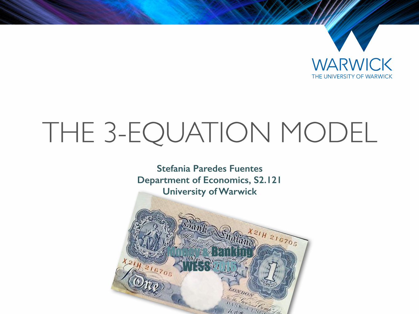
The Impulse Response Function:
It shows the time path of macroeconomic variables following a shock and the resulting policy responses.
Note that the impulse response of output only changes one period after the inflation shock. This is due to the 1 period lagged effect of 𝑟 on 𝑦.
THE 3-EQUATION MODEL AND MACROECONOMIC POLICY
Stefania Paredes Fuentes Money and BankingWESS 2016
How does a CB respond to an inflation shock?
Stefania Paredes Fuentes Money and BankingWESS 2016
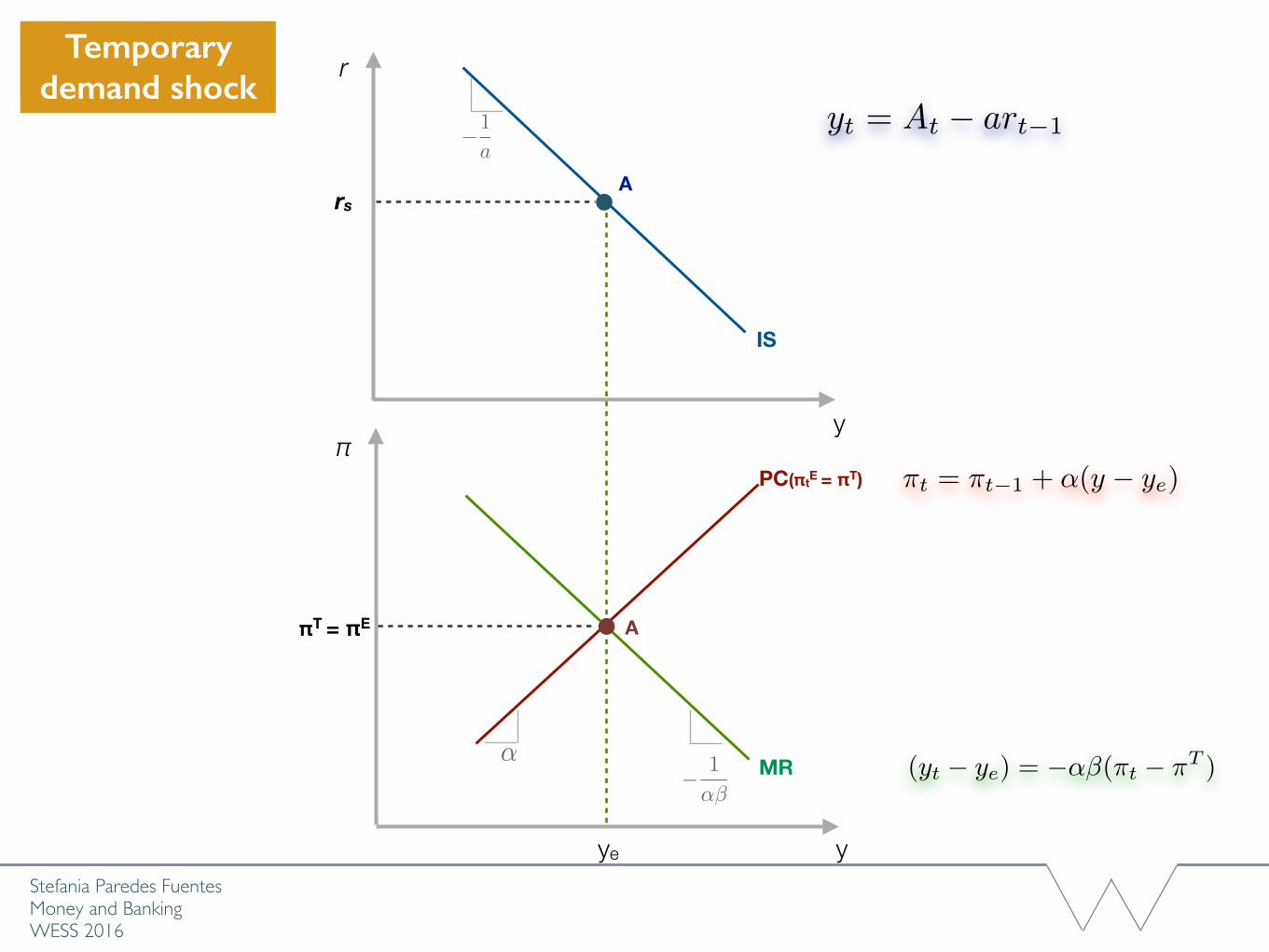
Temporary demand shock
y
π
ye
πT = πE
PC(πtE = πT)
A
y
rs
IS
A
r
MR
�1
a
� 1
↵�
↵
yt = At � art�1
⇡t = ⇡t�1 + ↵(y � ye)
(yt � ye) = �↵�(⇡t � ⇡T )
THE 3-EQUATION MODEL AND MACROECONOMIC POLICY
Stefania Paredes Fuentes Money and BankingWESS 2016
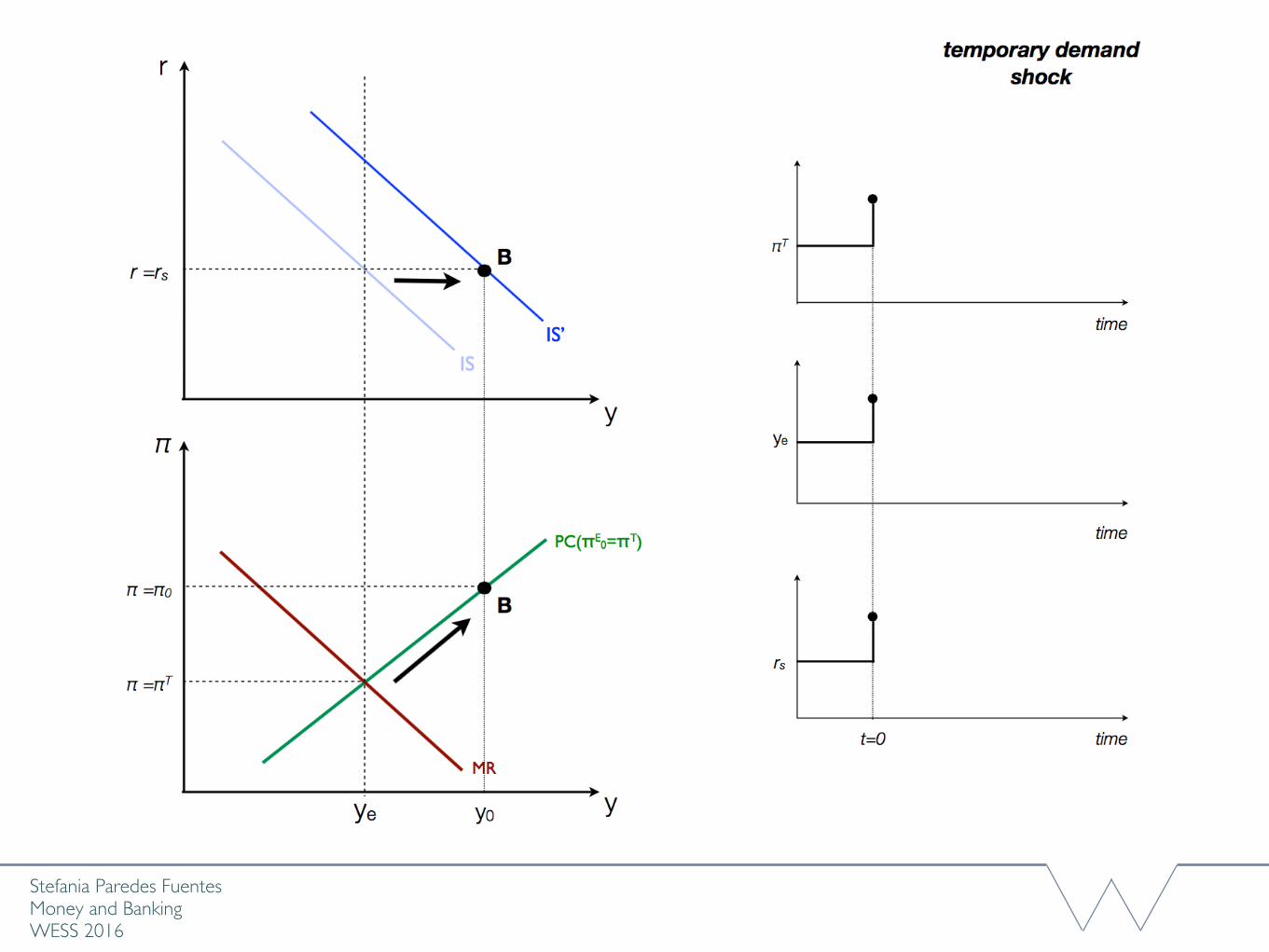
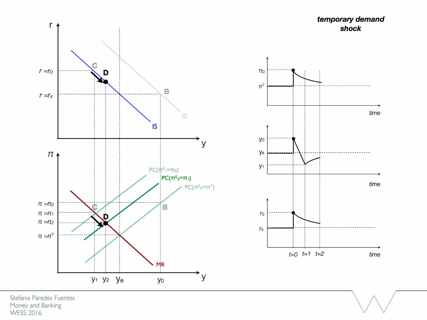
How does a CB respond to a temporary demand shock?
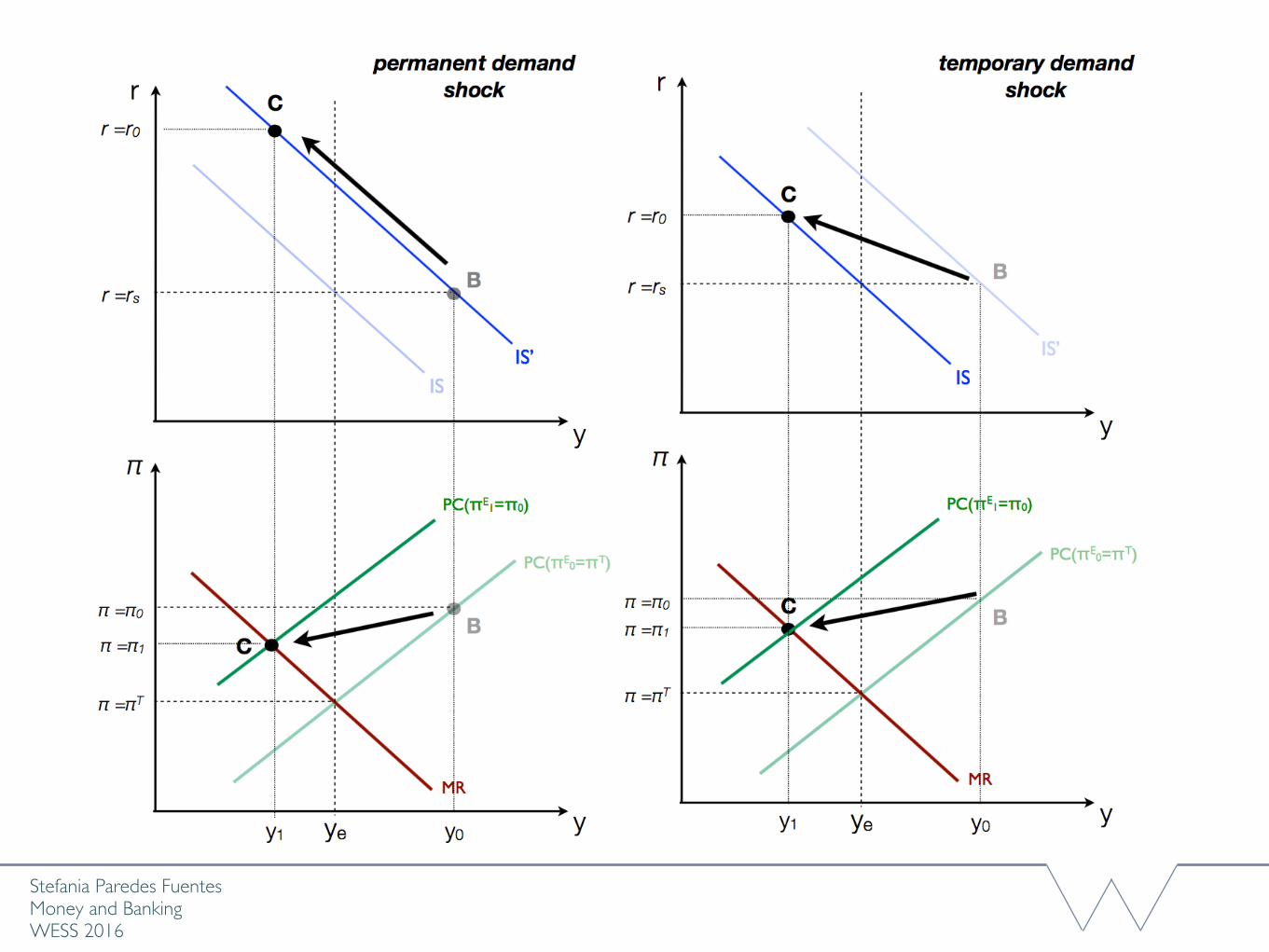
Period 0: • Temporary AD shock: IS shifts to IS’, but stays at IS’ for 1 period only.
• The economy shifts from initial point ‘A’ to point ‘B’
• The CB forecasts the PC for period 1, which is PC (𝜋1𝐸=𝜋0) • The CB knows that IS’ returns to IS at the beginning of period 1, and thus sets 𝑟0 to achieve 𝑦1 and 𝜋1, in period 1.
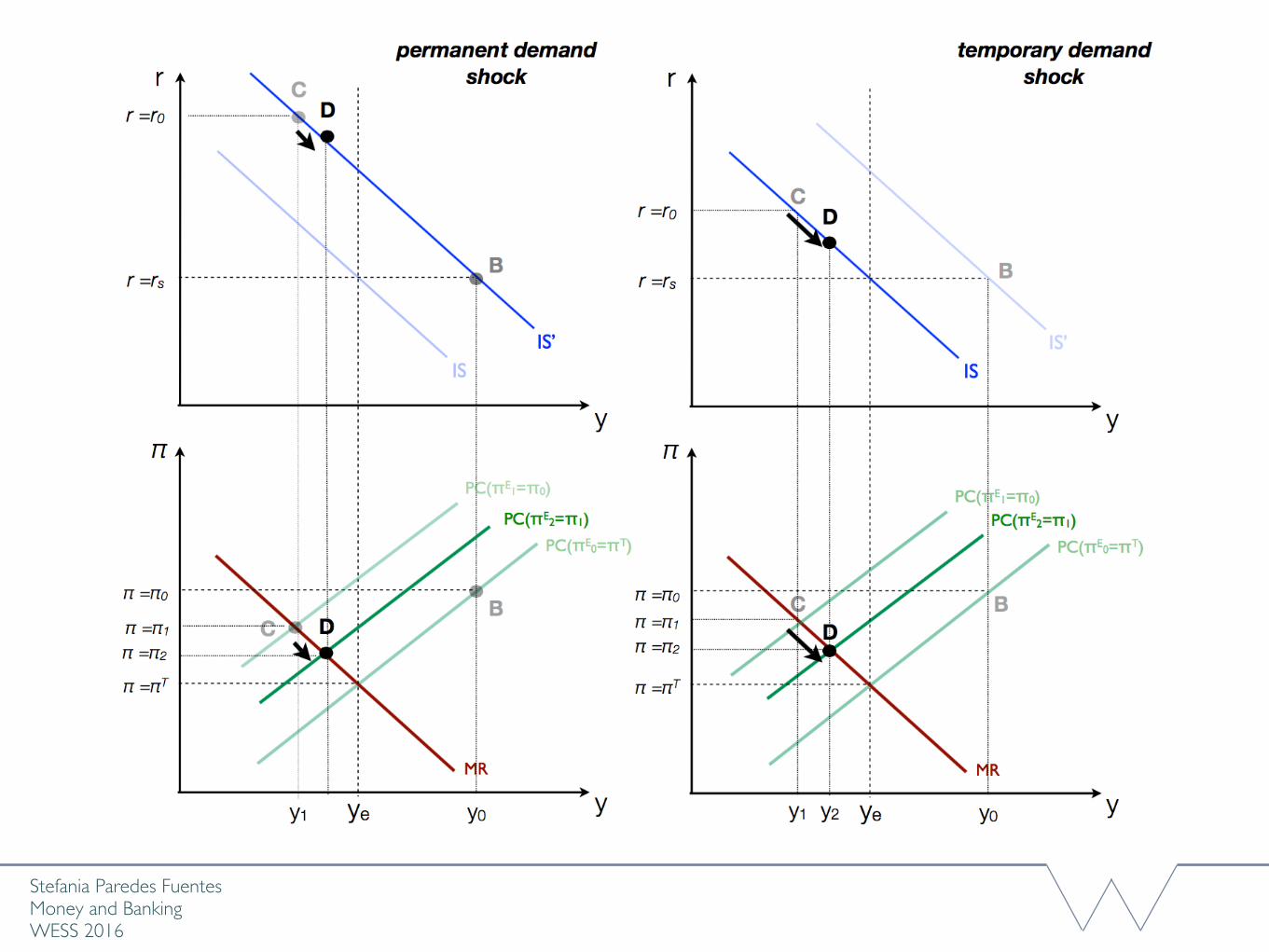
Period 1:
The higher 𝑟0 reduces π, and 𝑦 below equilibrium 𝑦e (Point ‘C’).
The CB forecasts PC for period 2 to be PC (𝜋1𝐸=𝜋0), so now, the optimal point is ‘D’; To achieve this, 𝑟0 is reduced
to 𝑟1.
Stefania Paredes Fuentes Money and BankingWESS 2016
THE 3-EQUATION MODEL AND MACROECONOMIC POLICY
Stefania Paredes Fuentes Money and BankingWESS 2016
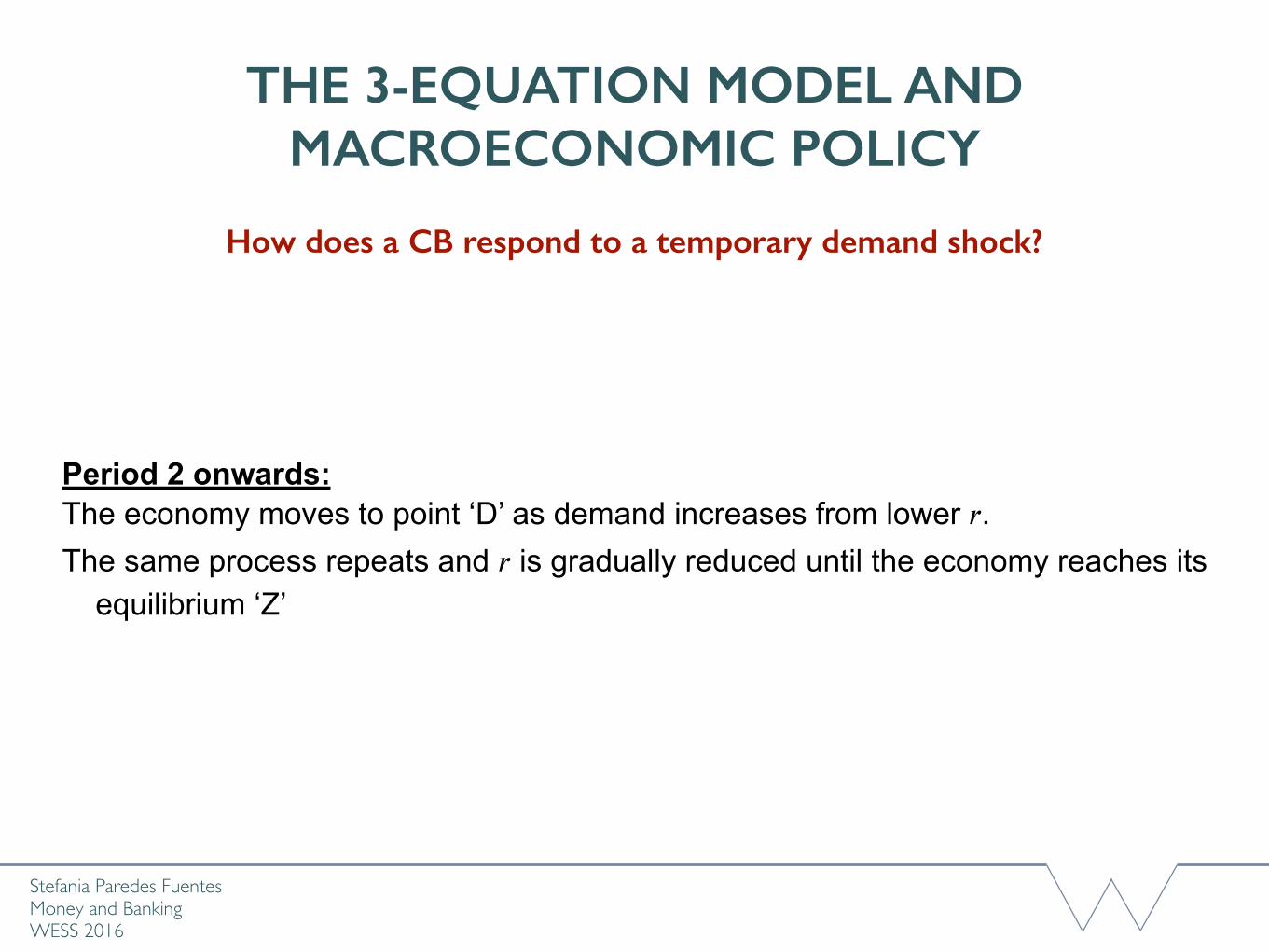
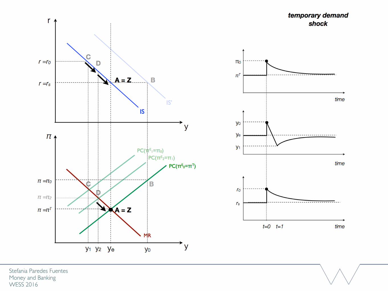
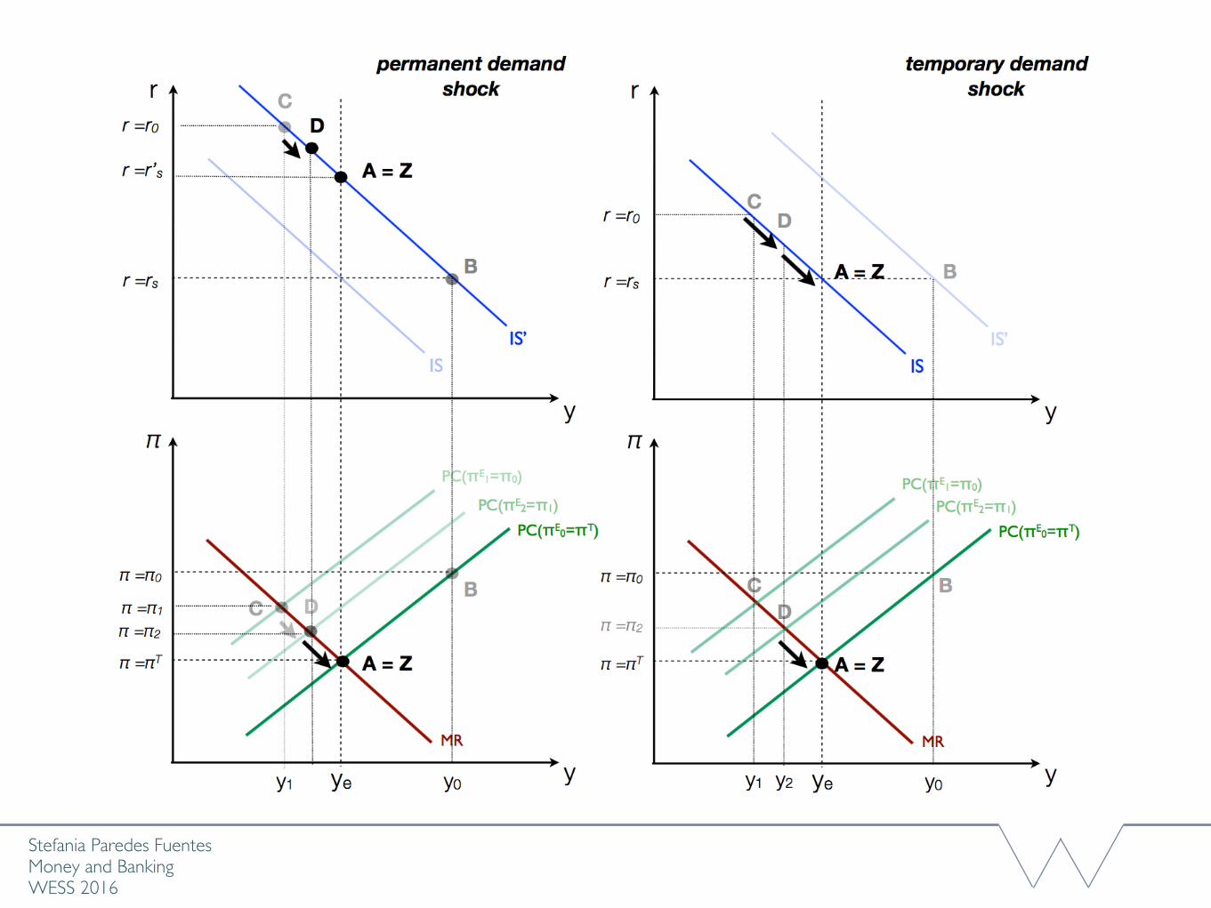
How does a CB respond to a temporary demand shock?
Period 2 onwards: The economy moves to point ‘D’ as demand increases from lower 𝑟. The same process repeats and 𝑟 is gradually reduced until the economy reaches its
equilibrium ‘Z’
Stefania Paredes Fuentes Money and BankingWESS 2016
Stefania Paredes Fuentes Money and BankingWESS 2016

THE 3-EQUATION MODEL AND MACROECONOMIC POLICY
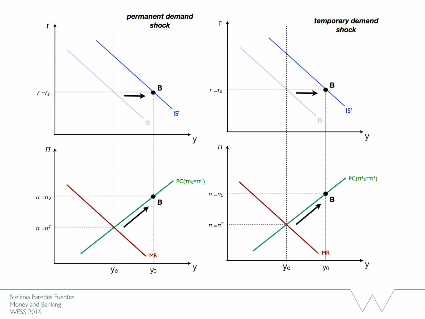
Note that the CB needs to forecast the IS and the PC curves
Forecasting the IS curve:- Is the AD shock temporary or permanent?- Vital since the persistence of shocks affects the CB’s optimal response.
Permanent shock: ISꞌ does not shift back to IS A larger increase in 𝑟 is needed compared to a temporary shock.The new equilibrium r is higher.
Stefania Paredes Fuentes Money and BankingWESS 2016
How does the CB respond to a temporary demand shock?
Stefania Paredes Fuentes Money and BankingWESS 2016
Stefania Paredes Fuentes Money and BankingWESS 2016
Stefania Paredes Fuentes Money and BankingWESS 2016
Stefania Paredes Fuentes Money and BankingWESS 2016
Stefania Paredes Fuentes Money and BankingWESS 2016
THE 3-EQUATION MODEL AND MACROECONOMIC POLICY
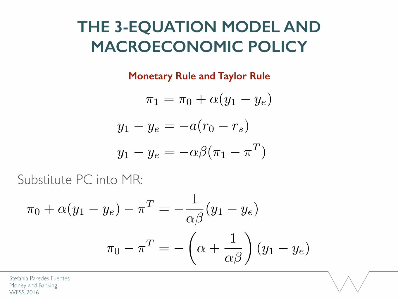
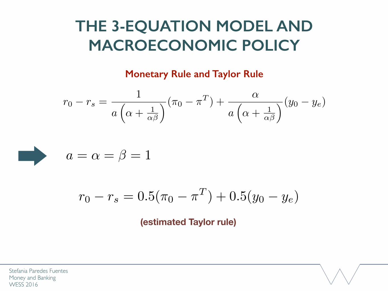
Monetary Rule and Taylor Rule
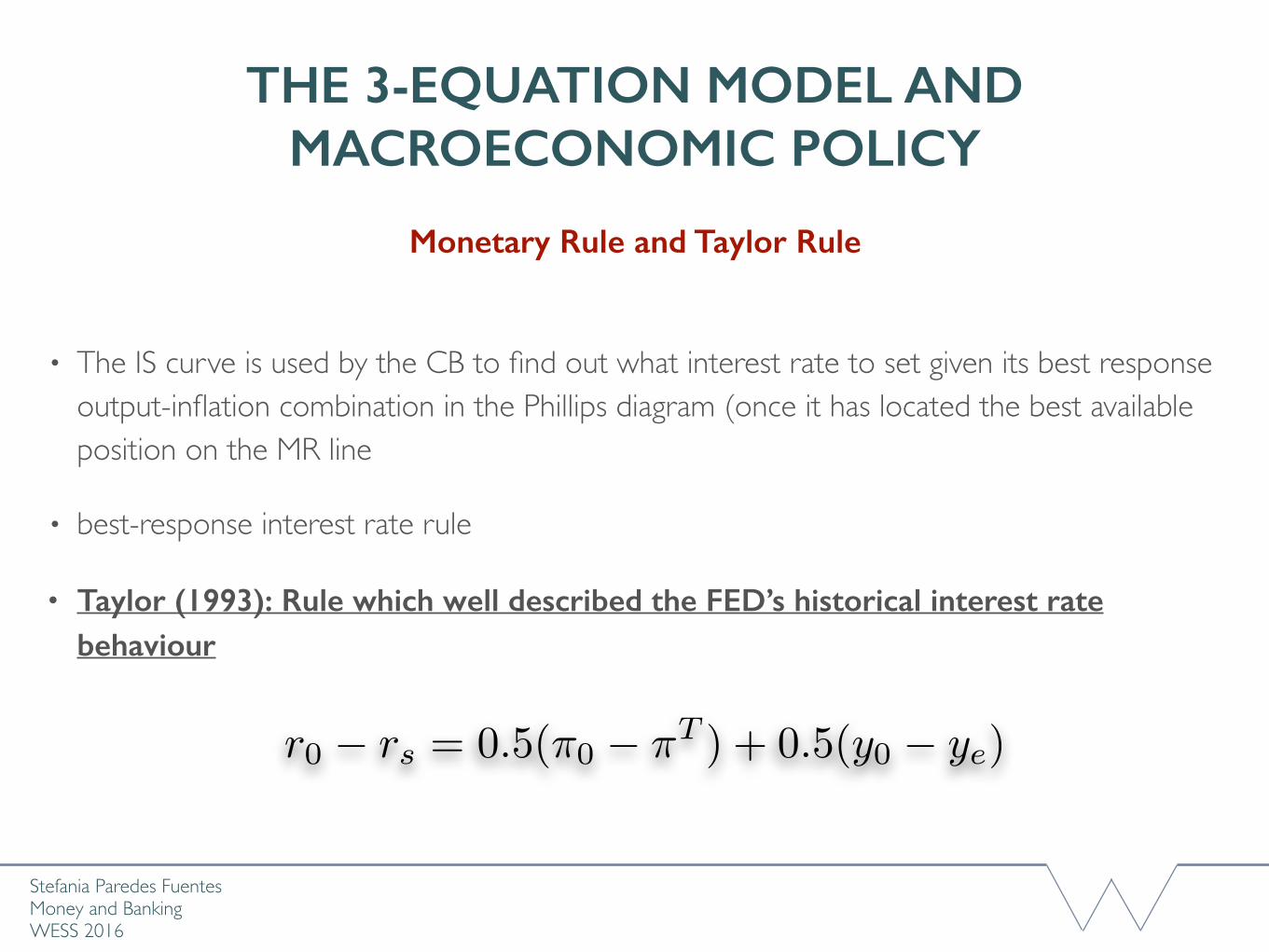
• The IS curve is used by the CB to find out what interest rate to set given its best response output-inflation combination in the Phillips diagram (once it has located the best available position on the MR line
• best-response interest rate rule
• Taylor (1993): Rule which well described the FED’s historical interest rate behaviour
r0 � rs = 0.5(⇡0 � ⇡T ) + 0.5(y0 � ye)
Stefania Paredes Fuentes Money and BankingWESS 2016
THE 3-EQUATION MODEL AND MACROECONOMIC POLICY
Monetary Rule and Taylor Rule
⇡1 = ⇡0 + ↵(y1 � ye)
y1 � ye = �a(r0 � rs)
y1 � ye = �↵�(⇡1 � ⇡T )
Substitute PC into MR:
⇡0 + ↵(y1 � ye)� ⇡T = � 1
↵�(y1 � ye)
⇡0 � ⇡T = �✓↵+
1
↵�
◆(y1 � ye)
Stefania Paredes Fuentes Money and BankingWESS 2016
THE 3-EQUATION MODEL AND MACROECONOMIC POLICY
Monetary Rule and Taylor Rule
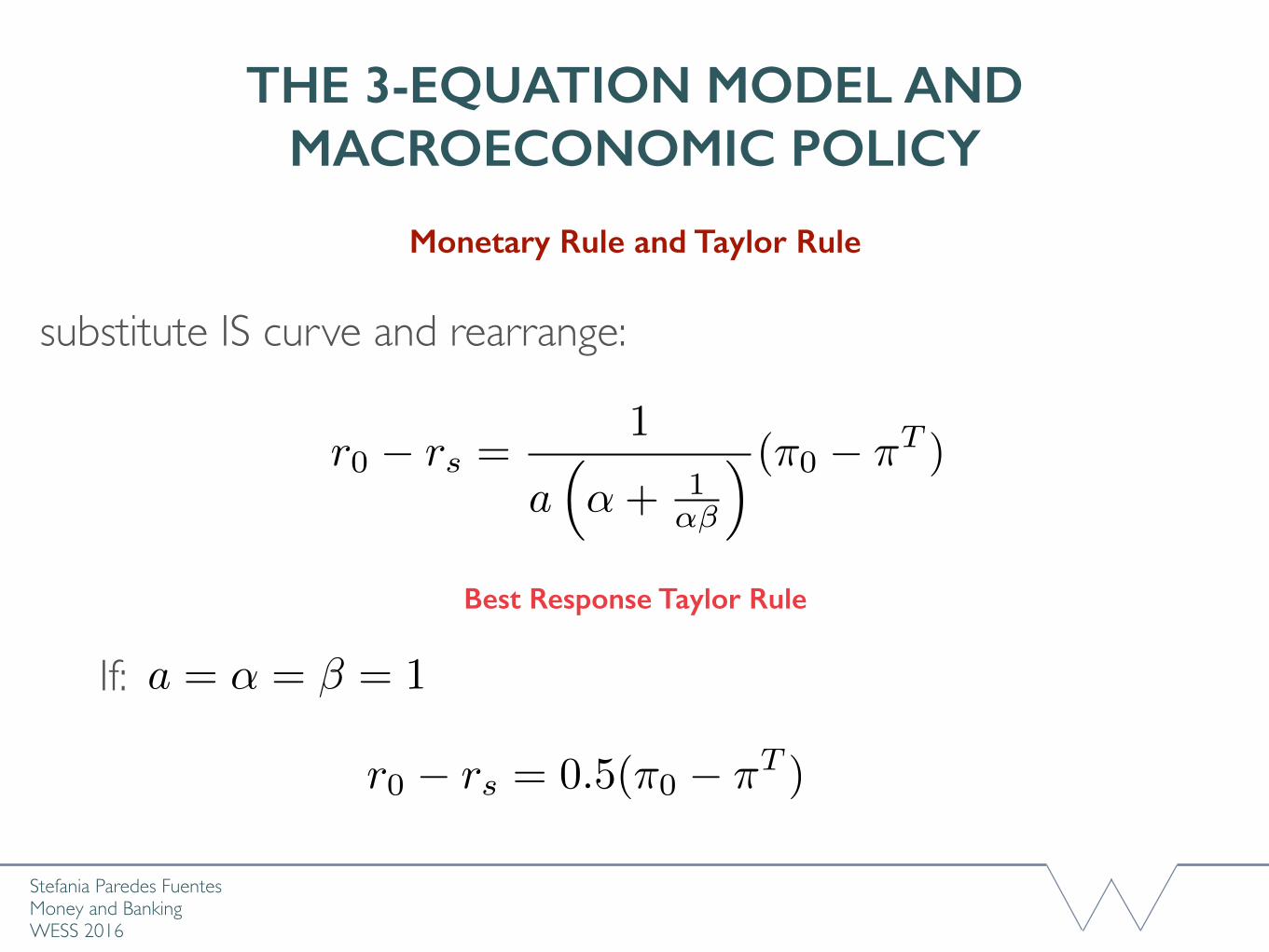
substitute IS curve and rearrange:
r0 � rs =1
a⇣↵+ 1
↵�
⌘ (⇡0 � ⇡T )
If: a = ↵ = � = 1
r0 � rs = 0.5(⇡0 � ⇡T )
Best Response Taylor Rule
Stefania Paredes Fuentes Money and BankingWESS 2016
THE 3-EQUATION MODEL AND MACROECONOMIC POLICY
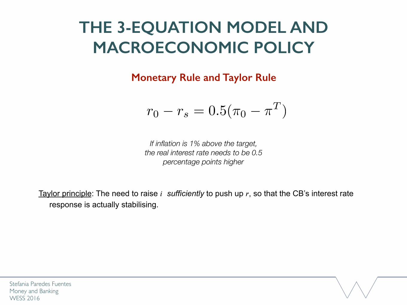
Monetary Rule and Taylor Rule
r0 � rs = 0.5(⇡0 � ⇡T )
If inflation is 1% above the target, the real interest rate needs to be 0.5
percentage points higher
Taylor principle: The need to raise 𝑖 sufficiently to push up 𝑟, so that the CB’s interest rate response is actually stabilising.
Stefania Paredes Fuentes Money and BankingWESS 2016
THE 3-EQUATION MODEL AND MACROECONOMIC POLICY
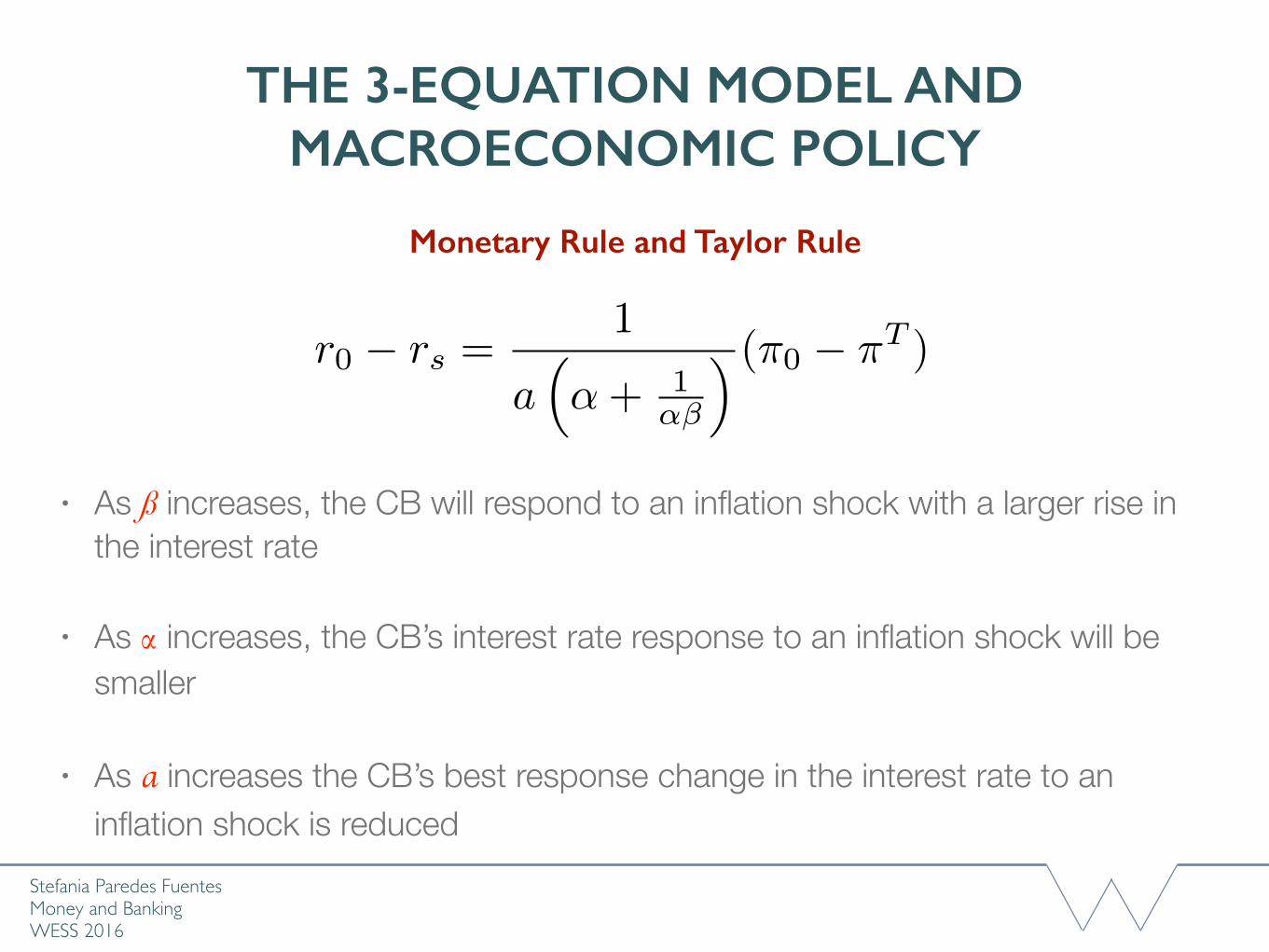
Monetary Rule and Taylor Rule
r0 � rs =1
a⇣↵+ 1
↵�
⌘ (⇡0 � ⇡T )
• As ß increases, the CB will respond to an inflation shock with a larger rise in the interest rate
• As α increases, the CB’s interest rate response to an inflation shock will be smaller
• As a increases the CB’s best response change in the interest rate to an inflation shock is reduced
Stefania Paredes Fuentes Money and BankingWESS 2016
THE 3-EQUATION MODEL AND MACROECONOMIC POLICY
Monetary Rule and Taylor Rule
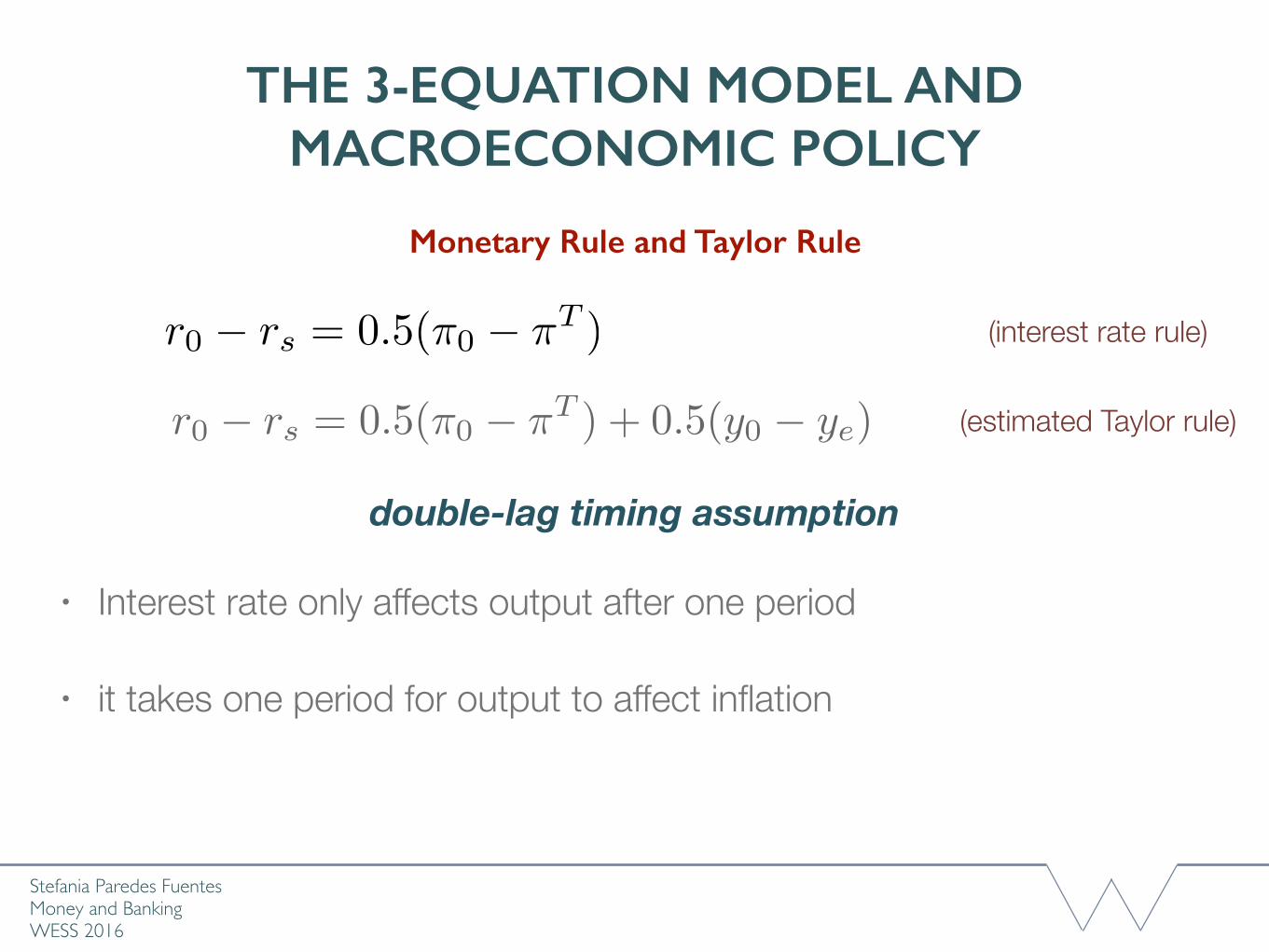
r0 � rs = 0.5(⇡0 � ⇡T )
• Interest rate only affects output after one period
• it takes one period for output to affect inflation
r0 � rs = 0.5(⇡0 � ⇡T ) + 0.5(y0 � ye) (estimated Taylor rule)
double-lag timing assumption
(interest rate rule)
Stefania Paredes Fuentes Money and BankingWESS 2016
THE 3-EQUATION MODEL AND MACROECONOMIC POLICY
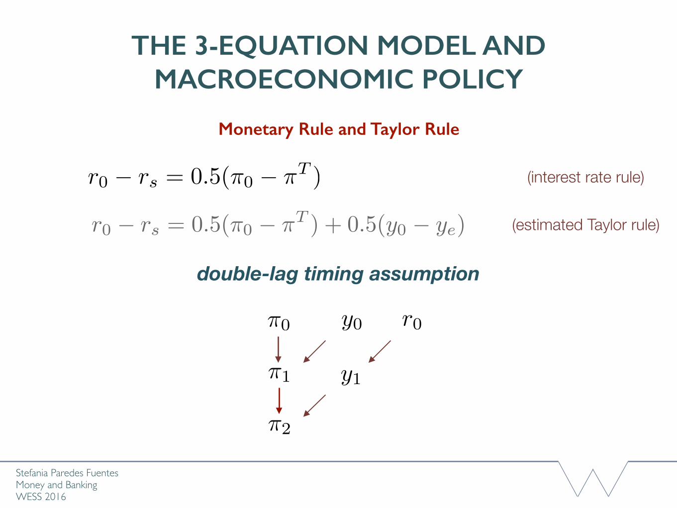
Monetary Rule and Taylor Rule
r0 � rs = 0.5(⇡0 � ⇡T )
r0 � rs = 0.5(⇡0 � ⇡T ) + 0.5(y0 � ye) (estimated Taylor rule)
double-lag timing assumption
(interest rate rule)
⇡0
⇡1
⇡2
y0
y1
r0
Stefania Paredes Fuentes Money and BankingWESS 2016
THE 3-EQUATION MODEL AND MACROECONOMIC POLICY
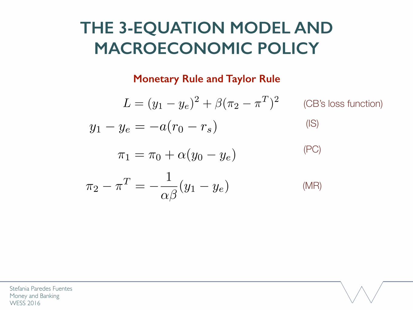
Monetary Rule and Taylor Rule
(CB’s loss function)
(PC)
L = (y1 � ye)2 + �(⇡2 � ⇡T )2
⇡1 = ⇡0 + ↵(y0 � ye)
y1 � ye = �a(r0 � rs) (IS)
⇡2 � ⇡T = � 1
↵�(y1 � ye) (MR)
Stefania Paredes Fuentes Money and BankingWESS 2016
THE 3-EQUATION MODEL AND MACROECONOMIC POLICY
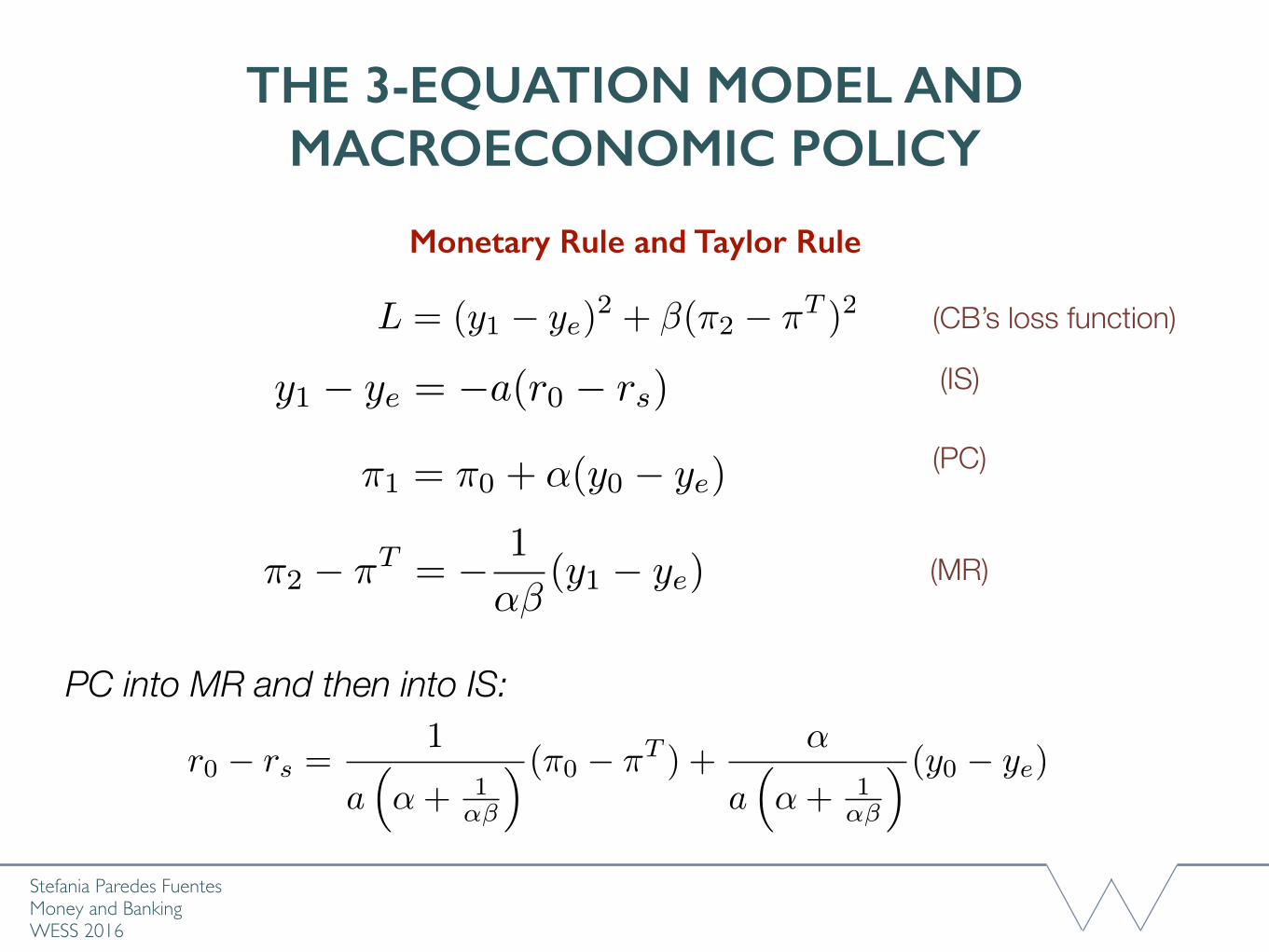
Monetary Rule and Taylor Rule
(CB’s loss function)
(PC)
L = (y1 � ye)2 + �(⇡2 � ⇡T )2
⇡1 = ⇡0 + ↵(y0 � ye)
y1 � ye = �a(r0 � rs) (IS)
⇡2 � ⇡T = � 1
↵�(y1 � ye) (MR)
PC into MR and then into IS:
r0 � rs =1
a⇣↵+ 1
↵�
⌘ (⇡0 � ⇡T ) +↵
a⇣↵+ 1
↵�
⌘ (y0 � ye)
Stefania Paredes Fuentes Money and BankingWESS 2016
THE 3-EQUATION MODEL AND MACROECONOMIC POLICY
Monetary Rule and Taylor Rule
r0 � rs =1
a⇣↵+ 1
↵�
⌘ (⇡0 � ⇡T ) +↵
a⇣↵+ 1
↵�
⌘ (y0 � ye)
a = ↵ = � = 1
r0 � rs = 0.5(⇡0 � ⇡T ) + 0.5(y0 � ye)
(estimated Taylor rule)
Stefania Paredes Fuentes Money and BankingWESS 2016
THE 3-EQUATION MODEL AND MACROECONOMIC POLICY
Monetary Rule and Taylor Rule

3 EQUATION MODEL AND THE BANKING SYSTEM
Stefania Paredes Fuentes Money and BankingWESS 2016
y
π
ye
πT = πE
PC(πtE = πT)
A
y
rs
IS
A
r
MR
�1
a
� 1
↵�
↵
yt = At � art�1
⇡t = ⇡t�1 + ↵(y � ye)
(yt � ye) = �↵�(⇡t � ⇡T )
Stefania Paredes Fuentes Money and BankingWESS 2016
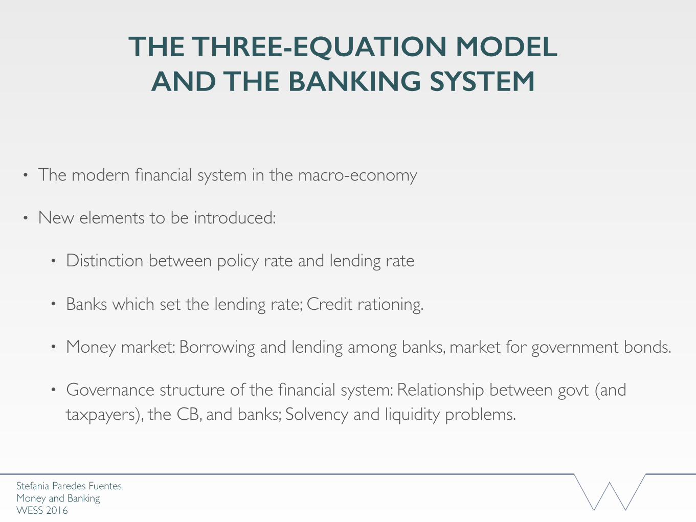
THE THREE-EQUATION MODEL AND THE BANKING SYSTEM
• The modern financial system in the macro-economy
• New elements to be introduced:
• Distinction between policy rate and lending rate
• Banks which set the lending rate; Credit rationing.
• Money market: Borrowing and lending among banks, market for government bonds.
• Governance structure of the financial system: Relationship between govt (and taxpayers), the CB, and banks; Solvency and liquidity problems.
Stefania Paredes Fuentes Money and BankingWESS 2016
THE THREE-EQUATION MODEL AND THE BANKING SYSTEM
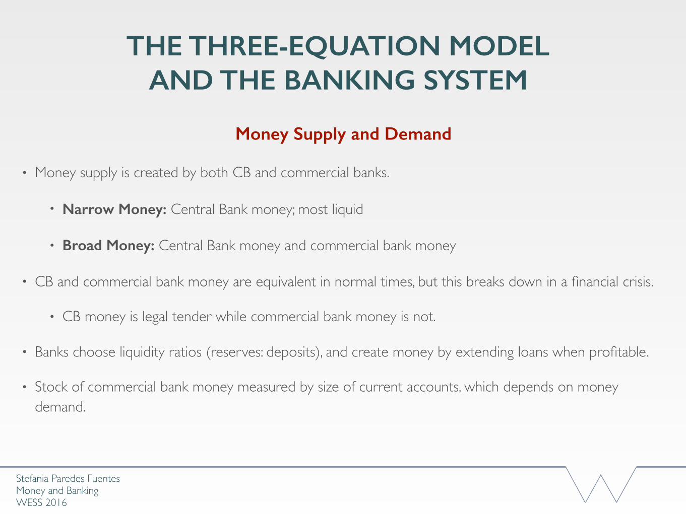
• Money supply is created by both CB and commercial banks.
• Narrow Money: Central Bank money; most liquid
• Broad Money: Central Bank money and commercial bank money
• CB and commercial bank money are equivalent in normal times, but this breaks down in a financial crisis.
• CB money is legal tender while commercial bank money is not.
• Banks choose liquidity ratios (reserves: deposits), and create money by extending loans when profitable.
• Stock of commercial bank money measured by size of current accounts, which depends on money demand.
Money Supply and Demand
Stefania Paredes Fuentes Money and BankingWESS 2016
THE THREE-EQUATION MODEL AND THE BANKING SYSTEM
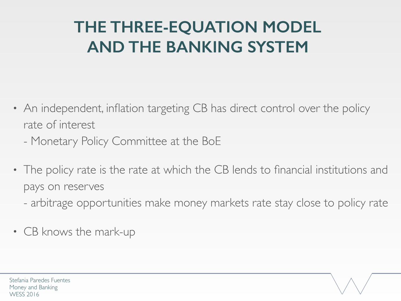
• An independent, inflation targeting CB has direct control over the policy rate of interest - Monetary Policy Committee at the BoE
• The policy rate is the rate at which the CB lends to financial institutions and pays on reserves - arbitrage opportunities make money markets rate stay close to policy rate
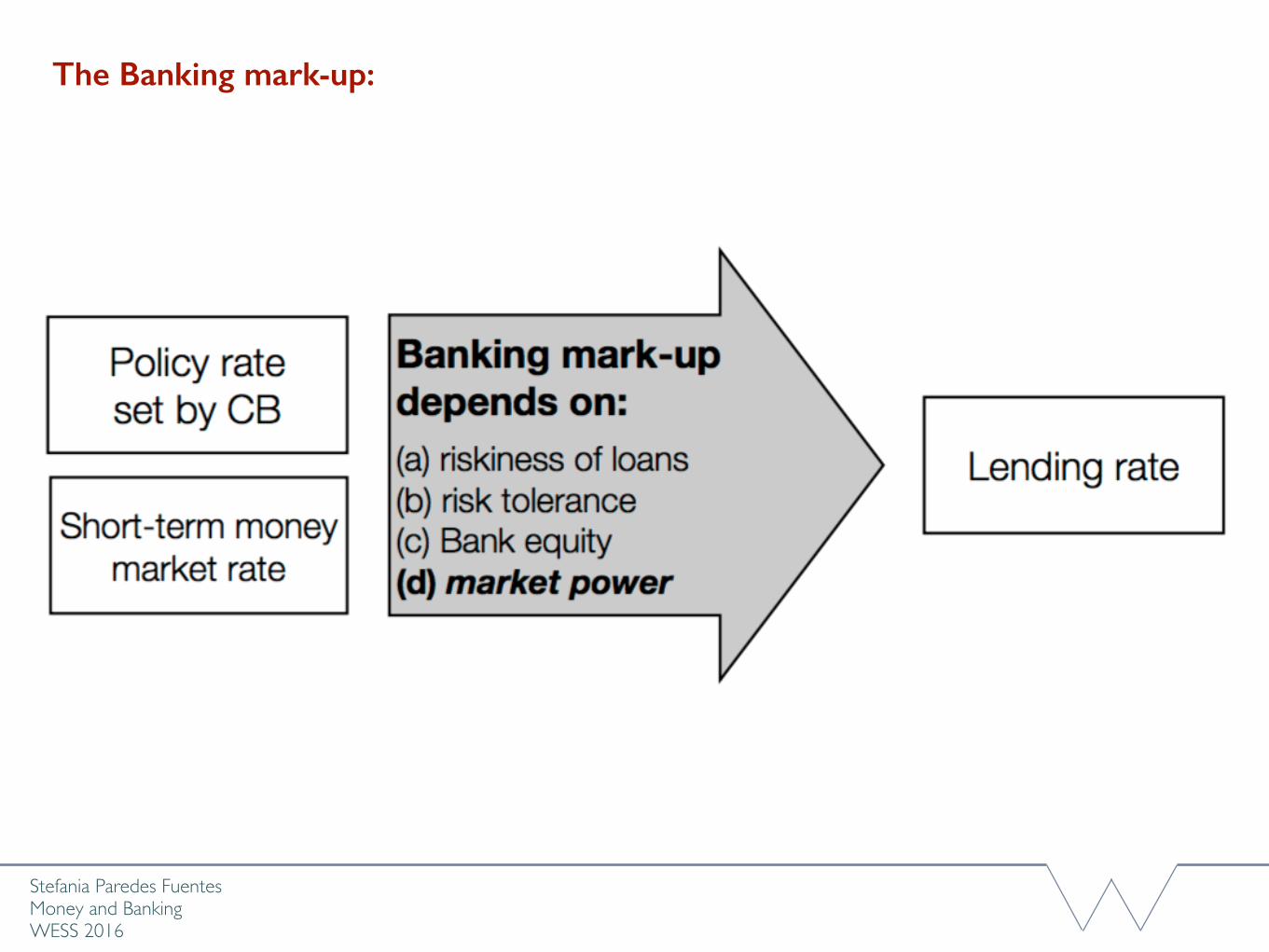
• CB knows the mark-up
Stefania Paredes Fuentes Money and BankingWESS 2016
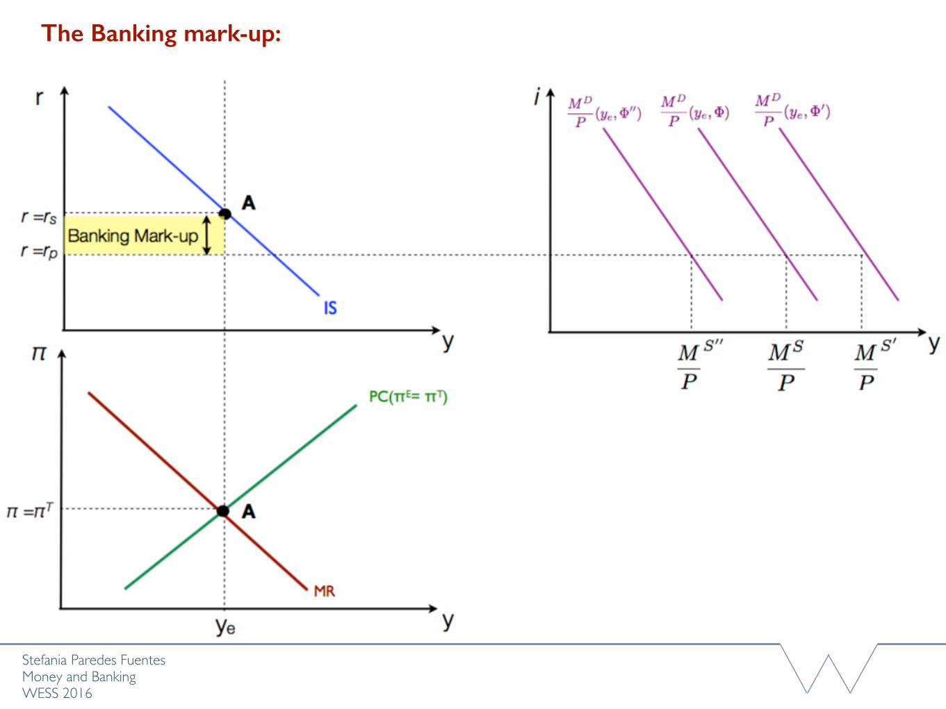
The Banking mark-up:
Stefania Paredes Fuentes Money and BankingWESS 2016
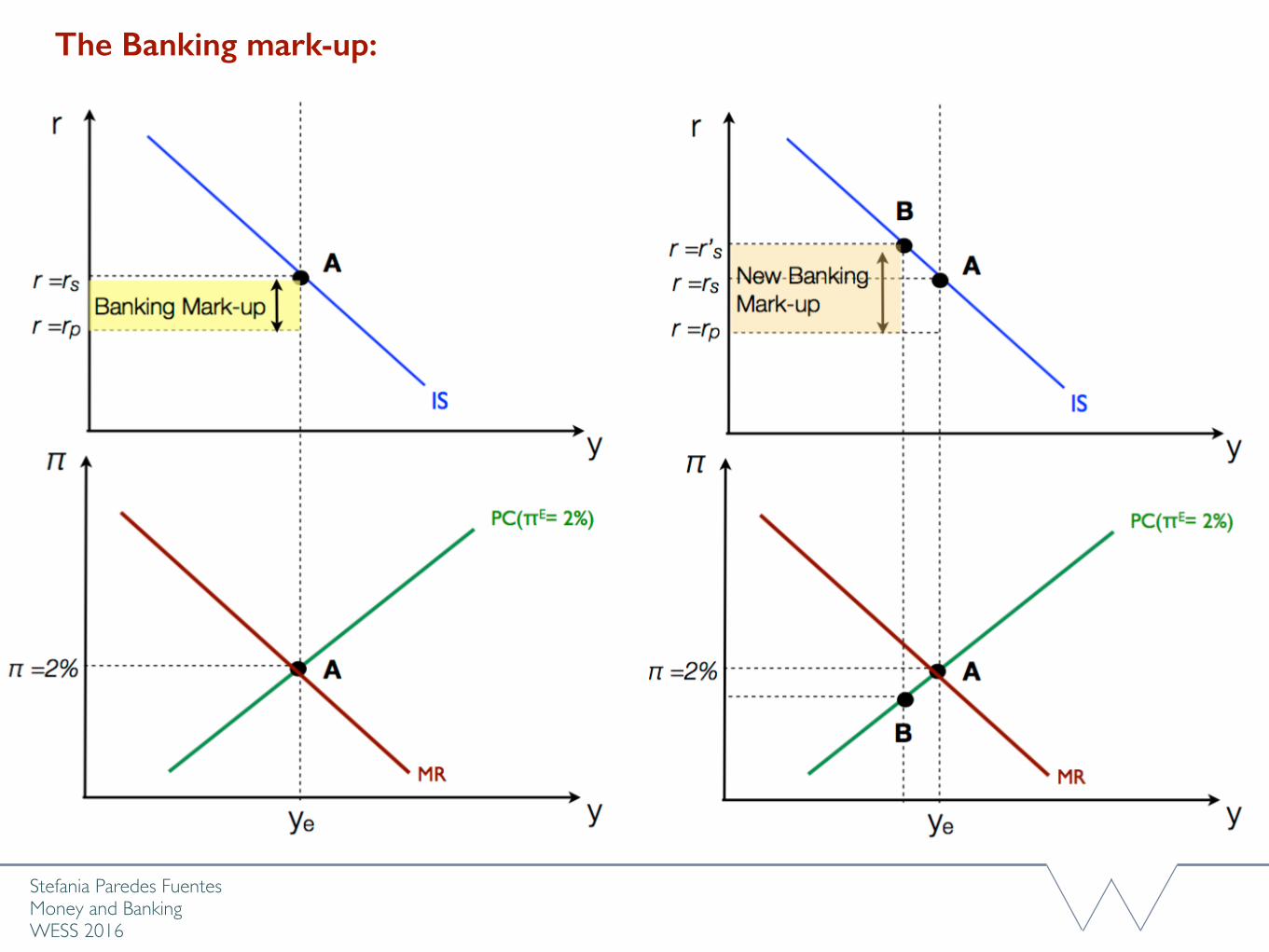
The Banking mark-up:
Stefania Paredes Fuentes Money and BankingWESS 2016
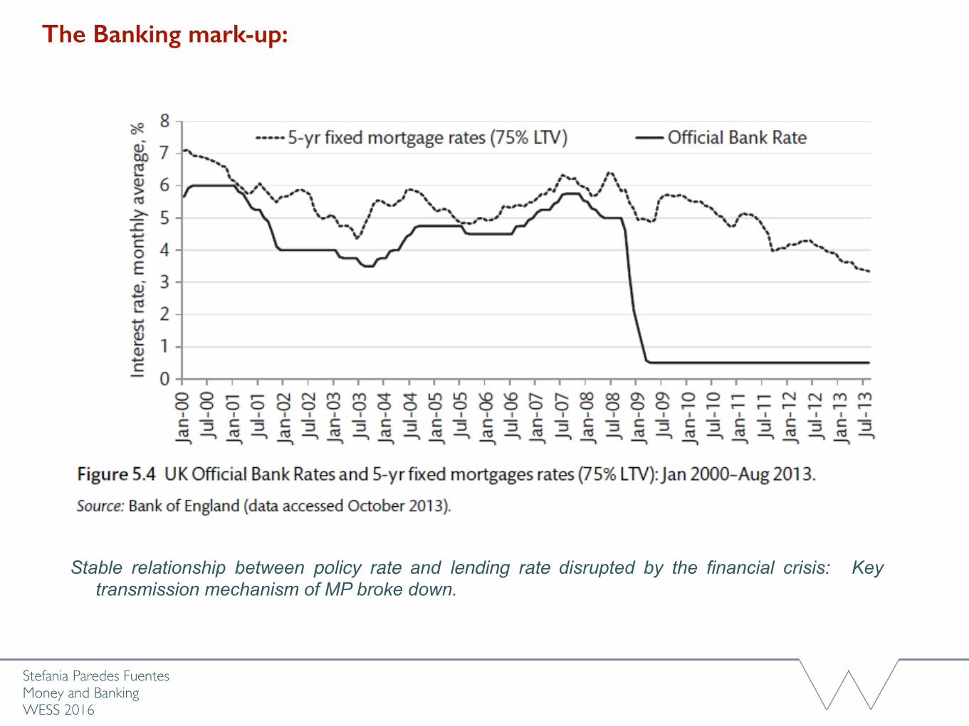
The Banking mark-up:
Stable relationship between policy rate and lending rate disrupted by the financial crisis: Key transmission mechanism of MP broke down.
Stefania Paredes Fuentes Money and BankingWESS 2016
THE THREE-EQUATION MODEL AND THE BANKING SYSTEM
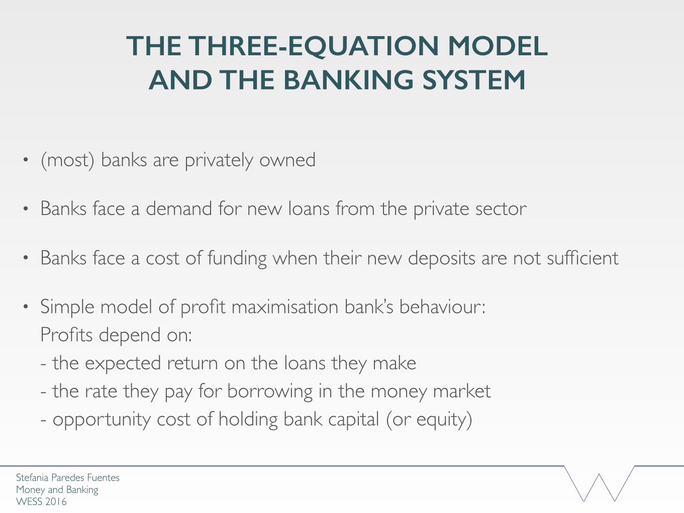
• (most) banks are privately owned
• Banks face a demand for new loans from the private sector
• Banks face a cost of funding when their new deposits are not sufficient
• Simple model of profit maximisation bank’s behaviour:Profits depend on:- the expected return on the loans they make - the rate they pay for borrowing in the money market- opportunity cost of holding bank capital (or equity)
Stefania Paredes Fuentes Money and BankingWESS 2016
The Banking mark-up:
Stefania Paredes Fuentes Money and BankingWESS 2016
THE THREE-EQUATION MODEL AND THE BANKING SYSTEM
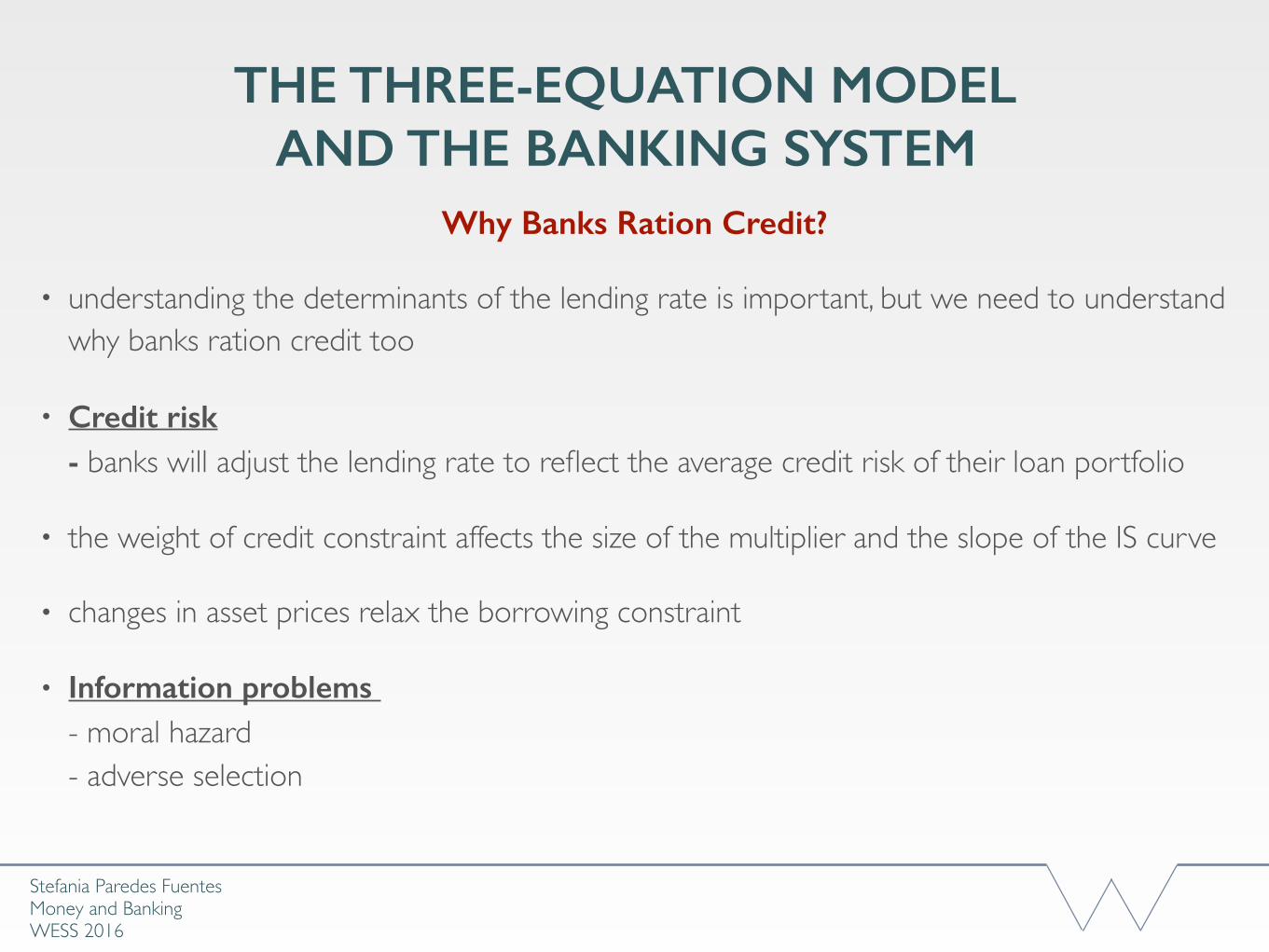
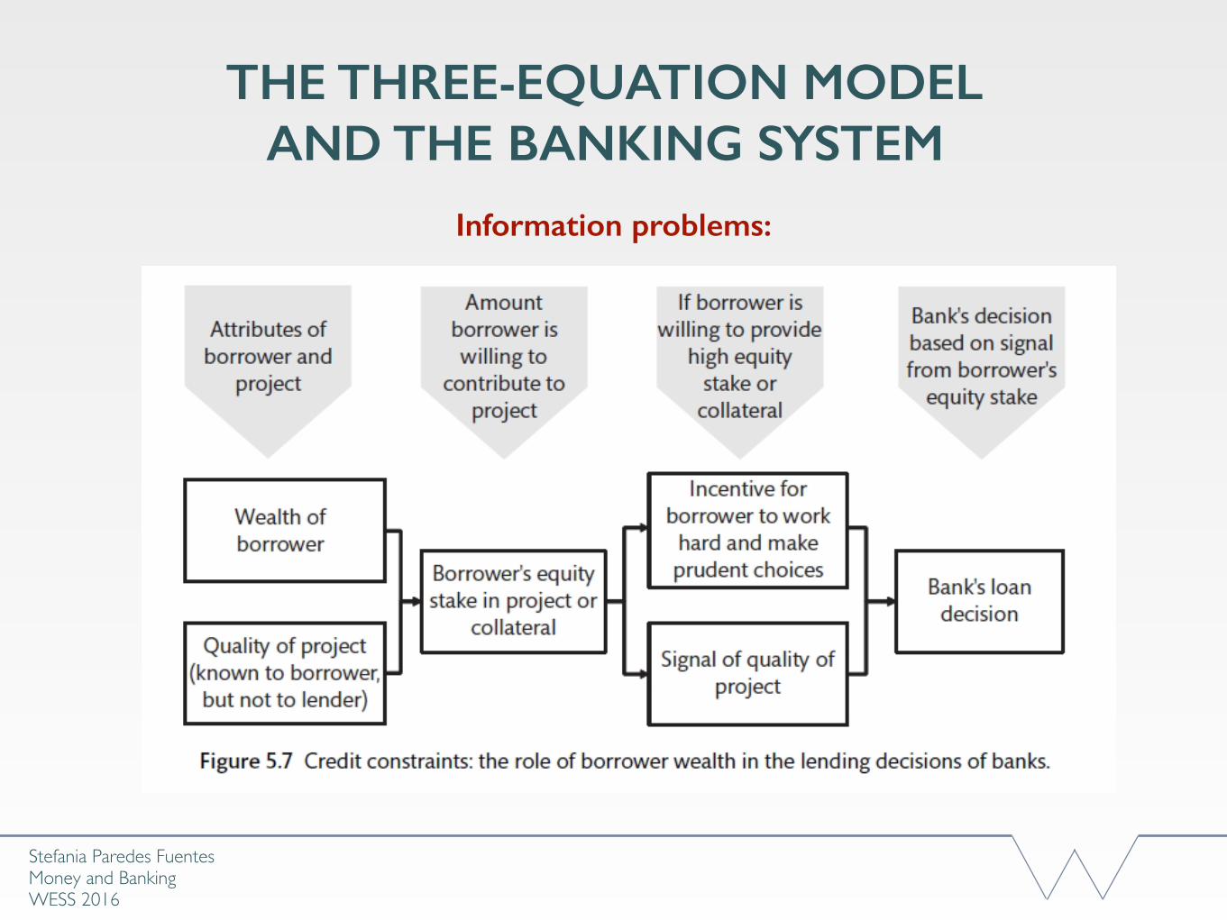
• understanding the determinants of the lending rate is important, but we need to understand why banks ration credit too
• Credit risk - banks will adjust the lending rate to reflect the average credit risk of their loan portfolio
• the weight of credit constraint affects the size of the multiplier and the slope of the IS curve
• changes in asset prices relax the borrowing constraint
• Information problems - moral hazard- adverse selection
Why Banks Ration Credit?
Stefania Paredes Fuentes Money and BankingWESS 2016
THE THREE-EQUATION MODEL AND THE BANKING SYSTEM
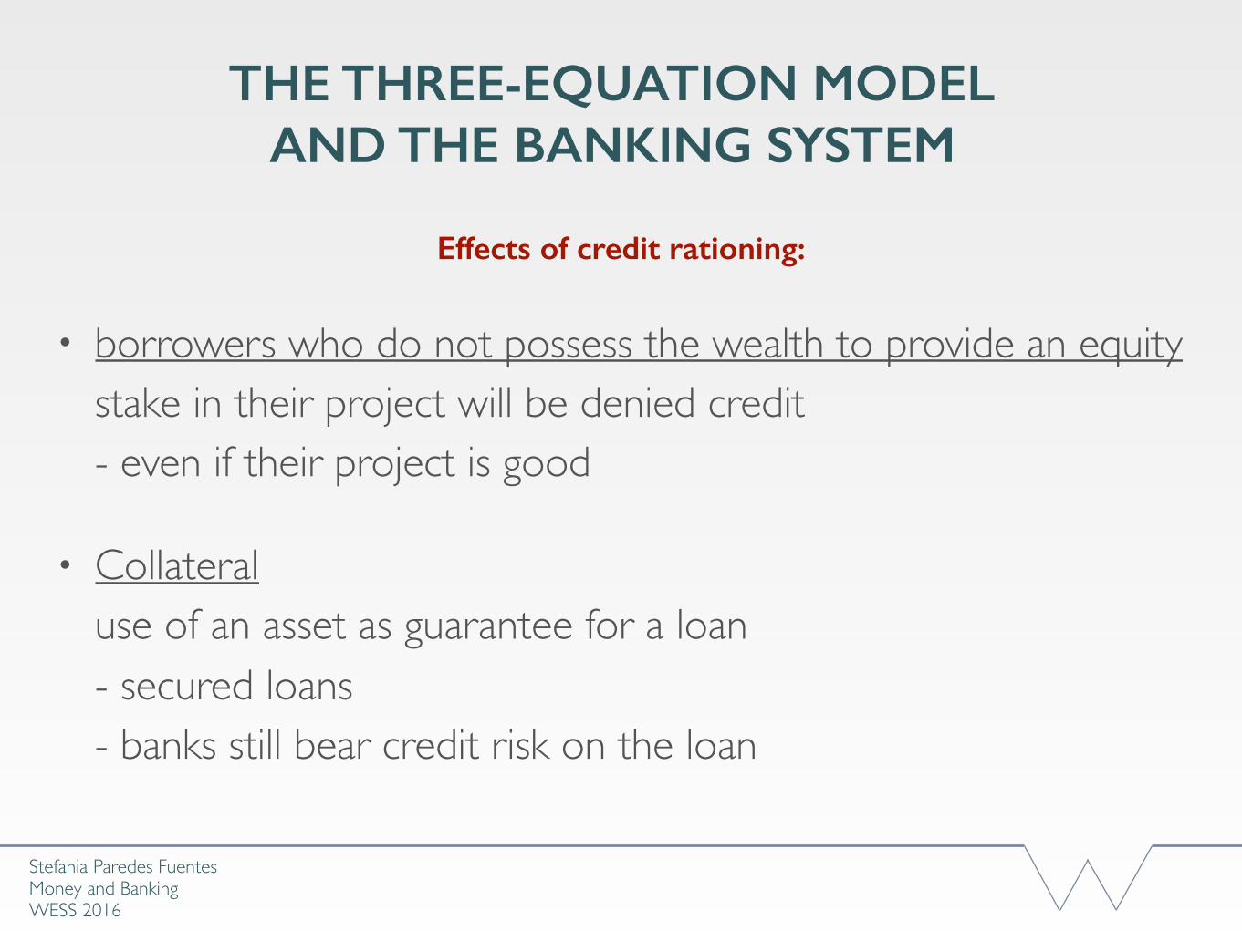
• borrowers who do not possess the wealth to provide an equity stake in their project will be denied credit- even if their project is good
• Collateraluse of an asset as guarantee for a loan - secured loans - banks still bear credit risk on the loan
Effects of credit rationing:
Stefania Paredes Fuentes Money and BankingWESS 2016
THE THREE-EQUATION MODEL AND THE BANKING SYSTEM
Information problems:
Stefania Paredes Fuentes Money and BankingWESS 2016
THE THREE-EQUATION MODEL AND THE BANKING SYSTEM
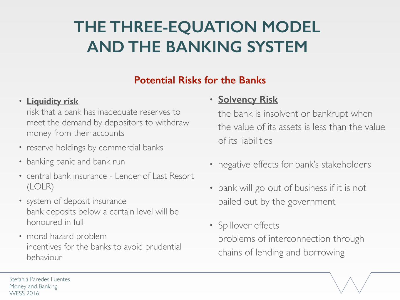
• Liquidity risk risk that a bank has inadequate reserves to meet the demand by depositors to withdraw money from their accounts
• reserve holdings by commercial banks• banking panic and bank run• central bank insurance - Lender of Last Resort
(LOLR)• system of deposit insurance
bank deposits below a certain level will be honoured in full
• moral hazard problemincentives for the banks to avoid prudential behaviour
Potential Risks for the Banks
• Solvency Risk the bank is insolvent or bankrupt when the value of its assets is less than the value of its liabilities
• negative effects for bank’s stakeholders
• bank will go out of business if it is not bailed out by the government
• Spillover effectsproblems of interconnection through chains of lending and borrowing
Stefania Paredes Fuentes Money and BankingWESS 2016
THE THREE-EQUATION MODEL AND THE BANKING SYSTEM
• Schemes to prevent liquidity problems (LOLR facility and deposit guarantees) have to be designed to tread the fine line between:
• Protecting the public from the spillovers of liquidity problems• Avoiding moral hazard• Such schemes make banks less prudent in their lending behaviour, and households less
prudent in their savings behaviour (Households might save in unsound banks, since their deposits are guaranteed anyway)
• Solvency risk: when the value of assets is less than that of debts or liabilities → bankruptcy if not bailed out by the government.
• Interconnectedness in the banking sector: Solvency problem for a small no. of banks → banks unsure about safety in borrowing from one another → widespread liquidity problems
• Insolvency has direct negative effects on bank depositors, creditors, shareholders and bondholders.
How to prevent liquidity problems
Stefania Paredes Fuentes Money and BankingWESS 2016
THE THREE-EQUATION MODEL AND THE BANKING SYSTEM
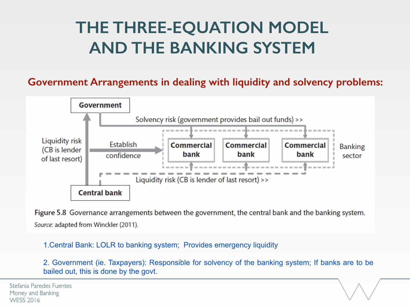
Government Arrangements in dealing with liquidity and solvency problems:
1.Central Bank: LOLR to banking system; Provides emergency liquidity
2. Government (ie. Taxpayers): Responsible for solvency of the banking system; If banks are to be bailed out, this is done by the govt.
Stefania Paredes Fuentes Money and BankingWESS 2016
THE THREE-EQUATION MODEL AND THE BANKING SYSTEM
Government Arrangements in dealing with liquidity and solvency problems:
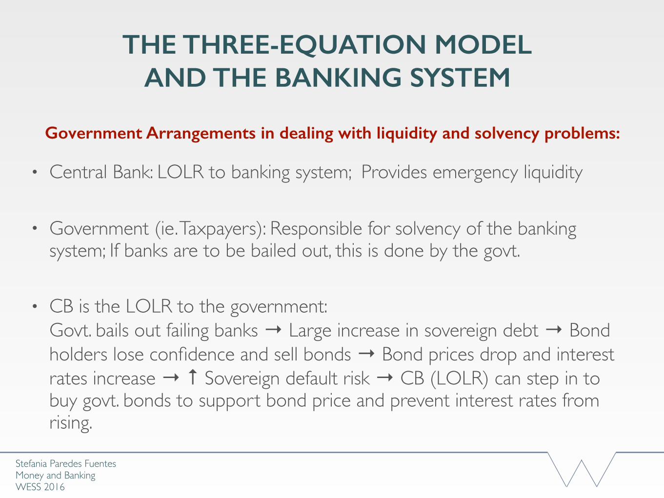
• Central Bank: LOLR to banking system; Provides emergency liquidity
• Government (ie. Taxpayers): Responsible for solvency of the banking system; If banks are to be bailed out, this is done by the govt.
• CB is the LOLR to the government:Govt. bails out failing banks → Large increase in sovereign debt → Bond holders lose confidence and sell bonds → Bond prices drop and interest rates increase → ↑ Sovereign default risk → CB (LOLR) can step in to buy govt. bonds to support bond price and prevent interest rates from rising.
Stefania Paredes Fuentes Money and BankingWESS 2016
THE THREE-EQUATION MODEL AND THE BANKING SYSTEM
Government Arrangements in dealing with liquidity and solvency problems:
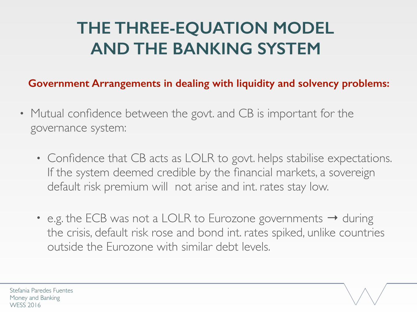
• Mutual confidence between the govt. and CB is important for the governance system:
• Confidence that CB acts as LOLR to govt. helps stabilise expectations. If the system deemed credible by the financial markets, a sovereign default risk premium will not arise and int. rates stay low.
• e.g. the ECB was not a LOLR to Eurozone governments → during the crisis, default risk rose and bond int. rates spiked, unlike countries outside the Eurozone with similar debt levels.
Stefania Paredes Fuentes Money and BankingWESS 2016
THE THREE-EQUATION MODEL AND THE BANKING SYSTEM
Eurozone:
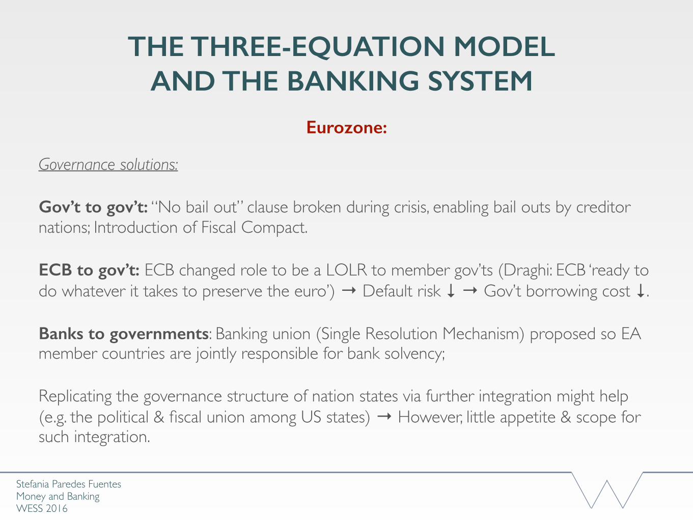
Governance solutions:
Gov’t to gov’t: “No bail out” clause broken during crisis, enabling bail outs by creditor nations; Introduction of Fiscal Compact.
ECB to gov’t: ECB changed role to be a LOLR to member gov’ts (Draghi: ECB ‘ready to do whatever it takes to preserve the euro’) → Default risk ↓ → Gov’t borrowing cost ↓.
Banks to governments: Banking union (Single Resolution Mechanism) proposed so EA member countries are jointly responsible for bank solvency;
Replicating the governance structure of nation states via further integration might help (e.g. the political & fiscal union among US states) → However, little appetite & scope for such integration.
Stefania Paredes Fuentes Money and BankingWESS 2016
THE THREE-EQUATION MODEL AND THE BANKING SYSTEM
Eurozone:
Perhaps they will be lucky. It may be that events, as they turn out in the next 10 or 20 years, will be common to all the countries; there will be no shocks, no economic developments that affect the different parts of the Euro area asymmetrically. In that case, they'll get along fine and perhaps the separate countries will gradually loosen up their arrangements, get rid of some of their restrictions and open up so that they're more adaptable, more flexible.
On the other hand, the more likely possibility is that there will be asymmetric shocks hitting the different countries. That will mean that the only adjustment mechanism they have to meet that with is fiscal and unemployment: pressure on wages, pressure on prices. They have no way out.
Milton Friedman, 1998
Stefania Paredes Fuentes Money and BankingWESS 2016
THE THREE-EQUATION MODEL AND THE BANKING SYSTEM
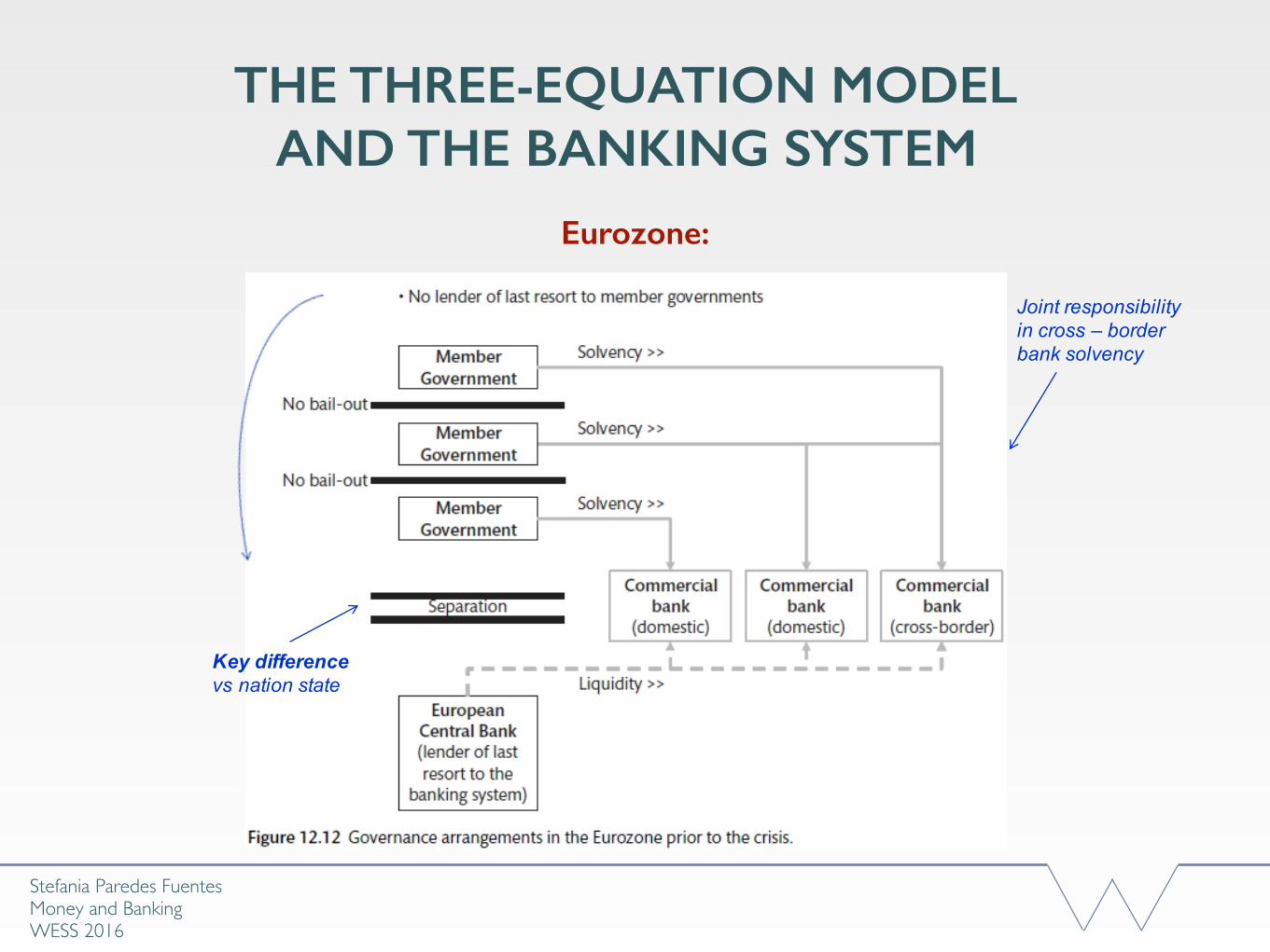
Eurozone:
Key differencevs nation state
Joint responsibility in cross – border bank solvency
Stefania Paredes Fuentes Money and BankingWESS 2016
THE THREE-EQUATION MODEL AND THE BANKING SYSTEM
Eurozone:
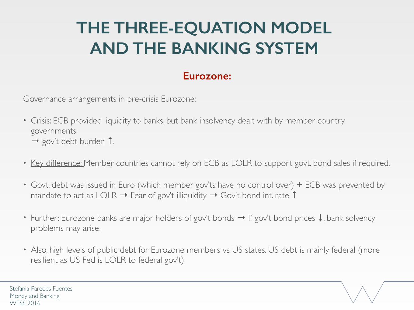
Governance arrangements in pre-crisis Eurozone:
• Crisis: ECB provided liquidity to banks, but bank insolvency dealt with by member country governments → gov’t debt burden ↑.
• Key difference: Member countries cannot rely on ECB as LOLR to support govt. bond sales if required.
• Govt. debt was issued in Euro (which member gov’ts have no control over) + ECB was prevented by mandate to act as LOLR → Fear of gov’t illiquidity → Gov’t bond int. rate ↑
• Further: Eurozone banks are major holders of gov’t bonds → If gov’t bond prices ↓, bank solvency problems may arise.
• Also, high levels of public debt for Eurozone members vs US states. US debt is mainly federal (more resilient as US Fed is LOLR to federal gov’t)
Stefania Paredes Fuentes Money and BankingWESS 2016
THE THREE-EQUATION MODEL AND THE BANKING SYSTEM
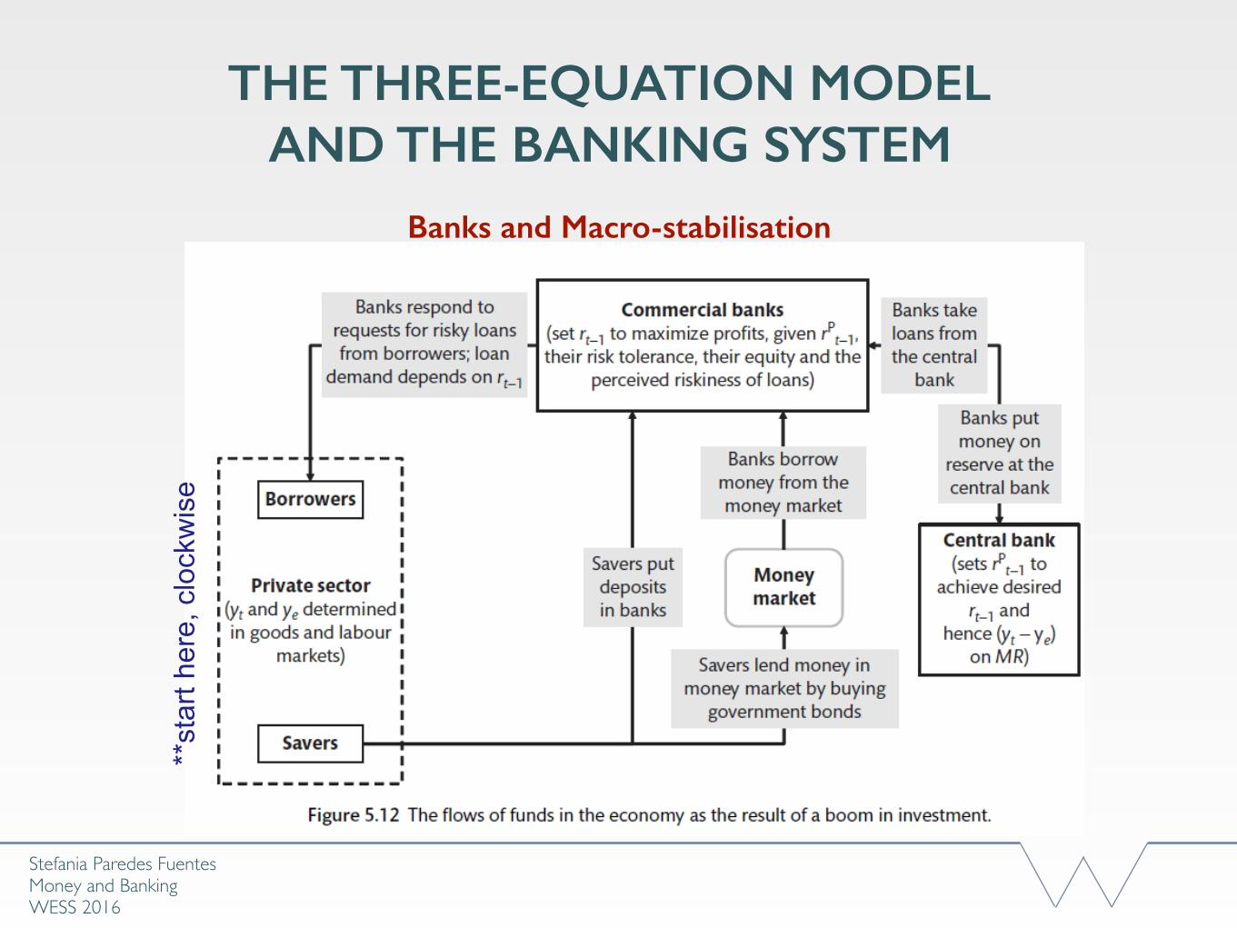
Banks and Macro-stabilisation
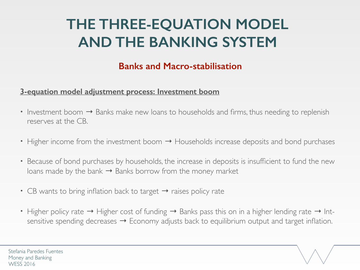
3-equation model adjustment process: Investment boom
• Investment boom → Banks make new loans to households and firms, thus needing to replenish reserves at the CB.
• Higher income from the investment boom → Households increase deposits and bond purchases
• Because of bond purchases by households, the increase in deposits is insufficient to fund the new loans made by the bank → Banks borrow from the money market
• CB wants to bring inflation back to target → raises policy rate
• Higher policy rate → Higher cost of funding → Banks pass this on in a higher lending rate → Int-sensitive spending decreases → Economy adjusts back to equilibrium output and target inflation.
Stefania Paredes Fuentes Money and BankingWESS 2016
THE THREE-EQUATION MODEL AND THE BANKING SYSTEM
Banks and Macro-stabilisation**
star
t her
e, c
lock
wis
e
Stefania Paredes Fuentes Money and BankingWESS 2016
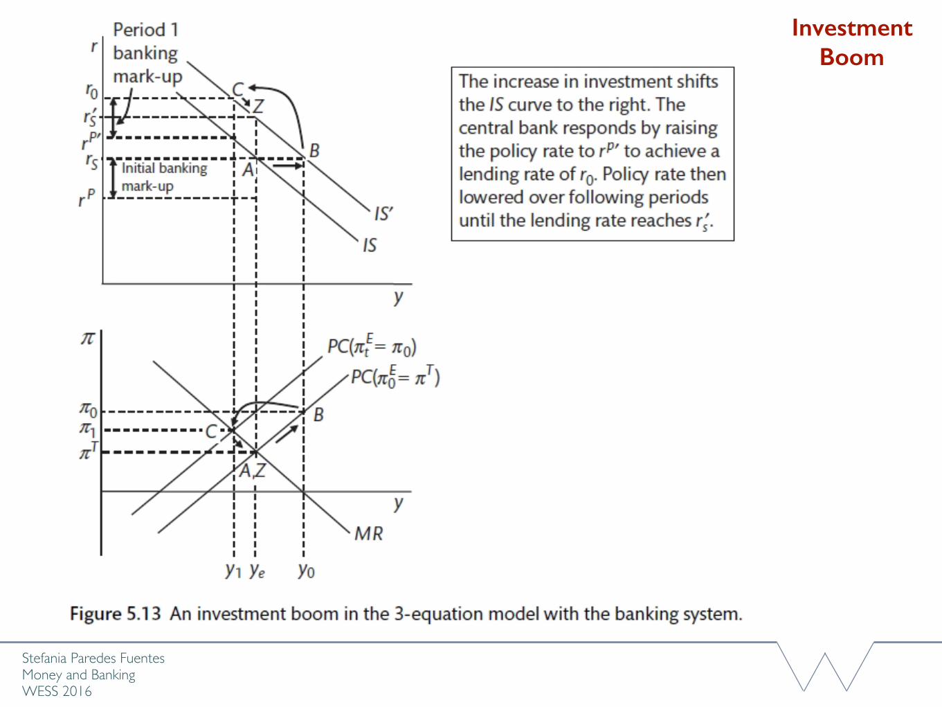
Investment Boom
Stefania Paredes Fuentes Money and BankingWESS 2016
THE THREE-EQUATION MODEL AND THE BANKING SYSTEM
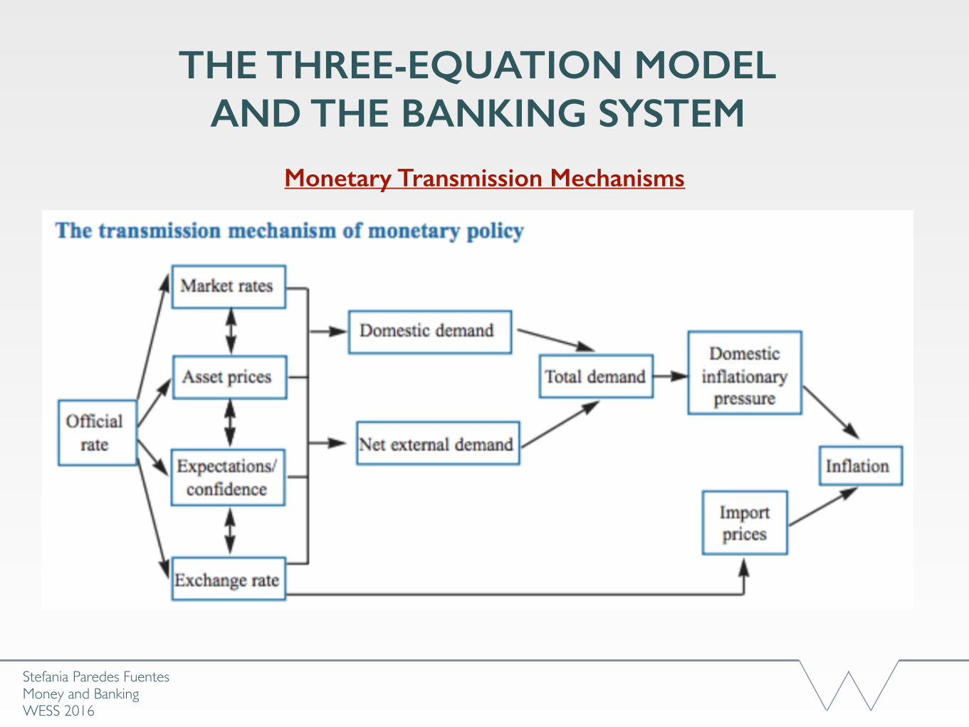
Monetary Transmission Mechanisms
Stefania Paredes Fuentes Money and BankingWESS 2016
THE THREE-EQUATION MODEL AND THE BANKING SYSTEM
Monetary Transmission Mechanisms
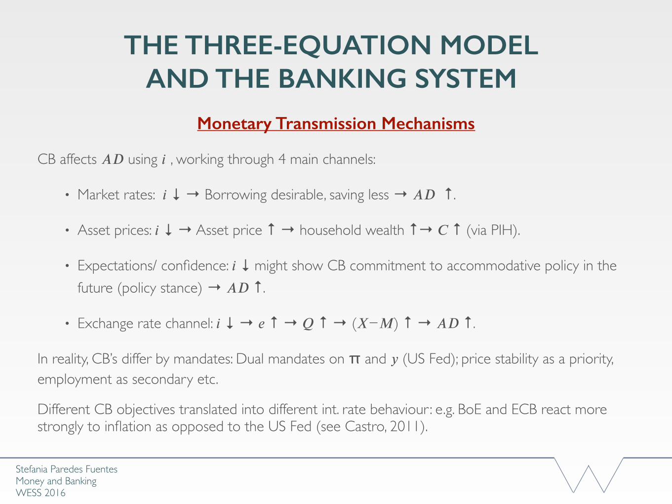
CB affects 𝐴𝐷 using 𝑖 , working through 4 main channels:
• Market rates: 𝑖 ↓ → Borrowing desirable, saving less → 𝐴𝐷 ↑.
• Asset prices: 𝑖 ↓ → Asset price ↑ → household wealth ↑→ 𝐶 ↑ (via PIH).
• Expectations/ confidence: 𝑖 ↓ might show CB commitment to accommodative policy in the future (policy stance) → 𝐴𝐷 ↑.
• Exchange rate channel: 𝑖 ↓ → 𝑒 ↑ → 𝑄 ↑ → (𝑋−𝑀) ↑ → 𝐴𝐷 ↑.
In reality, CB’s differ by mandates: Dual mandates on π and 𝑦 (US Fed); price stability as a priority, employment as secondary etc.
Different CB objectives translated into different int. rate behaviour: e.g. BoE and ECB react more strongly to inflation as opposed to the US Fed (see Castro, 2011).
THE 3-EQUATION MODEL AND MACROECONOMIC POLICY
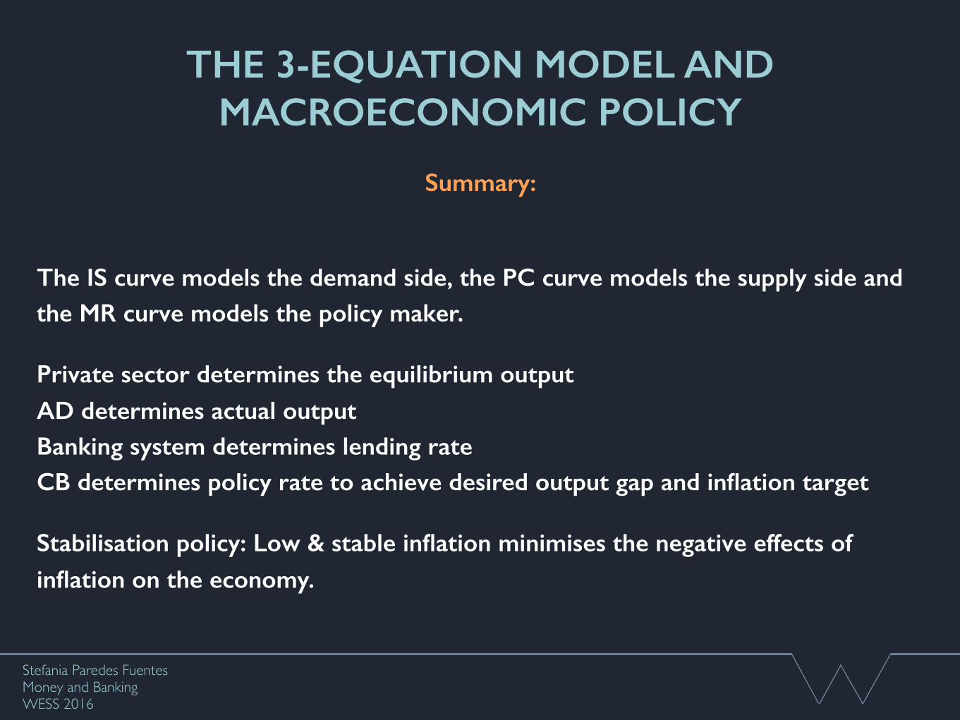
The IS curve models the demand side, the PC curve models the supply side and the MR curve models the policy maker.
Private sector determines the equilibrium output AD determines actual output Banking system determines lending rate CB determines policy rate to achieve desired output gap and inflation target
Stabilisation policy: Low & stable inflation minimises the negative effects of inflation on the economy.
Stefania Paredes Fuentes Money and BankingWESS 2016
Summary:
THE 3-EQUATION MODEL AND MACROECONOMIC POLICY
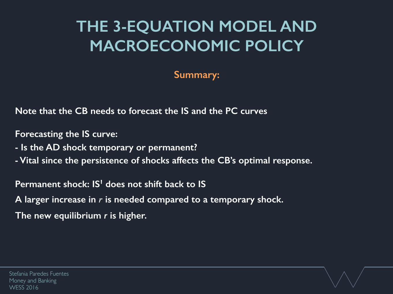
Note that the CB needs to forecast the IS and the PC curves
Forecasting the IS curve: - Is the AD shock temporary or permanent? - Vital since the persistence of shocks affects the CB’s optimal response.
Permanent shock: ISꞌ does not shift back to IS A larger increase in 𝑟 is needed compared to a temporary shock. The new equilibrium r is higher.
Stefania Paredes Fuentes Money and BankingWESS 2016
Summary:
THE 3-EQUATION MODEL AND MACROECONOMIC POLICY
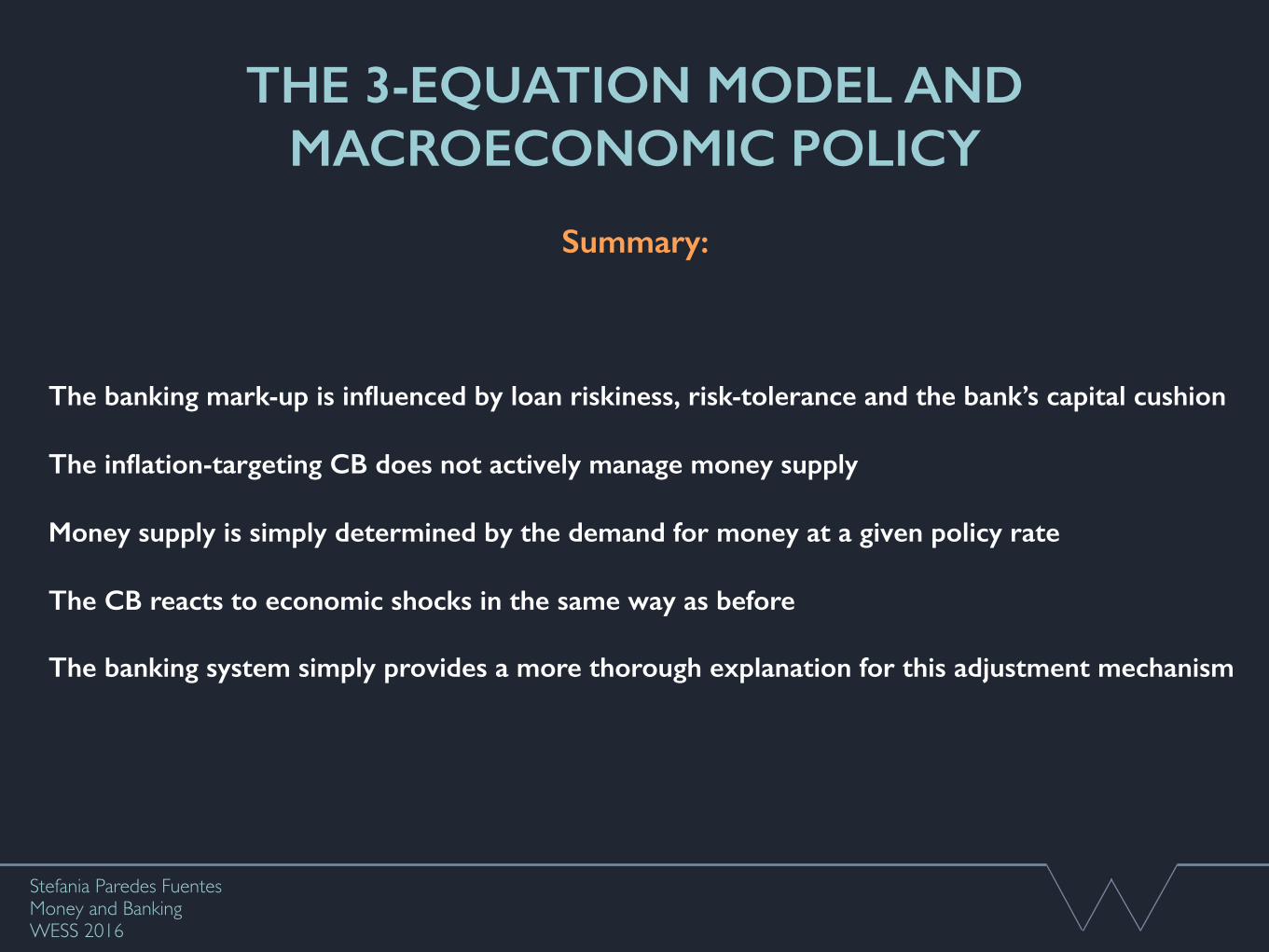
The banking mark-up is influenced by loan riskiness, risk-tolerance and the bank’s capital cushion
The inflation-targeting CB does not actively manage money supply
Money supply is simply determined by the demand for money at a given policy rate
The CB reacts to economic shocks in the same way as before
The banking system simply provides a more thorough explanation for this adjustment mechanism
Stefania Paredes Fuentes Money and BankingWESS 2016
Summary:
SOME READINGS• Carlin & Soskice, Chapters 3, 5 & 13 (1 & 2 if you need to refresh basic macro)
• Carvalho, A. & C. Gonçalves (2009). Inflation Targeting Matters: Evidence from OECD Economies’s Sacrifice Ratios. Journal of Money, Credit and Banking 41(1)
• Romer D. (2000). Keynesian Macroeconomics Without the LM Curve. Journal of Economic Perspectives, Vol. 14(2), pp. 149-69
• Taylor, J. (1993). Discretion vs Policy Rules in Practice. Carnegie-Rochester Confer- ence Series on Public Policy 39, pp. 195-214.
• Castro, V. (2011). Can Central Banks’s Monetary Policy be described by a linear (augmented) Taylor Rule or by A Non-Linear Rule? Journal of Financial Stability, 7(4)
• King, M. (1997) The Inflation Target Five Years On. Available at: http://www.bankofengland.co.uk/archive/Documents/historicpubs/speeches/1997/sp eech09.pdf
• King, M. (2012) Twenty Year of Inflation Targeting. Available at: http://www.bankofengland.co.uk/publications/Documents/speeches/2012/speech606. pdf
• Fischer, Stanley, 1990. "Rules versus discretion in monetary policy," Handbook of Monetary Economics, in: B. M. Friedman & F. H. Hahn (ed.), Handbook of Monetary Economics, edition 1, volume 2, chapter 21, pages 1155-1184 Elsevier.Available at: http://www.nber.org/papers/w2518
• Nikolsko‐Rzhevskyy, Alex and Papell, David H. and Prodan, Ruxandra, (Taylor) Rules versus Discretion in U.S. Monetary Policy (August 2, 2013). Available at SSRN: http://ssrn.com/abstract=2294990
• Goodfriend, Marvin. 2007. “How the World Achieved Consensus on Monetary Policy.” Journal of Economic Perspectives 21 (4):47-68.
• Schiller, R J (1997) ‘Why Do People Dislike Inflation’ in Reducing Inflation: Motivation and Strategy, ads Christina D. Romer and David H. Romer. University of Chicago Press
• Bank of England (2015). The Bank of England’s Sterling Monetary Framework. (“The Red Book”)
• The transmission mechanisms of monetary policy. Bank of England (last accessed 6th November 2015)