Solar PhysDOI 10.1007/s11207-013-0341-5

The 22-Year Hale Cycle in Cosmic Ray Flux – Evidencefor Direct Heliospheric Modulation

S.R. Thomas · M.J. Owens · M. Lockwood

Received: 21 May 2012 / Accepted: 29 May 2013© Springer Science+Business Media Dordrecht 2013

Abstract The ability to predict times of greater galactic cosmic ray (GCR) fluxes is impor-tant for reducing the hazards caused by these particles to satellite communications, aviation,or astronauts. The 11-year solar-cycle variation in cosmic rays is highly correlated with thestrength of the heliospheric magnetic field. Differences in GCR flux during alternate solarcycles yield a 22-year cycle, known as the Hale Cycle, which is thought to be due to differentparticle drift patterns when the northern solar pole has predominantly positive (denoted asqA > 0 cycle) or negative (qA < 0) polarities. This results in the onset of the peak cosmic-ray flux at Earth occurring earlier during qA > 0 cycles than for qA < 0 cycles, which inturn causes the peak to be more dome-shaped for qA > 0 and more sharply peaked forqA < 0. In this study, we demonstrate that properties of the large-scale heliospheric mag-netic field are different during the declining phase of the qA < 0 and qA > 0 solar cycles,when the difference in GCR flux is most apparent. This suggests that particle drifts may notbe the sole mechanism responsible for the Hale Cycle in GCR flux at Earth. However, wealso demonstrate that these polarity-dependent heliospheric differences are evident duringthe space-age but are much less clear in earlier data: using geomagnetic reconstructions,we show that for the period of 1905 – 1965, alternate polarities do not give as significant adifference during the declining phase of the solar cycle. Thus we suggest that the 22-yearcycle in cosmic-ray flux is at least partly the result of direct modulation by the heliosphericmagnetic field and that this effect may be primarily limited to the grand solar maximum ofthe space-age.

Keywords 22-year cycle · Cosmic rays · Heliospheric current sheet · Solar variability ·Polarity reversal

1. Introduction

During the recent solar minimum, which was longer and deeper than others observed forover a century (Lockwood, 2010), galactic cosmic-ray (GCR) flux has reached its highest

S.R. Thomas (�) · M.J. Owens · M. LockwoodUniversity of Reading, Reading, UKe-mail: s.r.thomas@pgr.reading.ac.uk

S.R. Thomas et al.

values of the space-age (Mewaldt et al., 2010). The high GCR flux has implications forsatellites, spacecraft, and aviation (e.g. Hapgood, 2010) due to their high energies, makingthe ability to predict times of greater fluxes of cosmic rays critical for mission planningand reducing such hazards. It is also important to study the propagation and modulationof GCRs throughout the heliosphere for the purposes of long-term reconstructions of so-lar parameters (e.g. McCracken et al., 2004; Usoskin, Bazilevskaya, and Kovaltsov, 2011).Indeed, cosmogenic isotopes generated in the atmosphere by GCRs and stored in dateableterrestrial reservoirs such as ice sheets and tree trunks, are our only source of informationon solar variability on millennial timescales (Beer, Vonmoos, and Muscheler, 2006). Forthe present study, GCR flux is inferred using high-latitude ground-based neutron monitors.As GCRs enter the terrestrial atmosphere, they collide with atmospheric particles, produc-ing secondary particles such as neutrons, which are then observed at the detectors situatedaround the globe. The neutron monitor used for this study is at McMurdo, Antarctica, isrun by the Bartol Institute, and has been recording data since 1964. The cut-off rigidity forthis neutron monitor, set by the geomagnetic field, is lower than that set by the atmospherebecause of the strength and more strongly vertical orientation in polar regions of the geo-magnetic field. This means that the instrument responds to energies down to about 1 GeV,whereas a station near the Equator (where the cut-off rigidity is set by the geomagnetic field)will respond to particles of energy exceeding about 16 GeV. The fractional modulation ofcosmic rays by the heliosphere is greater at lower energies, and hence by selecting this high-latitude station we detect the stronger variation of the lower-energy particles (Bieber et al.,2004).

Schwabe (1843) was the first to recognise the 11-year solar-cycle variation using the pe-riodicity in sunspot number records, and the signature of this variation in cosmic rays wasdetected using ionisation chambers by Forbush (1954). Evidence for the 22-year Solar Cyclevariation was first reported on by Ellis (1899), who observed high counts of geomagneti-cally quiet days during alternate minima in the 1850s and 1870s. Chernosky (1966) showedadditional characteristic differences in geomagnetic activity in alternate 11-year cycles. Theodd- and even-numbered solar cycles have been shown to be different in cosmic ray fluxes atEarth (e.g. Webber and Lockwood, 1988), giving a 22-year cycle, known as the Hale Cycle,as also seen in sunspot polarity and latitude (Hale and Nicholson, 1925). Van Allen (2000)compared neutron counts with sunspot numbers for solar activity Cycles 19 – 22. He pro-duced modulation cycles where each year a data point is plotted, between sunspot numberand neutron counts, which map out an approximately circular pattern throughout the cycle.He showed that the shape of these plots was vastly different between the odd Solar Cycles21 and 23 and the even Cycles 20 and 22. He also noted that as sunspot numbers increaseafter solar minimum, the cosmic ray flux drops quicker for odd than for even cycles.

Studies of the 22-year cycle in cosmic-ray fluxes from modern neutron monitors (e.g.Webber and Lockwood, 1988; Smith, 1990) have led to the description of neutron countsfollowing an alternate flat-topped and peaked pattern. The polarity of the solar field [A] istaken to be negative when the dominant polar field is inward in the northern and outwardin the southern hemisphere (e.g. Ahluwalia and Ygbuhay, 2010; and references therein) andpositive if the opposite is true. Curvature and gradient drift directions are reversed if thesign of the charge of the particle [q] is reversed, therefore it is customary to define cycles bythe polarity of the product [qA]. The occurrence of flat-topped and peaked maxima has beenfound to agree with the expected effect of curvature and gradient drifts of cosmic ray protons(Jokipii, Levy, and Hubbard, 1977; Jokipii and Thomas, 1981; Potgieter, 1995; Ferreira andPotgeiter, 2004): during cycles with positive polarity (qA > 0), cosmic ray protons arriveat Earth after approaching the poles of the Sun in the inner heliosphere and moving out

The Hale Cycle in Cosmic Ray Flux

along the heliospheric current sheet (HCS). Conversely, during negative polarities (qA < 0),cosmic ray protons approach the Sun along the HCS plane and leave via the poles. The easewith which cosmic rays can travel toward Earth along the HCS during qA < 0 cycles isthought to depend on the HCS tilt (or inclination) relative to the solar Equator. Shielding ofGCRs is also provided by scattering of particles off irregularities in the heliospheric field.Because the number and size of these irregularities tends to scale with the field strength,this is well quantified by the open solar flux (OSF) (Rouillard and Lockwood, 2004), thetotal magnetic flux leaving the coronal source surface (usually defined to be at a heliocentricdistance of 2.5 R� where R� is a mean solar radius). Surveys of in-situ data show that thenear-Earth interplanetary medium also displays 22-year cycles (e.g. Hapgood et al., 1991),and the results of Rouillard and Lockwood (2004) suggest that the 22-year variation wasprimarily caused by that in heliospheric field strength, with less influence of drift effectsthan previously thought.

The polar-field reversal, which must separate qA > 0 and qA < 0 cycles, occurs at, orjust after, sunspot maximum for each solar cycle. It is triggered by magnetic flux migrat-ing up from sunspot groups towards the poles, which cancels out the pre-existing flux ofopposite polarity already situated here (Harvey, 1996). This behaviour is clearly visible inphotospheric magnetogram data.

The tilt angle of the heliospheric current sheet (HCS) has been shown to be a key param-eter in the modulation of cosmic rays. The model proposed by Alanko-Huotari et al. (2007)suggested that the modulation can be described by a combination of the HCS tilt angle, theSun’s polarity, and the unsigned open solar flux (OSF). This model gives good agreementthroughout Solar Cycles 19 – 23. Cliver and Ling (2001) compared the heliospheric tilt anglefor Solar Cycle 21, 22, and the available data of Solar Cycle 23 at the time. They noted thatduring the declining phase of solar cycle, the decay of the HCS tilt angle following the oddcycle was more gradual than following the even cycle. During the ascending phase, how-ever, both cycles were remarkably similar. From this, the authors concluded that this is mostlikely due to differences in the evolution of the large-scale magnetic field on the decay ofthe solar cycle. This study was updated by Cliver, Richardson, and Ling (2011), who addedthe HCS tilt-angle data for the remainder of Solar Cycle 23. They found that the recent cy-cle was indeed similar to Cycle 21 in shape, but that Solar Cycle 23 was much longer. Inthis article, we build on the studies of Cliver and Ling (2001) and Cliver, Richardson, andLing (2011) by evaluating other heliospheric parameters to investigate the possible differ-ence in the declining phase of the solar cycle, in particular, whether the difference betweenGCR flux in qA < 0 and qA > 0 cycles has its origin in differences in the heliospheric fieldstrength and not just in its direction (as would be expected for drift effects alone).

2. The 22-Year Solar Cycle Variations

In this study, we consider “polarity cycles” to be the intervals between polar polarity rever-sals (i.e. solar maximum to solar maximum) and not the conventional solar cycle (i.e. fromsolar minimum to solar minimum), as has previously been studied. This enables us to bet-ter isolate effects of solar polarity. Thus, we assign a phase [εp], varying linearly between0◦ and 360◦, between the two polarity reversals (such that its relationship to the sunspotcycle phase [ε] defined from solar minimum to minimum by Lockwood et al. (2012) isεp ≈ ε − 2πx(4.5/L), where L is the solar-cycle length in years). However, polarity rever-sals are difficult to define from photospheric magnetogram data, as there are annual fluctua-tions in observed polar polarities due to the inclination of the ecliptic plane with respect to

S.R. Thomas et al.

Figure 1 Solar polarity reversal times for Solar Cycles 19 to 23, as estimated from photospheric magne-tograms. The red lines show the earliest and latest times that the average field of either the north or the southmagnetic polar region crosses zero. Black crosses give best estimates for polarity reversals. The top panelshows the times from sunspot minimum in years, while the bottom panel shows solar-cycle phase [ε]. Thedashed horizontal line in the bottom panel shows the value used here to determine the timing of polarityreversals from sunspot data.

the heliographic equator (Babcock and Babcock, 1955). Furthermore, polarity reversals donot occur simultaneously at both poles but are often separated by more than a year (Bab-cock, 1959). The present study used polarity reversal times for Solar Cycles 21 – 23 fromSvalgaard, Cliver, and Kamide (2005) and Hathaway (2012), an extension to the polarityreversal of Solar Cycle 24 (see Lockwood et al., 2012), and analysis from Babcock (1959)for Solar Cycle 20.

Within one solar hemisphere, the mean of the earliest and latest times at which the po-larity reversal may have occurred, are defined as the times at which the average field in thatpolar region crosses zero. These are displayed in Figure 1 as the vertical red lines. The toppanel shows these data in years since solar minimum, defined as the time of rapid increase inthe average sunspot latitude (Owens et al., 2011). The bottom panel shows the same polarityreversal data as a function of solar-cycle phase [ε], defined as 0◦ at the start of the solar cycleand 360◦ at the end of the solar cycle, which effectively normalises for the variable lengthof solar cycles. The black crosses in Figure 1 are the times when the average north minusaverage south polar fields cross zero. These data, however, are unavailable prior to Cycle 20and so these crosses are not included in Figure 1. This is generally used as a measure of theglobal solar dipole having reversed (e.g. Hathaway, 2012).

To apply this analysis to pre-space-age solar cycles, it is necessary estimate the time ofpolarity reversals without the aid of photospheric magnetograms instead of relying only onsunspot data. We therefore calculated the solar cycle phase [ε] which is the best fit throughall the potential times of polarity reversal shown in Figure 1. We found a phase of ε = 125◦,as shown by the horizontal dashed line, and this ε was used to define εp = 0◦. The error onthe phase is 20◦ corresponding to an average of 0.5 to 1 year in the top panel. The blue (qA >

0) and red (qA < 0) lines in Figure 2 are based on polarity-reversal timings approximated

The Hale Cycle in Cosmic Ray Flux

Figure 2 Time series (from top): neutron-monitor counts at McMurdo, sunspot number, unsigned open solarflux, magnitude of the heliospheric magnetic field in near-Earth space, and heliospheric current sheet tiltindex. The 22-year solar cycle is clearly seen in the cosmic-ray count rates. The times of qA < 0 polarity areshown in red and qA > 0 in blue with the change in colours representing the polarity reversal time estimatedusing sunspot data. The grey boxes represent the times of polarity reversals estimated from photosphericmagnetograms as described in the text.

by this method. The grey-shaded regions are the full extents of the polarity reversal timesestimated from photospheric magnetograms. In general, the two methods agree well. Thisis because while solar cycle length can vary considerably; it tends to be a result of short orlong declining phases, with rise phases showing much less variability in length (Waldmeier,1935; Hathaway, Wilson, and Reichmann, 1994; Owens et al., 2011).

The top panel of Figure 2 shows neutron monitor counts at McMurdo. The 22-year cyclein cosmic ray flux is clearly visible with its alternate flat-topped (blue) and peaked (red)pattern. The second panel shows the sunspot number. The third panel shows the unsignedopen solar flux (OSF), calculated from 4πAU2|BR|, where AU is the Earth–Sun distance andBR is the daily mean radial magnetic field from the OMNI dataset (King and Papitashvili,2005). The bottom panel shows the HCS index, a useful parameter for quantifying any tiltand the warped nature of the HCS (in other studies often called tilt angle). It is found byapplying a uniform grid across the magnetogram-constrained potential-field source surface(PFSS) and computing the fraction of grid boxes that have the opposite polarity to theirimmediate longitudinal neighbour (Owens, Crooker, and Lockwood, 2011). At solar max-imum, much of the HCS is highly inclined with the rotation axis, and it is highly warpeddue to a strong quadrupole moment, giving a high HCS index value. At solar minimum,when the quadrupole moment is weaker and the dipole more rotationally aligned, the HCSindex has a much lower value. As discussed above, the HCS has been found to play a keyrole in the modulation of cosmic rays (e.g. Smith and Thomas, 1986) because distortions inthe HCS are associated with corotating interaction regions (CIRs), which can act as shieldsto GCR propagation (Rouillard and Lockwood, 2007). Structures in the heliospheric mag-

S.R. Thomas et al.

Figure 3 Neutron monitor counts as a function of polarity-cycle phase [εp] for qA > 0 (blue) and qA < 0(red) cycles. From left: raw data, normalised data, and superposed epoch (composite) analysis. The error barsare plus or minus one standard deviation.

netic field can result in GCRs experiencing drift effects or scattering off of irregularities(e.g. Parker, 1965; Jokipii, Levy, and Hubbard, 1977). OSF is also included in a model byAlanko-Huotari et al. (2007), who found it to be strongly anti-correlated with neutron countrates (e.g. Lockwood, 2003; Rouillard and Lockwood, 2004). Note that the HCS inclination-index data show a more gradual decline during the declining phase of qA < 0 cycles thanthe qA > 0 cycles, as noted by Cliver and Ling (2001) and Cliver, Richardson, and Ling(2011).

3. Differences Between qA < 0 and qA > 0 Cycles

To examine the differences between heliospheric and GCR properties in qA < 0 and qA > 0polarity cycles, we here used a superposed epoch (composite) analysis. To demonstrate theanalysis process, we first applied this analysis to the neutron-monitor count rates in Figure 3.

The red lines in Figure 3 represent qA < 0 cycles while the blue lines are qA > 0 cycles.The left panel shows the raw data (27-day means) of the McMurdo neutron monitor countrates as a function of the polarity phase [εp] (defined using the sunspot method of definingthe polarity-cycle start/end times). For the anticipitated polarity reversal of Cycle 24, weused the date of 2.4 months into 2013, corresponding to a phase of 125◦ through the polaritycycle (Lockwood et al., 2012). The middle panel shows the data normalised to the maximumand minimum values over that individual polarity cycle to remove systematic cycle-to-cycleamplitude variations. Finally, the right panel shows the average for normalised parametersover qA > 0 and qA < 0 cycles, with error bars showing plus/minus one standard deviation.

The neutron-monitor count rates clearly show the Hale cycle. The qA < 0 and qA > 0cycles display differing shapes, with the peaked and flat-top profiles largely the result ofdifferences in the first half of the polarity cycle (i.e. the declining phase of the sunspotcycle), although there is a shorter, less pronounced difference after the cosmic ray peak (i.e.the rising phase of the sunspot cycle). In Figure 4 we now repeat this analysis for a numberof other solar and heliospheric parameters.

The Hale Cycle in Cosmic Ray Flux

Figure 4 Panels from left to right give raw data, normalised data, and averages of the qA < 0 and qA > 0polarity cycles (in red and blue, respectively). These plots are for (from top to bottom) the monthly sunspotnumber [R], the monthly standard deviation of the daily sunspot number [σR], the near-Earth magnetic-fieldstrength [|B|], the open solar flux [OSF], and the HCS inclination index. The error bars are plus and minusone standard deviation of the two polarity cycles used. Note that there are data on the HCS inclination indexfor only one qA > 0 cycle, therefore no standard deviations can be given in the bottom right panel. The datahave been averaged over bins in cycle phase [εp] that are 36◦ wide.

The format of Figure 4 is the same as that for Figure 3, with raw data in the left column,normalised data in the middle, and a superposed epoch analysis shown on the right. The fourrows show (from top to bottom) the international sunspot number [R], the monthly standarddeviation of daily sunspot number [σR], the near-Earth magnetic-field strength [|B|], theopen solar flux [OSF], and the HCS inclination index. For the HCS inclination index, thereis only one cycle of data available for qA > 0, therefore no error bars can be given.

The sunspot number shows a small difference between the qA < 0 and qA > 0 cycles,suggesting that the start and end times for the cycles are well defined and that there is no Haleeffect in sunspot number [R]. However, the standard deviation of the sunspot number doesshow a significant difference between the two polarities: in the second panel, we see a greatervariability in sunspot number during the qA < 0 polarity cycles than during the qA > 0cycles. The increased variability could be the result of active longitudes (e.g. Ruzmaikinet al., 2000; Berdyugina and Usoskin, 2003) separated by quiet longitudes. This agrees withan anti-correlation between cosmic ray flux and non-asymmetric open solar flux (Wang,Sheeley, and Rouillard, 2006), which is responsible for the longitudinal structure in theheliosphere. It is worth noting that Gil and Alanis (2008) found that the 27-day variabilityof neutron monitor counts was greater in qA > 0 cycles than in qA < 0 cycles. However,

S.R. Thomas et al.

this behaviour is opposite to that for the sunspot numbers noted here. This could be a resultof rotating compression regions associated with the HCS known as corotating interactionregions (CIRs), which are more effective modulators during qA > 0 cycles (Richardson,Cane, and Wibberenz, 1999), and not the result of a change in CIR and/or heliosphericproperties themselves.

A similar signature is also seen in the other three rows, which show the heliosphericmagnetic field, the OSF, and the HCS inclination index. There is a significant difference be-tween the qA < 0 and qA > 0 cycles around εp = 125◦ (which corresponds to the decliningphase of the solar cycle). The HCS inclination index result is also consistent with a greaterprevalence of active longitudes during the declining phase of the solar cycle under qA < 0conditions. A very similar pattern is also noted for the HCS tilt angle (not presented here).The only available qA > 0 cycle is consistently outside of the error bars throughout the firsthalf of the polarity cycle, the time when the qA < 0 and qA > 0 cosmic ray values differmost significantly. Hence, the result for Cycle 23 is consistent with the previous findings ofCliver and Ling (2001).

Solar Cycle 20 was unusual in terms of the magnitude of the near-Earth magnetic fieldand because the OSF was particularly flat and showed little solar cycle variation. As canbe seen from Figure 4, this cycle does indeed have an effect on the difference between theaverage behaviour of |B| and the OSF within the qA > 0 and qA < 0 cycles. However, wenote that removing this cycle does not remove the significance in the difference betweenaverage qA > 0 and qA < 0 cycles.

We also tested the sensitivity to changing the exact start and end times of the polaritycycles. Varying the boundaries between the times of the north and south polar reversals byan interval of 0.5 – 1 year (from the error on the phase in Figure 1) during the space agedoes vary the average curves to some degree. However, it does not remove the differencesbetween the qA > 0 and qA < 0 cycles during the first half of the polarity cycle, whichremains significant. This test is applied again and discussed in more detail in the next section.

4. Geomagnetic Reconstructions of the Pre-Space-Age Heliosphere

We now consider data from before the space age. Magnetic-field magnitude and OSF can bereliably reconstructed back to at least 1905 using geomagnetic data (e.g. Lockwood, Rouil-lard, and Finch, 2009; Lockwood and Owens, 2011). We used these data sets to examinethe behaviour of the heliospheric magnetic field over six additional pre-space-age polaritycycles. This enabled us to test whether this difference in heliospheric parameters duringthe qA > 0 and qA < 0 polarity cycles is limited to the space-age, which spans the recentgrand solar maximum (Solanki et al., 2004; Lockwood, Rouillard, and Finch, 2009; Lock-wood et al., 2012), or whether it is a more persistent feature. Geomagnetic reconstructionof the heliospheric field is limited to yearly values because annual variations in factors suchas the ionospheric conductivity and Earth’s dipole tilt influence the coupling between thesolar wind and the geomagnetic field. Thus bin sizes were taken to be approximately oneyear (precisely one year is not possible because we consider solar cycle phase, not time).Between the geomagnetic reconstructions and the OMNI data, heliospheric magnetic fieldmagnitude and open solar flux have been shown to be consistent (Lockwood and Owens,2011). We therefore assumed that these parameters agree during the space-age and that ge-omagnetic reconstructions can be taken as representative of the heliospheric magnetic fieldthroughout the period of 1905 – 2012.

Figures 5 and 6 give a similar analysis to Figure 4 in the same format as Figures 3 and 4,namely for the raw data (left column), normalised data (middle column), and means and

The Hale Cycle in Cosmic Ray Flux

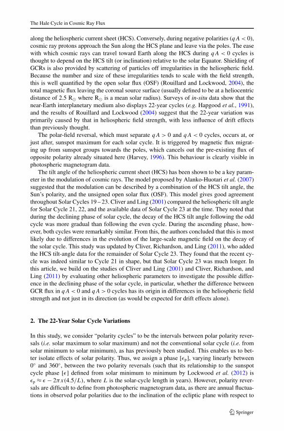
Figure 5 Heliospheric magnetic-field magnitude [|B∗|] and open solar flux [OSF∗] reconstructed from ge-omagnetic data, along with the monthly sunspot number and the monthly standard deviation of the dailysunspot number. This plot considers the space-age period (1965 – 2012). The red curves show qA < 0 po-larity cycles for each parameter, whereas the blue curves show qA > 0 cycles. The left column shows theraw data, the middle column shows the data normalised to the maximum and minimum values, and the rightcolumn gives the mean and standard deviations of the polarity cycles.

standard deviations (right column) of the qA < 0 and qA > 0 polarity cycles (in blue andred, respectively) determined using the sunspot method of defining εp. This analysis is givenfor (from top) |B∗| the heliospheric magnetic-field magnitude, and OSF∗ the open solar flux(where the asterisks denote that values are reconstructed from geomagnetic data), along withmonthly sunspot numbers and the monthly standard deviation of the daily sunspot number.

Figure 5 shows the space-age data only, whereas Figure 6 gives the pre-space-age data.As can be seen from Figure 5, the difference between the qA < 0 and qA > 0 cycles dur-ing the space age is still present in |B∗| and OSF∗. Because the reconstructed data havea yearly resolution, the data are binned more coarsely, with fewer data points averaged toproduce each data point, which may partly explain why the differences in |B∗| and OSF∗are slightly less pronounced than for |B| and OSF in Figure 4. The sunspot numbers andstandard deviations are also plotted at this yearly resolution and show the same trends asfound previously for the monthly averages. Note that the geomagnetic data do not cover thefinal 72◦ of the polarity-cycle phase. This is because the geomagnetic data are only availableup until June 2008, while in this study the main focus times are the declining phases of thesolar cycle.

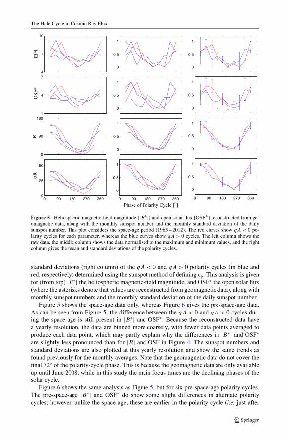
Figure 6 shows the same analysis as Figure 5, but for six pre-space-age polarity cycles.The pre-space-age |B∗| and OSF∗ do show some slight differences in alternate polaritycycles; however, unlike the space age, these are earlier in the polarity cycle (i.e. just after

S.R. Thomas et al.

Figure 6 Pre-space-age reconstructions of heliospheric magnetic-field magnitude [|B∗|] and open solar flux[OSF∗]; the sunspot number and standard deviation of daily sunspot number are also shown. The red curvesshow qA < 0 polarity cycles for each parameter, whereas the blue curves show qA > 0 cycles. The left col-umn shows the raw data, the middle column shows the normalised data, and the right column is a superposedepoch analysis.

solar maximum) and hence no longer coincident with the Hale Cycle differences in thecosmic-ray flux. Furthermore, the standard deviation of daily sunspot numbers with respectto the monthly averages does not show the same variation between alternate polarity cyclesin the pre-space-age data (in fact, the qA > 0 cycles give slightly higher mean values at therelevant εp than the qA < 0 cycles in Figure 5, but the difference is small compared to theerrors).

We now test the sensitivity of the results shown in Figures 5 and 6 to realistic variationson the start and end times of the polarity cycle (i.e. changes in the time of polarity rever-sal). Comparison of the polarity-reversal times determined from sunspot number and pho-tospheric magnetograph data (Figure 1) suggests a typical uncertainty of around 0.5 years.Therefore we performed a Monte Carlo analysis of the difference in heliospheric parame-ters in the qA < 0 and qA > 0 cycles to the varying the reversal times by half a year. Foreach variable shown in Figures 5 and 6 (i.e. the geomagnetic reconstructions of magnetic-field magnitude and OSF, the monthly sunspot number, and the sunspot variance) we usedrandom numbers to vary the start and end times of each cycle by 0.5 years with a chosenweighting of 50 % chance of no change in start and end time and 50 % of the reversal timechanging by 0.5 years (with an equal probability of moving backward or forward 0.5 years).For each set of new polarity reversal times, we repeated the same superposed-epoch analy-

The Hale Cycle in Cosmic Ray Flux

Figure 7 Sensitivity analysis of geomagnetic and sunspot data to varying the start and end dates by plus orminus 0.5 years. Each panel shows the difference between qA < 0 and qA > 0 polarity cycles of the followingparameters (from top): reconstructed magnetic-field intensity, reconstructed open solar flux, sunspot number,and sunspot variance. The green line shows the mean of all space-age cycles and the black line shows allpre-space-age cycles with the error bars representing the standard deviation of all cycles included in themean.

sis and computed the difference in the qA > 0 and qA < 0 parameters. We ran this process1 000 times to obtain a broad spread of cycle start and end times.

Figure 7 shows the difference in heliospheric parameters between the qA > 0 and qA < 0cycles, with the space age (pre-space age) in green (black). Shown from top to bottom aregeomagnetic reconstructions of the heliospheric magnetic field [|B∗|], the open solar flux[OSF∗], the sunspot number [R], and the sunspot variance [σR], as used in previous plots.Each parameter was averaged over all available cycles of each polarity and the differencesbetween the means for the qA < 0 and qA > 0 cycles are plotted. The green lines are theaverage behaviour of all space-age cycles and the black lines are all pre-space-age cycles.The error bars on each plot are plus or minus the standard deviation of all cycles included inthe mean of all samples.

For the heliospheric magnetic-field strength [|B∗|] (top panel) both the pre-space-agedata (black line) and the space-age data (green line) show a difference around εp = 100◦,which is larger than the error bars and so is considered significant. This difference is signif-icant at all phases of the declining phase of the sunspot cycle (εp < 100◦) for the pre-space-age data, but not for shortly after solar maximum in the space-age data. This means thatshortly after sunspot maximum, |B∗| during qA < 0 cycles is larger than for qA > 0 cyclesin the pre-space-age data, which is the opposite of the space-age data. The result that there

S.R. Thomas et al.

is no significant difference between the two polarity cycles for sunspot number [R] is foundnot to be sensitive to the start and end times of cycles used.

On the other hand, for both the OSF∗ and the sunspot number variability [σR], the resultholds when subjected to sensitivity testing; that is, the declining phases of the space-agecycles show an increase in these parameters during qA < 0 over qA > 0, but do not show adifference in pre-space-age data. This is shown as the peak in the space-age data above thepre-space age is more than zero by more than the error bar.

Another result to note is the difference at the start of the polarity cycle seen in the geo-magnetic |B∗| data. Here we see |B∗| during qA < 0 dominating |B∗| during qA > 0 duringpre-space-age cycles, but the opposite is true for space-age cycles. This result may warrantfurther work but is not seen in any other variable.

5. Discussion and Conclusions

As cosmic rays are modulated by the heliospheric magnetic field and heliospheric current-sheet tilt, the 11-year cycle is also seen in cosmic ray records. In addition to the solar cycle,cosmic ray time series display a strong 22-year Hale Cycle, which has been attributed todiffering drift patterns and diffusion (particularly at solar maximum) during positive andnegative solar field polarities (e.g. Jokipii, Levy, and Hubbard, 1977; Ferreira and Potgeiter,2004). It has been argued that this results in the earlier rise to the cosmic ray peak duringqA > 0 cycles than for qA < 0 cycles, and gives the time series a flat-topped and peakedappearance, respectively. However, an increasing number of results are not consistent withthis concept. For example, Richardson, Cane, and Wibberenz (1999) and Gil and Alanis(2008) have found that recurring decreases in cosmic ray fluxes were considerably strongerwhen qA > 0, whereas the drift theory suggests that they should be stronger for qA < 0,when cosmic rays should be entering by drifting inward along the HCS. In addition, otherstudies have found differences between qA > 0 and qA < 0 in the HCS tilt (Cliver andLing, 2001) and in open solar flux (Rouillard and Lockwood, 2004) that offer alternativeexplanations of the 22-year cycle in cosmic ray fluxes.

In this study, we separated space-age solar and heliospheric data into polarity cycles de-fined as intervals between polar solar-polarity reversals, thus approximately spanning solarmaximum to solar maximum.

The results show a significant difference in the behaviour of HCS inclination, helio-spheric magnetic-field magnitude, and open solar flux between qA > 0 cycles and qA < 0cycles. This difference is only significant during the first half of the polarity cycle, whichcorresponds to the declining phase of the solar cycle, the period responsible for a large partof the difference in GCR fluxes in the qA > 0 and qA < 0 cycles. The standard deviationin daily sunspot number also gives a significant difference between qA > 0 and qA < 0cycles during the same period, suggesting a greater prevalence of active longitudes duringthis phase of qA < 0 cycles. This agrees with the increased HCS inclination throughoutthis period. The presence of more active longitudes giving greater HCS inclination meansthat there will be regular fast/slow stream interfaces extending over broad latitudinal ranges,which was shown to be an effective way of shielding cosmic rays in a case study by Rouil-lard and Lockwood (2007).

We suggest that the 22-year cycle in GCR flux may be partly due to direct heliosphericmodulation, although drift effects (Jokipii, Levy, and Hubbard, 1977; Ferreira and Potgeiter,2004) will still play a role, particularly during the end of the polarity cycle (i.e. the rise phaseof the solar cycle), when differences in heliospheric parameters are less apparent. Of course,

The Hale Cycle in Cosmic Ray Flux

while changes in heliospheric structure are coincident with the differing behaviour in cosmicray flux in alternate polarity cycles, it still remains to be shown that they are of sufficientmagnitude to effect the required modulation. To do this will, however, require a significantmodelling effort.

The above conclusions relate to the space-age era for which there are in-situ observationsof interplanetary parameters and magnetograph data from which the start and end times ofthe polarity cycle and the HCS tilt index can be derived. Because these data have been takenduring a grand solar maximum (Lockwood, Rouillard, and Finch, 2009), the conclusionsmight not necessarily have been valid in the less active times prior to the grand maximum. Totest this, the open solar flux and near-Earth magnetic field reconstructed from geomagneticactivity data were used, employing the sunspot number variations to define the start and endtimes of the polarity cycle. The data were divided into the space-age era (1965 and aftercorresponding to the first study) and pre-space-age data before 1965.

The reconstructed data from the space-age era supported the above findings of the studyusing direct observations, but we also noted that the differences between polarity cyclesare considerably smaller before the space age. Using geomagnetic reconstructions of helio-spheric magnetic-field magnitude and open solar flux, it was shown that for the period of1905 – 1965, the opposite polarities do not give such differing patterns during the decliningphase of the solar cycle. In particular, the variability in sunspot numbers is greatly reduced.One source of uncertainty that we addressed is that before the space age we have to use thesunspot number variation to define the start and end time of the polarity cycles. A sensitiv-ity study that added the uncertainty in these inferred times showed that the result is robustfor the open solar flux [OSF] and the variability of the sunspot number [σR]. However, thisuncertainty means that we cannot be certain that the polarity effect on the near-Earth he-liospheric field strength (at the phase of the polarity cycle when the polarity effect on GCRis greatest in the space-age era) is different in the pre-space-age data compared with thespace-age era.

The data suggest that the polarity-dependent effect on cosmic rays before the recent grandsolar maximum was most likely restricted to the drift effects and was not as marked as it hasbeen in recent data. This is consistent with cosmogenic isotope data, which, in general, donot show strong 22-year Hale cycle variations (Usoskin, 2008).

Acknowledgements We are grateful to the Space Physics Data Facility (SPDF) of NASA’s Goddard SpaceFlight Centre for combining the data into the OMNI 2 data set, which was obtained via the GSFC/SPDF OM-NIWeb interface at omniweb.gsfc.nasa.gov and to the Marshall Space Flight Centre for the Sunspot Numberdata obtained from MSFC at solarscience.msfc.nasa.gov/greenwch.shtml. We also thank the Bartol ResearchInstitute of the University of Delaware for the neutron-monitor data from McMurdo, which is supported byNSF grant ATM-0527878 and J.T. Hoeksema of Stanford University for WSO magnetograms. The work ofSRT is supported by a studentship from the UK’s Natural Environment Research Council (NERC).

References

Ahluwalia, H.S., Ygbuhay, R.C.: 2010, Status of Galactic Cosmic Ray Recovery from Sunspot Cycle 23Modulation CP-1216, AIP, New York, 699 – 702.

Alanko-Huotari, K., Usoskin, I.G., Mursala, K., Kovaltsov, G.A.: 2007, Cyclic variations of the heliospherictilt angle and cosmic ray modulation. Adv. Space Res. 40, 1064 – 1069.

Babcock, H.D.: 1959, The Sun’s polar magnetic field. Astrophys. J. 130, 364 – 366. ADS:1959ApJ...130..364B, doi:10.1086/146726.

Babcock, H.W., Babcock, H.D.: 1955, The Sun’s magnetic field 1952 – 1954. Astrophys. J. 121, 349.Beer, J., Vonmoos, M., Muscheler, R.: 2006, Solar variability over the past several millennia. Space Sci. Rev.

125, 67 – 79.

S.R. Thomas et al.

Berdyugina, S.V., Usoskin, I.G.: 2003, Active longitudes in sunspot activity: century scale persistence. Astron.Astrophys. 405, 1121 – 1128.

Bieber, J.W., Clem, J.M., Duldig, M.L., Evenson, P.A., Humble, J.E., Pyle, R.: 2004, Latitudinal surveyobservations of neutron monitor multiplicity. J. Geophys. Res. 109. doi:10.1029/2004JA010493.

Chernosky, E.J.: 1966, Double sunspot-cycle variation in terrestrial magnetic activity. J. Geophys. Res. 71,965.

Cliver, E.W., Ling, A.G.: 2001, 22 year patterns in the relationship of sunspot number and tilt angle to cosmic-ray intensity. Astrophys. J. 551, 189 – 192.

Cliver, E.W., Richardson, I.G., Ling, A.G.: 2011, Solar drivers of 11-year and long-term cosmic ray modula-tion. Space Sci. Rev. doi:10.1007/s11214-011-9746-3.

Ellis, W.: 1899, On the relation between magnetic disturbances and the period of solar spot frequency. Mon.Not. Roy. Astron. Soc. 60, 142 – 157.

Ferreira, S.E.S., Potgeiter, M.S.: 2004, Long-term cosmic-ray modulation in the heliosphere. Astrophys. J.603, 744 – 752.

Forbush, S.E.: 1954, Worldwide cosmic ray variations, 1937 – 1952. J. Geophys. Res. 59, 525 – 542.Gil, A., Alanis, M.V.: 2008, On the energy spectrum of the 27-day variation of the galactic cosmic ray inten-

sity. In: Proc. 30th Internat. Cosmic Ray (ICRC07) Conf. 1 (SH), 601 – 604.Hale, G.E., Nicholson, S.B.: 1925, The law of Sun-spot polarity. Astrophys. J. 62, 270 – 300.Hapgood, M.A.: 2010, Towards a scientific understanding of the risk from extreme space weather. Adv. Space

Res. 47, 2059 – 2072.Hapgood, M.A., Bowe, G., Lockwood, M., Willis, D.M., Tulunay, Y.: 1991, Variability of the interplanetary

magnetic field at 1 A.U. over 24 years: 1963 – 1986. Planet. Space Sci. 39, 411 – 423.Harvey, K.L.: 1996, Large scale patterns of magnetic activity and the solar cycle. Bull. Am. Astron. Soc. 28,

867.Hathaway, D.H.: 2012, The solar cycle. Living Rev. Solar Phys. 7, 1. doi:10.12942/lrsp-2010-1.Hathaway, D.H., Wilson, R.M., Reichmann, E.J.: 1994, The shape of the sunspot cycle. Solar Phys. 151,

177 – 190. ADS:1994SoPh..151..177H, doi:10.1007/BF00654090.Jokipii, J.R., Thomas, B.: 1981, Effects of drift on the transport of cosmic rays IV. Modulation by a wavy

interplanetary current sheet. Astrophys. J. 243, 1115 – 1122.Jokipii, J.R., Levy, E.H., Hubbard, W.B.: 1977, Effects of particle drift on cosmic-ray transport. I. General

properties, application to solar modulation. Astrophys. J. 213, 861 – 868.King, J.H., Papitashvili, N.E.: 2005, Solar wind spatial scales in and comparisons of hourly wind and ACE

plasma and magnetic field data. J. Geophys. Res. 110. doi:10.1029/2004JA010649.Lockwood, M.: 2003, Twenty-three cycles of changing open solar magnetic flux. J. Geophys, Res. 108.

doi:10.1029/2002JA009431.Lockwood, M.: 2010, Solar change and climate: an update in the light of the current exceptional solar mini-

mum. Proc. Roy. Soc. A 466, 303 – 329.Lockwood, M., Owens, M.J.: 2011, Centennial changes in the heliospheric magnetic field and open solar flux:

the consensus view from geomagnetic data and cosmogenic isotopes and its implications. J. Geophys,Res. 116. doi:10.1029/2010JA016220.

Lockwood, M., Rouillard, A.P., Finch, I.D.: 2009, The rise and fall of open solar flux during the current grandsolar maximum. Astrophys. J. 700, 937 – 944.

Lockwood, M., Owens, M.J., Barnard, L., Davis, C.J., Thomas, S.R.: 2012, What is the Sun up to? Astron.Geophys. 53, 3.9 – 3.15.

McCracken, K.G., McDonald, F.B., Beer, J., Raisbeck, G., Yiou, F.: 2004, A phenomenological studyof the long-term cosmic ray modulation, 850 – 1958 AD. J. Geophys, Res. 109. doi:10.1029/2004JA010685.

Mewaldt, R., Davis, A., Lave, K., Leske, R., Stone, E., Wiedenbeck, M., Binns, W., Christian, E., Cum-mings, A., De Nolfo, G., Israel, M., Labrador, A., Von Rosenvinge, T.: 2010, Record-setting cosmic rayintensities in 2009 and 2010. Astrophys. J. Lett. 723, L1 – L6.

Owens, M.J., Crooker, N.U., Lockwood, M.: 2011, How is open solar flux lost over the solar cycle? J. Geo-phys. Res. 116. doi:10.1029/2011JA016039.

Owens, M.J., Lockwood, M., Barnard, L., Davis, C.J.: 2011, Solar cycle 24: implications for energetic parti-cles and long-term space climate change. Geophys. Res. Lett. 38, 19106.

Parker, E.N.: 1965, The passage of energetically charged particles through interplanetary space. Planet. SpaceSci. 13, 9 – 49.

Potgieter, M.S.: 1995, The time-dependent transport of cosmic rays in the heliosphere. Astrophys. Space Sci.116. doi:10.1029/2010JA016220.

Richardson, I.G., Cane, H.V., Wibberenz, G.: 1999, A 22-year dependence in the size of near-ecliptic coro-tating cosmic ray depressions during five solar minima. J. Geophys. Res. 104, 12549.

The Hale Cycle in Cosmic Ray Flux

Rouillard, A., Lockwood, M.: 2004, Oscillations in the open solar magnetic flux with a period of 1.68 years:imprint on galactic cosmic rays and implications for heliospheric shielding. Ann. Geophys. 22, 4381 –4395.

Rouillard, A., Lockwood, M.: 2007, The latitudinal effect of co-rotating interaction regions on galac-tic cosmic rays. Solar Phys. 245, 191 – 206. ADS:2007SoPh..245..191R, doi:10.1007/s11207-007-9019-1.

Ruzmaikin, A.A., Feynman, J., Neugebauer, M., Smith, E.J.: 2000, On the nature and persistence of preferredlongitudes of solar activity. Bull. Am. Astron. Soc. 32, 835.

Schwabe, M.: 1843, Die Sonne. Von Herrn Hofrath Schwabe. Astron. Nachr. 20, 283.Smith, E.J.: 1990, The heliospheric current sheet and modulation of galactic cosmic rays. J. Geophys. Res.

95, 18731 – 18743.Smith, E.J., Thomas, E.J.: 1986, Latitudinal extent of the heliospheric current sheet and modulation of galactic

cosmic rays. J. Geophys. Res. 91, 2933 – 2942.Solanki, S.K., Usoskin, I.G., Kromer, B., Schuessler, M., Beer, J.: 2004, Unusual acticity of the Sun during

recent decades compared to the previous 11 000 years. Nature 431, 1084 – 1087.Svalgaard, L., Cliver, E.W., Kamide, Y.: 2005, Cycle 24: smallest in 100 years? Geophys. Res. Lett. 32.

doi:10.1029/2004GL021664.Usoskin, I.G.: 2008, A history of solar activity over millennia. Living Rev. Solar Phys. 5, 1 – 60. doi:10.12942/

lrsp-2008-3.Usoskin, I.G., Bazilevskaya, G.A., Kovaltsov, G.A.: 2011, Solar modulation parameter for cosmic rays since

1936 reconstructed from ground-based neutron monitors and Ionization chambers. J. Geophys. Res. 116.doi:10.1029/2010JA016105.

Van Allen, J.A.: 2000, On the modulation of galactic cosmic ray intensity during solar activity cycles 19, 20,21, 22 and early 23. Geophys. Res. Lett. 27, 2453 – 2456.

Waldmeier, M.: 1935, Neue Eigenschaften der Sonnenfleckenkurve. Astron. Mitt. Zurich 14, 105 – 130.Wang, Y.M., Sheeley Jr., N.R., Rouillard, A.P.: 2006, Role of the Sun’s nonaxisymmetric open flux in cosmic

ray modulation. Astrophys. J. 644, 638.Webber, W.R., Lockwood, J.A.: 1988, Characteristics of the 22-year modulation of cosmic rays as seen by

neutron monitors. J. Geophys. Res. 93, 8735 – 8740.