Embed Size (px)
Citation preview
The 2014 OCB Summer Science Workshop The Coupled North Atlantic-Arctic System: Processes and Dynamics
(Mon. July 21) Woods Hole Oceanographic Institution
Quissett Campus, Clark 507, Woods Hole, MA.
8/6/2014 The 2014 OCB Summer Workshop 1
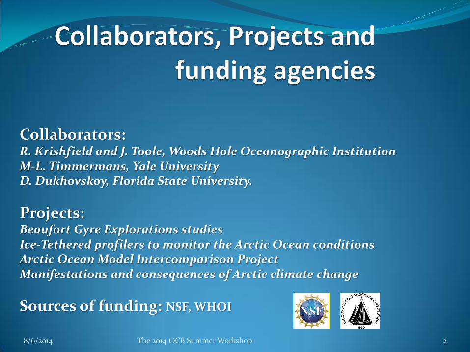
Collaborators: R. Krishfield and J. Toole, Woods Hole Oceanographic Institution M-L. Timmermans, Yale University D. Dukhovskoy, Florida State University.
Projects: Beaufort Gyre Explorations studies Ice-Tethered profilers to monitor the Arctic Ocean conditions Arctic Ocean Model Intercomparison Project Manifestations and consequences of Arctic climate change
Sources of funding: NSF, WHOI
8/6/2014 The 2014 OCB Summer Workshop 2

NBC News Learn program in partnership with the National Science Foundation prepared a 5-minute film
describing our Beaufort Gyre exploration project hypothesis, objectives, tasks and preliminary results.
This film is located at the Beauofort Gyre website www.whoi.edu/beaufortgyre.
8/6/2014 The 2014 OCB Summer Workshop 3
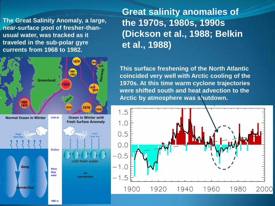
The Great Salinity Anomaly, a large,
near-surface pool of fresher-than-
usual water, was tracked as it
traveled in the sub-polar gyre
currents from 1968 to 1982.
This surface freshening of the North Atlantic
coincided very well with Arctic cooling of the
1970s. At this time warm cyclone trajectories
were shifted south and heat advection to the
Arctic by atmosphere was shutdown.
Cold air
Surface
Warm
deep
water
1000 m
Great salinity anomalies of
the 1970s, 1980s, 1990s
(Dickson et al., 1988; Belkin
et al., 1988)

Arctic Ocean - largest freshwater reservoir
45,000 km3
17,300 km3
2,800 km3
3,800 km3
12,200 km3
2,900 km3
3,400 km3
5,300 km3
4,000 km3
77 km3
Aagaard and
Carmack, 1989 And the oceanic Beaufort
Gyre (BG) of the Canadian
Basin is the largest
freshwater reservoir in the
Arctic Ocean (Aagaard and
Carmack, 1989). Freshwater
content: calculated relative to
salinity 34.80 according to
Aagaard K. and E. Carmack,
JGR, vol. 94, C10, 14,495-
14,498,1989. The total
freshwater content of the Arctic
Ocean based on the data from
the 1970s is about 80,000
cubic km.
8/6/2014 The 2014 OCB Summer Workshop 6
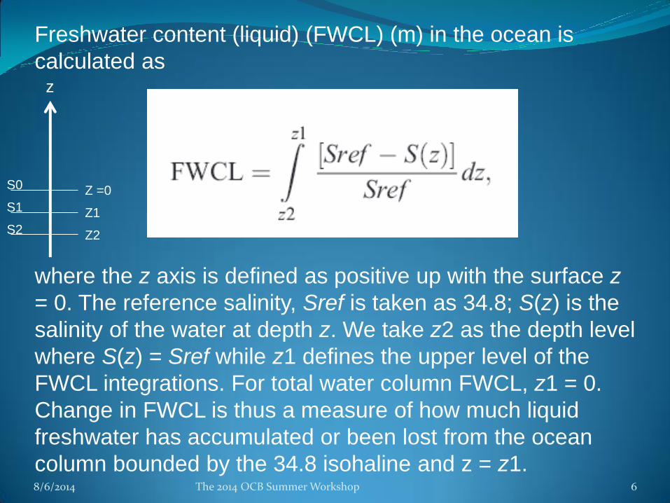
Freshwater content (liquid) (FWCL) (m) in the ocean is
calculated as
where the z axis is defined as positive up with the surface z
= 0. The reference salinity, Sref is taken as 34.8; S(z) is the
salinity of the water at depth z. We take z2 as the depth level
where S(z) = Sref while z1 defines the upper level of the
FWCL integrations. For total water column FWCL, z1 = 0.
Change in FWCL is thus a measure of how much liquid
freshwater has accumulated or been lost from the ocean
column bounded by the 34.8 isohaline and z = z1.
z
Z =0
Z1
Z2
S0
S1
S2
8/6/2014 The 2014 OCB Summer Workshop 7
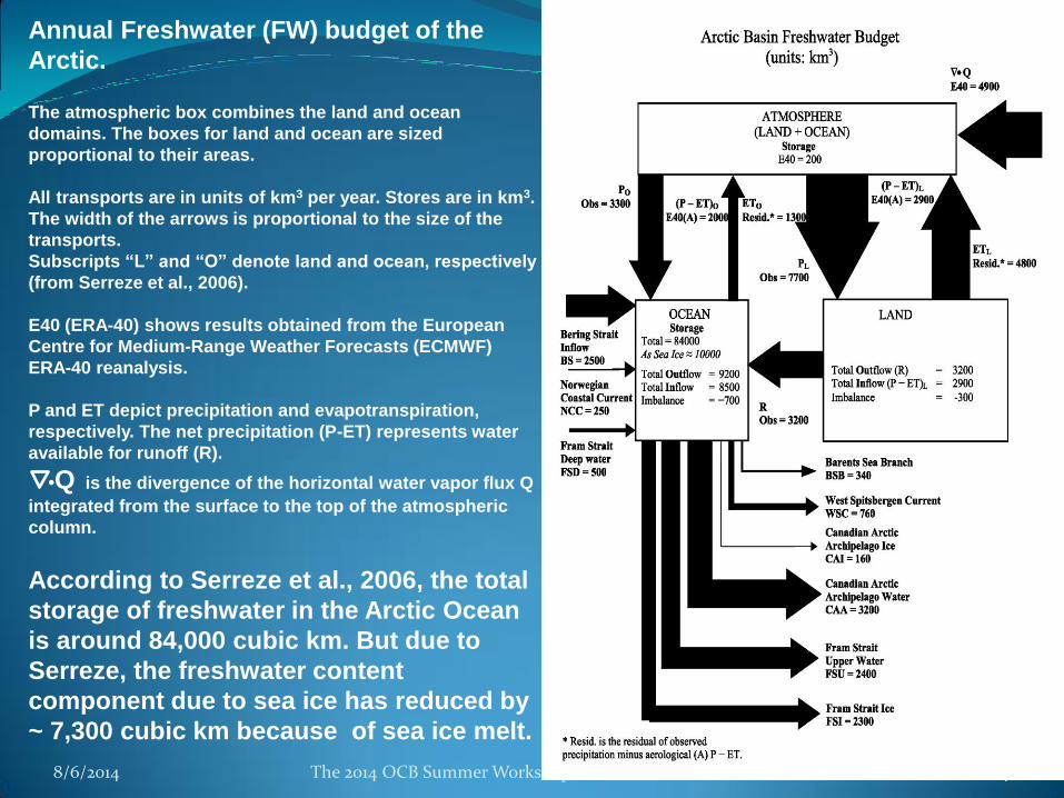
Annual Freshwater (FW) budget of the
Arctic. The atmospheric box combines the land and ocean
domains. The boxes for land and ocean are sized
proportional to their areas.
All transports are in units of km3 per year. Stores are in km3.
The width of the arrows is proportional to the size of the
transports.
Subscripts “L” and “O” denote land and ocean, respectively
(from Serreze et al., 2006).
E40 (ERA-40) shows results obtained from the European
Centre for Medium-Range Weather Forecasts (ECMWF)
ERA-40 reanalysis.
P and ET depict precipitation and evapotranspiration,
respectively. The net precipitation (P-ET) represents water
available for runoff (R).
•Q is the divergence of the horizontal water vapor flux Q
integrated from the surface to the top of the atmospheric
column.
According to Serreze et al., 2006, the total
storage of freshwater in the Arctic Ocean
is around 84,000 cubic km. But due to
Serreze, the freshwater content
component due to sea ice has reduced by
~ 7,300 cubic km because of sea ice melt.

8/6/2014 The 2014 OCB Summer Workshop 8
Annual Freshwater (FW) budget of the
Arctic. The atmospheric box combines the land and ocean
domains. The boxes for land and ocean are sized
proportional to their areas.
All transports are in units of km3 per year. Stores are in km3.
The width of the arrows is proportional to the size of the
transports.
Subscripts “L” and “O” denote land and ocean, respectively
(from Serreze et al., 2006).
E40 (ERA-40) shows results obtained from the European
Centre for Medium-Range Weather Forecasts (ECMWF)
ERA-40 reanalysis.
P and ET depict precipitation and evapotranspiration,
respectively. The net precipitation (P-ET) represents water
available for runoff (R).
•Q is the divergence of the horizontal water vapor flux Q
integrated from the surface to the top of the atmospheric
column.
According to Serreze et al., 2006, the total
storage of freshwater in the Arctic Ocean
is around 84,000 cubic km. But due to
Serreze, the freshwater content
component due to sea ice has reduced by
~ 7,300 cubic km because of sea ice melt.
Storage: Ocean: 84,000,
Ice: 10,000
cubic km.
8/6/2014 The 2014 OCB Summer Workshop 9
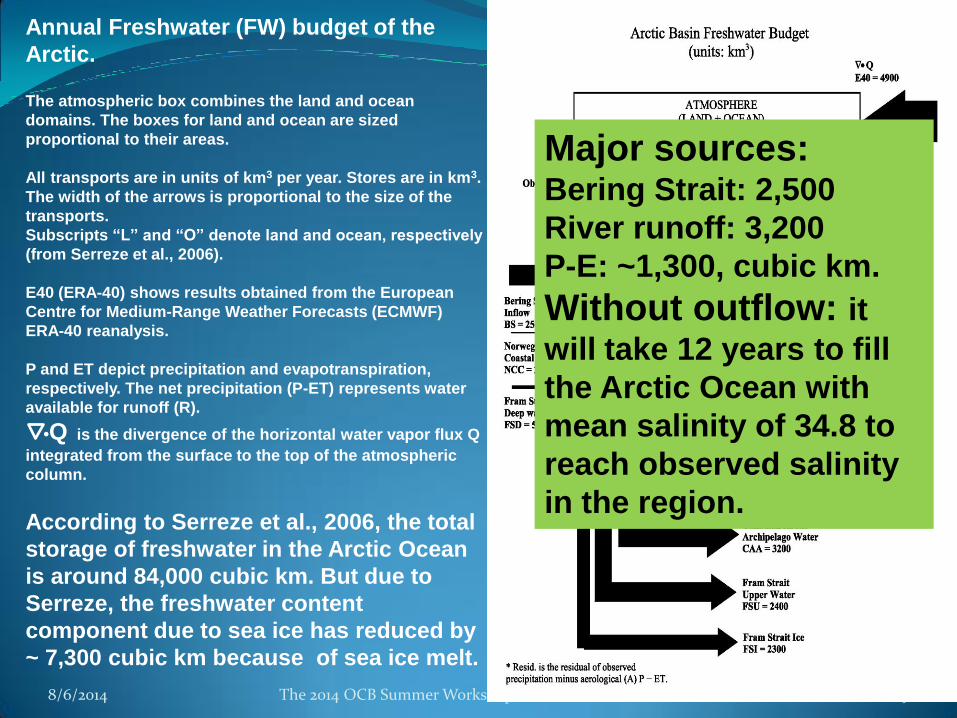
Annual Freshwater (FW) budget of the
Arctic. The atmospheric box combines the land and ocean
domains. The boxes for land and ocean are sized
proportional to their areas.
All transports are in units of km3 per year. Stores are in km3.
The width of the arrows is proportional to the size of the
transports.
Subscripts “L” and “O” denote land and ocean, respectively
(from Serreze et al., 2006).
E40 (ERA-40) shows results obtained from the European
Centre for Medium-Range Weather Forecasts (ECMWF)
ERA-40 reanalysis.
P and ET depict precipitation and evapotranspiration,
respectively. The net precipitation (P-ET) represents water
available for runoff (R).
•Q is the divergence of the horizontal water vapor flux Q
integrated from the surface to the top of the atmospheric
column.
According to Serreze et al., 2006, the total
storage of freshwater in the Arctic Ocean
is around 84,000 cubic km. But due to
Serreze, the freshwater content
component due to sea ice has reduced by
~ 7,300 cubic km because of sea ice melt.
Major sources: Bering Strait: 2,500
River runoff: 3,200
P-E: ~1,300, cubic km.
Without outflow: it will take 12 years to fill
the Arctic Ocean with
mean salinity of 34.8 to
reach observed salinity
in the region.
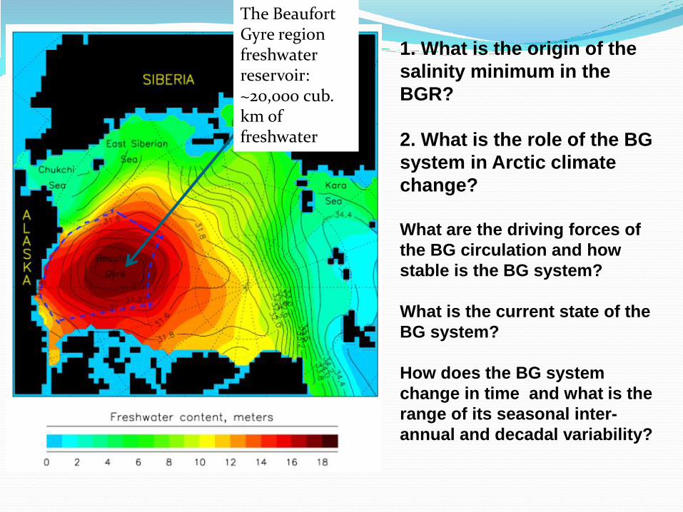
The Beaufort Gyre region freshwater reservoir: ~20,000 cub. km of freshwater
1. What is the origin of the
salinity minimum in the
BGR?
2. What is the role of the BG
system in Arctic climate
change?
What are the driving forces of
the BG circulation and how
stable is the BG system?
What is the current state of the
BG system?
How does the BG system
change in time and what is the
range of its seasonal inter-
annual and decadal variability?
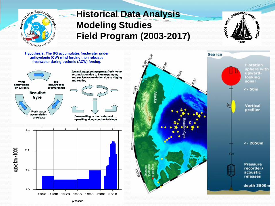
Historical Data Analysis
Modeling Studies
Field Program (2003-2017)
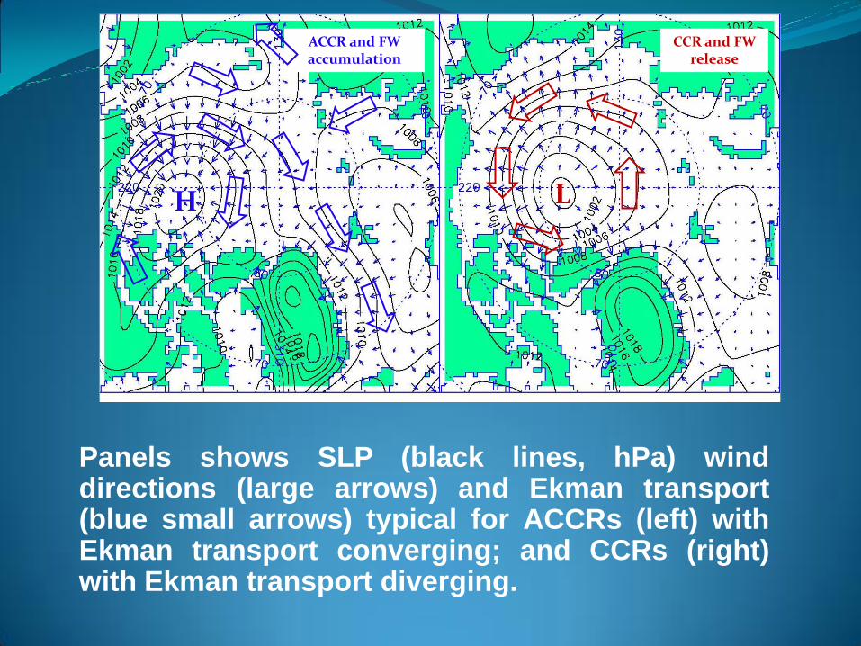
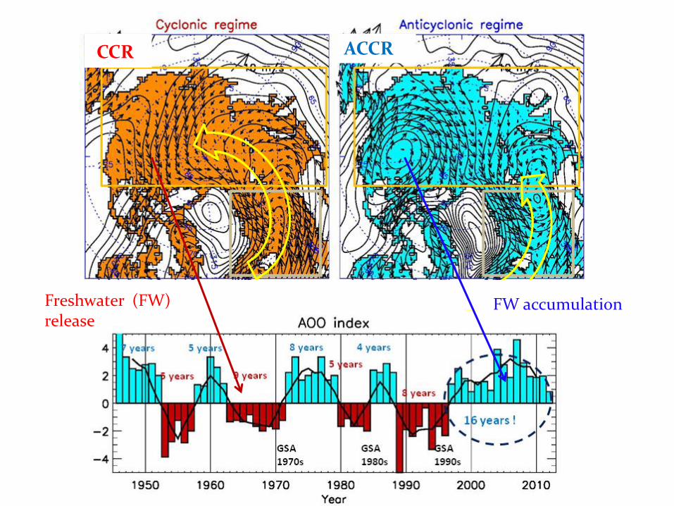
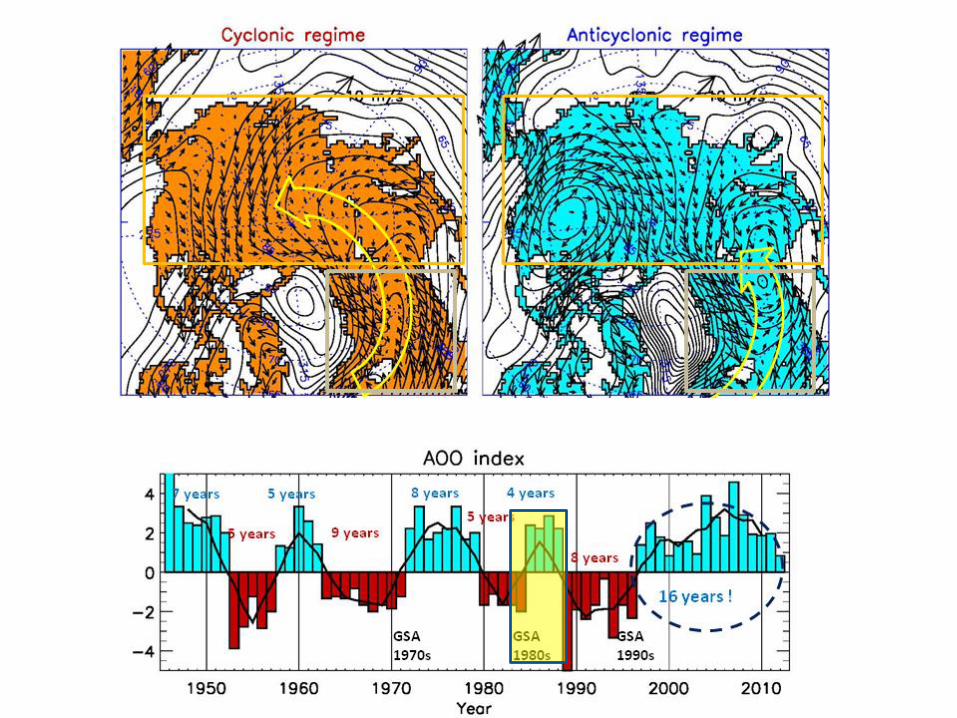
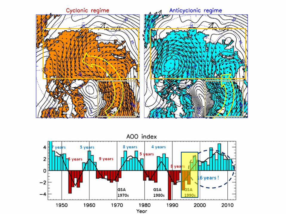
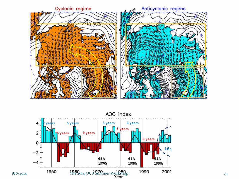
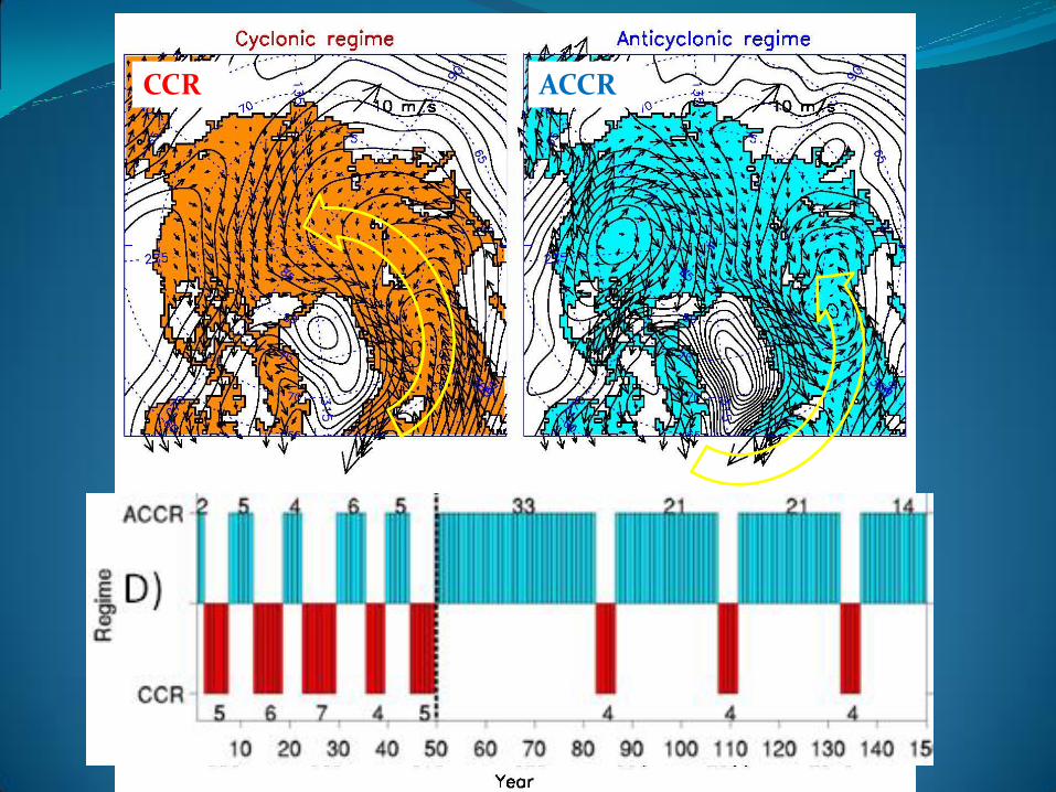
Panels shows SLP (black lines, hPa) wind directions (large arrows) and Ekman transport (blue small arrows) typical for ACCRs (left) with Ekman transport converging; and CCRs (right) with Ekman transport diverging.
ACCR and FW accumulation
CCR and FW release
L H
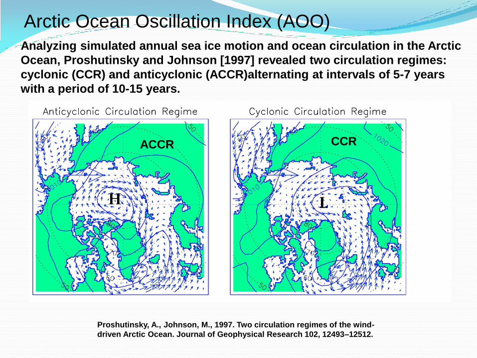
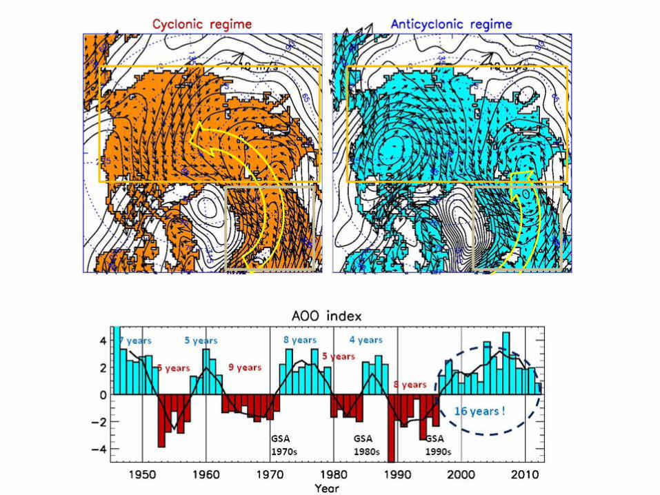
Arctic Ocean Oscillation Index (AOO)
Analyzing simulated annual sea ice motion and ocean circulation in the Arctic
Ocean, Proshutinsky and Johnson [1997] revealed two circulation regimes:
cyclonic (CCR) and anticyclonic (ACCR)alternating at intervals of 5-7 years
with a period of 10-15 years.
H
L L
L
ACCR CCR
Proshutinsky, A., Johnson, M., 1997. Two circulation regimes of the wind-
driven Arctic Ocean. Journal of Geophysical Research 102, 12493–12512.
H L
ACCR CCR
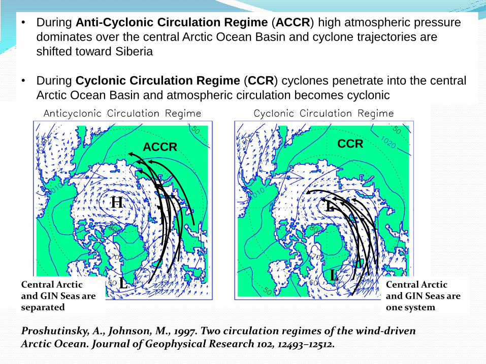
Central Arctic and GIN Seas are separated
Central Arctic and GIN Seas are one system
• During Anti-Cyclonic Circulation Regime (ACCR) high atmospheric pressure
dominates over the central Arctic Ocean Basin and cyclone trajectories are
shifted toward Siberia
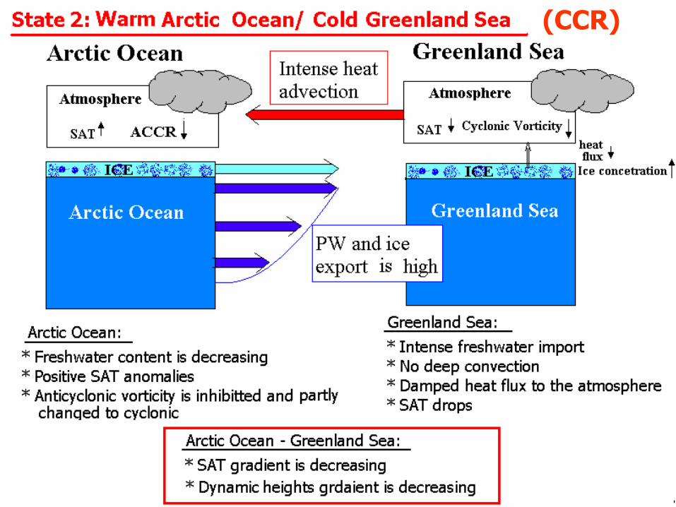
• During Cyclonic Circulation Regime (CCR) cyclones penetrate into the central
Arctic Ocean Basin and atmospheric circulation becomes cyclonic
Proshutinsky, A., Johnson, M., 1997. Two circulation regimes of the wind-driven Arctic Ocean. Journal of Geophysical Research 102, 12493–12512.
H
L
L
L
ACCR CCR
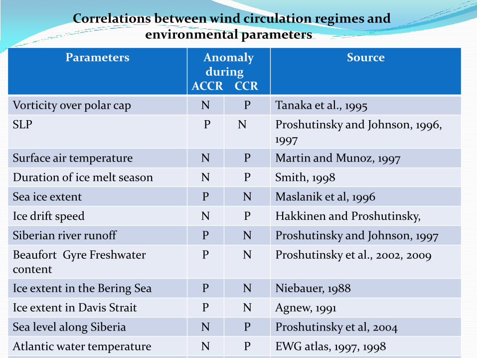
Correlations between wind circulation regimes and environmental parameters
Parameters Anomaly during ACCR CCR
Source
Vorticity over polar cap N P Tanaka et al., 1995
SLP P N Proshutinsky and Johnson, 1996, 1997
Surface air temperature N P Martin and Munoz, 1997
Duration of ice melt season N P Smith, 1998
Sea ice extent P N Maslanik et al, 1996
Ice drift speed N P Hakkinen and Proshutinsky,
Siberian river runoff P N Proshutinsky and Johnson, 1997
Beaufort Gyre Freshwater content
P N Proshutinsky et al., 2002, 2009
Ice extent in the Bering Sea P N Niebauer, 1988
Ice extent in Davis Strait P N Agnew, 1991
Sea level along Siberia N P Proshutinsky et al, 2004
Atlantic water temperature N P EWG atlas, 1997, 1998
Atlantic water salinity N P EWG atala, 1997, 1998
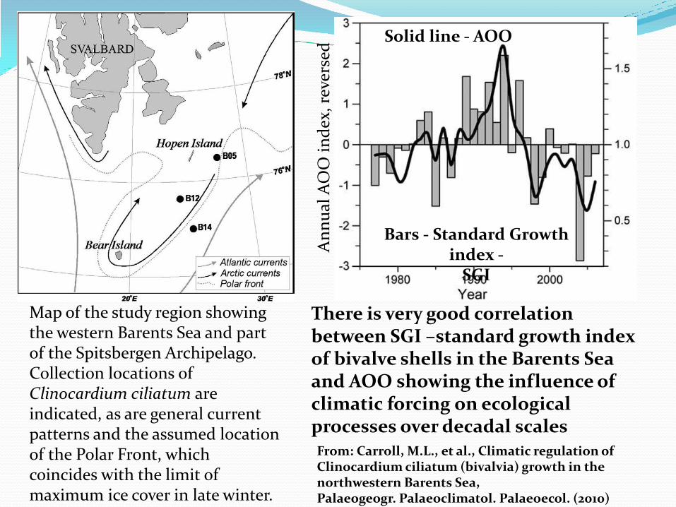
Map of the study region showing the western Barents Sea and part of the Spitsbergen Archipelago. Collection locations of Clinocardium ciliatum are indicated, as are general current patterns and the assumed location of the Polar Front, which coincides with the limit of maximum ice cover in late winter.
From: Carroll, M.L., et al., Climatic regulation of Clinocardium ciliatum (bivalvia) growth in the northwestern Barents Sea, Palaeogeogr. Palaeoclimatol. Palaeoecol. (2010)
An
nu
al A
OO
in
dex
, re
vers
ed
Bars - Standard Growth index -
SGI
Solid line - AOO
There is very good correlation between SGI –standard growth index of bivalve shells in the Barents Sea and AOO showing the influence of climatic forcing on ecological processes over decadal scales
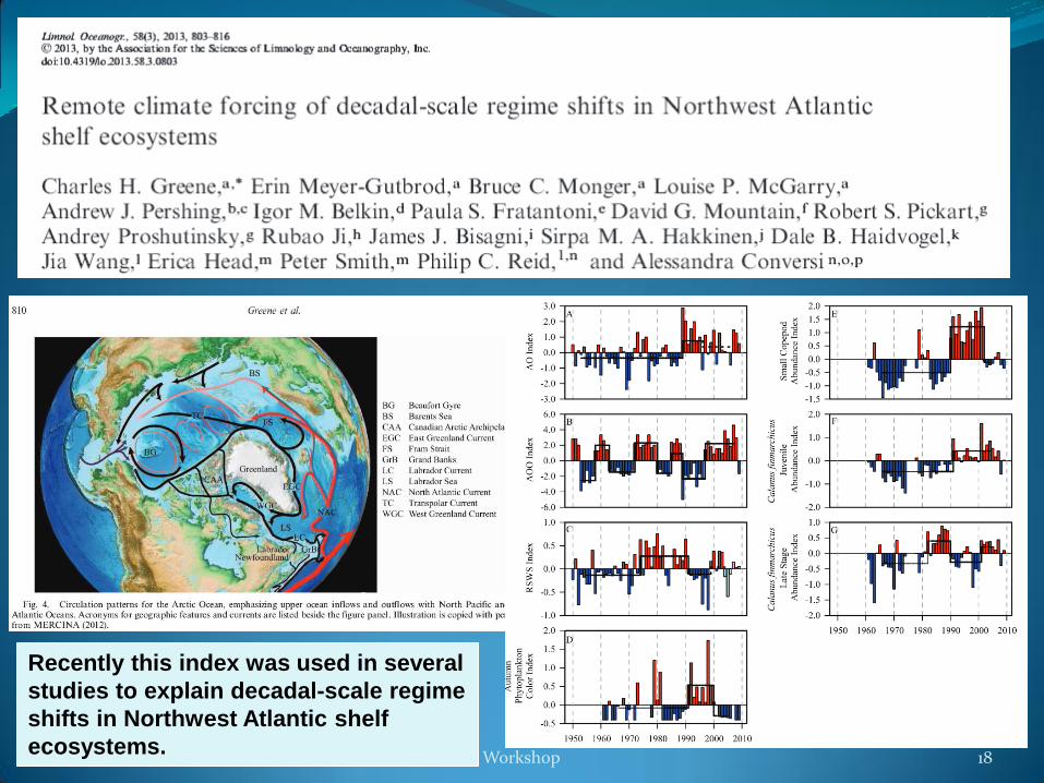
8/6/2014 The 2014 OCB Summer Workshop 18
Recently this index was used in several
studies to explain decadal-scale regime
shifts in Northwest Atlantic shelf
ecosystems.
CCR ACCR
Freshwater (FW) release
FW accumulation

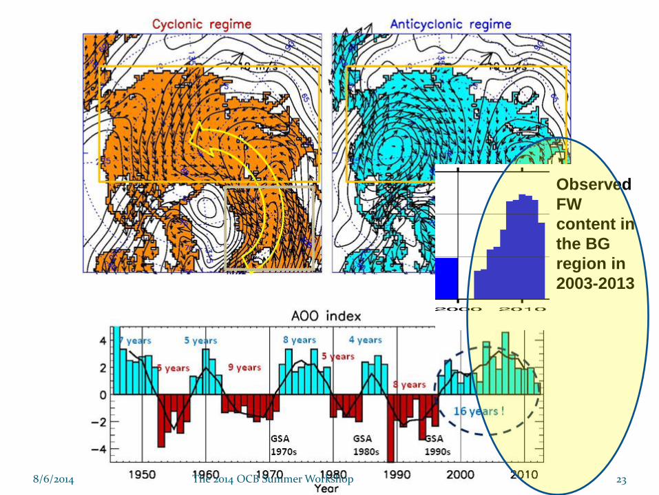
8/6/2014 The 2014 OCB Summer Workshop 23
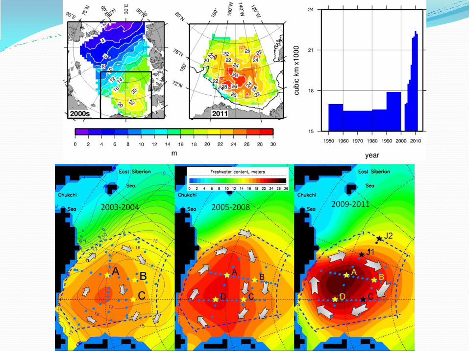
Observed
FW
content in
the BG
region in
2003-2013
• Our observations show that in the period 2003-2013 the BG region accumulated more than 5000 cubic km of freshwater, an increase of approximately 25% relative to the climatology of the 1970s.
• A possible FW release from the Arctic of this magnitude is enough to cause a salinity anomaly in the North Atlantic with magnitude comparable to the Great Salinity Anomaly (GSA) of the 1970s. GSAs can influence global climate by inhibiting deep wintertime convection that in turn may reduce the ocean meridional overturning circulation. In this sense, the BG FW reservoir is a “ticking time bomb” for climate.
• However, it is unclear whether the Arctic climate may have exceeded a "tipping point" where the freshwater will continue to accumulate and exceed anything observed in the past.
8/6/2014 The 2014 OCB Summer Workshop 24
8/6/2014 The 2014 OCB Summer Workshop 25
8/6/2014 The 2014 OCB Summer Workshop 26
Hypothesis
• Arctic Ocean – Greenland Sea form closed atmosphere-ice-ocean climatic system with auto-oscillatory behavior between two climate states with quasi-decadal periodicity
• The system is characterized by two opposite states: (1) ACCR - a cold Arctic and warm Greenland Sea region; (2) CCR - a warm Arctic and cold Greenland Sea region.
• Freshwater and heat fluxes regulate the regime shift in the system
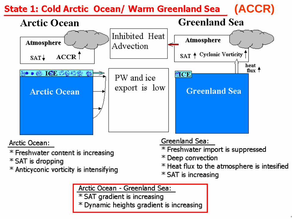
(ACCR)
(CCR)
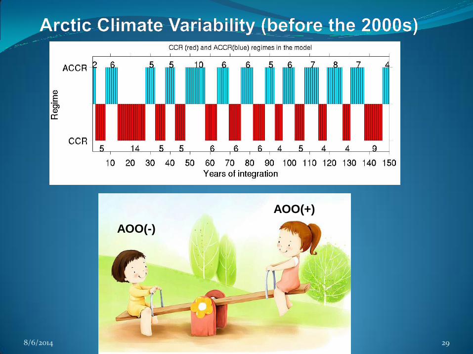
8/6/2014 The 2014 OCB Summer Workshop 29
AOO(-)
AOO(+)
8/6/2014 The 2014 OCB Summer Workshop 30
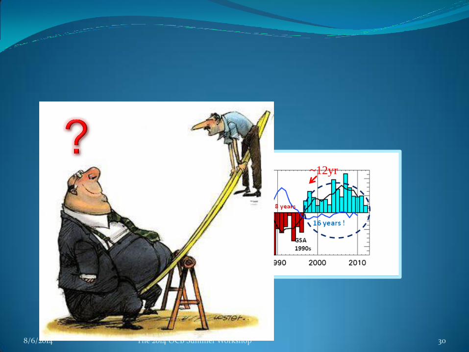
~10yr ~12yr
AOO (+)
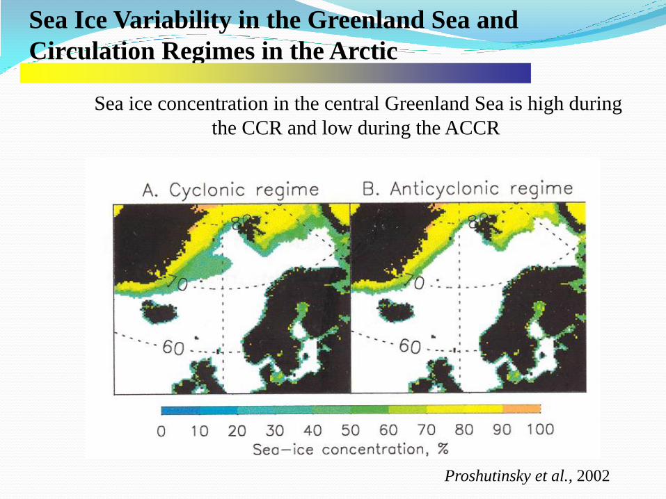
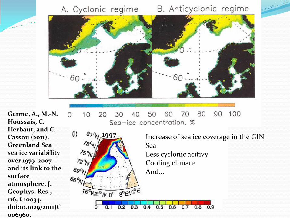
Sea Ice Variability in the Greenland Sea and
Circulation Regimes in the Arctic
Sea ice concentration in the central Greenland Sea is high during
the CCR and low during the ACCR
Proshutinsky et al., 2002
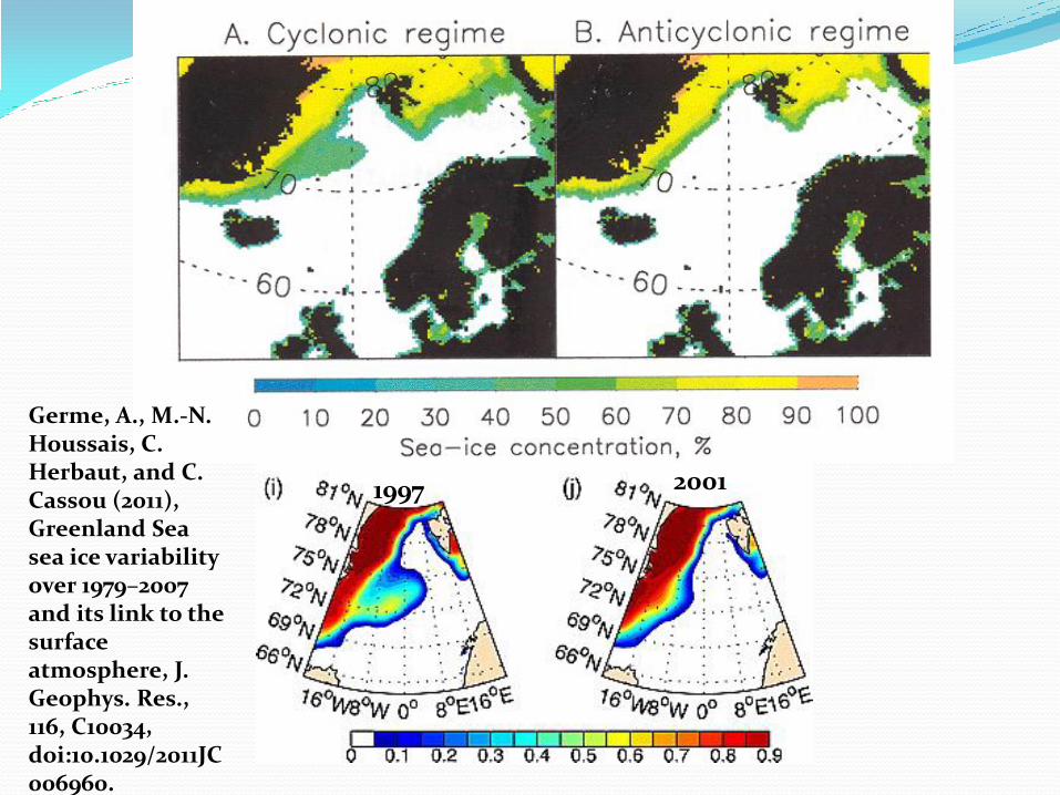
1997 2001
Germe, A., M.-N. Houssais, C. Herbaut, and C. Cassou (2011), Greenland Sea sea ice variability over 1979–2007 and its link to the surface atmosphere, J. Geophys. Res., 116, C10034, doi:10.1029/2011JC006960.
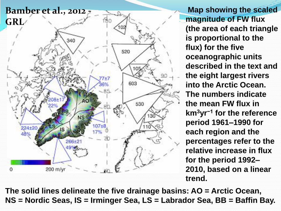
Map showing the scaled
magnitude of FW flux
(the area of each triangle
is proportional to the
flux) for the five
oceanographic units
described in the text and
the eight largest rivers
into the Arctic Ocean.
The numbers indicate
the mean FW flux in
km3yr−1 for the reference
period 1961–1990 for
each region and the
percentages refer to the
relative increase in flux
for the period 1992–
2010, based on a linear trend.
The solid lines delineate the five drainage basins: AO = Arctic Ocean,
NS = Nordic Seas, IS = Irminger Sea, LS = Labrador Sea, BB = Baffin Bay.
Bamber et al., 2012 - GRL
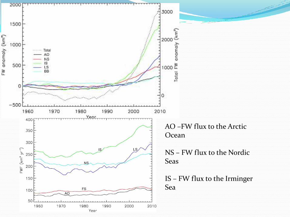
AO –FW flux to the Arctic Ocean NS – FW flux to the Nordic Seas IS – FW flux to the Irminger Sea

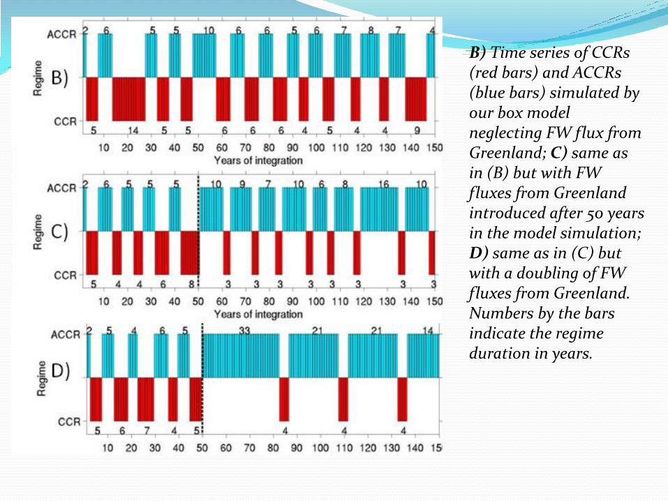
B) Time series of CCRs (red bars) and ACCRs (blue bars) simulated by our box model neglecting FW flux from Greenland; C) same as in (B) but with FW fluxes from Greenland introduced after 50 years in the model simulation; D) same as in (C) but with a doubling of FW fluxes from Greenland. Numbers by the bars indicate the regime duration in years.
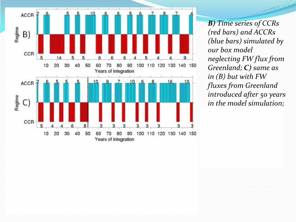
B) Time series of CCRs (red bars) and ACCRs (blue bars) simulated by our box model neglecting FW flux from Greenland; C) same as in (B) but with FW fluxes from Greenland introduced after 50 years in the model simulation; D) same as in (C) but with a doubling of FW fluxes from Greenland. Numbers by the bars indicate the regime duration in years.
B) Time series of CCRs (red bars) and ACCRs (blue bars) simulated by our box model neglecting FW flux from Greenland; C) same as in (B) but with FW fluxes from Greenland introduced after 50 years in the model simulation; D) same as in (C) but with a doubling of FW fluxes from Greenland. Numbers by the bars indicate the regime duration in years.
7 years 5 years 8 years 4 years
16 years !
5 years 9 years 5 years
8 years
GSA 1970s
GSA 1980s
GSA 1990s
CCR ACCR

8/6/2014 The 2014 OCB Summer Workshop 40
Concluding remarks:
Based on the analysis presented here we speculate that:
• Ocean-atmosphere heat fluxes in the GIN Sea vary with
circulation regimes and regulate interactions between the Arctic
Ocean and GIN Sea. Ocean to atmosphere heat fluxes are larger
during ACCRs (compared to CCRs) supporting cyclogenesis and
ultimately a regime shift to a CCR;
• The duration of ACCRs and CCRs in a changing climate will be
different from those in the 20st century; a new mode of variability
in the Arctic may consist of long-duration ACCRs, separated by
relatively short duration CCRs.
• The major cause of cessation of decadal variability is the
monotonically increasing FW flux anomaly from Greenland that
began in the mid 1990s, coincident with a shift to a positive AOO.
8/6/2014 The 2014 OCB Summer Workshop 41
Concluding remarks:
Based on the analysis presented here we speculate that:
• Ocean-atmosphere heat fluxes in the GIN Sea vary with
circulation regimes and regulate interactions between the Arctic
Ocean and GIN Sea. Ocean to atmosphere heat fluxes are larger
during ACCRs (compared to CCRs) supporting cyclogenesis and
ultimately a regime shift to a CCR;
• The duration of ACCRs and CCRs in a changing climate will be
different from those in the 20st century; a new mode of variability
in the Arctic may consist of long-duration ACCRs, separated by
relatively short duration CCRs.
• The major cause of cessation of decadal variability is the
monotonically increasing FW flux anomaly from Greenland that
began in the mid 1990s, coincident with a shift to a positive AOO.
1997 2001
Germe, A., M.-N. Houssais, C. Herbaut, and C. Cassou (2011), Greenland Sea sea ice variability over 1979–2007 and its link to the surface atmosphere, J. Geophys. Res., 116, C10034, doi:10.1029/2011JC006960.
Increase of sea ice coverage in the GIN Sea Less cyclonic acitivy Cooling climate And…
1970 1980 1990 2000 2010
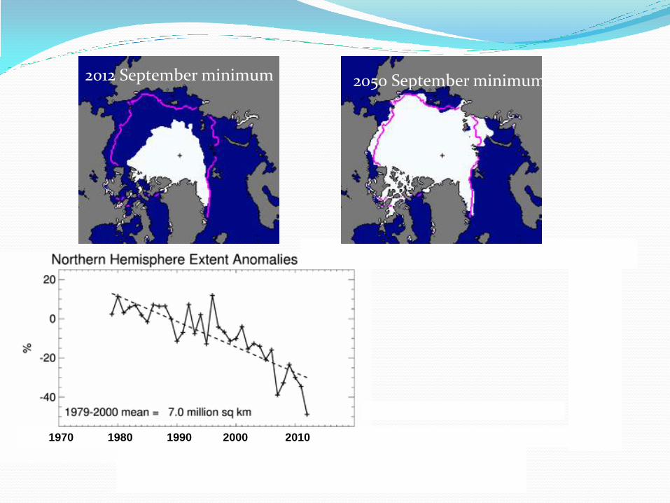
2012 September minimum 2050 September minimum
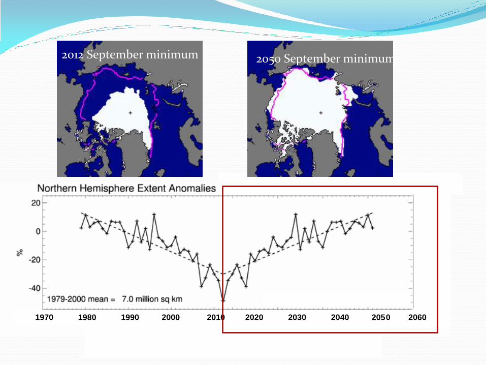
1970 1980 1990 2000 2010 2020 2030 2040 2050 2060
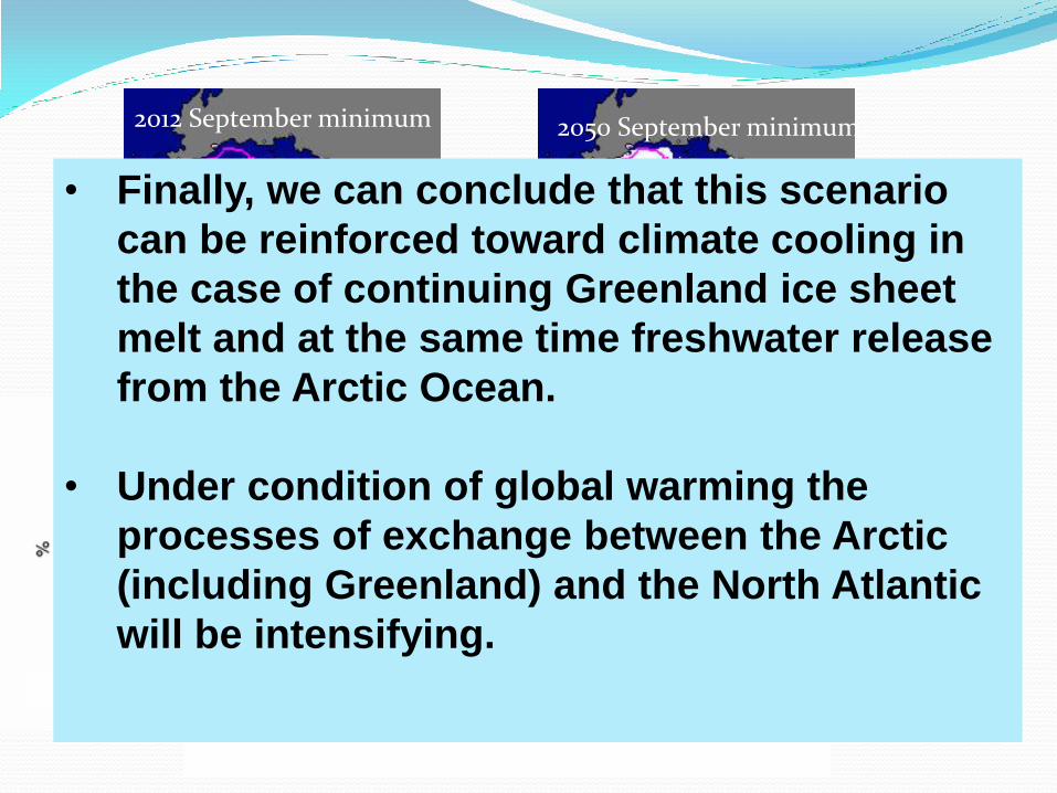
2012 September minimum 2050 September minimum
1970 1980 1990 2000 2010 2020 2030 2040 2050 2060
2012 September minimum 2050 September minimum
• Finally, we can conclude that this scenario
can be reinforced toward climate cooling in
the case of continuing Greenland ice sheet
melt and at the same time freshwater release
from the Arctic Ocean.
• Under condition of global warming the
processes of exchange between the Arctic
(including Greenland) and the North Atlantic
will be intensifying.