The 15 Percent Solution - Pacific Research

The 15 Percent Solution:Defining the Affordable Level of Government

Wayne Winegarden

BEYOND the NEW NORMALHow Much Should We Spend?

PART ONE

MAY 2018

Beyond the New Normal: Establishing a Pro-Growth Economic Policy EnvironmentHow Much Should We Spend?Defining the Affordable Level of Government

May 2018

Pacific Research Institute 101 Montgomery Street, Suite 1300San Francisco, CA 94104 Tel: 415-989-0833 Fax: 415-989-2411 www.pacificresearch.org

Download copies of this study at www.pacificresearch.org.

Nothing contained in this report is to be construed as necessarily reflecting the views of the Pacific Research Institute or as an attempt to thwart or aid the passage of any legislation.

©2018 Pacific Research Institute. All rights reserved. No part of this publication may be re-produced, stored in a retrieval system, or transmitted in any form or by any means, electronic, mechanical, photocopy, recording, or otherwise, without prior written consent of the publisher.

ContentsIntroduction ..........................................................................................................5

Government Spending from an Affordability Framework .................... 7

Defining an Affordable Federal Government .............................................9

The Implications from the Affordability Framework ............................13

Conclusion ........................................................................................................... 17

Appendix ..............................................................................................................18

Endnotes ............................................................................................................. 20

About the Author ..............................................................................................22

About PRI .............................................................................................................23

5The 15 Percent Solution: Defining the Affordable Level of Government

IntroductionWhen working properly, the public sector and the private sector have a beneficial relationship. A vibrant private economy relies on core government services to function efficiently, and the gov-ernment relies on a vibrant private economy to sufficiently fund those public services.

In practice, strains between the public and private sectors have emerged because the federal government has a spending problem. The manifestation of this problem is the excessive and profligate spending of the past half-century.

There are many ways to recognize the government’s spending problem, and Figure 1 presents two. Figure 1 compares total federal government outlays as a percentage of national income, to-tal federal government revenues as a percentage of national income, and the difference between these two trends (e.g. the annual deficit/surplus) between 1962 and 2016.1

One way to define the federal government’s spending problem is its inability to limit spending to the amount of money raised. Figure 1 illustrates that since 1962 total federal outlays exceeded total federal revenues, and particularly since the significant acceleration of outlays relative to national income began in the mid-1970s. Since 1975, when the significant acceleration of the spending problem became evident, outlays have exceeded revenues by 3.7 percentage points of national income annually.

Figure 1 Total Federal Government Revenues as a Percentage of National Income and Total Federal Outlays as a Percentage of National Income - 1962–2016

0.0%

5.0%

10.0%

15.0%

20.0%

25.0%

30.0%

35.0%

1962

19

64

1966

19

68

1970

19

72

1974

19

76

1978

19

80

1982

19

84

1986

19

88

1990

19

92

1994

19

96

1998

20

00

2002

20

04

2006

20

08

2010

20

12

2014

20

16

TOTAL OUTLAYS % NATIONAL INCOME AVERAGE TOTAL OUTLAYS % OF NATIONAL INCOME TOTAL REVENUES % NATIONAL INCOME AVERAGE TOTAL REVENUES % OF NATIONAL INCOME

Source: Office of Management and Budget

6 Beyond the New Normal: How Much Should We Spend?

The other way to recognize the government’s spending problem is to focus on the trend in total federal outlays as a percentage of national income. As Figure 1 illustrates, since 1975 total federal outlays have equaled 23.7 percent of national income. As of 2016 it was right around the 42-year average at 24.0 percent. This begs the question: is such an expenditure level affordable?

The answer to the affordability question depends on the definition of affordability, of course. One way to answer that question is to define affordability based on the historical revenue trends. Based on this defi-nition, relative to national income, the affordable lev-el of government is 20.0 percent of national income. This means that average annual expenditures need to be reduced by 3.7 percent.

Alternatively, affordability can be defined based on the government’s impact on the private economy. As illustrated in detail below, when government spend-ing reaches excessive levels, the beneficial relationship between the government and the private economy begins to break down. As the beneficial relationship breaks down, people pay the price in terms of lost opportunities, lost incomes, and lower overall living standards.

Due to this negative impact on the private economy from excessive government spending, this paper argues the appropriate definition of affordability is the level of government spending that maximizes the symbiotic relationship between the private economy and the public sector. All spending past this affordability threshold will, by definition, detract from economic growth rath-er than contribute to economic growth.

If a growth-maximizing affordability level exists, then it must be the case that restricting expen-ditures to this level will maximize fiscal policy’s positive impact on the economy’s growth rate. Further, since there is no reason to believe that the historical experience is reasonably close to this definition of an affordable level of government, there is an opportunity to accelerate the econ-omy’s average growth rate by conforming federal expenditures to the growth maximizing rate.

The evidence presented below indicates that the current level of federal government expenditures significantly exceeds this growth maximizing definition of the affordable level of government spending – by around 8 to 10 percentage points of national income. In terms of the 2016 federal expenditures, the growth maximizing rate of federal expenditures would have been between $2.2 trillion and $2.6 trillion based on the calculations below, rather than actual expenditures of $3.9 trillion. Put differently, the estimates below imply that total federal expenditures are 50 percent to 71 percent too large.

The purpose of this paper is to set out the logic of the affordability constraint on government spending, provide estimates of this affordability threshold in practice, and discuss the pragmatic implications of fiscal policy from an affordability perspective.

The other way to recognize the government’s spending problem is to focus on the trend in total federal outlays as a percentage of national income.


Government Spending from an Affordability Framework The government faces an affordability constraint because the economic principle of diminishing value – the benefits people receive from consuming any good or service declines the more of that good consumed – applies equally to public goods and services as it does to private goods and services. Applied to the public sector, initially there are large positive benefits to the economy from government spending; but as government spending grows, the positive benefits from that spending to the economy declines. Ultimately, there is a point where additional government spending does not provide any more benefits – the expenditures have become a net negative for the economy.

In Beyond the New Normal: Accounting for Government, we illustrated this point using the example of a firehouse. Establishing a firehouse in a town without one provides tremendous value. Now, trained professionals can fight fires and reduce the dangers and damage created by fires. If the town is large, a second firehouse will also provide tremendous value, although slightly less value than the first. There comes a point where funding an additional firehouse does not sufficiently improve the town’s safety, relative to the cost of establishing the firehouse. Paying for firehouses beyond this level detracts from the town’s welfare.

Several analyses have also recognized that government spending exhibits diminishing returns. For example, Mitchell (2005) noted that

…almost every economist would agree that there are circumstances in which lower levels of government spending would enhance economic growth and other circumstances in which higher levels of government spending would be desirable. If government spending is zero, presumably there will be very little economic growth because enforcing contracts, protecting property, and developing an in-frastructure would be very difficult if there were no government at all. In other words, some government spending is necessary for the successful operation of the rule of law.2

Larson (2007) refers to this relationship as the Rahn Curve3 because

this curve was popularized by Richard Rahn, the former chief economist of the U.S. Chamber of Commerce and defines a largely negative relationship between economic growth and the burden of government spending…the Rahn Curve’s message is that growth is maximized when government spending is modest – and presumably allocated for core public goods like protection of life, liberty and property – but that growth deteriorates when government expands beyond this limited level.

The growth-maximizing point on the Rahn Curve is the subject of consider-able research. Academic experts generally conclude that this point is somewhere


between 15 percent of GDP and 25 percent of GDP [17 percent to 29 percent of national income], though it is likely that these estimates are too high since the statistical studies are constrained by a lack of data for countries with limited governments.4

According to Rahn (2016) the results, show “that there was a negative relationship [from gov-ernment spending on economic growth] once government exceeded roughly a quarter of GDP.”5 Research by “…Gerald Scully of the University of Texas, Robert Barro of Harvard University, independently using much more data and a more sophisticated analysis, found the same neg-ative relationship between government growth as a share of GDP and economic growth.”6 In an update to this work, Scully (2006), estimated that the growth maximizing federal, state, and local tax burden is 23 percent of GDP, or 27 percent of national income.7 In another anal-ysis, Niskanen (2003) found that the optimal size of the federal government, excluding defense spending, is around 10 percent of GDP, or 12 percent of national income.8

Advocates for greater government spending, particularly stimulative spending, fail to consis-tently apply the concept of diminishing returns to public goods. Instead, these advocates will argue that due to the existence of the “economic multiplier”, additional government spending increases overall aggregate demand. Thus, these theorists will argue that government spend-

ing has a positive impact on the economy, regardless of how much the government is already spending.

Such a position is inconsistent with the fundamental tenet of diminishing value, however. Viewing government spending from an affordability framework simply recognizes that expenditures on public goods are no different from expenditures on private economic goods. The addition-al value citizens receive from public goods and services will be initially high but de-cline as the government provides more and more of these goods and services.9

The implication is that when government expenditures are below the efficient level,

increasing government spending contributes to overall economic growth; but, when expenditures are above the efficient level, increasing government spending detracts from economic growth. Thus, there is an optimal level of government spending, what we term the affordable level of gov-ernment spending. At this affordable level, the federal government’s expenditures will be having the largest positive impact on the economy’s rate of growth.

A problem arises, however, because unlike transactions in purely private markets, government spending does not benefit from an automatic correction mechanism to ensure that the affordable amount of government expenditures prevail. In private markets, consumers have a sense of the goods and services they want to purchase; the value they will receive from different combinations

Viewing government spending from an affordability framework simply recognizes that expenditures on public goods are no different from expenditures on private economic goods.


of these goods and services; and, will directly bear the costs of paying for these goods and ser-vices. Suppliers, on the other hand, know the costs required to provide these goods and services and reap the rewards from selling them (e.g. earn a profit). Mistakes, of course, happen.

Sometimes consumers regret their purchases, or suppliers sell goods that too few consumers want. These mistakes do not persist, however. Suppliers who consistently sell goods that con-sumers do not want will go out of business. Consumers who regret a past purchase will, pre-sumably, change their purchasing habits in the future. Through this dynamic process, private markets roughly provide people with the types and amounts of goods and services that maximize value given their income constraints.

When it comes to government expenditures, the people paying for the service differ from the people consuming the service. Further, the government providers of the service do not receive any product feedback. Therefore, there is no automatic mechanism for the consumers of the public goods and services to tell the government how much value the public goods are providing them. Nor, is there a direct way for the people funding the public goods and services (who may differ from the people consuming those services) to tell the government how much they value the level and composition of the public goods and services provided.

Since there is no automatic mechanism to optimize the size of the federal budget, it is import-ant to establish budgetary rules that constrain spending to an affordable share of the economy. Establishing a budget constraint that is consistent with the growth maximizing size of the gov-ernment places restrictions on the federal government’s expenditures in the same way that the workers’ incomes or businesses’ revenues place restrictions on their expenditures. In short, im-posing a hard budget constraint on federal expenditures forces the federal government to make the necessary budgetary trade-offs.

These trade-offs are no different than the trade-offs that every other organization or family must make on a regular basis. In short, the government is not exempt from another fundamental premise of economics – that there are scarce resources but unlimited wants. It is not enough to say that a potential government program has value. The value created by a government program must be evaluated against the benefits gained if those resources were not extracted from the private economy in the first place. Only government programs that pass this test should be con-sidered.

Defining an Affordable Federal GovernmentThe discussion above illustrates that government spending is not detrimental to growth per se, but additional government spending (what economists refer to as marginal increases in spend-ing) is currently detrimental to economic growth because the government is already spending too much. Put differently, the current size of the federal government is past the optimal growth portion of the Rahn Curve.


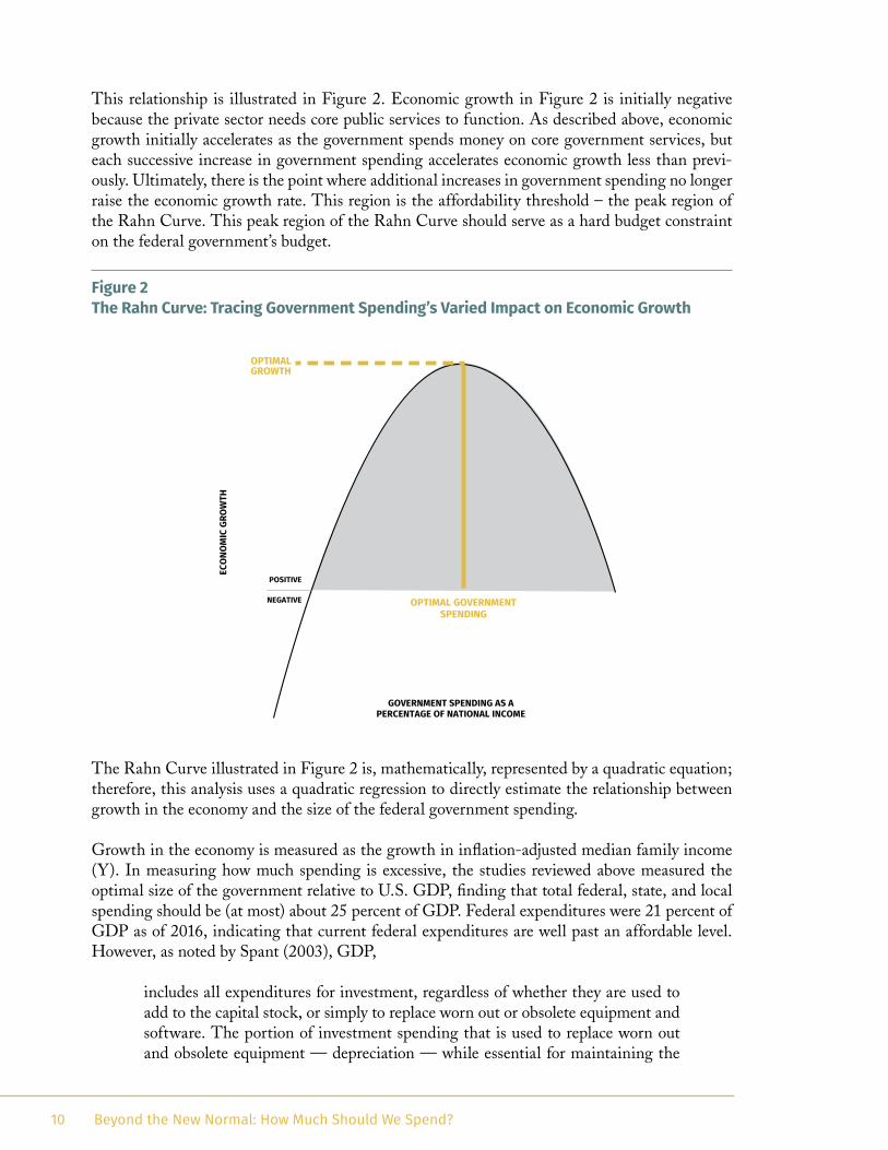
This relationship is illustrated in Figure 2. Economic growth in Figure 2 is initially negative because the private sector needs core public services to function. As described above, economic growth initially accelerates as the government spends money on core government services, but each successive increase in government spending accelerates economic growth less than previ-ously. Ultimately, there is the point where additional increases in government spending no longer raise the economic growth rate. This region is the affordability threshold – the peak region of the Rahn Curve. This peak region of the Rahn Curve should serve as a hard budget constraint on the federal government’s budget.

Figure 2 The Rahn Curve: Tracing Government Spending’s Varied Impact on Economic Growth

The Rahn Curve illustrated in Figure 2 is, mathematically, represented by a quadratic equation; therefore, this analysis uses a quadratic regression to directly estimate the relationship between growth in the economy and the size of the federal government spending.

Growth in the economy is measured as the growth in inflation-adjusted median family income (Y). In measuring how much spending is excessive, the studies reviewed above measured the optimal size of the government relative to U.S. GDP, finding that total federal, state, and local spending should be (at most) about 25 percent of GDP. Federal expenditures were 21 percent of GDP as of 2016, indicating that current federal expenditures are well past an affordable level. However, as noted by Spant (2003), GDP,

includes all expenditures for investment, regardless of whether they are used to add to the capital stock, or simply to replace worn out or obsolete equipment and software. The portion of investment spending that is used to replace worn out and obsolete equipment — depreciation — while essential for maintaining the

OPTIMALGROWTH

OPTIMAL GOVERNMENTSPENDING

POSITIVE

NEGATIVE

ECO

NOM

IC G

ROW

TH

GOVERNMENT SPENDING AS APERCENTAGE OF NATIONAL INCOME


level of output, does not increase the economy’s capacities in any way. If GDP were to grow simply as a result of the fact that more money was being spent to maintain the capital stock because of increased depreciation, it would not mean that anyone had been made better off. There would be no more resources avail-able for consumption. Nor would there be any more output available in future periods, because the size of the capital stock would not have increased.

In such a scenario, since equipment is wearing out more quickly, it is necessary to run harder just to stay in the same place. The economy must devote more re-sources every year to replace worn out and obsolete equipment, just to keep the capital stock intact. The additional resources used to replace this equipment are recorded in the national accounts, but it does not imply that anyone is better off.10

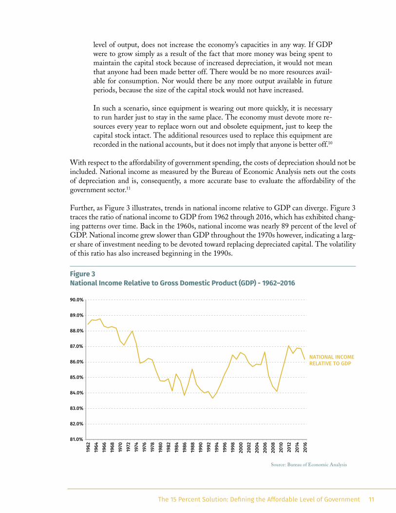
With respect to the affordability of government spending, the costs of depreciation should not be included. National income as measured by the Bureau of Economic Analysis nets out the costs of depreciation and is, consequently, a more accurate base to evaluate the affordability of the government sector.11

Further, as Figure 3 illustrates, trends in national income relative to GDP can diverge. Figure 3 traces the ratio of national income to GDP from 1962 through 2016, which has exhibited chang-ing patterns over time. Back in the 1960s, national income was nearly 89 percent of the level of GDP. National income grew slower than GDP throughout the 1970s however, indicating a larg-er share of investment needing to be devoted toward replacing depreciated capital. The volatility of this ratio has also increased beginning in the 1990s.

Figure 3 National Income Relative to Gross Domestic Product (GDP) - 1962–2016

81.0%

82.0%

83.0%

84.0%

85.0%

86.0%

87.0%

88.0%

89.0%

90.0%

1962

19

64

1966

19

68

1970

19

72

1974

19

76

1978

19

80

1982

19

84

1986

19

88

1990

19

92

1994

19

96

1998

20

00

2002

20

04

2006

20

08

2010

20

12

2014

20

16

National Income Relative to GDP

NATIONAL INCOME RELATIVE TO GDP

Source: Bureau of Economic Analysis


These changing patterns between national income and GDP indicate that there may be mean-ingful differences if the affordability of government expenditures is estimated based on GDP rather than national income, which is why the more relevant measure of national income is used as the basis to judge the size of the federal government. Specifically, the size of the federal gov-ernment is measured as total federal outlays as a share of national income (O), and total federal outlays as a share of national income squared (O2), in order to account for the possibility that there is an optimal level of government spending.

Of course, there are many other economic trends that can impact the growth in inflation-adjust-ed median family income. To account for these trends, the regression includes two broad macro-economic variables: the difference in logs in inflation-adjusted GDP per capita (GDP) and the average unemployment rate for the year (Un).

With respect to the expected impacts on the growth in inflation-adjusted me-dian family income, total federal outlays should initially have a positive impact on the economy, which indicates that the total federal outlays as a share of nation-al income should be positively related to median family income. Since the positive benefits of government expenditures on inflation-adjusted median family income should decline as its size increases, total federal outlays as a share of national in-come squared should be negatively related to median family income. These are the main relationships the analysis estimates.

As for the other factors that will impact median family income, the change in inflation-adjusted GDP per capita is ex-pected to be positively related to increases in inflation-adjusted median family in-come (as the economy is stronger, fam-ily incomes should be rising faster); and

the unemployment rate should be negatively related to inflation-adjusted median family income growth (when there are excessive amounts of workers looking for employment relative to the available jobs, family incomes should be declining). The details of the alternative regressions are presented in the Appendix. Summarizing the results, the variables had the expected signs, and all were significantly related to growth in median family incomes, except the unemployment rate.

Most important for this analysis, the analyses indicated that growth in median family income is optimized when federal government expenditures are between 14 percent and 16 percent of national income. Running the same analyses for state and local government spending and com-bining the results, median family income is the fastest when total federal, state, and local gov-ernment spending is between 23 percent and 27 percent of national income.12 These values are consistent with Rahn’s and Scully’s estimates cited previously.

With respect to the expected impacts on the growth in inflation-adjusted median family income, total federal outlays should initially have a positive impact on the economy, which indicates that the total federal outlays as a share of national income should be positively related to median family income.


The Implications from the Affordability FrameworkImportant implications arise once the concept that government expenditures exhibit diminishing additional value is recognized. The first implication is that total government expenditures should be subject to a hard budget cap, or an aggregate budget constraint. The aggregate budget con-straint reflects the marginal value created by a dollar spent by the public sector compared to the marginal value created by the dollar had it remained in the private sector. As estimated above and based on the growth-maximizing definition of affordability, the aggregate budget constraint at the federal level should be between 14 percent and 16 percent of national income.

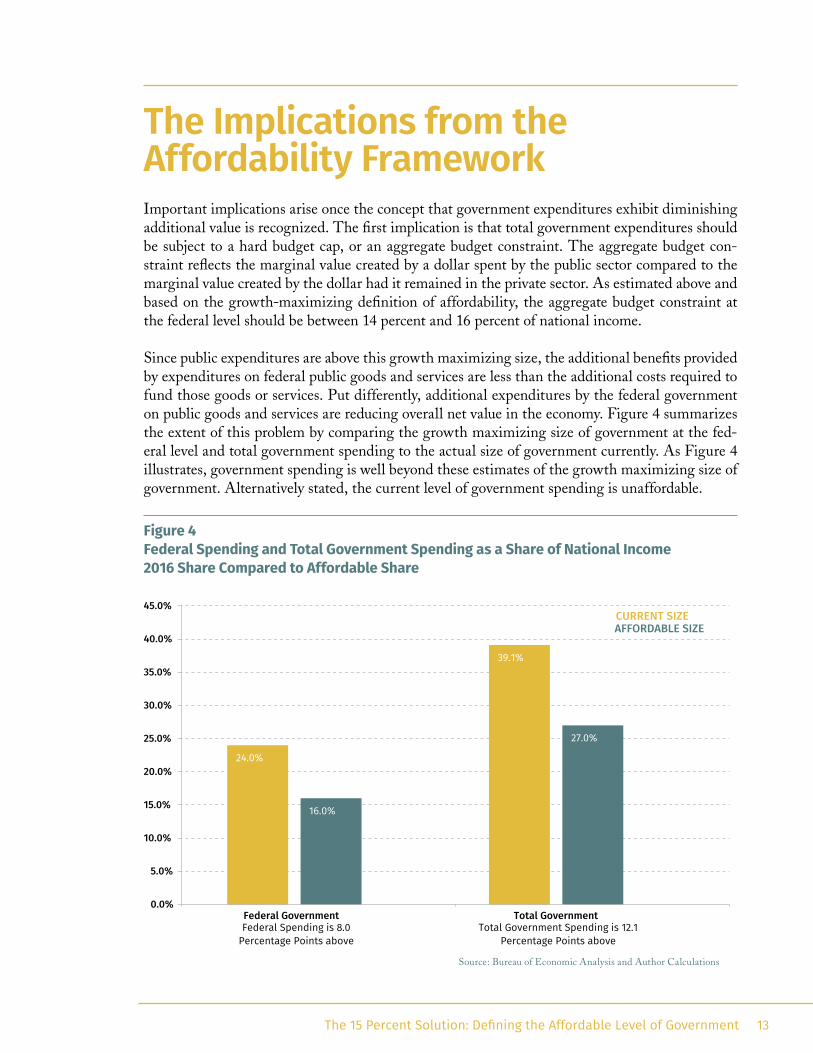
Since public expenditures are above this growth maximizing size, the additional benefits provided by expenditures on federal public goods and services are less than the additional costs required to fund those goods or services. Put differently, additional expenditures by the federal government on public goods and services are reducing overall net value in the economy. Figure 4 summarizes the extent of this problem by comparing the growth maximizing size of government at the fed-eral level and total government spending to the actual size of government currently. As Figure 4 illustrates, government spending is well beyond these estimates of the growth maximizing size of government. Alternatively stated, the current level of government spending is unaffordable.

Figure 4 Federal Spending and Total Government Spending as a Share of National Income 2016 Share Compared to Affordable Share

24.0%

39.1%

16.0%

27.0%

0.0%

5.0%

10.0%

15.0%

20.0%

25.0%

30.0%

35.0%

40.0%

45.0% CURRENT SIZE AFFORDABLE SIZE

Federal Government Total Government Federal Spending is 8.0

Percentage Points aboveAffordability Range

Total Government Spending is 12.1Percentage Points above

Affordability RangeSource: Bureau of Economic Analysis and Author Calculations


Focusing on the federal government expenditures, the topic of this analysis, the federal govern-ment has been providing unaffordable levels of government expenditures for at least the past 50 years, which is why empirical studies that examine the relationship between government spend-ing and economic growth typically find a negative relationship.13 Further, the cost in terms of lost growth and lost income are significant. Had government spending remained at the affordable level, the median family income could be 34 percent higher as of 2016 than it was – $97,185 rather than the actual value of $72,707.

Bringing expenditures in line with current reve-nue trends requires steep reductions in the total expenditures relative to national income. To min-imize the transition costs, a gradualist approach is warranted. This approach should cap the growth in inflation adjusted spending to less than the aver-age growth in inflation adjusted national income. Since federal expenditures would now be growing slower than the growth in the private sector’s abil-ity to fund these expenditures, over time, such a growth cap would reduce federal spending to the affordability level that, as estimated here, should be between 14 percent and 16 percent of national income.

If the goal is to structurally balance the federal budget within a decade (e.g. bring spending to 20 percent of national income within 10-years), then the growth of federal government spending would need to be restricted to 2 percentage points below the average growth in inflation-adjusted national income. Assuming a 2 percent inflation rate, this cap implies annual growth in the fed-eral budget of 3 percent per year. Further, at this pace, federal government expenditures would reach the top-end of the affordability level (16 percent of national income) within two decades – see Figure 5. Importantly, these estimates do not account for the dynamic growth impacts. Since government expenditures would become more affordable every year, economic growth would accelerate relative to its historic growth path. Thus, these timeframes should be viewed as conservative estimates. Once federal expenditures have reached the pre-defined affordability level, the growth rule constraining federal expenditures should be amended to equal the average growth in national income.

Bringing expenditures in line with current revenue trends requires steep reductions in the total expenditures relative to national income.


Figure 5 Projected Federal Revenues as a Percentage of National Income Constrained to a National Income Minus 2-percent Rule

0.0%

5.0%

10.0%

15.0%

20.0%

25.0%

30.0%

2017

2018

2019

2020

2021

2022

2023

2024

2025

2026

2027

2028

2029

2030

2031

2032

2033

2034

2035

2036

2037

2038

2039

SPENDING % NI

AVERAGE REVENUES % NI

TOP-END AFFORDABILITY RATE

Source: Author Calculations

Establishing the affordable level of government is only the beginning of the process, however. The composition of government spending matters because public goods and services are not a homogenous product. Instead, what we term as “public goods” are an amalgamation of very dif-ferent types of goods and services. Further, there is no reason to believe that the net value added gained from additional expenditures on one type of public good (e.g. defense expenditures) will be similar to the net value added gained from additional expenditures on another type of public good (e.g. education expenditures). Therefore, a second implication is that how expenditures are allocated across programs is critically important. There are, consequently, compositional effi-ciencies in the provision of public goods and services that must be addressed within the aggregate budget constraint.

Government expenditures create value when they fund public goods and services whose addi-tional value of that specific program exceeds the value of those resources had they remained in the private sector (they are positive NPV projects). The value gained from additional defense expenditures may be less than the additional costs necessary to fund those services, while the net value added gained from additional education expenditures may exceed those costs; or vice versa. An effective budget cap implies that any necessary increase in expenditures for one programmat-ic area must be prioritized relative to all other potential programs.

Therefore, it is possible (probable) that within the aggregate budget constraint, a reorganization of how federal government expenditures are spent is warranted – a reprioritization of federal ex-penditures will increase the additional value enabled by the federal government. Pragmatically, these compositional considerations have important consequences. Even as the current level of


federal government expenditures far exceeds an affordable size of government, it is not enough to simply randomly control spending. The composition of federal expenditures matters. In part, the purpose of the aggregate budget cap is to force legislators to establish spending priorities that, in the ideal, would reflect the efficient composition of public goods and services.

Identifying areas of waste, duplication, and redundancies across the government are also import-ant as such expenditures, by definition, are negative NPV expenditures. Due to the enormity of this topic, the important issue of creating a more effective composition of government spending is only being raised in this paper; it will be analyzed in much greater detail in follow-on analyses in the Beyond the New Normal series.

A third implication involves the futility of stimulus spending given the current size of the federal govern-ment. For example, President Obama and Congress implemented the American Recovery and Reinvest-ment Act (ARRA) in 2009 as a fiscal stimulus that was supposed to accelerate the economic recovery from the Great Recession. Despite its stated inten-tions, ARRA was destined to detract from econom-ic growth because the level of federal government spending was already above the affordable level. Sim-ply put, the value of the public goods provided by the ARRA programs was far less than the value of those resources had they remained in the private sector – essentially these programs had a negative net present value (NPV).

A fourth implication involves the timing of expen-ditures on positive NPV projects. Recognizing that government expenditures can, but do not necessari-ly, improve economic growth fundamentally changes

how the federal government should approach its spending – particularly so-called stimulative government expenditures. Specifically, if an affordable positive NPV project exists, should the government provide these public goods and services immediately, or wait until there is a reces-sion to stimulate the economy? After all, forgoing these expenditures means denying citizens the benefits from a welfare enhancing public good or service. But, if government programs that can improve citizens’ welfare should be undertaken regardless of whether the economy is in recession, or a robust expansion, then the implication is that the federal government should not attempt to implement active counter-cyclical policies, but instead focus on ensuring that the pub-lic sector is meeting the positive NPV benchmarks as efficiently as possible. Therefore, once the affordability framework is taken seriously, it becomes clear that the federal government should not be conducting stimulative fiscal policy regardless of whether current expenditures exceed the affordability threshold. Either government programs benefit the economy and should be pur-sued, or they impose a net cost on the economy and should be avoided. The stage of the business cycle is not the driving factor.

Identifying areas of waste, duplication, and redundancies across the government are also important as such expenditures, by definition, are negative NPV expenditures.


ConclusionAs the previous studies in the Pacific Research Institute’s Beyond the New Normal research pro-gram have noted, federal fiscal policy must be improved before the U.S. economy will fully regain its past robust growth performance. With respect to overall spending, for too long the federal government has acted as if resources are not scarce. And, as a result, the unaffordable federal government expenditures are obstructing economic growth instead of promoting over-all economic welfare. The costs in terms of lost wealth and lost opportunity are both large and growing. Consequently, the benefits from establishing an affordable federal government cannot be understated.

Past studies that have examined the issue, as well as the estimates provided in this paper, indi-cate that an affordable size of the federal government is between 14 percent and 16 percent of National Income – 8 to 10 percentage points below the 2016 level of 24 percent. In response, an aggregate expenditure cap should be imposed on the federal government. If expenditure growth is restricted to 2 percentage points below the average growth in national income, then the budget can be balanced within a decade, and federal expenditures will be affordable once again within two decades.

While this paper described the affordability framework that should guide the federal govern-ment’s budget process, it has not addressed the fundamental issue of how. Just as a household living within its means is insolvent if it spends all its money at the racetrack, the benefits from imposing an affordable budget will be lost without also establishing an effective composition of federal spending. These vitally important questions will be addressed in a series of follow-up analyses. Taken together, these studies provide a comprehensive framework to help create a more affordable and more effective federal budget.


AppendixThe quadratic regression analysis for the federal expenditure analysis estimated the following equation:

A1: LN (Yt – Yt-1) = b1 * O + b2 * O2 + b3* LN (GDPt – GDPt-1) + b4 * Un; where:

Y: Inflation-adjusted median family income; O: Total federal outlays as a share of national income; O2: Total federal outlays as a share of national income squared;GDP: Inflation-adjusted GDP per capita;Un: Average unemployment rate for the year.

Equation A1 was estimated both with and without the control variables GDP and Un to test for the consistency of the coefficients of interest, O and O2. The results are presented in Table A-1. As Table A-1 illustrates, the variables have the expected impacts on inflation-adjusted median family income and were significant at the 5-percent level, except for the unemployment rate variable.

Table A-1 Regression Coefficients Dependent Variable: Log Differences in Inflation-adjusted Median Family Income

ESTIMATED COEFFICIENTS

Federal Expenditures percent NI 0.54 0.28

P-value* 0.00 0.01

Federal Expenditures percent NI ^2 (2.15) (0.92)

P-value 0.00 0.04

Log Differences Inflation-adjusted GDP/Cap 0.69

P-value* 0.00

Unemployment Rate (0.28)

P-value 0.22

Adj. R-Square 0.33 0.60

Durbin-Watson Statistic 1.83

* Significant at the 1-percent level.

Figure A-1 presents the actual change in inflation-adjusted median family income to the change in inflation-adjusted median family that would be estimated by equation A1 using both the full data sample, and two-thirds of the data sample (in order to see how the estimates would predict). Figure A-1 illustrates that the model closely predicts the change in inflation-adjusted median family income using both the full data sample and two-thirds of the data sample.


Figure A-1 Actual Inflation-adjusted Median Family Income Compared to Predicted Inflation-adjusted Median Family Income - 1962–2016

-8.0%

-6.0%

-4.0%

-2.0%

0.0%

2.0%

4.0%

6.0%

8.0% 19

54

1956

19

58

1960

19

62

1964

19

66

1968

19

70

1972

19

74

1976

19

78

1980

19

82

1984

19

86

1988

19

90

1992

19

94

1996

19

98

2000

20

02

2004

20

06

2008

20

10

2012

20

14

2016

Predicted (full sample) % Change Real Family Income Predicted (2/3 sample)


Endnotes1 Throughout this paper, National Income is used as the measure of the private economy rather

than GDP to adjust for depreciation.

2 Mitchell D.J. (2005) “The Impact of Government Spending on Economic Growth” Heritage Foundation Backgrounder, No. 1831, March 31.

3 The Rahn Curve is predicated on the same logic as the Laffer Curve.

4 Larson S.R. (2007) “The Economic Case for Limited Government” Prosperitas Vol. 7 Issue 3, April; http://archive.freedomandprosperity.org/Papers/rahncurve/rahncurve.pdf.

5 Rahn R. (2016) “The optimum size of governmental units” Cayman Financial Review, No-vember 1; http://www.caymanfinancialreview.com/2016/11/01/the-optimum-size-of-gov-ernmental-units/.

6 Rahn R. (2016) “The optimum size of governmental units” Cayman Financial Review, No-vember 1; http://www.caymanfinancialreview.com/2016/11/01/the-optimum-size-of-gov-ernmental-units/.

7 Scully G.W. (2006) “Taxes and Economic Growth” National Center for Policy Analysis, Report No. 292 November.

8 Niskanen W.A. (2003) “The economic burden of taxation” Proceedings: Federal Reserve Bank of Dallas, October; https://econpapers.repec.org/article/fipfeddpr/y_3a2003_3ai_3aoc-t_3ap_3a93-98.htm.

9 For an in-depth discussion of this issue see: Winegarden W. and Chura N. (2017) “Be-yond the New Normal: Accounting for Government” Pacific Research Institute, February 3; https://www.pacificresearch.org/beyond-the-new-normal-part-2-accounting-for-govern-ment/.

10 Spant R. (2003) “Why Net Domestic Product Should Replace Gross Domestic Product as a Measure of Economic Growth” International Productivity Monitor, No. 7, Fall; http://www.csls.ca/ipm/7/spant-e.pdf.

11 For the relation between GDP and National Income see the Bureau of Economic Anal-ysis Table 1.7.5; https://www.bea.gov/iTable/iTable.cfm?reqid=19&step=2#reqid=19&-step=3&isuri=1&1921=survey&1903=43.

http://archive.freedomandprosperity.org/Papers/rahncurve/rahncurve.pdf

http://www.caymanfinancialreview.com/2016/11/01/the-optimum-size-of-governmental-units/




https://econpapers.repec.org/article/fipfeddpr/y_3a2003_3ai_3aoct_3ap_3a93-98.htm

https://econpapers.repec.org/article/fipfeddpr/y_3a2003_3ai_3aoct_3ap_3a93-98.htm

https://www.pacificresearch.org/beyond-the-new-normal-part-2-accounting-for-government/

https://www.pacificresearch.org/beyond-the-new-normal-part-2-accounting-for-government/

http://www.csls.ca/ipm/7/spant-e.pdf

http://www.csls.ca/ipm/7/spant-e.pdf


12 A regression analysis that used total federal, state, and local revenues as the dependent vari-able was also performed. The coefficients signs and significance levels were similar to the analyses run individually. This analysis indicated that the optimal affordability range for total federal, state, and local expenditures was 20 percent to 23 percent of National Income.

13 For a review of the academic literature linking higher taxes to less economic growth see: Mc-Bride W. (2012) “What Is the Evidence on Taxes and Growth?” Tax Foundation, December 18, No. 207.


About the AuthorWayne H. Winegarden, Ph.D. is a Senior Fellow in Business and Economics, Pacific Research Institute, as well as the Principal of Capitol Economic Advisors and a Contributing Editor for EconoSTATS.

Dr. Winegarden has 20 years of business, economic, and policy experience with an expertise in applying quantitative and macroeconomic analyses to create greater insights on corporate strat-egy, public policy, and strategic planning. He advises clients on the economic, business, and in-vestment implications from changes in broader macroeconomic trends and government policies. Clients have included Fortune 500 companies, financial organizations, small businesses, state legislative leaders, political candidates and trade associations.

Dr. Winegarden’s columns have been published in the Wall Street Journal, Chicago Tribune, In-vestor’s Business Daily, Forbes.com, and Townhall.com. He was previously economics faculty at Marymount University, has testified before the U.S. Congress, has been interviewed and quoted in such media as CNN and Bloomberg Radio, and is asked to present his research findings at policy conferences and meetings. Previously, Dr. Winegarden worked as a business economist in Hong Kong and New York City; and a policy economist for policy and trade associations in Washington D.C. Dr. Winegarden received his Ph.D. in Economics from George Mason Uni-versity.


About PRIThe Pacific Research Institute (PRI) champions freedom, opportunity, and personal responsibil-ity by advancing free-market policy solutions. It provides practical solutions for the policy issues that impact the daily lives of all Americans, and demonstrates why the free market is more effec-tive than the government at providing the important results we all seek: good schools, quality health care, a clean environment, and a robust economy.

Founded in 1979 and based in San Francisco, PRI is a non-profit, non-partisan organization supported by private contributions. Its activities include publications, public events, media com-mentary, community leadership, legislative testimony, and academic outreach.

Center for Business and EconomicsPRI shows how the entrepreneurial spirit—the engine of economic growth and opportunity—is stifled by onerous taxes, regulations, and lawsuits. It advances policy reforms that promote a ro-bust economy, consumer choice, and innovation.

Center for Education PRI works to restore to all parents the basic right to choose the best educational opportunities for their children. Through research and grassroots outreach, PRI promotes parental choice in education, high academic standards, teacher quality, charter schools, and school-finance reform.

Center for the EnvironmentPRI reveals the dramatic and long-term trend toward a cleaner, healthier environment. It also examines and promotes the essential ingredients for abundant resources and environmental qual-ity: property rights, markets, local action, and private initiative.

Center for Health CarePRI demonstrates why a single-payer Canadian model would be detrimental to the health care of all Americans. It proposes market-based reforms that would improve affordability, access, quality, and consumer choice.

Center for California ReformThe Center for California Reform seeks to reinvigorate California’s entrepreneurial self-reliant traditions. It champions solutions in education, business, and the environment that work to ad-vance prosperity and opportunity for all the state’s residents.


www.pacificresearch.org

SAN FRANCISCO HEADQUARTERS101 Montgomery Street, Suite 1300San Francisco, CA 94104Tel 415-989-0833Fax 415-989-2411

SACRAMENTO OFFICE2110 K Street, Suite 28Sacramento, CA 95816Tel 916-389-9774

PASADENA OFFICE680 E. Colorado Blvd.Pasadena, CA 91107Tel 626-714-7572

Connect with Us

facebook.com/pacificresearchinstitute

@pacificresearch

youtube.com/pacificresearch1

www.linkedin.com/company/ pacific-research-institute

Documents

The 15 Percent Solution - Pacific Research