the Klein Gordon equation at least, both answers can be determined from considerations of groupvelocities.

§1.4. Fourier synthesis and rectilinear propagation.

For equations with constant coe!cients, solutions of the initial value problem are expressed asFourier integrals. Injecting short wavelength initial data and performing an asymptotic analysisyields the approximations of geometric optics. This is how such approximations were first justifiedin the nineteenth century. It is also the motivating example for the more general theory. The shortwavelength approximations explain the rectilinear propagation of waves in homogeneous media.This is the first of the three basic physical laws of geometric optics. It explains, among otherthings, the formation of shadows. The short wavelength solutions are also the building blocks inthe analysis of the laws of reflection and refraction.

Consider the initial value problem

u := utt !"u :=!2u

!t2!

d!

j=1

!2u

!x2j

= 0 , u(0, x) = f , ut(0, x) = g . (1.4.1)

Fourier transformation with respect to the x variables yields

!2t u(t, ") + |"|2 u(t, ") = 0 , u(0, ") = f , !tu(0, ") = g .

Solve the ordinary di#erential equations in t to find

u(t, ") = f(") cos t|"| + g(")sin t|"||"|

.

Write

cos t|"| =eit|!| + e!t|!|

2, sin t|"| =

eit|!| ! e!t|!|

2i,

to findu(t, ") = a+(") ei(x!!t|!|) ! a!(") ei(x!+t|!|) , (1.4.2)

with,

2 a+ := f +g

i|"|, 2 a! := f !

g

i|"|. (1.4.3)

The right hand side of (1.4.2) is an expression in terms of the plane waves ei(x!"t|!|) with amplitudesa±(") and dispersion relations # = "|"|. The group velocities associated to a± are

v = !#!# = !#!("|"|) = ±"

|"|.

The solution is the sum of two terms,

u"±(t, x) :=

1

(2$)d/2

"a±(") ei(x!"t|!|) d" .

Using F#!u/!xj

$= i"j u, and Parseval’s Theorem shows that the conserved energy for the wave

equation is equal to

1

2

"|ut(t, x)|2 + |#xu(t, x)|2 dx =

"|"|2

#|a+(")|2 + |a!(")|2

$d" .

17

There are conservations of all orders. Each of the following quantities is independent of time,

1

2$#t,xu(t)$2

Hs(Rd) =

"%"&2s |"|2

#|a+(")|2 + |a!(")|2

$d" .

Consider initial data a wave packet with wavelength of order % and phase equal to x1/%,

u"(0, x) = &(x) eix1/" , u"t(0, x) = 0 , & ' (sH

s(Rd) . (1.4.4)

The choice ut = 0 postpones dealing with the factor 1/|"| in (1.4.3). The initial value is an envelopeor profile & multiplied by a rapidly oscillating exponential.

Applying (1.4.3) with g = 0 and with

f(") = u(0, ") = F#&(x) eix1/"

$= &(" ! e1/%) ,

yields u = u+ + u! with,

u"±(t, x) :=

1

2

1

(2$)d/2

"&(" ! e1/%) ei(x!"t|!|) d" .

Analyse u"+. The other term is analogous. For ease of reading, the subscript plus is omitted.

Introduce' := " ! e1/%, " = e1 + %',

to find,

u"(t, x) =1

2

1

(2$)d/2

"&(') eix(e1+"#)/" e!it|e1+"#|/" d' . (1.4.5)

The approximation of geometric optics comes from injecting the first order Taylor approximation,

%%e1 + %'%% ) 1 + %'1 ,

yielding,

u"approx :=

1

2

1

(2$)d/2

"&(') eix(e1+"#)/" e!it(1+"#1)/" d' .

Collecting the rapidly oscillating terms ei(x1!t)/" which do not depend on ' gives,

uapprox = ei(x1!t)/" a(t, x), a(t, x) :=1

2

1

(2$)d/2

"&(') ei(x#!t#1) d' . (1.4.6)

Write x ! t'1 = (x ! te1).' to find,

a(t, x) =1

2

1

(2$)d/2

"&(') ei(x!te1)# d' =

1

2&(x ! te1) .

The approximation is a wave translating rigidly with velocity equal to e1. The waveform & isarbitrary. The approximate solution resembles the collumnated light from a flashlight. If thesupport of & is small the approximate solution resembles a light ray.

The amplitude a satisfies the transport equation

!a

!t+

!a

!x1= 0

18

so is constant on the rays x = x + te1. The construction of a family of short wavelengthapproximate solutions of D’Alembert’s wave equations requires only the solutions of a simpletransport equation.

The dispersion relation of the family of plane waves,

ei(x.!+$t) = ei(x.!!|!|t),

is # = !|"|. The velocity of transport, v = (1, 0, . . . , 0), is the group velocity v = !#!#(") = "/|"|at " = (1, 0, . . . , 0). For the opposite choice of sign the dispersion relation is # = |"|, the groupvelocity is !e1, and the rays are the lines x = x ! te1.

Had we taken data with oscillatory factor eix.!/" then the propagation would be at the groupvelocity ±"/|"|. The approximate solution would be

1

2

&ei(x.!!t|!|)/" &

'x ! t

"

|"|

(+ ei(x.!+t|!|)/" &

'x + t

"

|"|

().

The approximate solution (1.4.6) is a function H(x ! te1) with H(x) = eix1/" h(x). When h hascompact support or more generally tends to zero as |x| * + the approximate solution is localizedand has velocity equal to e1. The next result shows that when d > 1, no exact solution can havethis form. In particular the distribution ((x! e1t) which is the most intuitive notion of a light rayis not a solution of the wave equation or Maxwell’s equation.

Proposition 1.4.1. If d > 1, s ' R, K ' Hs(Rd) and u = K(x ! e1t) satisfies u = 0, thenK = 0.

Exercise 1.4.1. Prove Proposition 1.4.1. Hint. Prove and use a Lemma. Lemma. If k , d,s ' R, and, w ' Hs(Rd) satisfies 0 =

*dk !2w/!2xj , then w = 0.

Next, analyse the error in (1.4.6). The first step is to extract the rapidly oscillating factor in (1.4.5)to define an exact amplitude a"

exact,

u"(t, x) = ei(x1!t)/" aexact(%, t, x) ,

aexact(%, t, x) :=1

(2$)d/22

"&(') eix.# e!it(|e1+"#|!1)/" d' . (1.4.7)

Proposition 1.4.2. The exact and approximate solutions of u" = 0 with Cauchy data (1.4.4)are given by

u" =!

±

ei(x1"t)/" a±exact(%, t, x) , u"

approx =!

±

ei(x1"t)/" &(x " e1t)

2,

as in (1.4.7) and (1.4.6). The error is O(%) on bounded time intervals. Precisely, there is a constantC > 0 so that for all s, %, t,

+++a±exact(%, t, x) !

&(x " e1t)

2

+++Hs(RN )

, C % |t|++&

++Hs+2(Rd)

.

19

Proof. It su!ces to estimate the error with the plus sign. The definitions yield

a+exact(%, t, x) ! &(x ! e1t)/2 = C

"&(') eix.#

#e!it(|e1+"#|!1)/") ! e!it#1

$d' .

The definition of the Hs(Rd) norm yields

+++a+exact(%, t, x) ! &(x ! e1t)/2

+++Hs(RN )

=+++%'&s &(')

#e!it(|e1+"#|!1)/" ! e!it#1

$+++L2(RN )

.

Taylor expansion yields for |)| , 1/2,

| e1 + ) | = 1 + )1 + r()) , |r())| , C |)|2 .

Increasing C if needed, the same inequality is true for |)| - 1/2 as well.

Applied to ) = %' this yields,

%%% t#%%e1 + %'

%% ! 1$/% ! '1x1

%%% , C % |t| |'|2 ,

so %%%e!it(|e1+"#|!1)/" ! e!it#1

%%% , C % |t| |'|2 .

Therefore+++%'&s &(')

#e!it(|e1+"#|!1)/" ! e!it#1

$+++L2(Rd)

, C % |t|+++%'&s|'|2 &(')

+++L2

. (1.4.8)

Combining (1.4.7-1.4.8) yields the estimate of the Proposition.

The approximation retains some accuracy so long as t = o(1/%).

The approximation has the following geometric interpretation. One has a superposition of planewaves ei(x!+t|!|) with " = (1/%, 0, . . . , 0) +O(1). Replacing " by (1/%, 0, . . . , 0) and |"| by 1/% in theplane waves yields the approximation (1.4.6).

The wave vectors, ", make an angle O(%) with e1. The corresponding rays have velocities whichdi#er by O(%) so the rays remain close for times small compared with 1/%. For longer times the factthat the group velocities are not parallel is important. The wave begins to spread out. Parallelgroup velocities is a reasonable approximation for times t = o(1/%).

The example reveals several scales of time. For times t << %, u and its gradient are well approxi-mated by their initial values. For times % << t << 1 u ) ei(x!t)/"a(0, x). The solution begins tooscillate in time. For t = O(1) the approximation u ) a(t, x) ei(x!t)/" is appropriate. For timest = O(1/%) the approximation ceases to be accurate. The more refined approximations valid onthis longer time scale are called di!ractive geometric optics. The reader is referred to [Donnat,Joly Metiver, and Rauch] for an introduction in the spirit of Chapters 7-8.

It is typical of the approximations of geometric optics, that

#uapprox ! uexact

$= uapprox = O(1) ,

is not small. The error uapprox ! uexact = O(%) is smaller by a factor of %. The residual uapprox israpidly oscillatory, so applying !1 gains the factor %.

20

The analysis just performed can be carried out without fundamental change for initial oscillationswith nonlinear phase. A nice description including the phase shift on crossing a focal point can befound in [Hormander 1983, §12.2].

Next the approximation is pushed to higher accuracy with the result that the residuals can bereduced to O(%N) for any N . Taylor expansion to higher order yields,

|e1 + *| = 1 + *1 +!

|%|#2

c%*% , |*| < 1, (1.4.9)

so #|e1 + %'|! 1

$/% . '1 +

!

|%|#2

%|%|!1 c% '%,

eit(|e1+"#|!1)/" . eit#1 e*

|!|!2it"|!|"1 c!#!

. eit#1

'1 +

!

j#1

%j hj(t, ')(

.

Here, hj(t, ') is a polynomial in t, '. Injecting in the formula for aexact(%, t, x) yields an expansion

aexact(%, t, x) . a0(t, x) + % a1(t, x) + %2a2(t, x) + · · · , a0(t, x) = &(x ! e1t)/2, (1.4.10)

aj =1

(2$)!d/2 2

"&(') ei(x#!t#1) hj(t, ') d' =

1

2

#hj(t, !/i)&

$(x ! e1t) . (1.4.11)

The series is asymptotic as % * 0 in the sense of Taylor series. For any s,N , truncating theseries after N terms yields an approximate amplitude which di#ers from aexact by O(%N+1) in L2

uniformly on compact time intervals. The Hs error for s - 0 is O(%N+1!s).

Exercise 1.4.2. Compute the precise form of the first corrector a1.

Formula (1.4.11) implies that if the Cauchy data are supported in a set O, then the amplitudes aj

are all supported in the tube of rays

T :=,

(t, x) : x = x + te1, x ' O-

. (1.4.12)

Warning. Though the aj are supported in this tube, it is not true that a"exact is supported in the

tube. The map % /* aexact(%, t, x) is not analytic. If it were, the Taylor series would converge tothe exact solution which would then have support in the tube. When d - 2, the function u = 0is the only solution of D’Alembert’s equation with support in a tube of rays with cross section offinite d dimensional Lebesgue measure. This follows from the fact that for finite energy solutions,the energy in the tube tends to zero. †

To analyse the oscillatory initial value problem with u(0) = 0, ut(0) = )(x) eix1/" requires onemore idea to handle the contributions from " ) 0 in the expression

u(t, x) = (2$)!d/2

"sin t|"||"|

)'

" !e1

%

(eix! d" .

† This is proved by approximation by regular solutions. For Cauchy data in C$0 (Rd), the energy

in the tube is O(t(1!d)). This can be proved using the fundamental solution. Alternatively, if theFourier transform of the Cauchy data belongs to C$

0 (Rd! \ 0) one has the same estimate using the

inequality of stationary phase from Appendix 3.II (see Lemma 3.4.2).

21

Choose + ' C$0 (Rd

!) with + = 1 on a neighborhood of " = 0. The cuto# integrand is equal to

+(")sin t|"||"|

1

%" ! e1/%&sks(" ! e1/%) eix! , ks(") := %"&s )(") ' L2(Rd

!) .

A simple upper bound is,

++++(")sin t|"||"|

1

%" ! e1/%&s+++

L#(Rd), Cs |t| %s , 0 < % , 1 .

It follows that

++++(")sin t|"||"|

1

%" ! e1/%&sks(" ! e1/%)

+++L2(Rd)

, Cs |t| %s++)

++Hs(Rd)

.

The small frequency contribution is negligable in the limit % * 0. It is removed with a cuto# asabove and then the analysis away from " = 0 proceeds by decomposition into plane wave as in thecase with ut(0) = 0. It yields left and right moving waves with the same phases as before.

Exercise 1.4.3. Solve the Cauchy problem for the anisotropic wave equation, utt = uxx + 4uyy

with initial data given by

u"(0, x) = &(x) eix.!/" , u"t(0, x) = 0 , & ' (sH

s(Rd) .

Find the leading term in the approximate solution to u+. In particular, find the velocity ofpropagation as a function of ". Discussion. The velocity is equal to the group velocity from §1.3.

§1.5. A cautionary example in geometric optics.

A typical science text discussion of a mathematics problem involves simplifying the underlyingequations. The usual criterion applied is to ignore terms which are small compared to other termsin the equation. It is striking that in many of the problems treated under the rubric of geometricoptics, such an approach can lead to completely inaccurate results. It is an example of an areawhere more careful mathematical consideration is not only useful but necessary.

Consider the initial value problems

!tu" + !xu" + u" = 0 , u"

%%t=0

= a(x) cos(x/%) ,

in the limit % * 0. The function a is assumed to be smooth and to vanish rapidly as |x| * + sothe initial value has the form of wave packet. The initial value problem is uniquely solvable andthe solution depends continuously on the data. The exact solution of the general problem

!tu + !xu + u = 0 , u%%t=0

= f(x) ,

is u(t, x) = e!t f(x! t) so the exact solution u" is

u"(t, x) = e!t a(x ! t) cos((x ! t)/%) .

In the limit as % * 0 one finds that both !tu" and !xu" are O(1/%) while u" = O(1) is negligiblysmall in comparison. Dropping this small term leads to the simplified equation for an approximationv",

!tv" + !xv" = 0 , v"

%%t=0

= a(x) cos(x/%) .

22

The exact solution isv"(t, x) = a(x ! t) cos

#(x ! t)/%

$,

which misses the exponential decay. It is not a good approximation. The two large terms com-pensate so that the small term is not negligible compared to their sum.

§1.6. The law of reflection.

Consider the wave equation u = 0 in the half space Rd! := {x1 , 0}. At {x1 = 0} a boundary

condition is required. The condition encodes the physics of the interaction with the boundary.

Since the di#erential equation is of second order one might guess that two boundary conditionsare needed as for the Cauchy problem. An analogy with the Dirichlet problem for the Laplaceequation suggests that one condition is required.

A more revealing analysis concerns the case of dimension d = 1. D’Alembert’s formula shows thatat all points of space time the solution consists of the sum of two waves one moving toward theboundary and the other toward the interior. The waves approaching the boundary will propagateto the edge of the domain. At the boundary one does not know what values to give to the waveswhich move into the domain. The boundary condition must give the value of the incoming wavein terms of the outgoing wave. That is one boundary condition.

Factoring!2

t ! !2x = (!t ! !x)(!t + !x) = (!t + !x)(!t ! !x),

shows that (!t ! !x)(ut + ux) = 0 so ut + ux is transported to the left. Similarly, ut ! ux moves tothe right. Thus from the initial conditions, ut ! ux is determined everywhere in x , 0 includingthe boundary x = 0. The boundary condition at {x = 0} must determine ut + ux. The conclusionis that half of the information needed to find all the first derivatives is already available and oneneeds only one boundary condition.

For the Dirichlet condition,u(t, x)

%%x1=0

= 0 . (1.6.1)

Di#erentiating (1.6.1) with respect to t shows that ut(t, 0) = 0, so at t = 0 (ut + ux) = !(ut ! ux)showing that at the boundary, the incoming wave is equal to -1 times the outgoing wave.

In the case d - 1 consider the Cauchy data,

u(0, x) = f , ut(0, x) = g , for x1 , 0 . (1.6.2)

If the data are supported in a compact subset of Rd! then, for small time the support of the solution

does not meet the boundary. When waves hit the boundary they are reflected. The goal of thissection is to describe this reflection process.

Uniqueness of solutions and finite speed of propagation for (1.6.1)-(1.6.2) are both consequencesof a local energy identity. A function is a solution if and only if the real and imaginary parts aresolutions. Thus it su!ces to treat the real case for which

ut u = !te !!

j#1

!j(ut!ju) , e :=u2

t + |#xu|2

2.

Denote by $ a backward light cone

$ :=,

(t, x) : |x ! x|2 < t ! t-

23

and by $ the part in {x1 < 0},$ := $ (

.x1 < 0

/.

For any 0 , s < t the section at time s is denoted

$(s) := $ (.t = s

/.

Both uniqueness and finite speed follow from the following energy estimate.

Proposition 1.6.1. If u is a smooth solution of (1.6.1)-(1.6.2), then for 0 < t < t,

,(t) :=

"

!(t)e(t, x) dx

is a nonincreasing function of t.

Proof. Translating the time if necessary it su!ces to show that for s > 0, ,(s) , ,(0).

In the identity

0 =

"

!%{0&t&s}ut u dt dx .

Integrate by parts to find integrals over four distinct parts of the boundary. The tops and bottomscontribute ,(t) and !,(0) respectively. The intersection of $(s) with x1 = 0 yields

"

!(s)%{x1=0}ut !1u dt dx2 . . . dxd .

The Dirichlet condition implies that ut = 0 on this boundary so the integral vanishes.

The contribution of the sides |x ! x| = t ! t yield an integral of

n0 e +d!

j=1

nj ut !ju ,

where (n0, n1, n2, . . . , nd) is the outward unit normal. Then

n0 =# d!

j=1

n2j

$1/2=

102

,%%

d!

j=1

nj ut !ju%% ,

102|ut||#xu| ,

102

e .

Thus the integrand from the contributions of sides is nonnegative, so the integral over the sides isnonnegative.

Combining yields

0 =

"

!%{0&t&s}ut u dt dx - ,(t) ! ,(0) ,

and the estimate follows.

§1.6.1. The method of images.

Introduce the notations,

x = (x1, x'), x' := (x2, . . . , xd), " = ("1, "'), "' := ("2, . . . , "d).

24

Definitions. A function f on R1+d is even (resp. odd) in x1 when

f(t, x1, x') = f(t,!x1, x

') resp. f(t,!x1, x') = !f(t, x1, x

').

Define the reflection operator R by

(Rf)(t, x1, x') := f(t,!x1, x

') .

The even (resp. odd) parts of a function f are defined by

f + Rf

2, resp.

f ! Rf

2.

Proposition 1.6.2. i. If u ' C$(R1+d) is a solution of u = 0 that is odd in x1, then its restictionto {x1 , 0} is a smooth solution of u = 0 satisfying the Dirichlet boundary condition (1.6.1) .

ii. Conversely, if u ' C$({x1 , 0}) is a smooth solution of u = 0 satisfying (1.6.1) then theodd extension of u to R1+d is a smooth odd solution of u = 0.

Proof. i. Setting x1 = 0 in the identity u(t, x1, x') = !u(t,!x1, x') shows that (1.6.1) is satisfies.

ii. First prove by induction on n that

1n - 0,!2nu

!2nx1

%%%%x1=0

= 0 . (1.6.3)

The case n = 0 is (1.6.1).

Since the derivatives !t and !j for j > 1 are parallel to the boundary along which u = 0, it followsthat utt and !2

j u with j > 1 vanish at x1 = 0. The equation u = 0 implies

!2u

!x21

=!2u

!t2!

d!

j=2

!2u

!x2j

.

The right hand side vanishes on {x1 = 0} proving the case n = 1.

If the case k - 1 is known, apply the case k to the odd solution !21u to prove the case k + 1. This

completes the proof of (1.6.3).

Denote by u, the odd extension of u. It is not hard to prove using Taylor’s theorem that (1.6.3)is a necessary and su!cient condition for u ' C$(R1+d). The equation u = 0 for x1 - 0 followsfrom the equation in x1 , 0 since u is odd.

Example. Suppose that d = 1 and that f ' C$0 (] ! +, 0[) so that u = f(x ! t) is a solution

of (1.6.1), (1.6.2) representing a wave which approaches the boundary {x = 0} from the left. Todescribe the reflection use images as follows. The solution in {x < 0} is the restriction to x < 0of an odd solution of the wave equation. For x < 0 that solution is equal to the given function inx < 0 and to minus its reflection in {x > 0},

u = f(x ! t) ! f(!x! t) .

The formula on the right is an odd solution of the wave equation which is equal to u in t < 0 so istherefore the solution for all time. The solution u is the restriction to x < 0.

25

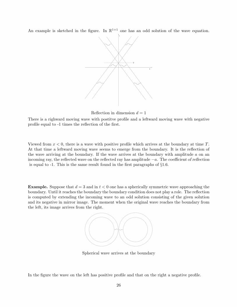
An example is sketched in the figure. In R1+1 one has an odd solution of the wave equation.

T

x

t

Reflection in dimension d = 1

There is a righward moving wave with postitve profile and a leftward moving wave with negativeprofile equal to -1 times the reflection of the first.

Viewed from x < 0, there is a wave with positive profile which arrives at the boundary at time T .At that time a leftward moving wave seems to emerge from the boundary. It is the reflection ofthe wave arriving at the boundary. If the wave arrives at the boundary with amplitude a on anincoming ray, the reflected wave on the reflected ray has amplitude !a. The coe!cient of reflectionis equal to -1. This is the same result found in the first paragraphs of §1.6.

Example. Suppose that d = 3 and in t < 0 one has a spherically symmetric wave approaching theboundary. Until it reaches the boundary the boundary condition does not play a role. The reflectionis computed by extending the incoming wave to an odd solution consisting of the given solutionand its negative in mirror image. The moment when the original wave reaches the boundary fromthe left, its image arrives from the right.

Spherical wave arrives at the boundary

In the figure the wave on the left has positive profile and that on the right a negative profile.

26

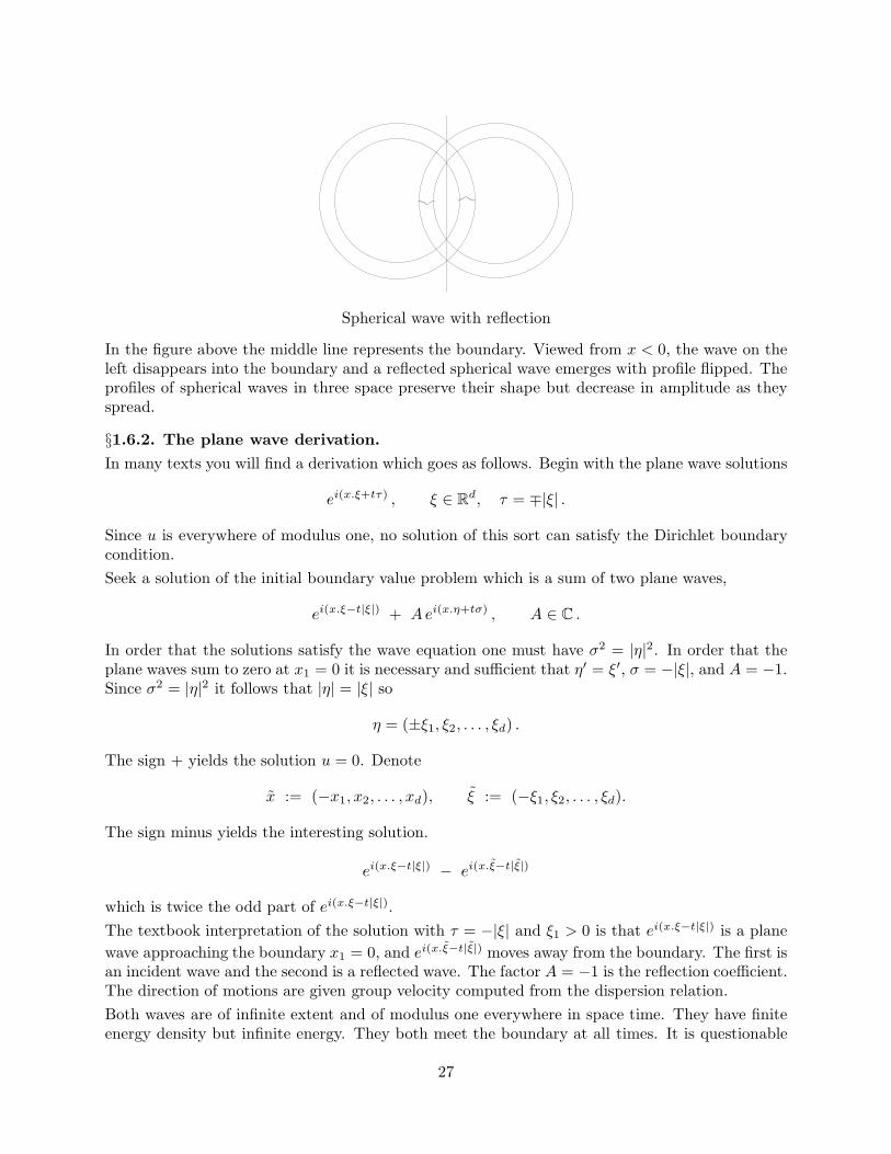
Spherical wave with reflection

In the figure above the middle line represents the boundary. Viewed from x < 0, the wave on theleft disappears into the boundary and a reflected spherical wave emerges with profile flipped. Theprofiles of spherical waves in three space preserve their shape but decrease in amplitude as theyspread.

§1.6.2. The plane wave derivation.

In many texts you will find a derivation which goes as follows. Begin with the plane wave solutions

ei(x.!+t$) , " ' Rd, # = "|"| .

Since u is everywhere of modulus one, no solution of this sort can satisfy the Dirichlet boundarycondition.

Seek a solution of the initial boundary value problem which is a sum of two plane waves,

ei(x.!!t|!|) + Aei(x.&+t') , A ' C .

In order that the solutions satisfy the wave equation one must have -2 = |*|2. In order that theplane waves sum to zero at x1 = 0 it is necessary and su!cient that *' = "', - = !|"|, and A = !1.Since -2 = |*|2 it follows that |*| = |"| so

* = (±"1, "2, . . . , "d) .

The sign + yields the solution u = 0. Denote

x := (!x1, x2, . . . , xd), " := (!"1, "2, . . . , "d).

The sign minus yields the interesting solution.

ei(x.!!t|!|) ! ei(x.!!t|!|)

which is twice the odd part of ei(x.!!t|!|).

The textbook interpretation of the solution with # = !|"| and "1 > 0 is that ei(x.!!t|!|) is a plane

wave approaching the boundary x1 = 0, and ei(x.!!t|!|) moves away from the boundary. The first isan incident wave and the second is a reflected wave. The factor A = !1 is the reflection coe!cient.The direction of motions are given group velocity computed from the dispersion relation.

Both waves are of infinite extent and of modulus one everywhere in space time. They have finiteenergy density but infinite energy. They both meet the boundary at all times. It is questionable

27

to think of either one as incoming or reflected. The next subsection shows that there are localizedwaves which are clearly incoming and reflected waves with the property that when they interactwith the boundary the local behavior resembles the plane waves.

For more general mixed initial boundary value problems, there are other wave forms which needto be included. The key is that solutions of the form ei(x.!+t$) are acceptable in x1 < 0 for "', #real and Im "1 , 0. When Im "1 < 0 the associated waves are localized near the boundary. TheRayleigh waves in elasticity are a classic example. They carry the devastating energy of earthquakes. Waves of this sort which do not propagate are needed to analyse total reflection which isdescribed at the end of §1.7. The reader is referred to [Benzoni-Gavage - Serre], [Chazarain-Piriou],[Taylor 1981], [Hormander 1982 v.II], [Sakamoto], for more information.

§1.6.3. Reflected high frequency wave packets.

Consider solutions which for small time are equal to high frequency solutions from §1.3,

u" = ei(x.!!t|!|)/" a(%, t, x) , a(%, t, x) . a0(t, x) + % a1(t, x) + · · · , (1.6.5)

with" = ("1, "2, . . . , "d) , "1 > 0 .

Then a0(t, x) = h(x! t"/|"|) is constant on the rays x+ t"/|"|. If the Cauchy data are supportedin a set O 22 {x1 < 0} then the amplitudes aj are supported in the tube of rays

T :=,

(t, x) : x = x + t"/|"|, x ' O-

, (1.6.6)

Finite speed shows that the wave as well as the geometric optics approximation stays strictly tothe left of the boundary for small t > 0.

The method of images computes the reflection. Define v" to be the reversed mirror image solution,

v"(t, x1, x2, . . . , xd) := !u"(t,!x1, x2, . . . , xd) .

The solution of the Dirichlet problem is then equal to the restriction of u" + v" to {x1 , 0}.Then

v" = ! ei(x.!!t)/" h(x! t") + h.o.t = ! ei(x.!!t)/" h(x ! t") + h.o.t .

To leading order, u" + v" is equal to

ei(x.!!t)/" h(x! t") ! ei(x.!!t)/" h(x ! t") . (1.6.7)

The wave represented by u" has leading term which moves with velocity "/|"|. The wave corre-sponding to v" has leading term with velocity "/|"|. which comes from "/|"| by reversing the firstcomponent. At the boundary x1 = 0, the tangential components of "/|"| and "/|"| are equal andtheir normal components are opposite. The directions are related by the standard law that theangle of incidence equals the angle of reflection. The amplitude of the reflected wave v" on thereflected ray is equal to !1 time the amplitude of the incoming wave u" on the incoming wave.This is summarized by the statement that the reflection coe!cient is equal to !1.

Suppose that t, x is a point on the boundary and O in a neighborhood of size large compared tothe wavelength % and small compared to the scale on which h varies. Then, on O, the solution isapproximately equal to

ei(x.!!t)/" h(x ! t"/|"|) ! ei(x.!!t)/" h(x ! t"/|"|) .

28

This recovers the reflected plane waves of §1.6.2. An observer on such an intermediate scale seesthe structure of the plane waves. Thus, even though the plane waves are completely nonlocal, theasymptotic solutions of geometric optics shows that they predict the local behavior at points ofreflection.

The method of images also solves the Neumann boundary value problem in a half space using evenmirror reflection in x1 = 0. It shows that for the Neumann condition, the reflection coe!cient isequal to 1.

Proposition 1.6.2. i. If u ' C$(R1+d) is an even solution of u = 0, then its restiction to{x1 , 0} is a smooth solution of u = 0 satisfying the Neumann boundary condition

!1u|x1=0 = 0 , (1.6.8)

ii. Conversely, if u ' C$({x1 , 0}) is a smooth solution of u = 0 satisfying (1.6.8) then theeven extension of u to R1+d is a smooth odd solution of u = 0.

The analogue of (1.6.3) in this case is

1n - 0,!2n+1u

!x2n+11

%%%%x1=0

= 0 . (1.6.9)

Exercise 1.6.1. Prove the Proposition.

Exercise 1.6.2. Prove uniqueness of solutions by the energy method. Hint. Use the local energyidentity.

Exercise 1.6.3 Verify the assertion concerning the reflection coe!cient by following the examplesabove. That is, consider the case of dimension d = 1, the case of spherical waves with d = 3 andthe behavior in the future of a solution which near t = 0 is a high frequency asymptotic solutionapproaching the boundary.

§1.7. Snell’s law of refraction.

Refraction is the bending of waves as they pass through media whose propagation speeds vary frompoint to point. The simplest situation is when media with di#erent speeds occupy half spaces, forexample x1 < 0 and x1 > 0. The classical physical situations are when light passes from air towater or from air to glass. It is observed that the angles of incidence and refraction are so that forfixed materials the ratio sin .i/ sin .r is independent of the incidence angle. Fermat observed thatthis would hold if the speed of light were di#erent in the two media and light light path was a pathof least time. In that case, the quotient of sines equal to the ratio of the speeds, ci/cr. In thissection we derive this behavior for a model problem quite close to the natural Maxwell equations.

The simplified model with the same geometry is,

utt !"u = 0 in x1 < 0 , utt ! c2 "u = 0 in x1 > 0 , 0 < c < 1 . (1.7.1)

In x1 < 0 the speed is equal to 1 which is greater than the speed c in x > 0. To see that c is the speedof the latter equation one can factor the one dimensional operator !2

t ! c2!2x = (!t = c!x)(!t! c!x)

or use the formula for group velocity with dispersion relation #2 = |"|2.A transmission condition is required at x1 = 0 to encode the interaction of waves with the interface.In the one dimesional case, there are waves which approach the boundary from both sides. The

29

waves which move from the boundary into the interior must be determined from the waves whicharrive from the interior. There are two arriving waves and two departing waves. One needs twoboundary conditions.

We analyse the transmission condition that imposes continuity of u and !1u across {x1 = 0}. Seeksolutions of (1.7.1) satsifying the transmission condition,

u(t, 0!, x') = u(t, 0+, x') , !1u(t, 0!, x') = !1u(t, 0+, x') . (1.7.2)

Denote by square brackets the jump

0u1(t, x') := u(t, 0+, x') ! u(t, 0!, x') .

The transmission condition is then

0u1

= 0 ,0!1u

1= 0 .

For solutions which are smooth on both sides of the boundary {x1 = 0}, the transmission condition(1.7.2) and be di#erentiated in t or x2, . . . , xd to find

2!(

t,x$u3

= 0 ,2!(

t,x$!1u3

= 0 . (1.7.3)

The partial di#erential equations then imply that in x1 < 0 and x1 > 0 respectively one has

!2u

!x21

=!2u

!t2!

d!

j=2

!2u

!x2j

,!2u

!x21

=1

c2

!2u

!t2!

d!

j=2

!2u

!x2j

,

Therefore at the boundary 4!2u

!x21

5=

&1 !

1

c2

)!2u

!t2.

The second derivative !21u is expected to be discontinuous at {x1 = 0}.

The physical conditions for Maxwell’s Equations at an air-water or air-glass interface can be anal-ysed in the same way. In that case, the dielectric constant is discontinuous at the interface.

Define

&(x) :=

67

8

1 when x1 > 0

c!2 when x1 < 0 ,e(t, x) :=

& u2t + |#xu|2

2,

From (1.7.1) it follows that solutions suitably small at infinity satisfy

!t

"

x1<0e dx =

"ut(t, 0

!, x') !1u(t, 0+, x') dx' ,

!t

"

x1>0e dx = !

"ut(t, 0

+, x') !1u(t, 0+, x') dx' .

The transmission condition guarantees that the terms on the right compensate exactly so

!t

"

R3

e dx = 0 .

30

This su!ces to prove uniqueness of solutions. A localized argument as in §1.6.1, shows that signalstravel at most at speed one.

Exercise 1.7.1. Prove this finite speed result.

A function u(t, x) is called piecewise smooth if its restriction to x1 < 0 (resp. x1 > 0) has aC$ extension to x1 , 0 (resp. x1 - 0). The Cauchy data of piecewise smooth solutions must bepiecewise smooth (with the analogous definition for functions of x only). They must, in addition,satisfy conditions analogous to (1.6.3).

Propostion 1.7.1. If u is a piecewise smooth solutions u of the transmission problem, then thepartial derivatives satisfy the sequence of compatibility conditions, for all j - 0,

"j{u, ut}(t, 0!, x2, x3) = (c2")j{u, ut}(t, 0+, x2, x3) ,

"j!1{u, , ut}(t, 0!, x2, x3) = (c2")j!1{u, ut}(t, 0+, x2, x3) .

ii. Conversely, if the piecewise smooth f, g satisfy for all j - 0,

"j{f, g}(0!, x2, x3) = (c2")j{f, g}(0+, x2, x3) , (1.7.4)

"j!1{f, g}(0!, x2, x3) = (c2")j!1{f, g}(0+, x2, x3) , (1.7.5)

then there is a piecewise smooth solution with these Cauchy data.

Proof. i. If u is a piecewise smooth solution then so is !jt u for any j. Use (1.7.2) for pure time

derivatives, 0!j

t u1

= 0 ,0!j

t !1u1

= 0 . (1.7.6)

The case j = 1 yields the necessary condition

0g1

= 0 ,0!1g

1= 0 .

For the higher orders, compute with k - 1,

!2kt u

%%t=0

=

67

8

"ku when x1 < 0

(c2")ku when x1 > 0,

!2k!1t u

%%t=0

=

67

8

"ku when x1 < 0

(c2")ku when x1 > 0.

Thus, the transmission conditions (1.7.6) proves i.

The proof of ii. is technical, interesting, and omitted. One can construct solutions using finitedi#erences almost as in §2.2. The shortest existence proof to state uses the spectral theorem for selfadjoint operators.( The general regularity theory for such transmission problems can be obtained

( For those with su!cient background, the Hilbert space is H := L2(Rd ; & dx).

D(A) :=,w ' H2(Rd

+) ( H2(Rd!) : [w] = [!1w] = 0

-,

31

by folding them to a boundary value problem and using the results of [Rauch-Massey, Sakamoto].

Next consider the mathematical problem whose solution explains Snell’s law. The idea is to senda wave in x1 < 0 toward the boundary and ask how it behaves in the future. Suppose

" ' Rd, |"| = 1 , "1 > 0 ,

and consider a short wavelength asymptotic solution in {x1 < 0} as in §1.6.3,

I" . ei(x.!!t)/" a(%, t, x) , a(%, t, x) . a0(t, x) + % a1(t, x) + · · · , (1.7.5)

where for t < 0 the support of the aj is contained in a tube of rays with compact cross sectionand moving with speed ". One can take a to vanish outside the tube. Since the incoming wavesare smooth and initially vanish identically on a neighborhood of the interface {x1 = 0}, thecompatibilities are satisfied and there is a family of piecewise smooth solutions u" defined on R1+d.The tools prepared yield an infinitely accurate description of the family of solutions u".

To solve the problem, seek an asymptotic solution which at {t = 0} is equal to this incoming wave.A first idea is to find a transmitted wave which continues the incoming wave into {x1} > 0.

Seek the transmitted wave in x1 > 0 in the form

T " . ei(x.&+t$)/" d(%, t, x) , d(%, t, x) . d0(t, x) + % d1(t, x) + · · · ,

In order that this be an approximate solution moving away from the interface one must have

#2 = c2|*|2, |*| = 1/c .

The incoming wave, when restricted to the interface x1 = 0 oscillates with phase (x'."' ! t)/%. Atthe interface, the proposed transmitted wave oscillates with phase (x'.*' ! t#)/%. In order thatthere be any chance at all of satisfying the transmission condtions one must take

*' = "', # = !1,

so that the two expressions oscillate together.

Aw := "w in x1 < 0, Aw := c2" in x1 > 0 .

Then,

(Au, v)H = (u,Av)H = !"

#u.#v dx ,

so !A - 0. The elliptic regularity theorem implies that A is self adjoint. The regularity theoremis proved, for example, by the methods in [Rauch 1992, Chapter 10]. The solution of the initialvalue problem is

u = cos t0!A f +

sin t0!A0

!Ag .

For piecwise H$ data, the sequence of compatibilities is equivalent to the data belonging to(jD(Aj).

32

The equation #2 = c2|*|2 implies

*21 =

#2

c2! |*'|2 =

1

c2! |"'|2 .

Impose *1 > 0 so the transmitted wave moves into the region x1 > 0 to find

*1 =

&1

c2! |"'|2

)1/2

> "1.

Thus,

T " . ei(x.&!t)/" d(%, t, x) , * =

&&1

c2! |"'|2

)1/2

, "')

. (1.7.6)

From section 1.6.3 we know that the leading amplitude d0 must be constant on the rays t /*(t, x + c t */|*|). To determine d0 it su!ces to know the values d0(t, 0+, x') at the interface. Onecould choose d0 to guarantee the continuity of u or of !1u, but not both. One cannot construct angood approximated solution consisting of just an incident and transmitted wave.

Add to the recipe a reflected wave. Seek a reflected wave in x1 - 0 in the form

R" . ei(x.#+t')/" b(%, t, x) , b(%, t, x) . b0(t, x) + % b1(t, x) + · · · .

In order that the reflected wave oscillate with the same phase as the incident wave in the boundaryx1 = 0, one must have ' ' = "' and - = !1. To satisfy the wave equation in x1 < 0 requires-2 = |'|2. Together these imply '2

1 = "21 . To have propagation away from the boundary requires

'1 = !"1 so ' = ". Therefore,

R" . ei(x.!!t)/" b(%, t, x) , b(%, t, x) . b0(t, x) + % b1(t, x) + · · · . (1.7.7)

Summarizing seek

v" =

9I" + R" in x1 < 0

T " in x1 > 0.

The continuity required at x1 = 0 forces

ei(x$.!$!t)/" (a(%, t, 0, x') + b(%, t, 0, x')) = ei(x$.!$!t)/" d(%, t, 0, x') . (1.7.8)

The continuity of u and !1u hold if and only if at x1 = 0 one has

a + b = d , and,i"1

%a + !1a !

i"1

%b + !1b =

i*1

%d + !1d . (1.7.9)

The first of these relations yields

'aj + bj ! dj

(

x1=0= 0, j = 0, 1, 2, . . . , (1.7.10)

The second relation in (1.7.9) is expanded in powers of %. The coe!cients of %j must match for allall j - !1. The leading order is %!1 and yields

#a0 ! b0 ! (*1/"1)d0

$x1=0

= 0 . (1.7.11)

33

Since a0 is known, the j = 0 equation from (1.7.10) together with (1.7.11) yield a system of twolinear equations for the two unknown b0, d0

&!1 11 *1/"1

) &b0

d0

)=

&a0

a0

).

Since the matrix is invertible, this determines the values of b0 and d0 at x1 = 0.

The amplitude b0 (resp. d0) is constant on rays with velocity " (resp. c*/|*|). Thus the leadingamplitudes are determined throughout the half spaces on which they are defined.

Once these leading terms are known the %0 term from the second equation in (1.7.9) shows that onx1 = 0,

a1 ! b1 ! d1 = known .

Note that a1 is also known so that together with the case j = 2 from (1.7.10) this su!ces todetermine b1, d1 on x1 = 0. Each satisfies a transport equation along rays which is the analogue of(1.4.12). Thus from the initial values just computed on x1 = 0 they are determined everywhere.The higher order correctors are detemined analogously.

Once the bj , dj are determined, one can choose b, c as functions of % with the known Taylor ex-pansions at x = 0. They can be chosen to have supports in the appropriate tubes of rays and tosatisfy the transmission conditions (1.7.9) exactly.

The function u" is then an infinitely accurate approximate solution in the sense that it satisfies thetransmission and initial conditions exactly while the residuals

v"tt !" v" := r" in x1 < 0 , v"

tt ! c2 " v" := /",

satisfy for all N, s, T there is a C so that

++r"++

Hs([!T,T ]){x1<0})+

++/"++

Hs([!T,T ]){x1>0}), C %N .

From the analysis of the transmission problem it follows that with new constants,

++u" ! v"++

Hs([!T,T ]){x1>0}), C %N .

The proposed problem of describing the family of solutions u" is solved.

The angles of incidence and refraction, .i and .r, given by the directions of propagation of theincident and transmitted waves. From the figure

’

ξ ’

ξ

η

η

one finds,

sin .i =|"'||"|

, and, sin .r =|*'||*|

=|"'||"|/c

.

34

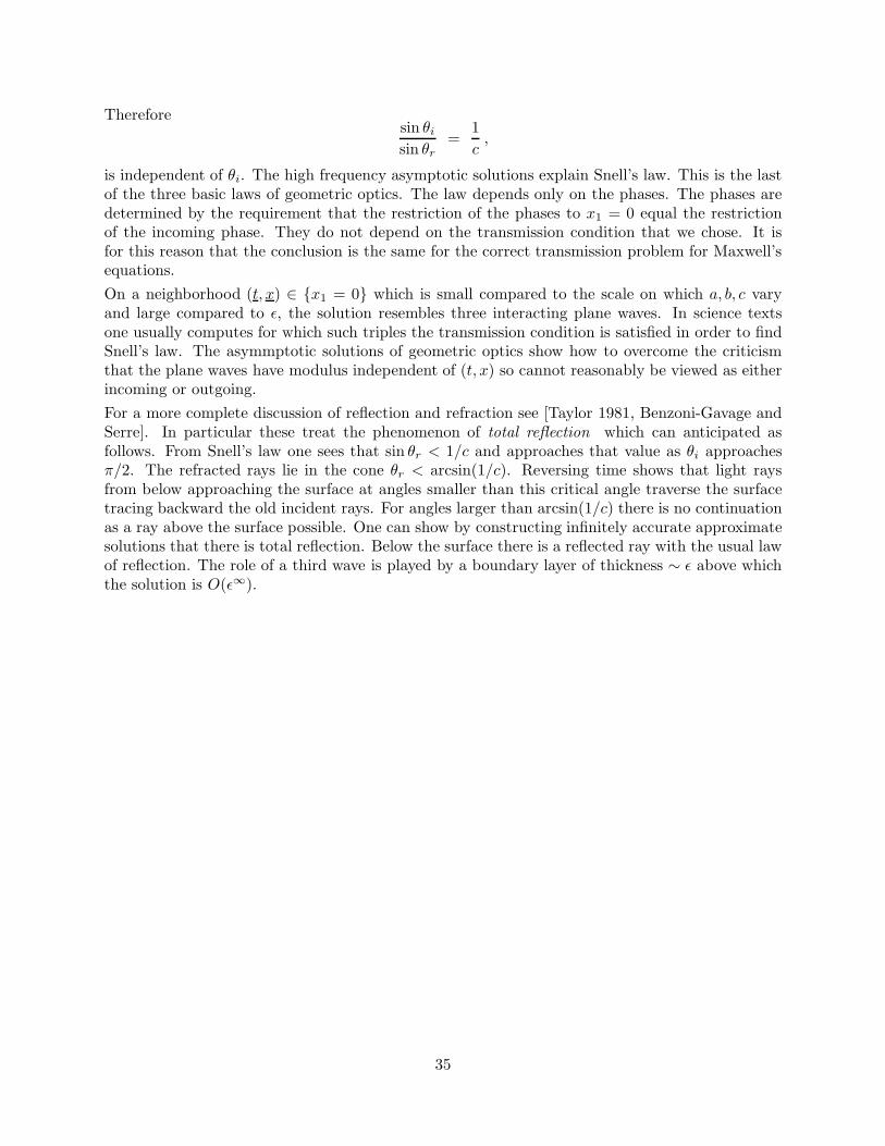
Thereforesin .i

sin .r=

1

c,

is independent of .i. The high frequency asymptotic solutions explain Snell’s law. This is the lastof the three basic laws of geometric optics. The law depends only on the phases. The phases aredetermined by the requirement that the restriction of the phases to x1 = 0 equal the restrictionof the incoming phase. They do not depend on the transmission condition that we chose. It isfor this reason that the conclusion is the same for the correct transmission problem for Maxwell’sequations.

On a neighborhood (t, x) ' {x1 = 0} which is small compared to the scale on which a, b, c varyand large compared to %, the solution resembles three interacting plane waves. In science textsone usually computes for which such triples the transmission condition is satisfied in order to findSnell’s law. The asymmptotic solutions of geometric optics show how to overcome the criticismthat the plane waves have modulus independent of (t, x) so cannot reasonably be viewed as eitherincoming or outgoing.

For a more complete discussion of reflection and refraction see [Taylor 1981, Benzoni-Gavage andSerre]. In particular these treat the phenomenon of total reflection which can anticipated asfollows. From Snell’s law one sees that sin .r < 1/c and approaches that value as .i approaches$/2. The refracted rays lie in the cone .r < arcsin(1/c). Reversing time shows that light raysfrom below approaching the surface at angles smaller than this critical angle traverse the surfacetracing backward the old incident rays. For angles larger than arcsin(1/c) there is no continuationas a ray above the surface possible. One can show by constructing infinitely accurate approximatesolutions that there is total reflection. Below the surface there is a reflected ray with the usual lawof reflection. The role of a third wave is played by a boundary layer of thickness . % above whichthe solution is O(%$).

35