Textures on Rank-1 Lattices

S. Dammertz1 and H. Dammertz1 and A. Keller2 and H. P. A. Lensch3

1(sabrina, holger).dammertz@uni-ulm.de Ulm University, Germany2alex@mental.com, mental images GmbH, Germany

3hendrik.lensch@uni-ulm.de Ulm University, Germany

Figure 1: Comparison of standard textures with rank-1 lattice textures where each image contains thesame number of picture elements (64× 64). Rank-1 lattices can very closely approximate the hexagonallattice. This reduces aliasing and results, among other things, in an improved reproduction of non axis-parallel lines as can be seen clearly in the middle image.

Abstract

Storing textures on orthogonal tensor product lattices is pre-dominant in computer graphics, although it is known that theirsampling efficiency is not optimal. In two dimensions, thehexagonal lattice provides the maximum sampling efficiency.However, handling these lattices is difficult, because they arenot able to tile an arbitrary rectangular region and have anirrational basis. By storing textures on rank-1 lattices, we re-solve both problems: Rank-1 lattices can closely approximatehexagonal lattices, while all coordinates of the lattice pointsremain integer. At identical memory footprint texture qualityis improved as compared to traditional orthogonal tensor prod-uct lattices due to the higher sampling efficiency. We introducethe basic theory of rank-1 lattice textures and present an algo-rithmic framework which easily can be integrated into existingoff-line and real-time rendering systems.

1. Introduction

The traditional orthogonal equidistant lattice with its squaretexture elements is far from optimal for storing and displayinggeneral images. In the context of sampling for signal processingthis has been recognized already very early by Petersen et al.[PM62]. They quantify the quality of a sampling lattice by itssampling efficiency

η :=R

P,

where R is the area of the in-circle of the fundamental Voronoicell and P denotes the volume of the fundamental Voronoi cellitself in the dual lattice. The sampling efficiency measures howwell the sampling points of a given lattice capture the isotropicspectrum of a band-limited function. In this context a samplingefficiency of 100% would allow to perfectly represent the band-limited function. Petersen et al. derive the optimal samplinglattices for up to 8 dimensions. While in 2D the optimal latticeis the well known hexagonal lattice with η = 90.7%, the 2Dsquare lattice has a sampling efficiency of only η = 78.5%.

Hexagonal sampling lattices have been investigated for morethan 40 years, giving rise to the field of hexagonal image pro-cessing. With applications in medicine, cameras, or hexagonaldisplays, hexagonal image processing (HIP) is an active field in

0

1

0

1

2

3

4

5

6

0

1

2

3

4

5

6

7

b1

b2

g

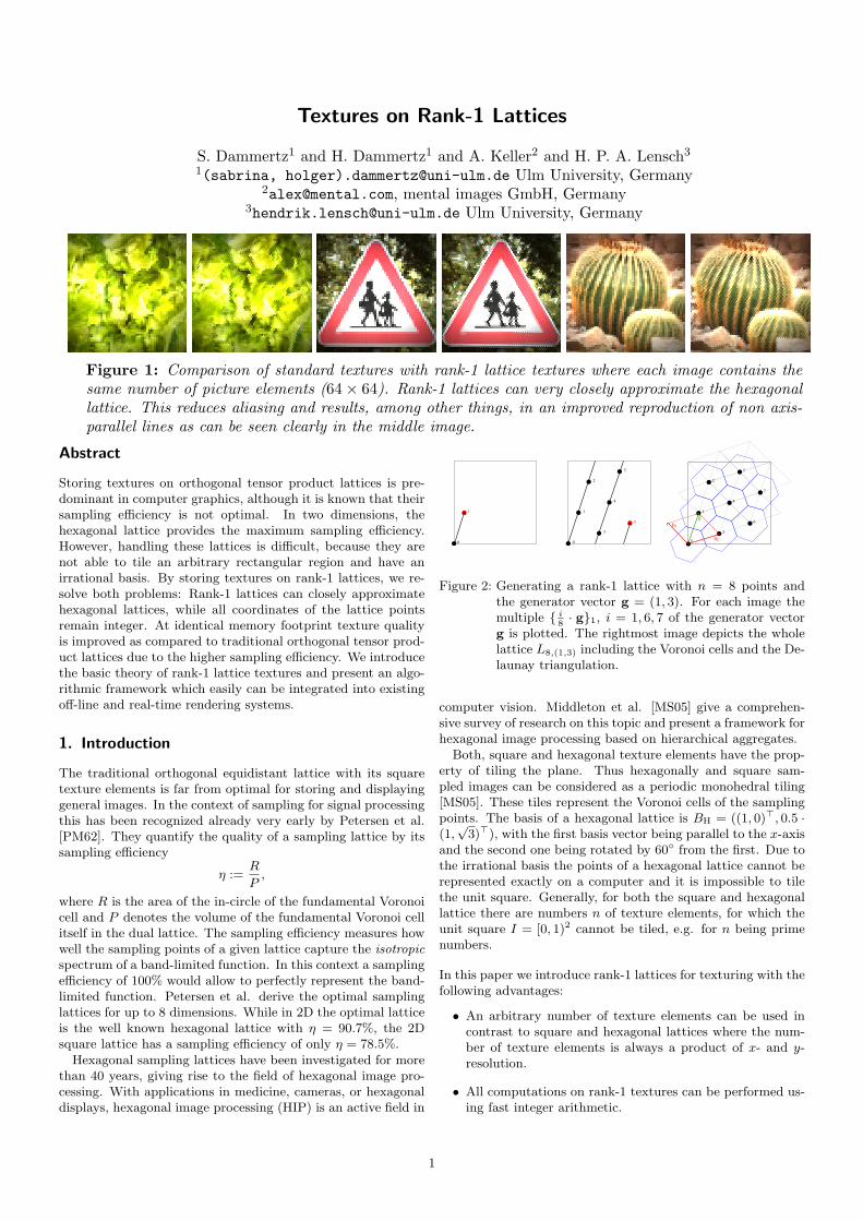
Figure 2: Generating a rank-1 lattice with n = 8 points andthe generator vector g = (1, 3). For each image themultiple { i

8· g}1, i = 1, 6, 7 of the generator vector

g is plotted. The rightmost image depicts the wholelattice L8,(1,3) including the Voronoi cells and the De-launay triangulation.

computer vision. Middleton et al. [MS05] give a comprehen-sive survey of research on this topic and present a framework forhexagonal image processing based on hierarchical aggregates.

Both, square and hexagonal texture elements have the prop-erty of tiling the plane. Thus hexagonally and square sam-pled images can be considered as a periodic monohedral tiling[MS05]. These tiles represent the Voronoi cells of the samplingpoints. The basis of a hexagonal lattice is BH = ((1, 0)>, 0.5 ·(1,

√3)>), with the first basis vector being parallel to the x-axis

and the second one being rotated by 60◦ from the first. Due tothe irrational basis the points of a hexagonal lattice cannot berepresented exactly on a computer and it is impossible to tilethe unit square. Generally, for both the square and hexagonallattice there are numbers n of texture elements, for which theunit square I = [0, 1)2 cannot be tiled, e.g. for n being primenumbers.

In this paper we introduce rank-1 lattices for texturing with thefollowing advantages:

• An arbitrary number of texture elements can be used incontrast to square and hexagonal lattices where the num-ber of texture elements is always a product of x- and y-resolution.

• All computations on rank-1 textures can be performed us-ing fast integer arithmetic.

1

• The new texture scheme provides a close rational approx-imation to hexagonal textures for any resolution (evenpower of 2). We also show the equivalence of hexagonaland rank-1 textures for a subset of rank-1 lattices.

• We provide the necessary theory and algorithms to effi-ciently implement rank-1 textures into any rendering sys-tem.

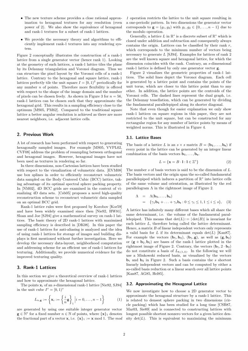
Figure 2 conceptually illustrates the construction of a rank-1lattice from a single generator vector (hence rank 1). Lookingat the geometry of such lattices, a rank-1 lattice tiles the planeby its Delaunay triangulation and Voronoi diagram. Thus wecan structure the pixel layout by the Voronoi cells of a rank-1lattice. Contrary to the hexagonal and square lattice, rank-1lattices perfectly tile the unit square I = [0, 1)2 periodically forany number n of points. Therefore more flexibility is offeredwith respect to the shape of the image domain and the numberof pixels can be chosen freely. As shown in Figure 3 for n = 56,rank-1 lattices can be chosen such that they approximate thehexagonal grid. This results in a sampling efficiency close to theoptimum [MS05, PM62]. Compared to the traditional squarelattice a better angular resolution is achieved as there are morenearest neighbors, i.e. adjacent lattice cells.

2. Previous Work

A lot of research has been performed with respect to generatinghexagonally sampled images. For example [MS05, VVPL02,CVF08] address the problem of resampling between orthogonaland hexagonal images. However, hexagonal images have notbeen used as textures in rendering so far.

In three dimensions, non-Cartesian lattices have been studiedwith respect to the visualization of volumetric data. [EVM08]use box splines in order to efficiently reconstruct volumetricdata sampled on the Body Centered Cubic (BCC) lattice, tak-ing advantage of its optimal spectral sphere packing property.In [NM02], 4D BCC grids are examined in the context of vi-sualizing 4D data sets. [Csb05] proposes a novel high-qualityreconstruction scheme to reconstruct volumetric data sampledon an optimal BCC grid.

Rank-1 lattice rules were first proposed by Korobov [Kor59]and have been widely examined since then [Nie92, HW81].Sloan and Joe [SJ94] give a mathematical survey on rank-1 lat-tices. The basic theory of 2D rank-1 lattices with maximizedsampling efficiency is described in [DK08]. In this paper theuse of rank-1 lattices for anti-aliasing is analyzed and the ideaof using rank-1 lattices for storage of images and building dis-plays is first mentioned without further investigation. Here wedevelop the necessary data-layout, neighborhood computationand addressing scheme for an efficient use of rank-1 lattices fortexturing. Additionally, we provide numerical evidence for theimproved texturing quality.

3. Rank-1 Lattices

In this section we give a theoretical overview of rank-1 latticesand how to approximate the hexagonal lattice.

The points xi of an s-dimensional rank-1 lattice [Nie92, SJ94]in the unit cube Is = [0, 1)s

Ln,g :=

xi :=

i

ng

ff1

˛i = 0, . . . , n− 1

ff(1)

are generated by using one suitable integer generator vectorg ∈ Ns for a fixed number n ∈ N of points, where {x}1 denotesthe fractional part of a vector x, i.e. {x}1 := x mod 1. The mod

1 operation restricts the lattice to the unit square resulting ina one-periodic pattern. In two dimensions the generator vectorcorresponds to g = (g1, g2) with g1, g2 ∈ {0, . . . , n − 1} due tothe modulo operation.

Generally, a lattice L in Rs is a discrete subset of Rs which isclosed under addition and subtraction and consequently alwayscontains the origin. Lattices can be classified by their rank r,which corresponds to the minimum number of vectors beingnecessary to generate L [SJ94]. Examples for lattices of rank 2are the well known square and hexagonal lattice, for which thedimension coincides with the rank. Contrary, an s-dimensionalrank-1 lattice is defined by only one generator vector g.

Figure 2 visualizes the geometric properties of rank-1 lat-tices. The solid lines depict the Voronoi diagram. Each cellis generated by a lattice point and contains the points of theunit torus, which are closer to this lattice point than to anyother. In addition, the lattice points are the centroids of theVoronoi cells. The dashed lines represent the dual graph, i.e.the Delaunay tessellation, which can be generated by dividingthe fundamental parallelepiped along its shorter diagonal.

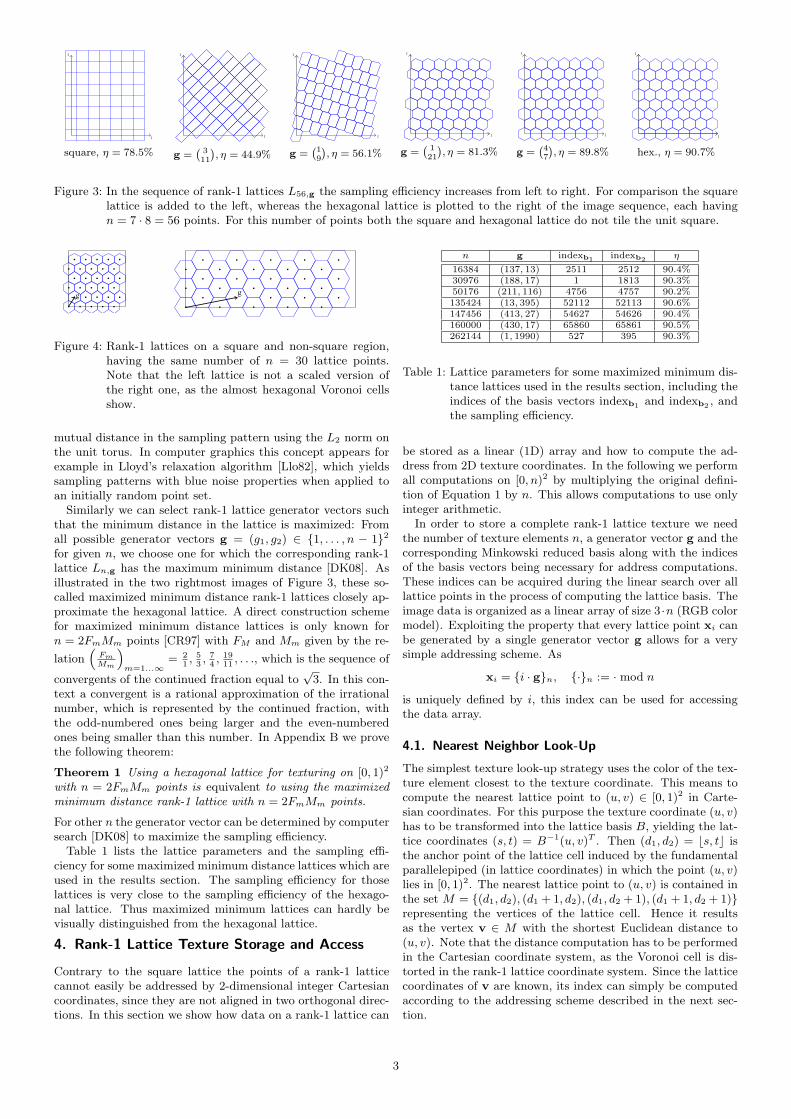
Note that even though for easier explanation we only showrank-1 lattices on square regions in this paper, they are notrestricted to the unit square, but can be constructed for anyrectangular region for any number of lattice points by means ofweighted norms. This is illustrated in Figure 4.

3.1. Lattice Bases

The basis of a lattice L is an s × s matrix B = (b1, . . . ,bs) ifevery point in the lattice can be generated by an integer linearcombination of the basis vectors b1, . . . ,bs.

L = {x = B · l : l ∈ Zs} (2)

The number s of basis vectors is said to be the dimension of L.The basis vectors and the origin span the so-called fundamentalparallelepiped which induces a partition of Rs into lattice cellsof the same volume and orientation, as illustrated by the redparallelogram Λ in the rightmost image of Figure 2.

Λ = Λ(b1, . . . ,bs)

= {γ1b1 + . . . + γsbs : 0 ≤ γi ≤ 1, 1 ≤ i ≤ s}, (3)

A lattice has infinitely many different bases which all share thesame determinant, i.e. the volume of the fundamental paral-lelepiped. This means that det(L) := | det(B)| is invariant foreach lattice L, therefore being called the lattice determinant.Hence, a matrix B of linear independent vectors only representsa valid basis for L if its determinant equals det(L) [Kan87].For example the vectors (b1,b2), (b1,g), as well as (g,b2)or (g + b2,b2) are bases of the rank-1 lattice plotted in therightmost image of Figure 2. Contrary, the vectors (b1, 2 · b2)do not constitute a basis of L8,(1,3). In the following we willuse a Minkowski reduced basis, as visualized by the vectorsb1 and b2 in Figure 2. Such a basis contains the s shortestlinearly independent vectors and can be computed by either aso-called basis reduction or a linear search over all lattice points[Kan87, AG85, Hel85].

3.2. Approximating the Hexagonal Lattice

We now investigate how to choose a 2D generator vector toapproximate the hexagonal structure by a rank-1 lattice. Thisis related to densest sphere packing in two dimensions (cir-cle packing) which has been studied for a long time [CSB87,Mar03, Sie89] and is connected to constructing lattices withlongest possible shortest nonzero vectors for a given lattice den-sity det(L). This is equivalent to maximizing the minimum

2

1

1

square, η = 78.5%

1

1

g =` 311

´, η = 44.9%

1

1

g =`19

´, η = 56.1%

1

1

g =` 121

´, η = 81.3%

1

1

g =`47

´, η = 89.8%

1

1

hex., η = 90.7%

Figure 3: In the sequence of rank-1 lattices L56,g the sampling efficiency increases from left to right. For comparison the squarelattice is added to the left, whereas the hexagonal lattice is plotted to the right of the image sequence, each havingn = 7 · 8 = 56 points. For this number of points both the square and hexagonal lattice do not tile the unit square.

g g

Figure 4: Rank-1 lattices on a square and non-square region,having the same number of n = 30 lattice points.Note that the left lattice is not a scaled version ofthe right one, as the almost hexagonal Voronoi cellsshow.

mutual distance in the sampling pattern using the L2 norm onthe unit torus. In computer graphics this concept appears forexample in Lloyd’s relaxation algorithm [Llo82], which yieldssampling patterns with blue noise properties when applied toan initially random point set.

Similarly we can select rank-1 lattice generator vectors suchthat the minimum distance in the lattice is maximized: Fromall possible generator vectors g = (g1, g2) ∈ {1, . . . , n − 1}2

for given n, we choose one for which the corresponding rank-1lattice Ln,g has the maximum minimum distance [DK08]. Asillustrated in the two rightmost images of Figure 3, these so-called maximized minimum distance rank-1 lattices closely ap-proximate the hexagonal lattice. A direct construction schemefor maximized minimum distance lattices is only known forn = 2FmMm points [CR97] with FM and Mm given by the re-

lation“

FmMm

”m=1...∞

= 21, 5

3, 7

4, 19

11, . . ., which is the sequence of

convergents of the continued fraction equal to√

3. In this con-text a convergent is a rational approximation of the irrationalnumber, which is represented by the continued fraction, withthe odd-numbered ones being larger and the even-numberedones being smaller than this number. In Appendix B we provethe following theorem:

Theorem 1 Using a hexagonal lattice for texturing on [0, 1)2

with n = 2FmMm points is equivalent to using the maximizedminimum distance rank-1 lattice with n = 2FmMm points.

For other n the generator vector can be determined by computersearch [DK08] to maximize the sampling efficiency.

Table 1 lists the lattice parameters and the sampling effi-ciency for some maximized minimum distance lattices which areused in the results section. The sampling efficiency for thoselattices is very close to the sampling efficiency of the hexago-nal lattice. Thus maximized minimum lattices can hardly bevisually distinguished from the hexagonal lattice.

4. Rank-1 Lattice Texture Storage and Access

Contrary to the square lattice the points of a rank-1 latticecannot easily be addressed by 2-dimensional integer Cartesiancoordinates, since they are not aligned in two orthogonal direc-tions. In this section we show how data on a rank-1 lattice can

n g indexb1 indexb2 η

16384 (137, 13) 2511 2512 90.4%30976 (188, 17) 1 1813 90.3%50176 (211, 116) 4756 4757 90.2%135424 (13, 395) 52112 52113 90.6%147456 (413, 27) 54627 54626 90.4%160000 (430, 17) 65860 65861 90.5%262144 (1, 1990) 527 395 90.3%

Table 1: Lattice parameters for some maximized minimum dis-tance lattices used in the results section, including theindices of the basis vectors indexb1 and indexb2 , andthe sampling efficiency.

be stored as a linear (1D) array and how to compute the ad-dress from 2D texture coordinates. In the following we performall computations on [0, n)2 by multiplying the original defini-tion of Equation 1 by n. This allows computations to use onlyinteger arithmetic.

In order to store a complete rank-1 lattice texture we needthe number of texture elements n, a generator vector g and thecorresponding Minkowski reduced basis along with the indicesof the basis vectors being necessary for address computations.These indices can be acquired during the linear search over alllattice points in the process of computing the lattice basis. Theimage data is organized as a linear array of size 3 ·n (RGB colormodel). Exploiting the property that every lattice point xi canbe generated by a single generator vector g allows for a verysimple addressing scheme. As

xi = {i · g}n, {·}n := · mod n

is uniquely defined by i, this index can be used for accessingthe data array.

4.1. Nearest Neighbor Look-Up

The simplest texture look-up strategy uses the color of the tex-ture element closest to the texture coordinate. This means tocompute the nearest lattice point to (u, v) ∈ [0, 1)2 in Carte-sian coordinates. For this purpose the texture coordinate (u, v)has to be transformed into the lattice basis B, yielding the lat-tice coordinates (s, t) = B−1(u, v)T . Then (d1, d2) = bs, tc isthe anchor point of the lattice cell induced by the fundamentalparallelepiped (in lattice coordinates) in which the point (u, v)lies in [0, 1)2. The nearest lattice point to (u, v) is contained inthe set M = {(d1, d2), (d1 + 1, d2), (d1, d2 + 1), (d1 + 1, d2 + 1)}representing the vertices of the lattice cell. Hence it resultsas the vertex v ∈ M with the shortest Euclidean distance to(u, v). Note that the distance computation has to be performedin the Cartesian coordinate system, as the Voronoi cell is dis-torted in the rank-1 lattice coordinate system. Since the latticecoordinates of v are known, its index can simply be computedaccording to the addressing scheme described in the next sec-tion.

3

0

1

2

3

4

5

6

7

8

9

10

11

12

13

14

15

16

17

18

19

20

21

22

23

24

25

26

27

28

29

30

31

32

33

34

35

36

37

38

39

40

41

42

43

44

45

46

47

48

49

50

51

52

53

54

55

b1

b2

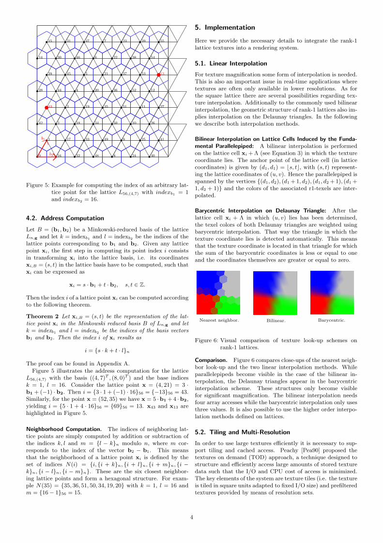
Figure 5: Example for computing the index of an arbitrary lat-tice point for the lattice L56,(4,7) with indexb1 = 1and indexb2 = 16.

4.2. Address Computation

Let B = (b1,b2) be a Minkowski-reduced basis of the latticeLn,g and let k = indexb1 and l = indexb2 be the indices of thelattice points corresponding to b1 and b2. Given any latticepoint xi, the first step in computing its point index i consistsin transforming xi into the lattice basis, i.e. its coordinatesxi,B = (s, t) in the lattice basis have to be computed, such thatxi can be expressed as

xi = s · b1 + t · b2, s, t ∈ Z.

Then the index i of a lattice point xi can be computed accordingto the following theorem.

Theorem 2 Let xi,B = (s, t) be the representation of the lat-tice point xi in the Minkowski reduced basis B of Ln,g and letk = indexb1 and l = indexb2 be the indices of the basis vectorsb1 and b2. Then the index i of xi results as

i = {s · k + t · l}n

The proof can be found in Appendix A.

Figure 5 illustrates the address computation for the latticeL56,(4,7) with the basis ((4, 7)T , (8, 0)T ) and the base indicesk = 1, l = 16. Consider the lattice point x = (4, 21) = 3 ·b1 + (−1) · b2. Then i = {3 · 1 + (−1) · 16}56 = {−13}56 = 43.Similarly, for the point x = (52, 35) we have x = 5 ·b1 + 4 ·b2,yielding i = {5 · 1 + 4 · 16}56 = {69}56 = 13. x43 and x13 arehighlighted in Figure 5.

Neighborhood Computation. The indices of neighboring lat-tice points are simply computed by addition or subtraction ofthe indices k, l and m = {l − k}n modulo n, where m cor-responds to the index of the vector b2 − b1. This meansthat the neighborhood of a lattice point xi is defined by theset of indices N(i) = {i, {i + k}n, {i + l}n, {i + m}n, {i −k}n, {i − l}n, {i − m}n}. These are the six closest neighbor-ing lattice points and form a hexagonal structure. For exam-ple N(35) = {35, 36, 51, 50, 34, 19, 20} with k = 1, l = 16 andm = {16− 1}56 = 15.

5. Implementation

Here we provide the necessary details to integrate the rank-1lattice textures into a rendering system.

5.1. Linear Interpolation

For texture magnification some form of interpolation is needed.This is also an important issue in real-time applications wheretextures are often only available in lower resolutions. As forthe square lattice there are several possibilities regarding tex-ture interpolation. Additionally to the commonly used bilinearinterpolation, the geometric structure of rank-1 lattices also im-plies interpolation on the Delaunay triangles. In the followingwe describe both interpolation methods.

Bilinear Interpolation on Lattice Cells Induced by the Funda-mental Parallelepiped: A bilinear interpolation is performedon the lattice cell xi + Λ (see Equation 3) in which the texturecoordinate lies. The anchor point of the lattice cell (in latticecoordinates) is given by (d1, d1) = bs, tc, with (s, t) represent-ing the lattice coordinates of (u, v). Hence the parallelepiped isspanned by the vertices {(d1, d2), (d1 + 1, d2), (d1, d2 + 1), (d1 +1, d2 + 1)} and the colors of the associated r1-texels are inter-polated.

Barycentric Interpolation on Delaunay Triangle: After thelattice cell xi + Λ in which (u, v) lies has been determined,the texel colors of both Delaunay triangles are weighted usingbarycentric interpolation. That way the triangle in which thetexture coordinate lies is detected automatically. This meansthat the texture coordinate is located in that triangle for whichthe sum of the barycentric coordinates is less or equal to oneand the coordinates themselves are greater or equal to zero.

Nearest neighbor. Bilinear. Barycentric.

Figure 6: Visual comparison of texture look-up schemes onrank-1 lattices.

Comparison. Figure 6 compares close-ups of the nearest neigh-bor look-up and the two linear interpolation methods. Whileparallelepipeds become visible in the case of the bilinear in-terpolation, the Delaunay triangles appear in the barycentricinterpolation scheme. These structures only become visiblefor significant magnification. The bilinear interpolation needsfour array accesses while the barycentric interpolation only usesthree values. It is also possible to use the higher order interpo-lation methods defined on lattices.

5.2. Tiling and Multi-Resolution

In order to use large textures efficiently it is necessary to sup-port tiling and cached access. Peachy [Pea90] proposed thetextures on demand (TOD) approach, a technique designed tostructure and efficiently access large amounts of stored texturedata such that the I/O and CPU cost of access is minimized.The key elements of the system are texture tiles (i.e. the textureis tiled in square units adapted to fixed I/O size) and prefilteredtextures provided by means of resolution sets.

4

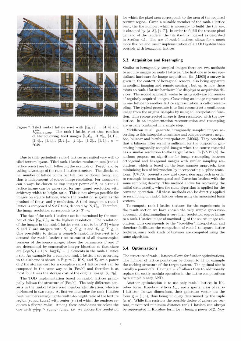
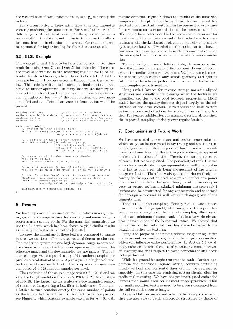
Figure 7: Tiled rank-1 lattice r-set with [S0, T0] = [4, 4] andLtile

2048,(31,39). The rank-1 lattice r-set thus consistsof the following tiled images [4, 4]n, [4, 2]n, [4, 1]n,[2, 4]n, [1, 4]n, [2, 2, ]n, [2, 1]n, [1, 2]n, [1, 1]n, n =2048.

Due to their periodicity rank-1 lattices are suited very well totiled texture layout. Tiled rank-1 lattice resolution sets (rank-1lattice r-sets) are built following the example of [Pea90] and bytaking advantage of the rank-1 lattice structure. The tile size n,i.e. number of lattice points per tile, can be chosen freely, andthus is independent of source image resolution. For example ncan always be chosen as any integer power of 2, as a rank-1lattice image can be generated for any target resolution witharbitrary width-to-height ratio. This is not always possible forimages on square lattices, where the resolution is given as theproduct of the x- and y-resolution. A tiled image on a rank-1lattice is composed of S×T tiles, denoted by [S, T ]n. Therefore,the image resolution corresponds to S · T · n.

The size of the rank-1 lattice r-set is determined by the num-ber of tiles [S0, T0]n in the highest resolution. The resolutionof the images in the rank-1 lattice r-set is set to be [S, T ] whereS and T are integers with S0 ≥ S ≥ 0 and T0 ≥ T ≥ 0.One possibility to define a complete rank-1 lattice r-set is todemand the rank-1 lattice r-set to consist of all downsampledversions of the source image, where the parameters S and Tare determined by consecutive integer bisection so that thereare blog(S0) + 1c × blog(T0) + 1c elements in the rank-1 latticer-set. An example for a complete rank-1 lattice r-set accordingto this scheme is shown in Figure 7. If S0 and T0 are a powerof 2 the storage cost for a complete rank-1 lattice r-set can becomputed in the same way as in [Pea90] and therefore is atmost four times the storage cost of the original image [S0, T0].

The TOD implementation based on rank-1 lattices princi-pally follows the structure of [Pea90]. The only difference con-sists in the rank-1 lattice r-set member identification, which isperformed in two steps. At first we determine the rank-1 latticer-set members satisfying the width-to-height ratio of the textureregion (swidth, twidth) with center (s, t) of which the renderer re-quests a filtered value. Among those candidates we select theone with 1

n·S·T ≥ swidth · twidth, i.e. we choose the resolution

for which the pixel area corresponds to the area of the requiredtexture region. Given a suitable member of the rank-1 latticer-set, the tile number, which is necessary to build the tile key,is obtained by bs ·Sc, bt ·T c. In order to fulfill the texture pixeldemand of the renderer the tile itself is indexed as describedin Section 4.1. The use of rank-1 lattices allows for a muchmore flexible and easier implementation of a TOD system thanpossible with hexagonal lattices.

5.3. Acquisition and Resampling

Similar to hexagonally sampled images there are two methodsto acquire images on rank-1 lattices. The first one is to use spe-cialized hardware for image acquisition, (in [MS05] a survey isgiven in the context of hexagonal sensors, also being apparentin medical imaging and remote sensing), but up to now thereexists no rank-1 lattice hardware like displays or acquisition de-vices. The second approach works by using software conversionof regularly acquired images. Converting an image representedin one lattice to another lattice representation is called resam-pling. The typical procedure is to first reconstruct a continuousimage from the original samples by using an interpolation func-tion. This reconstructed image is then resampled with the newlattice. In an implementation reconstruction and resamplingare usually combined in a single step.

Middleton et al. generate hexagonally sampled images ac-cording to this interpolation scheme and compare nearest neigh-bor, bilinear and bicubic interpolation [MS05]. They concludethat a bilinear filter kernel is sufficient for the purpose of gen-erating hexagonally sampled images when the source materialhas a similar resolution to the target lattice. In [VVPL02] theauthors propose an algorithm for image resampling betweenorthogonal and hexagonal images with similar sampling res-olutions, which is based on the least squares approach, thusminimizing loss of information by incorporating a spline trans-form. [CVF08] present a new grid conversion approach in orderto resample between hexagonal and Cartesian lattices with thesame sampling density. This method allows for recovering theinitial data exactly, when the same algorithm is applied for theconverse operation. All these methods can be directly appliedto resampling on rank-1 lattices when using the associated basisvectors.

To compute rank-1 lattice textures for the experiments inthe result section we have chosen the very simple generationapproach of downsampling a very high resolution source imageto a rank-1 lattice image of maximal 1

16of the source image res-

olution. This corresponds to the “box-filter” interpolation andtherefore facilitates the comparison of rank-1 to square latticetextures, since both kinds of textures are computed using thesame algorithm.

5.4. Optimizations

The structure of rank-1 lattices allows for further optimizations.The number of lattice points can be chosen to fit for examplethe caching structure of the target system. The optimal size isusually a power of 2. Having n = 2K allows then to additionallyreplace the costly modulo operation in the lattice computationsby a simple binary AND.

Another optimization is to use only rank-1 lattices in Ko-robov form. Korobov lattices Ln,a are a special class of rank-1-lattices. In two dimensions, their generator vector has theform g = (1, a), thus being uniquely determined by the tuple(n, a). While this restricts the possible choice of generator vec-tors, maximized minimum distance rank-1 lattices can alwaysbe represented in Korobov form for n being a power of 2. Now

5

the x-coordinate of each lattice points xi = i · gn is directly theindex i.

For a given lattice L there exists more than one generatorvector g producing the same lattice. For n = 2k there are 2k−1

different g for the identical lattice. As the generator vector isresponsible for the data layout in the texture array this allowsfor some freedom in choosing this layout. For example it canbe optimized for higher locality for filtered texture access.

5.5. GLSL Example

The concept of rank-1 lattice textures can be used in real timerendering using OpenGL or DirectX for example. Therefore,the pixel shaders used in the rendering engine have to be ex-tended by the addressing scheme from Section 4.1. A GLSLexample for rank-1 texture access in Korobov form is given be-low. This code is written to illustrate an implementation andcould be further optimized. In many shaders the memory ac-cess is the bottleneck and the additional address computationcan be neglected. For n = 2k the computations are even moresimplified and an efficient hardware implementation would bepossible.

varying vec4 uv ; // 2d t e x t u r e c oo r d i na t euniform sampler1D r1data ; // image on the rank−1 l a t t i c euniform vec4 L ; // l a t t i c e parameters (n,− ,a , d )uniform vec4 b ; // the tow b a s i s v e c t o r s f o r L

void main (void ) {// Pro j e c t uv i n t o l a t t i c e b a s i svec2 f t = f l o o r ( vec2 (uv . x ∗ b . q − uv . y ∗ b . p ,

uv . y ∗ b . s − uv . x ∗ b . t )∗L .w) ;

// 4 i n d i c e s o f t h e 4 corner p o i n t svec4 idx = mod( vec4 ( f t . x∗b . s+f t . y∗b . p ,

( f t . x+1.0)∗b . s+f t . y∗b . p ,( f t . x+1.0)∗b . s+( f t . y+1.0)∗b . p ,f t . x∗b . s+( f t . y+1.0)∗b . p ) , L . x ) ;

// corner p o i n t s in Car t e s i an c o o r d i n a t e svec4 px = idx /L . x ;vec4 py = mod( ( idx∗L . z )/L . x , 1 . 0 ) ;

// squared d i s t a n c e to t h e 2d t e x t u r e c oo r d i na t evec4 dp = (px−uv . x )∗ ( px−uv . x ) + (py−uv . y )∗ ( py−uv . y ) ;

// g e t t h e index based on the h o r i z o n t a l minimum mm;f loat mm = min(min (dp . x , dp . y ) , min (dp . z , dp .w) ) ;f loat i = (mm==dp . y )? idx . y :

( (mm==dp . z )? idx . z : ( (mm==dp .w)? idx .w: idx . x ) ) ;

g l FragColor = texture1D ( r1data , i ) ;}

6. Results

We have implemented textures on rank-1 lattices in a ray trac-ing system and compare them both visually and numerically totextures using square pixels. For the numerical comparison weuse the L2-norm, which has been shown to yield similar resultsas visually motivated error metrics [Edw07].

To show the advantage of these textures compared to squarelattices we use four different textures at different resolutions.The rendering system creates high dynamic range images andthe comparison computes the mean square error between thereference image and the downsampled texture images. The ref-erence image was computed using 1024 random samples perpixel at a resolution of 512×512 pixels (using a high resolutiontexture on the square lattice). The comparison images werecomputed with 128 random samples per pixel.

The resolution of the source image was 2048 × 2048 and wevary the target resolution from 128× 128 to 512× 512 in stepsof 16×16. The target texture is always a downsampled versionof the source image using a box filter in both cases. The rank-1 lattice texture contains exactly the same number of pointsas the square lattice texture. For a direct visual comparisonsee Figure 1, which contains example textures for n = 64× 64

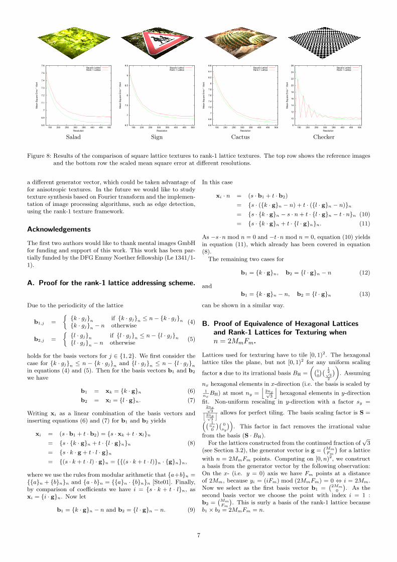
texture elements. Figure 8 shows the results of the numericalcomparison. Except for the checker board texture, rank-1 lat-tice textures consistently outperform the square lattice texturesfor any resolution as expected due to the increased samplingefficiency. The checker board is the worst-case comparison formaximized minimum distance rank-1 lattice textures to squarelattices as the checker board itself can be perfectly representedby a square lattice. Nevertheless, the rank-1 lattice shows aconsistent behavior and outperforms the square lattice whenthe resampled resolution is not a divider of the source resolu-tion.

The addressing on rank-1 lattices is slightly more expensivethan the addressing of square lattice textures. In our renderingsystem the performance drop was about 5% for all tested scenes.Since these scenes contain only simple geometry and lightingcalculations the relative performance cost is even less when amore complex scene is rendered.

Using rank-1 lattices for texture storage non-axis alignedstructures are visually more pleasing when the textures aremagnified and due to the good isotropic properties of MMDrank-1 lattices the quality does not depend largely on the ori-entation of the basis vectors. Nevertheless the basis vectorsdefine the preferred directions for straight lines as in any lat-tice. For texture minification our numerical results clearly showthe improved sampling efficiency over regular lattices.

7. Conclusions and Future Work

We have presented a new image and texture representation,which easily can be integrated in ray tracing and real-time ren-dering systems. For that purpose we have introduced an ad-dressing scheme based on the lattice point indices, as apparentin the rank-1 lattice definition. Thereby the natural structureof rank-1 lattices is exploited. The periodicity of rank-1 latticeallows for a simple tiled image representation, with the numbern of lattice points per tile being independent of the originalimage resolution. Therefore n always can be chosen freely, ac-cording to the application need, as a prime number or a powerof 2 for example. Note that even though most of the exampleswere on square regions maximized minimum distance rank-1lattices can be constructed for any aspect ratio and thus usedfor non-square textures as well without changing any of thecomputations.

Thanks to a higher sampling efficiency rank-1 lattice imagesprovide a better image quality than images on the square lat-tice at same storage cost. In fact, the sampling efficiency ofmaximized minimum distance rank-1 lattices very closely ap-proximates the one of the hexagonal lattice. We showed thatfor a subset of the rank-1 lattices they are in fact equal to thehexagonal lattice for texturing.

Using the proposed addressing scheme neighboring latticepoints are not necessarily neighbors in the image array on disk,which can influence cache performance. In Section 5.4 we al-ready indicated beneficial choices of generator vectors, however,an investigation with respect to cache performance still needsto be performed.

While for general isotropic textures the rank-1 lattices out-perform the traditional square lattice, textures containingmostly vertical and horizontal lines can not be representedsmoothly. In this case the rendering system should allow fortraditional texturing. We have not yet investigated embeddedlattices that would allow for classical image pyramids. Thusour multiresolution textures need to be always computed fromthe full resolution source image.

As rank-1 lattices are not restricted to the isotropic spectrum,they are also able to catch anisotropic structures by choice of

6

6.8

6.9

7

7.1

7.2

7.3

7.4

7.5

7.6

150 200 250 300 350 400 450 500

Me

an

-Sq

ua

re E

rro

r *

10

e4

Resolution

Square LatticeRank-1 Lattice

6.5

7

7.5

8

8.5

9

9.5

150 200 250 300 350 400 450 500

Me

an

-Sq

ua

re E

rro

r *

10

e4

Resolution

Square LatticeRank-1 Lattice

6.6

6.8

7

7.2

7.4

7.6

7.8

8

8.2

8.4

8.6

150 200 250 300 350 400 450 500

Me

an

-Sq

ua

re E

rro

r *

10

e4

Resolution

Square LatticeRank-1 Lattice

8

10

12

14

16

18

20

22

24

26

150 200 250 300 350 400 450 500

Me

an

-Sq

ua

re E

rro

r *

10

e4

Resolution

Square LatticeRank-1 Lattice

Salad Sign Cactus Checker

Figure 8: Results of the comparison of square lattice textures to rank-1 lattice textures. The top row shows the reference imagesand the bottom row the scaled mean square error at different resolutions.

a different generator vector, which could be taken advantage offor anisotropic textures. In the future we would like to studytexture synthesis based on Fourier transform and the implemen-tation of image processing algorithms, such as edge detection,using the rank-1 texture framework.

Acknowledgements

The first two authors would like to thank mental images GmbHfor funding and support of this work. This work has been par-tially funded by the DFG Emmy Noether fellowship (Le 1341/1-1).

A. Proof for the rank-1 lattice addressing scheme.

Due to the periodicity of the lattice

b1,j =

{k · gj}n if {k · gj}n ≤ n− {k · gj}n

{k · gj}n − n otherwise(4)

b2,j =

{l · gj}n if {l · gj}n ≤ n− {l · gj}n

{l · gj}n − n otherwise(5)

holds for the basis vectors for j ∈ {1, 2}. We first consider thecase for {k · gj}n ≤ n − {k · gj}n and {l · gj}n ≤ n − {l · gj}n

in equations (4) and (5). Then for the basis vectors b1 and b2

we have

b1 = xk = {k · g}n (6)

b2 = xl = {l · g}n. (7)

Writing xi as a linear combination of the basis vectors andinserting equations (6) and (7) for b1 and b2 yields

xi = (s · b1 + t · b2) = {s · xk + t · xl}n

= {s · {k · g}n + t · {l · g}n}n (8)

= {s · k · g + t · l · g}n

= {(s · k + t · l) · g}n = {{(s · k + t · l)}n · {g}n}n,

where we use the rules from modular arithmetic that {a+b}n ={{a}n + {b}n}n and {a · b}n = {{a}n · {b}n}n [Ste01]. Finally,by comparison of coefficients we have i = {s · k + t · l}n, asxi = {i · g}n. Now let

b1 = {k · g}n − n and b2 = {l · g}n − n. (9)

In this case

xi · n = (s · b1 + t · b2)

= {s · ({k · g}n − n) + t · ({l · g}n − n)}n

= {s · {k · g}n − s · n + t · {l · g}n − t · n}n (10)

= {s · {k · g}n + t · {l · g}n}n. (11)

As −s ·n mod n = 0 and −t ·n mod n = 0, equation (10) yieldsin equation (11), which already has been covered in equation(8).

The remaining two cases for

b1 = {k · g}n, b2 = {l · g}n − n (12)

and

b1 = {k · g}n − n, b2 = {l · g}n (13)

can be shown in a similar way.

B. Proof of Equivalence of Hexagonal Latticesand Rank-1 Lattices for Texturing whenn = 2MmFm.

Lattices used for texturing have to tile [0, 1)2. The hexagonallattice tiles the plane, but not [0, 1)2 for any uniform scaling

factor s due to its irrational basis BH =

„`10

´` 12√3

2

´«. Assuming

nx hexagonal elements in x-direction (i.e. the basis is scaled by1

nxBH) at most ny =

j2nx√

3

khexagonal elements in y-direction

fit. Non-uniform rescaling in y-direction with a factor sy =2nx√

3j2nx√

3

k allows for perfect tiling. The basis scaling factor is S =“` 1nx0

´`0

sy

´”. This factor in fact removes the irrational value

from the basis (S ·BH).

For the lattices constructed from the continued fraction of√

3(see Section 3.2), the generator vector is g =

`MmFm

´for a lattice

with n = 2MmFm points. Computing on [0, n)2, we constructa basis from the generator vector by the following observation:On the x- (i.e. y = 0) axis we have Fm points at a distanceof 2Mm, because yi = (iFm) mod (2MmFm) = 0 ⇔ i = 2Mm.Now we select as the first basis vector b1 =

`2Mm

0

´. As the

second basis vector we choose the point with index i = 1 :b2 =

`MmFm

´. This is surly a basis of the rank-1 lattice because

b1 × b2 = 2MmFm = n.

7

This rank-1 lattice has a basis of the form BL = Sr

“`10

´` 121

´”,

with Sr =

„` 1nx0

´`01

ny

´«, and is equivalent to a hexagonal lattice

scaled to tile the square with nx = Fm and ny = 2Mm. This istrue for all lattices with n = 2FmMm.

References

[AG85] Afflerbach L., Grothe H.: Calculation ofMinkowski-reduced Lattice Bases. Computing 35,3-4 (1985), 269–276.

[CR97] Cools R., Reztsov A.: Different Quality Indexesfor Lattice Rules. J. Complex. 13, 2 (1997), 235–258.

[CSB87] Conway J., Sloane N., Bannai E.: Sphere-packings, Lattices, and Groups. Springer-VerlagNew York, Inc., 1987.

[Csb05] Csbfalvi B.: Prefiltered Gaussian reconstructionfor high-quality rendering of volumetric data sam-pled on a body-centered cubic grid. In IEEE Visu-alization (2005), IEEE Computer Society, p. 40.

[CVF08] Condat L., Van De Ville D., Forster-HeinleinB.: Reversible, fast, and high-quality grid conver-sions. IEEE Transactions on Image Processing 17,5 (May 2008), 679–693.

[DK08] Dammertz S., Keller A.: Image Synthesis byRank-1 Lattices. In Monte Carlo and Quasi-MonteCarlo Methods 2006, Keller A., Heinrich S., Nieder-reiter H., (Eds.). Springer, 2008, pp. 217–236.

[Edw07] Edwards D.: Practical Sampling for Ray-BasedRendering. PhD thesis, University of Utah, 2007.

[EVM08] Entezari A., Ville D. V. D., Moller T.: Prac-tical box splines for reconstruction on the body cen-tered cubic lattice. IEEE Transactions on Visualiza-tion and Computer Graphics 14, 2 (2008), 313–328.

[Hel85] Helfrich B.: Algorithms to construct Minkowski-reduced and Hermite-reduced lattice bases. Theor.Comput. Sci. 41, 2-3 (1985), 125–139.

[HW81] Hua L., Wang Y.: Applications of Number Theoryto Numerical Analysis. Springer-Verlag and SciencePress, Berlin-New York, and Beijing, 1981.

[Kan87] Kannan R.: Algorithmic Geometry of Numbers.Annual Reviews in Computer Science 2 (1987), 231–267.

[Kor59] Korobov N.: The Approximate Computation ofMultiple Integrals. Dokl. Akad. Nauk SSR 124(1959), 1207–1210 (in Russian).

[Llo82] Lloyd S.: Least Squares Quantization in PCM.IEEE Transactions on Information Theory 28, 2(1982), 129–137.

[Mar03] Martinet J.: Perfect Lattices in Euclidean Spaces.Springer-Verlag, 2003.

[MS05] Middleton L., Sivaswamy J.: Hexagonal ImageProcessing: A Practical Approach (Advances in Pat-tern Recognition). Springer-Verlag New York, Inc.,2005.

[Nie92] Niederreiter H.: Random Number Generationand Quasi-Monte Carlo Methods. SIAM, Philadel-phia, 1992.

[NM02] Neophytou N., Mueller K.: Space-time points:4d splatting on efficient grids. In VVS ’02: Proceed-ings of the 2002 IEEE symposium on Volume visu-alization and graphics (Piscataway, NJ, USA, 2002),IEEE Press, pp. 97–106.

[Pea90] Peachy D.: Texture On Demand. Pixar technicalmemo 07-06, Pixar, 1990.

[PM62] Petersen D. P., Middleton D.: Sampling andReconstruction of Wave-Number-Limited Functionsin N-Dimensional Euclidean Spaces. Informationand Control 5, 4 (1962), 279–323.

[Sie89] Siegel C.: Lectures on Geometry of Numbers.Springer-Verlag, 1989.

[SJ94] Sloan I., Joe S.: Lattice Methods for MultipleIntegration. Clarendon Press, Oxford, 1994.

[Ste01] Steger A.: Diskrete Strukturen (Band 1).Springer-Verlag, 2001.

[VVPL02] Van De Ville D., Van De Walle R., PhilipsW., Lemahieu I.: Image Resampling Between Or-thogonal and Hexagonal Lattices. In Proceedings ofthe 2002 IEEE International Conference on ImageProcessing (2002), vol. III, pp. 389–392.

8