Texture Regimes for Entropy-Based Multiscale Image Analysis · Texture Regimes for Entropy-Based Multiscale Image Analysis 3 them is that such critical structures (extrema and discontinuities)

Texture Regimes for Entropy-BasedMultiscale Image Analysis

Sylvain Boltz1,2, Frank Nielsen1, and Stefano Soatto2

1 Laboratoire d’Informatique, Ecole Polytechnique, 91128 Palaiseau Cedex, France;boltz,[email protected]

2 UCLA Vision Lab, University of California, Los Angeles; Los Angeles – CA, 90095;[email protected]

Abstract. We present an approach to multiscale image analysis. Ithinges on an operative definition of texture that involves a “small re-gion”, where some (unknown) statistic is aggregated, and a “large region”within which it is stationary. At each point, multiple small and large re-gions co-exist at multiple scales, as image structures are pooled by thescaling and quantization process to form “textures” and then transitionsbetween textures define again “structures.” We present a technique tolearn and agglomerate sparse bases at multiple scales. To do so efficiently,we propose an analysis of cluster statistics after a clustering step is per-formed, and a new clustering method with linear-time performance. Inboth cases, we can infer all the “small” and “large” regions at multiplescale in one shot.

1 Introduction

Textures represent an important component of image analysis, which in turn isuseful to perform visual decision tasks – such as detection, localization, recogni-tion and categorization – efficiently by minimizing decision-time complexity [12].The goal of image analysis3 is to compute statistics (deterministic functions ofthe data) that are at the same time insensitive to nuisance factors (e.g., view-point, illumination, occlusions, quantization) and useful to the task (i.e., in thecontext of visual decision tasks, discriminative). Such statistics are often calledfeatures, or structures. Such structures have to satisfy a number of properties tobe useful, such as structural stability, commutativity, and proper sampling [12].The dual of such structures, in a sense made precise by Theorem 5 of [12], aretextures, or more precisely stochastic textures, defined by spatial stationarity ofsome (a-priori unknown) statistics. Regular textures, on the other hand, are de-fined by cyclo-stationarity (or stationarity with respect to a discrete group) ofsome (a-priori unknown) structure.

3 Image analysis refers to the process of “breaking down the image into pieces,” whichis prima facie un-necessary and even detrimental for data storage and transmissiontasks ([11], p. 88), but instead plays a critical role in visual decision tasks [12].

2 S.Boltz, F.Nielsen, and S.Soatto

Whether a region of an image is classified as texture or structure depends onscale.4 A region can be a structure at some scale, a texture at a coarser scale,then again a structure at yet a coarser scale and so on (Fig. 1), reflecting the lackof causality in two-dimensional scale-space [9]. Therefore, we do not seek for asingle transition from structure to texture [17, 18], but instead seek to representthe entire phase-space of transitions at each location in an image.

To address these issues, in Sect. 2 we introduce a definition of texture thatguides the development of efficient schemes for multiscale coding in Sect. 3, wherewe introduce an algorithm to compute statistics based on three fast clusteringalgorithms reviewed in Sect. 4.1 and 4.3, and a new variant introduced in Sect.4.2. These clustering algorithms allow us to perform multiscale analysis in oneshot (Sect. 5). The analysis can also be done directly in the clustering processwith linear complexity (Sect. 5.2).

Our characterization of textures uses three ingredients: A statistic, ψ, theminimal domain where such a statistic is pooled, ω, and the maximal domain(in the sense of inclusion) where it is stationary, Ω. Therefore, we focus ondefining suitable classes of statistics, and on designing efficient algorithms topartition the image into multiple regions. This is done through efficient tech-niques to create sparse bases (dictionaries), using clustering and dimensionalityreduction in high-dimensional non-Euclidean spaces. In particular, we introduce“kNN-Quick Shift,” a generalization of [16] modified to handle data distributedin high-dimensional spaces, and to allow different variables, such as scale, as“gap” measures. This enables simultaneous estimation of “small” ω and “big” Ωregions can be performed by alternating Min-Max entropy segmentation in lin-ear time. Our entropy measure exhibits a “staircase-like” behaviour, with eachstep determining the small regions ω at the lower edge, and the big regions atthe upper edge. Note that we achieve this in one-shot, for all scales, withouthaving to match patches or searching for periodic patterns [6].

2 Texture/Structure Multiple Transitions

Image structures are regions of the image that are salient (i.e., critical pointsof some functional, Def. 4 of [12]), repeatable (i.e., the functional is structurallystable, Def. 9 of [12]), and insensitive to nuisance factors (i.e., the functional isinvariant to group nuisances and commutes with respect to non-invertible ones,Def. 6 of [12]). For zero-dimensional structures (attributed points, or frames), ithas been shown that the attributed Reeb tree (ART) is a complete invariant withrespect to viewpoint and contrast away from occlusions [13]. However, occlusionsof viewpoint and illumination (cast shadows) yield one-dimensional structures,such as edges and ridges. The main technical and conceptual problem in encoding

4 Note that scaling alone is not what is critical here. Scaling is a group, so one canalways represent any orbit with a single canonical element. What is critical is thecomposition of scaling with quantization, which makes for a semi-group. Withoutquantization we would not need a notion of stochastic texture, since any regionwould reveal some structure at a sufficiently small scale.

Texture Regimes for Entropy-Based Multiscale Image Analysis 3

them is that such critical structures (extrema and discontinuities) are not definedin a digital image. For this reason, we must first define a notion of “discretecontinuity,” lest every pixel boundary is a structure. This is achieved by designinga detector, usually an operator defined on a scalable domain, and searching forits extrema at each location in the image, at each scale. In principle one wouldhave to store the response of such detectors at all possible scales. In practice,owing to the statistics of natural images, we can expect the detector functionalto have isolated critical loci that can be stored in lieu of the entire scale-space.In between critical scales, structures become part of aggregate statistics that wecall textures.

To make this more precise, we define a texture as a region Ω ⊂ D withinwhich some image statistic ψ, aggregated on a subset ω ⊂ Ω, is spatially station-ary.5 Thus a texture is defined by two (unknown) regions, small ω and big Ω, an(unknown) statistic ψω(I)

.= ψ(I(y), y ∈ ω), under the following conditions of

stationarity and non-triviality:

ψω(I(x+ v)) = ψω(I(x)), ∀ v | x ∈ ω ⇒ x+ v ∈ Ω (1)

Ω′\Ω 6= ∅ ⇒ ψΩ′(I) 6= ψΩ(I). (2)

The small region ω, that defines the intrinsic scale s = |ω| (the area of ω), is mini-mal in the sense of inclusion 6. Note that, by definition, ψω(I) = ψΩ(I). A texturesegmentation is thus defined, for every quantization scale s, as the solution of thefollowing optimization with respect to the unknowns ΩiNi=1, ωiNi=1, ψiNi=1

min

N(s)∑i=1

∫Ωi

d(ψωi(I(x)), ψi)dx+ Γ (Ωi, ωi) (3)

where Γ denotes a regularization functional and d denotes a distance, for instance`2, or a nonparametric divergence functional [2, 8].

In Sect. 3 we discuss the role of the statistics ψ. In Sect. 4, we discuss aboutsome clustering algorithms, introducing along the way a novel extension of aclustering algorithm that is suited for high-dimensional spaces. Finally we buildon these clustering algorithms to derive, in Sect. 5, two methods to automaticallycompute the set of all regions ωi and Ωi.

3 Multiscale Feature Selection and DictionaryAgglomeration

The difficulty in instantiating the definition of texture into an algorithm forimage analysis is that neither the regions ωi, Ωi, nor the statistics ψω are known

5 Constant-color regions are a particular (trivial) case of texture, where the statisticψ(I) = I is pooled on the pixel region ω = x. It is an unfortunate semanticcoincidence that such regions are sometimes colloquially referred to as “textureless.”

6 I(x), x ∈ ω is sometimes called a texton [7], or texture generator. This definitionapplies to both “periodic” or “stochastic” textures. Regions with homogeneous coloror gray-level are a particular case whereby ω is a pixel, and do not need separatetreatment.


Fig. 1. Left: multiple Texture/Structure Transitions: The same point can be inter-preted as either structure or texture depending on scale. Starting from a small redregion ω, the green region Ω determines the domain where some statistic computed inω is stationary (relative some group, which includes cyclo-stationarity when the groupis discrete).

a-priori. It is therefore common to define ψ in terms of a class of functions suchas a Gabor wavelets or other bases learned directly from the image under sparsityconstraints [1]. One can even consider just samples of the image in a windowof varying size around each pixel [15]. Whatever representation one chooses fora local neighborhood of the image at a given scale, the fact that all pointshave to be represented at all scales causes an explosion of complexity. This canbe mitigated by clustering the dictionary elements into a codebook, with eachdictionary element encoded with an index and representing a mode in the datadistribution. Each image region is then then represented by an histogram of theseindices. In principle, one could take these to be our statistics ψ, and representstructures as locations where the label histogram is surrounded by different ones,and textures as locations where the label histogram is surrounded by similar ones.

However, the dictionaries thus learned are usually very large and cumbersometo work with. Therefore, one can reduce the dimensionality of the representationby reducing the number of atoms in the dictionary. However, in order to achievethe insensitivity to nuisance factors described in the previous section, cluster-ing cannot just be performed with respect to the standard `2 distance as theatoms may undergo deformations. Clustering with an histogram-based distanceis also ill-advised as the distributions of different classes have significant overlap.Kullback-Leibler’s divergence naturally adapts to the supports and the modes ofthe distributions, and is therefore a natural choice for divergence measure. Thefeature space is then chosen so as to discount nuisance variability.

We propose clustering in three different feature spaces to agglomerate patchesmodulo three different types of transformation (Fig. 2): First, we consider ψω

.=


I(x, y), x, y(x,y)∈ω to get rid of small translations. In this feature space onepays a small price to align two similar I(x, y) as long as their (x, y) distance issmall. Similarly, polar coordinates I(x, y), r, ε.θ, with a small weight ε on theangle, are insensitive to small rotations and with a small weight on the radiusI(x, y), ε.r, θ they are insensitive small scalings (Fig. 2).

Fig. 2. (left) Clustering with a ”bag-of-features” dictionary of 256 image patches.Patches identical modulo small feature / geometry deformations are now agglomer-ated to one exemplar texture patch. (right) Clustering on sparse representation ofimages with uncertainty on value and position: the three columns show the differentfeature spaces, and red arrow shows the direction along which neighbors are preferablysearched for. The distance on these feature spaces is the symmetric Kullback-Leiblerdivergence.

Now, the last step is the most critical, for it involves clustering in high-dimensional and highly non-Euclidean spaces (Fig. 2). We will describe our ap-proach in the next two sections.

4 Three fast clustering algorithms

In this section we use two existing clustering algorithm, Quick Shift (QS) andStatistical Region Merging (SRM), and introduce a novel one, “kNN QuickShift,” that adapts QS to high-dimensional data.7 The purpose is to show thatthe analysis that follows is not dependent on the particular algorithm to arriveat a clustering tree.

7 Those two families of algorithms were also recently combined in [4].


4.1 Mode seeking with Quick Shift

Quick Shift [16] is a modification of Medoid-Shift that retains its benefit ofoperating on non-Euclidean spaces and still converges in one iteration.

yi(1) = arg minj:P (j)>P (i)

Dij (4)

τ(i) = Diyi(1) (5)

Its main advantage is simplicity and speed. One clustering with Quick Shiftgives a full segmentation tree as all nodes are connected to each other with adifferent strength τ called the gap. Thresholding this gap with different valuesthus yields different segmentations. The most common use of these clusteringalgorithms is with the feature space I(x), x, y, yielding compact regions ofuniform luminance or color usually called superpixels. In practice, the full matrixDij does not needed to be built, as the feature space often has a geometriccomponent, so physical neighbors are also neighbors in feature space. This limitsthe search to a small local window. Even if no geometric prior is available,one can still use a window of a certain size h around each datum. When thedata distribution is high-dimensional and sparsely distributed, a large h has tobe selected, leading to oversmoothing the estimate of the probability densityfunction (PDF), and to a computationally intensive search. In the next sectionwe introduce a modification of this algorithm designed to mitigate this problem,similarly to what [5] has done for Mean Shift.

4.2 kNN Quick Shift

To extend QS to high-dimensional data spaces we replace the Parzen densityestimator with a balloon estimator. The analysis of [14] shows that, althoughbaloon estimators underperform Parzen in one dimension, they improve as thedimension of the space increases. We choose the neighborhood of possible con-nections to be the k-nearest neighbors Nk(i) of each point.

yi(1) = arg minj:j∈Nk(i)&Pj>Pi

Dij (6)

The resulting kNN Quick Shift is made very fast by using approximate nearestneighbors with (1 + ε) tolerance. In practice, this works well if k is low, sowe implemented a recursive kNN-Quick Shift algorithm: It first builds a treeconnecting pixel values, then unconnected superpixels are connected until everynode is linked.

When clustering pixels in an image, Dij is simply the Euclidean distancebetween two pixel features. When clustering patches for agglomeration of basesmodulo some deformations, Dij is the symmetric Kullback-Leibler divergencecomputed on three different feature spaces (Sec. 3). The parameter k exertsdirect control on the cluster size. It can therefore be used as a gap measure toperform a cut of the tree structure provided by QS. This is particularly relevantin the context of texture analysis, where we seek the smallest ω and largest Ωregions where certain statistics are stationary. However, it is inconsistent with aregion based energy as defined in eq. (3).


4.3 A fast statistical region merging (SRM)

SRM is an efficient greedy algorithm [10] for region merging with theoreticalguarantees. Every pair of adjacent pixels (both horizontally and vertically) isassigned a strength value, for instance the absolute value of their intensity dif-ference. The list is then sorted, and location labels retained. For each pair ofpixels, a test called predicate is run to decide if the regions are to be merged.This runs in linear time as it only goes through all the pixel pairs once (2N -complexity). The region merging structure is a union find data structure whichallows finding pixel labels with complexity O(1). In order to build a segmentationtree with this algorithm, the predicate is made to depend on a scalar parameter,and the same algorithm is run repeatedly for increasing values of the parameterand with pairs of adjacent regions instead of pairs of pixels.

5 Recursive Max-Min Entropy for Texture Analysis

From the operational definition of texture (2), we seek to efficiently computea multiscale representation to simultaneously detect the small ω and large Ω.The basic intuition comes from the observation that aggregating adjacent su-perpixels yields an increase in the entropy of the aggregate descriptor, up to thepoint where a minimum stationary region is reached, ω. At that point, aggre-gating further regions will not change the entropy, because of the stationarityassumption (of course, the complexity of the encoding will decrease, as more andmore superpixels are lumped into the same region), up to the point where theboundary of the large region Ω is reached. Aggregating superpixels outside thisregion will cause the entropy to resume its climb.

The recursive fucntional reads, initializing ω(0)i as N different regions of 1

pixel size, where N is the number of pixels in the image,Ω

(k)i = arg min

Ωi

N(s)∑i=1

∫Ωi

H(ψω

(k)i

(I(x)))dx+ Γ (Ωi)

ω(k)i = arg max

ωi

N(s)∑i=1

∫ωi

H(ψΩ

(k−1)i

(I(x)))dx− Γ (ωi)

(7)

where H is the Shannon entropy.We propose two methods to perform this optimization. Building from a seg-

mentation trees e.g. Sec. 4.1, 4.2, or 4.3 Method 1 performs a constrained opti-mization as a line search in the tree of superpixels. While Method 2 is a free-formoptimization in the image domain.

5.1 Method 1 : Constrained solution from a pre-processedsegmentation tree

To instantiate this, we use the entropy-based saliency function introduced in [8],followed by entropy-based segmentation, as customary [2].


Using the dictionary features defined in Sect. 3, and the superpixel segmen-tation map at a given scale, one can compute an entropy H of features insidethe superpixel containing i:

Hi(s) = −D∑x=1

Pi(x, s) logPi(x, s) (8)

where Pi is the distribution of the reduced dictionary features built on the regiondefined by i, i.e., the superpixel S(i, s), D is the size of the dictionary,

Pi(x) =1

|S(i, s)|∑

p∈S(i,s)

δ(x− d(p)) (9)

and δ is Dirac’s delta, d(p) is the index of the dictionary at point p. The smallscale of a texture is defined as the largest scale at which entropy stops increasing:

ω(i, s) = S(i, s′)

s′ = arg maxt>st | ∀v s ≤ v ≤ t, dHi(v)ds > 0. (10)

The stationary domain of the texture Ω is simply defined as the boundary ofthe region past which entropy resumes increasing,

Ω(i, s) = S(i, s′′)

s′′ = arg maxt>st | ∀v s ≤ v ≤ t, dHi(v)ds ≤ 0 (11)

Therefore, we perform the final segmentation at the maximum region that pre-serves stationarity.

While this method can be used with any segmentation tree, the solutionwill be constrained as unions of preprocessed segmentations. An unconstrainedfree-form solution can be found by building a segmentation tree that optimizesdirectly a Min-Max entropy in linear time using the properties of SRM.

5.2 Method 2 : SRM with alternate Min-Max entropies

We start from an initial segmentation ωi, e.g., from SRM, to initialize the statis-tics, then perform SRM again with the ordering of neighboring segments givenby sorting the strength between segments Γ =

∫∂Ωi‖∇I(x)‖2 dx in increasing

order. Now the predicate changes to an entropy-increasing or -decreasing test,and regions are merged only if entropy keeps decreasing or is constant. Once aregion Ωi is found, we turn to maximizing the entropy to find the region ωi. Theordering of Γ neighboring segment is now sorted by decreasing order, and theregions are merged if entropy increases. In this way, one can define an alternat-ing Min-Max entropy exploration of the image with the same complexity, sincethe neighboring graphs are only processed once. The number of merging tests isagain linear in the number of pixels in the image.


5.3 Features Persistence and stability

If the hypothesis underlying our definition of texture is correct, entropy willhave a staircase-like behavior, with flat plateaus bounded below (in the senseof inclusion) by the small region ω, and above by Ω. As the same region canswitch back-and-forth from texture to structure, we expect several such plateausas the scale of inclusion changes. In the next section, we verify this hypothesisempirically on different superpixels from natural images. While this behavior isgiven a priori in the Min-Max entropy clustering, it is not obvious that it willbe manifest when using any segmentation tree.

Those entropy profiles at each pixel are now agglomerated into one globalhistogram of entropies using a voting approach. As a staircase value of entropyappears at one pixel, it sums as a weighted contribution in the histogram ofentropies, the weight being simply the length of the step. This histogram thusshows the different stable regimes of entropies appearing in the image. Knowingthis histogram, one can deduce simply the local scale at a pixel position by doingmode seeking on this histogram (smoothed as a PDF). The definition of a localscale at one pixel position is the smallest scale where a mode value of the globalhistogram entropy appears. This allow us to perform stable segmentation anddescription of the natural scale of the image at a pixel, according to a structuralstability criterion where the length of each step measures the structural stabilitymargin [12].

6 Experimental results

6.1 Computational speed

In this section we explore the complexity and performance of the one dictionarylearning and four clustering algorithms discussed. Computational speed is shownin Table 1, measured in seconds on a matlab/C implementation. Three differentmethods are used to build the dictionaries : (1) Color dictionary using k-means(2) Texture dictionary using k-means (3) Texture dictionary using k-means andagglomerated using a QS with Kullback-Leibler divergence. Based on those threedifferent features, four different segmentation trees have been built: (a) ClassicalQS as described in Sect. 4.1 (b) kNN QS , with a scale parameter, designed forhigh dimensional spaces in Sect. 4.2 (c) Classical SRM as described in Sect. 4.3(d) SRM with alternated min max entropies as described in Sect. 5.2

Method (1) (2) (3) (a) (b) (c) (d)

Speed 0.2 4.1 8.1 0.4 0.1 1.5 3.8

Table 1. Running times in seconds, (1,2,3) dictionary learning methods (a,b,c,d) seg-mentation tree methods


6.2 Dictionary agglomeration

We illustrate agglomeration by clustering a dictionary built on the “Barbara”image to eliminate nuisance variations such as small rotations, translations, andcontrast changes. QS does not require a smooth embedding, so it can be used witha non-Euclidean metric, for instance one defined on the quotient space under thenuisance group. We use the symmetrized Kullback-Leibler divergence estimatedwith an efficient kNN-based estimator [3]. For every atom we build the pairwisedistance matrix Dij in (6). The first stage, with feature space I(x, y), x, y,forms a big cluster containing most of the texture elements “stripes” (Fig. 2).This dictionary now contains only one atom representing this texture cluster, or“exemplar.”

In order to evaluate the efficiency of this agglomeration we take 32 randomimages from the Berkeley segmentation dataset. For each one we compare fourways of building a 128-atom dictionary: (i) direct k-means on the patches, (ii)first learning 256 clusters, then reducing QS using either `2, or (iii) KL clusteringon I(x, y), and finally (iv) KL clustering on I(x, y), x, y. One measure ofefficiency of these dictionaries is the spatial coherence of the index of the atomsused. To measure it, one can compute first a color segmentation (in order to beindependent of the texture measures) on each image and sum the entropies ofeach segment. The lower this entropy Haverage, the more coherent the index ofthe atoms.

Haverage(feature) =1

32

32∑i=1

1

NS(i)

NS(i)∑s=1

H(feature)(i, s) (12)

whereNS(i) is the number of superpixels in image i across all scales,H(feature)(i, s)is the entropy of a given feature, in image i, inside superpixel s. In this sectionthe feature used is the index of the dictionary. Average entropies shown in Tablereveal that one can obtain coherent sparse decompositions in natural images andthus efficient dimensionality reduction.

(a) (b) (c) (d)

Haverage(index) 3.25 3.10 3.17 2.21Table 2. Agglomeration of dictionaries for efficient sparse representation. Sum of en-tropies over all the superpixels. (a) k-means on 128 elements, (b) (c) (d) k-meanswith an initial size of 256 reduced to 128 with, (b) `2 clustering, (c) KL clustering onI(x, y) (d) KL clustering on I(x, y), x, y.

This method is also computationally tractable as it runs on the space of bases,rather than the space of all image patches as in [2]. However, as the scale ofthe texture is unknown, it can contain many dictionary elements. A solution isto look for the dictionary dimension that gives uniform regions in the space of


coefficients. Another solution is to try to find the natural scale of the texturesusing region growing algorithms, in our case superpixels aggregating across thetree of possible segmentations.

6.3 Multiscale region analysis

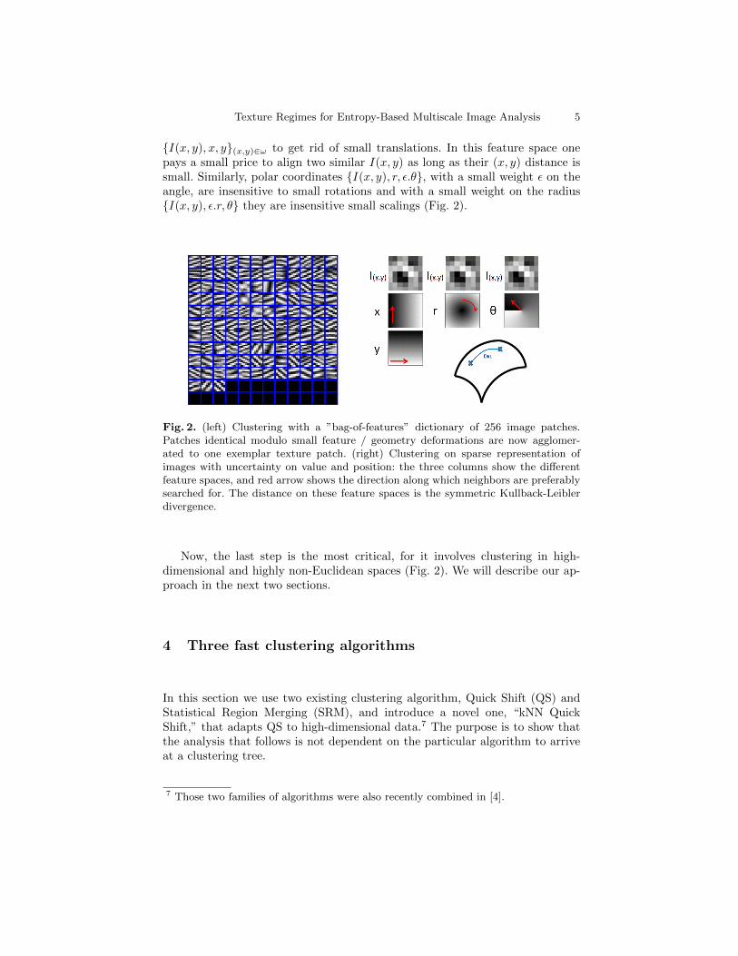
An illustration of the multiscale region analysis is shown in Figure 3. From one

Fig. 3. It shows the entropy regime of 6 randomly selected points in the first image, bygoing through the different scales of the segmentation tree. Staircase is visible and showsthe successive entropy regime of superpixels from successive ω regions to Ω regions.The regions are computed with QS trees. Detection of critical scales of textures on twodifferent images. The segmentation scheme is now SRM Min-Max.

image, a superpixel map is computed at different scales. Then the dictionaryfeatures are computed and agglomerated. Finally, for six randomly select pointsinside each superpixel, we plot the variations of entropy. It is evident that, asscale increase, entropy increases in steps. The stationary regime corresponds withsuperpixels merging with others of similar distribution. Structural transitionsoccur when superpixels merge that have different distributions. The process endswhen no new regions are discovered. These phase changes serve to detect ωi andΩi, which are displayed for different superpixels at key scales when the entropyregime changes. In Figure 4, critical scales at successive levels are shown. Firston a synthetic image, starting from one pixel, critical scales are: the pixel itself,the dark brown region minimizing entropy, then maximizing entropy, the lightbrown region to form an ”L” , then minimizing entropy again, until the entireimage is segmented. The same process is shown for a natural image; a light brickis first selected, then agglomerated with a darker one, then with a window, thenwith the whole building since all the statistics that describe the building arecaptured.

6.4 Scale Segmentation

The natural scale of a pixel is then extracted as described in Sect. 5.3. We usethe segmentation tree SRM Min-Max with the features based on agglomerated


dictionaries. Once the critical scales are computed, one builds a PDF of entropiesover all superpixels. The scale at one pixel is defined as the smallest scale atwhich a mode appears. Those modes show stable regimes of entropies and canbe used as a feature for scale segmentation. They also have the property of beingaccurate at boundaries, since the size of statistics is adaptive.

Fig. 4. Scale segmentation results on two images. By computing the statistics at theright scale, one can segment boundaries with pin-point precision, rather than sufferingfrom “fat-boundary effects” common in texture segmentation. Last image shows aresult with a standard texture segmentation algorithm [6] suffering from uniform scaleselection and “fat-boundary effects”

6.5 Stability

To evaluate stability, again thirty-two images of the Berkeley segmentationdataset are again randomly selected. If the critical scales extracted are correct,there should be some coherence in all the regions extracted across the image(since our definition does not leverage on any matching, this condition is notforced by construction). The measure of stability is then the average entropyover the 32 images over all the superpixels as described in Sect. 6.2 and Equa-tion (12). The features used here are size and color of the superpixels. Suchfeatures, if regions are stable and consistent, should have a low entropy acrossthe image. That means that many regions should be similar in size and color innatural images.

7 Discussion

We have presented an approach to multiscale texture analysis. The operativedefinition of texture we introduce guides the development of algorithms thatefficiently enable the estimation of all the “small regions” (a.k.a. “texton re-gions”), the “big regions” (a.k.a. “texture segments”) and the statistics within.We have introduced a novel clustering algorithm adapted for high-dimensionalspaces, and showed how an information-theoretic criterion can be used to definethe “gaps” to simultaneously detect small and large regions.


(a-1) (a-2) (a-3) (b-1) (b-2) (b-3)

Haverage(color) 3.17 3.01 2.88 3.08 2.97 2.81

Haverage(size) 4.87 4.52 4.18 4.15 4.12 4.05

(c-1) (c-2) (c-3) (d-1) (d-2) (d-3)

Haverage(color) 3.11 3.01 2.95 2.22 2.14 2.07

Haverage(size) 4.51 4.21 4.12 4.17 4.08 3.98

Table 3. Stability of critical scales extracted using four different segmentation trees(a,b,c,d) based on three different features (1,2,3). The dictionaries, all of size 128, are:(1) Color (2) Texture (3) Agglomerated Texture using QS with Kullback-Leibler asdescribed in Sect. 3. The segmentation trees are (a) QS described in Sect. 4.1 (b) kNNQS described in Sect. 4.2 (c) SRM described in Sect. 4.3 (d) SRM Min-Max entropydescribed in Sect. 5.2. The best result for each features and entropy (color or size of thecritical scales) is shown in bold. The best overall result is obtained with SRM Min-Maxwith agglomerated texture dictionary features.

Acknowledgment

Research supported by ONR N00014-08-1-0414 and ARO 56765-CI.

References

1. M. Aharon, M. Elad, , and A.M. Bruckstein. The k-svd: An algorithm for design-ing of overcomplete dictionaries for sparse representation. IEEE Transactions OnSignal Processing, 54(11):4311–4322, Nov 2006.

2. S.P. Awate, T. Tasdizen, and R.T. Whitaker. Unsupervised texture segmentationwith nonparametric neighborhood statistics. In European Conference on ComputerVision, pages 494–507, Graz, Austria, 2006.

3. S. Boltz, E. Debreuve, and M. Barlaud. High-dimensional statistical distance forregion-of-interest tracking: Application to combining a soft geometric constraintwith radiometry. In IEEE International Conference on Computer Vision and Pat-tern Recognition, Minneapolis, USA, 2007.

4. F. Chazal, L. J. Guibas, S. Y. Oudot, and P. Skraba. Persistence-based clusteringin Riemannian manifolds. Research Report 6968, INRIA, June 2009.

5. Bogdan Georgescu, Ilan Shimshoni, and Peter Meer. Mean shift based cluster-ing in high dimensions: A texture classification example. In IEEE InternationalConference on Computer Vision, page 456, 2003.

6. B. W. Hong, S. Soatto, K. Ni, and T. F. Chan. The scale of a texture and its ap-plication to segmentation. In IEEE International Conference on Computer Visionand Pattern Recognition, 2008.

7. B. Julesz. Textons, the elements of texture perception and their interactions.Nature, 1981.

8. T. Kadir, A. Zisserman, and M. Brady. An affine invariant salient region detector.In European Conference on Computer Vision, 2004.

9. T. Lindeberg. Scale-space theory in computer vision. Kluwer Academic, 1994.10. Richard Nock and Frank Nielsen. Statistical region merging. IEEE Transactions

Pattern Analysis Machine Intelligence, 26(11):1452–1458, 2004.


11. C. P. Robert. The Bayesian Choice. Springer Verlag, New York, 2001.12. S. Soatto. Towards a mathematical theory of visual information. (preprint) 2010.13. G. Sundaramoorthi, P. Petersen, V. S. Varadarajan, and S. Soatto. On the set

of images modulo viewpoint and contrast changes. In Proceedings of the IEEEConference on Computer Vision and Pattern Recognition, June 2009.

14. G. R. Terrell and D. W. Scott. Variable kernel density estimation. The Annals ofStatistics, 20:1236–1265, 1992.

15. M. Varma and A. Zisserman. A statistical approach to material classification usingimage patch exemplars. IEEE Transactions Pattern Analysis Machine Intelligence,to appear.

16. A. Vedaldi and S. Soatto. Quick shift and kernel methods for mode seeking. InEuropean Conference on Computer Vision, volume IV, pages 705–718, 2008.

17. Y. N. Wu, C. Guo, and S. C. Zhu. Perceptual scaling. Applied Bayesian Modelingand Causal Inference from an Incomplete Data Perspective, 2004.

18. S. C. Zhu, Y. N. Wu, and D. Mumford. Minimax entropy principle and its appli-cation to texture modeling. Neural Computation, 9:1627–1660, 1997.

Documents

Texture Regimes for Entropy-Based Multiscale Image Analysis · Texture Regimes for Entropy-Based Multiscale Image Analysis 3 them is that such critical structures (extrema and discontinuities)