Embed Size (px)
Citation preview

ISSN 1519-4612
Universidade Federal Fluminense
TEXTOS PARA DISCUSSÃO
UFF/ECONOMIA
Universidade Federal Fluminense
Faculdade de Economia
Rua Tiradentes, 17 - Ingá - Niterói (RJ)
Tel.: (0xx21) 2629-9699 Fax: (0xx21) 2629-9700
http://www.proac.uff.br/econ/graduacao
Editor: Luiz Fernando Cerqueira; [email protected]; [email protected].
*BNDES, E-mail: [email protected]
**BNDES, E-mail: [email protected]
***Professor Adjunto da Faculdade de Economia/UFF, E-mail: [email protected].
****BNDES, E-mail: [email protected]
Credit scarcity in developing countries: an
empirical investigation using Brazilian firm-
level data
André Albuquerque de Sant’Anna*
Antônio Marcos Hoelz Pinto Ambrozio**
Filipe Lage de Sousa***
João Paulo Martin Faleiros****
TD 305 Março/2015
Economia – Texto para Discussão – 305
2
Abstract
The aim of this paper is investigating whether Brazilian industrial firms are
credit constraint. We exploit a rich database that contains more than 3.000
firms with characteristics that may affect their degree of credit constraints:
size, being listed in the Brazilian stock market and level of exports-sales ratio.
Our results show that all dimensions considered here may affect the
sensitiveness of investment to cash flow, i.e., large firms, stock market listed
companies as well as large export capacity are associated with inexistence or
less credit restriction. Specifically, considering firm’s size, our results
corroborate the economic theory prediction and empirical international
literature. However, when compared to Brazilian studies, our findings are
similar to Terra (2003), however, they differ from Aldrighi and Bisinha (2010)
evidences that are based only on listed firms. Furthermore, the influence of
being listed in the stock market and export capacity is beyond any possible
correlation with size. Even small and middle firms are not credit constraint
when listed in the stock market or when the exports-sales ratio is higher.
Resumo
O objetivo desse artigo é investigar se as empresas industriais brasileiras sao
restritas ao crédito. Nós exploramos uma rica base de dados com mais de 3
mil empresas com características que podem afetar o seu grau de restrição de
crédito: tamanho, listada na BOVESPA e seu nível de exportação (medido pela
razão entre exportação e vendas). Nossos resultados mostram que todas as
dimensões consideradas nesse artigo podem afetar a sensibilidade do
investimento ao seu fluxo de caixa, isto é, grandes empresas, empresas
listadas na BOVESPA e exportadoras estão associadas a uma menor restrição
de crédito. Especificamente, considerando o tamanho da empresa, nossos
resultados corroboram a previsão dos artigos teóricos em empíricos da
literatura internacional. Entretanto, quando comparado com outros estudos
sobre o Brasil, nossos resultados são semelhantes aos de Terra (2003), porém
diferem das evidências de Aldrighi e Bisinha (2010), os quais são baseados em
empresas listadas na BOVESPA. Adicionalmente, a influência de estar listada no
mercado de capitais e a capacidade exportadora não está correlacionada com o
tamanho. Mesmo empresas pequenas e médias não são restritas ao crédito
quando listadas no mercado de capitais or quando a relação entre exportação
e vendas é alto.
Keywords: Credit Constraint, Firm’s Investment, Cash Flow, Exports, Stock
Market.
JEL Classification Code: D92, E22
Economia – Texto para Discussão – 305
3
1. INTRODUCTION1
Credit constraint is a widespread market failure, especially in developing countries, as
evidenced by Banerjee and Duflo (2005). Its adverse consequences, inhibiting
entrepreneur capacity to make investments, are particularly important to these countries,
which needs to accumulate capital and implement innovations to accelerate growth.
This paper investigates whether Brazilian companies are credit constrained
considering the investment-cash flow model proposed by Fazzari, Hubbard and Petersen
(FHP, 1988). The main interest in this case is to verify the sensitiveness of firm’s
investment to cash flow as synonyms of credit constraint. The use of a large and yet few
exploited dataset is one of the main contribution of the paper. It contains balance sheet
information for more than 3,000 industrial firms with characteristics that may affect the
degree of credit constraints, for example, size, the participation in the Brazilian stock
market and level of export’s sales.
Despite heterogeneity in our sample, the presence of non-listed firms imposes some
difficulties. In particular, Tobin’s Q can not be used as a proxy for investments
opportunities. This problem is circumvented by using multiple alternative proxies. For
instance, we consider variation of sales at firm level and sector variation in investment
and in value added at an aggregate level in order to control for investment opportunities.
Our main results indicate that Brazilian firms were credit constrained in recent years
(2008-2010). Cash flow coefficient is indeed larger than what is usually obtained in the
literature for other countries, such as Carpenter and Guariglia (2008), suggesting a
higher degree of imperfections in the Brazilian credit market. Furthermore, this
coefficient changes when firms are classified according to the three categories that may
properly approximate the degree of credit constraint: size, listed on stock markets and
the export’s sales level. In the first case, Brazilian firms are classified as small, middle
and large considering the number of employees. Although previous evidence that
analyses the impact of size on credit restrictions has been mixed in Brazil, as observed
in Terra (2003) and Aldrighi and Bisinha (2010), our results are in line with the
traditional literature: cash flow coefficient is insignificant or at least (depending on the
econometric specification) has a lower elasticity magnitude for larger firms.
Our two other categories, companies listed on the Brazilian stock market (public
versus non-public firms) and level of export to sales ratio (no export at all, below and
above the median) provide evidence that investments for firms listed in stock markets
and for those large exporters are not sensitive to cash flow variation. Besides, the
influence of these categories is beyond any possible correlation with size. When
interacting those dummies, listed and export, with size groups, our results suggest that
while no-large firms are in general credit constrained, this credit restriction was
softened for listed firms and large exporters. In this context, understanding stock market
participation as a “domestic” source of external investment’s funds and the level of
export’s sales as a proxy for “foreign” source, once export revenue may be seen as a
collateral to get access to international financing, our results suggest that these firms’
characteristics are effective to evaluate their degree of credit restrictions.2
In order to perform our investigation, this paper is structured in 5 sections apart from
this introduction. Section 2 provides a brief survey of the literature. Section 3 presents
1 We acknowledge financial support from Brazilian Development Bank (BNDES). The views expressed herein
are those of the authors and do not necessarily reflect the views of the Brazilian Development Bank. 2 Some care is necessary to deal with potential selection problems. It is possible that the whole process
needed to go public or to export, especially the requisites of transparency, is what is relevant to suppress
credit constraints.

Economia – Texto para Discussão – 305
4
methodology to analyze credit restriction. Data description is presented in Section 4 as
well as some descriptive statistics on the main variables. Next, we present and discuss
our results, followed by robustness outcomes. Last section concludes.
2. RELATION TO THE LITERATURE AND THE BRAZILIAN
CONTEXT
In a world of perfect capital markets, without transaction costs and taxes, the
Modigliani-Miller Theorem asserts that financial structure of firms are irrelevant for
their real decisions, in particular investments. But in reality all these assumptions are
non-valid, and a special focus of the literature has been the case of asymmetric
information. The asymmetries in financial markets may be due to differential
information about types, where borrowers have more information about their projects
risks or managerial abilities than creditors, or due to difficult verifiability of actions,
where creditors cannot observe investment choices or the real capacity of repayment
from borrowers. The main consequence is a gap between the internal (for example,
retained profits) and external (for example, bank credit) cost of funds, explained by the
creditor need to raise funds to compensate risk of bad quality borrowers (the adverse
selection problem) or costly monitoring (the moral hazard problem) (Stiglitz and Weiss,
1981).
An empirical testable implication of higher costs from external sources is that
increases in firm`s cash flow must push more investment. Moreover, as supposed by
major part of the literature, another implication should be a more sensitive correlation
between cash flow and investment in firms where information costs (and hence the gap
between the internal and external costs of funds) are higher.
The seminal researchers testing these hypotheses were Fazzari, Hubbard and Petersen
(FHP, 1988). They split a sample of US firms in three categories regarding dividend
payments, high, medium and low, and showed that the relation between cash flows and
investments were significantly higher in the last group, which corroborates the
hypothesis when one assumes that these kind of firms are more likely to suffer credit
restrictions.
This paper lead to an extensive empirical literature, where two main themes have been
emphasized: the need to control in an appropriate manner for investment opportunities,
where otherwise a positive association between cash flow and investment may simply
say that better opportunities induce firms investment and at the same time impact cash
today, and a critic of the basic methodology employed in FHP regarding the criteria for
splitting the firms in different classes of information costs.
Concerning the first problem, the initial proxy used for controlling investment
opportunities, Tobin`s Q, was criticized because what can be constructed using real data
(mean Q) is equivalent to what in theory reflect investments opportunities (marginal Q)
only under strong assumptions. Moreover, since Tobin`s Q, as the ratio between firm
market value and recomposition cost of capital, only reflects investment opportunities
from an outside point of view, which may not properly capture real opportunities under
imperfect capital markets (Carpenter and Guariglia, 2008). Besides, this proxy is simply
absent when one analyses data with non-traded firms (Baum et al., 2011; Guariglia et
al., 2011).
The response to this problem has been mixed in the literature, ranging from the
development of alternative proxies that can better capture investment opportunities to a
change in methodology that abandons the necessity of using Tobin’s Q. For the first
approach, prospect of future expense in capital goods is used to complement

Economia – Texto para Discussão – 305
5
information in Tobin’s Q in order to capture the internal view of opportunities
(Carpenter and Guariglia, 2008), or more aggregate variables are used in this regard, as
industry-level value-added growth when data base contains firms not traded publicly
(Guariglia, Liu e Song, 2011). For the second, it is better exemplified by the “Euler
equation approach” to the problem, where one tests if the firms’ investment behavior is
consistent with the first-order condition that may prevail when they solve a dynamic
programming problem under perfect markets (Bond and Meghir, 1994). Although many
of these proposed solutions may be ingenious, the fact is that it is really very hard to do
a proper control. Most studies are subject to the critic that a statistically positive
correlation between cash flow and investment may reflect mis-measured investment
opportunities.
Another challenge to this literature is given by how to classify firms regarding to
levels of information costs. In an influential paper, Kaplan and Zingales (KZ, 1997)
argued that theoretically the relation between the dependence of investments to internal
funds and information costs was not necessarily monotonic. They reviewed the seminal
article of FHP, and splitting their low dividend payment sample with respect to the
probability of liquidity need, they showed that in firms more propense to be short of
liquidity, the relation between cash flow and investment was weaker, contrary to the
original hypothesis sustained by FHP. Moreover, an interesting insight raised by KZ is
that it is difficult to say if this result is at odds with the literature so far, because in many
known papers the financial criteria used to classify firms between more or less credit
restricted may not correspond to the real information costs and hence effective credit
constraint of this firms: for instance, firms linked to a bank (conglomerates) may be less
credit constrained under an adverse selection story where the “lemons risk” limits
access to capital markets, but otherwise may be more financially dependent under a
story of monopsonic power of incumbent creditor.
KZ paper was the origin of a huge controversy in this literature, with some authors
reaffirming KZ findings (Clearly, 1999) while others criticizing their approach (for
instance, Hubbard 1998 or Allayannis and Mozumdar, 2004). One of the main
arguments against KZ is that firms classified as most prone to suffer illiquidity are in
general financially distressed, where creditors may seize their new generated funds as
repayment for old debts weakening in this way the relationship cash flow – investment.
Beyond this controversy, a point that must warm researchers refers to the properly
classification of firms by categories that really measure information costs. In fact,
Cleary (2007) arguments that the sensitivity of cash flow – investment between firms
with more or less financial restriction depends crucially on what variables are used to
classify firms as credit constrained.
The relation between investment and cash-flow was also studied in Brazil. In fact, the
structure of Brazilian capital markets is suggestive that firms may be subject to credit
constraints. While the banking system is considered robust and sophisticated, the
segment of long term credit is a point of weakness, being covered almost exclusively by
state-owned institutions. The market for corporate bonds is incipient, due, for instance,
to the difficult of developing a secondary market that may provide liquidity for potential
investors. On the other hand, stock market is relatively well developed, but only a few
firms have access to it.
Terra (2003) is one of the main references in the Brazilian literature. More recently,
we can cite the work of Aldrighi and Bisinha (2010). The general conclusion of these
authors is that Brazilian firms are indeed credit-constrained. However, in odds with the
conventional literature, firms that should be more credit constrained when using some
standard measure (size, for instance) do not appear to have a more significant

Economia – Texto para Discussão – 305
6
coefficient in the investment – cash flow equation. In Terra (2003), the hypothesis that
the cash flow coefficient is equal for large and small firms cannot be rejected, unless in
a limited period of time (1994-1997) when credit constraints were softer among large
firms3. In Aldrighi and Bisinha (2010), the cash flow coefficient is always significant,
and indeed increases with firm size. The authors suggest that financial difficulties
between firms with smaller size may explain their findings, as the desire to maintain a
“financial slack” avoiding in this way future liquidity problems may weaken the
investment – cash flow relationship.
A main feature of both papers is that they use information of firms which are required
by law to make their balance sheet data public, since their shares are available in the
stock market. As mentioned in the introduction, we contribute to this literature by
analyzing also firms not listed in the stock market, which correspond to the major part
of Brazilian firms. And for the two main concerns of the literature cited before, our
paper controls for investment opportunities using variables at the firm, as well as at the
sectorial level. Furthermore, regarding the classification of firms within different
information costs, we believe that the categories we use, size, access to capital markets,
and export capacity, can properly measure credit constraints.
3. METHODOLOGY
The model to investigate whether Brazilians firms are credit constrained is based on
Carpenter and Guariglia (2008) and Guariglia (2008), as shown in (1).
ititititititit XKFlowCashKI )/(/ 11 (1)
where i and t identify, respectively, firms and time, tI is the firm’s investment, tK is
the firm’s fixed asset, t is the time-effect for controlling business-cycle effects, i is
the fixed-effect, and it is the error-term. For robustness checks, the specification (1)
may include covariates itX , given by investment opportunities variables, that also
impact the dependent variable.
For eliminating firm-effect, we estimate equation (1) by fixed-effect and first-
difference. Time-effect is controlled by imposing dummies for instant t. Furthermore, to
control for industry-effect, another way to embody investment opportunities, we have
included dummies for each industry j interacted with time dummies in all estimated
models.
The OLS in first-difference may present the problem of endogeneity. Due to this fact,
we apply Generalized Method of Moments approach (GMM) based on Arelano and
Bover (1995) and Blundell and Bond (1998). This approach combines the standard set
of equations in first-difference with lagged levels of regressors as instruments, with the
incorporation of equations in levels with lagged first-difference as instruments.
The parameter of interest is ̂ . In the presence of imperfection in credit market, the
estimated coefficient ̂ should be positive and statistically significant, i.e., the firm’s
investment is sensitive to the cash flow, as discussed previously.
Although the main aim of the paper is to evaluate whether Brazilian manufacturing
firms are credit constraint, we also investigate whether there are differences in the cash
3 Indeed, the country experienced large inflows of FDI due to the privatization program in this period.

Economia – Texto para Discussão – 305
7
flow coefficient across the following groups of firms: (i) their size, evaluated by number
of employees; (ii) whether they are listed or not on the stock market; and (iii) the level
of firm’s exports, given by the ratio between exports and sales revenue. All these
classifications allow coefficients of control variables to differ across observations in the
distinct sub-samples and it will indicate the level of financial constraints faced by firms.
Thus, cash flow variable may be interacted with different dummies variables:
a) itSMALL refers to the firms i that have a number of employees inferior than the its
25th
percentile of the sample distribution at instant t, itMIDDLE indicates the
number of employees between 25th
and 75th
percentile, and itLARGE refers to the
number of employees which fall above the 75th
percentile.
b) iLISTED refers to firm i listed on stock market in the period between 2007 and
2010, and iLISTEDNOT _ the opposite.
c) itNOEXP indicates no-exporting firm i at the instant t, itLOWEXP _ refers to
exporting firms but with itit SalesExports / ratio which falls below the 50th
percentile of the sample distribution, and itHIGHEXP _ indicates the opposite.
4. DATA AND SUMMARY STATISTICS
In order to evaluate the link between cash flow and investment, we use four different
sources. SERASA is the main source as it contains balance sheet information for more
than 28 thousand Brazilian firms with annual revenue over R$ 10 million (around US$ 5
million)4. From this dataset, we use different measures: capital, investment, cash flow
and sale’s revenue. Capital is the fixed assets value of each firm and investment is its
variation. Cash flow is measured by Earnings Before Interest, Tax, Depreciation and
Amortization (EBITDA). The dataset comprehends all sectors of the economy from
2006 to 2010, yet focus here will be given to industry sector from 2007 to 2010.
There are two reasons for this restriction. First, investment opportunities data is only
available for the industry sector among 2007 and 2010. Basically, sectorial investment
opportunities variables are given by the industry-level value added growth as well as the
industry-level of fixed asset growth. These two variables are obtained from PIA-IBGE
database (Brazilian Annual Survey of Industry). Second, industrial firm level data for
2006 is very reduced, including less than 1,000 firms. It is different from the period
among 2007 and 2010 with more than 3,000 industrial firms. Therefore, we focused on
firm level data starting in 2007 in order to keep cross-section information as wider as
possible.
Two other sources are utilized for this investigation. Number of employees of each
firm from the Annual Social Information Report (Relação Anual de Informações Sociais
– [RAIS]) of the Ministry of Labor is used to control for size. Additionally, information
of the Foreign Trade Secretary (Secretaria de Comércio Exterior – [SECEX]) of the
Ministry of Industrial Development and Foreign Trade regarding how much each firm
has exported is considered.
To control for potential influence of outliers, we exclude firms with observations in
the one percent tails of each of investment and cash flow variables. Finally, if firm’s
information is missing in any year from the period, we dropped it. Our final data
consists of a balanced panel with 3,343 firms related to all industrial sectors. We divide
4 SERASA is a company that compiles firm’s financial statements and analyses these information to
create credit scores.

Economia – Texto para Discussão – 305
8
our sample in three ways: listed on the Brazilian stock market (Listed); and large firms
compared to Small and Medium Enterprises (SME); and their export status. As seen, the
majority of firms in our sample are not listed in the stock market as well as they are
SME.
Table 1: Descriptives Statistics – Mean 2008-2010
Variables ALL LARGE SME LISTED NOT LISTED
NO EXP EXP LOW
EXP HIGH
Investment/Capital 0.24 0.25 0.24 0.26 0.24 0.27 0.23 0.19
Cash Flow/Capital 0.94 0.63 1.05 0.44 0.95 0.99 1.05 0.75
Employees 416 1,247 144 4,776 380 376 455 492
Export/Sales (%) 6% 8% 6% 4% 6% 0% 1% 23%
Number of Obs. 10,029 2,562 7,466 105 9,924 4,900 2,626 2,502
As shown in Table 1, firms in our sample have around 246 employees where their
exports represent only 6% of their revenues. Overall, figures represent what is expected:
Firms listed on the stock market are larger in any term either by the number of
employees. Regarding investment over capital, Brazilian firms in the industrial sector
invest around a quarter of its capital every year. Moreover, there is no large difference
between them, even when considering among the three categories defined above. What
is striking is that firms not listed on the Brazilian stock market, SME and low exporters
generate on average cash flow around their capital stock. On the other hand, large firms
generate only 63% cash flow compared to its capital, public firms generate 44% and
high exporters, 75%.
Moreover, considering these descriptive statistics, we may infer that SME firms, for
instance, might be credit restricted since they have to generate much more cash flow in
order to invest at the same rate as large firms. The same interpretation might be done for
those not listed on the stock market. An important difference emerges in export status.
Investment rate in large exporters is lower than no-exporters or those exporting below
the median. However, their capacity to generate funds is lower than those other two
groups. In other words, it seems that being a large exporter enables them to be less
restricted. All these outcomes are rough evidences which should be corroborated by
econometric scrutiny.
Finally, it is important to emphasize that SERASA database consists mainly in no-
listed firms, covering a huge range of size. In this way, our study appears more suited
for an investigation of credit restrictions than the ones focused on firms listed on stock
markets, which are larger than the average firm in a developing country like Brazil.
Furthermore, it is worth to mention that there are correct incentives for firms to provide
true information to SERASA, because this information may be disclosed to the banking
system and contributing to potential access to credit in more favorable conditions. The
dataset is indeed representative of the Brazilian industrial sector, covering 27% of total
revenues and 43% of total employment in the manufacturing sector.5
5. EMPIRICAL RESULTS
Our results from specification (1) are presented in Table 2. Using data from 2008 to
2010,6 three approaches are explored: pooled ordinary least square (OLS); within
5 For 2010 figures.
6 Investment is measured by the differences between two years of fixed asset. Thus, we are able to
construct investment only for 2008, 2009 and 2010.

Economia – Texto para Discussão – 305
9
groups (WG); and SYS-GMM. In the case of GMM approach, instruments are available
for 2008. As said, two variables are applied as covariates in order to capture the
sectorial investment opportunities effect: the industry-level of value added growth
jtgrowthVA and the industry-level of investment growth jtgrowthInv . At the firm level,
we impose the firm’s annual sales growth variable itgrowthSales in order to control also
for investment opportunities. Time dummies and time dummies interacted with industry
dummies were included in all the specification.
All estimated models have evidenced that firms are credit constraint even after
controlling by industry-level variables. However, cash flow coefficients estimated by
GMM have a superior impact when compared to others methods. This result may
indicate that within groups estimates may still suffer from endogeneity bias.
Table 2: The effects of industry firm’s cash-flow on investment.
Dependent
variable: 1/ itit KI
Pooled OLS WG SYS-GMM
(1) (2) (3) (4) (5) (6)
1/ itit KFlowCash 0.06*** 0.06*** 0.13*** 0.13*** 0.26*** 0.25*
(0.01) (0.01) (0.02) (0.02) (0.08) (0.14)
itgrowthSales 0.14*** -0.01 0.11
(0.02) (0.03) (0.43)
jtgrowthVA 0.06 -0.14* 0.01
(0.08) (0.08) (0.07)
jtgrowthInv 0.03*** -0.01 -0.04
(0.01) (0.01) (0.19)
Sample Size 6,686 6,686 6,686 6,686 10,029 10,029
j-statistic (p-value) 0.97 0.57 Notes: robust standard errors are reported in parenthesis, j-statistic refers to Sargan test of the overidentifying restrictions, * indicates significance at the 10% level, ** 5% and *** 1%. Instruments for estimated model by system GMM in column (5) are Cash Flowit-2/Kit-3 for first-difference equation and ∆(Cash Flowit-1/Kit-2) for level equation. Instruments of model in column (6) are Cash Flowit-2/Kit-3, Sales growthit-2, VA growthit-2 and Inv growthjt-2 for first-difference equation and ∆(Cash Flowit-1/Kit-2), ∆(Sales growthit-1), ∆(VA growthit-1) and ∆(Inv growthjt-1) for level equation. Time dummies and time dummies interacted with industry dummies were included in all the specification and also in the standard instruments sets of first-difference equation in the case of SYS-GMM models.
Both sales and industry investment growth are only significant for pooled OLS
estimates. Controlling for firm-effect, value added growth became statistically
significant at the 10% level, nonetheless, with a wrong signal. The model in column 6
reveals an estimated coefficient equal to 0.25. Evaluated at the sample mean, this
indicates an elasticity of the cash flow to capital ratio correspondent to 0.98. Indeed, this
is a striking result: the impact of cash flow on investment is practically equivalent to the
unity. The estimated coefficients of sales growth and investment opportunities are not
significant at the 10% level.
We now evaluate the impact of cash flow on investment by classifying firms
according to categories that may properly proxy for the degree of credit constraint. The
first category considered is the firm’s size, as shown in Table 3. Due to the fact that
pooled OLS and within group coefficient may suffer from endogeneity problem, all
models from now on are estimated only by system GMM. Table 3 is structured as
follows: first column presents results without controls; second with controls not
classified by firms’ size; third column shows results where only sector controls are

Economia – Texto para Discussão – 305
10
divided according to firms’ size; last column presents outcomes where all controls are
multiplied by firms’ size.7
The first two models in columns 1 and 2 indicate that all cash flow estimated
coefficients are significant at the 10% level. In addition, it is not possible to reject the
hypothesis that cash flow coefficients are equal across groups, according to the p-value
of 2 test at the bottom of Table 3.
When covariates are also classified by size groups, as observed in columns 3 e 4, the
coefficients of cash flow for large firms become non-significant as a result of a
significant and positive influence of sales growth variable. One should note that the
middle firm’s investment is still sensitive to cash flow even with the fact that the sales
growth coefficient is positive and significant. The elasticity associated to cash flow of
middle companies, evaluated at the mean, reaches 0.37. Considering the small group,
the cash flow impact on investment is reduced when investment opportunities variables
are considered, such that, the model’s elasticity in column 4, evaluated at the sample
mean, is 0.60. This reduction may be explained by the presence of positive and
significant impact of industry value of added growth.
In all models, Sargan test reveals that instruments are valid. Given that in column 3
and 4 the cash flow coefficient for large groups individually is not significant at
conventional levels, the tests that assess whether estimated coefficients are equal across
groups associated to these models also include an additional null hypothesis, i.e.,
0ˆ:0 LARGEH . As a result, the test reveals that estimated coefficient for large firms
differs from the others groups. Otherwise, there is evidence that the impact of cash flow
on investment is identical for small and middle firms.
When all variables are classified by size groups, we observed that the investment
opportunities variables have important information about firm’s investment. This
outcome is essential given that the lack of control of the sales growth effect, for
example, have misinterpreted the conclusion about the credit constraint validation for
the group of large firms.
7 All tables from now on follow this structure.

Economia – Texto para Discussão – 305
11
Table 3: The effects of firm’s cash-flow on investment classified by small, middle and
large firms.
Dependent Variable: 1/ itit KI SYS-GMM Models
(1) (2) (3) (4)
ititit SMALLKFlowCash ]/[ 1 0.30*** 0.22** 0.15*** 0.11**
(0.10) (0.11) (0.05) (0.04)
ititit MIDDLEKFlowCash ]/[ 1 0.14** 0.11** 0.12** 0.10**
(0.05) (0.05) (0.05) (0.04)
ititit LARGEKFlowCash ]/[ 1 0.36*** 0.31** 0.12 0.12
(0.12) (0.14) (0.09) (0.11)
itgrowthSales 0.34 0.32*
(0.23) (0.18) itit SMALLgrowthSales ][ 0.21
(0.34) itit MIDDLEgrowthSales ][ 0.64**
(0.29) itit LARGEgrowthSales ][ 0.89*
(0.54)
jtgrowthVA -0.003
(0.14) itjt SMALLgrowthVA ][ 0.34* 0.52*
(0.20) (0.27) itjt MIDDLEgrowthVA ][ 0.15 0.05
(0.18) (0.23) itjt LARGEgrowthVA ][ 0.07 -0.26
(0.28) (0.30)
jtgrowthInv 0.04
(0.03) itjt SMALLgrowthInv ][ -0.03 0.03
(0.09) (0.08) itjt MIDDLEgrowthInv ][ 0.18** 0.14
(0.09) (0.09) itjt LARGEgrowthInv ][ 0.15 0.16
(0.15) (0.17)
MIDDLESMALLH ˆˆ:10 0.26 0.37 0.33 0.48
LARGEMIDDLEH ˆˆ:20 0.13 0.17 0.04 0.004
LARGESMALLH ˆˆ:30
0.71 0.54 0.006 0.03
Sample Size 10,029 10,029 10,029 10,029
j-statistic (p-value) 0.26 0.37 0.63 0.36
Notes: robust standard errors are reported in parenthesis, j-statistic refers to Sargan test of the overidentifying restrictions, * indicates significance at the 10% level, ** 5% and *** 1%. For the models in the column (3) e (4), the tests that assess whether estimated coefficients are equal across groups also include a second restriction regarding the cash flow for the large group as null.
The instruments for estimated model by system GMM in column (1) are [Cash Flowit-2/Kit-3](Size Dummiesit-2) for first-
difference equation and [∆(Cash Flowit-1/Kit-2)](Size Dummiesit-1) for level equation.
Instruments of model in column (2) are [Cash Flowit-2/Kit-3](Size Dummiesit-2), Sales growthit-2, VA growthit-2 and Inv
growthjt-2 for the first-difference equation and [∆(Cash Flowit-1/Kit-2)](Size Dummiesit-1), ∆(Sales growthit-1), ∆(VA growthit-1) and ∆(Inv growthjt-1) for the level equation.
The model of column (3) includes as instruments [Cash Flowit-2/Kit-3](Size Dummiesit-2), Sales growthit-2, [VA growthit-
2](Size Dummiesit-2) and [Inv growthjt-2 ](Size Dummiesit-2) for the first-difference equation and [∆(Cash Flowit-1/Kit-2)](Size
Dummiesit-1), ∆(Sales growthit-1), [∆(VA growthit-1)](Size Dummiesit-1) and [∆(Inv growthjt-1)](Size Dummiesit-1) for the level
equation. The model in column (4) includes the instruments of model in column (3). However, [Sales growthit-2](Size
Dummiesit-2) instruments takes the place of Sales growthit-2 for first-difference equation and [∆(Sales growthit-1)](Size Dummiesit-1) instruments takes the place of ∆(Sales growthit-1).

Economia – Texto para Discussão – 305
12
Time dummies and time dummies interacted with industry dummies have been included in all the specification and also in the standard instruments sets of first-difference equation.
The participation in the Brazilian stock market is the second way to evaluate the
degree of firm’s credit constraint.8 Table 4 presents regression outcomes splitting the
sample into firms listed on the stock market or not.
Table 4: The effects of firm’s cash-flow on investment classified by listed or not in the
stock market.
Dependent Variable: 1/ itit KI SYS-GMM (1) (2) (3) (4)
ititit LISTEDKFlowCash ]/[ 1 -0.18 -0.14 0.09 0.08
(0.36) (0.32) (0.17) (0.16)
ititit LISTEDNOTKFlowCash _]/[ 1 0.27*** 0.26* 0.24* 0.23*
(0.08) (0.14) (0.13) (0.13)
itgrowthSales 0.09 0.12
(0.44) (0.39) itit LISTEDgrowthSales ][ 0.002
(0.32) itit LISTEDNOTgrowthSales _][ 0.16
(0.39)
jtgrowthVA -0.03
(0.18) itjt LISTEDgrowthVA ][ -0.55 -0.44
(0.41) (0.41) itjt LISTEDNOTgrowthVA _][ -0.01 0.002
(0.18) (0.17)
jtgrowthInv 0.004
(0.07) itjt LISTEDgrowthInv ][ -0.12 -0.06
(0.32) (0.33) itjt LISTEDNOTgrowthInv _][ 0.02 0.02
(0.07) (0.06)
LISTEDNOTLISTEDH _10
ˆˆ: 0.002 0.18 0.16 0.18
Sample Size 10.029 10.029 10.029 10.029
j-statistic (p-value) 0.38 0.44 0.70 0.79
Notes: robust standard errors are reported in parenthesis, j-statistic refers to Sargan test of the overidentifying restrictions, * indicates significance at the 10% level, ** 5% and *** 1%.
The instruments for estimated model by system GMM in column (1) are [Cash Flowit-2/Kit-3](Listed Firms Dummiesit-2) for
first-difference equation and [∆(Cash Flowit-1/Kit-2)](Listed Firms Dummiesit-1) for level equation.
Instruments of model in column (2) are [Cash Flowit-2/Kit-3](Listed Firms Dummiesit-2), Sales growthit-2, VA growthit-2 and Inv
growthjt-2 for the first-difference equation and [∆(Cash Flowit-1/Kit-2)](Listed Firms Dummiesit-1), ∆(Sales growthit-1), ∆(VA growthit-1) and ∆(Inv growthjt-1) for the level equation. The model of column (3) includes as instruments [Cash Flowit-2/Kit-
3](Listed Firms Dummiesit-2), Sales growthit-2, [VA growthit-2](Listed Firms Dummiesit-2) and [Inv growthjt-2 ](Listed Firms
Dummiesit-2) for the first-difference equation and [∆(Cash Flowit-1/Kit-2)](Listed Firms Dummiesit-1), ∆(Sales growthit-1),
[∆(VA growthit-1)](Listed Firms Dummiesit-1) and [∆(Inv growthjt-1)](Listed Firms Dummiesit-1) for the level equation. The
model in column (4) includes the instruments of model in column (3). However, [Sales growthit-2](Listed Firms Dummiesit-
2) instruments takes the place of Sales growthit-2 for first-difference equation and [∆(Sales growthit-1)](Listed Firms Dummiesit-1) instruments takes the place of ∆(Sales growthit-1). Time dummies and time dummies interacted with industry dummies have been included in all the specification and also in the standard instruments sets of first-difference equation.
8 Brazilian stock exchange market is named Bolsa de Valores, Mercadorias & Futuros de São Paulo
(BMF&BOVESPA).

Economia – Texto para Discussão – 305
13
In all models, it is not possible to verify a positive and significant impact of cash flow
on investment for public companies. As discussed previously, 35 manufacturing firms
available in SERASA database are listed on the stock market, yielding 105 observations
from 2008 to 2010. Even after controlling for sales growth and investment
opportunities, only no-listed companies reveal that credit is restrict. In this case, the
elasticity, evaluated in the sample mean, is similar to GMM coefficients results of Table
2, given that the vast majority of firms compounding the database are not listed on the
stock market.
Furthermore, when assessing whether estimated coefficients are equal across both
groups, with the exception of model in column 1, the null hypothesis is not rejected at
conventional level for three models, despite their isolated significance.
Finally, the last way to evaluate the degree of credit constraint is classifying firms by
their export to sales ratio, as presented in Table 5. As discussed before, export revenue
may be seen as potential collateral, in this way facilitating access to international
financial markets and alleviating credit constraints.
According to Table 5, with the exception of the first model, when firms have a large
ratio of export over sales, the impact of cash flow on investment is statistically null as a
consequence of the significant effect of the control variables, specially, sales growth and
industry-level of investment growth. On the other hand, financial constraint condition
remains valid for both no-exporters and low-export firms.
The model in column 4 has an elasticity of cash flow on investment for non-exporters,
evaluated at the sample mean, equal to 0.52, whereas elasticity for lower exporters is
smaller (exactly 0.35). However, taking into account that the cash flow impact is null
for the high-export group, the null hypothesis of the test that assumes that coefficients
are equal across these groups is not rejected at the 10% level. In fact, only in the case of
large exporters, it is possible to reject the null hypothesis.
Comparing these outcomes with that related to the models in Table 3, we can found
some similarities. Firstly, the proxy variables for investment opportunities are important
to explain firm’s investment. Furthermore, they alter the magnitude of cash flow
coefficient associated to the groups with high level of credit constraint. The most
important evidence is that without the presence of covariates, the cash flow is always
significant even for the group with the lowest degree of credit constraint.

Economia – Texto para Discussão – 305
14
Table 5: The effects of firm’s cash-flow on investment classified by international
market participation.
Dependent Variable: 1/ itit KI SYS-GMM (1) (2) (3) (4)
ititit EXPNOKFlowCash _]/[ 1 0.22*** 0.13** 0.15** 0.14***
(0.06) (0.06) (0.05) (0.05)
ititit LOWEXPKFlowCash _]/[ 1 0.12** 0.07* 0.07* 0.08**
(0.05) (0.04) (0.04) (0.04)
ititit HIGHEXPKFlowCash _]/[ 1 0.21* 0.16 0.14 0.14
(0.12) (0.11) (0.10) (0.09)
itgrowthSales 0.48** 0.50**
0.19 (0.18) itit EXPNOgrowthSales _][ 0.02 0.43*
(0.19) (0.25) itit LOWEXPgrowthSales _][ 0.56 0.41
(0.39) (0.37) itit LARGEEXPgrowthSales _][ -0.32 0.60*
(0.30) (0.36)
jtgrowthVA 0.10
(0.13) itjt EXPNOgrowthVA _][ 0.02 0.14
(0.19) (0.21) itjt LOWEXPgrowthVA _][ 0.56 0.54
(0.39) (0.42) itjt HIGHEXPgrowthVA _][ -0.32 -0.44
(0.30) (0.36)
jtgrowthInv 0.07**
(0.03) itjt EXPNOgrowthInv _][ 0.11* 0.10
(0.06) (0.06) itjt LOWEXPgrowthInv _][ -0.30 -0.23
(0.21) (0.18) itjt HIGHEXPgrowthInv _][ 0.37* 0.39*
(0.20) (0.20)
LOWEXPEXPNOH __10
ˆˆ: 0.29 0.32 0.22 0.24
HIGHEXPLOWEXPH __20
ˆˆ: 0.53 0.09 0.10 0.06
HIGHEXPEXPNOH __30
ˆˆ: 0.94 0.06 0.01 0.01
Sample Size 10.029 10.029 10.029 10.029
j-statistic (p-value) 0.03 0.36 0.80 0.35
Notes: robust standard errors are reported in parenthesis, j-statistic refers to Sargan test of the overidentifying restrictions, * indicates significance at the 10% level, ** 5% and *** 1%. For the models in the columns (2) to (4), the tests that assess whether estimated coefficients are equal across groups also include a second restriction regarding the cash flow null for high-export group.
The instruments for estimated model by system GMM in column (1) are [Cash Flowit-2/Kit-3](Export Dummiesit-2) for first-
difference equation and [∆(Cash Flowit-1/Kit-2)](Export Dummiesit-1) for level equation.
Instruments of model in column (2) are [Cash Flowit-2/Kit-3](Export Dummiesit-2), Sales growthit-2, VA growthit-2 and Inv
growthjt-2 for the first-difference equation and [∆(Cash Flowit-1/Kit-2)](Export Dummiesit-1), ∆(Sales growthit-1), ∆(VA growthit-
1) and ∆(Inv growthjt-1) for the level equation. The model of column (3) includes as instruments [Cash Flowit-2/Kit-
3](Export Dummiesit-2), Sales growthit-2, [VA growthit-2](Export Dummiesit-2) and [Inv growthjt-2 ](Export Dummiesit-2) for the
first-difference equation and [∆(Cash Flowit-1/Kit-2)](Export Dummiesit-1), ∆(Sales growthit-1), [∆(VA growthit-1)](Export
Dummiesit-1) and [∆(Inv growthjt-1)](Export Dummiesit-1) for the level equation. The model in column (4) includes the
instruments of model in column (3). However, [Sales growthit-2](Export Dummiesit-2) instruments takes the place of Sales
growthit-2 for first-difference equation and [∆(Sales growthit-1)](Export Dummiesit-1) instruments takes the place of ∆(Sales growthit-1). Time dummies and time dummies interacted with industry dummies have been included in all the specification and also in the standard instruments sets of first-difference equation.

Economia – Texto para Discussão – 305
15
6 – ROBUSTNESS CHECKS
In our previous analysis, it is possible that listed firms on stock markets and their export
shares on sales are really not size independent. Instead, larger firms tend to be over-
represented in these two groups, such that, the credit constraint degree measured by
these two classifications is again an evaluation between large and non-large firms. To
prevent this kind of effect, these groups (firms listed or not on the stock market and
export’s share) are interacted to groups of size. Tables 6 and 7 report these results.
Table 6 presents the estimated models considering four different firm’s groups created
by the interaction between dummies of firms listed or not on stock market and size. As
both small and middle size firms have evidenced that cash flow coefficient is
statistically equal across groups (see Table 3 outcomes), we re-classify them into large
and no-large firms. The latter includes small and middle enterprises (SME). The main
reason for this procedure is to create different financial constraints groups with
sufficient number of observation. This is an important procedure given that there is only
one small firm listed on the stock market while middle size companies sum eleven.
According to columns 1 to 3 of Table 6, the estimated models continue to evidence
that credit is constrained for closed firms. Considering the model in column 4, only the
group of unlisted and no-large firms have evidenced that credit is constrained as a
consequence of the significant and positive impact of the sales firm’s growth variable.
Hence, Brazilian firms listed on the stock market are not credit constraint and this
condition is valid even for non-large firms. Associated to this result, with exception of
the model in column 2, the test that evaluate whether cash flow impact on investment
are equal across no-large firms reveals that the null hypothesis is rejected.
In general, size classification does not influence the general results about the
relationship between cash flow and firms listed on the stock market. Regardless size
interaction, the investments of companies listed on BMF&BOVESPA is not sensitive to
cash flow. In this sense, there is evidence that this classification is not capturing size
effect. It seems a good proxy for the degree of firm’s external financial constraint
related to a type of domestic accessibility to credit resources. A possible explanation for
this is related to the prerequisites to become a public company. Public companies must
have independently audited balance sheets, protect minority shareholders, among other
corporate governance issues. These restrictions provide a positive signaling to capital
markets and might, therefore, help to alleviate credit constraints.
Furthermore, it is important to point out that, in the model in column 4 the elasticity
for closed and non-large companies, evaluated at sample mean, is 0.66, i.e., the impact
of 1.0% in cash flow implies an increase of 0.66% in investment, similar to the elasticity
of small firms groups in regressions of Table 2. Moreover, the coefficient of value
added growth for no-large and closed companies is positive and significant.
Nevertheless, opportunity investment information does not affect the significance of
cash flow on firm’s investment.

Economia – Texto para Discussão – 305
16
Table 6: Effects of firm’s cash-flow on investment classified by access to stock market
and firm’s size.
Dependent Variable: 1/ itit KI SYS-GMM (1) (2) (3) (4)
itititit LARGENOLISTEDKFlowCash _]/[ 1 -0.06 -0.12 0.18 0.11 (0.30) (0.29) (0.26) (0.36)
itititit LARGELISTEDKFlowCash ]/[ 1 -0.27 -0.25 0.16 0.16 (0.57) (0.47) (0.11) (0.13)
itititit LARGENOLISTEDNOTKFlowCash __]/[ 1 0.24*** 0.17* 0.16*** 0.15** (0.08) (0.10) (0.06) (0.06)
itititit LARGELISTEDNOTKFlowCash _]/[ 1 0.31** 0.29** 0.18* 0.10 (0.14) (0.14) (0.10) (0.12)
itgrowthSales 0.30 0.31 (0.29) (0.22)
ititit LARGENOLISTEDgrowthSales _][ 0.98 (1.01)
ititit LARGELISTEDgrowthSales ][ -0.11 (0.58)
ititit LARGENOLISTEDNOTgrowthSales __][ 0.13 (0.27)
ititit LARGELISTEDNOTgrowthSales _][ 1.36** (0.64)
jtgrowthVA 0.04 (0.15)
ititjt LARGENOLISTEDgrowthVA _][ 0.79 1.03 (0.51) (0.76)
ititjt LARGELISTEDgrowthVA ][ -0.93** -0.64 (0.42) (0.59)
ititjt LARGENOLISTEDNOTgrowthVA __][ 0.11 0.34* (0.15) (0.20)
ititjt LARGELISTEDNOTgrowthVA _][ 0.08 -0.37 (0.29) (0.34)
jtgrowthInv 0.04 (0.05)
ititjt LARGENOLISTEDgrowthInv _][ -0.46 -0.89 (0.40) (1.03)
ititjt LARGELISTEDgrowthInv ][ -0.04 0.14 (0.31) (0.35)
ititjt LARGENOLISTEDNOTgrowthInv __][ 0.06 0.09 (0.05) (0.06)
ititjt LARGELISTEDNOTgrowthInv _][ 0.09 0.05 (0.17) (0.20)
LISTEDNOTLISTEDH _10
ˆˆ: for no large firms 0.03 0.37 0.01 0.05
LISTEDNOTLISTEDH _20
ˆˆ: for large firms 0.12 0.13 0.15 0.55
Sample Size 10.029 10.029 10 01
10.029 029
10.029
j-statistic (p-value) 0.33 0.48 0.66 0.51 Notes: robust standard errors are reported in parenthesis, j-statistic refers to Sargan test of the overidentifying restrictions. * indicates significance at the 10% level, ** 5% and *** 1%. For all models, the test that assess whether estimated coefficients are equal across groups also include two more additional restriction regarding the cash flow null for firms which are listed on stock market. No large firms group includes small and middle groups.
The instruments for estimated model by system GMM in column (1) are [Cash Flowit-2/Kit-3](List/Size Dummiesit-2) for
first-difference equation and [∆(Cash Flowit-1/Kit-2)](List/Size Dummiesit-1) for level equation.
Instruments of model in column (2) are [Cash Flowit-2/Kit-3](List/Size Dummiesit-2), Sales growthit-2, VA growthit-2 and Inv
growthjt-2 for the first-difference equation and [∆(Cash Flowit-1/Kit-2)](List/Size Dummiesit-1), ∆(Sales growthit-1), ∆(VA growthit-1) and ∆(Inv growthjt-1) for the level equation.
The model of column (3) includes as instruments [Cash Flowit-2/Kit-3](List/Size Dummiesit-2), Sales growthit-2, [VA growthit-
2](List/Size Dummiesit-2) and [Inv growthjt-2 ](List/Size Dummiesit-2) for the first-difference equation and [∆(Cash Flowit-
1/Kit-2)](List/Size Dummiesit-1), ∆(Sales growthit-1), [∆(VA growthit-1)](List/Size Dummiesit-1) and [∆(Inv growthjt-1)](List/Size Dummiesit-1) for the level equation. The model in column (4) includes the instruments of model in column (3). However,
[Sales growthit-2](List/Size Dummiesit-2) instruments takes the place of Sales growthit-2 for first-difference equation and
[∆(Sales growthit-1)](List/Size Dummiesit-1) instruments takes the place of ∆(Sales growthit-1). Time dummies and time dummies interacted with industry dummies have been included in all the specification and also in the standard instruments sets of first-difference equation.

Economia – Texto para Discussão – 305
17
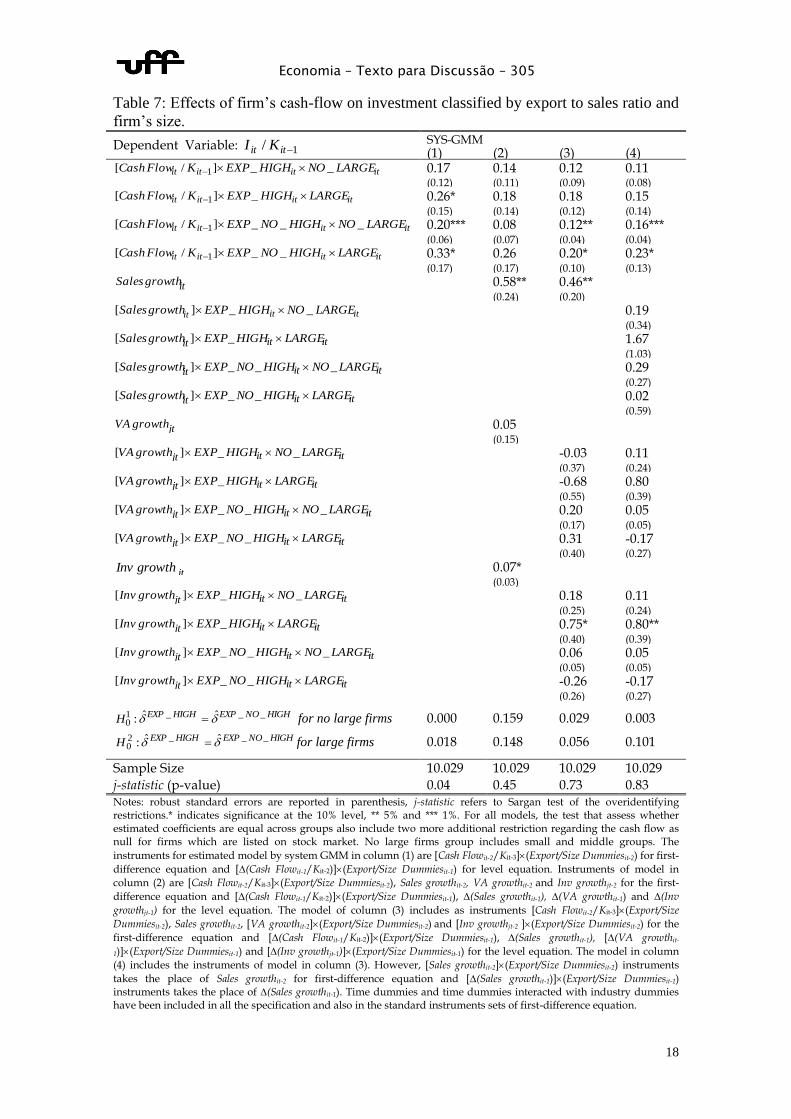
Table 7 reports the outcomes related to the models where variables are classified by
firm’s size and by the firm’s degree of exports to sales ratio, together. One should note
that, as shown in Table 5, both, no-exporters as well as low-export firms are credit
constrained and coefficients associated to them are statistically equal across the two
groups. In this sense, we reclassify them into the following groups: itHIGHNOEXP __
referring to firms with exports to sales ratio which falls below the 50th
percentile of the
export to sales ratio distribution, and itHIGHEXP _ indicates the opposite.
Considering the same export group, with the exception of model 2, firm’s size does
not influence the impact of cash flow on investment, especially when dummies
interactions are extended to the control variables. Similarly to the general results of
Table 5, the cash flow coefficient is statistically null for large exporters. Focusing on
firms with significant cash flow impact, i.e., the no-high exporters group (firms with
zero or low export to ratio sales), there is not strong evidence that the coefficients across
these two groups are different.
In this sense, interacting export groups to the firm’s size do not affect the mainly
results reported in Table 5. It suggests that export status proposed here does not capture
size effect. Otherwise, as discussed, this classification may be associated to our
perspective, i.e. the degree of firm’s external financial constraint.
Finally, one caveat with the above analysis is that there are too few firms that are
simultaneously listed on stock market and small, so comparison between public versus
closed small firms lacks robustness. Otherwise, results here are in line with those
obtained when we interact size and export capacity, what give us more confidence that
the influence of both being listed on stock markets and export capacity are beyond any
possible correlation with size: while in general no-large firms are credit-constrained,
this restriction was softened for firms in this group who are listed on the stock market,
or those who attained significant revenues from exports.
Economia – Texto para Discussão – 305
18
Table 7: Effects of firm’s cash-flow on investment classified by export to sales ratio and
firm’s size.
Dependent Variable: 1/ itit KI SYS-GMM (1) (2) (3) (4)
itititit LARGENOHIGHEXPKFlowCash __]/[ 1 0.17 0.14 0.12 0.11 (0.12) (0.11) (0.09) (0.08)
itititit LARGEHIGHEXPKFlowCash _]/[ 1 0.26* 0.18 0.18 0.15 (0.15) (0.14) (0.12) (0.14)
itititit LARGENOHIGHNOEXPKFlowCash ___]/[ 1 0.20*** 0.08 0.12** 0.16*** (0.06) (0.07) (0.04) (0.04)
itititit LARGEHIGHNOEXPKFlowCash __]/[ 1 0.33* 0.26 0.20* 0.23* (0.17) (0.17) (0.10) (0.13)
itgrowthSales 0.58** 0.46** (0.24) (0.20)
ititit LARGENOHIGHEXPgrowthSales __][ 0.19 (0.34)
ititit LARGEHIGHEXPgrowthSales _][ 1.67 (1.03)
ititit LARGENOHIGHNOEXPgrowthSales ___][ 0.29 (0.27)
ititit LARGEHIGHNOEXPgrowthSales __][ 0.02 (0.59)
jtgrowthVA 0.05 (0.15)
ititjt LARGENOHIGHEXPgrowthVA __][ -0.03 0.11 (0.37) (0.24)
ititjt LARGEHIGHEXPgrowthVA _][ -0.68 0.80 (0.55) (0.39)
ititjt LARGENOHIGHNOEXPgrowthVA ___][ 0.20 0.05 (0.17) (0.05)
ititjt LARGEHIGHNOEXPgrowthVA __][ 0.31 -0.17 (0.40) (0.27)
jtgrowthInv 0.07* (0.03)
ititjt LARGENOHIGHEXPgrowthInv __][ 0.18 0.11 (0.25) (0.24)
ititjt LARGEHIGHEXPgrowthInv _][ 0.75* 0.80** (0.40) (0.39)
ititjt LARGENOHIGHNOEXPgrowthInv ___][ 0.06 0.05 (0.05) (0.05)
ititjt LARGEHIGHNOEXPgrowthInv __][ -0.26 -0.17 (0.26) (0.27)
HIGHNOEXPHIGHEXPH ___10
ˆˆ: for no large firms 0.000 0.159 0.029 0.003
HIGHNOEXPHIGHEXPH ___20
ˆˆ: for large firms 0.018 0.148 0.056 0.101
Sample Size 10.029 10.029 10.029 10.029
j-statistic (p-value) 0.04 0.45 0.73 0.83 Notes: robust standard errors are reported in parenthesis, j-statistic refers to Sargan test of the overidentifying restrictions.* indicates significance at the 10% level, ** 5% and *** 1%. For all models, the test that assess whether estimated coefficients are equal across groups also include two more additional restriction regarding the cash flow as null for firms which are listed on stock market. No large firms group includes small and middle groups. The
instruments for estimated model by system GMM in column (1) are [Cash Flowit-2/Kit-3](Export/Size Dummiesit-2) for first-
difference equation and [∆(Cash Flowit-1/Kit-2)](Export/Size Dummiesit-1) for level equation. Instruments of model in
column (2) are [Cash Flowit-2/Kit-3](Export/Size Dummiesit-2), Sales growthit-2, VA growthit-2 and Inv growthjt-2 for the first-
difference equation and [∆(Cash Flowit-1/Kit-2)](Export/Size Dummiesit-1), ∆(Sales growthit-1), ∆(VA growthit-1) and ∆(Inv
growthjt-1) for the level equation. The model of column (3) includes as instruments [Cash Flowit-2/Kit-3](Export/Size
Dummiesit-2), Sales growthit-2, [VA growthit-2](Export/Size Dummiesit-2) and [Inv growthjt-2 ](Export/Size Dummiesit-2) for the
first-difference equation and [∆(Cash Flowit-1/Kit-2)](Export/Size Dummiesit-1), ∆(Sales growthit-1), [∆(VA growthit-
1)](Export/Size Dummiesit-1) and [∆(Inv growthjt-1)](Export/Size Dummiesit-1) for the level equation. The model in column
(4) includes the instruments of model in column (3). However, [Sales growthit-2](Export/Size Dummiesit-2) instruments
takes the place of Sales growthit-2 for first-difference equation and [∆(Sales growthit-1)](Export/Size Dummiesit-1) instruments takes the place of ∆(Sales growthit-1). Time dummies and time dummies interacted with industry dummies have been included in all the specification and also in the standard instruments sets of first-difference equation.

Economia – Texto para Discussão – 305
19
7. CONCLUSION
In this paper, we evaluate whether Brazilian firms are credit constrained and, especially,
which conditions prevail for the existence of credit restrictions. Our results back up
previous studies using Brazilian data, which say that they are credit restricted.
Moreover, we found that Brazilian firms’ cash flow to investment elasticity is on
average 5 times larger than British firms’ elasticity, suggesting a greater degree of
constraints in Brazilian credit market.9 Despite confirming what has been previously
investigated, we found that firms not listed on the stock market are credit constraint yet
those listed are not. Terra (2003) and Aldrighi and Bisinha (2010) found that firms
listed on the stock market are credit constrained.
Regarding results on firms’ size, our findings go on the usual direction of international
literature, where credit constraints are softened for larger firms, while in Aldrighi and
Bisinha (2010) prevail the opposite result and Terra (2003) can only replicate a result
similar to ours in a limited period of years in her sample. In addition, we find that
companies more devoted to exports, measured as the ratio exports/sales, are not credit
constrained, whereas firms that export below the median are credit restricted. Our
results are valid, indeed, when one considers the size’s bias. That is to say, even small
companies that are public or high exporters do not experience credit restrictions,
accordingly to our outcomes.
Yet, it is important to note that not only does the period of time are quite different but
also the composition of firms covered by those studies, and we should also note that the
latter authors ignore some important methodological issues which are acknowledged in
this paper, such as endogeneity and sector opportunities investments controls.
Our findings in this paper may also have some valuable policy implications. First, we
have noticed that credit restriction occurs with firms generating resources around their
capital stock level, in other words, when ratio of cash flow over capital is close to one.
Having those results in mind, this might be an indication on which firm is restricted to
invest, since they are already investing all they can with their own resources. Thus, if
this ratio is close to one, those firms might be target for public policy. However, other
criteria are also relevant for public policy design. For instance, investment in intangible
assets was not considered in this investigation, and therefore some apparently non-credit
restricted firms might depend on internal funds to invest in innovation. Thus, we can´t
use our measure of credit restriction as the only criteria for public policy design, and
some other targets for public funding must be elected, as exemplified by the current
focus of BNDES in innovation.
Second, in a developing country like Brazil, where capital is scarce and long term
credit is usually provided by state-owned banks, availability of other sources of funds
are vital for accelerating economic growth. If we understand the stock market as an
“inside” source of funds for firms in a country and export capacity as a proxy for
“outside” source of funds, once export revenue may be seen as a collateral to get access
to international financing, our results suggest that both were valuable for mitigating
credit restrictions in Brazilian firms.
Of course, what our methodology strictly permits to investigate is a comparison of the
levels of credit constraints among firms with certain characteristics (size, listed or not
on the Brazilian stock markets and export capacity), and some hidden factors may
determine both the degree of credit constraints and these characteristics. But, at the
9 This result is achieved by comparing our coefficient estimator on Table 3 to Carpenter and Guariglia’s
(2008).

Economia – Texto para Discussão – 305
20
same time, our results show that the categories mentioned systematic reduce credit
constraints for Brazilian firms, even after controlling for a series of observable variables
that may impact the investment decision, reinforcing our suspicion that there is indeed a
casual effect. Whether this is the case, we can propose that government efforts should
be made, for instance, to develop the stock market (or to help firms to achieve the
standards required to go public) and to stimulate exports, in this way contributing to
alleviate credit constraints of domestics firms and sponsoring their investments. It is
indeed what BNDES does by its subsidiaries: BNDESPAR; and BNDES-Exim. In the
former, BNDES offers support for firms aiming to offer their shares in the stock market,
while export support is offered by the latter. At the same time, support from BNDES
must not be restricted to these kind of programs, and indeed large and well established
exporting and already listed firms should receive financing, for instance for projects
generating positive externalities in the economy.
In sum, it is feasible to emphasize that there is room for public policy implications
considering our credit restriction results. BNDES is aware of this market failure and its
operational policy proposes different types of support to overcome this shortcoming.
Moreover, actual world economic situation, after the economic crisis initiated in 2008,
presents even more challenging scenarios for governments to address this market
failure. Certainty is the importance of governments to mitigate credit restriction for
private firms.
REFERENCES
Allayannis, G., and Mozumdar, A. (2004) “The impact of negative cash flow and
influential observations on investment-cash flow sensitivity estimates” Journal of
Banking and Finance Vol. 28, No. 5, 901-930.
Aldrighi, D. and Bisinha, R. (2010) “Restrição financeira em empresas com ações
negociadas na Bovespa” Revista Brasileira de Economia, Vol. 64, No. 1, 25-47
Arellano, M., and Bover, O. (1995) “Another look at the instrumental variable
estimation of error-components models” Journal of Econometrics, Vol. 68, No. 1, 29-
51.
Banerjee, A. and Duflo, E. (2005) “Growth Theory through the Lens of Development",
in Economics Handbook of Economic Growth, Vol. 1, Part A, 473-552.
Baun, C. F,; Schäfer, D.; Talavera, O. (2011) “The impact of the financial system’s
structure on firms’ financial constraints” Journal of International Money and Finance,
No. 30, p. 678-691.
Blundell, R., and Bond, S. (1998) “Initial conditions and moment restrictions in
dynamic panel-data models” Journal of Econometrics, Vol. 87, No. 1, 115-143.
Bond, S. and Meghir, C. (1994) “Dynamic investment models and the firm`s financial
policy” Review of Economic Studies, Vol. 61, No. 2, 197-222.
Carpenter, R. and Guariglia, A. (2008) “Cash flow, investment, and investment
opportunities: new tests using UK panel data” Journal of Banking and Finance, Vol. 32,
No. 9, 1894-1906.

Economia – Texto para Discussão – 305
21
Cleary, S. (1999) “The relationship between firm investment and financial status” The
Journal of Finance, Vol. 54, No. 2, 673–692.
Cleary, S., Povel, P. and Raith M. (2007) “The U-shaped investment curve: Theory and
evidence” Journal of Financial and Quantitative Analysis, Vol. 42, No. 1, 1–39.
Fazzari, S., Hubbard, R. and Petersen, B. (1988) “Financing constraints and corporate
investments” Brookings Papers on Economic Activity 1: 141–206.
Guariglia, A. (2008). “Internal financial constraints, external financial constraints, and
investment choice: evidence from a panel of UK firms. Journal of Banking and Finance
32, 1795-1809.
Guariglia, A., Liu, X. and Song, L. (2011) “Internal finance and growth:
microeconometric evidence on Chinese firms. Journal of Development Economics, Vol.
96, No. 1, 79-94.
Hubbard, G. (1998) “Capital-market imperfections and investments” Journal of
Economic Literature, Vol. 36, 193-225.
Kaplan, S. and Zingales, L. (1997) “Do investment cash flow sensitivities provide
useful measures of financing constraints?” Quarterly Journal of Economics, Vol. 112,
No. 1, 169–215.
Stiglitz, J. and Weiss, A. (1981) “Credit Rationing in Markets with Imperfect
Information” American Economic Review, Vol. 71, No. 3, 393-410.
Terra, M. C.. 2003 “Credit constraints in brazilian firms: evidence from panel data”
Revista Brasileira de Economia, Vol. 57, No. 2, 443-464.