Text Searching: Theory and Practice

Ricardo A. Baeza-Yates and Gonzalo Navarro

Depto. de Ciencias de la Computacion, Universidad de Chile, Casilla 2777, Santiago, Chile.E-mail: rbaeza,gnavarro@dcc.uchile.cl.

Abstract

We present the state of the art of the main component of text retrieval systems: the searchengine. We outline the main lines of research and issues involved. We survey the relevanttechniques in use today for text searching and explore the gap between theoretical and practicalalgorithms. The main observation is that simpler ideas are better in practice.

In theory, The best theory is inspired by practice.there is no difference between theory and practice. The best practice is inspired by theory.In practice, there is. Donald E. Knuth

Jan L.A. van de Snepscheut

1 Introduction

Full text retrieval systems have become a popular way of providing support for text databases.The full text model permits locating the occurrences of any word, sentence, or simply substringin any document of the collection. Its main advantages, as compared to alternative text retrievalmodels, are simplicity and efficiency. From the end-user point of view, full text searching of on-line documents is appealing because valid query patterns are just any word or sentence of thedocuments. In the past, alternatives to the full-text model, such as semantic indexing, hadreceived some attention. Nowadays, those alternatives are confined to very specific domainswhile most text retrieval systems used in practice rely, in one way or another, on the full textmodel.

The main component of a full text retrieval system is the text search engine. The task of thisengine is to retrieve the occurrences of query patterns in the text collection. Patterns can rangefrom simple words, phrases or strings to more sophisticated forms such as regular expressions.The efficiency of the text search engine is usually crucial for the overall success of the databasesystem.

It is possible to build and maintain an index over the text, which is a data structure designedto speed up searches. However, (i) indices take space, which may or may not be available;(ii) indices take time to build, so construction time must be amortized over many searches,which outrules indexing for texts that will disappear soon such as on-line news; (iii) indicesare relatively costly to maintain upon text updates, so they may not be useful for frequentlychanging text such as in text editors; and (iv) the search without an index may be fast enoughfor texts of several megabytes, depending on the application. For these reasons, we may find textsearch systems that rely on sequential search (without index), indexed search, or a combinationof both.

1

In this chapter we review the main algorithmic techniques to implement a text search engine,with or without indices. We will focus on the most recent and relevant techniques in practice,although we will cover the main theoretical contributions to the problem and highlight thetension between theoretically and practically appealing ideas. We will show how simpler ideaswork better in practice. As we do not attempt to fully cover all the existing developments, werefer the interested reader to several books that cover the area in depth [31, 22, 58, 13, 71, 25, 34].

2 Basic Concepts

We start by defining some concepts. Let text be the data to be searched. This data may bestored in one or more files, a fact that we disregard for simplicity. Text is not necessarily naturallanguage, but just a sequence (or string) of characters. In addition, some pieces of the text mightnot be retrievable (for example, if a text contains images or non-searchable data), or we maywant to search different pieces of text in different ways. For example, in GenBank registersone finds DNA streams mixed with English descriptions and metadata, and retrieval over thoseparts of the database are very different processes.

2.1 The Full Text Model

The text database can be viewed as a very long string of data. Often text has little or nostructure, and in many applications we wish to process the text without concern for the structure.This is typically the case of biological or multimedia sequences. As oriental languages such asChinese, Japanese, and Korean Kanji are difficult to segment into words, texts written in thoselanguages are usually regarded as a very long string too. For this view of the text, we usuallywant to retrieve any text substring.

Natural language texts written in Western languages can be regarded as a sequence of words.Each word is a maximal string not including any symbol from a special separator set (such as ablank space). Examples of such collections are dictionaries, legal cases, articles on wire services,scientific papers, etc. In this case we might want to retrieve only words or phrases, or also anytext substring.

Optionally, a text may have a structure. The text can be logically divided into documents,and each document into fields. Alternatively, the text may have a complex hierarchical or graphstructure. This is the case of text databases structured using XML, SGML or HTML, wherewe might also query the structure of the text. In this chapter we will ignore text structure andregard it as a sequence of characters or words.

2.2 Notation

We introduce some notation now. A string S of length |S| = s will be written as S1...s. Itsi-th character will be Si and a string formed by characters i to j of S will be written Si...j.Characters are drawn from an alphabet Σ of size σ > 1. String S is a prefix of SS′, a suffix ofS′S, and a substring of S′SS′′, where S′ and S′′ are arbitrary strings.

The most basic problem in text searching is to find all the positions where a pattern P =P1...m occurs in a text T = T1...n, m ≤ n. In some cases one is satisfied with any occurrence ofP in T , but in this chapter we will focus on the most common case where one wants them all.Formally, the search problem can be written as retrieving |X|, T = XPY . More generally,pattern P will denote a language, L(P ) ⊆ Σ∗, and our aim will be to find the text occurrencesof any string in that language, formally |X|, T = XP ′Y, P ′ ∈ L(P ).

2

We will be interested both in worst-case and average-case time and space complexities. Weremind that the worst case is the maximum time/space the algorithm may need over everypossible text and pattern, while the average case is the mean time over all possible texts andpatterns. For average case results we assume that pattern and text characters are uniformlyand independently distributed over the σ characters of the alphabet. This is usually not true,but it is a reasonable model in practice.

We make heavy use of bit manipulations inside computer words, so we need some furthernotation for these. Computer words have w bits (typically w = 32, 64 or 128), and sequenceof bits in a computer word are written right to left. The operations to manipulate them areinherited from C language: “|” is the bitwise “or”, “&” is the bitwise “and”, “<<” shifts all thebits to the left (that is, the bit at position i moves to position i + 1) and enters a zero at therightmost position, “>>” shifts to the right and enters a zero at the leftmost position (unsignedsemantics), “∧” is the bitwise exclusive or (xor), and “∼” complements all the bits. We can alsoperform arithmetic operations on the computer words such as “+” and “−”.

2.3 Text Suffixes

Observe that any occurrence of P in T is a prefix of a suffix of T (this suffix is PY or P ′Y inour formal definition). The concept of prefix and suffix plays a central role in text searching. Inparticular, a model that has proven extremely useful, and that marries very well with the fulltext model, is to consider the text as the set of its suffixes.

We assume that the text to be searched is a single string padded at its right end with aspecial terminator character, denoted “$” and smaller than any other. A text suffix is simply asuffix of T , that is, the sequence of characters starting at any position of the text and continuingto the right. Given the terminator, all the text suffixes are different, and no one is a prefix ofany other. Moreover, there is a one-to-one correspondence between text positions i and textsuffixes Ti...n.

Under this view, the search problem is to find all the text suffixes starting with P (orP ′ ∈ L(P )).

2.4 Tries

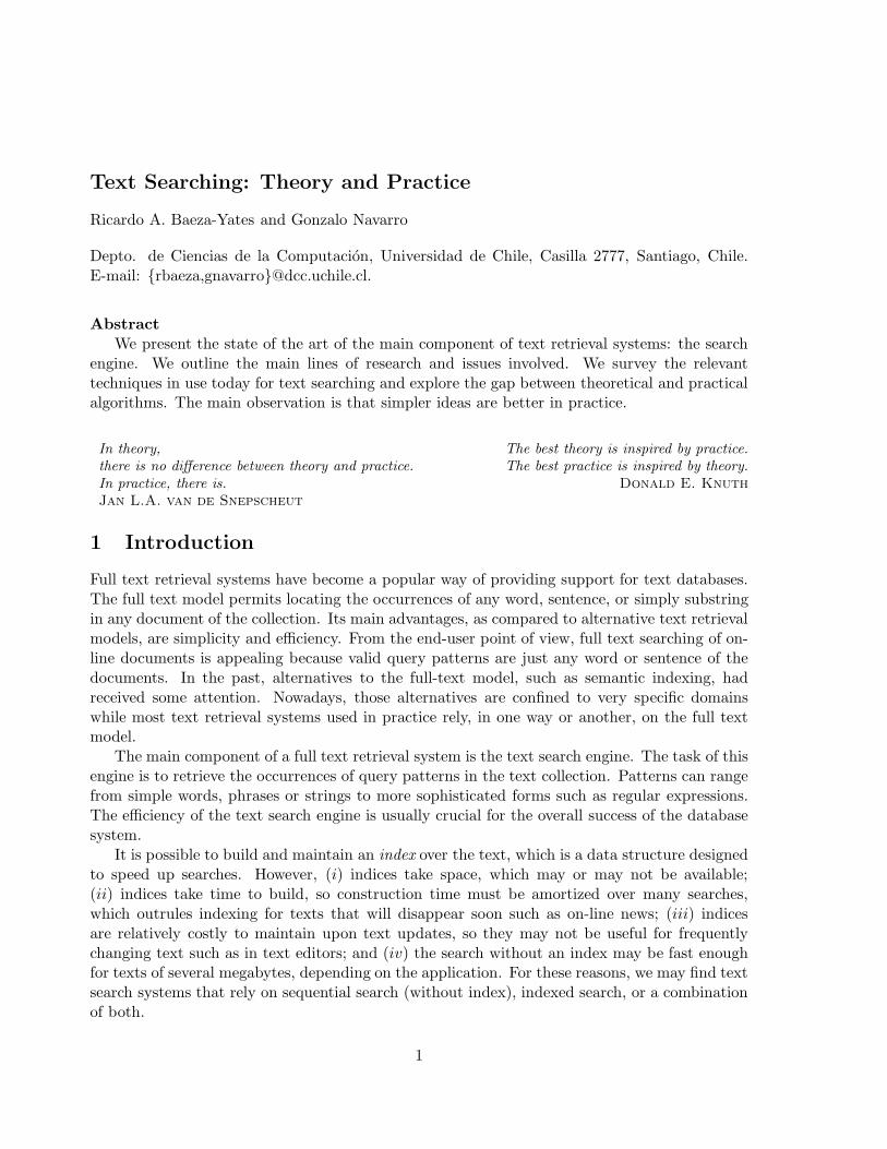
Finally, let us introduce an extremely useful data structure for text searching. It is called atrie, and is a data structure that stores a set of strings and permits determining in time O(|S|)whether string S is in the set, no matter how many strings are stored in the trie. A trie on a setof strings is a tree with one leaf per string and one internal node per different proper prefix of astring. There is an edge labeled c from every node representing prefix S to the node representingprefix Sc. The root represents the empty string. Figure 1 (left) illustrates.

In order to search for S in the trie, we start at the root and follow edge S1, if it exists. Ifwe succeed, we follow edge S2 from the node we arrived at, and so on until either (i) we cannotfind the proper edge to follow, in which case S is not in the set, or (ii) we use all the charactersin S, and if the node arrived at stores a string, we have found S. Note that it is also easy todetermine whether S is a prefix of some string stored in the trie: We search for S and all thesubtree of the node arrived at contains the strings whose prefix is S.

We might add a special string terminator “$” to all the strings so as to ensure that no stringis a prefix of another in the set. In this case there is a one-to-one correspondence between trieleaves and stored strings. To save some space, we usually put the leaves as soon as the stringprefix is unique. When the search arrives at such a leaf, the search process continues comparingthe search string against the string stored at the leaf. Figure 1 (right) illustrates.

3

a b

d m a

a a e r

l n l b

i d i a

a a e r

aadalia amanda amelie

barbara

ada

a b

d m

a

barbara

adaliaada

l$

a eamelieamanda

Figure 1: A trie over the strings "ada", "amanda", "amelie", "barbara" and "adalia". Onthe left, basic formulation. On the right, the version used in practice.

3 Sequential Text Search

In this section we assume that no index on the text is available, so we have to scan all the textin order to report the occurrences of P . We start with simple string patterns and later considermore sophisticated searches.

To better understand the problem, let us consider which would be its naive solution. Considerevery possible initial position of an occurrence of P in T , that is, 1 . . . n−m + 1. For each suchinitial position i, compare P with Ti...i+m−1. Report an occurrence whenever the two stringsmatch. The worst case complexity of this algorithm is O(mn). Its average case complexity,however, is O(n), since on average we have to compare σ/(σ − 1) characters before two stringsmismatch. Our aim is to do better.

From a theoretical viewpoint, this problem is basically solved, except for very focused ques-tions that still remain.

• The worst-case complexity is clearly Ω(n) character inspections (for the exact constant see[18]). This has been achieved by Knuth-Morris-Pratt (KMP) algorithm [41] using O(m)space.

• The average-case complexity is Ω(n logσ(m)/m) [76]. This has been achieved by BackwardDAWG Matching (BDM) algorithm [21] using O(m) space. The algorithm can be madeworst-case optimal at the same time (e.g., TurboBDM and TurboRF variants [21]).

• Optimal worst-case algorithms with O(1) extra space exist (the first was [28]), while thesame problem is open for the average case.

If one turns attention to practical matters, however, the above algorithms are in severalaspects unsatisfactory. For example, in practice KMP is twice as slow as the naive searchalgorithm, which can be programmed with three lines of code or so. BDM, on the other hand,is rather complicated to implement and not so fast for many typical text searching scenarios.For example, BDM is a good choice to search for patterns of length m = 100 on DNA text,but when it comes to search for words and phrases (of length typically less than 30) in natural

4

language text, it is outperformed by far by a simple variant of Boyer-Moore due to Horspool[36], which also can be coded in a few lines.

In this section we will consider two successful approaches to text searching. These are re-sponsible for most of the relevant techniques in use today. In both approaches we will explorethe relation between theoretically and practically appealing algorithms, and we will show thatusually the best practical algorithms are simplified versions of their complex theoretical coun-terparts. The first approach is the use of automata, which theoretical algorithms convert todeterministic form while practical algorithms simulate in their simple and regular nondetermin-istic form. The second approach is the use of filtering, where theoretical algorithms minimizethe number of character inspections at a considerable extra processing cost, while practicalalgorithms use simpler criteria that inspect more characters but are faster in practice.

3.1 Automata

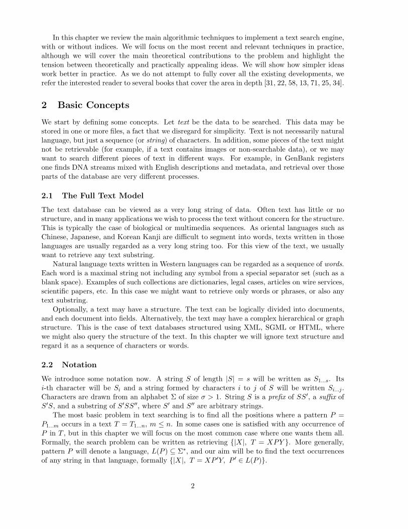
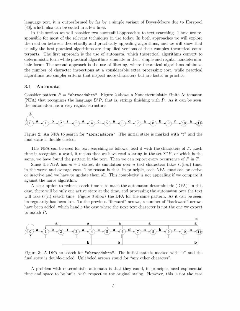
Consider pattern P = "abracadabra". Figure 2 shows a Nondeterministic Finite Automaton(NFA) that recognizes the language Σ∗P , that is, strings finishing with P . As it can be seen,the automaton has a very regular structure.

a r a c d b r a

Σ

b a a0 1 2 3 4 5 6 7 8 9 1110

Figure 2: An NFA to search for "abracadabra". The initial state is marked with “〉” and thefinal state is double-circled.

This NFA can be used for text searching as follows: feed it with the characters of T . Eachtime it recognizes a word, it means that we have read a string in the set Σ∗P , or which is thesame, we have found the pattern in the text. Then we can report every occurrence of P in T .

Since the NFA has m + 1 states, its simulation over n text characters takes O(mn) time,in the worst and average case. The reason is that, in principle, each NFA state can be activeor inactive and we have to update them all. This complexity is not appealing if we compare itagainst the naive algorithm.

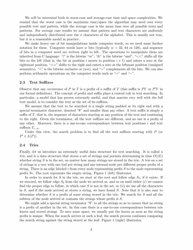
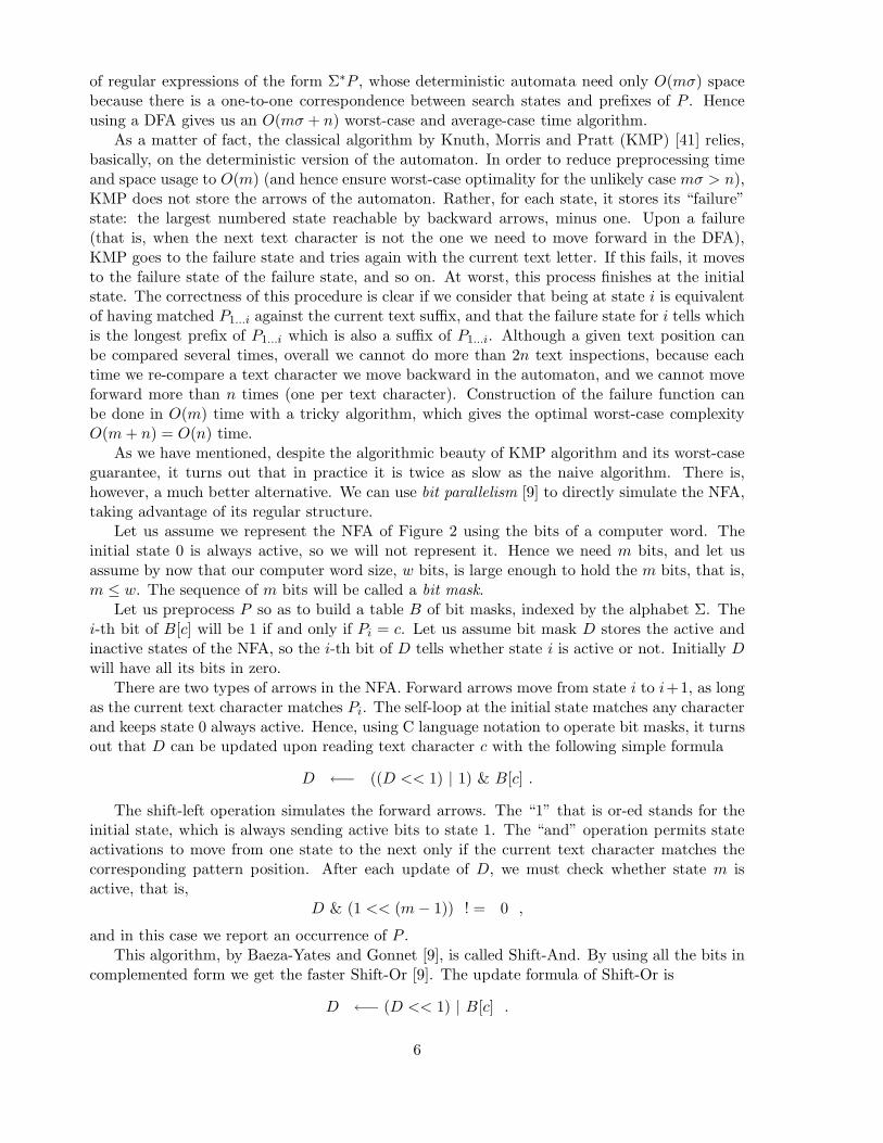
A clear option to reduce search time is to make the automaton deterministic (DFA). In thiscase, there will be only one active state at the time, and processing the automaton over the textwill take O(n) search time. Figure 3 shows the DFA for the same pattern. As it can be seen,its regularity has been lost. To the previous “forward” arrows, a number of “backward” arrowshave been added, which handle the case where the next text character is not the one we expectto match P .

a r a c d b r ab a a0 1 2 3 4 5 6 7 8 9 1110

aa

b

a

b

aca

b

Figure 3: A DFA to search for "abracadabra". The initial state is marked with “〉” and thefinal state is double-circled. Unlabeled arrows stand for “any other character”.

A problem with deterministic automata is that they could, in principle, need exponentialtime and space to be built, with respect to the original string. However, this is not the case

5

of regular expressions of the form Σ∗P , whose deterministic automata need only O(mσ) spacebecause there is a one-to-one correspondence between search states and prefixes of P . Henceusing a DFA gives us an O(mσ + n) worst-case and average-case time algorithm.

As a matter of fact, the classical algorithm by Knuth, Morris and Pratt (KMP) [41] relies,basically, on the deterministic version of the automaton. In order to reduce preprocessing timeand space usage to O(m) (and hence ensure worst-case optimality for the unlikely case mσ > n),KMP does not store the arrows of the automaton. Rather, for each state, it stores its “failure”state: the largest numbered state reachable by backward arrows, minus one. Upon a failure(that is, when the next text character is not the one we need to move forward in the DFA),KMP goes to the failure state and tries again with the current text letter. If this fails, it movesto the failure state of the failure state, and so on. At worst, this process finishes at the initialstate. The correctness of this procedure is clear if we consider that being at state i is equivalentof having matched P1...i against the current text suffix, and that the failure state for i tells whichis the longest prefix of P1...i which is also a suffix of P1...i. Although a given text position canbe compared several times, overall we cannot do more than 2n text inspections, because eachtime we re-compare a text character we move backward in the automaton, and we cannot moveforward more than n times (one per text character). Construction of the failure function canbe done in O(m) time with a tricky algorithm, which gives the optimal worst-case complexityO(m + n) = O(n) time.

As we have mentioned, despite the algorithmic beauty of KMP algorithm and its worst-caseguarantee, it turns out that in practice it is twice as slow as the naive algorithm. There is,however, a much better alternative. We can use bit parallelism [9] to directly simulate the NFA,taking advantage of its regular structure.

Let us assume we represent the NFA of Figure 2 using the bits of a computer word. Theinitial state 0 is always active, so we will not represent it. Hence we need m bits, and let usassume by now that our computer word size, w bits, is large enough to hold the m bits, that is,m ≤ w. The sequence of m bits will be called a bit mask.

Let us preprocess P so as to build a table B of bit masks, indexed by the alphabet Σ. Thei-th bit of B[c] will be 1 if and only if Pi = c. Let us assume bit mask D stores the active andinactive states of the NFA, so the i-th bit of D tells whether state i is active or not. Initially Dwill have all its bits in zero.

There are two types of arrows in the NFA. Forward arrows move from state i to i+1, as longas the current text character matches Pi. The self-loop at the initial state matches any characterand keeps state 0 always active. Hence, using C language notation to operate bit masks, it turnsout that D can be updated upon reading text character c with the following simple formula

D ←− ((D << 1) | 1) & B[c] .

The shift-left operation simulates the forward arrows. The “1” that is or-ed stands for theinitial state, which is always sending active bits to state 1. The “and” operation permits stateactivations to move from one state to the next only if the current text character matches thecorresponding pattern position. After each update of D, we must check whether state m isactive, that is,

D & (1 << (m− 1)) ! = 0 ,

and in this case we report an occurrence of P .This algorithm, by Baeza-Yates and Gonnet [9], is called Shift-And. By using all the bits in

complemented form we get the faster Shift-Or [9]. The update formula of Shift-Or is

D ←− (D << 1) | B[c] .

6

ShiftOr(T1...n, P1...m)

for c ∈ Σ do B[c]← (1 << m)− 1for j ∈ 1 . . . m do B[pj] ← B[pj] & ∼ (1 << (j − 1))D ← (1 << m)− 1for i ∈ 1 . . . n do

D ← (D << 1) | B[ti]if D & (1 << (m− 1)) = 0

then P occurs at Ti−m+1...i

Figure 4: Shift-Or algorithm.

Preprocessing of P needs O(m + σ) time and O(σ) space. The text scanning phase is O(n).Hence we get a very simple algorithm that is O(σ + m + n) time and O(σ) space in the worstand average case. More important, Shift-Or is faster than the naive algorithm and can be codedin a few lines. Figure 4 gives its pseudocode.

For patterns exceeding the computer word size (m > w), a multi-word implementation canbe considered. Hence we will have to update ⌈m/w⌉ computer words per text character andthe worst case search time will be O(m + (σ + n)⌈m/w⌉). In practice, since the probabilityof activating a state larger than w is minimal (1/σw), it is advisable to just search for P1...w

using the basic algorithm and compare Pw+1...m directly against the text when P1...w matches.Verifications add n/σw ×O(1) extra time, so the average time remains O(σ + m + n).

3.2 Filtering

The previous algorithms try to do their best under the assumption that one has to inspect everytext character. In the worst case one cannot do better. However, on average, one can discardlarge text areas without actually inspecting all their characters. This concept is called filteringand was invented by Boyer and Moore [15], only a few years later than KMP (but they werepublished the same year).

A key concept in filtering is that of a text window, which is any range of text positions of theform i . . . i + m − 1. The search problem is that of determining which text windows match P .Filtering algorithms slide the window left to right on the text. At each position, they inspectsome text characters in the window and collect enough information so as to determine whetherthere is a match or not in the current window. Then, they shift the window to a new position.Note that the naive algorithm can be seen as a filtering algorithm that compares P and the textwindow left to right, and always shifts by one position.

The original idea of Boyer-Moore (BM) algorithms is to compare P and the text windowright to left. Upon a match or mismatch, they make use of the information collected in thecomparison of the current window so as to shift it by at least one character. The originalBoyer-Moore algorithms used the following rules to shift the window as much as possible:

• If we have read suffix s from the window and this has matched the same suffix of P , thenwe can shift the window until s (in the text) aligns with the last occurrence of s in P1...m−1.If there is no such occurrence, then we must align the longest suffix of s that is also a prefixof P .

7

• If we have read characters from the window and the mismatch has occurred at a characterc, then we can shift the window until that position is aligned to a c in P .

In fact, the original BM algorithm precomputes the necessary data to implement only thelast heuristic (the first was introduce in the KMP paper), and at each moment it uses the onegiving the largest shift. Although in the worst case the algorithm is still O(mn), on average itis O(n/min(m,σ)). This was the first algorithm that did not compare all the text characters.The algorithm was later extended to make it O(n) in the worst case [17].

In practice, the algorithm was rather complicated to implement, not to mention if one hasto ensure linear worst-case complexity. A practical improvement was obtained by noting that,for large enough alphabets, the second heuristic usually gave good enough shifts (the originalidea). Hence computing two shifts to pick the largest was not worth the cost. The resultingalgorithm, called Simplified BM, is simpler than BM and competitive.

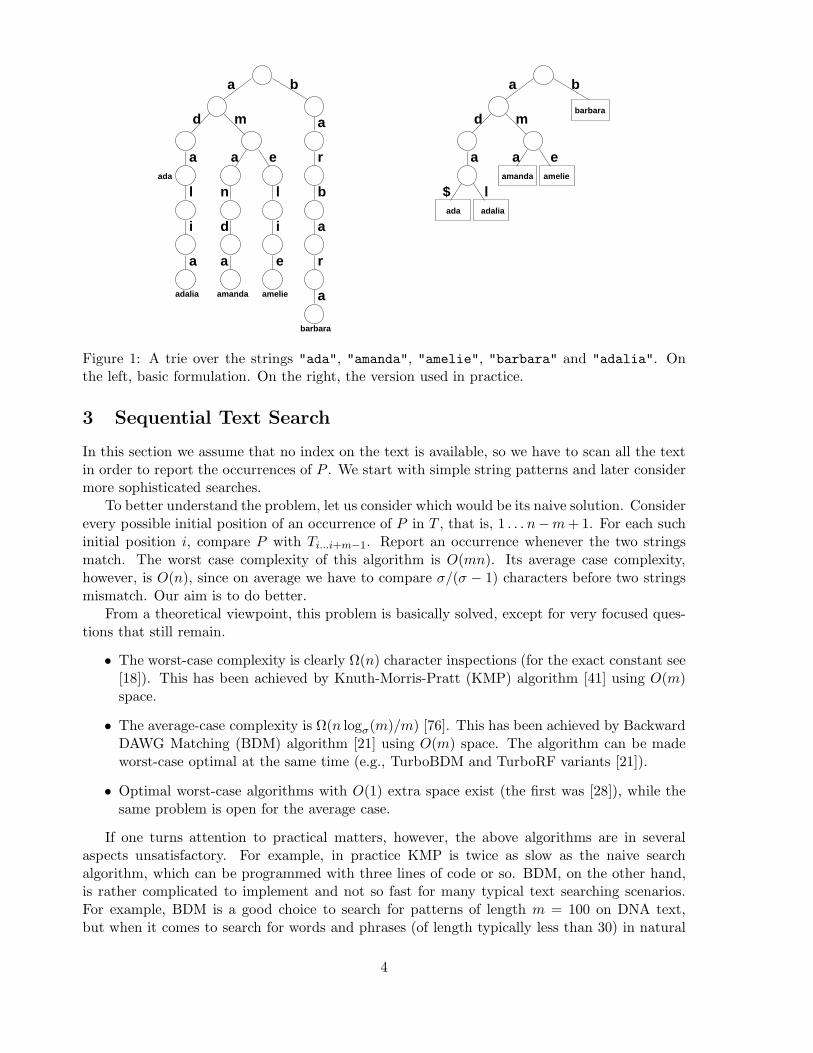
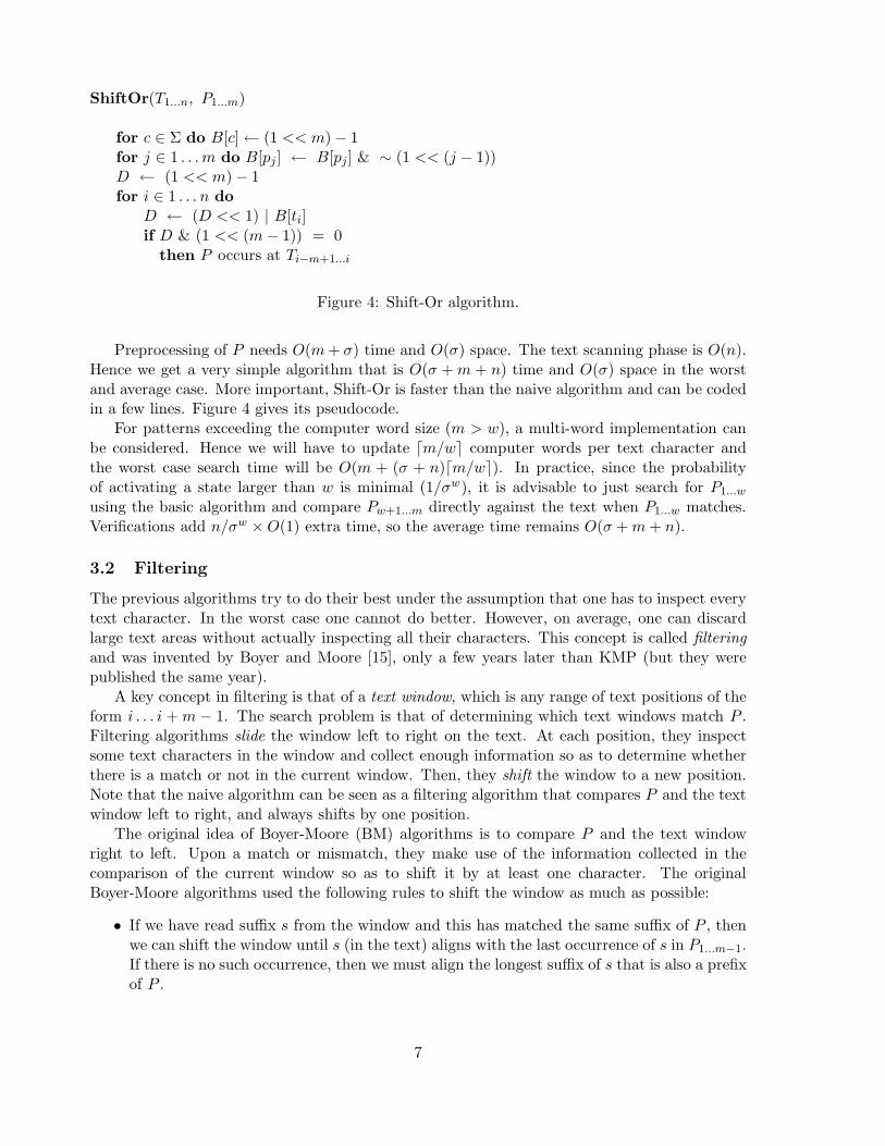
However, even simpler and faster is Horspool algorithm [36]. Pattern and text window arecompared in any order, even left to right (this can be done using a special-purpose machineinstruction that compares chunks of memory). If they are equal, the occurrence is reported.In any case, the last window character is used to determine the shift. For this sake, a table dis built so that d[c] is the distance from the last occurrence of c in P1...m−1 to m. Hence, thewindow starting at text position i can be shifted by d[Ti+m−1]. Figure 5 illustrates.

abracadabra

abracadabra

eda Ttext window

P

last ’a’ in ’abracadabr’

mismatch here d[’a’] = 3d[’b’] = 2d[’c’] = 6d[’d’] = 4d[’r’] = 1d[*] = 11

shift

Figure 5: Example of Horspool algorithm over a window terminating in "eda". In the examplewe assume that P and the window are compared right to left.

Preprocessing requires O(m + σ) time and O(σ) space, while the average search time isstill O(n/min(m,σ)). The algorithm fits in less than ten lines of code in most programminglanguages. A close variant of this algorithm is due to Sunday [62], which uses the text positionfollowing the window instead of the last window position. This makes the search time closer ton/(m + 1) instead of Horspool’s n/m, and is in practice faster than Horspool.

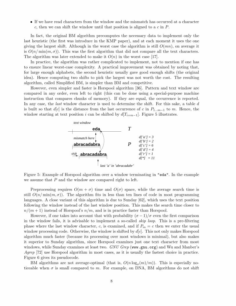
However, if one takes into account that with probability (σ− 1)/σ even the first comparisonin the window fails, it is advisable to implement a so-called skip loop. This is a pre-filteringphase where the last window character, c, is examined, and if Pm = c then we enter the usualwindow processing code. Otherwise, the window is shifted by d[c]. This not only makes Horspoolalgorithm much faster (because its processing over most windows is minimal), but also makesit superior to Sunday algorithm, since Horspool examines just one text character from mostwindows, while Sunday examines at least two. GNU Grep (www.gnu.org) and Wu and Manber’sAgrep [72] use Horspool algorithm in most cases, as it is usually the fastest choice in practice.Figure 6 gives its pseudocode.

BM algorithms are not average-optimal (that is, O(n logσ(m)/m)). This is especially no-ticeable when σ is small compared to m. For example, on DNA, BM algorithms do not shift

8

Horspool(T1...n, P1...m)

for c ∈ Σ do d[c]← mfor j ∈ 1 . . . m− 1 do d[pj ] ← m− ji ← 0while i + m ≤ n do

while i + m ≤ n ∧ ti+m 6= pm do i ← i + d[ti+m]if P1...m−1 = Ti+1...i+m−1

then P occurs at Ti+1...i+m

i ← i + d[ti+m]

Figure 6: Horspool algorithm with skip loop included.

windows by more than 4 positions on average, no matter how large is m.One way to circumvent this weakness is to artificially enlarge the alphabet. This folklore idea

has been reinvented several times, see for example [7, 40, 64]. Say that, instead of consideringjust the last window character to determine the shift, we read the last q characters (that is, thelast window q-gram). We preprocess P so that, for each possible q-gram, we record its smallestdistance to the end of the pattern. Then, we use Horspool as usual. Note that we pay O(q)character inspections to read a q-gram.

The search time of this algorithm is O(σq+m+qn/min(m,σq)), so the optimum is q = logσ mand this yields the average-optimal O(m + n logσ(m)/m). This is the technique used in Agrepfor long patterns. In practice, depending on the architecture, one may take advantage from thefact that the computer word usually can hold a q-gram, and read q-grams in a single machineinstruction, so as to get O(n/m) search time.

3.3 Filtering Using Automata

Another way to see why BM is not average-optimal is that it shifts the window too soon, that is,as soon as it knows that it can be shifted. Since this occurs after O(1) comparisons, the patternis shifted so that it aligns correctly with O(1) window characters, and this occurs for a shift oflength O(σ). Perhaps a bit counterintuitively, one should wait a bit more.

A very elegant algorithm, which was the first in achieving average optimality (and, withsome modifications, worst-case optimality at the same time) is Backward DAWG Matching(BDM) [21], by Crochemore et al. This algorithm combines the use of automata with filteringtechniques.

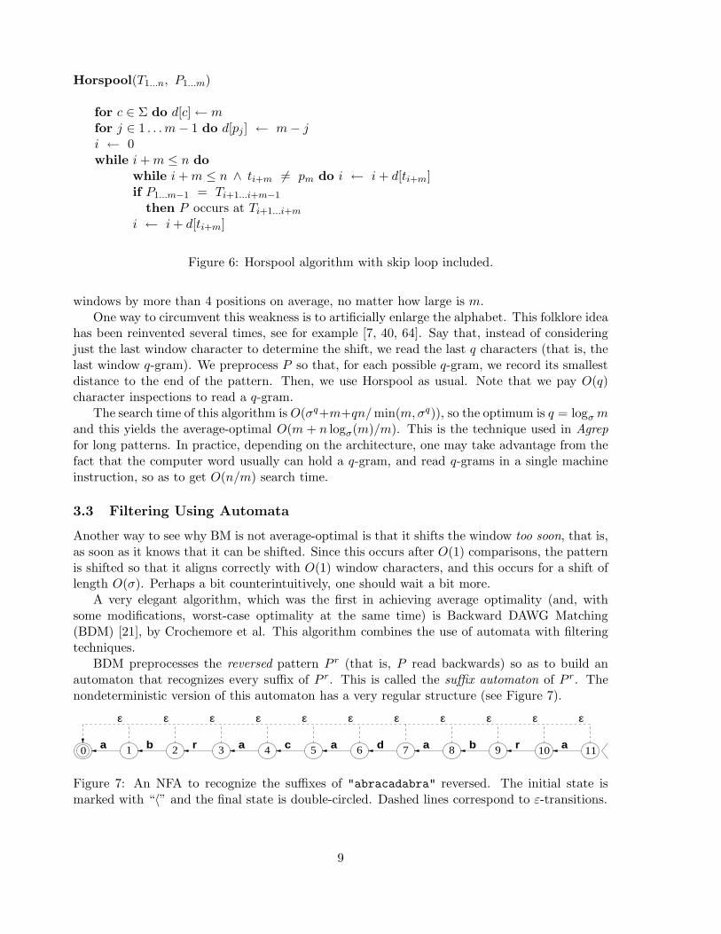
BDM preprocesses the reversed pattern P r (that is, P read backwards) so as to build anautomaton that recognizes every suffix of P r. This is called the suffix automaton of P r. Thenondeterministic version of this automaton has a very regular structure (see Figure 7).

a r a c d b r ab a a1 2 3 4 5 6 7 8 9 11100

εεεεεε εεεεε

Figure 7: An NFA to recognize the suffixes of "abracadabra" reversed. The initial state ismarked with “〈” and the final state is double-circled. Dashed lines correspond to ε-transitions.

9

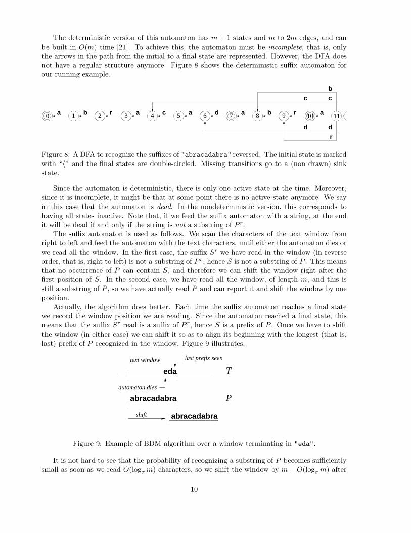
The deterministic version of this automaton has m + 1 states and m to 2m edges, and canbe built in O(m) time [21]. To achieve this, the automaton must be incomplete, that is, onlythe arrows in the path from the initial to a final state are represented. However, the DFA doesnot have a regular structure anymore. Figure 8 shows the deterministic suffix automaton forour running example.

a r a c d b r ab a a1 2 3 4 5 6 7 8 9 11100

c c

b

d d

r

Figure 8: A DFA to recognize the suffixes of "abracadabra" reversed. The initial state is markedwith “〈” and the final states are double-circled. Missing transitions go to a (non drawn) sinkstate.

Since the automaton is deterministic, there is only one active state at the time. Moreover,since it is incomplete, it might be that at some point there is no active state anymore. We sayin this case that the automaton is dead. In the nondeterministic version, this corresponds tohaving all states inactive. Note that, if we feed the suffix automaton with a string, at the endit will be dead if and only if the string is not a substring of P r.

The suffix automaton is used as follows. We scan the characters of the text window fromright to left and feed the automaton with the text characters, until either the automaton dies orwe read all the window. In the first case, the suffix Sr we have read in the window (in reverseorder, that is, right to left) is not a substring of P r, hence S is not a substring of P . This meansthat no occurrence of P can contain S, and therefore we can shift the window right after thefirst position of S. In the second case, we have read all the window, of length m, and this isstill a substring of P , so we have actually read P and can report it and shift the window by oneposition.

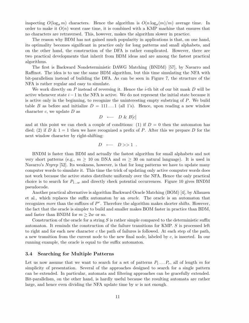
Actually, the algorithm does better. Each time the suffix automaton reaches a final statewe record the window position we are reading. Since the automaton reached a final state, thismeans that the suffix Sr read is a suffix of P r, hence S is a prefix of P . Once we have to shiftthe window (in either case) we can shift it so as to align its beginning with the longest (that is,last) prefix of P recognized in the window. Figure 9 illustrates.

abracadabra

abracadabra

eda Ttext window

P

automaton dies

last prefix seen

shift

Figure 9: Example of BDM algorithm over a window terminating in "eda".

It is not hard to see that the probability of recognizing a substring of P becomes sufficientlysmall as soon as we read O(logσ m) characters, so we shift the window by m−O(logσ m) after

10

inspecting O(logσ m) characters. Hence the algorithm is O(n logσ(m)/m) average time. Inorder to make it O(n) worst case time, it is combined with a KMP machine that ensures thatno characters are retraversed. This, however, makes the algorithm slower in practice.

The reason why BDM has not gained much popularity in applications is that, on one hand,its optimality becomes significant in practice only for long patterns and small alphabets, andon the other hand, the construction of the DFA is rather complicated. However, there aretwo practical developments that inherit from BDM ideas and are among the fastest practicalalgorithms.

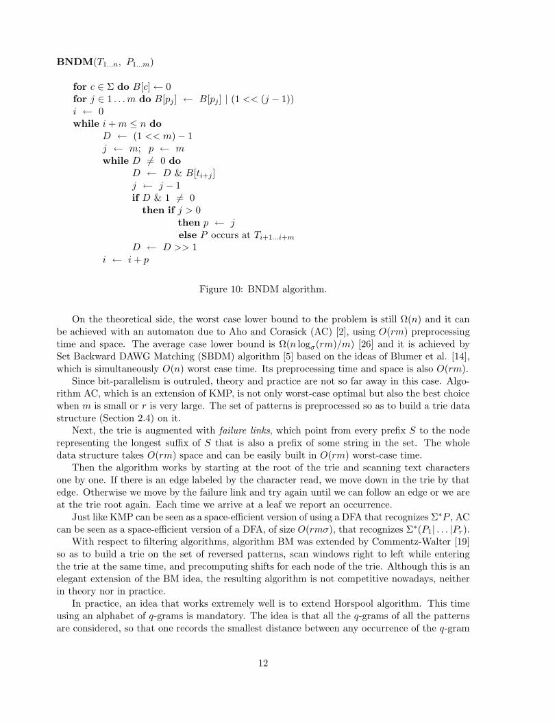
The first is Backward Nondeterministic DAWG Matching (BNDM) [57], by Navarro andRaffinot. The idea is to use the same BDM algorithm, but this time simulating the NFA withbit-parallelism instead of building the DFA. As can be seen in Figure 7, the structure of theNFA is rather regular and easy to simulate.

We work directly on P instead of reversing it. Hence the i-th bit of our bit mask D will beactive whenever state i− 1 in the NFA is active. We do not represent the initial state because itis active only in the beginning, to recognize the uninteresting empty substring of P . We buildtable B as before and initialize D = 111 . . . 1 (all 1’s). Hence, upon reading a new windowcharacter c, we update D as

D ←− D & B[c]

and at this point we can check a couple of conditions: (1) if D = 0 then the automaton hasdied; (2) if D & 1 = 1 then we have recognized a prefix of P . After this we prepare D for thenext window character by right-shifting:

D ←− D >> 1 .

BNDM is faster than BDM and actually the fastest algorithm for small alphabets and notvery short patterns (e.g., m ≥ 10 on DNA and m ≥ 30 on natural language). It is used inNavarro’s Nrgrep [52]. Its weakness, however, is that for long patterns we have to update manycomputer words to simulate it. This time the trick of updating only active computer words doesnot work because the active states distribute uniformly over the NFA. Hence the only practicalchoice is to search for P1...w and directly check potential occurrences. Figure 10 gives BNDMpseudocode.

Another practical alternative is algorithm Backward Oracle Matching (BOM) [4], by Allauzenet al., which replaces the suffix automaton by an oracle. The oracle is an automaton thatrecognizes more than the suffixes of P r. Therefore the algorithm makes shorter shifts. However,the fact that the oracle is simpler to build and smaller makes BOM faster in practice than BDM,and faster than BNDM for m ≥ 2w or so.

Construction of the oracle for a string S is rather simple compared to the deterministic suffixautomaton. It reminds the construction of the failure transitions for KMP. S is processed leftto right and for each new character c the path of failures is followed. At each step of the path,a new transition from the current node to the new final node, labeled by c, is inserted. In ourrunning example, the oracle is equal to the suffix automaton.

3.4 Searching for Multiple Patterns

Let us now assume that we want to search for a set of patterns P1 . . . Pr, all of length m forsimplicity of presentation. Several of the approaches designed to search for a single patterncan be extended. In particular, automata and filtering approaches can be gracefully extended.Bit-parallelism, on the other hand, is hardly useful because the resulting automata are ratherlarge, and hence even dividing the NFA update time by w is not enough.

11

BNDM(T1...n, P1...m)

for c ∈ Σ do B[c]← 0for j ∈ 1 . . . m do B[pj] ← B[pj] | (1 << (j − 1))i ← 0while i + m ≤ n do

D ← (1 << m)− 1j ← m; p ← mwhile D 6= 0 do

D ← D & B[ti+j]j ← j − 1if D & 1 6= 0

then if j > 0then p ← jelse P occurs at Ti+1...i+m

D ← D >> 1i ← i + p

Figure 10: BNDM algorithm.

On the theoretical side, the worst case lower bound to the problem is still Ω(n) and it canbe achieved with an automaton due to Aho and Corasick (AC) [2], using O(rm) preprocessingtime and space. The average case lower bound is Ω(n logσ(rm)/m) [26] and it is achieved bySet Backward DAWG Matching (SBDM) algorithm [5] based on the ideas of Blumer et al. [14],which is simultaneously O(n) worst case time. Its preprocessing time and space is also O(rm).

Since bit-parallelism is outruled, theory and practice are not so far away in this case. Algo-rithm AC, which is an extension of KMP, is not only worst-case optimal but also the best choicewhen m is small or r is very large. The set of patterns is preprocessed so as to build a trie datastructure (Section 2.4) on it.

Next, the trie is augmented with failure links, which point from every prefix S to the noderepresenting the longest suffix of S that is also a prefix of some string in the set. The wholedata structure takes O(rm) space and can be easily built in O(rm) worst-case time.

Then the algorithm works by starting at the root of the trie and scanning text charactersone by one. If there is an edge labeled by the character read, we move down in the trie by thatedge. Otherwise we move by the failure link and try again until we can follow an edge or we areat the trie root again. Each time we arrive at a leaf we report an occurrence.

Just like KMP can be seen as a space-efficient version of using a DFA that recognizes Σ∗P , ACcan be seen as a space-efficient version of a DFA, of size O(rmσ), that recognizes Σ∗(P1| . . . |Pr).

With respect to filtering algorithms, algorithm BM was extended by Commentz-Walter [19]so as to build a trie on the set of reversed patterns, scan windows right to left while enteringthe trie at the same time, and precomputing shifts for each node of the trie. Although this is anelegant extension of the BM idea, the resulting algorithm is not competitive nowadays, neitherin theory nor in practice.

In practice, an idea that works extremely well is to extend Horspool algorithm. This timeusing an alphabet of q-grams is mandatory. The idea is that all the q-grams of all the patternsare considered, so that one records the smallest distance between any occurrence of the q-gram

12

in any of the patterns, and the end of that pattern. The resulting algorithm (WM) [74], byWu and Manber, obtains average optimality by choosing q = logσ(rm), and is a very attractivechoice, because of its simplicity and efficiency. It is implemented in Agrep. Several practicalconsiderations are made in order to efficiently handling large alphabets. WM is in practice thefastest algorithm except when r is very large or σ is small.

With respect to merging automata and filtering, the average-optimal SBDM algorithm isan acceptable choice. It is based on the same idea of BDM, except that this time the suffixautomaton recognizes any suffix of any pattern. This automaton can be seen as the trie of thepatterns augmented with some extra edges that permit skipping pattern prefixes so as to godown directly to any trie node.

However, algorithm Set Backward Oracle Matching (SBOM) [5] by Allauzen and Raffinot,is simpler and faster. The idea is, again, to use an automaton that recognizes more than thesuffixes of the patterns. This benefits from simplicity and becomes faster than SBDM. Theconstruction of the oracle is very similar to that of the AC automaton and can be done inO(rm) space and time. SBOM is the best algorithm for small σ or very large r.

3.5 Searching for Complex Patterns

A more sophisticated form of searching permits patterns contain not only simple characters,but also “wild cards” of different types, such as (i) classes of characters like "[abc]" to match"a", "b" or "c"; (ii) optional characters or classes like "a?", where "a" may appear or not;and (iii) repeatable characters or classes like "a*", where "a" can appear zero or more times.These can be used to express other well known wild cards such as "." (which matches anycharacter), "*" (which stands for ".*"), bounded length gaps (such as any string of length 2 to4, which can be written as "...?.?"), etc. This can go as far as permitting the pattern to beany regular expression, that is, simple strings and any union, repetition and concatenation ofregular subexpressions.

As long as complex patterns are regular expressions, they can be converted into DFAs andsearched for in O(n) time [3]. This is theoretically appealing and, for sufficiently complexpatterns, the most practical choice. However, the preprocessing time and space requirementscan be exponential in m. Another alternative is to simulate the automata in nondeterministicform, obtaining O(mn) search time [65].

There are, however, particular cases where specialized solutions exist. On the theoreticalside, there exist solutions to search for patterns with classes of characters and simple wild cards[24, 60, 1]. Although theoretically interesting, these are not relevant in practice.

Bit-parallelism, on the other hand, yields extremely simple and efficient solutions to thiskind of problems. For example, classes of characters are easily handled in the Shift-And1 andBNDM algorithms. We only need to set the i-th bit B[c] for any c ∈ Pi.

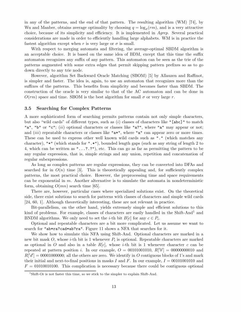
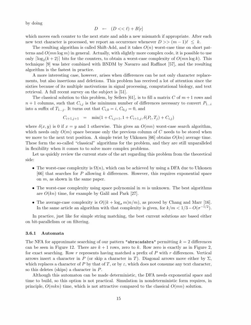
Optional and repeatable characters are a bit more complicated. Let us assume we want tosearch for "ab*ra?cad*ab?ra". Figure 11 shows a NFA that searches for it.

We show how to simulate this NFA using Shift-And. Optional characters are marked in anew bit mask O, whose i-th bit is 1 whenever Pi is optional. Repeatable characters are markedas optional in O and also in a table R[c], whose i-th bit is 1 whenever character c can berepeated at pattern position i. In our example, O = 00101001010, R[′b′] = 00000000010 andR[′d′] = 00001000000; all the others are zero. We identify in O contiguous blocks of 1’s and marktheir initial and next-to-final positions in masks I and F . In our example, I = 00101001010 andF = 01010010100. This complication is necessary because there could be contiguous optional

1Shift-Or is not faster this time, so we stick to the simpler to explain Shift-And.

13

a r a c d b r a

Σ

b a a0 1 2 3 4 5 6 7 8 9 1110

ε ε

b

ε ε

d

Figure 11: NFA that searches for "ab*ra?cad*ab?ra". The initial state is marked with “〉” andthe final state is double-circled.

characters. The update formula for mask D after reading text character c, when we permitoptional and repeatable characters, is as follows

D ← ((D << 1) | 1) & B[c]) | (D & R[c])

E ← D | FD ← D | (O & ((∼ (E − I)) ∧ E)) .

We do not attempt to explain all the details of this formula, but just to show that it is arather simple solution to a complex problem. It can be used for a Shift-And-like scanning ofthe text or for a BNDM-like search. In this latter case, the window length should be that ofthe shortest possible occurrence of P , and when we arrive at the beginning of the window, thepresence of an occurrence is not guaranteed. Rather, if we have found a pattern prefix at thebeginning of the window, we should verify whether an occurrence starts at that position. Thisis done by simulating an automaton like that of Figure 11 with the initial self-loop removed.

In general, worst-case search time is O(n) for short patterns and O(nm/w) for longer onesusing bit-parallelism. A BNDM-like solution can be much faster depending on the sizes of theclasses and number of optional and repeatable characters. In practice, these solutions are simpleand practical, and they have been implemented in nrgrep [52].

Full regular expressions are more resistant to simple approaches. Several lines of attack havebeen tried, both classical and bit-parallel, to obtain a tradeoff between search time and space.Both have converged to O(mn/ log s) time using O(s) space [50, 56].

Finally, efficient searching for multiple complex patterns is an open problem.

3.6 Approximate Pattern Matching

An extremely useful search option in text retrieval systems is to allow a limited number k,of differences between pattern P and its occurrences in T . The search problem varies widelydepending on what is considered a “difference”.

A simple choice is to assume that a difference is a substitution of one character by another.Therefore, we are permitted to change up to k letters in P in order to match it in a textposition. This problem can be nicely solved using bit-parallelism, and it was in fact one of thefirst extensions to Shift-Or, by Baeza-Yates and Gonnet, showing the potential of the approach[9].

Let us reconsider the NFA of Figure 2. After having read text position j, state i is activewhenever P1...i matches Tj−i+1...j. This time, let us consider that each state i is not simply activeor inactive, but that it remembers how many characters differ between P1...i and Tj−i+1...j. Everytime the counter at state m does not exceed k, we have an occurrence with at most k mismatches.

Our bit mask D holds m counters, cm . . . c1, for each of which we have to reserve ℓ =⌈log2(m + 1)⌉ bits. We precompute a bit mask table of counters B[c], whose i-th counter willbe 0 if Pi = c and 1 otherwise. Hence, after reading text character c we can update D simply

14

by doingD ← (D << ℓ) + B[c]

which moves each counter to the next state and adds a new mismatch if appropriate. After eachnew text character is processed, we report an occurrence whenever D >> (m− 1)ℓ ≤ k.

The resulting algorithm is called Shift-Add, and it takes O(n) worst-case time on short pat-terns and O(mn log m) in general. Actually, with slightly more complex code, it is possible to useonly ⌈log2(k + 2)⌉ bits for the counters, to obtain a worst-case complexity of O(mn log k). Thistechnique [9] was later combined with BNDM by Navarro and Raffinot [57], and the resultingalgorithm is the fastest in practice.

A more interesting case, however, arises when differences can be not only character replace-ments, but also insertions and deletions. This problem has received a lot of attention since thesixties because of its multiple motivations in signal processing, computational biology, and textretrieval. A full recent survey on the subject is [51].

The classical solution to this problem, by Sellers [61], is to fill a matrix C of m + 1 rows andn + 1 columns, such that Ci,j is the minimum number of differences necessary to convert P1...i

into a suffix of T1...j . It turns out that Ci,0 = i, C0,j = 0, and

Ci+1,j+1 = min(1 + Ci,j+1, 1 + Ci+1,j, δ(Pi, Tj) + Ci,j)

where δ(x, y) is 0 if x = y and 1 otherwise. This gives an O(mn) worst-case search algorithm,which needs only O(m) space because only the previous column of C needs to be stored whenwe move to the next text position. A simple twist by Ukkonen [66] obtains O(kn) average time.These form the so-called “classical” algorithms for the problem, and they are still unparalleledin flexibility when it comes to to solve more complex problems.

Let us quickly review the current state of the art regarding this problem from the theoreticalside:

• The worst-case complexity is Ω(n), which can be achieved by using a DFA due to Ukkonen[66] that searches for P allowing k differences. However, this requires exponential spaceon m, as shown in the same paper.

• The worst-case complexity using space polynomial in m is unknown. The best algorithmsare O(kn) time, for example by Galil and Park [27].

• The average-case complexity is O((k + logσ m)n/m), as proved by Chang and Marr [16].In the same article an algorithm with that complexity is given, for k/m < 1/3−O(σ−1/2).

In practice, just like for simple string matching, the best current solutions are based eitheron bit-parallelism or on filtering.

3.6.1 Automata

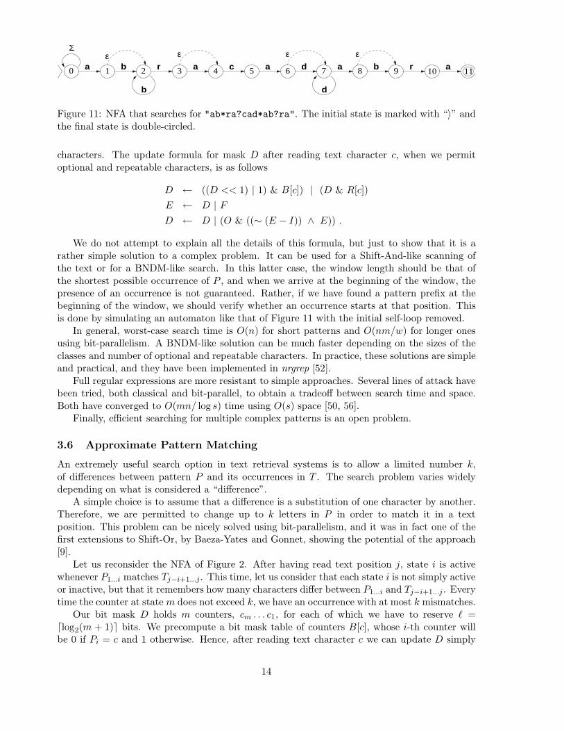
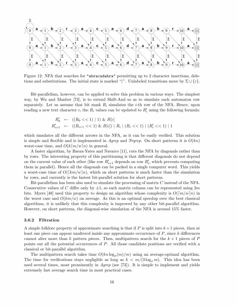
The NFA for approximate searching of our pattern "abracadabra" permitting k = 2 differencescan be seen in Figure 12. There are k + 1 rows, zero to k. Row zero is exactly as in Figure 2,for exact searching. Row r represents having matched a prefix of P with r differences. Verticalarrows insert a character in P (or skip a character in T ). Diagonal arrows move either by Σ,which replaces a character of P by that of T , or by ε, which does not consume any text character,so this deletes (skips) a character in P .

Although this automaton can be made deterministic, the DFA needs exponential space andtime to build, so this option is not practical. Simulation in nondeterministic form requires, inprinciple, O(mkn) time, which is not attractive compared to the classical O(mn) solution.

15

a r a c d b r ab a a0 1 2 3 4 5 6 7 8 9 1110

a r a c d b r ab a a0 1 2 3 4 5 6 7 8 9 1110

a r a c d b r a

Σ

b a a0 1 2 3 4 5 6 7 8 9 1110

Σ

Σ Σ Σ Σ Σ Σ

Σ Σ Σ Σ Σ Σ

Σ Σ Σ Σ Σ Σ

Σ Σ Σ Σ Σ

Figure 12: NFA that searches for "abracadabra" permitting up to 2 character insertions, dele-tions and substitutions. The initial state is marked “〉”. Unlabeled transitions move by Σ∪ε.

Bit-parallelism, however, can be applied to solve this problem in various ways. The simplestway, by Wu and Manber [73], is to extend Shift-And so as to simulate each automaton rowseparately. Let us assume that bit mask Ri simulates the i-th row of the NFA. Hence, uponreading a new text character c, the Ri values can be updated to R′

i using the following formula:

R′

0 ← ((R0 << 1) | 1) & B[c]

R′

i+1 ← ((Ri+1 << 1) & B[c]) | Ri | (Ri << 1) | (R′

i << 1) | 1

which simulates all the different arrows in the NFA, as it can be easily verified. This solutionis simple and flexible and is implemented in Agrep and Nrgrep. On short patterns it is O(kn)worst-case time, and O(k⌈m/w⌉n) in general.

A faster algorithm, by Baeza-Yates and Navarro [11], cuts the NFA by diagonals rather thanby rows. The interesting property of this partitioning is that different diagonals do not dependon the current value of each other (like row R′

i+1 depends on row R′

i, which prevents computingthem in parallel). Hence all the diagonals can be packed in a single computer word. This yieldsa worst-case time of O(⌈km/w⌉n), which on short patterns is much faster than the simulationby rows, and currently is the fastest bit-parallel solution for short patterns.

Bit-parallelism has been also used to simulate the processing of matrix C instead of the NFA.Consecutive values of C differ only by ±1, so each matrix column can be represented using 2mbits. Myers [48] used this property to design an algorithm whose complexity is O(⌈m/w⌉n) inthe worst case and O(km/w) on average. As this is an optimal speedup over the best classicalalgorithms, it is unlikely that this complexity is improved by any other bit-parallel algorithm.However, on short patterns, the diagonal-wise simulation of the NFA is around 15% faster.

3.6.2 Filtration

A simple folklore property of approximate searching is that if P is split into k+1 pieces, then atleast one piece can appear unaltered inside any approximate occurrence of P , since k differencescannot alter more than k pattern pieces. Then, multipattern search for the k + 1 pieces of Ppoints out all the potential occurrences of P . All those candidate positions are verified with aclassical or bit-parallel algorithm.

The multipattern search takes time O(kn logσ(m)/m) using an average-optimal algorithm.The time for verifications stays negligible as long as k < m/(3 logσ m). This idea has beenused several times, most prominently in Agrep (see [73]). It is simple to implement and yieldsextremely fast average search time in most practical cases.

16

However, the above algorithm has a limit of applicability that prevents using it when k/mbecomes too large. Moreover, this limit is narrower for smaller σ. This is, for example, the casein several computational biology applications. In this case, the optimal algorithm by Changand Marr [16] becomes a practical choice. It can be used up to k/m < 1/3−O(σ−1/2) and hasoptimal average complexity (however, it is not as fast as partition into k + 1 pieces when thelatter can be applied). Their idea is an improvement of previous algorithms that use q-grams(for example [69]).

This algorithm works as follows. The text is divided into consecutive blocks of length (m−k)/2. Since any occurrence of P is of length at least m− k, any occurrence contains at least onecomplete block. A number q is chosen, in a way that will be made clear soon.

The preprocessing of P consists in computing, for every string S of length q, the minimumnumber of differences needed to find S inside P . Preprocessing time is O(mσq) and space isO(σq).

The search stage proceeds as follows. For each text block Z, its consecutive q-grams Z1...q,Zq+1...2q, . . . are read one by one, and their minimum differences to match them inside P areaccumulated. This is continued until (i) the accumulated differences exceed k, in which case thecurrent block cannot be contained in an occurrence, and we can go on to the next block; (ii) wereach the end of the block, in which case the block is verified.

It is shown that on average one examines O(k/q+1) q-grams per block, so O(k+q) charactersare examined. On the other hand, q must be Ω(logσ m) so that the probability of verifying ablock is low enough. This yields overall time O((k + logσ m)n/m) for k/m < 1/3 − O(σ−1/2),with space polynomial in m.

For the same limit on k/m, another practical algorithm is obtained by combining a bit-parallel algorithm with a BNDM scheme, as done by Navarro and Raffinot [57] and Hyyro andNavarro [37]. For higher k/m ratios, no good filtering algorithm exists, and the only choice isto resort to classical or pure bit-parallel algorithms.

3.6.3 Extensions

Recently, the average-optimal results for approximate string matching were extended to search-ing for r patterns by Fredriksson and Navarro [26]. They showed that the average complexityof the problem is O((k + logσ(rm))n/m), and obtained an algorithm achieving that complex-ity. This is similar to the algorithm for one pattern, except that q-grams are preprocessed soas to find their minimum number of differences across all the patterns in the set. This timeq = Θ(logσ(rm)). They showed that the result is useful in practice.

The other choice to address this problem is to partition each pattern in the set into k +1 pieces and search for the r(k + 1) pieces in the set, verifying each piece occurrence for acomplete occurrence of the patterns containing the piece. The search time is not optimal,O(kn logσ(rm)/m), but it is the best in practice for low k/m values.

Approximate searching of complex pattern has been addressed by Navarro in Nrgrep, bycombining Shift-And and BNDM with the row-wise simulation of the NFA that recognizes P .Each row of the NFA now recognizes a complex pattern P .

Finally, approximate searching of regular expressions can be done in O(mn) time and O(m)space, as shown by Myers and Miller [49], and in general in O(mn/ log s) time using O(s) space,as shown by Wu et al. and Navarro [75, 53].

17

4 Indexed Text Searching

In this section we review the main techniques to maintain an index over the text, to speed upsearches. As explained, the text must be sufficiently static (few or no changes over time) to justifyindexing, as maintaining an index is costly compared to a single search. The best candidatesfor indexing are fully static texts such as historical data and dictionaries, but indexing is alsoapplied to rather more dynamic data like the Web due to its large volume.

4.1 Index Points

In sequential searching we assumed that the user wanted to find any substring of the text. Thiswas because the algorithms are not radically different if this is not the case. However, indexingschemes depend much more on the retrieval model, so we pay some attention to the issue now.

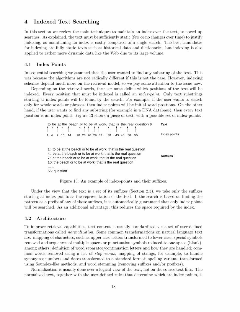
Depending on the retrieval needs, the user must define which positions of the text will beindexed. Every position that must be indexed is called an index-point. Only text substringsstarting at index points will be found by the search. For example, if the user wants to searchonly for whole words or phrases, then index points will be initial word positions. On the otherhand, if the user wants to find any substring (for example in a DNA database), then every textposition is an index point. Figure 13 shows a piece of text, with a possible set of index-points.

1 4 7 10 14 29 38 43 46 50 5532262320

to be at the beach or to be at work, that is the real question $

1: to be at the beach or to be at work, that is the real question4: be at the beach or to be at work, that is the real question7: at the beach or to be at work, that is the real question10: the beach or to be at work, that is the real question......55: question

Suffixes

Index points

Text

Figure 13: An example of index-points and their suffixes.

Under the view that the text is a set of its suffixes (Section 2.3), we take only the suffixesstarting at index points as the representation of the text. If the search is based on finding thepattern as a prefix of any of those suffixes, it is automatically guaranteed that only index pointswill be searched. As an additional advantage, this reduces the space required by the index.

4.2 Architecture

To improve retrieval capabilities, text content is usually standardized via a set of user-definedtransformations called normalization. Some common transformations on natural language textare: mapping of characters, such as upper case letters transformed to lower case; special symbolsremoved and sequences of multiple spaces or punctuation symbols reduced to one space (blank),among others; definition of word separator/continuation letters and how they are handled; com-mon words removed using a list of stop words; mapping of strings, for example, to handlesynonyms; numbers and dates transformed to a standard format; spelling variants transformedusing Soundex-like methods; and word stemming (removing suffixes and/or prefixes).

Normalization is usually done over a logical view of the text, not on the source text files. Thenormalized text, together with the user-defined rules that determine which are index points, is

18

used to build the index.The search pattern must also be normalized before searching the index for it. Once the text

search engine retrieves the set of text positions that match the pattern, the original text is usedto feed the user interface with the information that must be visualized.

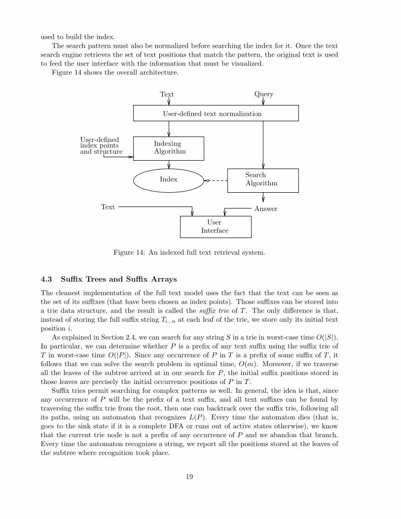
Figure 14 shows the overall architecture.

Index

User-defined text normalization

Query

Answer

Text

User-definedindex pointsand structure

IndexingAlgorithm

SearchAlgorithm

Text

InterfaceUser

Figure 14: An indexed full text retrieval system.

4.3 Suffix Trees and Suffix Arrays

The cleanest implementation of the full text model uses the fact that the text can be seen asthe set of its suffixes (that have been chosen as index points). Those suffixes can be stored intoa trie data structure, and the result is called the suffix trie of T . The only difference is that,instead of storing the full suffix string Ti...n at each leaf of the trie, we store only its initial textposition i.

As explained in Section 2.4, we can search for any string S in a trie in worst-case time O(|S|).In particular, we can determine whether P is a prefix of any text suffix using the suffix trie ofT in worst-case time O(|P |). Since any occurrence of P in T is a prefix of some suffix of T , itfollows that we can solve the search problem in optimal time, O(m). Moreover, if we traverseall the leaves of the subtree arrived at in our search for P , the initial suffix positions stored inthose leaves are precisely the initial occurrence positions of P in T .

Suffix tries permit searching for complex patterns as well. In general, the idea is that, sinceany occurrence of P will be the prefix of a text suffix, and all text suffixes can be found bytraversing the suffix trie from the root, then one can backtrack over the suffix trie, following allits paths, using an automaton that recognizes L(P ). Every time the automaton dies (that is,goes to the sink state if it is a complete DFA or runs out of active states otherwise), we knowthat the current trie node is not a prefix of any occurrence of P and we abandon that branch.Every time the automaton recognizes a string, we report all the positions stored at the leaves ofthe subtree where recognition took place.

19

This algorithm is general and works in sublinear time (that is, o(n)) in most cases. Forgeneral regular expressions, the number of nodes traversed is O(nλ), where 0 ≤ λ ≤ 1 dependson the structure of the regular expression, as shown by Baeza-Yates and Gonnet [10]. Forapproximate searching the time is exponential in k, as shown by Ukkonen [68], and it can bedone O(nλ) again by appropriately partitioning the pattern into pieces, as shown by Navarroand Baeza-Yates [54]. This time λ will be smaller than 1 if k/m < 1 − e/

√σ. Other types of

sophisticated searches have been considered [43, 6, 34, 31].The only problem with this approach is that the suffix trie may be rather large compared

to the text. In the worst case, it can be of size O(n2), although on average it is of size O(n).To ensure O(n) size in the worst case, any unary path in the suffix trie is compacted into asingle edge. Edges now will be labeled by a string, not only a character. There are several waysto represent the string labeling those edges in constant space. One is a couple of pointers tothe text, since those strings are text substrings. Another is to simply store its first characterand length, so the search skips some characters of P , which must be verified at the end againstTi...i+m−1, where i is the text position at any leaf in the answer. Since the resulting tree hasdegree at least two and it has O(n) leaves (text suffixes) it follows that it is O(n) size in theworst case. The result, due to Weiner [70], is called a suffix tree [6, 31].

Suffix trees can be built in optimal O(n) worst-case time, as shown by McCreight and others[46, 67, 29], and can simulate any algorithm over suffix tries with the same complexity. So inpractice they are preferred over suffix tries, although it is much easier to think of algorithmsover the suffix trie and then implement them over the suffix tree.

Still, suffix trees are unsatisfactory in most practical applications. The constant that mul-tiplies their O(n) space complexity is large. Naively implemented, suffix trees require at least20 bytes per index point (this can be as bad as 20 times the text size). Even the most space-efficient implementations, by Giegerich et al. [30], takes 9 to 12 bytes per index point. Moreover,its construction accesses memory at random, so it cannot be efficiently built (nor searched) insecondary memory. There exist other related data structures such as Blumer et al.’s DAWG(an automaton that recognizes all the text substrings, which can be obtained by minimizingthe suffix trie) [22], and Crochemore and Verin’s Compact DAWG (the result of minimizing thesuffix tree) [23].

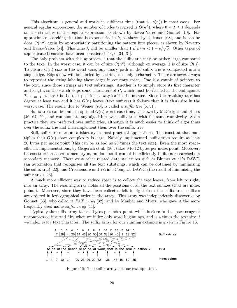
A much more efficient way to reduce space is to collect the tree leaves, from left to right,into an array. The resulting array holds all the positions of all the text suffixes (that are indexpoints). Moreover, since they have been collected left to right from the suffix tree, suffixesare ordered in lexicographical order in the array. This array was independently discovered byGonnet [33], who called it PAT array [32], and by Manber and Myers, who gave it the morefrequently used name suffix array [44].

Typically the suffix array takes 4 bytes per index point, which is close to the space usage ofuncompressed inverted files when we index only word beginnings, and is 4 times the text size ifwe index every text character. The suffix array for our running example is given in Figure 15.

7 29 4 26 14 43 20 55 50 38 10 46 1 32231 2 3 4 5 6 7 8 9 10 11 12 13 14 15

to be at the beach or to be at work, that is the real question $

Index points

Text

1 4 7 10 14 29 38 43 46 50 5532262320

Suffix Array

Figure 15: The suffix array for our example text.

20

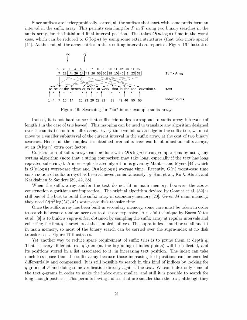
Since suffixes are lexicographically sorted, all the suffixes that start with some prefix form aninterval in the suffix array. This permits searching for P in T using two binary searches in thesuffix array, for the initial and final interval position. This takes O(m log n) time in the worstcase, which can be reduced to O(log n) by using some extra structures (that take more space)[44]. At the end, all the array entries in the resulting interval are reported. Figure 16 illustrates.

1 2 3 4 5 6 7 8 9 10 11 12 13 14 15

to be at the beach or to be at work, that is the real question $

Index points

Text

1 4 7 10 14 29 38 43 46 50 5532262320

Suffix Array

be bf

7 29 4 26 14 43 20 55 50 38 10 46 1 3223

Figure 16: Searching for "be" in our example suffix array.

Indeed, it is not hard to see that suffix trie nodes correspond to suffix array intervals (oflength 1 in the case of trie leaves). This mapping can be used to translate any algorithm designedover the suffix trie onto a suffix array. Every time we follow an edge in the suffix trie, we mustmove to a smaller subinterval of the current interval in the suffix array, at the cost of two binarysearches. Hence, all the complexities obtained over suffix trees can be obtained on suffix arrays,at an O(log n) extra cost factor.

Construction of suffix arrays can be done with O(n log n) string comparisons by using anysorting algorithm (note that a string comparison may take long, especially if the text has longrepeated substrings). A more sophisticated algorithm is given by Manber and Myers [44], whichis O(n log n) worst-case time and O(n log log n) average time. Recently, O(n) worst-case timeconstruction of suffix arrays has been achieved, simultaneously by Kim et al., Ko & Aluru, andKarkkainen & Sanders [39, 42, 38].

When the suffix array and/or the text do not fit in main memory, however, the aboveconstruction algorithms are impractical. The original algorithm devised by Gonnet et al. [32] isstill one of the best to build the suffix array in secondary memory [20]. Given M main memory,they need O(n2 log(M)/M) worst-case disk transfer time.

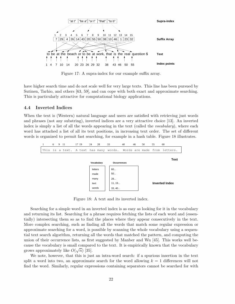
Once the suffix array has been built in secondary memory, some care must be taken in orderto search it because random accesses to disk are expensive. A useful technique by Baeza-Yateset al. [8] is to build a supra-index, obtained by sampling the suffix array at regular intervals andcollecting the first q characters of the sampled suffixes. The supra-index should be small and fitin main memory, so most of the binary search can be carried over the supra-index at no disktransfer cost. Figure 17 illustrates.

Yet another way to reduce space requirement of suffix tries is to prune them at depth q.That is, every different text q-gram (at the beginning of index points) will be collected, andits positions stored in a list associated to it, in increasing text position. The index can takemuch less space than the suffix array because those increasing text positions can be encodeddifferentially and compressed. It is still possible to search in this kind of indices by looking forq-grams of P and doing some verification directly against the text. We can index only some ofthe text q-grams in order to make the index even smaller, and still it is possible to search forlong enough patterns. This permits having indices that are smaller than the text, although they

21

7 29 4 26 14 43 20 55 50 38 10 46 1 32231 2 3 4 5 6 7 8 9 10 11 12 13 14 15

"at t" "be a" "or t" "to b""that"

to be at the beach or to be at work, that is the real question $

Index points

Text

1 4 7 10 14 29 38 43 46 50 5532262320

Suffix Array

Supra-index

Figure 17: A supra-index for our example suffix array.

have higher search time and do not scale well for very large texts. This line has been pursued bySutinen, Tarhio, and others [63, 59], and can cope with both exact and approximate searching.This is particularly attractive for computational biology applications.

4.4 Inverted Indices

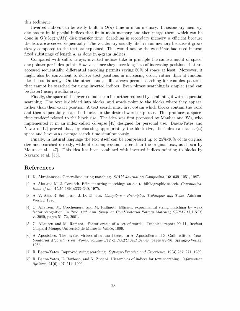
When the text is (Western) natural language and users are satisfied with retrieving just wordsand phrases (not any substring), inverted indices are a very attractive choice [13]. An invertedindex is simply a list of all the words appearing in the text (called the vocabulary), where eachword has attached a list of all its text positions, in increasing text order. The set of differentwords is organized to permit fast searching, for example in a hash table. Figure 18 illustrates.

words

text

many

made

letters

33, 40...

11, 19...

60...

50...

28...

Vocabulary Occurrences

This is a text. A text has many words. Words are made from letters.

1 6 9 11 17 19 24 28 33 40 46 50 55 60

Text

Inverted Index

Figure 18: A text and its inverted index.

Searching for a simple word in an inverted index is as easy as looking for it in the vocabularyand returning its list. Searching for a phrase requires fetching the lists of each word and (essen-tially) intersecting them so as to find the places where they appear consecutively in the text.More complex searching, such as finding all the words that match some regular expression orapproximate searching for a word, is possible by scanning the whole vocabulary using a sequen-tial text search algorithm, returning all the words that matched the pattern, and computing theunion of their occurrence lists, as first suggested by Manber and Wu [45]. This works well be-cause the vocabulary is small compared to the text. It is empirically known that the vocabularygrows approximately like O(

√n) [35].

We note, however, that this is just an intra-word search: if a spurious insertion in the textsplit a word into two, an approximate search for the word allowing k = 1 differences will notfind the word. Similarly, regular expressions containing separators cannot be searched for with

22

this technique.Inverted indices can be easily built in O(n) time in main memory. In secondary memory,

one has to build partial indices that fit in main memory and then merge them, which can bedone in O(n log(n/M)) disk transfer time. Searching in secondary memory is efficient becausethe lists are accessed sequentially. The vocabulary usually fits in main memory because it growsslowly compared to the text, as explained. This would not be the case if we had used insteadfixed substrings of length q, as done in q-gram indices.

Compared with suffix arrays, inverted indices take in principle the same amount of space:one pointer per index point. However, since they store long lists of increasing positions that areaccessed sequentially, differential encoding permits saving 50% of space at least. Moreover, itmight also be convenient to deliver text positions in increasing order, rather than at randomlike the suffix array. On the other hand, suffix arrays permit searching for complex patternsthat cannot be searched for using inverted indices. Even phrase searching is simpler (and canbe faster) using a suffix array.

Finally, the space of the inverted index can be further reduced by combining it with sequentialsearching. The text is divided into blocks, and words point to the blocks where they appear,rather than their exact position. A text search must first obtain which blocks contain the wordand then sequentially scan the blocks for the desired word or phrase. This produces a space-time tradeoff related to the block size. The idea was first proposed by Manber and Wu, whoimplemented it in an index called Glimpse [45] designed for personal use. Baeza-Yates andNavarro [12] proved that, by choosing appropriately the block size, the index can take o(n)space and have o(n) average search time simultaneously.

Finally, in natural language the text itself can be compressed up to 25%-30% of its originalsize and searched directly, without decompression, faster than the original text, as shown byMoura et al. [47]. This idea has been combined with inverted indices pointing to blocks byNavarro et al. [55].

References

[1] K. Abrahamson. Generalized string matching. SIAM Journal on Computing, 16:1039–1051, 1987.

[2] A. Aho and M. J. Corasick. Efficient string matching: an aid to bibliographic search. Communica-tions of the ACM, 18(6):333–340, 1975.

[3] A. V. Aho, R. Sethi, and J. D. Ullman. Compilers – Principles, Techniques and Tools. Addison-Wesley, 1986.

[4] C. Allauzen, M. Crochemore, and M. Raffinot. Efficient experimental string matching by weakfactor recognition. In Proc. 12th Ann. Symp. on Combinatorial Pattern Matching (CPM’01), LNCSv. 2089, pages 51–72, 2001.

[5] C. Allauzen and M. Raffinot. Factor oracle of a set of words. Technical report 99–11, InstitutGaspard-Monge, Universite de Marne-la-Vallee, 1999.

[6] A. Apostolico. The myriad virtues of subword trees. In A. Apostolico and Z. Galil, editors, Com-binatorial Algorithms on Words, volume F12 of NATO ASI Series, pages 85–96. Springer-Verlag,1985.

[7] R. Baeza-Yates. Improved string searching. Software-Practice and Experience, 19(3):257–271, 1989.

[8] R. Baeza-Yates, E. Barbosa, and N. Ziviani. Hierarchies of indices for text searching. InformationSystems, 21(6):497–514, 1996.

23

[9] R. Baeza-Yates and G. Gonnet. A new approach to text searching. In Proc. 12th Ann. Int. ACMConf. on Research and Development in Information Retrieval (SIGIR’89), pages 168–175, 1989.(Addendum in ACM SIGIR Forum, V. 23, Numbers 3, 4, 1989, page 7.).

[10] R. Baeza-Yates and G. H. Gonnet. Fast text searching for regular expressions or automaton searchingon tries. Journal of the ACM, 43(6):915–936, 1996.

[11] R. Baeza-Yates and G. Navarro. Faster approximate string matching. Algorithmica, 23(2):127–158,1999.

[12] R. Baeza-Yates and G. Navarro. Block-addressing indices for approximate text retrieval. Journal ofthe American Society for Information Science, 51(1):69–82, 2000.

[13] R. Baeza-Yates and B. Ribeiro-Neto. Modern Information Retrieval. Addison-Wesley, 1999.

[14] A. Blumer, J. Blumer, A. Ehrenfeucht, D. Haussler, and R. McConnel. Complete inverted files forefficient text retrieval and analysis. Journal of the ACM, 34(3):578–595, 1987.

[15] R. Boyer and S. Moore. A fast string searching algorithm. Communications of the ACM, 20:762–772,1977.

[16] W. Chang and T. Marr. Approximate string matching with local similarity. In Proc. 5th Ann. Symp.on Combinatorial Pattern Matching (CPM’94), LNCS v. 807, pages 259–273, 1994.

[17] R. Cole. Tight bounds on the complexity of the Boyer-Moore string matching algorithm. In Proc.2nd ACM-SIAM Ann. Symp. on Discrete Algorithms (SODA’91), pages 224–233, 1991.

[18] L. Colussi, Z. Galil, and R. Giancarlo. The exact complexity of string matching. In Proc. 31st IEEEAnn. Symp. on Foundations of Computer Science, volume 1, pages 135–143, 1990.

[19] B. Commentz-Walter. A string matching algorithm fast on the average. In Proc. 6th Int. Coll. onAutomata, Languages and Programming (ICALP’79), LNCS v. 71, pages 118–132, 1979.

[20] A. Crauser and P. Ferragina. On constructing suffix arrays in external memory. Algorithmica,32(1):1–35, 2002.

[21] M. Crochemore, A. Czumaj, L. Gasieniec, S. Jarominek, T. Lecroq, W. Plandowski, and W. Rytter.Speeding up two string matching algorithms. Algorithmica, 12(4/5):247–267, 1994.

[22] M. Crochemore and W. Rytter. Text Algorithms. Oxford University Press, 1994.

[23] M. Crochemore and R. Verin. Direct construction of compact directed acyclic word graphs. InProc. 8th Annual Symposium on Combinatorial Pattern Matching (CPM’97), LNCS v. 1264, pages116–129, 1997.

[24] M. Fischer and M. Paterson. String matching and other products. In Proc. 7th SIAM-AMS Com-plexity of Computation, pages 113–125. American Mathematical Society, 1974.

[25] W. Frakes and R. Baeza-Yates, editors. Information Retrieval: Data Structures and Algorithms.Prentice-Hall, 1992.

[26] K. Fredriksson and G. Navarro. Average-optimal multiple approximate string matching. In Proc.14th Ann. Symp. on Combinatorial Pattern Matching (CPM’03), LNCS v. 2676, pages 109–128,2003.

[27] Z. Galil and K. Park. An improved algorithm for approximate string matching. SIAM Journal ofComputing, 19(6):989–999, 1990.

[28] Z. Galil and J. Seiferas. Linear–time string matching using only a fixed number of local storagelocations. Theoretical Computer Science, 13:331–336, 1981.

[29] R. Giegerich and S. Kurtz. From ukkonen to mccreight and weiner: A unifying view of linear-timesuffix tree construction. Algorithmica, 19(3):331–353, 1997.

24

[30] R. Giegerich, S. Kurtz, and J. Stoye. Efficient implementation of lazy suffix trees. In Proc. 3rdWorkshop on Algorithm Engineering (WAE’99), LNCS v. 1668, pages 30–42, 1999.

[31] G. Gonnet and R. Baeza-Yates. Handbook of Algorithms and Data Structures – In Pascal and C.Addison-Wesley, 2nd edition, 1991.

[32] G. Gonnet, R. Baeza-Yates, and T. Snider. New indices for text: Pat trees and pat arrays. InW. Frakes and R. Baeza-Yates, editors, Information Retrieval: Algorithms and Data Structures,chapter 5, pages 66–82. Prentice-Hall, 1992.

[33] G.H. Gonnet. PAT 3.1: An efficient text searching system, User’s manual. UW Centre for the NewOED, University of Waterloo, 1987.

[34] D. Gusfield. Algorithms on Strings, Trees, and Sequences. Cambridge University Press, 1997.

[35] H. Heaps. Information Retrieval: Computational and Theoretical Aspects. Academic Press, 1978.

[36] R. Horspool. Practical fast searching in strings. Software Practice and Experience, 10(6):501–506,1980.

[37] H. Hyyro and G. Navarro. Faster bit-parallel approximate string matching. In Proc. 13th AnnualSymposium on Combinatorial Pattern Matching (CPM’02), LNCS 2373, pages 203–224, 2002.

[38] J. Karkkainen and P. Sanders. Simple linear work suffix array construction. In ICALP, to appear,2003.

[39] D. Kim, J. Sim, H. Park, and K. Park. Linear-time construction of suffix arrays. In Proc. 14th Ann.Symp. on Combinatorial Pattern Matching (CPM’03), LNCS v. 2676, pages 186–199, 2003.

[40] J. Kim and J. Shawe-Taylor. Fast string matching using an n-gram algorithm. University of London,1991.

[41] D. Knuth, J. Morris, and V. Pratt. Fast pattern matching in strings. SIAM Journal on Computing,6:323–350, 1977.

[42] P. Ko and S. Aluru. Space efficient linear time construction of suffix arrays. In Proc. 14th Ann.Symp. on Combinatorial Pattern Matching (CPM’03), LNCS v. 2676, pages 200–210, 2003.

[43] U. Manber and R. A. Baeza-Yates. An algorithm for string matching with a sequence of don’t cares.Information Processing Letters, 37(3):133–136, 1991.

[44] U. Manber and E. W. Myers. Suffix arrays: a new method for on-line string searches. SIAM Journalon Computing, 22(5):935–948, 1993.

[45] U. Manber and S. Wu. Glimpse: A tool to search through entire file systems. In Proc. USENIXTechnical Conference, pages 23–32. USENIX Association, Berkeley, CA, USA, Winter 1994.

[46] E. M. McCreight. A space-economical suffix tree construction algorithm. Journal of Algorithms,23(2):262–272, 1976.

[47] E. Moura, G. Navarro, N. Ziviani, and R. Baeza-Yates. Fast and flexible word searching on com-pressed text. ACM Transactions on Information Systems, 18(2):113–139, 2000.

[48] E. Myers. A fast bit-vector algorithm for approximate string matching based on dynamic program-ming. Journal of the ACM, 46(3):395–415, 1999.

[49] E. Myers and W. Miller. Approximate matching of regular expressions. Bulletin of MathematicalBiology, 51(1):5–37, 1989.

[50] E. W. Myers. A four russians algorithm for regular expression pattern matching. Journal of theACM, 39(2):430–448, 1992.

[51] G. Navarro. A guided tour to approximate string matching. ACM Computing Surveys, 33(1):31–88,2001.

25

[52] G. Navarro. Nr-grep: a fast and flexible pattern matching tool. Software Practice and Experience,31:1265–1312, 2001.

[53] G. Navarro. Approximate regular expression searching with arbitrary integer weights. TechnicalReport TR/DCC-2002-6, Department of Computer Science, University of Chile, July 2002.

[54] G. Navarro and R. Baeza-Yates. A hybrid indexing method for approximate string matching. Journalof Discrete Algorithms, 1(1):205–239, 2000.

[55] G. Navarro, E. Moura, M. Neubert, N. Ziviani, and R. Baeza-Yates. Adding compression to blockaddressing inverted indexes. Information Retrieval, 3(1):49–77, 2000.

[56] G. Navarro and M. Raffinot. Fast regular expression search. In Proc. 3rd Workshop on AlgorithmEngineering (WAE’99), LNCS v. 1668, pages 199–213, 1999.

[57] G. Navarro and M. Raffinot. Fast and flexible string matching by combining bit-parallelism andsuffix automata. ACM Journal of Experimental Algorithmics, 5(4), 2000.

[58] G. Navarro and M. Raffinot. Flexible Pattern Matching in Strings – Practical on-line search algo-rithms for texts and biological sequences. Cambridge University Press, 2002.

[59] G. Navarro, E. Sutinen, J. Tanninen, and J. Tarhio. Indexing text with approximate q-grams. InProc. 11th Annual Symposium on Combinatorial Pattern Matching (CPM’2000), LNCS v. 1848,pages 350–363, 2000.

[60] R. Pinter. Efficient string matching with don’t-care patterns. In A. Apostolico and Z. Galil, editors,Combinatorial Algorithms on Words, volume F12 of NATO ASI Series, pages 11–29. Springer-Verlag,1985.

[61] P. Sellers. The theory and computation of evolutionary distances: Pattern recognition. Journal ofAlgorithms, 1:359–373, 1980.

[62] D. Sunday. A very fast substring search algorithm. Communications of the ACM, 33(8):132–142,1990.

[63] E. Sutinen and J. Tarhio. Filtration with q-samples in approximate string matching. In Proc. 7thAnnual Symposium on Combinatorial Pattern Matching (CPM’96), LNCS v. 1075, pages 50–61,1996.

[64] J. Tarhio and H. Peltola. String matching in the DNA alphabet. Software Practice and Experience,27(7):851–861, 1997.

[65] K. Thompson. Regular expression search algorithm. Communications of the ACM, 11:419–422,1968.

[66] E. Ukkonen. Finding approximate patterns in strings. Journal of Algorithms, 6(1–3):132–137, 1985.

[67] E. Ukkonen. Constructing suffix trees on-line in linear time. In Proc. 12th IFIP World ComputerCongress (IFIP’92), pages 484–492. North-Holland, 1992.

[68] E. Ukkonen. Approximate string matching over suffix trees. In Proc. 4th Annual Symposium onCombinatorial Pattern Matching (CPM’93), LNCS v. 520, pages 228–242, 1993.

[69] J. Ullman. A binary n-gram technique for automatic correction of substitution, deletion, insertionand reversal errors in words. The Computer Journal, 10:141–147, 1977.

[70] P. Weiner. Linear pattern matching algorithm. In Proc. 14th Annual IEEE Symposium on Switchingand Automata Theory, pages 1–11, 1973.

[71] I. Witten, A. Moffat, and T. Bell. Managing Gigabytes. Van Nostrand Reinhold, 2nd edition, 1999.

[72] S. Wu and U. Manber. Agrep – a fast approximate pattern-matching tool. In Proc. USENIX Winter1992 Technical Conference, pages 153–162, 1992.

26

[73] S. Wu and U. Manber. Fast text searching allowing errors. Communications of the ACM, 35:83–91,1992.

[74] S. Wu and U. Manber. A fast algorithm for multi-pattern searching. Report TR-94-17, Departmentof Computer Science, University of Arizona, 1994.

[75] S. Wu, U. Manber, and E. Myers. A subquadratic algorithm for approximate regular expressionmatching. Journal of Algorithms, 19(3):346–360, 1995.

[76] A. Yao. The complexity of pattern matching for a random string. SIAM Journal on Computing,8:368–387, 1979.

27