TEXT MINING WITH SUPPORT VECTOR MACHINES AND NON … · 2012-07-18 · 2.1 Text mining Text mining is the automatic and semi-automatic extraction of implicit, previously unknown,

1

TEXT MINING WITH SUPPORT VECTOR MACHINES AND NON-NEGATIVE

MATRIX FACTORIZATION ALGORITHMS

BY

NEELIMA GUDURU

A THESIS SUBMITTED IN PARTIAL FULFILLMENT OF THE

REQUIREMENTS FOR THE DEGREE OF

MASTER OF SCIENCE

IN

COMPUTER SCIENCE

UNIVERSITY OF RHODE ISLAND

2006

2

ABSTRACT

The objective of this thesis is to develop efficient text classification models to

classify text documents. In usual text mining algorithms, a document is represented as

a vector whose dimension is the number of distinct keywords in it, which can be very

large. Consequently, traditional text classification can be computationally expensive.

In this work, feature extraction through the non-negative matrix factorization (NMF)

algorithm is used to reduce the dimensionality of the documents. This was

accomplished in the Oracle data mining software, which has the NMF algorithm, built

in it. Following the feature extraction to reduce the dimensionality, a support vector

machine (SVM) algorithm was used for classification of the text documents.

The performance of models with SVM alone and models with NMF and SVM

are compared by applying them to classify the biomedical documents from a subset of

the MEDLINE database into user-defined categories. Since models based on SVM

alone use documents with full dimensionality, their classification performance is very

good; however, they are computationally expensive. On the data set, the

dimensionality is 1617 and the SVM models achieve an accuracy of approximately

98%. With the NMF feature extraction, the dimensionality is reduced to a number as

small as 4 - 100, dramatically reducing the complexity of the classification model. At

the same time, the model accuracy is as high as 70 – 92%. Thus, it is concluded that,

NMF feature extraction results in a large decrease in the computational time, with

only a small reduction in the accuracy.

3

ACKNOWLEDGEMENTS

I would like to thank my advisor professor Lutz Hamel for giving me the opportunity

to work on this project and his valuable guidance. I would also like to thank the

chairman of the computer science department professor James Kowlaski, and

professors Chris Brown and Yana K Reshetnyak for kindly serving on my thesis

committee. I am grateful to Marcos M. Campos, Joseph Yarmus, Raf Podowski,

Susie Stephens and Jian Wang at Oracle Corporation, Burlington, MA, for their

suggestions and support. Finally, I would like to thank my husband, Pradeep and my

parents for their constant support and encouragement.

4

CHAPTER 1

INTRODUCTION

Eighty percent of information in the world is currently stored in unstructured

textual format. Although techniques such as Natural Language Processing (NLP) can

accomplish limited text analysis, there are currently no computer programs available

to analyze and interpret text for diverse information extraction needs. Therefore text

mining is a dynamic and emerging area. The world is fast becoming information

intensive, in which specialized information is being collected into very large data sets.

For example, Internet contains a vast amount of online text documents, which rapidly

change and grow. It is nearly impossible to manually organize such vast and rapidly

evolving data. The necessity to extract useful and relevant information from such

large data sets has led to an important need to develop computationally efficient text

mining algorithms [14]. An example problem is to automatically assign natural

language text documents to predefined sets of categories based on their content. Other

examples of problems involving large data sets include searching for targeted

information from scientific citation databases (e.g. MEDLINE); search, filter and

categorize web pages by topic and routing relevant email to the appropriate addresses.

A particular problem of interest here is that of classifying documents into a set

of user defined categories based on the content. This can be accomplished through the

support vector machine (SVM) algorithm, which is explained in detailed in the

following sections. In the SVM algorithm, a text document is represented as a vector

whose dimension is the approximately the number of distinct keywords in it. Thus, as

5

the document size increases, the dimension of the hyperspace in which text

classification is done becomes enormous, resulting in high computational cost.

However, the dimensionality can be reduced through feature extraction algorithms.

An SVM model can then be built based on the extracted features from the training

data set, resulting in a substantial decrease in computational complexity.

The objective of this work is to investigate the efficiency of employing the

non-negative matrix factorization algorithm (NMF) for feature extraction and

combining it with the SVM to build classification models. These tasks are

accomplished within the Oracle data mining software. Although the NMF algorithm

for feature extraction and the SVM classification algorithms are built into the Oracle

data mining software, the efficiency of combining the two has not been explored

before.

In order to investigate the classification efficiently of combining NMF and

SVM algorithms, the MEDLINE database has been considered as the model data set.

MEDLINE is a large bibliographic database containing a collection of biomedical

documents covering the fields of medicine, nursing, dentistry, veterinary medicine,

health care system and pre-clinical sciences. It is administered by the National Center

for Biotechnology Information (NCBI) [1] of the United States National Library of

Medicine (NLM) [2]. MEDLINE contains bibliographic citations and author abstracts

from more than 4,800 biomedical journals published in the United States and 70 other

countries. The database contains over 12 million citations, dating from the mid 1960s

6

to the present. Each citation contains the article title, abstract, authors’ name, medical

subject headings, affiliations, publication date, journal name and other information [1,

2, and 29]. However, since the focus here is on demonstrating the efficiency of the

algorithms, not on full-scale text classification, only a small subset of MEDLINE has

been used.

7

CHAPTER 2

BACKGROUND AND RELATED WORK

The following sections give basic background material for text mining,

supervised and unsupervised learning, text documents representation, similarity and

term weight of text documents, and feature extraction.

2.1 Text mining

Text mining is the automatic and semi-automatic extraction of implicit,

previously unknown, and potentially useful information and patterns, from a large

amount of unstructured textual data, such as natural-language texts [5, 6]. In text

mining, each document is represented as a vector, whose dimension is approximately

the number of distinct keywords in it, which can be very large. One of the main

challenges in text mining is to classify textual data with such high dimensionality. In

addition to high dimensionality, text-mining algorithms should also deal with word

ambiguities such as pronouns, synonyms, noisy data, spelling mistakes, abbreviations,

acronyms and improperly structured text. Text mining algorithms are two types:

Supervised learning and unsupervised learning. Support vector machines (SVMs) are

a set of supervised learning methods used for classification and regression. Non-

negative matrix factorization is an unsupervised learning method.

8

2.2 Supervised learning

Supervised learning is a technique in which the algorithm uses predictor and

target attribute value pairs to learn the predictor and target value relation. Support

vector machine is a supervised learning technique for creating a decision function

with a training dataset. The training data consist of pairs of predictor and target

values. Each predictor value is tagged with a target value. If the algorithm can predict

a categorical value for a target attribute, it is called a classification function. Class is

an example of a categorical variable. Positive and negative can be two values of the

categorical variable class. Categorical values do not have partial ordering. If the

algorithm can predict a numerical value then it is called regression. Numerical values

have partial ordering.

2.3 Unsupervised learning

Unsupervised learning is a technique in which the algorithm uses only the

predictor attribute values. There are no target attribute values and the learning task is

to gain some understanding of relevant structure patterns in the data. Each row in a

data set represents a point in n-dimensional space and unsupervised learning

algorithms investigate the relationship between these various points in n-dimensional

space. Examples of unsupervised learning are clustering, density estimation and

feature extraction.

9

2.4 Learning machine

Support vector machine is a learning machine; a learning machine is given a

training set of examples or inputs with associated labels or output values. Usually the

examples are in the form of attribute vectors, so that input is a subset of Rn. For

instance, consider an input X = (x1, x2, ... xn), where X belongs to an n-dimensional

vector space Rn and x1, x2, … xn are components of the vector X. X is assigned to the

positive class, if f(X) ≥ 0, and to the negative class if f(X) < 0. In this case function

f(X) is a decision function. Each vector has target attribute of Y ∈ {−1, +1}, where i

= 1...n. and -1 and +1 are negative and positive classes respectively.

A learning machine learns the mapping X ⇒ Y, which can be represented by

a set of possible mappings, X ⇒ f (X,α), where α is a set of parameters for the

function f(X). For a given input of X and a choice of α, the machine will always give

the same output. Since there are only two classes, the goal here is to construct a

binary classifier from the training samples (predictor-target value pairs for learning

the machine), which has a small probability of misclassifying a testing sample

(predictor-target value pairs for testing the machine). For the document classification

problem, X is a feature vector for a document. This feature vector contains

frequencies of distinct keywords and Y is the user-defined category [3, 5, and 11].

10

2.5 Feature extraction

Text collections contain millions of unique terms, which make text-mining

process difficult. Therefore, feature-extraction is used when applying machine-

learning methods like SVM to text categorization [3]. A feature is a combination of

attributes (keywords), which captures important characteristics of the data. A feature

extraction method creates a new set of features far smaller than the number of original

attributes by decomposing the original data. Therefore it enhances the speed of

supervised learning. Unsupervised algorithms like Principal Components Analysis

(PCA), Singular Value Decomposition (SVD), and Non-Negative Matrix

Factorization (NMF) involve factoring the document-word matrix as shown in Table

1, based on different constraints for feature extraction. In this thesis Oracle data

mining tools are used for feature extraction.

Oracle data mining uses the Non-negative matrix factorization (NMF)

algorithm for feature extraction. Non-negative matrix factorization is described in the

paper "Learning the Parts of Objects by Non-negative matrix factorization" by D. D.

Lee and H. S. Seung [9]. Non-negative matrix factorization is a new unsupervised

algorithm for efficient feature extraction on text documents.

11

2.5.1 Non-Negative Matrix Factorization (NMF)

Non-negative matrix factorization is a feature extraction algorithm that

decomposes text data by creating a user-defined number of features. NMF gives a

reduced representation of the original text data. It decomposes a text data matrix Amn

where columns are text documents and rows are attributes or keywords, into the

product of two lower rank matrices Wmk and Hkn, such that Amn is approximately

equal to Wmk times Hkn. In NMF, in order to avoid cancellation effects, the factors

Amn and Hkn should have non-negative entries. NMF uses an iterative procedure to

modify the initial values of Wmk and Hkn so that the product approaches Amn. The

procedure terminates when the approximation error converges or the specified

number of iterations is reached. NMF model maps the original data into the new set

of features discovered by the model [7, 8, and 9]. The matrix decomposition can be

represented as

Amn = Wmk × Hkn,

where,

Amn: (m×n) matrix: Each column of which contains m nonnegative values (word

counts) of one of the n text documents.

Wmk: (m×k) matrix: k columns of W are called basis document vectors or feature

vectors.

Hkn: (k ×n) matrix: each column of H is called encoding or weight column.

12

In the expanded notation, the above equation looks as follows.

Matrix A represents a collection of text documents, where Aij is the number of

times the ith word in the vocabulary appears in the jth document. The above equation

illustrates the decomposition of the matrix Amn into two lower rank matrices Wmk and

Hkn. The columns of the matrix Wmk can be viewed as the underlying basis document

vectors. In other words, each of the n columns of the matrix Amn can be built from k

columns of Wmk. Columns of the matrix Hkn give the weights associated with each

basis document vector. Basis vectors of Wmk are not necessarily orthogonal and can

have overlap of topics. Each document of a text collection can be represented as a

linear combination of basis text document vectors or “feature” vectors. For instance,

let, B = {W1, W2… Wk}, represent columns of the matrix Wmk. Then document 1 is

approximated as

H...H

.....

H...H

W.W

...

...

...

W.W

...

.....

.....

.....

..

knk1

1n11

mkm1

1k11

1

11211

!!!

"

#

$$$

%

&

!!!!!!

"

#

$$$$$$

%

&

=

!!!!!!

"

#

$$$$$$

%

&

mnm

n

AA

AAA

nDDD ..

21

mA

A

A

.

.

2

1

13

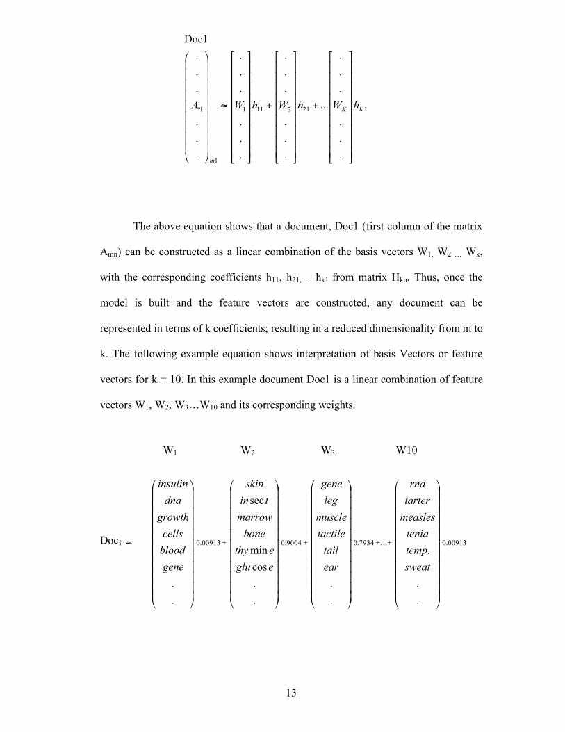
The above equation shows that a document, Doc1 (first column of the matrix

Amn) can be constructed as a linear combination of the basis vectors W1, W2 … Wk,

with the corresponding coefficients h11, h21, … hk1 from matrix Hkn. Thus, once the

model is built and the feature vectors are constructed, any document can be

represented in terms of k coefficients; resulting in a reduced dimensionality from m to

k. The following example equation shows interpretation of basis Vectors or feature

vectors for k = 10. In this example document Doc1 is a linear combination of feature

vectors W1, W2, W3…W10 and its corresponding weights.

Doc1 !

!!!!!!!!!!!

"

#

$$$$$$$$$$$

%

&

.

.

gene

blood

cells

growth

dna

insulin

0.00913 +

!!!!!!!!!!!

"

#

$$$$$$$$$$$

%

&

.

.

cos

min

sec

eglu

ethy

bone

marrow

tin

skin

0.9004 +

!!!!!!!!!!!

"

#

$$$$$$$$$$$

%

&

.

.

ear

tail

tactile

muscle

leg

gene

0.7934 +…+

!!!!!!!!!!!

"

#

$$$$$$$$$$$

%

&

.

.

.

sweat

temp

tenia

measles

tarter

rna

0.00913

1212111

1

1*

.

.

.

.

.

.

...

.

.

.

.

.

.

.

.

.

.

.

.

.

.

.

.

.

.

KK

m

hWhWhWA

!!!!!!!!!

"

#

$$$$$$$$$

%

&

+

!!!!!!!!!

"

#

$$$$$$$$$

%

&

+

!!!!!!!!!

"

#

$$$$$$$$$

%

&

'

(((((((((

)

*

+++++++++

,

-

Doc1

W1 W2 W3 W10

14

The NMF decomposition is non-unique; the matrices W and H depend on the

NMF algorithm employed and the error measure used to check convergence. Some of

the NMF algorithm types are, multiplicative update algorithm by Lee and Seung [9],

gradient descent algorithm by Hoyer [34] and alternating least squares algorithm by

Pattero [35]. In the Oracle database tools employed in this work, the multiplicative

update algorithm was used for NMF feature extraction.

The NMF algorithm iteratively updates the factorization based on a given

objective function [33]. The general objective function is to minimize the Euclidean

distance between each column of the matrix Amn and its approximation Amn ≈ Wmk ×

Hkn. Using the Frobenius norm for matrices, the objective function is,

Lee and Seung [9] employed the following multiplicative update rules to achieve

convergence.

In other words, the (t+1)th approximation is obtained from tth approximation as shown

below.

( ) ∑ ∑ ∑ ∑ = = = =

− ≡ − = − ≡ Θ n

j

m

i

n

j

k

l lj il ij F j j E H W A WH A Wh a H W

1 1 1

2

1 2 2

2 ,

[ ] [ ]

aj T

aj T

aj aj WH W A W

H H ←

[ ] [ ]

ja T

ja T

ia ia WHH AH

W W ←

aj t T t

E t

aj t

aj H A W Q H H ) , , ( ) ( ) ( ) ( ) 1 ( = +

ia t t T

E t

ia t

ia W H A Q W W ) , , ( ) ( ) 1 ( ) ( ) 1 ( + + =

15

Lee and Seung [9] proved that the above update rules achieve monotonic

convergence. Clearly, the accuracy of the approximation depends on the value of k,

which is the number of feature vectors. In the current work, k is user defined. A

systematic study has been carried out to investigate the influence of k on the accuracy

of the model, when combined with the support vector machine algorithm (SVM) for

text classification.

2.6 Similarity and Term weight of text documents

When we deal with text documents we have to consider two important aspects: Term

weight and Similarity measure.

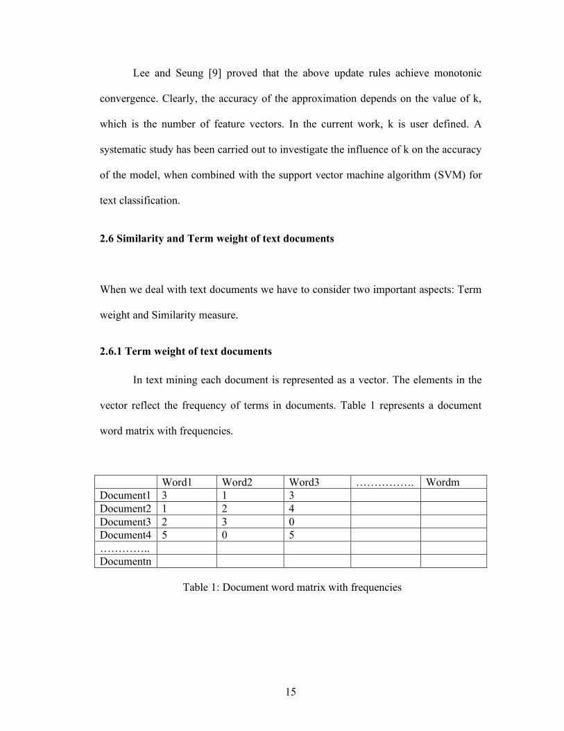
2.6.1 Term weight of text documents In text mining each document is represented as a vector. The elements in the

vector reflect the frequency of terms in documents. Table 1 represents a document

word matrix with frequencies.

Word1 Word2 Word3 ……………. Wordm Document1 3 1 3 Document2 1 2 4 Document3 2 3 0 Document4 5 0 5 ………….. Documentn Table 1: Document word matrix with frequencies

16

In Table 1, the numbers in each row represent the term frequencies, tf, of the

keywords in documents 1, 2, 3… n.

Figure 1: Three-dimensional term space

In text mining each word is a dimension and documents are vectors as shown

in Figure 1. Each word in a document has weights. These weights can be of two

types: Local and global weights. If local weights are used, then term weights are

normally expressed as term frequencies, tf. If global weights are used, Inverse

Document Frequency, IDF values, gives the weight of a term.

Document 4 (5, 0, 5)

(0,1,0) Word1

Document3 (2, 3, 0)

(1,0,0) Word2 Document1 (3,1,3)

(0, 0, 1) Word3 θ

17

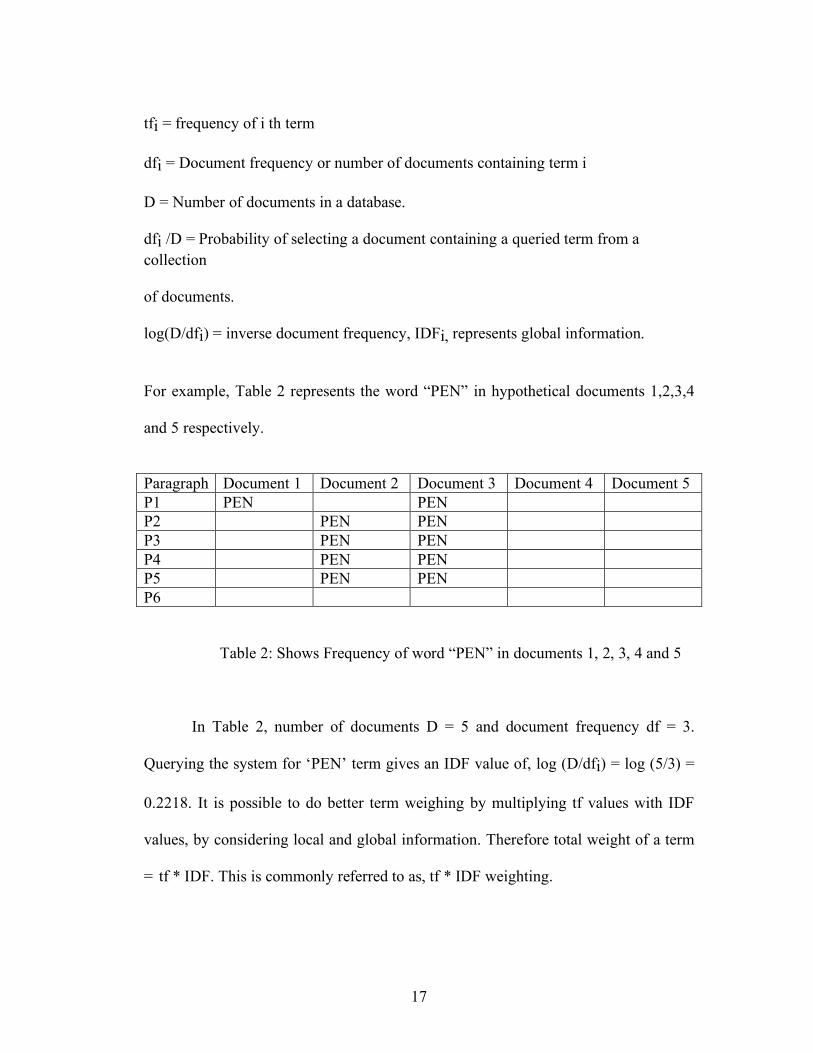
tfi = frequency of i th term dfi = Document frequency or number of documents containing term i D = Number of documents in a database. dfi /D = Probability of selecting a document containing a queried term from a collection of documents. log(D/dfi) = inverse document frequency, IDFi, represents global information.

For example, Table 2 represents the word “PEN” in hypothetical documents 1,2,3,4

and 5 respectively.

Paragraph Document 1 Document 2 Document 3 Document 4 Document 5 P1 PEN PEN P2 PEN PEN P3 PEN PEN P4 PEN PEN P5 PEN PEN P6 Table 2: Shows Frequency of word “PEN” in documents 1, 2, 3, 4 and 5

In Table 2, number of documents D = 5 and document frequency df = 3.

Querying the system for ‘PEN’ term gives an IDF value of, log (D/dfi) = log (5/3) =

0.2218. It is possible to do better term weighing by multiplying tf values with IDF

values, by considering local and global information. Therefore total weight of a term

= tf * IDF. This is commonly referred to as, tf * IDF weighting.

18

2.6.2 Similarity measure of documents

If two documents describe similar topics, employing nearly the same

keywords, these texts are similar and their similarity measure should be high. Usually

dot product represents similarity of the documents. To normalize the dot product we

divide it by the Euclidean distances of the two documents represented respectively by

Doc1 and Doc2; i.e., <Doc1, Doc2> / (|Doc1||Doc2|). Here |Doc1|, |Doc2| represent

magnitudes of vectors Doc1 and Doc2 respectively and <Doc1, Doc2> is the dot

product of the vectors Doc1 and Doc2. This ratio defines the cosine angle between

the vectors, with values between 0 and 1 [25]. This is called cosine similarity.

Figure 2: Straight lines in 2-Dimensional space represent Euclidean distances of

document vectors Doc1 and Doc2, with origin O.

Y-axis (word or category)

Doc1

Doc2

X-axis (word or category) O

θ

19

Similarity of the vectors Doc1 and Doc2 = cos θ = <Doc1, Doc2> / |Doc1||Doc2| As the angle between the vectors, θ, decreases, the cosine angle approaches to 1,

meaning that the two document vectors are getting closer, and the similarity of the

vectors increases.

20

CHAPTER 3

METHODOLOGY

The following sections describe some details of support vector machine (SVM)

algorithm and multi class and multi target problems. In this thesis SVM is used for

classification of text data. If a training data is linearly separable then the simplest

classifier that can be used for classification is a linear classifier. The following section

describes about linear classifiers.

3.1 Linear classifiers

Linear classifiers define a hyper plane in the input space. The hyper plane

given by the equation, <X, W> + b = 0 defines a (d - 1) dimensional hyper plane in

the vector space Rd, which is the decision boundary of the discriminant function,

where <X, W> is dot product of the vectors X and W. The vector W is a normal

vector for this hyper plane, which for b = 0 passes through the origin and the vector X

is a data point in the vector space Rd. In the Figure 3, X can be either a circle or a

square. For linear classifiers we want to find W and b such that <W, X> + b > 0 for

circles <W, X> + b < 0 for squares as shown in Fig. 4 [3].

21

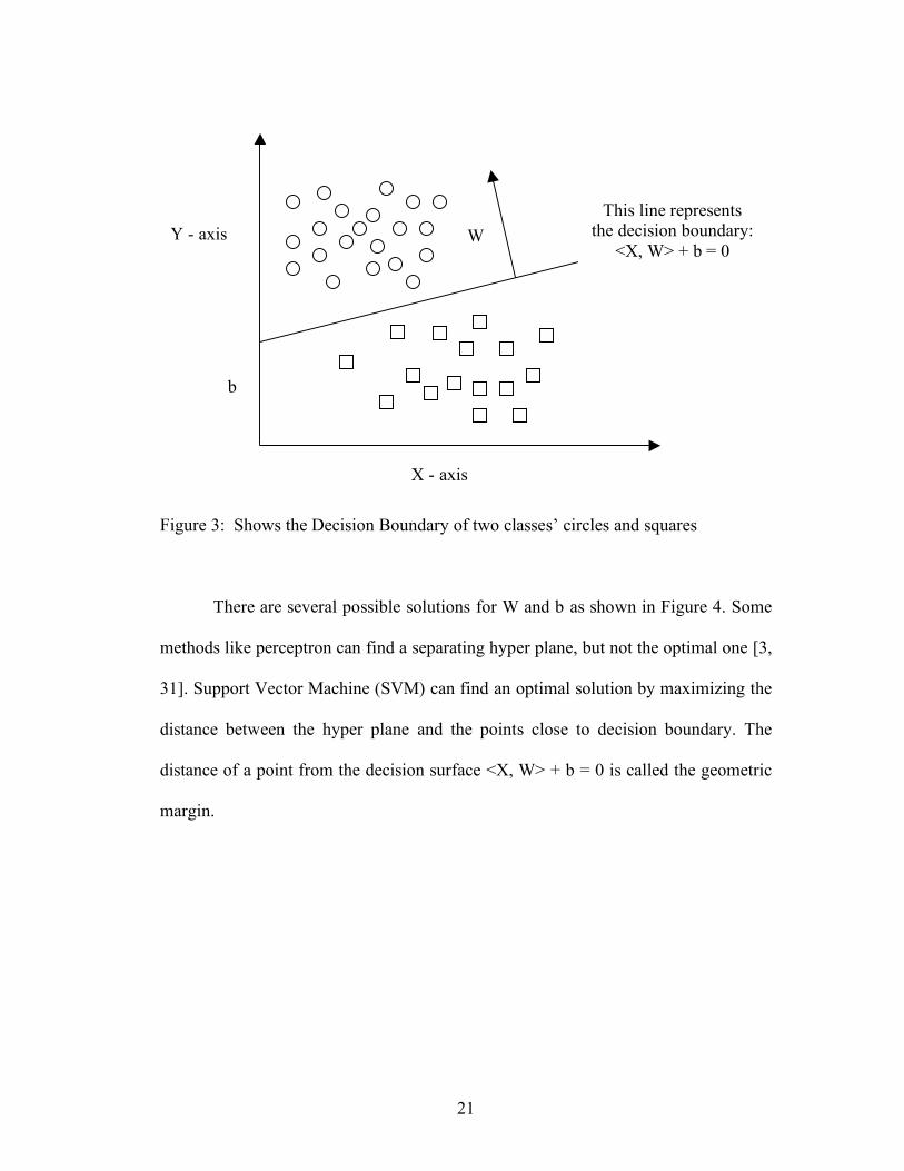
Figure 3: Shows the Decision Boundary of two classes’ circles and squares

There are several possible solutions for W and b as shown in Figure 4. Some

methods like perceptron can find a separating hyper plane, but not the optimal one [3,

31]. Support Vector Machine (SVM) can find an optimal solution by maximizing the

distance between the hyper plane and the points close to decision boundary. The

distance of a point from the decision surface <X, W> + b = 0 is called the geometric

margin.

This line represents the decision boundary:

<X, W> + b = 0

X - axis

Y - axis W

b

22

Figure 4: Shows possible decision boundaries.

Figure 5: Shows the Margin.

All these lines can represent the decision

boundary

X - axis

Y - axis

Our goal is to maximize the margin as much as we can.

X - axis

Y - axis

23

The distance between two supporting hyper planes is called margin as shown

in Fig. 6. The main goal here is to maximize the margin so that the classifier can

separate classes clearly. Maximizing the margin is a Quadratic programming problem

[3, 11].

3.2 Support vectors

A Support Vector Machine (SVM) is a learning machine that classifies an

input vector X using the decision function: f (X) = <X, W>+ b. SVMs are hyper plane

classifiers and work by determining which side of the hyper plane X lies. In the above

formula, the hyper plane is perpendicular to W and at a distance b / ||W|| from the

origin. SVM maximize the margin around the separating hyper plane. The decision

function is fully specified by a subset of training samples. This subset of vectors is

called the support vectors [16].

24

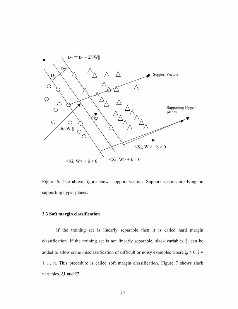
Figure 6: The above figure shows support vectors. Support vectors are lying on

supporting hyper planes.

3.3 Soft margin classification

If the training set is linearly separable then it is called hard margin

classification. If the training set is not linearly separable, slack variables ξi can be

added to allow some misclassification of difficult or noisy examples where ξi > 0, i =

1 … n. This procedure is called soft margin classification. Figure 7 shows slack

variables, ξ1 and ξ2.

Supporting Hyper planes

D+ D-

D+ + D- = 2/||W||

W

-b/||W ||

<Xi, W> + b < 0

<Xi, W >+ b > 0

<Xi, W> + b = 0

Support Vectors

25

Figure 7: Shows Noisy examples.

Noisy or Difficult examples

X - axis

Y - axis

ξ1

ξ2

26

3.4 Non-linear classifiers

The slack variable approach is not a very efficient technique for classifying

non-separable classes in input space. In Figure 8, the classes are separated by a

polynomial shaped surface (a non-linear classifier) in the input space, rather than a

hyper plane. In this case soft margin classification is not applicable because the data

is not linearly separable.

Figure 8: Shows non-linear classifier.

X - Axis

Y - Axis

27

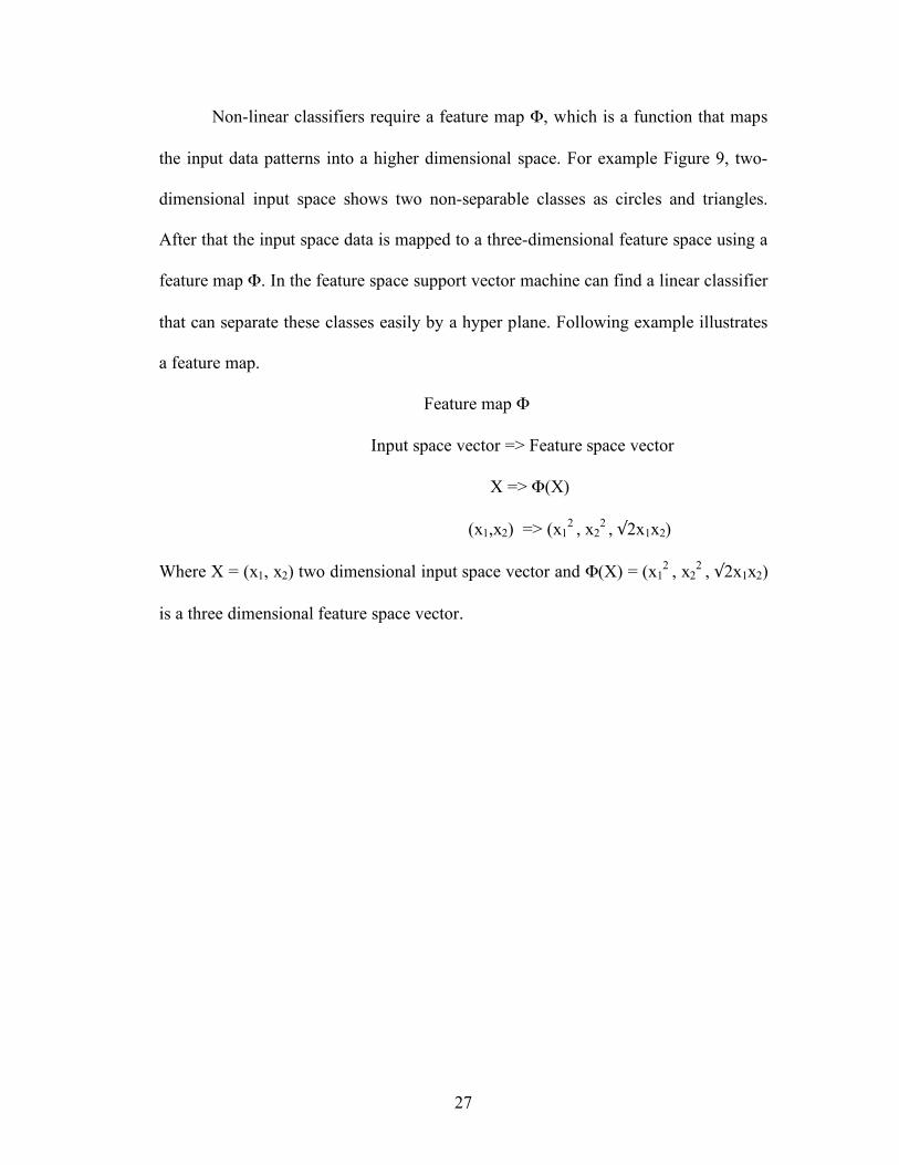
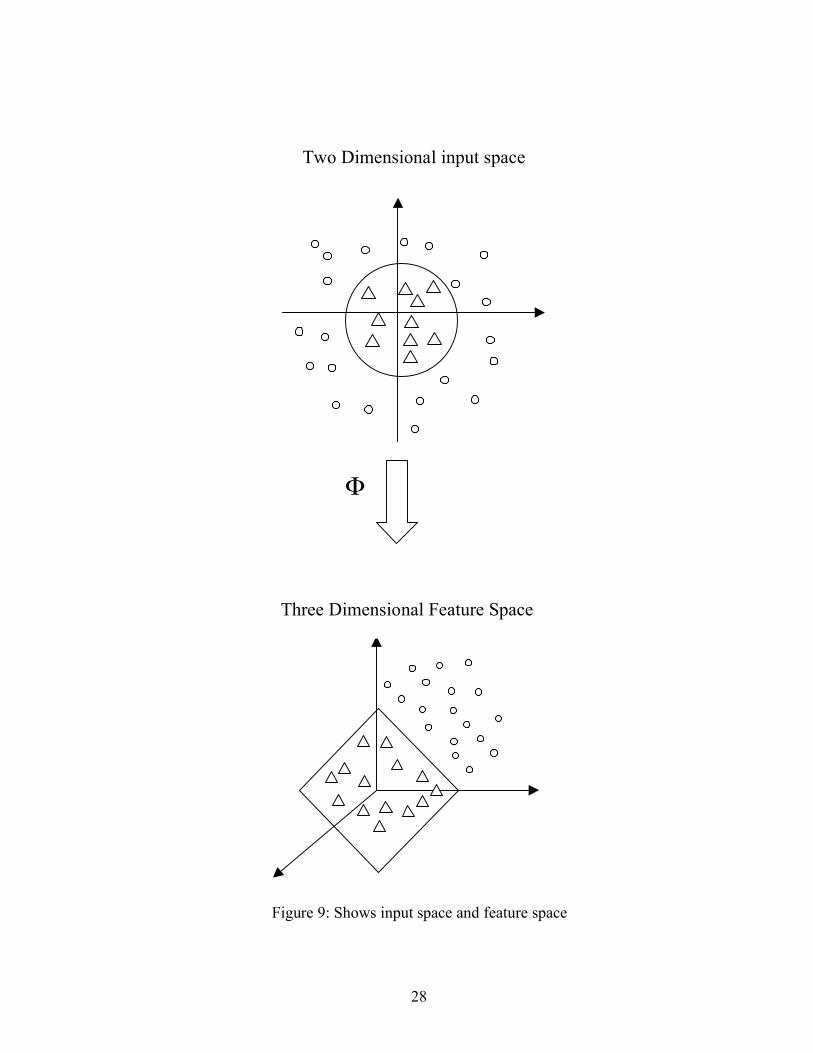
Non-linear classifiers require a feature map Φ, which is a function that maps

the input data patterns into a higher dimensional space. For example Figure 9, two-

dimensional input space shows two non-separable classes as circles and triangles.

After that the input space data is mapped to a three-dimensional feature space using a

feature map Φ. In the feature space support vector machine can find a linear classifier

that can separate these classes easily by a hyper plane. Following example illustrates

a feature map.

Feature map Φ

Input space vector => Feature space vector

X => Φ(X)

(x1,x2) => (x12

, x22 , √2x1x2)

Where X = (x1, x2) two dimensional input space vector and Φ(X) = (x12

, x22 , √2x1x2)

is a three dimensional feature space vector.

28

Figure 9: Shows input space and feature space

Three Dimensional Feature Space

Two Dimensional input space

Φ

29

The number of features of degree g over an input space dimension d will be

given by . For a data of 100-dimensional, all second order features are

5000. The feature map approach inflates the input representation. It is not scalable,

unless small subset of features is used. The explicit computation of the feature map Φ

can be avoided, if the learning algorithm would just depend on inner products, SVM

decision function is always in terms of dot products.

Kernel functions

Kernels functions are used for mapping the input space to a feature space

instead of a feature mapΦ, if the operations on classes are always dot products. In this

way complexity of calculating Φ can be reduced [22]. The main optimization

function of SVM can be re-written in the dual form where data appears only as inner

product between data points. Kernel, K is a function that returns the inner product of

two data points,

K(X1, X2) = <Φ(X1), Φ(X2)>

Let’s consider two dimensional input space vectors x = (x1,x2), z = (z1,z2), and the

simple polynomial kernel function k (x, z) = 〈x,z〉2 . We can represent this kernel

function into <Φ(x), Φ(z)> as follows:

〈x,z〉2 =(x1 z1 + x2 z2)2 = x12 z1

2 + x2

2 z22 + 2x1 z1x2 z2

= 〈(x12

, x22 , √2x1x2),(z1

2 , z22 , √2z1z2)〉

=〈φ(x), φ(z)〉

Therefore, kernel function can be calculated without calculating φ(x) such as

30

〈x,z〉2 =(x1 z1 + x2 z2)2. Here the feature map Φ is never explicitly computed. Hence,

kernels avoid the task of actual mapping of Φ(X). This is called kernel trick [22].

Computing kernel, K is equivalent to mapping data patterns into a higher dimensional

space and then taking the dot product there. Using this kernel approach, support

vector machine exploit information about the inner product between data points into

feature space. Kernels map data points into feature space where they are more easily

possibly linearly separable. In order to classify non-separable classes kernel technique

is a best approach. SVM performs a nonlinear mapping of the input vector from the

input space into a higher dimensional Hilbert space, where the mapping is determined

by the kernel function. Two typical kernel functions are listed below:

K(X1, X2) = (<X1, X2> + C) d, where C >= 0 --- Polynomial Kernel

Where d is the dimension and C is a constant. X1 and X2 are input space vectors.

K(X1, X2) = exp(- (||X1 – X2 || 2) / 2(σ 2)) --- Gaussian Kernel

Where ‘σ’ is the bandwidth of a gaussian curve. Here the term ||X1 – X2|| represents

distance between the vectors X1 and X2.

31

3.5 Multi-class and Multi-target problems

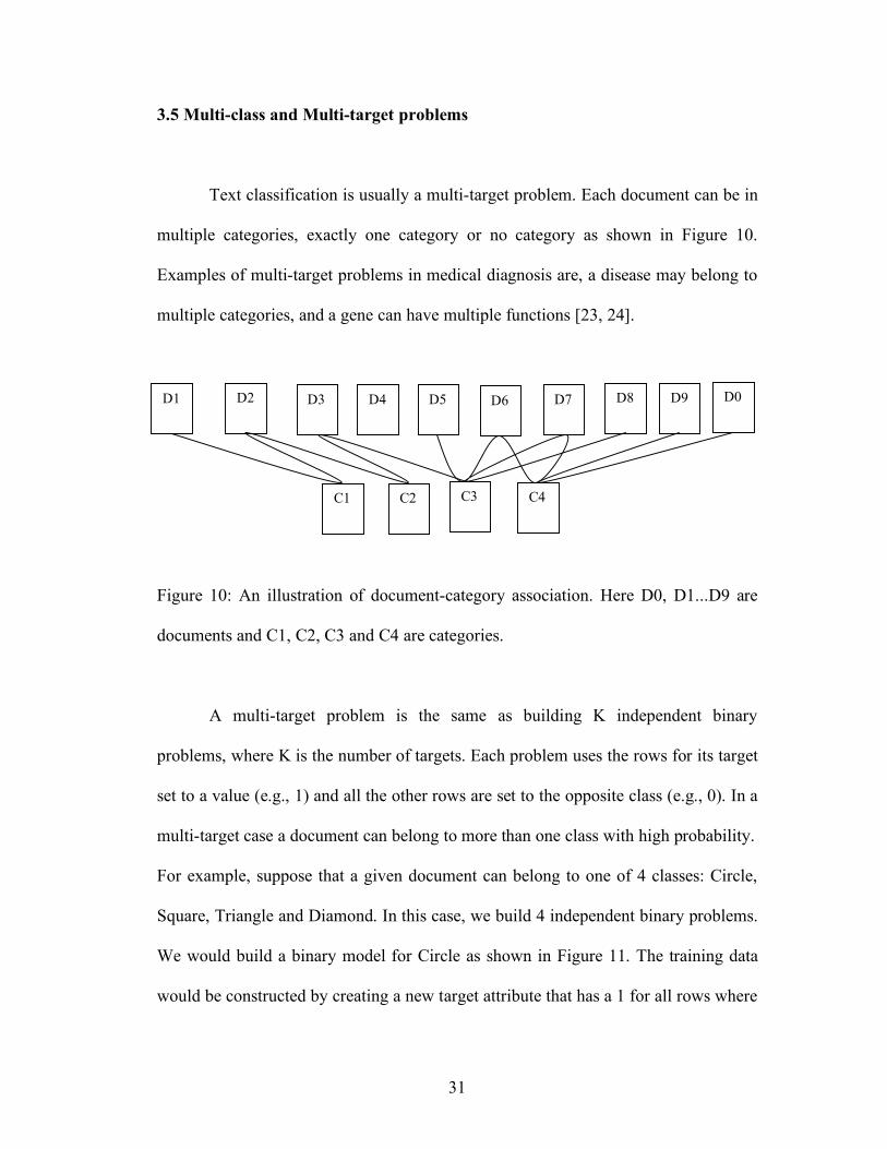
Text classification is usually a multi-target problem. Each document can be in

multiple categories, exactly one category or no category as shown in Figure 10.

Examples of multi-target problems in medical diagnosis are, a disease may belong to

multiple categories, and a gene can have multiple functions [23, 24].

Figure 10: An illustration of document-category association. Here D0, D1...D9 are

documents and C1, C2, C3 and C4 are categories.

A multi-target problem is the same as building K independent binary

problems, where K is the number of targets. Each problem uses the rows for its target

set to a value (e.g., 1) and all the other rows are set to the opposite class (e.g., 0). In a

multi-target case a document can belong to more than one class with high probability.

For example, suppose that a given document can belong to one of 4 classes: Circle,

Square, Triangle and Diamond. In this case, we build 4 independent binary problems.

We would build a binary model for Circle as shown in Figure 11. The training data

would be constructed by creating a new target attribute that has a 1 for all rows where

D1 D2 D3 D4 D5 D6 D7 D8 D9

C2 C1 C3 C4

D0

32

class is Circle and 0 otherwise. This would be repeated to create a binary model for

each class. In this case, after a model is built, when a new document arrives, the SVM

uses its 4 binary models and determines that the document belongs to one or more of

the 4 classes. A document, in a multi-target problem, belongs to more than one class.

If a document belongs only to a single class, it would be a multi-class problem. Each

binary problem is built using all the data.

Figure 11: Multi-class classification.

X - axis

Y - axis

This line represents a Binary Classifier of circles and rest of the symbols

33

CHAPTER 4

IMPLEMENTATION

A text classification problem consists of training examples, testing examples

and new examples. Each training example has one target attribute and multiple

predictor attributes. Testing examples are used to evaluate the models; hence they

have both predictor and target attributes. New examples consist of predictor

attributes only. The goal of text classification is to construct a model as a function of

the values of the attributes using training examples/documents, which would then

predict the target values of the new examples/documents as accurately as possible.

Thus, in building a classification model, the first task is to train the

classification algorithm with a set of training examples. During training, the

algorithm finds relationships between the predictor attribute values and the target

attribute values. These relationships are summarized in a model, which can be applied

to new examples to predict their target values. After constructing the model, the next

task is to test it. The constructed classification model is used to evaluate data with

known target values (i.e. data with testing examples) and compare them with the

model predictions. This procedure calculates the model’s predictive accuracy. After

refining the model to achieve satisfactory accuracy, it will be used to score new data,

i.e. to classify new examples according to the user defined criteria.

The first step in text mining is text gathering. The process of text gathering in

MEDLINE database is usually done by Pub Med [29]. The Pub Med database

34

contains 12,000,000 references of biomedical publications. MEDLINE database is a

subset of Pub Med. A subset of the MEDLINE database was used for this thesis. The

second step is text preprocessing.

Preprocessing steps for text mining

Text preprocessing involves extracting the actual text context, loading text

data to database, document indexing and feature extraction.

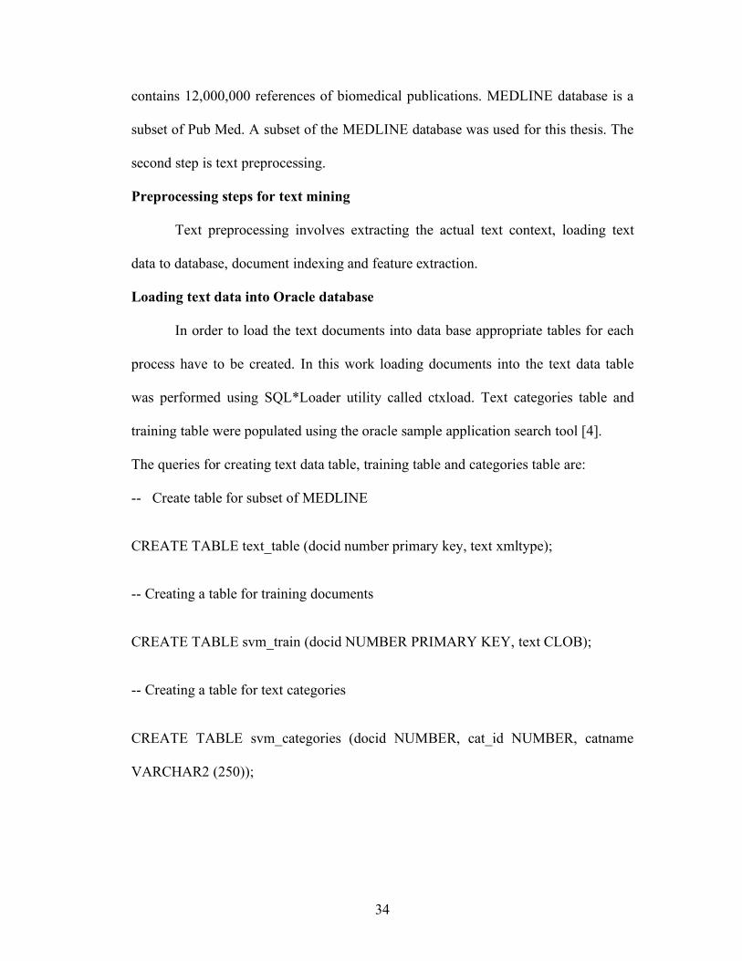
Loading text data into Oracle database

In order to load the text documents into data base appropriate tables for each

process have to be created. In this work loading documents into the text data table

was performed using SQL*Loader utility called ctxload. Text categories table and

training table were populated using the oracle sample application search tool [4].

The queries for creating text data table, training table and categories table are:

-- Create table for subset of MEDLINE

CREATE TABLE text_table (docid number primary key, text xmltype);

-- Creating a table for training documents

CREATE TABLE svm_train (docid NUMBER PRIMARY KEY, text CLOB);

-- Creating a table for text categories

CREATE TABLE svm_categories (docid NUMBER, cat_id NUMBER, catname

VARCHAR2 (250));

35

Querying for text data to construct text categories table or training table:

This section shows some example queries for retrieving the text documents

of a specified category using CONTAINS, ABOUT, $ query operators in oracle text

mining:

-- Using CONTAINS operator for key word search

SELECT text FROM text_table WHERE CONTAINS (text, 'Cell') > 0;

-- Using ABOUT operator to narrow things down:

SELECT text FROM text_table WHERE CONTAINS (text, ‘about (Gene)', 1) > 0;

-- Using $ for Stem searching

SELECT text FROM text_table WHERE CONTAINS (text, '$Blood', 1) > 0;

Indexing text documents:

Document Indexing means preparing the raw document collection into an

easily accessible representation of documents. This is normally done using following

steps: tokenization, filtration, stemming, and weighting.

Tokenization means text is parsed, lowercased and all punctuations are removed.

Filtration refers to the process of deciding which terms should be used to represent

the documents so that these can be used for describing the document's content,

discriminating the document from the other documents in the collection, and

frequently used terms or stop words (is, of, in …) are removed from term streams.

Stemming refers to the process of reducing terms to their stems or root variant. Thus,

"computer", "computing", "compute" is reduced to "comput".

Weighting means terms are weighted according to a given weighting model.

36

Query for building an index on a database column containing text:

CREATE INDEX texttab_idx ON text_table (text) INDEXTYPE IS

CTXSYS.CONTEXT

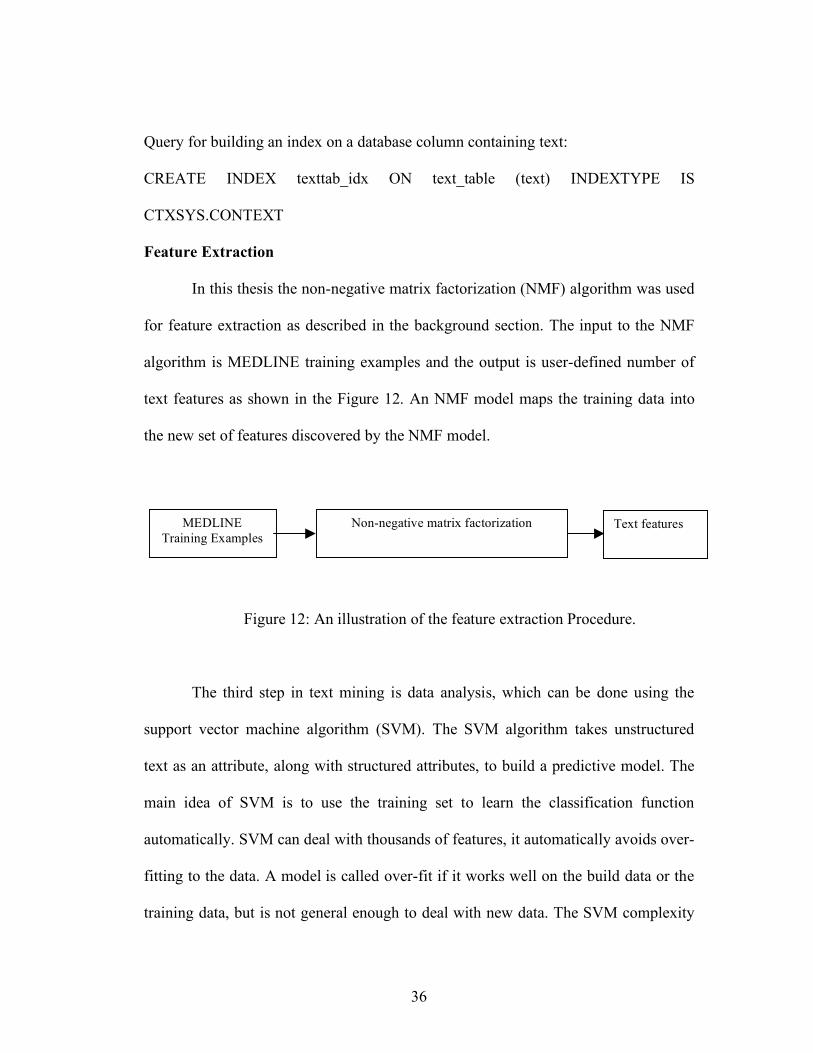
Feature Extraction

In this thesis the non-negative matrix factorization (NMF) algorithm was used

for feature extraction as described in the background section. The input to the NMF

algorithm is MEDLINE training examples and the output is user-defined number of

text features as shown in the Figure 12. An NMF model maps the training data into

the new set of features discovered by the NMF model.

Figure 12: An illustration of the feature extraction Procedure.

The third step in text mining is data analysis, which can be done using the

support vector machine algorithm (SVM). The SVM algorithm takes unstructured

text as an attribute, along with structured attributes, to build a predictive model. The

main idea of SVM is to use the training set to learn the classification function

automatically. SVM can deal with thousands of features, it automatically avoids over-

fitting to the data. A model is called over-fit if it works well on the build data or the

training data, but is not general enough to deal with new data. The SVM complexity

Non-negative matrix factorization Text features MEDLINE Training Examples

37

factor prevents over fitting by finding the best tradeoff between simplicity and

complexity and maximizes predictive accuracy [3]. Figure 13 is a schematic

illustration of model complexity and error. The graph shows two curves, training set

curve and testing set curve. If the model is too simple, model error is high and it

under fits the data. If the model is too complex, the error goes down but it over fits

the data, resulting in an increased error when applied on the test data. The figure

illustrates that there is an ideal level of complexity, which minimizes the prediction

error when applied to the test set or new data.

Figure 13: The above figure shows the graph of model error and model complexity.

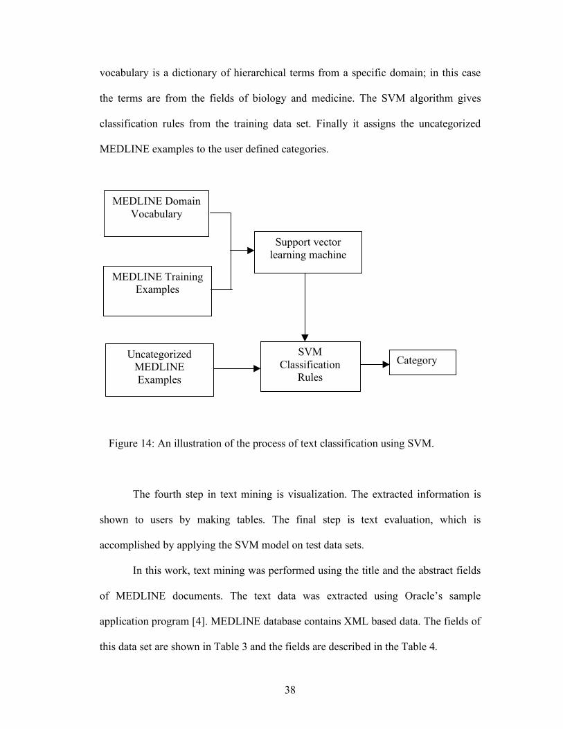
As shown in the Figure 14, the support vector machines algorithm takes the

MEDLINE training examples and the domain vocabulary as the input. Here domain

Model Complexity

Error

Training Set

Testing set

Model over fitting Model Under fitting

Ideal model

38

vocabulary is a dictionary of hierarchical terms from a specific domain; in this case

the terms are from the fields of biology and medicine. The SVM algorithm gives

classification rules from the training data set. Finally it assigns the uncategorized

MEDLINE examples to the user defined categories.

Figure 14: An illustration of the process of text classification using SVM.

The fourth step in text mining is visualization. The extracted information is

shown to users by making tables. The final step is text evaluation, which is

accomplished by applying the SVM model on test data sets.

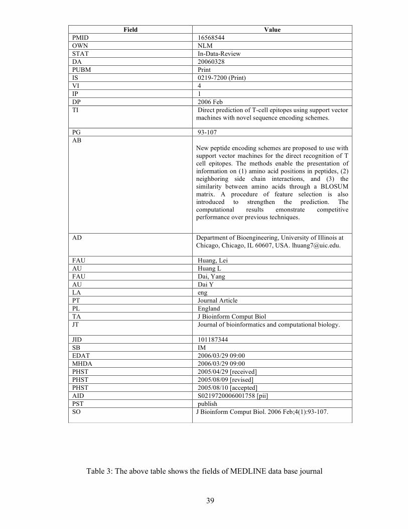
In this work, text mining was performed using the title and the abstract fields

of MEDLINE documents. The text data was extracted using Oracle’s sample

application program [4]. MEDLINE database contains XML based data. The fields of

this data set are shown in Table 3 and the fields are described in the Table 4.

SVM Classification

Rules

MEDLINE Training Examples

Uncategorized MEDLINE Examples

Support vector learning machine

Category

MEDLINE Domain Vocabulary

39

Table 3: The above table shows the fields of MEDLINE data base journal

Field Value PMID 16568544 OWN NLM STAT In-Data-Review DA 20060328 PUBM Print IS 0219-7200 (Print) VI 4 IP 1 DP 2006 Feb TI Direct prediction of T-cell epitopes using support vector

machines with novel sequence encoding schemes.

PG 93-107 AB

New peptide encoding schemes are proposed to use with support vector machines for the direct recognition of T cell epitopes. The methods enable the presentation of information on (1) amino acid positions in peptides, (2) neighboring side chain interactions, and (3) the similarity between amino acids through a BLOSUM matrix. A procedure of feature selection is also introduced to strengthen the prediction. The computational results emonstrate competitive performance over previous techniques.

AD Department of Bioengineering, University of Illinois at Chicago, Chicago, IL 60607, USA. [email protected].

FAU Huang, Lei AU Huang L FAU Dai, Yang AU Dai Y LA eng PT Journal Article PL England TA J Bioinform Comput Biol JT Journal of bioinformatics and computational biology.

JID 101187344 SB IM EDAT 2006/03/29 09:00 MHDA 2006/03/29 09:00 PHST 2005/04/29 [received] PHST 2005/08/09 [revised] PHST 2005/08/10 [accepted] AID S0219720006001758 [pii] PST publish SO J Bioinform Comput Biol. 2006 Feb;4(1):93-107.

40

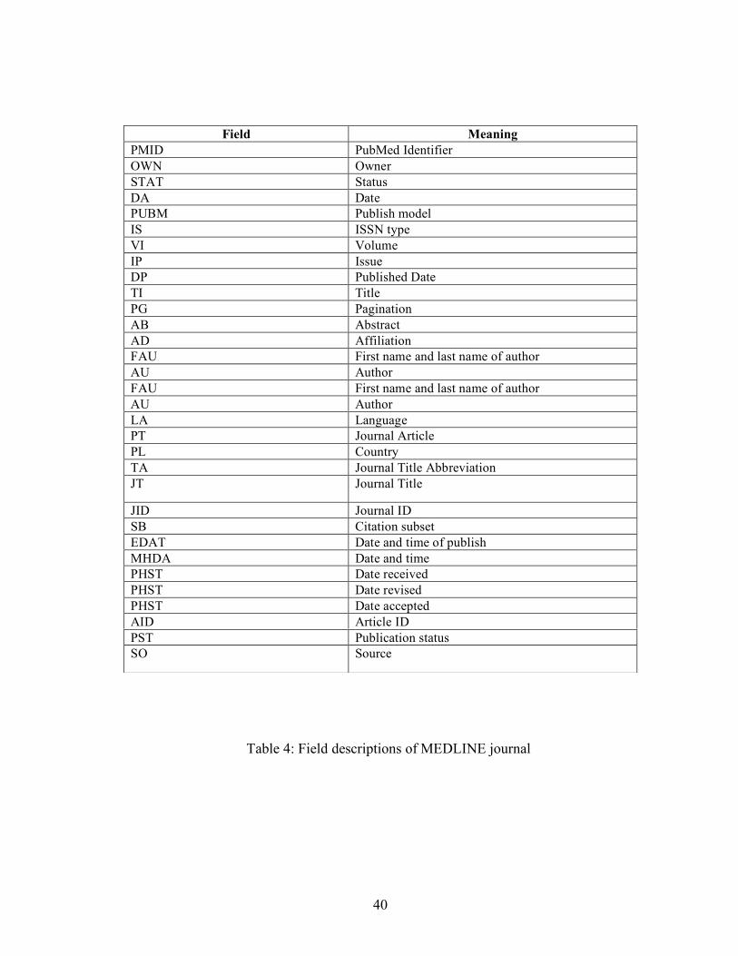
Table 4: Field descriptions of MEDLINE journal

Field Meaning PMID PubMed Identifier OWN Owner STAT Status DA Date PUBM Publish model IS ISSN type VI Volume IP Issue DP Published Date TI Title PG Pagination AB Abstract AD Affiliation FAU First name and last name of author AU Author FAU First name and last name of author AU Author LA Language PT Journal Article PL Country TA Journal Title Abbreviation JT Journal Title

JID Journal ID SB Citation subset EDAT Date and time of publish MHDA Date and time PHST Date received PHST Date revised PHST Date accepted AID Article ID PST Publication status SO Source

41

4.1 SVM algorithm parameter description

SVM algorithm takes several parameters such as convergence tolerance value,

complexity factor, cache size, and standard deviation [13]. The following sections

describe these parameters in more detail. The values used for these parameters in the

current investigation are displayed in the result section.

4.1.1 Convergence tolerance value

Convergence tolerance value is the maximum size of a violation of the

convergence criterion such that the model is considered to have converged. The

tolerance value is the error that a user can specify so that the model is considered to

be converged, i.e. a hyper plane has been found which classifies the training data set

within the specified error limit. Larger values of the tolerance result in faster model

building, but the resulting models are less accurate. Decreasing the tolerance value

leads to a more accurate classification model; however it takes longer time for the

computed hyper plane to converge.

4.1.2 Complexity factor

The complexity factor is also known as capacity or penalty. It determines the

trade-off between minimizing model error on the training data and minimizing model

complexity. Its responsibility is to avoid over-fitting or under-fitting of the model. An

over-complex model fits the noise in the training data and an over simple model

42

under-fits the training data. A very large value of the complexity factor leads to an

extreme penalty on errors; in this case SVM seeks a perfect separation of target

classes. A small value for the complexity factor places a low penalty on errors and

high constraints on the model parameters, which can lead to an under-fit.

4.1.3 Kernel cache size

Using the gaussian kernel require the specification of the size of the cache

used for storing computed kernels during the training operation. Computation of

kernels in a gaussian SVM model is a very expensive operation. SVM model

converges within a chunk of data at a time, and then it tests for violators outside of

the chunk. Training is complete when there are no more violators within the

tolerance. Generally, larger caches lead to faster model building [13, 18].

4.1.4 Standard deviation

Standard deviation is a measure of the distance between the target classes.

Standard deviation is a kernel parameter for controlling the spread of the gaussian

function and thus the smoothness of the SVM solution. Distances between records

grow with increasing dimensionality, in which case the standard deviation needs to be

scaled accordingly.

43

Optimal parameter search procedure:

Building NMF and SVM models requires optimizing certain parameters to

arrive at the best accuracy. The following procedure was followed in determining the

optimal parameters. Suppose that the number of parameters to be optimized is n. The

default values of the Oracle software were taken as the initial values. Then, parameter

1 is perturbed, while keeping the remaining (n-1) parameters constant. When the

optimal value is found for the first parameter, the procedure is then repeated for the

remaining parameters, while keeping the others constant. After the optimal value for

parameter n is found, parameter 1 is again perturbed to determine if it still has the

optimal value. If its optimal value changed, the new value is then determined. The

procedure is then repeated iteratively until all parameters are optimal and the best

accuracy is achieved. In most of the cases in the current work, one iteration was

sufficient to arrive at the optimal values.

44

CHAPTER 5

EXPERIMENTS AND RESULTS

In this work, multi-class classification with a subset of MEDLINE data was

performed using the support vector machine (SVM) and the non-negative matrix

factorization (NMF) algorithms in the Oracle data mining software. This section

describes the data sets and tables used in the experiments on MEDLINE data and the

results.

5.1 Dataset description

A subset of the MEDLINE data was used for the experiments. The total data

set was divided into two subsets. One subset is used for training the algorithm and the

other subset is used for testing the algorithm. Eighty percent of the total data is used

for training and the remaining twenty percent of the data is used for testing. Some

details of the data set are given below.

Total MEDLINE documents: 300 Approximate number of words in each document: 350 Training documents: 240 Testing documents: 60

45

DOCID Text

15,143,089 Characterization of intercellular adhesion molecule-1 and HLA-DR…..

15,140,540 Expression profile of an androgen regulated prostate specific homeobox ..

15,139,712 Suramin suppresses hypercalcemia and osteoclastic bone resorption…..

15,138,573 The anchoring filament protein kalinin is synthesized and secreted…..

15,138,566 Outcome from mechanical ventilation after autologous peripheral…..

15,138,488 Effects of synthetic peptido-leukotrienes on bone resorption in vitro…..

15,134,383 Functional role of sialyl Lewis X and fibronectin-derived RGDS peptide..

15,133,039 Thyroid cancer after exposure to external radiation: a pooled analysis of

Table 5: A sample text data table

Table 5 shows a typical text data table used in the experiments. The table

contains the text and the document identifier for each document. A table of text

categories is then constructed, a small portion of which is shown in Table 6, which

shows the category names (e.g. cell, gene, and blood), the corresponding category

identification number (ID) and the text documents. Each category can have any

number of documents. In the classification model, the target attribute is the category

name. Table 5 and Table 6 are not showing all the text of title and abstract fields.

Table 3 shows full text of title of abstract fields of a text document.

46

DOCID Category ID Category

name Text

12,415,630 1 CELL P-glycoprotein expression

by cancer cells affects

8,868,467 1 CELL CD44/chondroitin sulfate proteoglycan and alp

11,001,907 1 CELL Syndecan-1 is targeted to the uropods of polarize

12,846,806 2 GENE Cell-cycle control of plasma cell differentiation

7,682,288 2 GENE Altered metabolism of mast-cell growth factor

8,604,398 2 GENE Differentiation pathways and histogenetic

11,272,902 3 BLOOD Detection of clonally restricted immunoglobulin

11,286,632 3 BLOOD PTCH mutations in squamous cell carcinoma of

10,792,179 3 BLOOD Phenotypic and genotypic characterization

Table 6: Table of text categories for the support vector machine algorithm.

5.2 Results of Text mining with SVM Alone

Since text-mining models based on SVM alone use documents with full

dimensionality (i.e. all distinct keywords in the text documents), their classification

performance is very good; however, they are computationally expensive. On the test

data set, the dimensionality is several thousands and the SVM models achieved a

maximum accuracy of approximately 98%. A summary of the results from using the

47

SVM alone is shown below. They represent the most accurate results from all the

experiments in which the model parameters were varied.

Oracle data mining results with SVM alone, using a Linear Kernel Model settings: Convergence tolerance value = 0.001

Complexity factor = 0.2

Accuracy: 98% Oracle data mining results with SVM alone using a Gaussian Kernel Model settings: Convergence tolerance value = 0.001

Kernel cache size = 50000000 bytes

Complexity factor = 20

Standard deviation = 6.578

Accuracy: 81%

From the above experiments with Linear and gaussian kernels in the Oracle

data mining (ODM) SVM tool, it was found that the linear kernel performs better

than Gaussian kernel for text mining with MEDLINE database. Usually if the number

of attributes is more than 1000, the gaussian kernel is thought to give the best results.

However, in the above experiments the linear kernel was found to perform better. In

order to understand this difference, a literature search was conducted. It was found

48

that a few other studies have been done on support vector machines by comparing

them with other supervised learning techniques such as decision tree classifier and the

Naïve Bayesian. Linear, polynomial, and gaussian kernels have all been tested on

different classification algorithms. It was reported that the linear SVMs perform as

well as the more complicated kernel based SVMs if they have high enough input

space. This implies that, the text categories are linearly separable in the feature space.

Whenever they are linearly separable, linear kernels perform as good as the more

complex kernels.

5.3 Results of Text mining with NMF and SVM

Feature extraction through the non-negative matrix factorization (NMF)

algorithm is used to reduce the dimensionality of the text documents. This was

accomplished in the Oracle data mining software, which has the NMF algorithm, built

in it. Following the feature extraction to reduce the dimensionality, the SVM

algorithm was used to classify the text documents.

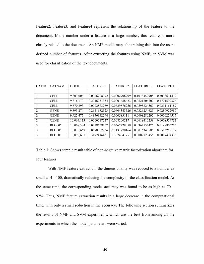
Table 7 shows a small fraction of a sample table of results of non-negative

matrix factorization algorithm for four features. The input to the NMF algorithm is

the MEDLINE training examples and output is a table of text features, the number of

which is defined by the user. For the example shown in Table 7, four features are

requested. A feature is a combination of attributes (keywords), which captures

important characteristics of the data. The numbers under the fields Feature1,

49

Feature2, Feature3, and Feature4 represent the relationship of the feature to the

document. If the number under a feature is a large number, this feature is more

closely related to the document. An NMF model maps the training data into the user-

defined number of features. After extracting the features using NMF, an SVM was

used for classification of the text documents.

Table 7: Shows sample result table of non-negative matrix factorization algorithm for

four features.

With NMF feature extraction, the dimensionality was reduced to a number as


the same time, the corresponding model accuracy was found to be as high as 70 –

92%. Thus, NMF feature extraction results in a large decrease in the computational

time, with only a small reduction in the accuracy. The following section summarizes

the results of NMF and SVM experiments, which are the best from among all the

experiments in which the model parameters were varied.

CATID CATNAME DOCID FEATURE 1 FEATURE 2 FEATURE 3 FEATURE 4 1 CELL 9,803,006 0.0006208972 0.0002706209 0.1073459908 0.3038611412 1 CELL 9,816,170 0.2046951354 0.0001488423 0.0521206707 0.4701592326 1 CELL 9,870,393 0.0002873289 0.0629876256 0.0595824569 0.0211161189 2 GENE 9,893,274 0.2641682923 0.0604343526 0.0326254629 0.0280922987 2 GENE 9,922,477 0.4856942594 0.000583111 0.0008286295 0.0000229517 2 GENE 10,064,113 0.0000017527 0.008200217 0.0618410259 0.0008524733 3 BLOOD 10,068,384 0.0218558162 0.0367229059 0.0364537425 0.0198865253 3 BLOOD 10,075,669 0.0578067936 0.1131770164 0.0016343585 0.5513259172 3 BLOOD 10,098,601 0.319241643 0.187484175 0.0007728455 0.0017494315

50

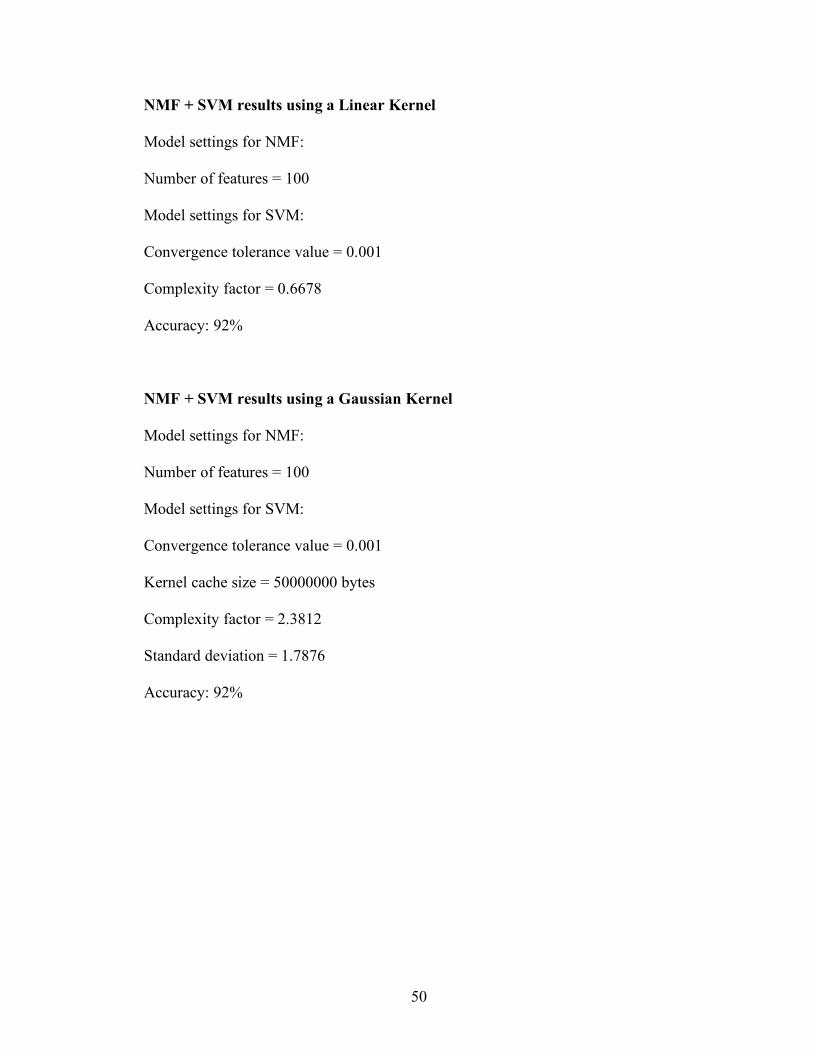
NMF + SVM results using a Linear Kernel

Model settings for NMF:

Number of features = 100

Model settings for SVM:

Convergence tolerance value = 0.001


Accuracy: 92%

NMF + SVM results using a Gaussian Kernel








Accuracy: 92%

51

NMF + SVM results using a Linear Kernel






Accuracy: 85%

NMF + SVM results using a Gaussian Kernel








Accuracy: 85%

52

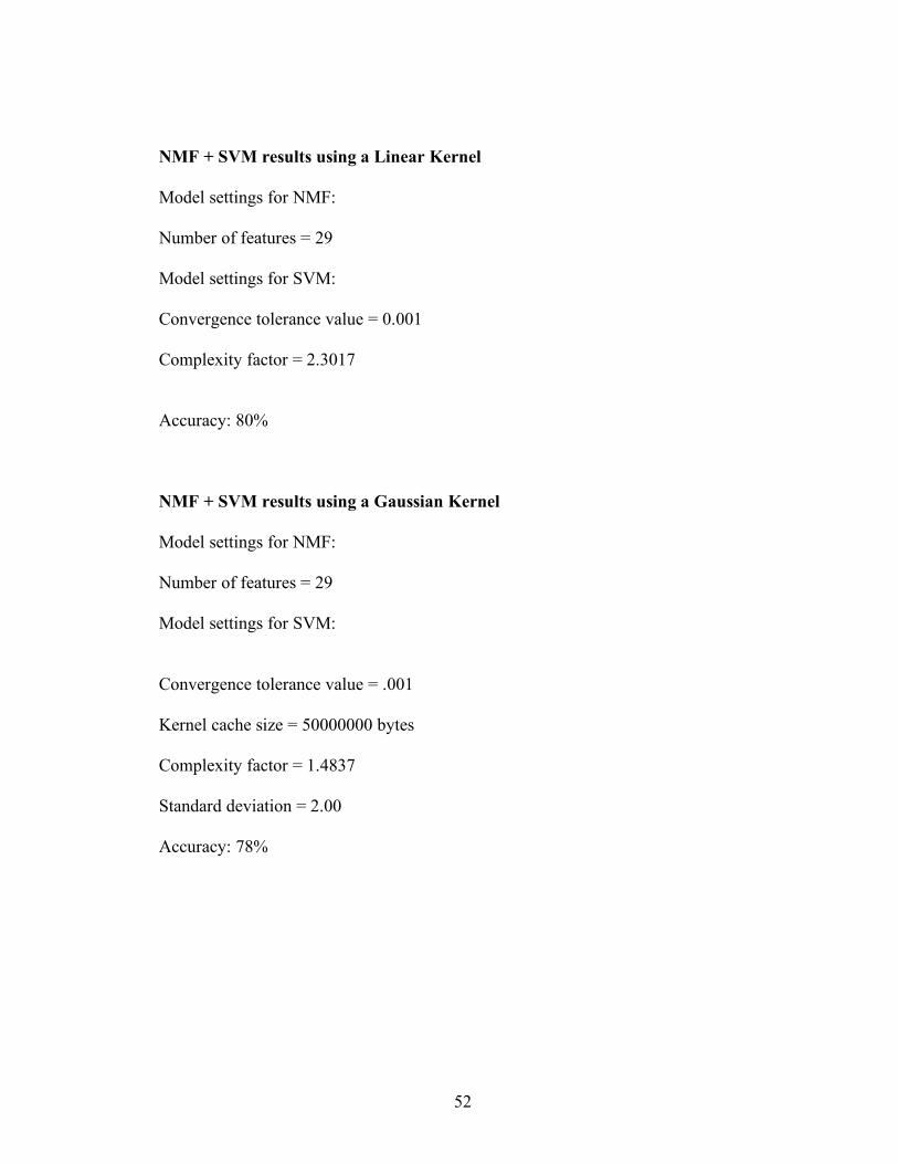
NMF + SVM results using a Linear Kernel Model settings for NMF: Number of features = 29 Model settings for SVM: Convergence tolerance value = 0.001


Accuracy: 80% NMF + SVM results using a Gaussian Kernel Model settings for NMF: Number of features = 29 Model settings for SVM: Convergence tolerance value = .001



Standard deviation = 2.00 Accuracy: 78%

53

NMF + SVM results using a Linear Kernel Model settings for NMF: Number of features = 4 Model settings for SVM: Convergence tolerance value = 0.001


Accuracy: 71% NMF + SVM results using a Gaussian Kernel Model settings for NMF: Number of features = 4 Model settings for SVM: Convergence tolerance value = .001




Accuracy: 71%

54

SUMMARY OF EXPERIMENT RESULTS

Kernel Tolerance Value Complexity

factor Accuracy

Linear 0.001 0.2 98% Gaussian 0.001 20 81% Table 8: Results Summary table for text mining with SVM only

Table 9: Results Summary table for text mining with NMF and SVM

Table 8 is a summary of results from support vector machine algorithm alone. Table 9

is a summary result of support vector machine algorithm in combination with the

non-negative matrix factorization algorithm. From the above two tables it can

concluded that for models with NMF and SVM, a relatively small number of features

yields substantially accurate results, with a large drop in the computational

complexity. The above summary tables represent the most accurate results from all

the experiments in which the model parameters were varied. On the data set, the

Kernel Number of features

Tolerance Value

Complexity factor

Accuracy

Linear 100 0.001 0.6678 92% Gaussian 100 0.001 2.3812 92% Linear 50 0.001 0.5784 85% Gaussian 50 0.001 1.4099 85% Linear 29 0.001 2.3017 80% Gaussian 29 0.001 1.4837 78% Linear 4 0.001 22.8145 71% Gaussian 4 0.001 1.2854 71%

55

dimensionality is 1617 and the SVM models achieve an accuracy of approximately

98%. With the NMF feature extraction, the dimensionality is reduced to a number as


the same time, the model accuracy is as high as 70 – 92%.

56

CHAPTER 6

CONCLUSION

Traditional text mining methods classify documents using SVM only, in

which the dimension of the attribute space is very large, resulting in large-scale

computations. The computational complexity increases rapidly as the number and the

size of the documents increases. At the same time, as demonstrated in the previous

section, models based on SVM only give high accuracy. One of the main results of

this thesis is to demonstrate that the dimension of the attribute space in the SVM

model can be reduced dramatically by employing the NMF algorithm to extract

features from the test data and using them as the attributes to build the SVM

classification model. Since the number of features is very small compared to the

initial number of attributes, the computational effort for text classification is reduced

dramatically. However, it should be expected that the reduced dimensionality would

result in a loss of classification accuracy.

The results of the previous section, summarized in Tables 8 and 9 demonstrate

that with as few as 100 features extracted from NMF, the accuracy (92%) approaches

that of the SVM only classification (98%), in which the dimension of the attribute

space of a few thousands. Table 9 also shows the rapid increase in the accuracy as the

number of features is increased. These results demonstrate that the support vector

machine algorithm and the non-negative matrix factorization algorithm, when

combined with each other, provide a powerful computational tool for text

classification, with highly reduced computational effort and very little loss of

accuracy.

57

FUTURE WORK

The work presented here can be developed further by applying it to large data

sets. Due to computer speed and memory limitations, the training and the test data set

was relatively small in this work (a few hundred documents). One of the future

directions for this work is to perform a more detailed statistical analysis of multi-

target classification on very large data sets such as the MEDLINE database.

58

REFERENCES

[1] National Library of Medicine, National Center for Biotechnology Information.

http://www.ncbi.nlm.nih.gov, (Date: 15/ 01/06).

[2] National Institutes of health, United States National Library of medicine.

http://www.nlm.nih.gov, (Date: 15/ 01/06).

[3] Joachims, T., Text Categorization with Support Vector Machines: Learning

with Many Relevant Features.

www.cs.cornell.edu/People/tj/publications/joachims_98a.ps.gz, (Date: 22/

01/06).

[4] Podowski, R. , Sample text mining application.

http://www.oracle.com/technology/industries/life_sciences/ls_sample_code.ht

ml, (Date: 17/ 01/06).

[5] Dumais, S., Using SVMs for text categorization, Microsoft research, IEEE

Intelligent Systems, 1998. www.research.microsoft.com, (Date: 21/ 03/06).

[6] Überarbeitung, J., Text mining in the Life Sciences, 26.9.2004.

http://www.coling.unifreiburg.de/research/projects/TextMining/WhitePaperV

20.pdf , (Date: 18/ 01/06).

[7] Tropp, J., An Alternating minimization algorithm for non-negative matrix

approximation.

[8] Evans, B., Non Negative Matrix Factorization, Multidimensional Digital

Signal Processing.

59

http://www.ece.utexas.edu/~bevans/courses/ee381k/projects/spring03/ , (Date:

18/ 01/06).

[9] Lee, D., Seung, H., Learning the Parts of Objects by Non-negative matrix

factorization in Nature (1999).

[10] Vapnik, V., Estimation of Dependencies Based on Empirical Data, New

York, Springer Verlag, 1982.

[11] Brank, J., Grobelnik, M., Training text classifiers with SVM on very few

positive examples, April 2003. ftp://ftp.research.microsoft.com/pub/tr/tr-2003-

34.pdf , (Date: 19/ 01/06).

[12] Liu, B., Dai, Y., Building Text Classifiers Using Positive and Unlabeled

Examples.

http://www.cs.uic.edu/~liub/publications/ICDM-03.pdf , (Date: 19/ 01/06).

[13] Oracle Corporation, Oracle data mining Concepts.

http://zuse.esnig.cifom.ch/database/doc_oracle/Oracle10G/datamine.101/b106

98.pdf, (Date: 22/ 01/06).

[14] Hearst, M., What is text mining?

http://www.sims.berkeley.edu/~hearst/text-mining.html, (Date: 22/ 01/06) .

[15] Hearst, M., Untangling text data mining.

http://www.sims.berkeley.edu/~hearst/papers/acl99/acl99-tdm.html , (Date:

25/ 01/06).

[16] Gunn, S., Support Vector Machines for Classification and Regression.

http://homepages.cae.wisc.edu/~ece539/software/svmtoolbox/svm.pdf, (Date:

05/ 02/06).

60

[17] Cherkassky, V. and Ma, Y., SVM-based Learning for Multiple Model

Estimation. http://www.ece.umn.edu/users/cherkass/Multiple_model.pdf,

(Date: 05/ 02/06).

[18] Milanova, B., Oracle data mining Support Vector Machines.

http://homepage.cs.uri.edu/faculty/hamel/dm/fall2003/boriana-

presentation.pdf , (Date: 07/ 02/06).

[19] Sassano, M., Virtual Examples for Text Classification with Support Vector

Machines.

http://acl.ldc.upenn.edu/W/W03/W03-1027.pdf , (Date: 09/ 02/06).

[20] Zhang, D., Lee, W., Question Classification using Support Vector Machines.

http://www.comp.nus.edu.sg/~leews/publications/p31189-zhang.pdf , (Date:

09/ 02/06).

[21] Pradhan, S., Ward, W., Hacioglu K., Martin, J.,

Shallow semantic parsing using support vector machines.

http://www.stanford.edu/~jurafsky/hlt-2004-verb.pdf , (Date: 10/ 02/06).

[22] Cristianini, N., Kernel Methods for Text Analysis.

http://www.support-vector.net/text-kernels.html , (Date: 20/ 02/06).

[23] Kim, H., Howland, P., Dimension Reduction in Text Classification with

Support Vector Machines.

http://jmlr.csail.mit.edu/papers/volume6/kim05a/kim05a.pdf , (Date: 03/

03/06).

[24] Tong, S, Koller, D., Support Vector Machine Active Learning with

Applications to Text Classification.

61

http://jmlr.csail.mit.edu/papers/volume2/tong01a/tong01a.pdf , (Date: 10/

03/06).

[25] Hofmann, T., Learning the Similarity of documents: An Information-

Geometric Approach to Document Retrieval and Categorization.

http://www.cs.brown.edu/people/th/papers/Hofmann-NIPS99.pdf, (Date: 20/

03/06).

[26] Boutella, M., Shena, X., Luob, J., Brownal C, Multi-label Semantic Scene

Classification.

http://www.cs.rochester.edu/u/xshen/Publications/TR813.pdf , (Date: 20/

03/06).

[27] Lauser, B., Hotho, A., Automatic multi-label subject indexing in a

multilingual environment.

http://www.aifb.uni-karlsruhe.de/WBS/aho/pub/lauserhothoecdl03.pdf, (Date:

20/ 03/06).

[28] Greevy1, E., Smeaton, A., Text Categorization of Racist Texts Using a

Support Vector Machine.

http://www.cavi.univ-aris3.fr/lexicometrica/jadt/jadt2004/pdf/JADT_051.pdf,

(Date: 21/ 03/06).

[29] PubMed website, 2004

http://www.ncbi.nlm.nih.gov/PubMed/ , (Date: 22/ 03/06).

[30] Mathiak, B., Eckstein, S., Five Steps to text mining in Biomedical Literature.

http://www.informatik.hu-berlin.de/Forschung_Lehre/wm/ws04/7.pdf, (Date:

25/ 03/06).

62

[31] Burges, C., A Tutorial on Support Vector Machines for Pattern Recognition,

data mining and Pattern Recognition.

http://research.microsoft.com/~cburges/papers/SVMTutorial.pdf, (Date: 05/

02/06).

[32] Sarkar, S., How classifiers perform on the end-game chess databases?

http://www.cs.ucsd.edu/~s1sarkar/Reports/CSE250B.pdf, (Date: 25/ 03/06).

[33] Stefan, W., James, C., Anne, D., Motivating Non-Negative Matrix

Factorizations.

http://www.siam.org/meetings/la03/proceedings/WILDstef.pdf, (Date: 09/

02/06).

[34] Stephen, I.An Improved Projected Gradient Method for Nonnegative Matrix

Factorization.

http://bugs.planetmath.org/files/papers/332/cs542_final.pdf, (Date: 09/

02/06).

[35] Amy, L., Carl, M., ALS Algorithms Nonnegative Matrix Factorization Text

Mining.

http://meyer.math.ncsu.edu/Meyer/Talks/SAS_6_9_05_NmfWorkshop.pdf,

(Date: 09/ 02/06).

63

BIBLIOGRAPHY

Amy, L., Carl, M., ALS Algorithms Nonnegative Matrix Factorization Text Mining.

http://meyer.math.ncsu.edu/Meyer/Talks/SAS_6_9_05_NmfWorkshop.pdf,

(Date: 09/ 02/06).

Boutella, M., Shena, X., Luob, J., Browna1, C., Multi-label Semantic Scene

Classification.

http://www.cs.rochester.edu/u/xshen/Publications/TR813.pdf, (Date: 20/

03/06).

Brank, J., Grobelnik, M., Training text classifiers with SVM on very few positive

examples, April 2003. ftp://ftp.research.microsoft.com/pub/tr/tr-2003-34.pdf ,

(Date: 19/ 01/06).

Brian L., Non Negative Matrix Factorization, Multidimensional Digital Signal

Processing.

http://www.ece.utexas.edu/~bevans/courses/ee381k/projects/spring03/ , (Date:

18/ 01/06).

Burges, C., A Tutorial on Support Vector Machines for Pattern Recognition, data

mining and Pattern Recognition.

http://research.microsoft.com/~cburges/papers/SVMTutorial.pdf, (Date: 05/

02/06).

Cherkassky, V., Ma, Y., SVM-based Learning for Multiple Model Estimation.

http://www.ece.umn.edu/users/cherkass/Multiple_model.pdf, (Date: 05/

02/06).

64

Cristianini, N., Kernel Methods for Text Analysis.

http://www.support-vector.net/text-kernels.html , (Date: 20/ 02/06).

Dumais, S., Using SVMs for text categorization, Microsoft research, IEEE Intelligent

Systems, 1998. www.research.microsoft.com, (Date: 21/ 03/06).

Greevy1, E., Smeaton, A., Text Categorization of Racist Texts Using a Support

Vector Machine.

http://www.cavi.univ-aris3.fr/lexicometrica/jadt/jadt2004/pdf/JADT_051.pdf,

(Date: 21/ 03/06).

Gunn, S, Support Vector Machines for Classification and Regression.

http://homepages.cae.wisc.edu/~ece539/software/svmtoolbox/svm.pdf, (Date:

05/ 02/06).

Hearst, M., Untangling text data mining.

http://www.sims.berkeley.edu/~hearst/papers/acl99/acl99-tdm.html , (Date:

25/ 01/06).

Hofmann, T., Learning the Similarity of documents: An Information-Geometric

Approach to Document Retrieval and Categorization.

http://www.cs.brown.edu/people/th/papers/Hofmann-NIPS99.pdf, (Date: 20/

03/06).

Hearst, M., What is text mining?

http://www.sims.berkeley.edu/~hearst/text-mining.html, (Date: 22/ 01/06) .

Joachims, T., Text Categorization with Support Vector Machines: Learning with

Many Relevant Features.

65

www.cs.cornell.edu/People/tj/publications/joachims_98a.ps.gz, (Date: 22/

01/06).

Kim, H., Howland, P., Dimension Reduction in Text Classification with Support

Vector Machines.

http://jmlr.csail.mit.edu/papers/volume6/kim05a/kim05a.pdf , (Date: 03/

03/06).

Lauser, B, Hotho, A, Automatic multi-label subject indexing in a multilingual

environment.

http://www.aifb.uni-karlsruhe.de/WBS/aho/pub/lauserhothoecdl03.pdf, (Date:

20/ 03/06).

Lee, D., Seung, H.S., Learning the Parts of Objects by Non-negative matrix

factorization in Nature (1999).

Liu, B., Dai, Y., Building Text Classifiers Using Positive and Unlabeled Examples.

http://www.cs.uic.edu/~liub/publications/ICDM-03.pdf , (Date: 19/ 01/06)

Mathiak, B. and Eckstein, S., Five Steps to text mining in Biomedical Literature.

http://www.informatik.hu-berlin.de/Forschung_Lehre/wm/ws04/7.pdf, (Date:

25/ 03/06).

Milenova, B, Oracle data mining Support Vector Machines.

http://homepage.cs.uri.edu/faculty/hamel/dm/fall2003/boriana-

presentation.pdf , (Date: 07/ 02/06).

National Institutes of health, United States National Library of medicine.

http://www.nlm.nih.gov, (Date: 15/ 01/06).

66

National Library of Medicine, National Center for Biotechnology Information.

http://www.ncbi.nlm.nih.gov, (Date: 15/ 01/06).

Oracle Corporation, Oracle data mining Concepts.

http://zuse.esnig.cifom.ch/database/doc_oracle/Oracle10G/datamine.101/b106

98.pdf, (Date: 22/ 01/06).

Podowski R. , Sample text mining application.

http://www.oracle.com/technology/industries/life_sciences/ls_sample_code.ht

ml, (Date: 17/ 01/06).

Pradhan, S., Ward, W, Hacioglu, K., Martin, J.H.,

Shallow semantic parsing using support vector machines.

http://www.stanford.edu/~jurafsky/hlt-2004-verb.pdf , (Date: 10/ 02/06).

PubMed website, 2004

http://www.ncbi.nlm.nih.gov/PubMed/, (Date: 22/ 03/06).

Sarkar, S., How classifiers perform on the end-game chess databases?

http://www.cs.ucsd.edu/~s1sarkar/Reports/CSE250B.pdf, (Date: 25/ 03/06).

Sassano, M., Virtual Examples for Text Classification with Support Vector Machines.

http://acl.ldc.upenn.edu/W/W03/W03-1027.pdf , (Date: 09/ 02/06).

Stefan, W., James, C., Anne, D., Motivating Non-Negative Matrix Factorizations.

http://www.siam.org/meetings/la03/proceedings/WILDstef.pdf, (Date: 09/

02/06).

Stephen, I.An Improved Projected Gradient Method for Nonnegative Matrix

Factorization.

http://bugs.planetmath.org/files/papers/332/cs542_final.pdf, (Date: 09/ 02/06).

67

Tong, S., Koller, D., Support Vector Machine Active Learning with Applications to

Text Classification.

http://jmlr.csail.mit.edu/papers/volume2/tong01a/tong01a.pdf , (Date: 10/

03/06).

Tropp, J.A., An Alternating minimization algorithm for non-negative matrix

approximation.

http://www.ece.utexas.edu/~bevans/courses/ee381k/projects/spring03/tropp/Fi

nalProjectReport.pdf, (Date: 18/ 01/06).

Überarbeitung, J., Text mining in the Life Sciences, 26.9.2004.

http://www.coling.unifreiburg.de/research/projects/TextMining/WhitePaperV

20.pdf , (Date: 18/ 01/06).

Vapnik, V., Estimation of Dependencies Based on Empirical Data, Springer Verlag

New York, 1982.

Zhang, D., Lee, W., Question Classification using Support Vector Machines.

http://www.comp.nus.edu.sg/~leews/publications/p31189-zhang.pdf , (Date:

09/ 02/06).

Documents

TEXT MINING WITH SUPPORT VECTOR MACHINES AND NON … · 2012-07-18 · 2.1 Text mining Text mining is the automatic and semi-automatic extraction of implicit, previously unknown,