Texas Water Resources Institute Annual Technical Report · PDF fileA&M University conducted an uncertainty analysis of recharge to the ... also conducted an uncertainty analysis of

Texas Water Resources InstituteAnnual Technical Report

FY 2008

Texas Water Resources Institute Annual Technical Report FY 2008 1

Introduction

The Texas Water Resources Institute (TWRI), a unit of Texas AgriLife Research, Texas AgriLife ExtensionService and the College of Agriculture and Life Sciences at Texas A&M University, and a member of theNational Institutes for Water Resources, provides leadership in working to stimulate priority research andExtension educational programs in water resources. Texas AgriLife Research and the Texas AgriLifeExtension Service provide administrative support for TWRI and the Institute is housed on the campus ofTexas A&M University.

TWRI thrives on collaborations and partnerships currently managing over 90 projects, involving more than100 faculty members from across the state. The Institute maintains joint projects with 14 Texas universitiesand three out-of-state universities; more than 30 federal, state and local governmental organizations; morethan 20 consulting engineering firms, commodity groups and environmental organizations; and numerousothers. In fiscal year 2008, TWRI obtained more than $6.1 million in funding and managed more than $20million in active projects.

TWRI works closely with agencies and stakeholders to provide research-derived, science-based informationto help answer diverse water questions and also to produce communications to convey critical information andto gain visibility for its cooperative programs. Looking to the future, TWRI awards scholarships to graduatestudents at Texas A&M University through funding provided by the W.G. Mills Endowment and awardsgrants to graduate students from Texas universities with funds provided by the U.S. Geological Survey.

Introduction 1

Research Program Introduction

Through the funds provided by the U.S. Geological Survey, the TWRI funded 10 research projects in 2008-09conducted by graduate students at Texas A&M University (8 projects) and the University of Texas at Austin(2). Additionally, through funds provided by the U.S. Geological Survey, TWRI facilitated the continuation ofthree competitive research programs at Texas A&M University.

Emily Seawright, of Texas A&M University Agricultural Economics Department, determined theeconomic impact of biological control of Arundo donax in the Rio Grande Basin.

•

Tae Jin Kim, a student in the Water Management and Hydrological Sciences Department at TexasA&M University conducted an uncertainty analysis of recharge to the Edwards Aquifer usingBayesian Model averaging scheme.

•

In the Department of Ecosystem Science And Management at Texas A&M University, SivarajahMylevaganam looked at the effect of grid sizes as subbasins on SWAT model hydrologic and waterquality predictions.

•

Texas A&M University graduate student in the Department Of Biological And AgriculturalEngineering, Deepti Puri, also conducted an uncertainty analysis of statistical model for pathogencontamination assessment in two Texas river basins.

•

Emily Martin, a student at Texas A&M University in the Soil and Crop Sciences Department, workedto develop library-independent bacterial source tracking markers for species-specific discrimination ofdeer and cattle fecal contamination in surface waters.

•

A biology student, Kranthi Mandadi, at Texas A&M University, mitigated demand for irrigated wateruse in agriculture by genetically enhancing crop plants to be productive in minimal water conditions.

•

Bo Yang, Texas A&M University student in the Department Of Landscape Architecture and UrbanPlanning used stormwater management in the Woodlands, Texas as a case study in using SWAT tocompare planning methods for neighborhoods.

•

In the Civil, Architectural and Environmental Engineering Department at the University of Texas atAustin, Eric Hersh developed an environmental flows information system for Texas.

•

Brigit Afshar, Rajan Nithya, also a student in the Civil, Architectural and Environmental EngineeringDepartment at the University of Texas at Austin, conducted microbial source tracking in drinkingwater collected from rainwater harvesting.

•

At Texas A&M University in the Ecosystem Science and Management Department, David Wattsevaluated the ecohydrology and ecophysiology of Arundo donax (giant reed).

•

Dr. Ron Griffin in the Agricultural Economics Department at Texas A&M University continued andcompleted his econometric investigation of urban water demands in the U.S. This is one of our threecompetitive research grants.

•

A second competitive research grant was conducted by Dr. Steve Whisenant in the Department ofEcosystem Science and Management at Texas A&M University and Dr. Paul Dyke at the TexasAgriLife Research Center at Temple. They are working on enhancing the Livestock Early WarningSystem (LEWS) with NASA Earth-Sun Science Data, GPS and RANET Technologies.

•

Finally, the third competitive research grant is a multi-state, international effort that involves thecollection and evaluation of new and existing data to develop groundwater quantity and qualityinformation for binational aquifers between Arizona, New Mexico, Texas and Mexico. The UnitedStates-Mexico Transboundary Aquifer Assessment Program is in the first year of the five-yearprogram.

•

Research Program Introduction 1

An Econometric Investigation of Urban Water Demand inthe U.S.

Basic Information

Title: An Econometric Investigation of Urban Water Demand in the U.S.Project Number: 2006TX253G

Start Date: 9/1/2006End Date: 12/31/2008

Funding Source: 104GCongressional District: 17

Research Category: Social SciencesFocus Category: Management and Planning, Economics, Water Use

Descriptors:Principal Investigators: Ron Griffin

Publication

An Econometric Investigation of Urban Water Demand in the U.S. 1

Progress Report Mar. 2007 – Feb. 2008 USDI/USGS Award Grant # 06HQGR0188 An Econometric Investigation of Urban Water Demand in the U.S. Ron Griffin A multilevel process of gathering historical price data has been emphasized during the past year. The website for each water utility in the sample universe (U.S. cities > 30,000 in population) has been searched for water and sewer rates back to 1995. Online archives of Codes of Ordinances have been searched for references to rate changes by ordinance or resolution. This information has been used to request documents from municipal and county government. Where less information was available, municipal sources have been queried for the desired data. Usable water rate data has been gained for some 440 communities. This does not include the desired time-series record of 11 years in all cases. Usable sewer rate data has been gained for some 330 communities. Historical water consumption volume and sectoral allocation data (residential-commercial-industrial) has been solicited, primarily at the state level . State officials were contacted for their historical records, often based on leads provided by USGS personnel. Volume information was collected for some 380 communities. Sectoral allocation by volume was collected for some 260 communities. Theoretical consideration of appropriate statistical methods has determined that the error corrections model (ECM) provides the desirable mix of shorter and longer time series treatments. The ECM allows for annual, intra-annual, and long-run elasticity parameter estimates, as well as a clear interpretation of each parameter obtained. A preliminary exploration of the integration of multiple sectors into the demand model has been devised and an abstract thereof accepted into the annual conference of the Agricultural and Applied Economics Association.

USGS Grant No. 07HQAG0077 - Enhancing the LivestockEarly Warning System (LEWS) with NASA Earth-SunScience Data, GPS and RANET Technologies

Basic Information

Title: USGS Grant No. 07HQAG0077 - Enhancing the Livestock Early Warning System(LEWS) with NASA Earth-Sun Science Data, GPS and RANET Technologies

Project Number: 2007TX318SStart Date: 6/1/2007End Date: 5/31/2010

Funding Source: SupplementalCongressional

District: 08

ResearchCategory: Climate and Hydrologic Processes

Focus Category: Drought, Agriculture, Climatological ProcessesDescriptors:

PrincipalInvestigators: Steve Whisenant

Publication

USGS Grant No. 07HQAG0077 - Enhancing the Livestock Early Warning System (LEWS) with NASA Earth-Sun Science Data, GPS and RANET Technologies1

i

Enhancing the Livestock Early Warning System (LEWS) with NASA Earth-Sun Science data, GPS and RANET Technologies:

A Collaboration with USGS/EROS

Annual Report March 2008 to February 2009

Texas Agrilife Research Texas A&M University System

2147 TAMU College Station, Texas 77843-2147

Phone: 979-845-4761

Principal Investigator: Dr. Steven G. Whisenant

Department Head Dept. of Ecosystem Science and Management

Texas A&M University College Station, Texas 77843-2126

Phone: 979-845-5579

2

Enhancing the Livestock Early Warning System (LEWS) with NASA Earth-Sun Science data, GPS and RANET Technologies:

A Collaboration with USGS/EROS

Project Description

A study was initiated in 2007 to enhance the Livestock Early Warning Systems (LEWS) decision support system (DSS) by using NASA Earth-Sun Science data by adding water resources monitoring and herd migration tools that are disseminated to pastoral communities using RANET technologies. The existing LEWS project had recognized a need to improve the existing DSS to better identify situations where water becomes a limitation to pastoral use of forage supplies in a given region. The region identified for study provides a rich environment where the technology would greatly enhance water resource monitoring and provide high impact on the national livestock sector. Monitoring the status of waterholes and rivers is important not only to the pastoralists but also for better management of the environment in terms of land degradation brought about by excessive concentration of livestock during droughts. The project was located in a transboundary site in East Africa where pastoralism is a significant component of the economy (Abule et al., 2005). The study area traverses an ecologically, ethnically and institutionally heterogeneous transect of approximately 750 kilometers, from Yabello in southern Ethiopia south through Baringo, Marsabit, Isiolo, Wajir, Mandera and Samburu districts in northern Kenya. The spatial extent of the study area is approximately 150,000 km2. This study area was chosen not only because of the international nature of its extent (i.e., Ethiopia and Kenya) but also to capture variation in ecological potential, market access, livestock mobility and ethnic diversity across the region. It is also an area characterized by a growing number of conflicts between pastoralist communities over land, water and pasture. The study area is inhabited by several main pastoral ethnic groups: the Boran, Gabbra, Somali, Rendille, Samburu and others. Climatically, southern Ethiopia is semi-arid to arid. The main pastoral group in this zone is the Boran people who are pure pastoralists. Somali clans are also found in this zone. Northern Kenya can also be characterized as semi-arid to arid with the major pastoral groups in this region being the Samburu, Turkana, Borana and Somali. All these groups are pure pastoralists and practice transhumance (i.e. the practice of moving between seasonal base camps throughout the year to optimize use of forage resources). Their livelihoods depend on herds of cattle, sheep, goats and camels for food security. They move their livestock seasonally in order to exploit grazing in areas away from their permanent settlement sites. The animals owned are used for milking, slaughtered for meat, sold for cash or bartered for other commodities. Pastoralism by definition is an extensive system of livestock production in which a degree of mobility is incorporated as a strategy to manage production over a heterogeneous landscape characterized by a precarious climate. Because of the need to take full advantage of the landscape, pastoralism is poorly fitted to the rigid structure of national and international boundaries. The pastoral strategy of mobility therefore underscores the need for a regional perspective, especially since other impacts such as resource access conflict, spread of disease and livestock rustling are side effects of pastoral mobility. For this study, we are conducting four

3

integrated activities that will provide a prototype application for arid regions in East Africa that will greatly improve the scope and effectiveness of the LEWS DSS. These four activities/objectives are as follows:

1) Characterization and verification of water resources identified with NASA Advanced Spaceborne Thermal Emission and Reflection Radiometer (ASTER), Shuttle Radar Topography Mission (SRTM) data to add a water resource mapping component to the LEWS DSS;

2) Improvement of the forage mapping component of the LEWS DSS using Moderate Resolution Imaging Spectroradiometer (MODIS) Vegetation Continuous Fields (VCF) data to extend field collected data to other unsampled areas;

3) Mapping of seasonal migration patterns and resource utilization of pastoral lands using GPS technology;

4) Operational monitoring of water resources with NASA Tropical Rainfall Measuring Mission (TRMM) data.

For each of these activities, the current status and results of each of these activities will be provided. Activity 1: Characterizing water resources with ASTER and SRTM data The main objective of this activities is to create a regional water resources inventory through the construction of a geo-database of waterholes, land cover and their drainage areas using spectral analysis of Advanced Spaceborne Thermal Emission and Reflection Radiometer (ASTER) and Moderate Resolution Imaging Spectroradiometer (MODIS) satellite imagery and applying watershed delineation tools on the 90m Shuttle Radar Topography Mission (SRTM) data. In May 2007, the USGS/EROS Data Center conducted the spectral analysis of the study area using ASTER imagery acquired during the period from 2000 to 2006. A total of 70 scenes were acquired that covered almost 85% of the study area. The analysis by USGS EROS identified 88 possible waterholes in the study area. For these, 52 were in Ethiopia, 34 in Kenya and 2 in Sudan. Only cloud free areas of the images were used to identify these waterholes, which could imply the possible existence of more waterholes that were not visible in the image due to clouds and cloud shadows. Starting in August 2007, field surveys were conducted to verify the satellite-based classifications of water holes delineated by USGS-EROS and to acquire further ancillary data for incorporation into the geodatabase on water resources in the study area. This data will include characterization of the general hydrology of the water hole (rain-fed or subsurface), flow regimes as well as technical details and locations of other water schemes such as boreholes, ponds, dry river beds, shallow wells, birkas, earth dams and other watering points, including those that were not identified during the ASTER imagery/SRTM analysis. The field inventory emphasized temporal characteristics on prevailing patterns of seasonal water availability as used by pastoralists and was be particularly focused on those regions where water becomes limiting during dry periods of the year.

4

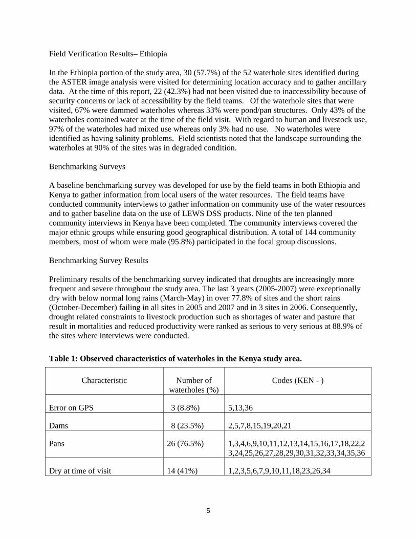
Field Verification Results– Kenya For the Kenya portion of the study area, all of the sites identified in the spectral analysis using ASTER imagery were visited and each of the 34 sites was correctly identified as being a waterhole at some point in time (e.g., Figure 1). However in three cases (waterhole # KEN-5, KEN-13, and KEN-36), the GPS coordinates did not match the location of the waterhole and necessary corrections were made. The observed waterholes were man made and classified as either pans/ponds (26 or 76.5%) or dams (8 or 23.5%) with three of the dams (KEN – 19, KEN-20, and KEN-21) having been made during the colonial era (i.e. before 1963). Nearly all (97.1%) of the waterholes were closed without an outlet channel or spillway. Only one waterhole (KEN-7) was identified as a flood hazard. In terms of size as represented by surface area, 11 (32%) were classified as small, 16 (47 %) as medium and 7 (21 %) as large. Over two-thirds of the waterholes received their recharge from different sources including river beds, or runoff ditches. Almost one third (32.4%) were recharged from underground springs and retained water throughout the year. In terms of water quality, 11 (32.4%) were saline, 22 (64.7%) had fresh water while 19 (55.9%) had low to medium turbidity. The water in 6 (17.6%) of the waterholes was for human use only whereas 16 (47.1%) were used for humans and livestock and 11 (32.4%) were used exclusively by wildlife. Waterhole KEN - 34 is not a waterhole per se, as there is no standing surface water but is in an area dotted with over 20 wells that are protected with concrete and some have reservoirs where water is stored and released to watering troughs. The initial classification of waterholes into water-like (14 or 41.2%) and clear-water (20 or 58.8%) needs to be refined in future classification analysis. Clear-water waterholes were accurately classified although 50% of them were dry at time of visit. For the water-like ones, 3 (KEN-18, KEN-23 and KEN-34) were dry, three (KEN-20, KEN-21 and KEN-22) had water from runoff, while the remaining 8 had very saline water. Of the population of waterholes visited, 8 were selected for continued monitoring using the criteria of whether they currently had water at the time of the field visit, how long they hold water, salinity status, perceived water use, and geographical distribution. The selected waterholes in Kenya were KEN-8, KEN-12, KEN-14, KEN-15, KEN-19, KEN-20, KEN-22 and KEN-36. The field team in Kenya noted that the waterholes identified from ASTER imagery represented only a small percentage (<10%) of existing open water sources (pans and dams) that occur in the Kenya study area. Table 1 provides a summary of the main characteristics of the waterholes in the Kenya study area.

Figure 1. Waterhole KEN – 24 being used by wildlife.

5

Field Verification Results– Ethiopia In the Ethiopia portion of the study area, 30 (57.7%) of the 52 waterhole sites identified during the ASTER image analysis were visited for determining location accuracy and to gather ancillary data. At the time of this report, 22 (42.3%) had not been visited due to inaccessibility because of security concerns or lack of accessibility by the field teams. Of the waterhole sites that were visited, 67% were dammed waterholes whereas 33% were pond/pan structures. Only 43% of the waterholes contained water at the time of the field visit. With regard to human and livestock use, 97% of the waterholes had mixed use whereas only 3% had no use. No waterholes were identified as having salinity problems. Field scientists noted that the landscape surrounding the waterholes at 90% of the sites was in degraded condition. Benchmarking Surveys A baseline benchmarking survey was developed for use by the field teams in both Ethiopia and Kenya to gather information from local users of the water resources. The field teams have conducted community interviews to gather information on community use of the water resources and to gather baseline data on the use of LEWS DSS products. Nine of the ten planned community interviews in Kenya have been completed. The community interviews covered the major ethnic groups while ensuring good geographical distribution. A total of 144 community members, most of whom were male (95.8%) participated in the focal group discussions. Benchmarking Survey Results Preliminary results of the benchmarking survey indicated that droughts are increasingly more frequent and severe throughout the study area. The last 3 years (2005-2007) were exceptionally dry with below normal long rains (March-May) in over 77.8% of sites and the short rains (October-December) failing in all sites in 2005 and 2007 and in 3 sites in 2006. Consequently, drought related constraints to livestock production such as shortages of water and pasture that result in mortalities and reduced productivity were ranked as serious to very serious at 88.9% of the sites where interviews were conducted.

Table 1: Observed characteristics of waterholes in the Kenya study area.

Characteristic Number of waterholes (%)

Codes (KEN - )

Error on GPS 3 (8.8%) 5,13,36

Dams 8 (23.5%) 2,5,7,8,15,19,20,21

Pans 26 (76.5%) 1,3,4,6,9,10,11,12,13,14,15,16,17,18,22,23,24,25,26,27,28,29,30,31,32,33,34,35,36

Dry at time of visit 14 (41%) 1,2,3,5,6,7,9,10,11,18,23,26,34

6

Hold water < 3 months 12 (35.3%) 1,2,3,5,6,7,9,11,18,23,26,34

Recharged from underground (all saline)

11 (32.4%) 24,25,26,27,28,29,30,31,32,33,35

Water for human use 6 (17.6%) 6,8,15,20,22,36

Water for human/livestock use 16 (47.1 %) 1,2,3,4,5,7,9,10,11,12,13,14,18,19,21,23

Water used by wildlife 11 (35.3%) 24,25,26,27,28,29,30,31,32,33,35

Potential for conflict (multiple communities)

4 (11.8%) 15, 21, 22, 36

Degraded environment 13 (38.2%) 3,4,5,6,7,8,18, 19, 20, 21, 23, 34, 36 The baseline survey results indicate that communities rely on traditional indicators of drought because most of them are not aware of or do not trust modern predictions of climate trends. Land degradation manifested as overgrazing, diminished tree cover, bush encroachment and loss of pastureland was ranked as serious to very serious in 77.8% of sites. Conflicts over access and control of resources and land ownership are common with very serious conflicts over water reported in 44.4% of sites, conflicts over pasture in 66.7% and land disputes in community, district and international border areas in 77.8% of the sites. Serious storm flooding was cited at only 2 (22.2%) of sites which are very hilly (Table 2). The temporal and spatial variation of pasture and water availability makes herd migration a key survival strategy for all communities interviewed. Most of them practice both short- and long-range movement of stock alone (with active herders) while settlements are generally permanently settled. Distances to water and pasture vary widely depending on rainfall performance compared to availability of water and pasture which are the two most important factors influencing frequency and range of migration, with water being the most critical followed by forage. Incidence and/or potential for conflict and insecurity, as well as emergence of animal diseases, also affect migration patterns. Scouts are sent out beforehand to assess the status and suitability of key resources and security situation in destination areas before migration is initiated from one grazing area the next. For all of the communities surveyed in Kenya, none were aware of the LEWS decision support system products and all indicated they would not trust external sources of early warning information. However, the general consensus was that the forage monitoring products might be useful in livestock management if and when they start receiving them in a form they can understand, to help them know if they are expecting a drought, to decide whether to sell livestock, to inform about pasture situation, assist in reducing conflicts over pasture and water, avoid overgrazing, and improve decision making on where to move animals. A modified version of the survey questionnaire was developed and will also be sent out to NGOs/institutions working in these areas to gather their views on the utility of the LEWS DSS products. Concerted efforts are needed to sensitize and train potential users about the LEWS

7

DSS in its current and enhanced forms for the post-surveys to be meaningful. The interviews of water users will continue throughout the study period to assess use of the water products developed for the LEWS DSS. A third survey has been developed for government and aid institutions in the region. This survey was conducted using online tools so that it could be easily disseminated and not require teams to conduct the survey. The survey was sent out to government and aid institutions in August 2008. Since that time, 27 individuals/organizations have taken the survey. As with the communities, the government and aid organizations were asked to rank problems related to livestock within their region according to the severity of the problem. Frequent drought and poor livestock marketing (information, facilities, and policies) were listed by the respondents as the most serious problems. Land degradation (overgrazing, bush encroachment, etc.), conflict over water, and conflict over pasture were listed as serious problems by the majority of the correspondents. Table 2: Community ranking of problems based on severity as determined through baseline community surveys in Kenya.

Problem Frequency/ percent Rank

Shortage of forage, insecurity, drought, animal diseases, poor marketing 9 (100) 1 Shortage of water 8 (88.9) 2 Land degradation, land disputes 7 (88.9) 3 Conflict over pasture 6 (66.7) 4 Conflict over water 4 (44.4) 5 Wildlife menace (predators and herbivores) 3 (33.3) 6 Strom hazard 2 (22.2) 7 Polythene, poisonous plants 1 (11.1) 8 Table 3: Government and aid organization’s ranking of problems based on severity as determined through baseline community surveys in East Africa.

Item Not serious Serious Very serious

Count of Respondents

Shortage of forage 23.8% (5) 42.9% (9) 33.3% (7) 21 Shortage of water 19.0% (4) 47.6% (10) 33.3% (7) 21 Lack of grazing land 50.0% (10) 30.0% (6) 20.0% (4) 20 Insecurity(banditry, rustling, etc) 47.6% (10) 47.6% (10) 4.8% (1) 21 Frequent drought 15.0% (3) 45.0% (9) 40.0% (8) 20 Land degradation (overgrazing, bush encroachment, etc) 5.0% (1) 60.0% (12) 35.0% (7) 20 Storm flooding 75.0% (15) 25.0% (5) 0.0% (0) 20 Conflict over water 31.6% (6) 68.4% (13) 0.0% (0) 19 Conflict over pasture 15.8% (3) 78.9% (15) 5.3% (1) 19 Land tenure/ownership 35.0% (7) 35.0% (7) 30.0% (6) 20 Animal diseases 31.6% (6) 47.4% (9) 21.1% (4) 19 Poor livestock marketing (information, facilities, policies) 30.0% (6) 30.0% (6) 40.0% (8) 20

8

Activity 2: Mapping forage baseline with MODIS Vegetation Continuous Fields

Livestock Early Warning System (LEWS) Methodology As part of the implementation of the forage monitoring simulation model for the LEWS DSS, baseline plant community information is determined by a ground sampling approach in which selected sites are visited by the LEWS teams to characterize vegetation community parameters. Simulation model runs are then parameterized for each of the sampling sites using the field information and near real-time climate data as driving variables. Modeling results for the sampling sites are then geostatistically interpolated to unsampled areas using NDVI data to produce regional maps of forage conditions. For this activity, we began the assessment on whether we could use MODIS Vegetation Continuous Fields (VCF) data to identify new monitoring sites and assist in forage model parameterization at these new sites to alleviate the need for additional field sampling.

Verification of Correspondence between VCF and LEWS DSS Data - Methods For the VCF analysis in East Africa, the MODIS VCF collection 3 data that contains proportional estimates for vegetative cover types (woody vegetation, herbaceous vegetation, and bare ground that sum up to 100%) in a 500 x 500 m pixel were used for the analysis (the most recent collection, Version 4, was not available at the time of analysis). To compare the MODIS VCF with East Africa field data, field data that were collected at 473 sites in Ethiopia, Kenya, Somalia, Uganda, and Tanzania between 1999 and 2007 (Figure 2) were used for the analysis. The field data collected for the LEWS East Africa data includes the proportion of plant species as expressed by percent basal cover of grasses, frequency of forbs, and canopy cover of shrubs/trees that existed at each site. In the LEWS DSS database, plant species are classified into functional groups of grass/grass like, forb, ground vine, climbing vine, shrub, and tree. To match the field data with VCF classification scheme, grass/grass like, forb, vines, and shrubs less than 5m were aggregated into the VCF herbaceous category, and shrubs greater than 5m and trees were combined into VCF tree category. Bare ground was derived for the LEWS DSS by subtracting the grass basal cover measured at each site from 100. The proportional estimates from the VCF images (Figure 2) were extracted using image processing software for each of three VCF cover types at each of the LEWS site locations and compared statistically to the LEWS database entries.

Verification of Correspondence between VCF and LEWS DSS Data – East Africa Results Weak correlations were found between VCF and LEWS DSS database data for herbaceous (r = 0.32) and bare ground (r = 0.43), but the correlation was especially weak for the tree proportion (r = 0.006) (Figure 4). In an examination of the proportional estimates of cover types for the VCF and the LEWS DSS data within the study area boundary in Ethiopia and Kenya, the LEWS DSS data were consistently lower than the VCF for the herbaceous proportion, especially in southern Ethiopia

9

Figure 2. Locations of field sites (left) and MODIS VCF (right) for herbaceous, tree, and bareground components in East Africa. Gray box in field site map indicates the project study area. Figure 3. Plots of proportion of cover types by MODIS VCF versus monitoring site data contained in the LEWS database in East Africa.

10

(Figure 4). The VCF data indicates that this area is dominated by relatively high proportion of herbaceous species (> 60%) while the majority of the data in the LEWS DSS indicated that the herbaceous content was less than 40%. In Northern Kenya, this could be attributed to the fact that the field data in this area were collected by visual estimates rather than field measurements due to security concerns. For Southern Ethiopia, it is harder to distinguish what the problem may be at these sites. One factor may be related to the height of trees versus shrubs. In the LEWS database, plants of the same species are classified as trees at some sites and shrubs in others and this decision was made by the field observers. Because of the cutoff for 5-m or greater height for trees in the VCF classification, an examination was conducted to determine if some of the tree species in these LEWS DSS database could be reclassified to the herbaceous category if they were less than 5 meters in height at the time of data collection. To initiate this analysis, an examination of the original datasheets for sites near Laikipia, Kenya was conducted. In doing this, inconsistencies between the original field data and the data in the LEWS DSS database were found, especially for trees and shrubs. Apparently the field collected values were modified by individuals who calibrated the model, and no records were kept of the values that were changed. The LEWS team has been working to re-enter some of the original data from various databases in each of the host countries to alleviate these discrepancies and to insure that the VCF are compared to the field collected data. At this time, it is impossible to determine if the poor correlations between the VCF data and the LEWS DSS data are the result of a true lack of correlation or if this is the result of inconsistencies in the data. In examining the data for the Laikipia sites where the original field data is available for 30 sites, the comparison between the field collected LEWS data and the VCF was generally low for both herbaceous and tree categories (r < 0.2).

Figure 4. Proportional estimates of herbaceous by MODIS VCF and LEWS DSS data. The solid square is the study area boundary.

11

Verification of Correspondence between VCF and LEWS DSS Data – Mongolia Results As another way of examining the proof of concept for using VCF data to extend the LEWS datasets, an assessment was conducted for Mongolia where the LEWS database is complete and matches the data collected in the field. Field data were collected at 297 sites in Mongolia between May 2004 and September 2006 as part of another Global Livestock-Collaborative Research Support Program (GL-CRSP) Livestock Early Warning System project. The field data include only herbaceous and bare ground as trees were not observed at the monitoring sites which are located in the southern half of the country and represent steppe, desert steppe, and steppe vegetation. Proportional estimates of cover types by VCF and field data were compared by the same manner described above for East Africa (Figure 5). There was a moderately high correlation between the VCF and field data in both herbaceous (r = 0.69) and bare ground (r = 0.69) (Figure 6, left). Field data tended to exhibit a higher proportion of the herbaceous component, on average, by 11 % (SD = 20), hence the lower estimate proportion of bare ground (Figure 6, middle and right). Although there was a low correlation between the herbaceous proportion of VCF and monitoring site data in East Africa, the observed moderately high correlation between the two data sources in Mongolia provided an opportunity to test the use of VCF-derived parameters for deriving simulation model (PHYGROW) inputs for new sites. A series of PHYGROW model simulations was derived using VCF-derived herbaceous proportion developed for 167 independent validation sites not included in the correlation analysis. Herbaceous biomass was collected at each of these 167 sites as part of the initial LEWS validation in Mongolia. To derive the model parameters for the new sites, regression was used to predict herbaceous proportion using VCF data as an independent variable with the calibration data from the 297 monitoring sites. To bind the proportion values between zero and one, a generalized linear model with a logit link function was used to predict the herbaceous proportion at the independent validation sites using the regression. The PHYGROW model requires plant composition, soil type, and stocking rate as input parameters for each monitoring site. For each of the new validation sites, it was assumed that each site had the same plant species composition as its nearest calibration site. To identify the soil type, two different methods were tested: (1) assume that the soil type at each new validation site was the same as its nearest calibration site (method 1), (2) use soil type as designated by the Mongolia national soil survey map (method 2). Figure 5. Locations of field sites (left) and MODIS VCF estimates for herbaceous (middle) and bare ground (right) in Mongolia.

12

Figure 6. Plots of proportion of cover types by MODIS VCF vs. field data in Mongolia (left) and box plot of difference in proportions (field data – MODIS VCF) (right). The current method used in Mongolia to predict herbaceous biomass, geostatistical interpolation (cokriging) of PHYGROW model output for the 297 monitoring sites are combined with the NASA GIMMS NDVIg product to predict herbaceous biomass at unsampled sites. A comparison was conducted to assess the differences in biomass predicted by cokriging at the independent validation sites and that predicted using the VCF for both Method 1 and Method 2 (Table 4). The results did not indicate an improvement in biomass prediction as compared to the current interpolation method using cokriging. The correlation coefficient between predicted and clipped biomass was reduced from 0.52 to 0.17 for Method 1 and 0.21 for Method 2. Root Mean Square Error of Prediction (RMSEP) and mean absolute error (MAE) increased under both methods (7.41 and 9.07 kg/ha for RMSEP, and 81.71 and 83.1 kg/ha for MAE for Method 1 and 2, respectively) (Table 4). Additional analyses are currently being conducted to assess reasons for the lower performance of the VCF methods and to examine alternative ways of improving performance. Table 4. Summary of validation with three methods: cokriging of calibration sites using NDVI as a covariate (cokriging), and VCF-based herbaceous proportion with the same soil type as the nearest calibration sites (method 1) and with the soil type identified using a national soil survey map in Mongolia (method 2).

Method

Correlation

Coefficient (r)

Root Mean Square Error

of Prediction (RMSEP)

(kg/ha)

Mean absolute

error (MAE)

(kg/ha)

Cokriging 0.52 16.32 127.71

Method 1 0.17 23.73 196.87

Method 2 0.21 25.39 210.81

13

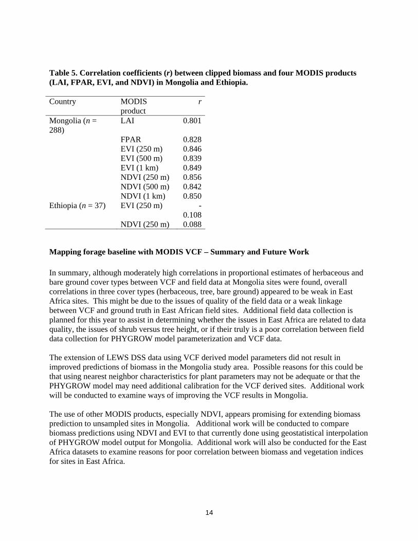
Comparisons of LEWS DSS data to other MODIS datasets The MODIS VCF version 3, which represents conditions pre-2001, is the most recent VCF dataset that predicts the herbaceous component. The more recent data in Version 4, currently only provides estimates of the proportion of trees on the landscape. Because of the lack of recent updates of the herbaceous component for the VCF, other MODIS products that are updated more frequently were examined for use in extending LEWS DSS datasets. These products included the Fraction of Photosynthetically Active Radiation (FPAR), Leaf Area Index (LAI), the Enhanced Vegetation Index (EVI), and the Normalized Difference Vegetation Index (NDVI). For an initial analysis, the linkage between these MODIS products and clipped herbaceous biomass was examined. Composite images for each product were acquired from the LP-DAAC for the date periods in which biomass was sampled. The product data were extracted for the location of each of the LEWS monitoring sites using image processing software. Field data in Mongolia were first examined since the biomass data collection is more extensive than in East Africa. Herbaceous biomass data collected in Mongolia during 2004 through 2005 and the collocated data for the four MODIS products (LAI, FPAR, EVI, and NDVI at each available resolution) were examined using correlation analysis. For the LAI and FPAR data, 88 out of 288 sites (30% of the sites) had only fill values for LAI and FPAR due to condition of barren, desert, or very sparse vegetation at sample sites. A high correlation between clipped biomass and both LAI (r = 0.80) and FPAR (r = 0.83) was observed for the sites in which LAI and FPAR values could be extracted (Table 5). Correlation between clipped biomass and EVI and NDVI ranged 0.84 to 0.85 and 0.85 to 0.86 respectively. Of the two vegetation indices, NDVI had overall stronger correlation with clipped biomass than EVI. With NDVI, the correlation was slightly stronger with 250 m data compared to 500 m and 1 km resolution data. Because it appeared that the Vegetation Indices data were more promising than the LAI and FPAR datasets, a correlation analysis was conducted using herbaceous biomass data that was collected at 37 sites in Ethiopia in 2007. In this analysis, poor correlations with both EVI (r = -0.11) and NDVI (r = 0.15) were found (Table 5). This lack of correlation may be related to the incidence of shrubs for which biomass was not measured at the monitoring sites. These shrubs may have inflated the NDVI values in relation to the herbaceous biomass thus reducing the correlations. Analyses are currently being conducted to examine the influence of shrubs on these correlations.

14

Table 5. Correlation coefficients (r) between clipped biomass and four MODIS products (LAI, FPAR, EVI, and NDVI) in Mongolia and Ethiopia. Country MODIS

product r

Mongolia (n = 288)

LAI 0.801

FPAR 0.828 EVI (250 m) 0.846 EVI (500 m) 0.839 EVI (1 km) 0.849 NDVI (250 m) 0.856 NDVI (500 m) 0.842 NDVI (1 km) 0.850Ethiopia (n = 37) EVI (250 m) -

0.108 NDVI (250 m) 0.088

Mapping forage baseline with MODIS VCF – Summary and Future Work In summary, although moderately high correlations in proportional estimates of herbaceous and bare ground cover types between VCF and field data at Mongolia sites were found, overall correlations in three cover types (herbaceous, tree, bare ground) appeared to be weak in East Africa sites. This might be due to the issues of quality of the field data or a weak linkage between VCF and ground truth in East African field sites. Additional field data collection is planned for this year to assist in determining whether the issues in East Africa are related to data quality, the issues of shrub versus tree height, or if their truly is a poor correlation between field data collection for PHYGROW model parameterization and VCF data. The extension of LEWS DSS data using VCF derived model parameters did not result in improved predictions of biomass in the Mongolia study area. Possible reasons for this could be that using nearest neighbor characteristics for plant parameters may not be adequate or that the PHYGROW model may need additional calibration for the VCF derived sites. Additional work will be conducted to examine ways of improving the VCF results in Mongolia. The use of other MODIS products, especially NDVI, appears promising for extending biomass prediction to unsampled sites in Mongolia. Additional work will be conducted to compare biomass predictions using NDVI and EVI to that currently done using geostatistical interpolation of PHYGROW model output for Mongolia. Additional work will also be conducted for the East Africa datasets to examine reasons for poor correlation between biomass and vegetation indices for sites in East Africa.

15

Activity 3: Mapping seasonal migration patterns with GPS technology Under this activity, the movement patterns of pastoralists and their livestock herds in response to changing forage and water supply will be tracked using GPS tracking technology. This will allow comparisons of the various communities’ mobility and grazing management behaviors to the prevailing forage and water resource conditions and provide insights that will allow improvement in the LEWS information flow in the target region. The outcome of this activity will be to develop practical recommendations that pastoral communities and land managers can use to optimally exploit the forage and water resources and improve the productivity in these arid and semi-arid rangelands. The pastoralist groups that will have GPS equipment will be representative of the pastoral communities in each of the countries representing pastoralists’ mobility patterns, ecological and resource potential, ethnic representation, wealth status/herd size strata among other factors such as accessibility. These representative groups were identified through rapid appraisal surveys conducted by the field teams in Kenya and Ethiopia. GPS’s have been given to select herder groups and individuals were trained by the LEWS team in GPS data collection procedures. Collectors are asked to log their positions at watering, grazing, and resting points. The GPS’s are being collected periodically by the field teams to replace batteries and to download data. Mobility and other relevant data will be determined from the downloaded data and added to the main database at the base of operations of the project in each country. The data collection will continue into the summer of 2009 and be analyzed during the third year of the study. Activity 4: Operational monitoring of water resources with TRMM In this activity, it is planned that new water resources monitoring products will be added into the LEWS DSS. These new products will be essential for monitoring the conditions of water resources that are vital in decision making by the user community of herders. In particular, daily water availability monitoring products will be developed for individual waterholes, and daily river flow hydrographs of major streams along the migration routes will be produced. The majority of tasks for this activity are being conducted by the USGS/EROS team in association with the ASTER imagery analysis under Activity 1. USGS-EROS has developed daily rainfall estimates subsetted from the NASA TRMM dataset for Africa. A modeling framework for modeling daily catchment runoff for the contributing areas around waterholes using the TRMM dataset has been developed and is fully operational. Daily water level changes (whether positive or negative) are being estimated for sixteen (16) major waterholes identified under Activity 1 of this study using similar techniques by Senay and Verdin (2004). The Texas AgriLife Research team has worked with USGS and their subcontractor South Dakota State University to develop a web portal for displaying the water monitoring activities. The website can be viewed at http://watermon.tamu.edu. This website offers users the ability to monitor and download waterhole depth information from 1998 to present. The sixteen representative waterholes in the region are being operationally monitored (with a day lag) for variations in waterhole depths. The site provides the current status of depths for each waterhole

16

(daily depth variation information) which would enable pastoral communities to make appropriate decisions on their migratory movements in search of water and forage. It also allows users to examine the median water levels along with past years data (Figure 7).

Figure 7. Depth dynamics for a 60 day period at waterhole KEN-15 as indicated by the USGS water depth simulation modeling using TRMM rainfall data as displayed on the http://watermon.tamu.edu website. The top graph indicates the depth of water as estimated for current conditions (2009), last year’s (2008) depth, and the median depth since 1998. Rainfall and evaporation are also given.

17

References Abule, E., H.A Snyman and G.N Smit. 2005. Comparisons of pastoralists’ perceptions about rangeland resource utilisation in the Middle Awash Valley of Ethiopia. J. Environ. Manage. 75, 21–35. Senay, G.P. and J.P. Verdin, 2004. Developing index maps of water-harvest potential in Africa. Applied Engineering in Agriculture, American Society of Agricultural Engineers, 20(6): 789-799.

Economic Impacts of Biological Control of Arundo donax inthe Rio Grande Basin

Basic Information

Title: Economic Impacts of Biological Control of Arundo donax in the Rio Grande BasinProject Number: 2008TX303B


Funding Source: 104BCongressional

District: 15, 25, 23, 28

Research Category: Biological SciencesFocus Category: Economics, Invasive Species, Surface Water

Descriptors: NonePrincipal

Investigators:Emily K Seawright, John A Goolsby, Ron Lacewell, M Edward Rister, Allen WSturdivant

Publication

Seawright, E.K., M.E. Rister, R.D. Lacewell, A.W. Sturdivant, and J.A. Goolsby. February 8-12,2009. “Economic Implications of Biological Control of Giant Reed on the Rio Grande.” inProceedings of the 2009 USDA-CSREES National Water Conference. St. Louis, MO. (abstract only)

1.

Seawright, E.K., M.E. Rister, R.D. Lacewell, A.W. Sturdivant, J.A. Goolsby, and D.A. McCorkle.January 31-February 3, 2009, “Biological Control of Giant Reed (Arundo donax): EconomicAspects.” in Proceedings of the 2009 Southern Agricultural Economics Association Annual Meeting.Westin Peachtree Plaza. Atlanta, GA.

2.

Seawright, E.K., M.E. Rister, R.D. Lacewell, J.A. Goolsby, and A.W. Sturdivant. July 22-24, 2008.“Biological Control of Giant Reed Along the Rio Grande: An International Boundary.” inProceedings of ‘International Water Resources: Challenges for the 21st Century and Water ResourcesEducation’ Universities Council on Water Resources Annual Meeting. Durham, NC.(abstract only)

3.

Seawright, E.K., M.E. Rister, R.D. Lacewell, A.W. Sturdivant, J.A. Goolsby, and D.A. McCorkle.January 8, 2009. “Economic Implications of Biological Control for Arundo donax along the RioGrande.” Arundo donax Biological Control Team Meeting. Laredo, TX.

4.

Seawright, E.K., M.E. Rister, R.D. Lacewell, A.W. Sturdivant, and J.A. Goolsby. December 4, 2008.“Giant Reed: Economic Implications of Biological Control Along the Rio Grande.” AnnualConference of the Texas Plant Protection Association. College Station, TX.

5.

Seawright, E.K., M.E. Rister, R.D. Lacewell, A.W. Sturdivant, and J.A. Goolsby. June 26, 2008."Progress on Economic Report for the USDA-ARS Biological Control of Arundo donax." Arundodonax Biological Control Team Meeting. College Station, TX.

6.

Seawright*, E.K., C.N. Boyer*, S.R. Yow*, A.J. Leidner*, M.E. Rister, R.D. Lacewell, and A.W.Sturdivant [* 1st author]. March 4, 2008. “Student Research – the Rio Grande Basin Initiative.”Meeting of Agricultural Economics Faculty Retirees. College Station, TX.

7.

Seawright, E.K. Forthcoming in August 2009. “Economic Implications for Biological Control ofArundo donax.” Master of Science Thesis. Department of Agricultural Economics, Texas A&MUniversity. College Station, Texas.

8.

Economic Impacts of Biological Control of Arundo donax in the Rio Grande Basin 1

1

Report

Title: Economic Impacts of Biological Control of Arundo donax in the Rio Grande Basin

Project Number: 40770

Primary PI: Emily Kaye Seawright, B.S., Texas A&M University

Other PIs: M. Edward Rister Ronald D. LacewellDean A. McCorkleJohn A. GoolsbyAllen W. Sturdivant

Abstract

Problem and Research ObjectivesArundo donax, or giant reed, is a large, bamboo-like plant that is native to Spain and is thrivingin the Mediterranean climate of the Rio Grande [River] in Texas (Goolsby and Moran 2009). Itgrows 6-8 meters (18-24 feet) tall (Bell 1997), consumes large quantities of water (exceedingfour acre-feet per year) (Iverson 1994), and has invaded several thousand acres of the Rio Granderiparian (Yang 2008). With rising concern of increased water demands in the region, the UnitedStates Department of Agriculture-Agricultural Research Service (USDA)ARS) is investigatingfour insects, i.e., Tetramesa romana (wasp), Rhizaspidiotus donacis (scale), Cryptonevra spp.(fly) and, and Lasioptera donacis (leafminer), for their ability and appropriateness to perform asbiological control agents for Arundo donax (Goolsby 2008). This study examines the economicimplications of using these biological control agents along the Rio Grande. Included in theeconomic estimates are (1) estimating the value of the water saved due to the reduction ofArundo donax, (2) a benefit-cost analysis, (3) an economic impact analysis for the region, and (4)an estimate of the per-unit cost of water saved.

MethodologyThe expansion of giant reed is projected over a 50-year planning horizon (2009 through 2058) todefine an uncontrolled baseline scenario along the Rio Grande in Texas. This baseline ismodified to reflect the efficacy of the introduced insects. The net amount of water saved isdetermined by estimating reduced water consumption associated with the control of giant reed.

Municipalities in South Texas have first priority in the allocation of water and as such, will notbe the user of water saved from the control of giant reed. Consequently, water saved will go toagriculture where irrigated acres can be increased. This suggests that agriculture is the residualuser in the Lower Rio Grande Valley of Texas and is thus, the primary beneficiary of the savedwater from the Arundo donax biological control program.

2

Crop enterprise budgets are examined to estimate the value of saved water used for agricultural irrigation. Benefits of controlling giant reed are estimated using the low- and high-marginalvalue composite acre with market prices for crops and alternatively, using the low- and high-marginal value composite acre with normalized prices that exclude any impacts of farm program(social accounting) for crops. Using economic and financial tools, a benefit-cost analysis isdeveloped based on reducing the expansion rate of the plant. Sensitivity analyses are performedfor the benefit-cost ratios to account for uncertainty associated with the variables in the analysis. The economic impact is estimated using projected gross revenue changes associated with Arundocontrol and applying economic and employment multipliers from the IMPLAN model developedby Minnesota ImPlan Group, Inc. Finally, the estimates for the per-unit cost of water saved arederived using financial analysis and tools of capital budgeting.

Principal FindingsThe deterministic analyses using composite acre values calculated with market prices reveal aregional present value of farm-level benefits ranging from $97.8 million to $159.9 million. Social benefits, using composite acre values calculated with normalized prices, range from $72.4million to $145.7 million, with an associated benefit-cost ratio ranging from 4.35:1 to 8.74:1. This suggests social returns of $4.35 to $8.74 per dollar of government expenditure.

Sensitivity analyses are done to provide insight into results and to identify more robustimplications. Ranges in Arundo water use are the basis of the sensitivity analyses and are variedagainst ranges for the efficacy of the Arundo biological control program, as well as for native(replacement) species water use, Arundo expansion rate after control, discount rate on dollars,value of water, and the cost of the biological control program. When varying the efficacy of thebiological control program with the ranges in Arundo water use, the benefit-cost ratio rangesfrom 1.55:1 to 7.70:1. Further sensitivity analyses varying Arundo water use with the other listedvariables identify additional ranges in estimated levels of expected benefits for the program.

The impact analysis revealed a range for 2009 of $0.011 million to $0.030 annually in value-added, $0.022 million to $0.045 million annually in economic output, and no new jobs to theregion. In 2035, annual value-added ranges from $6.0 million to $16.0 million, economic outputranges from $12.1 million to $24.4 million, and 267-477 new jobs to the region. In 2058, theeconomic impact ranges from $11.2 million to $29.9 million annually for value-added, $22.5million to $45.4 million annually in economic activity created, and 498 to 888 new jobs for theregion.

The per-unit cost estimate for the biological control program reveal a cost per acre-foot of waterof $44.42, and a cost per thousand gallons of water of $0.1363. These cost values arecomparable to and less than many other projects designed to “create” or conserve water in theTexas Lower Rio Grande Valley (Sturdivant et al. 2009).

3

SignificanceThe positive benefit-cost ratios in the analyses indicate the project will produce positive netbenefits relative to the costs of the program. Additionally, the results of the impact analysesindicate this project will have positive economic implications for the Texas Lower Rio GrandeValley region with increased value-added production, increased economic activity, and increasedjobs. Additionally, the per-unit cost of the saving water through the Arundo biological controlprogram is comparable to current projects designed to conserve water in the region. Overall, theUSDA-ARS, Weslaco, Texas Arundo donax biological control project creates benefits and willhave a positive economic impact to the Texas Lower Rio Grande Valley region.

References Cited

Bell, Gary P. 1997. Ecology and Management of Arundo donax, and Approaches to RiparianHabitat Restoration in Southern California. In Brock, J. H., Wade, M., Pysek, P., andGreen, D. (Eds.): Plant Invasions: Studies from North America and Europe. BlackhuysPublishers, Leiden, The Netherlands, pp. 103-13.

Goolsby, John A. 2008. Entomologist. Personal Communication. USDA-ARS. Weslaco, TX,18 April, 2008.

Goosby, John A. and Patrick Moran. 2009. “Host range of Tetramesa romana Walker (Hymenoptera: Eurytomidae), a potential biological control of giant reed, Arundo donaxL. in North America.” Biological Control (2009), doi: 10.1016/j.biocontrol.2009.01.019.

Iverson, M.E. 1994. The impact of Arundo donax on water resources. November 1993. Arundodonax workshop proceedings, pp. 19-25. Ontario, CA.

Minnesota ImPLAN Group, Inc. 2006. Multiplier Data. Stillwater, Minnesota: MinnesotaIMPLAN Group, Inc.

Sturdivant, A.W. 2009. Extension Associate (Economist). Texas AgriLife Extension Service. Weslaco, TX. Personal Communications.

Yang, Chenghai. 2008. Personal E-mail. United States Department of Agriculture-AgriculturalResearch Service. Weslaco, TX, October 7, 2008.

Uncertainty Analysis of Recharge to the Edwards Aquiferusing Bayesian Model Averaging Scheme

Basic Information

Title: Uncertainty Analysis of Recharge to the Edwards Aquifer using Bayesian ModelAveraging Scheme

Project Number: 2008TX304BStart Date: 3/1/2008End Date: 2/28/2009


District: 17

Research Category: Ground-water Flow and TransportFocus Category: Groundwater, Models, Water Quantity

Descriptors:Principal

Investigators: Champa Joshi, Binayak Mohanty

Publication

Uncertainty Analysis of Recharge to the Edwards Aquifer using Bayesian Model Averaging Scheme1

1

Uncertainty Analysis of Recharge to the Edwards Aquifer using Bayesian Model

Averaging Scheme

Champa Joshi

1. Introduction

Appropriate estimation of recharge is essential to avoid the excessive depletion as

well as for the proper management of the available groundwater resources in a

watershed/basin. Proper assessment of recharge also helps in planning and designing Best

Management Practices (BMPs) to meet the existing and future water demands in a region.

Recharge is basically the excess amount of precipitation entering the subsurface after

accounting for the losses due to ET, overland flow, and surface runoff. There are a lot of

uncertainties involved in quantifying the exact amount of recharge. These uncertainties

are caused by numerous factors. The objective of the study is to assess the uncertainty

involved in estimating the amount of recharge entering the Edwards Aquifer which

exhibits karst geology. Currently, the Hydrologic Simulation Program – Fortran (HSPF)

model developed by Crawford and Linsley (1966) is widely used to compute the recharge

entering the Edwards Aquifer. HSPF is a comprehensive, conceptual, continuous

watershed simulation model designed to simulate all the water quantity and water quality

processes that occur in a watershed, including sediment transport and movement of

contaminants. It is usually classified as a lumped model. Although data requirements are

extensive, EPA recommends its use as the most accurate and appropriate management

tool available for the continuous simulation of hydrology and water quality in

watersheds. But every model has its own strength and limitations depending upon its

governing equations, model structure, and spatial and temporal data/grid resolution. All

2

these factors (i.e., input parameter, forcings, and model structure) lead to uncertainties in

model output. Therefore, it would be worthwhile to explore the possibility of using other

hydrologic models (e.g., NOAH, SWAP, and VIC) for computing the recharge and

thereby evaluating the uncertainty involved in the process. A multi-model combination

using Bayesian model averaging (BMA) scheme is expected to further improve the

predictions by better addressing the model structural uncertainty. Therefore, based on our

research motives, it was planned to initially conduct the study in the Trinity River basin,

and later use the gained knowledge and expertise to assess the uncertainty associated with

recharge estimates in the Edwards Aquifer region. As Edwards Aquifer has a more

complex hydrology due to its karst geology, it is wise to proceed in a stepwise manner to

understand the contribution of model complexity to the recharge uncertainty.

2. Study site and data description

2.1 Study Area

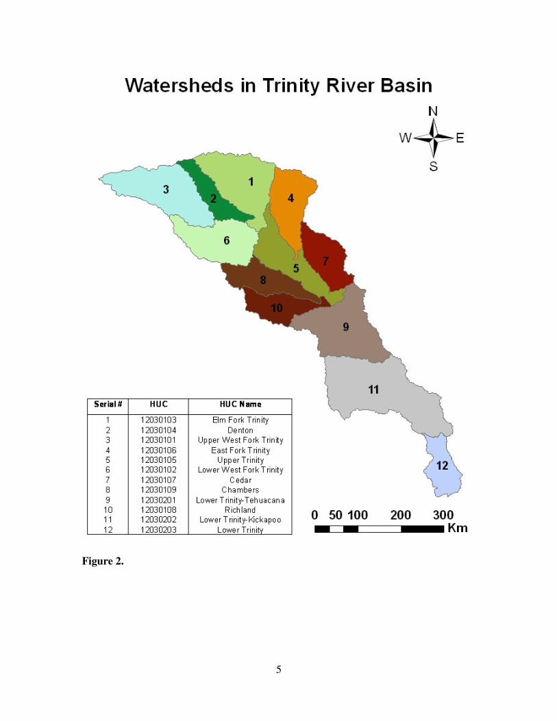
Figure 1 shows the study area, i.e., the Trinity River basin. The basin consists of

12 watersheds shown in Figure 2 along with their HUC (Hydrological unit code) numbers

and names. The 710-mile long Trinity River that flows entirely within the State of Texas

is highlighted in Figure 1. Following River Kuskokwim in Alaska, Trinity is the second

longest river which flows entirely within one state (i.e., Texas) in U.S.A.. The Trinity

River rises in extreme north Texas, a few miles south of the Red River, with its

headwaters separated from the Red River basin by the high bluffs lying south of the Red

River. The river has four forks, namely, the Clear Fork, the Elm Fork, the West Fork, and

the East Fork. The West Fork flows eastward through the city of Fort Worth and Lake

3

Worth. On the other hand, the Clear Fork flows southeastward in its upper part, then

northeastward through Fort Worth. The West Fork and the Clear Fork then meet near

downtown. The Elm Fork flows south from near Gainesville and east of Denton. As those

two rivers enter Dallas, they merge to form the Trinity River proper. The East Fork starts

near McKinney and joins Trinity, southeast of the city of Dallas. The Trinity River then

flows in the south-east direction from Dallas across a fertile floodplain and pine forests of

eastern Texas. The River further flows south to join the Trinity Bay (which is the

northeastern portion of the Galveston Bay), east of Houston. The various tributaries of

the Trinity River are: Bachman Branch, Cedar Creek, Johnson Creek, Red Oak Creek,

Richland Creek, and White Rock Creek.

There are 22 major reservoirs which provide nearly 90% of the surface water used

in the Trinity River basin. The reservoirs considerably impact the streamflow and water

quality in the basin. Water from the reservoirs is used mainly for water supply and flood

protection, and relatively low amount is use for irrigation. Aquifers outcrop in all or parts

of the Western and Eastern Cross Timbers, Eastern Timberlands, Texas Claypan, and

Coastal Prairie and Marsh. In smaller towns and rural areas, mostly ground water is used

for municipal and domestic purposes.

Precipitation and streamflow best characterize the hydrologic conditions

prevailing in the Trinity River Basin. Precipitation varies considerably across the basin

and is mostly in the form of rain. The average annual rainfall varies between ~27 inches

in the north-west to ~52 inches in the south-east. Streamflow varies in proportion to the

rainfall and the watershed size, except downstream from reservoirs and point sources.

4

Figure 1.

5

Figure 2.

6

2.2 Input Data

This section briefly describes the various forcings used for conducting the study. The

input forcings mostly consist of the remote sensing data available for the Trinity River

basin. All the remote sensing data were collected for the year 2005 and were processed

accordingly (using ArcGIS and MATLAB) to retrieve the desired data format. The

resulting daily spatially distributed hydro-climatic datasets were used for running the

various hydrology models to estimate the recharge. The data were resampled to a cell size

of 8,000 m X 8,000 m and projected to the WGS84 UTM Zone 14 coordinate system as

shown in Figures 3 and 4.

DEM: The GTOPO30 data (resolution: 1,000 m X 1,000 m) available from the United

States Geological Survey (USGS) website was used for obtaining the elevation and slope

information of the Trinity River basin. Figure 3a shows the elevation varying between a

maximum of 399 m in the extreme north to a minimum of 1 m in the extreme southern

part of the basin. The DEM-derived slope information is given in Figure 3b. Thus, the

topography of the basin mainly consists of eight major regions: the North Central Prairie,

the Grand Prairie, the Blackland Prairie, the Eastern Timberlands, the Coastal Prairie and

Marsh, the Bottomlands, the Texas Claypan, and the Western and Eastern Cross Timbers.

Vegetaion: The Leaf Area Index (LAI) obtained from the MODIS (Moderate Resolution

Imaging Spectroradiometer) satellite is used in this study. The original resolution of the

data is 1,000 m X 1,000 m. Figure 3c shows a sample snapshot of 8-day composite LAI

for the period from 5th

to 7th

August, 2005.

7

Precipitation: For precipitation information, the Nexrad-based (resolution: 4,000 m X

4,000 m) data set is used. A sample snapshot of precipitation on 6th

June, 2005 (see

Figure 3d) shows the rainfall varying between 0 to 44.2 mm.

Soil: The STATSGO-based soil texture map (resolution: 1,000 m X 1,000 m) shown in

Figure 4 illustrates that the soil type varies greatly within the Trinity River basin. Table 1

gives the dominant soil texture information corresponding to the various soil MUID.

Based on the soil textural classes, the soil hydraulic properties given by Carsel and

Parrish, 1988 is used in the study (see Table 2).

Meteorological Forcings: The atmospheric forcing data such as air temperature, wind

speed, solar radiation, relative humidity, etc. which is spatially homogeneous at large

scale is obtained from the 40 years reanalysis products of North America Regional

Reanalysis (NARR). The NARR data was disaggregated and averaged to ~8,000 m for

modeling purposes.

8

Figure 3.

9

Figure 4.

10

Table 1.

Soil Dominant Soil Dominant Soil Dominant

MUID Soil texture MUID Soil texture MUID Soil texture

8208 CL 8393 SL 8613 S

8229 SIL 8400 SL 8614 SL

8232 SL 8404 S 8618 C

8233 C 8406 CL 8622 CL

8234 C 8410 SL 8633 SL

8235 SIC 8411 L 8639 CL

8242 C 8420 SL 8649 SL

8248 SIL 8421 SL 8650 SL

8250 SL 8425 C 8689 SL

8253 CL 8434 C 8697 C

8258 SL 8435 C 8712 SL

8259 SL 8445 C 8716 SL

8263 SL 8446 SIL 8729 L

8281 C 8450 C 8765 SL

8284 SL 8462 SL 8769 C

8317 L 8468 S 8777 SIC

8318 L 8469 SL 8778 SIC

8320 SL 8470 L 8798 C

8339 S 8479 SL 8805 CL

8340 SIL 8495 S 8807 SL

8360 SL 8570 SL 8814 S

8377 SICL 8582 SL 8815 SL

8378 SL 8587 S 8817 SL

8385 SL 8593 CL 8821 SL

8392 SICL 8612 S 8825 SL

Table 2.

(Hydraulic properties as per Carsel and Parrish, 1988)

Class No. Soil Texture ClassClass Abbrev. θr θs α (1/cm) n Ksat (m/day)

1 Sand S 0.045 0.43 0.145 2.68 7.128

2 Loamy Sand LS 0.057 0.41 0.124 2.28 3.502

3 Sandy Loam SL 0.065 0.41 0.075 1.89 1.061

4 Silt Loam SiL 0.067 0.45 0.02 1.41 0.108

5 Silt Si 0.034 0.46 0.016 1.37 0.06

6 Loam L 0.078 0.43 0.036 1.56 0.249

7 Sandy Clay Loam SCL 0.1 0.39 0.059 1.48 0.314

8 Silty Clay Loam SiCL 0.089 0.43 0.01 1.23 1.68

9 Clay Loam CL 0.095 0.41 0.019 1.31 0.062

10 Sandy Clay SC 0.1 0.38 0.027 1.23 0.028

11 Silty Clay SiC 0.07 0.36 0.005 1.09 0.005

12 Clay C 0.068 0.38 0.008 1.09 0.048

11

3. Method of Analysis

The methodology used in this study will include three different hydrologic

models used individually to compute the recharge and assess the associated uncertainty.

A multi-model combination using BMA scheme will also be employed to reduce the

uncertainty and improve the recharge predictions using multiple model outputs. While

estimating the amount of recharge using different models, uncertainty can arise mainly

due to the following reasons, namely: (1) Parameter uncertainty, (2) Input data

uncertainty (e.g., model forcings), and (3) Model structural uncertainty (e.g.,

dimensionality of the model – 1D/2D, type of model – process-based / conceptual, etc.).

The cumulative effects of these uncertainties lead to an inaccurate estimation of the

variable of interest, i.e., recharge.

In this study, three different hydrologic models, namely, NOAH, SWAP, and

VIC, will be used to assess the uncertainty involved in recharge estimation. These models

have their own model structure i.e., different numerical recipe with varying degree of

computational robustness, different schemes to handle unsaturated zone flow and surface

flow dynamics. Therefore, the BMA-based merging of the model outputs will reduce the

associated uncertainties. A brief description of the three models is given below:

1) The community NOAH Land Surface Model: NOAH LSM model is a stand-alone,

uncoupled, 1-D column model that can be executed in both coupled and uncoupled mode.

This model is freely available at the National Centers for Environmental Prediction

(NCEP). The input forcings required for operating the NOAH model in uncoupled mode

consist of the near-surface atmospheric data such as, precipitation, temperature, humidity,

12

etc. The model simulates soil moisture, soil temperature, canopy water content, and the

energy flux and water flux terms of the surface energy balance and surface water balance.

Finite-difference based spatial discretization and Crank-Nicholson time-integration

scheme is used to numerically integrate the governing equations of the physical

processes. The governing equations of the model include the Richards' equation for soil

hydraulics, the diffusion equation for soil heat transfer, the energy-mass balance equation

for the snowpack, and the Jarvis’ equation for the conductance of canopy transpiration.

Figure 5 below shows a schematic of the NOAH LSM model.

Source: Ken Mitchell, NCEP/EMC, THORPEX Workshop, 17-19 January 2006

Figure 5.

13

(2) Soil-Water-Atmosphere-Plant (SWAP) model: SWAP [Van Dam et al., 1997] is an

open source, 1-D, robust, physically-based field scale eco-hydrological model used to

simulate the processes occurring in the soil-water-atmosphere-plant system. The

governing equation of SWAP solves the 1-D Richards’ equation to simulate partially-

saturated water movement in the soil profile. The model mainly focuses on processes

occurring at the field scale. But up-scaling from field to regional scale is possible with the

help of geographical information systems. The schematic shown in Figure 6 gives an

overview of the various processes involved in execution of the SWAP model.

Source: http://www.swap.alterra.nl/

Figure 6.

(3) Variable Infiltration Capacity (VIC): Originally developed by Xu Liang at the

University of Washington, VIC is a macroscale hydrologic model that simulated full

14

water and energy balances. VIC is a stand-alone, 1-D column model that is run in the

uncoupled mode. The model has separate scheme for routing streamflow. This research

model has been widely used in many watersheds in U.S. (e.g., the Columbia River, the

Ohio River, the Arkansas-Red Rivers, and the Upper Mississippi Rivers), as well as

globally. Figure 7 shows a simple diagram of the VIC model.

Source: http://www.hydro.washington.edu/Lettenmaier/Models/VIC/VIChome.html

Figure 7.

15

Bayesian model averaging (BMA) scheme

A multi-model combination using the BMA scheme helps exploit the diversity of

skillful predictions made by different hydrologic models. BMA is a probabilistic scheme

for model combination that infers more reliable and skillful predictions from several

competing models, by weighing individual predictions based on their probabilistic

likelihood measures, with the better performing predictions receiving higher weights than

the worse performing ones (Madigan et al, 1996; Duan et al, 2007). A brief description

of the BMA scheme is given below.

Consider the recharge ~

y as the observed output variable to be forecasted and

]M,.....,M,M[M k21= the set of all considered models. The )y,X,M|y(p~~

kk is the

posterior distribution of ky which represents the recharge to be forecasted under model

kM , given a discrete data set ~

X (input data) and ~

y (observed system processes, i.e.,

recharge). The posterior distribution of the BMA prediction, bmay , is given as

∑=

=

k

1k

~~

kkk

~~

k

~~

k21bma )y,X,M|y(p).y,X|M(p)y,X,M,......,M,M|y(p (1)

where )y,X|M(p~~

k is the posterior probability of model kM . This term is also known as

likelihood of model kM being the correct model. Also, we should obtain

∑=

=

k

1k

~~

k 1)y,X|M(p (2)

The )y,X,M|y(p~~

kkk is represented by the normal distribution with mean equal to the

output of model kM and standard deviation kσ . Thus, the BMA prediction is the average

16

of predictions weighted by the likelihood that an individual model is correct (Ajami et.

al., 2007).

4. Expected Results

This report is a progress report of the proposed research work. All the relevant

remote sensing data required for running the various hydrologic models have been

procured and processed to the desired format. The research work is still in progress and

once the study is completed, the final manuscript will be shared with the Texas Water

Research Institute.

Acknowledgements

This research study was funded by a grant provided by the United States Geological

Survey and the Texas Water Research Institute. The author would like to thank TWRI for

awarding the grant.

17

References

Ajami, N.K., Q. Duan, and S. Sorooshian. 2007. An integrated hydrologic Bayesian

multimodel combination framework: Confronting input, parameter, and model

structural uncertainty in hydrologic prediction. Water Resour. Res. 43: W01403, 1-

19.

Carsel, R.F., and R.S. Parrish. 1988. Developing joint probability distributions of soil

water retention characteristics. Water Resour. Res. 24:755-769.

Crawford and Linsley. 1966. Digital Simulation in Hydrology: Stanford Watershed

Model IV, Stanford Univ., Dept. Civ. Eng. Tech. Rep. 39.

Duan, Q., N.K. Ajami, X. Gao, and S. Sorooshian, 2007. Multi-model ensemble

hydrologic prediction using Bayesian model averaging. Advances in Water

Resources. 30: 1371-1386.

Mitchell, K., 2005. The Community Noah Land –Surface Model (LSM) User’s Guide,

Public Release Version 2.7.1.

Madigan, D., A.E. Raftery, C. Volinsky, and J. Hoeting. 1996. Bayseian model

averaging. Proceedings of the AAAI Workshop on Integrating Multiple Learned

Models. AAAI Press, Portland, Oregon. 77-83.

Van Dam J.C, J. Huygen, J.G Wesseling, R.A. Feddes, P. Kabat, P.E.V. Van Waslum.

1997. Theory of SWAP version 2.0: Simulation of water and plant growth in the soil–

water atmosphere–plant environment. Technical Document 45. Wageningen

Agricultural University and DLO Winand Staring Centre, The Netherlands.

Water Quality in the Trinity River Basin Texas 1992-95, Circular 1171, U.S. Department

of the Interior U.S. Geological Survey.

18

Hydrologic Simulation Program – Fortran: HSPF (http://water.usgs.gov/hspf).

Trinity River Basin (http://en.wikipedia.org/wiki/Trinity_River_(Texas)).

Variable Infiltration Capacity (VIC) Macroscale Hydrology Model

(http://www.hydro.washington.edu/Lettenmaier/Models/VIC/Documentation/Docum

entation.html)

Effect of grid sizes as subbasins on SWAT modelhydrologic and water quality predictions

Basic Information

Title: Effect of grid sizes as subbasins on SWAT model hydrologic and water qualitypredictions



District: 17

Research Category: Water QualityFocus Category: Hydrology, Models, Water Quantity


Investigators: Sivarajah Mylevaganam, Raghavan Srinivasan

Publication

Effect of grid sizes as subbasins on SWAT model hydrologic and water quality predictions 1

1

Ecohydrologically Driven Catchment Evaluation and Prioritization with SWAT Prediction

Sivarajah Mylevaganam1*

1 Spatial Sciences Laboratory, Texas A&M University, TX, USA

Abstract

This study develops an information based index, termed hydro-ecological-index, to represent

the need of a riverine ecosystem characterized through a biologically relevant flow regime. The

flow regime is defined by a set of parameters, called Indicators of Hydrologic Alteration (IHA).

These parameters are predicted at the catchment scale by a hydrologic model, called Soil

Water Assessment Tool (SWAT). Then the Maximum Entropy Ordered Weighted Averaging

method is employed to aggregate non-commensurable biologically relevant flow regimes to

develop hydro-ecological-index at the catchment scale. The resulting index reflects the

variability of each catchment hydrologic regime and thus different catchments can be evaluated

and compared.

Key Words: Entropy, Principle of Maximum Entropy, Ecosystem, Indicators of Hydrologic

Alteration, Maximum Entropy Ordered Weighted Averaging, Soil Water Assessment Tool

*Correspondence to: Sivarajah Mylevaganam, Spatial Sciences Laboratory, Texas A&M

University, TX, USA. E-mail:[email protected].

2

1.0 Problem and Research Objectives

One of the objectives of sustainable management of water resources is to meet human needs

for freshwater, while maintaining biological diversity, and hydrological and ecological processes

essential for the sustenance of the composition, structure, and function of the natural

environment that supports life. With increasing concern on ecological needs, many

environmental flow assessment methods, such as hydrological rules, hydraulic rating methods,

habitat simulation methods, and holistic methodologies (Dyson et al., 2003; Tharme, 2003;

Naiman et al., 2002; Postel and Richter, 2003) have been applied and modified in response to

varying needs. Since an ecosystem needs flows varying at different times of the year, these

methods may not be capable of protecting the future integrity and biodiversity of riverine

ecosystems. Mimicking the natural variability of river flow, the ecosystem maintains its variability

and remains in good working order which is important for its health. Low flows, for example,

trigger migration and reproduction within different animal species. High flows, by the same

token, help some riverside plants to reproduce and also ensure that river channels keep their

shape and do not silt up (Poff et al., 1997; Lytle and Poff ,2004).

It is now recognized that the full range of natural intra- and interannual variation of hydrological

regimes, and associated characteristics of timing, duration, frequency and rate of change are

critical for sustaining the full native biodiversity and integrity of riverine ecosystems (the ‘‘natural

flow-regime paradigm: Indicators of Hydrologic Alteration; Richter et al., 1996; Poff et al., 1997;

Lytle and Poff ,2004). With Indicators of Hydrologic Alteration (IHA), changes in flow magnitude

and the rate of change of flow are evaluated. For IHA, 32 hydrological statistics which are

assembled into five groups, as shown in Table 1, are calculated for each year of daily

streamflow record. These statistics characterize monthly flow variations, the magnitude,

frequency and timing of high- and low-flow spells, and rates of rise and fall in flow. These

parameters consider intra and inter annual variations of hydrologic regime which is necessary to

3

sustain the ecosystem. In other words, a range of flow regime, packaged into five groups and 32

hydrological statistics, is considered to define the state of the ecosystem such that hydrologic

requirements for all aquatic species are met (Richter et al., 1996).

Table 1. Summary of Hydrological Parameters Used in IHA (Richter et al., 1996)

Amongst the five groups, Group#1 includes 12 parameters, each of which measures the central

tendency (mean) of the daily water conditions for a given month. The 10 parameters in Group#2

measure the magnitude of extreme (minimum and maximum) annual water conditions of various

durations, ranging from daily to seasonal. Group #3 includes two parameters, the timing of the

highest and lowest water conditions within annual cycles. The Group #4 parameters include two

which measure the number of annual occurrences during which the magnitude of the water

condition exceeds an upper threshold or remains below a lower threshold, respectively, and two

which measure the mean duration of such high and low pulses. The four parameters included in

group#5 measure the number and mean rate of both positive and negative changes in water

conditions from one day to the next. The rates and frequency of change in water conditions are

described in terms of the abruptness and number of intra-annual cycles of environmental

variation, and provide a measure of the rate and frequency of intra-annual environmental

change (Richter et al., 1996).

Although Richter et al. (1996), Poff et al. (1997), Lytle and Poff (2004), among others

emphasize the significance of these 32 biological parameters for representing an ecosystem,

the search for a simple tool that transmits technical information in a summarized format,

preserving the original meaning of data, using only the variables that best reflect the desired

objectives, continues. Having information on 32 biological parameters and their values is helpful

but does not reflect on parameter dependability and how much each parameter is important for

ecosystem managers. Also, the ability to visualize the 32 dimensions in a spatial context is

4

difficult. Furthermore, the water engineering nomenclature, such as discharge, river functions,

may not be known to the local people whose real-life experiences can be invaluable for devising

sustainable water management strategies. On the other hand, the existing functions of river

ecosystems, as defined by the concerned authorities, may not truly reflect the perceptions of the

entire community. Therefore, interactions of all concerned communities may unravel the exact

prevailing conditions of the river ecosystem. This requires a considerable change in decision

making strategies. This means that the results of technical analyses should be presented in a

way that can be understood and shared by all stakeholders, including those with little technical

background. Therefore, narrowing the result to a single value which could represent the

ecosystem would be valuable. The overriding advantage would be that it captures more than

one measure of progress in a single number, and allows for quantitative and qualitative

elements to be combined.

On the other hand, oftentimes the IHA approach is applied at a gage site (Richter et al., 1996).

However, it is not feasible to establish a flow measuring station on every drainage basin to

address the water management at the catchment/subwatershed scale. Flows are often

extremely variable spatially. Flows at locations just a few kilometers apart are sometimes found

to be quite different. Contemporary efforts in planning, designing and implementing resource

management efforts are at the catchment scale. The reason to exploit at the catchment scale is

a desire to allow management actions to proceed unhindered until the effect reaches a point at

which regulation becomes necessary. Generalized regulations are inefficient. A higher level of

regulation will result in more streams being overprotected. The closer the regulations can be

tailored to the variables associated with the risk, the less likely the proposed management

actions will be curtailed needlessly, or, conversely, the less likely the regulations will be

inadequate to protect a desired resource.

5

In recent decades many mathematical models have been developed to understand the

hydrological system and provide the simulated data at the catchment scale that otherwise would

not be measurable (Singh, 1995; Singh and Frevert ,2002a, 2002b, 2006). Some of these

models have gained international acceptance as robust interdisciplinary watershed modeling

tools, due to their effectiveness in understanding and stimulating important hydrologic

phenomena (Gassman et al., 2007). One such model is SWAT which was employed in this

study.

Thus, this study demonstrates the integration of SWAT prediction at the catchment scale with

the natural flow-regime paradigm represented by Indicators of Hydrologic Alteration in order to

develop an hydro-ecological-index that reflects the status of an ecosystem. Such integration

would permit water professionals to preview the need of their own ecosystem as well as

adjacent ecosystems (downstream) at the catchment/subwatershed scale within the SWAT

environment.

2.0 Soil Water Assessment Tool (SWAT)

SWAT is a river basin or watershed scale model developed by the United States Department of

Agriculture-Agricultural Research Service (USDA-ARS) to predict the impact of land-

management practices on water, sediment and agricultural chemical yields in large complex

watersheds with varying soils, land use and management conditions over long periods of time

(Gassman et al., 2007). SWAT model operates on a daily time step and predicts water quality

and quantity at subwatershed level. The drainage area is defined by the main outlet. The

watershed is then subdivided into subwatersheds. The modeler can define as many or as few

subwatersheds as desired according to the level of spatial resolution that is reasonable. Each

subwatershed is then further divided into a number of hydrologic representative units (HRUs)

based on unique combinations of land use and land cover (LULC), soil types and slope within

6

the subwatershed. These HRUs are not spatially defined within the subwatershed; they are

simply accounting categories which represent the total area of the unique LULC, soil type and

slope they represent within a subwatershed. A subwatershed contains at least one HRU, a

tributary channel and a main channel or reach. Loads from a subwatershed enter the channel

network in the associated reach segment. HRU-scale processes are simulated separately for

each HRU and then aggregated up to the subwatershed scale and then routed through the

stream system. The details of the SWAT are described by Gassman et al. (2007).

3.0 Study Area

Figure 1. Kings Creek, a Tributary of the Cedar Creek River Basin, Texas

0 280 560140Kilometers

LegendHUC Region

�

0 6 123Kilometers

�Legend

!( Streamflow Gage

!( Rain Gages

!(

!(

!(

!(

!(

!(

7

The study area is Kings Creek, a tributary of the Cedar Creek River basin (Fig.1). It has a

drainage area of 614 km2 as delineated from a USGS streamflow gaging station (32.513 N,

96.3286 W). Its elevation ranges from 107 m to 190 m and its land use is mainly hay (34%),

range (34.5%), and the remaining areas were composed of agricultural, forest-deciduous, etc.

The average annual precipitation in the study area is 975 mm.

4.0 Methodology for Development of Hydro-ecological-index and Principal Findings

4.1 Application of SWAT

The SWAT model was initially set up using the ArcSWAT interface to SWAT. SWAT model input

data for topography were extracted from a digital elevation model (DEM). The 30m DEM used in

delineating the watersheds was taken from the NHDPlus dataset, an integrated suite of

application-ready geospatial data products envisioned by the US Environmental Protection

Agency. The observed daily streamflow data used in calibrating SWAT were obtained from the

USGS National Water Information System (NWIS). The study area was set up to run on a daily

time step. The catchments were delineated with a threshold size of 1000 hectares, resulting in

27 subbwatersheds. 10%-20%-10% threshold level on Hydrologic Representative Unit (HRU)

delineation resulted in 120 HRUs for the study area. Surface runoff was calculated using the

SCS curve number method. The Penman-Monteith method was used to determine potential

evapotranspiration. Channel water routing was performed using the Muskingum routing method.

Combination of manual and automatic calibration method was used for the calibration of SWAT

model using the measured stream flow data at (32.513 N, 96.3286 W). For this analysis twenty

years, from 01 January 1963 to 31 December 1982, of meteorological and hydrometric flow data

were utilized, including two years of ‘warm-up’ period. The following parameters were tuned

during the calibration process: Curve Number (CN), Soil Available Water Capacity

8

(SOIL_AWC), Soil Evaporation Coefficient (ESCO), Base-Flow Alpha Factor (ALPHA_BF), and

Groundwater Revap. Coefficient (GW_REVAP).

4.2 Goodness of Fit Criteria

The objective functions used for SWAT were to minimize the average Root Mean Square Error

(RMSE) of the observed vs. simulated flows. The RMSE was defined as:

5.0

1

2,, )(1

⎥⎦

⎤⎢⎣

⎡−= ∑

=

n

iisimiobs QQ

nRMSE

(1)

where n is the number of time steps, Qobs,i is the observed streamflow at time i, and Qsim,i is the

simulated streamflow at time i. The Nash-Sutcliffe model efficiency (NSE) was used to evaluate

SWAT’s overall performance during calibration and validation:

⎥⎥⎥⎥

⎦

⎤

⎢⎢⎢⎢

⎣

⎡

−

−−=

∑

∑

=

=n

iobsiobs

n

iisimiobs

QQ

QQNSE

1

2,

1

2,,

)(

)(1

(2)

Figure 2. Observed and Simulated Flow for the Calibration Period

9

After many trials, a good agreement between observed and simulated flows was obtained as

indicated by the Nash-Sutcliffe simulation efficiency (NSE) of 0.86. Fig. 2 shows the monthly

model prediction. During the calibration, the Curve Number was found to be the most ranking

and then Soil Available Water Capacity. Model validation was done using the calibrated

parameters. Model validation involved re-running the model using input data independent of

data used in calibration. Four years of observed flow data from 01 January 1983 to 31

December, 1986 were used to validate the model. The validation process led to an NSE of 0.81.

This showed a good agreement between measured and simulated flows.

4.3 Determination of IHA Parameters

Having calibrated and validated the SWAT, all 32 IHA parameters were determined at the

subwatershed level for the 20 year period (1963-1982). The SWAT prediction for each

subwatershed was extracted, formatted and then coupled with IHA approach to determine all 32

IHA parameters. This can be seen as repetitive execution of IHA with multiple flow gages.

4.4 Determination of Probability Distributions of IHA Parameters

It was hypothesized that each of the 32 biologically relevant hydrologic parameters, proposed

by Richter et al. (1996), can be considered as a random variable. Then, for each variable the

least biased probability distribution was obtained by maximizing the Shannon entropy (Singh,

1998):

∑=

−=N

iii ppE

1log (3)

in accord with the Principle of Maximum Entropy (POME), subject to known constraints. In

equation (3) E is the Shannon entropy, Nppp ...,,, 21 are the values of probabilities

10

corresponding to the specific values ,...,,2,1, Nixi = of the biologically relevant hydrologic

parameter X, and N is the number of values. These probabilities constitute the probability

distribution }...,,,{ 21 NpppP = of the parameter }...,,2,1,{: NixX i = in question. For

maximization, the constraints on X can be expressed in terms of averages or expected values of

the parameter reflecting the state of the ecosystem as

∑=

==N

ijiji mjCxgp

1...,,2,1,)( (4)

∑=

=≥=N

iii Nipp

1...,,2,1,0,1

(5)

where Cj is the j-th constraint, m is the number of constraints, and )( ij xg is the jth function of x.

Using the method of Lagrange multipliers, the maximization of E would lead to the least biased

P expressed as (Singh 1998):

Nixgpm

jijji ...,,2,1],)(exp[

10 =−−= ∑

=

λλ (6)

In practical applications, functions )( ij xg are expressed as simple moments and the number of

constraint is kept to two or three. Thus, the first constraint would be the average and the second

constraint the second moment or variance. Once the least biased probability distribution is

determined using equation (6) in this manner, it is inserted in equation (3) to obtain the

maximum entropy. This process was carried out for each IHA parameter and for each

catchment as shown in Fig.3.

11

Figure 3. IHA with SWAT Prediction at Catchment Scale

To illustrate the method, consider the condition at one of the catchment outlets for one of the

IHA parameters, mean flow for the month of January, shown in Fig.4. Then, the constraints on

this parameter are expressed in terms of two simple moments: Ex. Mean= 0.7421; SD= 0.8882.

Using these values, equations (4) to (5) yield values of Lagrange multipliers as: λ0, λ1, and λ2

[1.1494,-0.9405, 0.6337].

Apply POME and Maximize Entropy

Determine the Constraints

Determine Lagrange Multipliers

Determine Maximum Entropy

Extract Dataset for Parameter “n”

Hydro-ecological-index

12

Substitution of these values in equation (6) yields the normal probability distribution:

8882.0;7421.02

)(exp2

1)( 2

2==⎥⎦

⎤⎢⎣⎡ −−

Π= bawhere

bax

bxf

(7)

Figure 4. Mean Flow for the Month of January

In this manner least-biased probability distributions were determined for each IHA parameter for

all catchments. However, constraints may be different for IHA parameters, depending on

13

shapes of their empirical distributions. For most of the parameters, however, the first two

moments and hence the normal probability distribution sufficed, providing the maximum entropy

values. For group#2 parameters which define the magnitude and duration of the ecosystem,

constraints were specified that led to log-normal distribution, giving the maximum entropy value

associated with the information contained in the flow regime.

4.5 Computation of Maximum Entropy Values

The maximum entropy values were computed from equation (3) using the least biased

probability distribution derived in the preceding section for each of the biologically relevant

parameters for all the catchments. Insertion of this probability distribution in equation (3) gives

the maximum entropy of 1.3006 for the mean flow for the month of January at the considered

catchment outlet.

As shown in the Fig. 5, the average entropy measure of group#3 is very high compared to the

average entropy measure of the remaining IHA groups. This makes it clear that the timing of the

highest and lowest water conditions within annual cycles which provide another measure of life

cycle phases (e.g., reproduction), environmental disturbance or stress heavily defines the

underlying ecosystem in this study area. In other words, these interannual variations in the

timing of extreme events reflect that environmental contingency is very high as the entropy

measure is high compared to the rest of IHA groups. Beside this, its value is relatively constant

in all the catchments although there is a variation for some of the other IHA groups at the

catchment level.

14

Figure 5. Entropy Measures of IHA Groups at Catchment Scale

Thus far, it has been shown how to encapsulate the information hidden within each of the 32

biological parameters through entropy measure. This yields an array (E1, E2, E3…E32) of

entropy/information measure of the 32 parameters. However it is reasonable to say that these

32 parameters may have priorities among themselves. Some of the parameters may not be of

importance even though they define the underlying ecosystem. Thus there has to be a way to

consider this with the index development.

4.6 Computation of Hydro-ecological-index

Hydro-ecological-index was computed using the steps shown in Fig.6. The values of entropy of

biological parameters were aggregated based on Yager’s (1999) finding such that the final

Legend

IHA Group#1 IHA Group#2

IHA Group#3 IHA Group#4 IHA Group#5

15

aggregation maximized the information associated with each biological parameter. The Ordered

Weighted Averaging (OWA) operator introduced by Yager (1999) is a general type operator that

provides flexibility in the aggregation process such that the aggregated value is bounded

between minimum and maximum values of input parameters. The OWA operator is defined as

∑=

=n

jjjn bwaaF

1,...1 )( (8)

where the computed value of entropy for each of the 32 parameters is the argument (ai), bj is

the jth largest of ai, and wj are a collection of weights such that wj € [0,1] and ∑ =1jw . Hydro-

ecological-index can also be expressed as

∑=

===−32

1max32max2max132,...,1 )/,...,/,/()(

jjjbwEEEEEEFaaFindexEco (9)

The methodology used for obtaining the OWA weighting vector was based on Yager (1999).This

approach, which only requires the specification of just the Orness value (1-Andness), generates

a class of OWA weights that are called Maximum Entropy Operator Weighted Averaging (ME-

OWA) weights. The determination of these weights w1, . . . , w32 from a degree of optimism

Orness given by the decision maker requires the solution of an optimization problem formulated

below. The objective function used for optimization is one of trying to maximize the dispersion or

entropy, which calculates the weights to be the ones that use as much information as possible

about the values of entropy for each of the 32 parameters in the aggregation.

Maximize:

∑=

−=n

iii wwWH

1log)( (10)

subject to:

∑=

−−=n

iiwinnWOrness

1)(1

1)( (11)

16

∑ =1iw where n=32 and ]1,0[∈iw

Figure 6. Steps for computing Information Based Hydro-ecological-index

The Orness characterizes the degree to which the aggregation is like an “OR” operator. For the

analysis an Orness value of 0.75 was assumed in this study to make sure that the impact of all

the IHA parameters is considered in the index development and to avoid assigning equal

weights as some of the parameters may have more influence on defining the underlying

Simulated Data at Subbasin#i

Extract Simulated Data at Subbasin#i for Parameter#n

Compute Entropy for Simulated Data at Subbasin #i for Parameter#n

Compute Weights/Importance for Simulated Data at Subbasin #i for Parameter#1-32

n=32

Compute Hydro-ecological-index for Simulated Data at Subbasin #i for Parameter#1-32

No: n=n+1

Yes

I =Total No of Subbasin

YesNo: i=i+1

END

17

ecosystem. Then, an array of weights wj was generated using equations (9) and (10). Using

equation (8) the hydro-ecological-index was found to be: [0.3508] for the

subwatershed/catchment in question. This procedure was followed for each catchment.

Figure 7. Catchment Scale Hydro-ecological-index

To present the results in a concise way, we divided the eco need of the study area into three

categories. The magnitude of hydro-ecological-index reflects the variability of each catchment

hydrologic regime. Higher the value means more variable in terms of eco need. As shown in

Fig. 7, most of the catchments of the study area fall under the lowermost categories. Beside

this, the first order streams tend to have a higher variation compared to the other order streams.

0.15 - 0.30

0.30 - 0.45

0.45 - 0.60

Legend

18

This is in line with the fact that the first order streams are especially sensitive to changes in

hydrology and, as a result, represent particularly susceptible riverine ecosystems.

5.0 Significance

1) This study brings an information based index development to show the eco status of a river

basin at the catchment scale. It is shown how a hydrological model like SWAT can be used to

get an insight about the ecosystem through natural flow-regime paradigm: Indicators of

Hydrologic Alteration. The relative values of the index clearly distinguish the catchments in

terms of their need to sustain the ecosystem. This kind of analysis is significant specifically to

define policy towards sustainability.

2) The index developed can be extended to analyze the impact associated with river basin

activities such as water development projects like reservoirs, downstream effect of upstream

land development...etc and hypothetical climate change scenario. In other words, instead of

aggregating the entropy measure at the catchment scale one could aggregate the deviation on

entropy measure at the catchment scale to reflect the harness level of the system of an

intended water management practice. Such analysis can provide a first insight to spot the

critical locations within a river basin.

6.0 Limitations and Future Direction

For this study, an ORness value of “0.75” was used to develop the hydro-ecological-index. Even

though the overall evaluation and prioritization of the 32 parameters should be based on local

concerns and local watershed management goals and objectives, there is a need to evaluate

the sensitivity of ORness value on the result. Furthermore, it is equally important to have a field

reconnaissance and/or monitoring to validate the results even though it is outside the scope of

19

this work as the intention is to show how a hydrological model like SWAT can be used to get an

insight about the ecosystem through natural flow-regime paradigm: Indicators of Hydrologic

Alteration at catchment scale.

References

Dyson, M., Berkamp, G., and Scanlon, J., 2003. Flow: The Essentials of Environmental Flows,

IUCN, Gland, Switzerland and Cambridge, United Kingdom

Gassman, P.W., Reyes, M.R., Green, C.H., and Arnold, J.G., 2007. The soil and water

assessment tool: historical development, applications, and future research directions,

Transactions of the ASABE. 50, 1211–1250.

Lytle, D. H., and Poff, N.L., 2004. Adaptation to natural flow regimes, Trends in Ecology and

Evolution. 19, 94–100.

Naiman, R. J., Bunn, S.E., Nilsson, C., Petts, G.E., Pinay, G., and Thompson, L.C., 2002.

Legitimizing fluvial ecosystems as users of water: an overview. Environmental Management.

30,455–467

Poff, N. L., Allan,J.D.,Bain.M.B., Karr,J.R., Prestegaard,K.L.,Richter,B.D.,Sparks,R.E., and

Stromberg,J.C., 1997. The natural flow regime: a paradigm for river conservation and

restoration, BioScience. 47,769–784.

Postel, S., and Richter,B.D., 2003. Rivers for life: managing water for people and nature. Island

Press, Washington, D.C., USA.

Richter, B.D., Baumgartner, J.V., Powel, J., and Braun, D.P., 1996. A method for assessing

hydrologic alteration within ecosystems: Conservation Biology. 10, 1163–1174.

20

Singh, V.P., ed., 1995. Computer Models of Watershed Hydrology. 1130 p., Water Resources

Publications, Highlands Ranch, Colorado.

Singh, V.P., 1998. The use of entropy in hydrology and water resources, Hydrological

Processes. 11,587-626.

Singh, V.P. and Frevert, D.K., eds., 2002a. Mathematical Models of Small Watershed Hydrology

and Applications. 950 p., Water Resources Publications, Highlands Ranch, Colorado,

Singh, V.P. and Frevert, D.K., eds., 2002b. Mathematical Models of Large Watershed

Hydrology. 891 p., Water Resources Publications, Highlands Ranch, Colorado,

Singh, V.P. and Frevert, D.K., eds., 2006. Watershed Models. 653 p., CRC Press, Boca raton,

Florida,

Tharme, R. E., 2003. A global perspective on environmental flow assessment: emerging trends

in the development and application of environmental flow methodologies for rivers, River

Research and Applications. 19,397-442.

Yager, R. R., 1999. Induced Ordered Weighted Averaging Operators, IEEE Transactions on

Systems, Man and Cybernetics. 29, 141-150.

21

Table 1. Summary of Hydrological Parameters Used in IHA (Richter et al., 1996)

Group Regime

Characteristics

32 Parameters

Group 1:Magnitude of monthly

water conditions

Magnitude

Timing

Mean value for each calendar month

Group 2:Magnitude and duration

of annual extreme water

conditions

Magnitude

Duration

Annual min/max of 1 day means





Group 3:Timing of annual

extreme water conditions

Timing Julian date of each annual 1 day

minimum and maximum

Group 4:Frequency and duration

of high and low pulses

Frequency

Duration

Number of high and low pulses each year

Mean duration of high and low pulses

Group 5: Rate/frequency of

consecutive water-condition

changes

Rates of Change

Means of all positive differences between

daily values

Means of all negative differences

between daily values

Number of rises

Number of falls

(10)

(12)

(2)

(4)

(4)

Uncertainty Analysis of a Statistical Model for PathogenContamination Assessment in Two Texas River Basins

Basic Information

Title: Uncertainty Analysis of a Statistical Model for Pathogen Contamination Assessmentin Two Texas River Basins



District: 17

Research Category: Water QualityFocus Category: Models, Surface Water, Water Quality

Descriptors:Principal

Investigators: Deepti Puri, R Karhikeyan

Publication

Puri, D, R. Karthikeyan, M. Babbar-Sebens, 2009. Predicting the Fate and Transport of E. Coli inTwo Texas River-Basins using a Spatially-Referenced Regression model. Journal of the AmericanWater Resources Association (In press).

1.

Uncertainty Analysis of a Statistical Model for Pathogen Contamination Assessment in Two Texas River Basins1

Uncertainty Analysis of a Statistical Model for Pathogen Contamination

Assessment in Two Texas River Basins

Final Project Report

by

Deepti and R. Karthikeyan

Submitted to

Texas Water Resources Institute

Texas A&M University

August 2008

INTRODUCTION

In accordance with Section 305(b) of the Clean Water Act (CWA), Texas Commission

on Environmental Quality (TCEQ) prepares the 303(d) list of impaired waterbodies

and streams (TCEQ, 2006a). In the summary of the 2006 303(d) list, 41.7 % of the

streams in Texas were contaminated by bacteria. There was a 31% increase in impaired

waterbodies observed since the last assessment and the largest increase (about 60%)

was observed in contamination from bacteria. Pathogenic contamination of streams and

waterbodies has affected recreational activities considerably. Section 305(b) estimates

a $630 million loss of recreational revenue in Texas is estimated because of high

concentrations of pathogens in ocean shorelines and waterbodies. The estimated annual

cost of CWA program implementation for Texas is $11 million (TCEQ, 2006b). The

CWA program requires the state to develop pollutant specific Total Maximum Daily

Load (TMDL) for the 303(d) listed waterbodies.

Water quality models are frequently used to predict the distribution of pathogens in

unmonitored stream networks because only a limited number of monitoring stations

can be established in a basin because of the monitoring cost. These models have been

widely used in the TMDL development and implementation processes. A good water

quality model should be comprehensive in describing the hydrological processes, and

should be accurate in predicting the contaminant load. It should capture the spatial and

temporal variability of watershed attributes and should include the affect of various

environmental factors relevant to the scale of processes being modeled (Letcher et al.,

2004). The spatial features of the hydrological systems can be incorporated in the

models using Geographic Information Systems (GIS) techniques. For example, models,

such as Soil and Water Assessment Tool (SWAT), Chemicals, Runoff and Erosion

from Agricultural Management Systems (CREAMS) and AGricultural NonPoint

Source (AGNPS) pollution model, etc., use complex mechanistic relationships within

GIS-based frameworks for predicting the spatial and temporal distribution and loadings

of contamination from point and nonpoint pollution sources (Lo and Yeung, 2002). In

comparison to these traditional purely mechanistic water quality models, Spatially

Referenced Nonlinear Regression Model on Watershed Attributes (SPARROW) is a

regional-level GIS-based water quality model that overcomes the limitations of using

overly complex mechanistic relationships when data quantity and quality are

compromised. It uses a hybrid statistical and process-based approach for predicting

fluxes and sources of contaminants in a river basin (Alexander et al., 2002).

SPARROW identifies every stream-reach as a basic unit to spatially distribute the

contaminant sources, delivery, and attenuation factors. It is based on a least-square

fitting of nonlinear relationships between the dependant variable (mean annual flux of a

contaminant) and various explanatory spatial variables (such as land use, population,

fertilizer application, precipitation and soil permeability).

The mean annual flux of each monitoring station is first estimated from monitored data

using a rating curve model, such as those implemented by the regression tools

LOADEST and FLUXMASTER (Alexander et al., 2002; McMahon et al., 2003;

Schwarz et al., 1997). The mean annual fluxes are then used to estimate the parameters

of the SPARROW model. Therefore, the accuracy of the SPARROW model

predictions relies on the accuracy of the rating curve model’s predictions of the mean

annual fluxes (Moore et al., 2004). Large errors in determination of mean annual flux

for the contaminants due to short time periods and irregularly observed records can

affect the overall performance of the SPARROW model. Apart from the accuracies in

estimated mean annual fluxes at individual monitoring stations, the total number of

monitoring stations selected to fit a SPARROW model also affects the ability of the

model to detect the effect of various explanatory factors on the stream loads.

Unfortunately, E. coli monitoring is not frequently carried out and estimation of mean

annual E. coli flux may result in large predictive errors. Further, the monitoring data

may also be affected by uncertainty in sample collection, uncertainty due to handling

and laboratory analysis of the contaminant, and uncertainty in streamflow

measurements (Harmel et al., 2006). This uncertainty accompanied by scarcity in

monitoring data can pose limitations in the applicability of SPARROW in estimating

loads and sources of E. coli in river basins. In this research, SPARROW is explored as

a useful tool to estimate the ‘most statistically significant’ sources based on the

available quantity and quality of E. coli data, without delving into overly complex

traditional water quality models.

RESEARCH APPROACH

The Guadalupe and San Antonio River Basins in Texas have been going subjected to

severe changes of land use due to increase in the population and industrialization over

several decades. Recently, many waterbodies in this region have been enlisted in

303(d) list for pathogen contamination. The objectives of this research were to assess

the pathogenic contamination in the area by applying the SPARROW model and to

analyze the impact of monitoring station selection on the model prediction. Model

results of three sets of monitoring stations selected based on the standard error in the

mean annual flux estimation in FLUXMASTER, were compared. The final model was

selected as the most accurate by comparing the statistical indices. The selected model

was described in detail. To the best of our knowledge, this is the first application of

SPARROW to predict E. coli fluxes in a river basin.

The accuracy of the regression based models can be estimated by comparing the R2 and

mean of the square errors if number of observations (monitoring stations) and

estimated parameters are same. But to compare the models with different selections of

monitoring stations R2 and mean of the square errors are not enough to select the model

which can accurately describe the contaminant fate and transport. Based on parsimony,

complexity, and the efficiency of the model, various selection criteria are used to select

the best model. Some of these criteria are discussed below.

The Akaike Information Criterion (AIC) is used to compare different regression

models based on their model complexity (more model parameters) or accuracy

(minimum error term). AIC is defined for a model with n number of observations and p

parameters as (Rasch, 1995):

( )2)(ln AIC

2

−−+

+⎥⎦

⎤⎢⎣

⎡⎟⎟⎠

⎞⎜⎜⎝

⎛ −=

pnpnn

npnn σ

(1)

where 2σ is the variance of normally distributed residuals. The AIC is always a

positive number and the minimum value is desired for the best model.

Nash- Sutcliffe Efficiency (NSE) is applied for indicating the variation of residuals

with respect to the deviation of observed data from their mean. The coefficient can

vary from -∞ to 1. The mathematical equation is given as (Moriasi et al., 2007):

∑

∑

=

=

−

−−= n

i

obsmean

obsi

n

i

predi

obsi

YY

YY

1

2

1

2

)(

)(1 NSE

(2)

where obsiY is ith value of observed variable from FLUXMASTER, pred

iY is ith value of

the predicted variable from SPARROW and obsmeanY is the mean of the observed values.

For a model, the value of NSE is desired to be 1 that implies residual variance is 0. NSE less than 0 indicates that the mean model ( pred

iY as a function of only obsmeanY ) would

be just as good as the predicting model.

Percent bias (PBIAS) measures the bias of a model towards over (positive) or under (negative) estimation.

100)(

PBIAS

1

1 ×−

=

∑

∑

=

=n

i

obsi

n

i

predi

obsi

Y

YY

(3)

These indices are useful to select the most efficient and accurate model with no or

minimum bias.

DESCRIPTION OF THE STUDY AREA

The SPARROW model was applied to assess contamination due to E. coli, an indicator

of pathogenic contamination, in the Guadalupe and San Antonio River Basins of

Texas. The spatial extent of the study area (area 29380 km2) is from longitude

30°18′44″N to 28°22′2″S and latitude 99°42′31″W to 96°47′10″E. The study area

includes a metropolitan area (San Antonio), an unconfined aquifer (Edwards Aquifer)

and forest and pasture as major land use (55.4 % and 28.0% of total land uses

respectively). The watershed and water body’s attributes such as land use, average

temperature and precipitation, reach slope and velocity and reservoir area distributed

on reach basis was obtained from National Hydrography Dataset (NHD) Plus (USEPA,

2005). Monitored records of E. coli concentrations at the stations located on the

Guadalupe and San Antonio Rivers were obtained from the Guadalupe Blanco River

Authority (GBRA) and San Antonio River Authority (SARA) (GBRA, 2007; SARA,

2007). The daily stream-flow data at stream gages was available from USGS (NWIS,

2007). The effluent discharge (USEPA, 2007) from wastewater treatment plants and

their spatial locations (TCEQ, 2007) were included as probable E. coli sources. Since

the concentration data of contaminants in the effluent was not available, the permitted

flows from wastewater treatment plants were considered in the model. There are many

point sources spatially distributed throughout the study area, discharging relatively low

flows. So, only the wastewater treatment plants with discharge greater than two million

gallon per day were included. Soil permeability values were derived from State Soil

Geographic Database (STATSGO) soil data (C.E.I., 2007). Since the size of reach

affects the decay of pathogens, the reaches were divided into three categories; small,

medium and large, on a quantile basis for the reach decay factors. Figure 1 shows the

location of monitoring stations in the sub-basins of Guadalupe and San Antonio basins.

The major streams include reaches with flow greater than 0.13m3 s-1.

The watershed attributes along with the spatially distributed factors were associated

with the corresponding streams. To reduce the effect of irregular monitoring and the

short time period of records on the water quality assessment, an initial set of

monitoring stations was selected on the basis of standard error to mean annual flux

ratio in FLUXMASTER application.

POTENTIAL E. coli LOADING FROM DIFFERENT SOURCES

The Table 1 shows the coefficients and p-value (in parenthesis) of the parameters and

statistics of three fitted models (I, II and III) based on monitoring data from 56, 35 and

21 monitoring stations respectively. A p-value is the probability that the null model

could, by random chance, produce a coefficient value as extreme as or more extreme

than the observed value. The value shows the statistical significance level of the

estimated coefficient and a low p-value is desired as evidence against the null

hypothesis (Weisberg, 2005). Point sources contributing to E. coli contamination were

included in the first two models (Models I and II), but with only moderate statistical

significance (due to moderately high p-values). Model I and II had monitoring stations

close to these point sources with high permitted flows, but was not able to detect any

trend between point source permitted flows and mean annual fluxes. This can be

attributed to two possible reasons: (1) using permitted flows instead of the actual

concentrations of E. coli in flows from wastewater treatment plants, because the

concentration data was not available. (2) there are large number of point sources

spatially distributed throughout the study area, discharging relatively low flows (Figure

2). Point sources contributing to E. coli contamination were excluded from Model III.

This occurred because monitoring stations located downstream from point sources with

high permitted flows were excluded from the final set of monitoring stations used by

Model III (Figure 3 and Figure 2), due to the more stringent selection criteria based on

the standard error to mean annual flux ratio. This led to the model not being able to

detect the effect of loadings from crucial urban point sources in the San Antonio area

and south-east region near the Gulf of Mexico.

Two important land uses, urban and pasture appeared as statistically significant

contributors of E. coli in Model I, while in the Model II, influence of these sources

decreased considerably. Model coefficients values for sources changed from 5.57

(Model I) to 2.22 (Model II) for urban areas and 20.58 (Model I) to 9.30 (Model II) for

pasture areas, when the number and locations of monitoring stations were changed. In

the Model III, any factor (number of cattle or pasture land) related to livestock

contribution was also not included. The forest land use was not a source of E. coli in

the Model I, but was a highly significant source in the Model III (p = 0.06). The urban

land use was also included as a significant source in Model III (p = 0.12), though the

coefficient related to sources from this land use had the lowest value of 0.94. These

different levels of significances and exclusions of various nonpoint sources of E. coli

can be contributed to the locations and number of the monitoring stations and the

differences in mean annual fluxes of included stations used in the calibration of the

SPARROW model. It should be noted that the manure-applied agricultural lands were

not included as E. coli contributing sources. This is mainly because there is no

information available about such land uses in the study area. Most of the monitoring

stations used for Model III are located in the North of the study area where forest is a

major land use (Figure 3). This could have caused the Model III to detect the

significant effect of sources related to the forest land use and not detect any significant

effect of the sources related to pasture land use where there are hardly any monitoring

stations. Also, though the Model III used fewer number of monitoring stations located

in the urban land use, the high mean annual fluxes monitored at these monitoring

stations led to the detection of the urban land use as a significant source of E. coli.

Rainfall, a land-water delivery factor entered only in the Model I and III but with only

moderate significance. The rainfall was assumed to affect the land-water delivery

positively by increasing the storm flow and decreasing the travel time. The rainfall

might not be a significant factor due to inaccuracy or lack of spatial variability in the

dataset at the model application scale. However, all the models included temperature as

a highly significant delivery factor (Table 1). Among the stream attenuation factors,

only the coefficient for medium-sized streams entered in all the three models

significantly. This could be because of the ideal combination of long travel time and

more benthic contact for water in the medium-sized streams, which provides favorable

conditions for the decay of E. coli.

Model III with only 21 stations (standard error to flux ratio less than or equal to 0.6)

explained maximum (R2 = 0.85) variability in mean annual flux due to the source, land-

water delivery and stream/ reservoir attenuation factors. In the earlier applications of

SPARROW model, R2 varied from 0.88 to 0.97 (Alexander et al., 2002; McMahon et

al., 2003; Smith et al., 1997). The better explanation of variability in these studies

might be due to high density of monitoring stations in the watersheds and long records

of monitored water quality data available for nitrogen and phosphorus. In Table 2

PBIAS was observed to be positive for all the three models indicating the

overestimation of the mean annual E. coli flux in the model predictions. Among all

three models, NSE was the highest and PBIAS and AIC were the lowest for the Model

III. Considering all the model selection criteria (AIC, NSE, PBIAS and model output

statistics: SSE, MSE, RMSE and R2), Model III was selected as the most appropriate

model for predicting the E. coli flux and concentrations in the study area (Table 1 and

Table 2).

SUMMARY AND CONCLUSIONS

In this study, we have demonstrated the advantages of using spatially referenced

statistical relationships along with parsimonious mechanistic relationships to simulate

fate and transport of E. coli in river basins and identify the major sources of pathogen

contamination. Without delving into complex mechanistic water quality models, the

SPARROW model effectively simulated the incremental yield and delivery of E. coli

in these river basins. The final selected model was able to explain the variability in

mean annual flux due to the different sources, land-water delivery factors and stream/

reservoir attenuation factors with a R2 of 0.85. The major sources of E. coli

contamination identified in these river basins forest and urban land use, which implies

that the BMPs for the protection of watersheds from pathogens should focus on the

sources specific to these land uses. With the application of SPARROW, major

contributing sources at watersheds or subbasins level can be identified for the

implementations of BMPs.

Since point sources were not included as a significant source in any of the final models,

it can be concluded that the available scale and details of the explanatory variables

affect their statistical significance in the SPARROW model. The lack of long historical

records of monitored E. coli in the Guadalupe and San Antonio River Basins resulted

in large standard error in mean annual flux estimation in this application of

SPARROW. In spite of the challenges posed by data scarcity and details the selected

model has successfully identified almost all of the 824.3 km of stream length listed in

the 303(d) list for impairment by pathogens. Thus, SPARROW model can be used as a

prediction tool to identify impaired streams due to bacteria in river basins.

In our research, the effects of number and the locations of monitoring stations on the

SPARROW model accuracy and complexity were also analyzed. The selection of

monitoring stations in SPARROW is very critical to include the important factors

affecting the regional water quality. The criterion used for selecting the most

appropriate set of monitoring stations, on one hand, ensured that more accurate rating

curve models were used to estimate the mean annual flux inputs for SPARROW;

however, on the other hand, it precluded many critical monitoring stations located at

the area with high concentration of E. coli from the Model III. Due to insufficient

representation of highly contaminated regions in the study area, the Model III

underestimated E. coli flux for monitoring stations with the large values of mean

annual flux (Figure 4). The biased predictions will further affect the outcomes of the

TMDLs and Watershed Protection Plans (WPP). So, the final selection of monitoring

stations should be made carefully especially for a relatively small study area with

limited number of monitoring stations and for the contaminants with the limited

monitoring records.

According to Texas water quality standards (TCEQ, 2000a), the geometric mean

concentration for recreational use of water is 126 colonies per 100 ml (with physical

contact) and 605 colonies per 100 ml (without contact). Figure 5 shows the predicted

E. coli concentration using Model III for major streams with flow greater than 0.13 m3

s-1. A vast majority of streams especially in the south-west of San Antonio River Basin

have the concentrations above the E. coli standards. These streams should be carefully

monitored for the impairment due to E. coli. The spatial location of impaired streams

of Guadalupe and San Antonio River Basins have also been listed in the 303(d) list

provided by TCEQ (2000). In their monitoring process (TCEQ, 2000) approximately

2617.6 km stream length was observed for the water quality violations and 1143.1 km

stream length was found to be impaired (Figure 6). The 67% of these impaired

monitored streams were located in San Antonio River Basin alone, and about 82.3% of

the impaired streams in San Antonio River Basin were contaminated by high

concentration of pathogens. Overall in Guadalupe and San Antonio River Basins, 72%

(824.3 km of stream length) of the impaired streams were listed due to pathogen

contamination. Contamination of streams predicted by SPARROW model (Figure 5)

and listed by TCEQ (Figure 6) were compared qualitatively and it was found that

almost all of the streams listed in the 303(d) list for impairment due to high pathogen

concentrations have also been successfully detected by Model III as impaired streams.

ACKNOWLEDGEMENTS

We would like to acknowledge Dr. M. Babbar-Sebens for her valuable inputs and

suggestions throughout the course of this research. We also want to extend our

gratitude to the Texas Water Resources Institute and the United States Geology Survey

for their gracious funding through the T. W. Mills Fellowship and the USGS Water

Resources Grant. In addition, we would like to thank the Department of Biological and

Agricultural Engineering at Texas A&M University for providing administrative

support.

REFERENCES

Alexander, R. B., H. E. Alexander, U. Shankar, and G. B. McBride. 2002. Estimating

the sources and transport of nutrients in the Waikato River Basin, New Zealand.

Water Resources Research 38(12): 1-23.

Center for Environmental Informatics Database (C.E.I.). 2007. Pennsylvania State

University. Available at: http://dbwww.essc.psu.edu/. Accessed on 15 August

2007.

Guadalupe and Blanco River Authority (GBRA). 2007. Water quality data collection.

Available at: http://www.gbra.org/. Accessed on 15 July 2007.

Harmel, R. D., R. J. Cooper, R. M. Slade, R. L. Haney, and J. G. Arnold. 2006.

Cumulative uncertainty in measured streamflow and water quality data for small

watersheds. Transactions of the ASABE 49(3): 689-701.

Letcher, R. A., A. J. Jakeman, and B. F. W. Croke. 2004. Model development for

integrated assessment of water allocation options. Water Resources Research 40:

1-15.

Lo, C. P., and A. K. W. Yeung. 2002. Concepts and techniques in Geographic

Information Systems. Prentice Hall in Geographic Information System, Prentice

Hall, New Jersey, pp. 365-367.

McMahon, G., R. B. Alexander, and S. S. Qian. 2003. Support of Total Maximum

Daily Load programs using spatially referenced regression model. Journal of

Water Resources Planning and Management 129(4): 315-329.

Moriasi, D. N., J. G. Arnold, M. W. Van Liew, R. L. Binger, R. D. Harmel, and T. L.

Veith. 2007. Model evaluation guidelines for systematic quantification of accuracy

in watershed simulations. Transactions of the ASABE 50(3): 885-900.

National Water Information System (NWIS). 2007. USGS real-time water data for the

nation. Available at: http://waterdata.usgs.gov/nwis/rt. Accessed on 08 July 2007.

San Antonio River Authority (SARA). 2007. SAR basin data. Available at:

http://www.sara-tx.org/. Accessed on 08 July 2007.

Schwarz, G. E., A. B. Hoos, R. B. Alexander, and R. A. Smith. 2007. The SPARROW

surface water-quality model: theory, application and user documentation.

Available at: http://usgs.er.gov/sparrow/sparrow-mod/. Accessed on 01 January

2007.

Smith, R. A., G. E. Schwarz, and R. B. Alexander. 1997. Regional interpretation of

water-quality monitoring data. Water Resources Research 33(12): 2781-2798.

Texas Commission of Environmental Quality (TCEQ). 2000. TCEQ hydrology layers-

stream segments 2000. Available at: http://www.tceq.state.tx.us/gis/hydro.html.

Accessed on 08 April 2008.

TCEQ. 2006a. Executive summary, Texas water quality inventory and 303 (d) list.

Available at:

http://www.tceq.state.tx.us/compliance/monitoring/water/quality/data/wqm/305_3

03.html#y2006. Accessed on 21 October 2007.

TCEQ. 2006b. Benefits and costs of surface water quality programs, Texas water

quality inventory and 303 (d) list. Available at:

http://www.tceq.state.tx.us/assets/public/compliance/monops/water/06twqi/2006_c

ostbene.pdf. Accessed on 21 October 2007.

U.S. Bureau of census. 2000. Census 2000 Tiger/ line data. Available at:

http://www.esri.com/data/download/census2000tigerline/index.html. Accessed on

30 July 2007.

U.S. Department of Agriculture (USDA). 2002. National Agricultural Statistics

Service- Data and statistics. Available at:

http://www.nass.usda.gov/Data_and_Statistics/. Accessed on 20 July 2007.

USEPA. 2005. National Hydrography Dataset (NHD) Plus. Available at:

http://www.horizon-systems.com/nhdplus/. Accessed on 02 April 2007.

USEPA. 2007. Water discharge permits (PCS). Available at:

http://www.epa.gov/enviro/html/pcs/pcs_query_java.html. Accessed on 01 July

2007.

U.S. Geological Survey (USGS). 2001. Multi Resolution Land Characteristics (MRLC)

consortium. Available at: www.mrlc.gov/. Accessed on 15 September 2007.

Weisberg, S. 2005. Applied linear regression. Wiley Series in Probability and

Statistics, Hoboken, New Jersey, pp. 19-40.

APPENDIX A

FIGURES

Figure 1. Guadalupe and San Antonio River Basins in Texas.

Figure 2. Discharge from point sources in million gallons per day.

17

Figure 3. Locations of selected monitoring stations in the Guadalupe and San

Antonio River Basins.

18

Figure 4. Relationship between the Natural Logarithm of observed (estimated

mean annual flux in FLUXMASTER) and the predicted E. coli flux (SPARROW

results) for Model III.

19

Figure 5. Predicted E. coli concentration in the major streams (flow greater than

0.13 m3s-1) in Guadalupe and San Antonio River Basins.

20

Figure 6. Monitored streams impaired due to pathogen listed in 303 (d) list of year

2000 (Source: TCEQ, 2000b).

21

APPENDIX B

TABLES

Table 1. Coefficients and p-values (in parenthesis) of parameters and error statistics of the models for the selected sets of monitoring stations (for the comparison of p-values, level of significance is 0.15).

Model I II III Number of monitoring stations 56 35 21 Standard error/flux ratio <= 10 1 0.6 Sources Point sources flow

( bi t -1)

0.03 (0.48) 0.03 (0.48)

Pasture land (m2 ) 20.58 (0.08) 9.30 (0.14) Forest land (m2 ) 1.20 (0.26) 0.73 (0.06) Urban land (m2 ) 5.57 (0.13) 2.22 (0.20) 0.94 (0.12) Delivery Factors Rainfall (m ) 1.90 (0.37) 4.59 (0.24) Temperature (oC) 1.17 (9.6 x10-6) 1.69 (1.9 x10-5) 2.41(4.1 x10-6) Drainage density (km-1) 2.70 (2.3 x10-4) 2.58 (6.6 x10-3) Permeability (cm hr-1) -0.01 (0.89) -0.09 (0.23) -0.08 (0.36) Reservoir/Stream Decay Factors Areal hydraulic load (m yr-1) 58.06 (0.42) 36.49 (0.38) 19.81 (0.41) Medium sized stream ( 0.02 < flow <= 0.13 m3 s-1)

14.76(2.8 x10-3) 14.29(4.8 x10-3) 24.58(4.5x10-4)

Sum of Square Error (SSE) 119.20 46.71 18.27 Mean Square of Error (MSE) 2.54 1.79 1.30 Root Mean Square Error (RMSE) 1.59 1.34 1.14 Coefficient of determination (R2) 0.67 0.80 0.85

22

Table 2. Statistical indices (AIC, NSE and PBIAS) for all three models.

Model I II III

Number of monitoring stations 56 35 21

Standard error/flux ratio <= 10 1 0.6

AIC 338.30

188.30

101.50

NSE 0.00 0.37 0.88

PBIAS (%) 58.00 44.10 28.00

Development of Library-Independent Bacterial SourceTracking Markers for Species-Specific Discrimination ofDeer and Cattle Fecal Contamination in Surface Waters

Basic Information

Title:Development of Library-Independent Bacterial Source Tracking Markers forSpecies-Specific Discrimination of Deer and Cattle Fecal Contamination in SurfaceWaters



District: 15, 17

ResearchCategory: Water Quality

Focus Category: Methods, Water Quality, AgricultureDescriptors: None

PrincipalInvestigators: Emily Martin, Terry Gentry

Publication

Development of Library-Independent Bacterial Source Tracking Markers for Species-Specific Discrimination of Deer and Cattle Fecal Contamination in Surface Waters1

Martin Progress Report Page 1 of 3

Progress Report May 25, 2009

Title: Development of Library-Independent Bacterial Source Tracking Markers for Species-Specific Discrimination of Deer and Cattle Fecal Contamination in Surface Waters Primary PI: Emily Martin Graduate Research Assistant - PhD Candidate, Texas A&M University, [email protected] Co-Principal Investigator: Terry Gentry, Assistant Professor, Texas A&M University, Soil and Crop Sciences, 370 Olsen Blvd, College Station, TX 77843-2474 (979) 845-5323 Abstract Bacterial contamination is a significant cause of impairment and 303(d) listings of waterways in Texas. Efforts to track the source of fecal contamination have traditionally been conducted using labor-intensive library-dependent fingerprinting methods, for which geographical and temporal trends have yet to be determined. Library-independent methods utilizing indicator groups other than E.coli have been identified which do not require cultivation and are more cost and labor effective. Gut communities of anaerobic bacteria including Bacteroides have been shown to be host specific, and thus, amendable to the creation molecular markers specific to groups of warm-blooded animals. Markers specific to humans, dogs, swine and ruminants have been developed, but show the need for further validation. A lack of specific marker sets for relevant fecal contaminators limits their use today. The ruminant marker cannot distinguish between cattle and deer, but differentiating the two groups is especially important in Texas, as TMDL and best management practices are developed. To this end, the objective of this research is to develop molecular markers specific to a major wildlife faction in Texas, deer. These efforts will greatly enhance our ability to delineate three potentially key fecal contamination sources in Texas: cattle, humans, and wildlife. Problem and Research Objectives Culture-independent assessment of gastrointestinal flora of animals has indicated that Bacteroides strains makeup a substantial portion of the gut community and have thus become increasingly practical indicators of fecal pollution (7). Bacteroides sp. are strict anaerobes and have been shown not to persist in oxygenated waters (3), owing their existence in water to recent contamination events. Gut communities of anaerobic bacteria including Bacteroides have been shown to be host specific, and thus, amendable to the creation of markers specific to groups of animals (1). Molecular markers specific to humans, dogs, swine and ruminants have been developed, but show the need for further validation and a lack of specific marker sets for relevant fecal contaminators limits their use today (1). Notably, the ruminant marker does not discriminate between two important contributors, deer and cattle. The use of Bacteroides as a fecal indicator is a relatively young science, and expansion of our knowledge of this group of organisms will greatly enhance our ability to utilize them in bacterial source tracking projects.


The objective of this project is to develop deer specific Bacteroides molecular markers for use in bacterial source tracking. Deer constitute a considerable portion of wildlife in Texas. In rural parts of the state, deer are considered keystone species and as populations of both deer and people increase, so too will their interactions. Previous bacterial source tracking projects in Texas have implicated wildlife as a significant contributor to the fecal contamination load (2). Even though the Bacteroides cattle maker generally carries ruminant nomenclature, including deer, it has limited testing for ruminants other than cattle (1). And in Texas, separation of fecal contamination among ruminants, specifically between cattle and deer, is especially important as TMDL projects and best management practices are developed to alleviate bacterial impairments, mainly directed toward livestock management. Bacterial community analysis currently available in the literature was conducted on very small sample sizes and indicated vast sequence diversity in the Bacteroides community from different sources. These efforts suggested a more detailed analysis, including sequencing of Bacteroides community members, would hopefully allow for a better understanding of the host-specific microflora, and thus the development of specific markers for other groups (4, 5). Additional issues concerning wildlife identification in microbial source tracking projects arise when fecal sample collection strategies are examined. Collection of wildlife samples can be problematic as the animals are not easily accessible, but characterization of scat samples of unknown age and questionable origin should not be considered a sound practice when attempting to describe these communities (6). Materials/Methodology Fecal sampling was conducted at the Welder Wildlife Foundation, near Sinton, TX in January of 2009. A 2-6 inch section of the lower intestine was collected at time of deer kill and processed immediately. Five fresh cattle fecal samples were also obtained for use in comparative community analysis and molecular marker development. The samples were collected and stored on ice for cultivation studies or frozen on dry ice for genomic DNA extraction, and driven back to the Soil and Aquatic Microbiology Lab at Texas A&M University, College Station, TX within 36 hours. Fecal samples were frozen and stored at -80°C until DNA extraction. Fecal samples were also collected in the Leon River watershed near Comanche, TX during December and January 2009, and processed in the same manner. Both universal and ruminant Bacteroides primers will be tested with all of the samples to check for amplification with known primers following published protocols (1). A total of 12 fecal samples from both Welder Wildlife and Leon River watershed have been submitted for community analysis to Dr. Scott Dowd at Texas Tech University for 454 Sequencing. Sequencing of both Universal 16S rRNA genes as well as the general Bacteroides primer region are in progress. Sequences will be aligned and conserved regions of the sequences identified for the design of phylogenetic markers specific to the deer community. Validation of those newly created markers will be required. Fresh deer and cattle samples will be obtained from Welder again in the winter of 2009. In addition, other sampling locations in different geographical regions across the state may be selected to broaden the geographic scope of the project to aid in marker validation and community characterization. Additionally, deer fecal slurries were used to isolate 10 E.coli isolates from each fecal sample from Welder to test against the Texas Bacterial Source Tracking library. Selected isolates have been ERIC-fingerprinted (2) and are in the process of being queried against the state library with the aim of adding isolate fingerprints to the ever-expanding library, and as collaborative data for the molecular marker design.


Expected Findings and Significance This study will be the first of its kind to characterize the Bacteroides of a dominant member of the wildlife population in Texas. The community analysis alone will allow for the greater understanding of host populations of gut bacteria in this chief wildlife component. Cultivation-independent means of fecal identification though group specific molecular markers will be invaluable tools and serve as the next generation of microbial source tracking techniques to both quickly and confidently delineate fecal contamination. As molecular means of characterization become available and are validated, it will be imperative to combine new tools with current source tracking resources, including library-dependent E.coli based methods, to improve our ability to both track and prevent fecal contamination in an effort to tailor management practices and remediation schemes to ensure a healthy water supply. References

1. Bernhard, A. E., and K. G. Field. 2000. A PCR assay to discriminate human and ruminant feces on the basis of host differences in Bacteroides-Prevotella genes encoding 16S rRNA. Applied and Environmental Microbiology 66:4571-4574.

2. Casarez, E. A., S. D. Pillai, and G. D. Di Giouanni. 2007. Genotype diversity of Escherichia coli isolates in natural waters determined by PFGE and ERIC-PCR. Water Research 41:3643-3648.

3. Fiksdal, L., J. S. Maki, S. J. Lacroix, and J. T. Staley. 1985. Survival and Detection of Bacteroides Spp, Prospective Indicator Bacteria. Applied and Environmental Microbiology 49:148-150.

4. Fogarty, L. R., and M. A. Voytek. 2005. Comparison of Bacteroides-Prevotella 16S rRNA genetic markers for fecal samples from different animal species. Applied and Environmental Microbiology 71:5999-6007.

5. Lamendella, R., J. W. Santo Domingo, D. B. Oerther, J. R. Vogel, and D. M. Stoeckel. 2007. Assessment of fecal pollution sources in a small northern-plains watershed using PCR and phylogenetic analyses of Bacteroidetes 16S rRNA gene. Fems Microbiology Ecology 59:651-660.

6. Vogel, J. R., D. M. Stoeckel, R. Lamendella, R. B. Zelt, J. W. S. Domingo, S. R. Walker, and D. B. Oerther. 2007. Identifying fecal sources in a selected catchment reach using multiple source-tracking tools. Journal of Environmental Quality 36:718-729.

7. Xu, J., M. K. Bjursell, J. Himrod, S. Deng, L. K. Carmichael, H. C. Chiang, L. V. Hooper, and J. I. Gordon. 2003. A genomic view of the human-Bacteroides thetaiotaomicron symbiosis. Science 299:2074-2076.

Mitigating demand for irrigated water used in agriculture bygenetically enhancing crop plants to be productive inminimal water conditions.

Basic Information

Title: Mitigating demand for irrigated water used in agriculture by genetically enhancing cropplants to be productive in minimal water conditions.



District: 17

Research Category: Biological SciencesFocus Category: Agriculture, Drought, Water Use


Investigators: Kranthi K Mandadi, Thomas D McKnight

Publication

Mandadi, K.K., A. Misra, S. Ren, and T.D. McKnight. 2009. BT2, a BTB protein, mediates multipleresponses to nutrients, stresses, and hormones in Arabidopsis thaliana. In revision for PlantPhysiology.

1.

Mitigating demand for irrigated water used in agriculture by genetically enhancing crop plants to be productive in minimal water conditions.1

FINAL REPORT

Mitigating demand for irrigated water used in agriculture by genetically enhancing crop plants to be productive in minimal water conditions.

Kranthi K, Mandadi and Thomas D McKnight

Department of Biology and Interdepartmental Program in Molecular and Environmental Plant Sciences

Texas A&M University College Station, TX 77843

Abstract Conservation of water resources in Texas depends on efficient water usage for consumption and agricultural production. In efforts to alleviate the demand for water used to irrigate crop plants in marginal and water deficit regions without affecting the crop productivity, the proposed research is primarily focused on improving crop species for their drought tolerance and water use efficiency capabilities. Research conducted in our lab with the model plant Arabidopsis thaliana has identified a novel gene, TAC1, which confers vigorous drought tolerance to the plants without compromising the yields. Under water-limited conditions, transgenic tobacco and tomato plants that are over expressing TAC1 also showed similar drought tolerance capabilities. The major focus of the current research is to identify the other components of TAC1 mediated drought tolerance pathway in Arabidopsis thaliana and further apply these results to transgenic cotton and rice, which together account for at least 40% the irrigated agricultural land in Texas. The broader implications of such a study can result in tremendous conservation of water resources by limiting the water used for agriculture both in the state of Texas and across the United States.

Introduction While water deficit has always been a major problem that limits crop production, its importance is now increasing due to an alarming rise in global temperatures and the lowering water table levels. In order to face such an immense challenge of conserving our water resources together with maintaining the ecological balance, studies such as in our current proposal aims to develop a new generation of crop plants that are capable of productively withstanding the climatic changes of the environment i.e., in a low or minimal water use conditions of the soil. Work done in our laboratory has identified in the model plant Arabidopsis thaliana a novel gene called TAC1 (Ren et al., 2004), that when over-expressed confers vigorous drought tolerance to the plants without compromising the yields, by altering the stomatal density, the tiny pores on the plant leaf surface involved in water and gas exchange with the environment (Ren et al., unpublished). Preliminary results from an application of the initial investigations from this model plant are very promising. Over-expression of TAC1 in agriculturally important crops like tobacco and tomato also conferred robust drought tolerance to the crop plants (Figure 1). Wild type TAC1-OX Wild type TAC1-OX

The overall objective of the proposal was to investigate this novel pathway by which TAC1 induces drought tolerance in Arabidopsis thaliana and further to extend this tolerance to crop plants. To pursue this goal we proposed to focus on two specific aims:

1. Analysis of the pathway by which TAC1 confers drought tolerance in the model plant Arabidopsis thaliana.

2. Engineering drought tolerant agricultural crops such as cotton and rice by over-expressing TAC1.

10 day drought

20 day drought

Figure 1. Overexpresson of TAC1 (TAC1-OX) confers drought tolerance in tobacco (A) and tomato (B).

A B

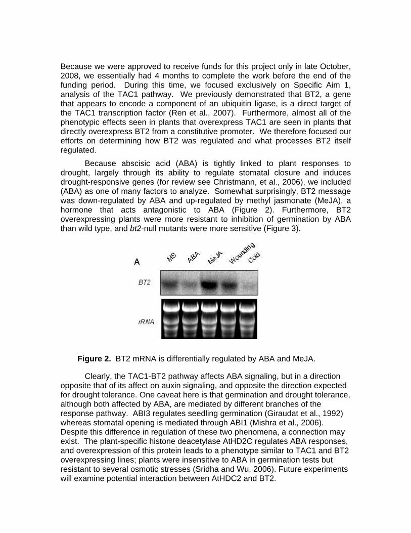
Because we were approved to receive funds for this project only in late October, 2008, we essentially had 4 months to complete the work before the end of the funding period. During this time, we focused exclusively on Specific Aim 1, analysis of the TAC1 pathway. We previously demonstrated that BT2, a gene that appears to encode a component of an ubiquitin ligase, is a direct target of the TAC1 transcription factor (Ren et al., 2007). Furthermore, almost all of the phenotypic effects seen in plants that overexpress TAC1 are seen in plants that directly overexpress BT2 from a constitutive promoter. We therefore focused our efforts on determining how BT2 was regulated and what processes BT2 itself regulated. Because abscisic acid (ABA) is tightly linked to plant responses to drought, largely through its ability to regulate stomatal closure and induces drought-responsive genes (for review see Christmann, et al., 2006), we included (ABA) as one of many factors to analyze. Somewhat surprisingly, BT2 message was down-regulated by ABA and up-regulated by methyl jasmonate (MeJA), a hormone that acts antagonistic to ABA (Figure 2). Furthermore, BT2 overexpressing plants were more resistant to inhibition of germination by ABA than wild type, and bt2-null mutants were more sensitive (Figure 3).

Clearly, the TAC1-BT2 pathway affects ABA signaling, but in a direction

opposite that of its affect on auxin signaling, and opposite the direction expected for drought tolerance. One caveat here is that germination and drought tolerance, although both affected by ABA, are mediated by different branches of the response pathway. ABI3 regulates seedling germination (Giraudat et al., 1992) whereas stomatal opening is mediated through ABI1 (Mishra et al., 2006). Despite this difference in regulation of these two phenomena, a connection may exist. The plant-specific histone deacetylase AtHD2C regulates ABA responses, and overexpression of this protein leads to a phenotype similar to TAC1 and BT2 overexpressing lines; plants were insensitive to ABA in germination tests but resistant to several osmotic stresses (Sridha and Wu, 2006). Future experiments will examine potential interaction between AtHDC2 and BT2.

Figure 2. BT2 mRNA is differentially regulated by ABA and MeJA.

Additional research revealed that BT2 expression is affected by multiple signals, including nutrients, biotic and abiotic stress (see cold lane in Fig. 2), and light. BT2 itself is required for proper response to many of these regulatory factors, suggesting that it acts as a major node in a pathway that integrates inputs from multiple and diverse signals, and coordinates appropriate responses to them. A manuscript describing this work is currently under revision for Plant Physiology (Mandadi, et al., 2009). We gratefully acknowledged the critical support provided by this grant. References Cited: Giraudat, J., Hauge, B.M., Valon, C., Smalle, J., Parcy, F., and Goodman, H.M. (1992) Isolation of the Arabidopsis ABI3 gene by positional cloning. Plant Cell. 4, 1251-1261. Mandadi, K.K., Misra, A., Ren, S., and McKnight, T.D. (2009) BT2, a BTB protein, mediates multiple responses to nutrients, stresses, and hormones in Arabidopsis thaliana. In revision for Plant Physiology. Mishra, G., Zhang, W., Deng, F., Zhao, J., Wang, X. (2006) A bifurcating pathway directs abscisic acid effects on stomatal closure and opening in Arabidopsis. Science 312, 264-266.

Figure 3. BT2 affects inhibition of germination by ABA. bt2 –null mutants (pink line) are more sensitive to effects of ABA on germination, whereas BT2 overexpressing plants (black line) are more resistant.

Ren, S., Johnston, J.S., Shippen, D.E., and McKnight, T.D. (2004) TELOMERASE ACTIVATOR1 induces telomerase activity and potentiates responses to auxin in Arabidopsis. Plant Cell, 16, 2910-2922. Ren, S., Mandadi, K.K., Boedeker, A.L., Rathore, K.S., and McKnight, T.D. (2007) Regulation of telomerase in Arabidopsis by BT2, an apparent target of the TELOMERASE ACTIVATOR1. Plant Cell, 19, 23-31. Sridha, S., and Wu, K. (2006) Identification of AtHD2C as a novel regulator of abscisic acid responses in Arabidopsis. Plant J. 46, 124-133.

Using SWAT to Compare Planning Methods forNeighborhoods: Case Study of Stormwater in TheWoodlands, Texas

Basic Information

Title: Using SWAT to Compare Planning Methods for Neighborhoods: Case Study ofStormwater in The Woodlands, Texas



District: 17

Research Category: Climate and Hydrologic ProcessesFocus Category: Floods, Management and Planning, Water Quality


Investigators: Bo Yang, Ming-Han Li

Publication

Yang, Bo, 2009. Assessing Planning Approaches by Watershed Streamflow Modeling: Case Study ofThe Woodlands, Texas, “Ph.D. Dissertation (paper 1),” Department of Landscape Architecture &Urban Planning, College of Architecture, Texas A&M University, College Station, Texas, 37 pages(dissertation paper 1).

1.

Yang, Bo, Ming-Han Li, 2008, Comparing Planning Methods for Neighborhoods: Case Study ofStormwater in The Woodlands, Texas, in book of abstracts of 49th Association of Collegiate Schoolsof Planning (ACSP) conference, Chicago, Illinois, page 521.http://www.acsp.org/events/2008_Conference_Archive.htm

2.

Yang, Bo, Ming-Han Li, 2009, Comparing Planning Methods for Neighborhoods: Case Study ofStormwater in The Woodlands, Texas, in book of abstracts of 2008-2009 Council of Educators inLandscape Architecture (CELA) conference, Tucson, Arizona, page 250.

3.

Using SWAT to Compare Planning Methods for Neighborhoods: Case Study of Stormwater in The Woodlands, Texas1

Page 1 of 12

Using SWAT to Compare Planning Methods for Neighborhoods: Case Study of Stormwater in

The Woodlands, Texas

2008-2009 USGS Research Grant Final Report For

Texas Water Resources Institute (TWRI) Project number: 06HQGR0130

Texas A&M University, College Station, Texas

May 18, 2009

Bo Yang, Ph.D. Candidate (PI) Dept. of Landscape Architecture & Urban Planning


Ming-Han Li, Ph.D., Assistant Professor (Co-PI) Dept. of Landscape Architecture & Urban Planning


Chang-Shan Huang, Ph.D., Associate Professor (Co-PI) Dept. of Landscape Architecture & Urban Planning


Page 2 of 12

ABSTRACT The Woodlands, Texas, has been well known as a town created with Ian McHarg’s ecological planning approach. Very few studies, however, have quantitatively measured the effect of this planning approach on stormwater management. In this study, two hypothetical land-use scenarios were created using different planning approaches: conventional low-density and cluster high-density. Both scenarios were compared with Ian McHarg’s approach using the Soil and Water Assessment Tool hydrologic model. The results suggest that Ian McHarg’s approach using soil permeability to coordinate development densities and land use is an effective planning strategy to mitigate environmental impacts from a stormwater perspective. KEYWORDS: GIS, Flood Mitigation, Soil Permeability, Urban Planning, Ecological Planning

Page 3 of 12

INTRODUCTION Considerable literature exists concerning urbanization-induced hydrological alterations (Paul

and Meyer, 2001). This is because urban development reduces infiltration capacity of the natural landscape and increases stormwater flows. In community development, conventional practice imposes a homogenous hardscape pattern on the natural landscape, giving little consideration to advantageous drainage opportunities. Drainage designs often aim to remove stormwater as quickly as possible, thus providing a flooding problem downstream (Booth and Jackson, 1997).

A built example of an infiltration-based planned community is The Woodlands, Texas. It is the first master-planned community that employed an ecological approach in the 1970s. The planning concept was to determine building densities and land use based on the hydrologic properties of the soil. This was done by preserving land with high soil permeability as open space and using land with low soil permeability for commercial or residential developments (McHarg and Sutton, 1975; McHarg, 1996). Despite the lack of rigorous scientific evaluations, this ecological planning approach is regarded as successful based on extreme storm events. The Woodlands survived the one-hundred-year storms in 1979 and 1994 with little property damage, while Houston, 31 miles away, was severely flooded in both events (Girling and Kellett, 2005).

This study aimed at answering two questions: (1) whether or not The Woodlands development adhered to McHarg’s original plans overtime, and (2) which community planning approach (conventional low-density, cluster high-density, and The Woodlands approaches) causes less development impacts in terms of stormwater runoff. We created two “what if” land-use scenarios for The Woodlands: a conventional low-density plan, ubiquitous in the U.S. (e.g., Houston), and a cluster high-density plan which leaves a large amount of open space for stormwater detention and infiltration (Center for Watershed Protection, 1994). Moreover, we prepared a third homogeneous forest land-use scenario as the baseline condition to stand for The Woodlands prior to any development (Soil Conservation Service, 1972). These different scenarios were compared by simulating stormwater runoff in the Soil and Water Assessment Tool (SWAT). Finally, development densities and locations led by different planning approaches were discussed and compared with previous studies. STUDY SITE AND METHODS

The study area is the Panther Creek watershed, where The Woodlands is located (Figure 1). The majority of The Woodlands is within this watershed, and is a sub-watershed of the Spring Creek watershed, USGS Hydrologic Unit Code 12040102. Interstate Highway 45 runs to the east of The Woodlands, and is a major transportation corridor connecting Houston (30 miles away) to the south and Dallas/Fort Worth (210 miles away) to the north. The drainage area of the Panther Creek watershed is 36.4 square miles (23,266 acres).

Page 4 of 12

Figure 1. Panther Creek watershed development and stream network. Residential development densities are categorized by fraction total impervious area (FIMP): (1) residential low density, FIMP=0.12, (2) residential medium density, FIMP=0.38, and (3) residential high density, FIMP=0.6 (USGS).

Page 5 of 12

Data We obtained historical weather data (1970-2007) from the National Climate Data Center

(NCDC) website (NCDC). We downloaded river reach files of the watershed from the National Hydrograph Dataset website (NHD), and topographical data from the USGS National Map Seamless Data Distribution System (USGS). From various national land-use datasets, we downloaded land-use and land-cover information for four years (1984, 1996, 2001 and 2005). The soil data we used was the high-resolution Soil Survey Geographic (SSURGO) dataset developed by the Natural Resources Conservation Service (NRCS). Land-use Change and Development Location

The first set of analyses evaluated whether or not The Woodlands development followed McHarg’s ecological plans over a 35-year period. The question to be examined was: “Did The Woodlands preserve more permeable soils than impermeable soils in the community development?” We examined the land-use and land-cover change in the watershed of four years (1984, 1996, 2001, and 2005). Furthermore, we overlaid land-use and land-cover grids with soil grids to quantify the percentages of impervious cover on each soil group. Soils in the watershed were grouped according to their hydrologic properties defined by U.S. Department of Agriculture (USDA, 2002). There are four hydrologic soil groups. A soil stands for sandy and loamy sand soils, which allow the highest infiltration. D soil represents clay loam and clay soils that are almost impermeable. B and C soils are in between (Table 1).

Table 1. Hydrologic soil groups (USDA, 2002) Hydrologic soil group Soil texture Saturated infiltration rate

(mm/hr) A Sand and loamy sand 50-200 B Sandy loam and loam 12.7-25 C Silt loam and sandy clay loam 3.8-6.3 D Clay loam, silty clay loam and clay 1.3-2.3 Planning Approaches and Land-use Scenarios

The second set of analyses assessed whether or not The Woodlands development was superior to those engendered by other planning approaches. The question to be examined was: “Will there be greater impacts if the residential land-uses changed their densities and locations according to other planning approaches?” Hypothetical scenarios were created to provide optimum or worst conditions which either solely based on, or contrary to McHarg’s planning approach. That is, when impervious cover is added onto impermeable soils, the least impacts on the watershed will be engendered. More profound impacts are expected if more permeable soils are paved over.

We used The Woodlands 2005 land-use conditions to define the impervious cover area in the watershed and created two scenarios which maintained the same imperviousness. Since impervious cover continues to be the single most important variable affecting watershed runoff,

Page 6 of 12

it is important to hold this variable constant so that scenarios would be comparable. Urban developed area, primarily residential land-uses, was used as a substitute for impervious cover. According to the USGS, there are three residential land-use densities and each has a range of impervious cover percentage. We created an impervious cover ratio index to control the total impervious area. This ratio index made it possible to change from one density to another, and from one approach (e.g., low-density) to another (e.g., high-density).

The procedure was described in Table 2. Firstly, we assigned the lowest median value (that of the low-density) a ratio of one. Secondly, we calculated the ratios for two other densities based on their median values. For example, it will require 2.6 acres low-density residential land to match the same impervious area of one-acre high-density residential land. Finally, all urban land-uses were changed to high-density residential land in Scenario 1, and to low-density residential land in Scenario 2.

Table 2. Impervious cover ratio index Land Use Impervious % Median Ratio Residential low density 20-49 35 1.0 (baseline) Residential medium density 30-79 55 1.6 Residential high density 80-100 90 2.6 Commercial/industrial/transportation 80-100 90 2.6

We referred to the general trend of The Woodlands development in history and also considered the soil patches when we allocated development in the watershed (Figure 2). The first village started at downstream of the Panther Creek, and development evolved along the creek to the north. Detailed procedure was explained in Table 3. This procedure minimized the possibility of assigning development randomly in the watershed. Model and Measurement

We used the Soil and Water Assessment Tool (SWAT) to simulate scenarios. SWAT, embedded in ArcGIS interfaces, is a hydrologic and water quality model widely used in agriculture dominated land uses (Srinivasan and Arnold, 1994). An increasing number of studies have demonstrated its capabilities for urban watershed modeling (Fohrer et al., 2000). In the SWAT model, each unique combination of land-use and soil-type will generate a unique Hydrologic Response Unit (HRU). Therefore, superimposing varying land-use types onto different soil patches will generate runoff quantities for comparison. In the SWAT model, each HRU is directly related to a curve number (CN) (Srinivasan and Arnold, 1994). The CN method was developed by the NRCS, and is an infiltration and runoff model widely used among engineers and watershed managers. The composite CNs were calculated for the watershed for seven land-use scenarios and conditions. Finally, watershed outputs (runoff and sediments) were simulated using SWAT.

Page 7 of 12

Figure 2. Land-use scenarios 1-3 and watershed soil conditions A-D.

Page 8 of 12

Table 3. Land-use scenarios and observed land-use conditions in the Panther Creek watershed Hypothetical Scenarios

Land-use condition % Urban Watershed CN

Data1

1 (high-density) Optimal condition. High-density development takes place on C and D soils. In the meantime, the general trend of development from downstream to upstream was maintained.

49% 73.3 HGAC

2 (low-density) Worst condition. Low-density development takes place on A and B soils.

49% 80.8 HGAC

3 (baseline) Forest-dominated condition. Developed lands (e.g., residential and commercial) were changed to evergreen forest, while other natural land-covers were maintained (e.g., wetland, herbaceous, etc.)

0% 66.9 HGAC

Observed Conditions

1984 26% 71.6 EPA 1996 37% 72.1 NLCD 2001 48% 77.6 HGAC2005

Mixed condition. Development takes place on both A/B soils and C/D soils, and densities of development comprise of low, medium and high densities. 49% 80.4 HGAC

1. The land-use and land-cover datasets are 1984 EPA GIRAS data (1:250,000 scale), 1996 National Land Cover Dataset (NLCD) (1:24,000 scale), and 2001 and 2005 Houston Galveston Area Council (HGAC) costal data (1:24,000 scale). RESULTS Land-use Change and Development Location

The Panther Creek watershed (The Woodlands) experienced rapid urban development since its beginning in the 1970s (Figure 3). The forest-dominated natural landscapes shifted to residential-dominated land-uses, which occupied nearly half of the watershed by 2005. There are 22 land-use and land-cover categories in the USGS datasets. We further collapsed them into seven categories: (1) water (open water, woody wetlands and emergent herbaceous wetlands), (2) urban (low density residential, medium density residential, high density residential, and commercial/industrial/ transportation), (3) forest (deciduous forest, evergreen forest, and mixed forest), (4) agriculture (pasture/hay, row crops, and small grains), (5) grassland, (6) grasslands/herbaceous, shrubland, urban/recreational grasses, and (7) others (bare rock/sand/clay and transitional).

Page 9 of 12

Figure 3. Land-use and land-cover change in the Panther Creek watershed (The Woodlands)

There were smaller percentages of permeable soils (A and B soils) available than

impermeable soils (C and D soils) in the watershed (Table 4). Keeping these permeable soil patches intact as open space was essential for stormwater infiltration and flood mitigation. Unexpectedly, for each of the four years examined, more development took place on A and B soils compared to C and D soils. Table 4. Development location on different soil groups in the Panther Creek watershed

Hydrologic Soil Group A B C D

Total area (acre) 1265 2130 1146 2322 Develop on soil Acre % Acre % Acre % Acre % 1984 463 37% 707 33% 123 11% 463 20% 1996 512 40% 861 40% 281 25% 898 39% 2001 585 46% 1276 60% 489 43% 1056 45% 2005 585 46% 1276 60% 525 46% 1059 46% Scenario Simulation and CN Modeling

As we expected, the cluster high-density scenario (Scenario 1) generated the least amount of runoff and sediments, while the low-density scenario (Scenario 2) generated the most for both (Figure 4). However, the Woodlands 2005 status quo condition generated marginally lower outputs than the low-density scenario, which was the worst scenario in this study. This result was in accordance with the 2005 observed land-use conditions in which watershed CN reached 80.4,

0

2500

5000

7500

10000

12500

15000

17500

20000

Water Urban Forest Agriculture Grassland Other

Are

a (a

cre)

1984 1996 2001 2005

Page 10 of 12

slightly lower than 80.8 in the low-density scenario. It is noteworthy that all scenarios caused higher watershed outputs than the forest baseline scenario (Scenario 3). It is also important to note that values in Figure 4 are averaged values for the entire watershed. If multiplied by the watershed area (23,266 acres), the low-density scenario generated 17,482 acre-feet stormwater runoff and 292 tons sediments more than that of the forest scenario on a yearly basis. Figure 4. Simulated surface runoff and sediment yields of four land-use scenarios. DISCUSSION

Our results suggest that The Woodlands land-use conditions worsened in comparison with what the original McHarg plans proposed. Soils with sound infiltration capacities were not given first priority in the community plans. A significant setback from the original plans took place in 1985 although the spirit of the “Ecological Plan” remained in the community mission statement (Girling and Helphand, 2003). The year 1997 witnessed a further adjustment to the plans when George Mitchell sold The Woodlands ownership to Crescent Real Estate Equities and Morgan Stanley Real Estate Fund II, after which even more intensive development occurred (Clay, 1998). Despite these negative deviations, a green infrastructure was established and maintained relatively well in the following years. This green infrastructure includes maintenance of 100-year flood plains of the three creeks on site, drainage easements, greenways, and more than 100 parks (108 by year 2007). In sum, 25% of the land will ultimately be preserved as open space (Galatas and Barlow, 2004).

The simulation results are consistent with the previous studies on the relationship of

0.0

50.0

100.0

150.0

200.0

250.0

300.0

350.0

400.0

450.0

500.0

Forest High density 2005 Status quo Low density

Suf

ace

Run

off (

mm

)

0.0000

0.0100

0.0200

0.0300

0.0400

0.0500

0.0600

0.0700

0.0800

Sed

imen

t (To

n/ha

)

Surface Runoff (mm) Sediment (Ton/ha)

Page 11 of 12

development densities and watershed outputs (Schueler, 1994; Stone, 2004). Our results further demonstrate that when total impervious cover is held constant, the high-density compact development generated around 30% less runoff compared to the low-density development. Compared with the forest condition, both Scenarios 1 and 2 increased runoff. The high-density development increased runoff around 43%, and less than half of 94% caused by the low-density development. As a result, we echo McHarg’s ecological planning approach and suggest that the location of development, particularly, on top of which type of soils, is an important factor. CONCLUSION

Our results suggest soils with high infiltration capacities were not given first priority in land preservation in The Woodlands. This result may be because the data we used made it impossible to replicate the process conducted by McHarg and his colleagues. Land-use and land-cover, topography, and soil datasets we used are at resolutions of 30m x 30m or 80m x 80m. However, intensive soil survey, vegetation inventory, and site topography analysis were conducted in the 1970s (McHarg and Sutton, 1975). Therefore, detailed drainage designs at site level could not be reflected by the coarse datasets we used. In addition, the inconsistency between land-use and land-cover data provided by different agencies may contribute to the artifact in our results.

The challenge of balancing development and land preservation is universal. Development in a watershed encourages flooding. The Woodlands current conditions, though of less quality than originally proposed, are further ahead in promoting a sustainable community development model than conventional solutions (Forsyth, 2002). Even though environmental data, particularly soil data, may cease to be used to determine which location and what proportion of the land is to be developed, The Woodlands’ planning, design, and management presents an excellent example of eco-conscious community planning for the design professionals to consider. ACKNOWLEDGEMENTS The study is funded by the Texas Water Resource Institute (TWRI) through the USGS 104B program (Project number: 06HQGR0130). The authors express their gratitude to Debra Staley and Mike Mooney for gracious help on research data and coordination. Special credit must also go to Steven Johnson for valuable suggestions and sharing first-hand information of planning and design of The Woodlands. REFERENCES Booth, D.B., Jackson, C.R. 1997. Urbanization of Aquatic Systems: Degradation Thresholds,

Stormwater Detention, and the Limits of Mitigation. Journal of the American Water Resource Association, 22, 1-19.

Center for Watershed Protection, 1994. Use of Cluster Development to Protect Watersheds.

Page 12 of 12

Watershed Protection Techniques, 1, 137-140. Clay, G. 1998. The National Observer: The Woodlands. Landscape Architecture, 88 (9), 131-132. Fohrer, N., Haverkamp, S., Eckhardt, K., Frede, H., 2000. Policy induced land use changes and

their effects on land degradation: A modeling approach. Congress of ESSC. Valencia 28, 3-14.

Forsyth, A. 2002. Planning Lessons from Three U.S. New Towns of the 1960s and 1970s: Irvine, Columbia, and The Woodlands. Journal of American Planning Association, 68, 387-415.

Galatas, R., Barlow, J. 2004. The Woodlands: The Inside Story of Creating a Better Hometown. Washington D.C.: The Urban Land Institute Press.

Girling C., Kellett, R. 2005. Skinny streets and green neighborhoods: design for environment and community. Washington, D.C.: Island Press.

Girling, C.L., Helphand, K.I., 1994, Yard, Street, Park: The Design of Suburban Open Space. New York: John Wiley and Sons.

McHarg, I.L. 1996. A Quest for life: an autobiography. New York: John Wiley and Sons. McHarg, I.L., Sutton, J. 1975. Ecological Plumbing for the Texas Coastal Plain. Landscape

Architecture, 65 (1), 80-89. National Climatic Data Center (NCDC). Available from http://www.ncdc.noaa.gov/oa/ncdc.html National Hydrograph Dataset (NHD). Available from http://nhd.usgs.gov Natural Resources Conservation Service. Soil Survey Geographic (SSURGO) Database.

Available from http://soils.usda.gov/survey/geography/ssurgo/ Paul, M.J., Meyer, J.L. 2001. Streams in the urban landscape. Annu. Rev. Ecol. Syst., 32, 333-

365. Schueler, T. 1994. The Importance of Imperviousness. Watershed Protection Techniques, 1,

100-111. Soil Conservation Service, 1972. Soil survey of Montgomery County, Texas. Washington, D.C.:

U.S. Government Printing Office. Srinivasan, R., Arnold, J. 1994. Integration of a Basin-Scale Water Quality Model with GIS.

Water Resources Bulletin, 30, 453-462. Stone, B. 2004. Paving over paradise: how land use regulations promote residential

imperviousness. Landscape and Urban Planning, 69, 101-113. U.S. Department of Agriculture, Natural Resources Conservation Service. 2002. National Soil

Survey Handbook, title 430-VI. U.S. Geological Survey. National land cover dataset 2001 (NLCD). Available from

http://seamless.usgs.gov/website/seamless/products/nlcd01.asp

An Environmental Flows Information System for Texas

Basic Information

Title: An Environmental Flows Information System for TexasProject Number: 2008TX311B


Funding Source: 104BCongressional District: 21

Research Category: Climate and Hydrologic ProcessesFocus Category: Ecology, Hydrology, Surface Water

Descriptors: NonePrincipal Investigators: Eric S Hersh, David R. Maidment

Publication

Hersh, E.S. and D.R. Maidment, September 2008, “Managing Information for Environmental Flowsin Texas” in Environmental Information Management Conference, Albuquerque, New Mexico.

1.

Hersh, E.S., D.R. Maidment, and W. Gordon, October 2008, “An Environmental Flows InformationSystem for Texas” in Texas GIS Forum, Austin, Texas.

2.

Hersh, E.S. and D.R. Maidment, October 2008, “An Environmental Flows Information System forTexas” in Instream Flow Council FLOW2008, San Antonio, Texas.

3.

Hersh, E.S. October 2008, “A Texan’s Perspective on Environmental Flows” U.S. Geological Survey,Northborough, Massachusetts.

4.

An Environmental Flows Information System for Texas 1

FINAL REPORT: An Environmental Flows Information System for Texas

Project Number 570463

Principal Researcher (graduate student): Eric S. Hersh Principal Investigator (faculty advisor): David R. Maidment

Abstract Data describing the stream flow, water chemistry, geomorphology, and biology of streams and rivers is often contained in a variety of formats and in many geographic locations. We have developed an information system to facilitate the discovery, acquisition, and sharing of data relevant to the study of environmental flows, including data from hydrology and hydraulics, water quality, climatology, geomorphology and physical processes, and biology. Working cooperatively with the Consortium of Universities for the Advancement of Hydrologic Science, Inc. (CUAHSI) Hydrologic Information System (HIS) project, an NSF‐supported effort to improve access to hydrologic data at the nation’s universities, environmental flows data are stored in the CUAHSI Observations Data Model and web services are established for the computer‐to‐computer communication of data in order to extract data from disparate sources in disparate formats, to transform the data into the common language of CUAHSI WaterML, and to load the data into an end user’s system. The environmental flows information system includes a linkage to a georeferenced digital archive of documents, providing for parallel access to both data and the knowledge products derived from that data. Via the Data Model and accompanying Document Model, an information system capable of managing observational data, geographic data, modeled/constructed data, and documents is offered. A prototype environmental flows information system is developed for the State of Texas that incorporates relevant known available datasets from federal, state, academic, river basin, and local sources. Tools are developed to assist in the publishing, visualization, and access of data and documents via map‐based, spreadsheet‐based, and other methods. The information system might be used to provide: (1) rapid low‐cost data integration, (2) improved data access by the public, and (3) support for the analysis and determination of environmental flow needs. The environmental flows information system represents the integration of the physical, chemical, and biological information for rivers and streams in a consistent and accessible manner in one system in one place.

Problem and Research Objectives

Environmental flow or instream flow is the water left in or released into a river system, often for

managing some aspect of its conditions. The goal may be, for example, the broad maintenance of a

healthy river ecosystem or the narrow focus of ensuring the survival of an individual. But freshwater is a

finite and essential resource, and humans have exploited this resource with great success for many

millennia: agriculture, industry, recreation, hydropower, and we continue to do so in an accelerating

fashion. What amount of freshwater can be withdrawn without impacting the riverine ecosystem? Is

there spare water in a river? How do you preserve the ecological integrity of a river system? And what

are the environmental impacts of using increasingly more water? While the concept of environmental

flows is simple and the need for environmental flow prescriptions seems intuitive to the enlightened

scientist, quantifying environmental flow needs effectively and efficiently remains a puzzle yet to be

solved.

In Texas, the Texas Commission on Environmental Quality (TCEQ) is tasked with developing instream

flow recommendations. However, no comprehensive database of information is available for review

and there is no systematic method for identifying or classifying Texas streams in order to determine the

applicability of existing methods. Moreover, the recently‐passed Senate Bill 3 tasks stakeholders and

regulators with determining and reviewing environmental flow needs, yet no comprehensive repository

of relevant data exists that could shared with these stakeholders as they embark on the tasks of

reviewing existing data and developing technical recommendations. Data describing the streamflow,

water chemistry, geomorphology, habitat, and biology of Texas streams and rivers is contained in a

variety of formats and in many geographic locations.

Thus, we seek to develop a data model and information system to store and make available

environmental flow data in a consistent and accessible format. The synthesis and integration of all

these data, in combination with GIS tools, will produce an Environmental Flows Information System that

will help TCEQ in establishing flow requirements in a systematic way across Texas. As such, the

objectives of this project are: (1) create a comprehensive Environmental Flows Information System Data

Model that would provide the format and organizing scheme for different data layers (hydrology &

hydraulics, water quality, climatology, geomorphology & physical processes, and biology); (2) perform

case studies to show how the attributes of this system can be used to support environmental flow

determinations at selected sites in the state; and (3) deliver a database and toolset which will enable

the TCEQ to operate the Environmental Flows Information System at the conclusion of the project.

Accomplishments, March 1, 2008 through February 28, 2009

In support of environmental flow efforts ongoing in the State of Texas, a data model has been created

which brings together geospatial, physical, chemical, and biological data along with supporting

documents and base maps. Collectively, these items form an “Environmental Flows Information

System.” Disparate data sources have been identified, acquired, and ingested, and a website has been

created to serve as a repository for these data (http://data.crwr.utexas.edu/). The website includes

dozens of Texas water data services (i.e., web‐enabled datasets) stored in one of five common formats.

Major data contributors include the three primary water agencies: the Texas Commission on

Environmental Quality, the Texas Water Development Board, and the Texas Parks and Wildlife

Department, along with other federal, state, local, and academic data providers. Included in the data

inventory is information specifically related to the instream flow studies already conducted on the

Sabine and San Antonio Rivers.

Working with the Texas Natural Resources Information System, the State’s digital data agency, a web‐

based map viewer has been created (http://www.waterdatafortexas.org/) to allow the public access to

discover and access data relevant to their interests and needs. The thematic organization has been

provided to TNRIS, as has guidance on the user interface/ user experience, data access, content, and

testing. Tools for improved data download and data analysis are currently being installed and tested. In

addition, a thematic‐based framework for data discovery has been developed whereby a user can simply

opt to search for data related to a concept of interest (such as “salinity” or “water temperature” or

“fish”) rather than to sift through the data from individual data providers.

In addition to data, access to existing documents is a valuable and necessary tool for future scientific

and engineering analyses. Some documentation is readily available through various means. Much is

currently unavailable, however: a significant detriment to accomplishing the goal of establishing

environmental flow needs. A project was undertaken to organize and foster access to documents,

reports, and studies. For this demonstration project, the river basin and bay system consisting of the

Trinity and San Jacinto Rivers and Galveston Bay formed the study area. In conjunction with the

University of Texas Libraries, the DSpace digital repository system was used to capture, store, index,

preserve, and redistribute documents

(https://repositories.lib.utexas.edu/handle/2152/4029/browse?type=title).

Finally, improved access to increasing data resources allows for improved analysis and increasing data

synthesis opportunities. Numerous hydrologic‐based desktop methods exist for environmental flows

but tools which link hydrology, hydraulics, and habitat are thus far lacking, leading to a dearth of

biologic‐based desktop methods. The availability of sufficient suitable habitat is critical to ensuring a

sound ecological environment. Traditional habitat assessments have consisted of detailed site‐specific

field work coupled with intensive hydrodynamic modeling efforts, and, while this state‐of‐the‐practice

methodology is ideal for certain situations, it can be prohibitively resource‐intensive for others. Drawing

upon a growing amount of digitally available information for aquatic biology, a desktop methodology,

termed BioDesktop, is being developed which seeks to establish the important flow‐habitat linkage and

to evaluate environmental flow needs.

Future Work

Upcoming project goals include refinement of the BioDesktop approach, the development of additional

analytic tools for the Environmental Flows Information System, the ingestion of additional biologic data

for Texas, the continued pursuit of an improved means for organizing and storing collections‐based

information (such as that commonly collected during biological studies, and as opposed to time‐series

based information), and continued documentation, workshops, meetings, and presentations to share

the results of these efforts.

Microbial Source Tracking in Drinking Water from RainwaterHarvesting

Basic Information

Title: Microbial Source Tracking in Drinking Water from Rainwater HarvestingProject Number: 2008TX312B



Research Category: Water QualityFocus Category: Conservation, Non Point Pollution, Water Quality

Descriptors: NonePrincipal Investigators: Brigit Afshar, Mary Jo Kirisits

Publication

Afshar, Brigit; Mary Jo Kirisits, Kerry Kinney, Carolina; 2009, Microbial Source Tracking inDrinking Water from Rainwater Harvesting, Texas Water Research Institute, United StatesGeological Survey, Texas.

1.

Microbial Source Tracking in Drinking Water from Rainwater Harvesting 1

Brigit Roeya Afshar | Abstract C-1

USGS Program Report Project Number: 2008TX312B The Effect of Roofing Material on Water Quality for Rainwater Harvesting Applications – A Field Study of Residential Roofs Primary PI: Brigit Roeya Afshar, EIT Other PIs: Dr. Mary Jo Kirisits and Dr. Kerry Kinney

May 2009

Abstract The pressing need for sustainable freshwater supplies has increased the use of roof-based

rainwater collection systems for potable and non-potable applications. Aside from the usual environmental factors that affect freshwater quality, such as seasons and location, roof-based rainwater collection systems also have synthetic components, including the roof catchment, that can contaminate the rainwater. The purpose of this study was to assess the effect of roofing material on the chemical and biological quality of rooftop-harvested rainwater. In this study, three existing residential roofs, one metal and two asphalt fiberglass shingle, were equipped with rainwater sampling devices to collect the roof runoff from multiple rain events during a single winter season. In addition, each site was equipped with an ambient sampler that collected rainfall that had not contacted the roof. The rainfall samples were tested for pH, conductivity, turbidity, and the concentrations of total solids, fecal and total coliform, nitrate (NO3

-), nitrite (NO2

-), total organic carbon (TOC), dissolved organic carbon (DOC), selected synthetic organic compounds, and selected metals. Microbial communities present in the ambient and harvested rainwater also were examined by performing a microbial community fingerprinting analysis called Terminal Restriction Fragment Length Polymorphism (T-RFLP). By holding other factors such as season, roofing area, and geographic region constant, this study inferred the influences of two different roofing material types on the quality of rooftop harvested rainwater.

Based on our chemical analyses, neither roofing material was determined to be superior to the other for rainwater harvesting. All harvested rainwater samples were within the expected pH range (pH 5-7). For all rain events, the conductivity, turbidity, and concentrations of total solids, total and fecal coliform, nitrate, nitrite, TOC, and DOC decreased as a function of roof flushing through the rain event. Our data show that the conductivity and concentrations of total coliform and fecal coliform from the metal roof were usually lower than those from the shingle roofs. However, turbidity and the concentrations of lead and zinc from the metal roof were usually higher than those from the shingle roofs. In addition, the data show that the total solids and concentrations of nitrate, nitrite, TOC, and DOC from the metal roof were intermediate of the concentrations from the two shingle roofs during at least one rain event, indicating that the quality of rooftop-harvested rainwater is not determined solely by roofing material. Although there are no regulations on private rainwater harvesting systems, we compared our data to potable water standards. Turbidity readings for every sample exceeded United States Environmental Protection Agency (EPA) regulations for filtered surface water systems, which means that filtration would be recommended if the harvested rainwater were to be used for potable purposes. The EPA states that no more than 5% of drinking water samples can test

Brigit Roeya Afshar | Abstract C-2

positive for coliform; however, all harvested rainwater samples for both roofing materials always contained detectable total and fecal coliform, indicating that treatment would be needed prior to potable use. Each harvested rainwater sample was less than the EPA’s maximum contaminant limit (MCL) for nitrate (10 mg/L NO3

--N) and nitrite (1 mg/L NO2--N), indicating that no

treatment for nitrate or nitrite would be necessary prior to potable use. The zinc concentrations in the harvested rainwater were significantly lower than the EPA secondary guidelines of 5000 µg/L, meaning that no additional treatment would be needed for zinc removal prior to potable use. In addition, since none of the harvested rainwater samples contained greater than the EPA action level of 15 µg/L for lead, no additional treatment would be needed for lead removal prior to potable use. The harvested rainwater samples were tested for a suite of 200 synthetic organic compounds on the first flush samples from one rain event for the metal roof and one of the shingle roofs. Only two compounds were detected: benzyl alcohol and 2,4-dinitrophenol; the concentrations were very low, and both compounds are unregulated in drinking water.

Data from several parameters, such as conductivity, nitrate, TOC, and DOC, show decreasing water quality as a function of the number of dry days prior to the rain event. The data also suggest that the amount of overlying vegetation can impact water quality. The data clearly indicate the benefit of using a first flush diverter to divert the initial (and most contaminated) portion of the rainwater from the storage tank.

We examined the microbial diversity of ambient rainwater and harvested rainwater using T-RFLP. The metal roof showed reduced microbial community diversity as compared to the shingle roofs. Although the microbial diversity from the metal roof was greatly reduced as compared that from the shingle roofs, it is not known which roofing type supported greater numbers or more types of pathogens. Microbial diversity also decreased with roof flushing on the metal roof. Our analysis showed greater microbial diversity in the first flush harvested rainwater as compared to ambient rainwater, demonstrating that additional microorganisms are being collected from the roof surface. Despite the fact that the two shingle roofs tested are 20 miles apart, they displayed similar T-RFLP profiles.

This study examined harvested rainwater quality from metal and shingle roofs over a winter season in Texas. Neither metal nor shingle roofing materials were clearly superior to the other in terms of overall harvested rainwater quality. Although the data set was limited, several conclusions can be made from the data collected. First, the quality of the rooftop-harvested rainwater increased with roof flushing as the rain event progressed, indicating the importance of an effective first-flush diverter; these findings are consistent with previous studies. Second, the quality of the rooftop-harvested rainwater varied even when holding the roofing material constant, illustrating that quality is a function of several other factors. Even within the same rain event and across the same type of roofing material and roof age, the harvested rainwater quality also might be affected by roof dimensions, amount of overlying vegetation, and level of wildlife activity on the roof. Third, this study found several constituents in the harvested rainwater to be above the maximum recommended levels for drinking water, suggesting the need for treatment regulations to be implemented if the harvested rainwater is intended for potable use. With rainwater emerging as a renewable alternative to diminishing traditional freshwater sources, it is critical to have a comprehensive understanding of the quality of harvested rainwater as affected by roofing materials.

Ecohydrology and ecophysiology of Arundo donax (giantreed)

Basic Information

Title: Ecohydrology and ecophysiology of Arundo donax (giant reed)Project Number: 2008TX314B


Funding Source: 104BCongressional District: 15, 27, 28

Research Category: Biological SciencesFocus Category: Acid Deposition, Non Point Pollution, Water Quantity

Descriptors:Principal Investigators: David Watts, Georgianne Moore

Publication

Watts, David A., 2009, Dynamics of water use and responses to herbivory in the invasive reed,Arundo donax (L.), "MS Thesis," Ecosystem Science and Management, College of Agriculture andLife Sciences, Texas A&M University, College Station, Texas, 77 pp.

1.

Ecohydrology and ecophysiology of Arundo donax (giant reed) 1

REPORT

Title Ecohydrology and ecophysiology of Arundo donax (giant reed) Project Number 2008TX314B (40770) Primary PI David Watts (former graduate student) Ecosystem Science & Management Texas A&M University 123 Animal Industries Building 2138 TAMU College Station, TX 77843 [email protected] Other PIs Dr. Georgianne Moore (faculty advisor) Ecosystem Science & Management Texas A&M University 325 Animal Industries Building 2138 TAMU College Station, TX 77843 [email protected] 979-845-3765 Abstract The primary objective of this research was the investigation of the impact of the invasive grass species, Arundo donax L. (giant reed), on the water cycle. At a site on the Rio Grande in South Texas, we measured the gas exchange of carbon dioxide and water vapor on leaves of A. donax. At the stand scale, we measured structural characteristics, such as leaf area and shoot density. Data were collected along transects of two types, one for each of the leaf scale and stand scale measurements made. We constructed a model to estimate stand scale estimation by multiplying leaf level measurements by data for stand level structural properties in order to estimate the quantity of water used in mm per day. At this site, A. donax used roughly 9 mm of water per day, which is at the high end of the spectrum for most plants. This value is averaged from measurements during two summer seasons and the winter between. We determined that the major controls on stand scale transpiration were evaporative demand, leaf area index, and water availability. Stand transpiration varied greatly but tended to be highest in measurements made following precipitation events, which suggests that A. donax may use soil moisture derived from precipitation rather than groundwater. Problem and Research Objectives

Arid and semi-arid regions are inherently water-limited, and there are important

relationships between the biological and hydrological aspects of these landscapes (Wilcox and Newman 2005, Newman et al. 2006). Recent studies in ecohydrology have focused attention on two primary interacting components – the riparian corridors and the upland rangeland areas. Of particular focus in the study of semi-arid rangelands are causes and effects of the protracted expansion of woody plants (Archer 1989, Schlesinger et al. 1990, Archer 1994, Ansley et al. 1995, Van Auken 2000, Archer et al. 2001, Huxman et al. 2005, Potts et al. 2006). Within riparian zones, ecohydrological research has concentrated on the role of woody plants generally, and especially invasive species like Tamarix spp., frequently seeking to assess whether these plants are causes and/or effects of changes in the hydrologic regimes of watersheds (Busch et al. 1992, Sala et al. 1996, Stromberg 1998, Scott et al. 2000, Tabacchi et al. 2000, Stromberg 2001, Cleverly et al. 2002, Dahm et al. 2002, Nagler et al. 2003, Glenn and Nagler 2005, Stromberg et al. 2007, Moore et al. 2008, Nagler et al. 2008a, Nagler et al. 2008b).

Little is known about the interactions between non-woody species and the water cycle in these semi-arid riparian zones, in spite of the fact that they are known to also affect riparian ecosystems (Naiman and Decamps 1997). Arundo donax has previously been labeled a ‘transformer’ species (Spencer et al. 2005) because it has been shown to negatively impact both biodiversity (Herrera and Dudley 2003, Kisner 2004, Guthrie 2007) and ecosystem function (Rieger and Kreager 1989, Scott 1994, Quinn et al. 2007, Quinn and Holt 2008). However, the impact of A. donax on water resources has not yet been quantified. Because this species already covers large amounts of land in the already stretched Rio Grande watershed, basic information on rates of water use at multiple spatial and temporal scales are needed to begin to understand how A. donax functions in contemporary ecosystems. Materials/Methodology

A research site was established within a large monoculture of Arundo donax along the Rio Grande near the town of Los Indios, TX. Here three transects, each between 12 and 20 m in length, were established perpendicular to the Rio Grande in order to investigate leaf scale physiological processes. Each transect contained four 1 m by 1 m plots that were evenly spaced relative to the total length of the transect. Each plot consisted of four leaves on which measurements of carbon dioxide and water vapor exchange were made. These gas exchange measurements were conducted with a LI-6400 open-pathway system. Carbon dioxide and photosynthetically active radiation were controlled using a CO2 injector and LED light source, respectively. Measurements of leaf gas exchange were conducted on 23 days between 27 June, 2007 and 22 July, 2008.

In order to quantify metrics of stand structure and document patterns in phenological development, ten additional transects were destructively sampled at approximately two month intervals between July 2007 and March 2008. As above, transects were divided into four 1.0 m2 plots, each of which was further subdivided into three vertical sections based on the maximum height of the canopy in the stand of A. donax. Density of all shoots and diameter and height of each shoot was measured in each of the plots. In 0.25 m2 subplots, total leaf area was quantified using a leaf area meter for five of the ten transect in order to derive estimates of leaf area index (area of leaf cover per unit area of ground).

The purpose of this study design was to assess the effect of water available to plants within the stand along a potential moisture gradient, with plant available water expected to decrease with increasing distance from the river’s edge. The existence of this moisture gradient was tested through the use of stable carbon isotope ratios (δ13C) (Farquhar et al. 1989, Ehleringer et al. 1993, Dawson et al. 2002). Leaves used for gas exchange were collected, dried until they reached a constant mass, and ground for isotope analysis. Principal Findings The Arundo donax stand we studied is notably productive for a graminoid species, for the mean leaf area index in our study site exceeded 4 m2 per m2, which is a high value for a non-cultivated grass. Our value is greater than those found in stands of Tamarix ramosissima in a different part of the same watershed (Dahm et al. 2002). The value of leaf area index ranged from 3.3 to 5.5, although this range did not indicate a seasonal trend, but rather a relatively constant rate of growth that ended with a leaf abscission event that occurred at some time between two sampling periods. Leaf area index also was highest in the plots closest to the river. Similarly, rates of leaf scale transpiration were also highest in leaves from shoots in plots nearer to the river’s edge. Moreover, leaf transpiration rates differed between all three seasons in which sampling occurred. Because of lower evaporative demand, the winter 2007/2008 season had the lowest transpiration rates. Interestingly, leaf transpiration in the summer of 2008 was significantly lower than that of summer 2007, which follows the patterns in rainfall immediately preceding the days in which measurements were made.

Fluctuations in water supply likely contributed to the observed spatial and temporal variability in transpiration rates and structural characteristics. Evidence of this inequality in plant available water comes from the stable carbon isotope ratios (δ13C). Leaves collected during the relatively dry summer of 2008 showed differences in their water use efficiency with respect to distance from the river’s edge, suggesting that soil moisture is higher closer to the river (Fig. 1).

Figure 1. The relative water use efficiency of young leaves of giant reed as measured by carbon isotope discrimination, δ13C. Plot 1 is closest to the river channel; plot 4 is at the greatest distance. Letters indicate significance of pairwise comparisons (Fisher’s LSD) between plot means (P ≤ 0.05).

The leaf area index values for each spatial subunit (based on vertical canopy position and lateral distance from the river) were used in a scaling model in order to estimate the quantity of water used by the stand of A. donax for each sampling day. This modeling effort resulted in an estimate of approximately 9 mm of water per day. Significance Through the combination of direct measurements of leaf scale transpiration and stand scale structural characteristics, we were able to develop a model to estimate stand scale transpiration in Arundo donax. The mean daily transpiration rate of this species was slightly greater than 9 mm, which is at the high end of the spectrum for plants. One large reason for an estimate this high is that the vast majority of measurement days were during the summer, when evaporative demand was at its highest. The range of our estimates was very large, further emphasizing the variability in transpiration rates. Additionally, because this species occurs in riverside corridors that experience high advection that increases evaporative demand, stand transpiration is notably high. Water use rates did vary between the two summers studied in a way similar to the pattern of recent rainfall, indicating that a sizeable portion of the water A. donax uses may in fact be derived from soil moisture rather than groundwater in the saturated zone. The difference between the plots with the highest and lowest leaf transpiration rates was greatest in the drier of the two summers, indicating that proximity to the river may be most important when precipitation is lower. References Cited

Ansley, R. J., W. E. Pinchak, and D. Ueckert. 1995. Changes in redberry juniper distribution in

northwest Texas (1948 to 1982). Rangelands 17:49-53. Archer, S. 1989. Have southern Texas savannas been converted to woodlands in recent history?

American Naturalist 134:545-561. Archer, S. 1994. Woody plant encroachment into southwestern grasslands and savannas: rates,

patterns, and proximate causes. Pages 13-68 in M. Vavra, W. Laycock, and R. Pieper, editors. Ecological Implications of Livestock Herbivory in the West. Society for Range Management, Denver, CO.

Archer, S., T. W. Boutton, and K. A. Hibbard. 2001. Trees in grasslands: biogeochemical consequences of woody plant expansion. Pages 115-137 in E.-D. Schultze, S. P. Harrison, M. Heimann, J. L. Holland, I. C. Prentice, and D. Schimel, editors. Global Biogeochemical Cycles in the Climate System. Academic Press, San Diego, CA.

Busch, D. E., N. L. Ingraham, and S. D. Smith. 1992. Water uptake in woody riparian phreatophytes of the southwestern United States: a stable isotope study. Ecological Applications 2:450-459.

Cleverly, J. R., C. N. Dahm, J. R. Thibault, D. J. Gilroy, and J. E. A. Coonrod. 2002. Seasonal estimates of actual evapo-transpiration from Tamarix ramosissima stands using three-dimensional eddy covariance. Journal of Arid Environments 52:181-197.

Dahm, C. N., J. R. Cleverly, J. E. A. Coonrod, J. R. Thibault, D. E. McDonnell, and D. F. Gilroy. 2002. Evapotranspiration at the land/water interface in a semi-arid drainage basin. Freshwater Biology 47:831-843.

Dawson, T. E., S. Mambelli, A. H. Plamboeck, P. H. Templer, and K. P. Tu. 2002. Stable isotopes in plant ecology. Annual Review of Ecology and Systematics 33:507-559.

Ehleringer, J. R., A. E. Hall, and G. D. Farquhar. 1993. Stable Isotopes and Plant Carbon-Water Relations. Academic Press, San Diego, CA.

Farquhar, G. D., J. R. Ehleringer, and K. T. Hubick. 1989. Carbon isotope discrimination and photosynthesis. Annual Review of Plant Physiology and Plant Molecular Biology 40:503-537.

Glenn, E. P. and P. L. Nagler. 2005. Comparative ecophysiology of Tamarix ramosissima and native trees in western US riparian zones. Journal of Arid Environments 61:419-446.

Guthrie, G. 2007. Impacts of the invasive reed Arundo donax on biodiversity at the community-ecosystem level. thesis. University of the Western Cape, Cape Town, South Africa.

Herrera, A. M. and T. L. Dudley. 2003. Reduction of riparian arthropod abundance and diversity as a consequence of giant reed (Arundo donax) invasion. Biological Invasions 5:167-177.

Huxman, T. E., B. P. Wilcox, D. D. Breshears, R. L. Scott, K. A. Snyder, E. E. Small, K. Hultine, W. T. Pockman, and R. B. Jackson. 2005. Ecohydrological implications of woody plant encroachment. Ecology 86:308-319.

Kisner, D. A. 2004. The effect of giant reed (Arundo donax) on the Southern California riparian bird community. thesis. San Diego State University, CA.

Moore, G. W., J. R. Cleverly, and M. K. Owens. 2008. Nocturnal transpiration in riparian Tamarix thickets authenticated by sap flux, eddy covariance and leaf gas exchange measurements. Tree Physiology 28:521-528.

Nagler, P. L., E. P. Glenn, K. Didan, J. Osterberg, F. Jordan, and J. Cunningham. 2008a. Wide-area estimates of stand structure and water use of Tamarix spp. on the Lower Colorado River: implications for restoration and water management projects. Restoration Ecology 16:136-145.

Nagler, P. L., E. P. Glenn, O. Hinojosa-Huerta, F. Zamora, and K. Howard. 2008b. Riparian vegetation dynamics and evapotranspiration in the riparian corridor in the delta of the Colorado River, Mexico. Journal of Environmental Management 88:864-874.

Nagler, P. L., E. P. Glenn, and T. L. Thompson. 2003. Comparison of transpiration rates among saltcedar, cottonwood and willow trees by sap flow and canopy temperature methods. Agricultural and Forest Meteorology 116:73-89.

Naiman, R. J. and H. Decamps. 1997. The ecology of interfaces: riparian zones. Annual Review of Ecology and Systematics 28:621-658.

Newman, B. D., B. P. Wilcox, S. R. Archer, D. D. Breshears, C. N. Dahm, C. J. Duffy, N. G. McDowell, F. M. Phillips, B. R. Scanlon, and E. R. Vivoni. 2006. Ecohydrology of water-limited environments: a scientific vision. Water Resources Research 42.

Potts, D. L., T. E. Huxman, R. L. Scott, D. G. Williams, and D. C. Goodrich. 2006. The sensitivity of ecosystem carbon exchange to seasonal precipitation and woody plant encroachment. Oecologia 150:453-463.

Quinn, L. D. and J. S. Holt. 2008. Ecological correlates of invasion by Arundo donax in three southern California riparian habitats. Biological Invasions 10:591-601.

Quinn, L. D., M. A. Rauterkus, and J. S. Holt. 2007. Effects of nitrogen enrichment and competition on growth and spread of giant reed (Arundo donax). Weed Science 55:319-326.

Rieger, J. P. and D. A. Kreager. 1989. Giant reed (Arundo donax): a climax community of the riparian zone. Pages 222-225 in Protection, management, and restoration for the 1990's:

Proceedings of the California Riparian Systems Conference. U.S. Department of Agriculture, Forest Service, Pacific Southwest Forest and Range Experiment Station, Berkeley, CA.

Sala, A., S. D. Smith, and D. A. Devitt. 1996. Water use by Tamarix ramosissima and associated phreatophytes in a mojave desert floodplain. Ecological Applications 6:888-898.

Schlesinger, W. H., J. F. Reynolds, G. L. Cunningham, L. F. Huenneke, W. M. Jarrell, R. A. Virginia, and W. G. Whitford. 1990. Biological feedbacks in global desertification. Science 247:1043-1048.

Scott, G. D. 1994. Fire threat from Arundo donax. Pages 17-18 in N. E. Jackson, P. Frandsen, and D. S., editors. November 1993 Arundo donax Workshop Proceedings, Ontario, CA.

Scott, R. L., W. J. Shuttleworth, D. C. Goodrich, and T. Maddock. 2000. The water use of two dominant vegetation communities in a semiarid riparian ecosystem. Agricultural and Forest Meteorology 105:241-256.

Spencer, D. F., G. G. Ksander, and L. C. Whitehand. 2005. Spatial and temporal variation in RGR and leaf quality of a clonal riparian plant: Arundo donax. Aquatic Botany 81:27-36.

Stromberg, J. C. 1998. Dynamics of Fremont cottonwood (Populus fremontii) and saltcedar (Tamarix chinensis) populations along the San Pedro River, Arizona. Journal of Arid Environments 40:133-155.

Stromberg, J. C. 2001. Restoration of riparian vegetation in the south-western United States: Importance of flow regimes and fluvial dynamism. Journal of Arid Environments 49:17-34.

Stromberg, J. C., S. J. Lite, R. Marler, C. Paradzick, P. B. Shafroth, D. Shorrock, J. M. White, and M. S. White. 2007. Altered stream-flow regimes and invasive plant species: the Tamarix case. Global Ecology and Biogeography 16:381-393.

Tabacchi, E., L. Lambs, H. Guilloy, A. M. Planty-Tabacchi, E. Muller, and H. Décamps. 2000. Impacts of riparian vegetation on hydrological processes. Hydrological Processes 14:2959-2976.

Van Auken, O. W. 2000. Shrub invasions of North American semiarid grasslands. Annual Review of Ecology and Systematics 31:197-215.

Wilcox, B. P. and B. D. Newman. 2005. Ecohydrology of semiarid landscapes. Ecology 86:275-276.

Award No. 08HQAG0118 Transboundary AquiferAssessment Program

Basic Information

Title: Award No. 08HQAG0118 Transboundary Aquifer AssessmentProgram

Project Number: 2008TX353SStart Date: 3/31/2008End Date: 3/30/2013

Funding Source: SupplementalCongressional District:

Research Category: Ground-water Flow and TransportFocus Category: Groundwater, Models, Hydrology

Descriptors:Principal Investigators: Ari Michelson

Publication

Award No. 08HQAG0118 Transboundary Aquifer Assessment Program 1

Annual Summary for Fiscal Year 2008 - US-MX Transboundary Aquifer Assessment Program Page 1 of 3

UNITED STATES – MEXICO TRANSBOUNDARY AQUIFER ASSESSMENT PROGRAM

ANNUAL REPORT FOR FISCAL YEAR 2008 March 2008 to March 2009

New Mexico and Texas Water Resources Research Institutes in Collaboration with USGS NM and TX State Offices

Prepared by TWRI and Texas AgriLife Research at El Paso


Objectives of the Transboundary Aquifer Assessment Program are to collect and evaluate new and existing data to develop high-quality, comprehensive groundwater quantity and quality information and groundwater flow models for selected priority binational aquifers in Arizona, New Mexico and Texas and Mexico. The Mesilla Basin aquifer was selected as the primary initial focus of the New Mexico and Texas assessment program because of the importance and immediate need for information regarding this aquifer. In the first year (FY 08), the project team of the New Mexico and Texas WRRI’s and USGS State Offices focused efforts on coordination with stakeholders, development of a scope of work and a review of existing literature and hydrologic models regarding the Mesilla Basin aquifer. Achievements for FY 2008 include:

A stakeholder meeting was held June 11, 2008 in El Paso, Texas and a Steering Committee was formed to identify study priorities and issues needed to be addressed. Committee members include federal and state agencies, city/county governments, water utilities, irrigation districts, and regional water planning groups. This committee will continue to provide guidance for the project, technical assistance and review of documents through the project management team.

The Mesilla Basin aquifer was selected by stakeholders as the primary initial focus of the New

Mexico and Texas portion of the Transboundary Aquifer Assessment Program because of the importance and immediate need for information regarding this aquifer.

A joint New Mexico and Texas WRRI and USGS coordinated Work Plan was developed for the

initial phase of the Mesilla Basin aquifer and was reviewed by federal, state and local agencies and other stakeholders at the June 11 Stakeholder meeting.

Accomplishments of the Work Plan tasks in the first year include:

Review and evaluation of approximately 500 publications and previous studies on the Mesilla Basin and development of a database for bibliography search and sharing;

Review and assessment of existing geological, hydrogeologic monitoring data, ancillary databases, and GISs for the Mesilla Basin from different sources, such as U.S. Geological Survey, New Mexico Office of State Engineer, Texas Water Development Board, Paso del Norte Watershed Council as well as available Mexico data and information;

Review and evaluation of existing hydrogeologic framework models; and Initiated review of seven existing groundwater models for the Mesilla Basin aquifer; and Initial identification of data gaps and additional information needed for hydrogeologic model

development.

Several meetings have been held with the Commissioners and Principal Engineers of the U.S. and Mexican Sections of the International Boundary and Water Commission, Mexican National Water Commission, USGS National and State Offices and the three Water Resources Research Institutes to develop an agreement for scientific exchange, coordination and collaboration between U.S. and Mexican agencies, organizations and scientists regarding this transboundary aquifer assessment program. The agreement will allow USGS to coordinate the activities of the binational technical group participating in the project through the IBWC/CILA. Efforts are ongoing to establish the protocol for this binational collaboration.

A fact sheet on the overall program was prepared for presentation to Congress by the USGS and

distributed to stakeholders and the public.


Invited Stakeholders and Participants Federal

U.S. Bureau of Reclamation US Bureau of Land Management U.S. Army Corps of Engineers Environmental Protection Agency - Region 6 International Boundary & Water Commission Sandia National Laboratories Los Alamos National Laboratory

Texas Texas Water Development Board Texas Commission on Environmental Quality Texas State Soil & Water Conservation Board TX Rio Grande Compact Commissioner El Paso County Water Improvement District No.1 El Paso Water Utilities University of Texas at El Paso City of Anthony Keystone Heritage Park The Texas State Senate El Paso County Commissioners

New Mexico

New Mexico Office of the State Engineer/New Mexico Interstate Stream Commission New Mexico Environment Department New Mexico State Land Office New Mexico State Parks New Mexico Department of Agriculture New Mexico Institute of Mining and Technology New Mexico Bureau of Geology and Mineral Resources New Mexico Energy, Minerals and Natural Resources Department Utton Transboundary Resources Center at University of New Mexico Border Outreach & Coordination Office at New Mexico State University City of Las Cruces Dona Ana County Dona Ana Mutual Domestic Water Consumers Association Town of Mesilla Village of Hatch Elephant Butte Irrigation District

Regional

Paso del Norte Water Task Force Paso del Norte Watershed Council Rio Grande Council of Governments Rio Grande Compact Commission

Information Transfer Program Introduction

In 2008, the Texas Water Resources Institute continued its outstanding communication efforts to produceuniversity-based water resources research and education outreach programs in Texas.

Information Transfer Program Introduction 1

Information Transfer

Basic Information

Title: Information TransferProject Number: 2008TX317B



Research Category: Not ApplicableFocus Category: None, None, None

Descriptors: None

Principal Investigators: Rosemary Payton, Danielle Supercinski, Jaclyn Tech, Cecilia Wagner, KathyWythe

Publication

Bell, D.R. and R. C. Griffin, 2008, An Economic Investigation of Urban Water Demand in the U.S.(TR-331), Texas Water Resources Institute, Texas A&M System, College Station, Texas, 85 pages.

1.

Huang, Y. and G. Fipps, 2008, Thermal Imaging of Canals for Remote Detection of Leaks:Evaluation in the United Irrigation District (TR-335), Texas Water Resources Institute, Texas A&MSystem, College Station, Texas, 30 pages.

2.

Jones, C. A. and L. Gregory, 2008, Effects of Brush Management on Water Resources (TR-338),Texas Water Resources Institute, Texas A&M System, College Station, Texas, 32 pages.

3.

Jones, C.A., K. Wagner, G. Di Giovanni, L. Hauck, J. Mott, H. Rifai, R. Srinivasan, and G. Ward,2009, Bacteria Total Maximum Daily Load Task Force Final Report (TR-341), Texas WaterResources Institute, Texas A&M System, College Station, Texas, 171 pages.

4.

Leigh, E. and G. Fipps, 2008, Water Loss Test Results for the West Main Pipeline United IrrigationDistrict of Hidalgo County (TR-322), Texas Water Resources Institute, Texas A&M System, CollegeStation, Texas, 17 pages.

5.

Leigh, E. and G Fipps, 2008, Ponding Test Results Seepage and Total Losses, Secondary Canals 13,16, and 29 Donna Irrigation District Hidalgo County No. 1 (TR-323), Texas Water ResourcesInstitute, Texas A&M System, College Station, Texas, 23 pages.

6.

Leigh, E. and G Fipps, 2008, Ponding Test Results Seepage and Total Losses, North Alamo MainCanal Hidalgo County Irrigation District No. 2, (TR-324), Texas Water Resources Institute, TexasA&M System, College Station, Texas, 23 pages.

7.

Leigh, E. and G Fipps, 2008, Ponding Test Results Seepage and Total Losses Main Canal B HidalgoCounty Irrigation District No. 16 (TR-325), Texas Water Resources Institute, Texas A&M System,College Station, Texas, 25 pages.

8.

Leigh, E. and G Fipps, 2008, Seepage Test Loss Results The Main Canal Valley Municipal UtilityDistrict No. 2 (TR-326), Texas Water Resources Institute, Texas A&M System, College Station,Texas, 14 pages.

9.

Leigh, E. and G Fipps, 2008, Water Loss Test Results Main 'J' Canal Delta Lake Irrigation District(TR-327), Texas Water Resources Institute, Texas A&M System, College Station, Texas, 17 pages.

10.

Leigh, E. and G Fipps, 2008, Water Loss Test Results for Lateral A Before and After Lining HidalgoCounty Irrigation District No. 2 (TR-328), Texas Water Resources Institute, Texas A&M System,College Station, Texas, 21 pages.

11.

Information Transfer 1

Leigh, E. and G Fipps, 2008, Water Loss Test Results: West Main Canal United Irrigation District ofHidalgo County (TR-329), Texas Water Resources Institute, Texas A&M System, College Station,Texas, 19 pages.

12.

Leigh, E. and G Fipps, 2008, Water Loss Test Results for the Pipeline Units: I-19/I-18, I-7A, and I-22Hidalgo County Irrigation District No. 2 (TR-330), Texas Water Resources Institute, Texas A&MSystem, College Station, Texas, 17 pages.

13.

Leigh, E. and G Fipps, 2008, Demonstration of the Rapid Assessment Tool: Analysis of CanalConditions in Hidalgo County Irrigation District No. 1 (TR-333), Texas Water Resources Institute,Texas A&M System, College Station, Texas, 20 pages.

14.

Leigh, E. and G Fipps, 2008, Ponding Test Results Seepage Losses Laterals 8E and 2A-C, MaverickCounty Water Control and Improvement District No. 1 (TR-336), Texas Water Resources Institute,Texas A&M System, College Station, Texas, 19 pages.

15.

Leigh, E. and G Fipps, 2008, Demonstration of the Rapid Assessment Tool: Analysis of Water SupplyConditions in the Harlingen Irrigation District (TR-337), Texas Water Resources Institute, TexasA&M System, College Station, Texas, 15 pages.

16.

Miyamoto, S. 2008, Potential Impacts of Desalination Concentrate on Salinity of Irrigation Water: ACase Study in the El Paso Valley (TR-314), Texas Water Resources Institute, Texas A&M System,College Station, Texas, 40 pages.

17.

Miyamoto, S., 2008, Salt Tolerance of Landscape Plants Common to the Southwest (TR-316), TexasWater Resources Institute, Texas A&M System, College Station, Texas, 40 pages.

18.

Miyamoto, S., S. Anand, and W. Hatler, 2008, Hydrology, Salinity, and Salinity Control Possibilitiesof the Middle Pecos River: A Reconnaissance Report (TR-315) Texas Water Resources Institute,Texas A&M System, College Station, Texas, 35 pages.

19.

Miyamoto, S., I. Martinez, and G. Niu, 2008, Effects of Salinity and Specific Ions on SeedlingEmergence and Growth of Onions (TR-319), Texas Water Resources Institute, Texas A&M System,College Station, Texas, 22 pages.

20.

Mukhtar, S., S. Rahman, and L. Gregory, 2009, Field Demonstration of the Performance ofWastewater Treatment Solution (WTS®) to Reduce Phosphorus and Other Substances from DairyLagoon Effluent (TR-342), Texas Water Resources Institute, Texas A&M System, College Station,Texas, 59 pages.

21.

Mukhtar, S., S. Rahman, and L. Gregory, 2009, Field Demonstration of the Performance of theL4DB® Microbial Treatment System to Reduce Phosphorus and Other Substances from DairyLagoon Effluent Final Report April 2008 (TR-344), Texas Water Resources Institute, Texas A&MSystem, College Station, Texas, 65 pages.

22.

Mukhtar, S., K. Wagner, and L. Gregory, 2009, Field Demonstration of the Performance of aGeotube® Dewatering System to Reduce Phosphorus and Other Substances from Dairy LagoonEffluent (TR-345), Texas Water Resources Institute, Texas A&M System, College Station, Texas, 27pages.

23.

Mukhtar, S., K. Wagner, and L. Gregory, 2009, Field Demonstration of the Performance of anElectrocoagulation System to Reduce Phosphorus and Other Substances from Dairy Lagoon Effluent(TR- 346), Texas Water Resources Institute, Texas A&M System, College Station, Texas, 49 pages.

24.

Schnell, R., M. Tahboub, D. Vietor, C. Munster, T. Provin, S. Mukhtar, 2009, Cycling of Geotube®Solids from Dairy Lagoons Through Turfgrass Sod (TR-343), Texas Water Resources Institute, TexasA&M System, College Station, Texas, 17 pages.

25.

Sheng, Z., C. Brown, B. Creel, R. Srinivasan, A. Michelsen, and M. P. Fahy, 2008, Installation ofRiver and Drain Instrumentation Stations to Monitor Flow and Water Quality and Internet DataSharing (TR-320), Texas Water Resources Institute, Texas A&M System, College Station, Texas, 46pages.

26.

Sij, J., C. Morgan, M. Belew, D. Jones, and K. Wagner, 2008, Seymour Aquifer Water QualityImprovement Project Final Report (TR-332), Texas Water Resources Institute, Texas A&M System,College Station, Texas, 76 pages.

27.

Publication 2

Srinivasan, R., 2008, Bosque River Environmental Infrastructure Improvement Plan: Phase I FinalReport (TR-312), Texas Water Resources Institute, Texas A&M System, College Station, Texas, 214pages.

28.

Sturdivant, A. M. Rister, R. Lacewell, C. Rogers, 2008, Goal Seek Pamphlet II for VIDRA© -HCID#1 (version 2.6 / December 18, 2008) (TR-339), Texas Water Resources Institute, Texas A&MSystem, College Station, Texas, 10 pages.

29.

Texas Water Resources Institute, 2008, Bacterial Monitoring for the Buck Creek Watershed(TR-318), Texas Water Resources Institute, Texas A&M System, College Station, Texas, 83 pages.

30.

Tuppad, P. and R. Srinivasan, 2008, Bosque River Environmental Infrastructure Improvement Plan:Phase II BMP Modeling Report, (TR-313), Texas Water Resources Institute, Texas A&M System,College Station, Texas, 74 pages.

31.

Wagner, K., L. Redmon, T. Gentry, D. Harmel, C. A. Jones, 2008, Environmental Management ofGrazing Lands (TR-334), Texas Water Resources Institute, Texas A&M System, College Station,Texas, 49 pages.

32.

Wurbs, R. and T. Kim, 2008, Extending and Condensing the Brazos River Basin Water AvailabilityModel (TR-340), Texas Water Resources Institute, Texas A&M System, College Station, Texas, 493pages.

33.

Cathey, James, Russell A. Persyn, Dana Porter, Monty Dozier, Michael Mecke, and Billy Kniffen,2008, Harvesting Rainwater for Wildlife (Reprint Publication B-6182), College Station: TexasAgriLife Extension Service, 16 pages.

34.

Cearley, Kenneth A., 2008, Proceedings of Playa Lakes Symposium 2007 (Publication SP-323),College Station, Texas AgriLife Extension Service.

35.

Dozier, Monty and Bruce J. Lesikar, 2008, Drinking Water Problems: MTBE (Publication L-5502),College Station: Texas AgriLife Extension Service, 4 pages.

36.

Jaber, Fouad, 2008, Stormwater Management (Publication B-6158), College Station: Texas AgriLifeExtension Service, 20 pages.

37.

Kniffen, Billy, 2008, Rainwater Harvesting in Texas (Publication L-5501), College Station: TexasAgriLife Extension Service, 2 pages.

38.

Leigh, E. and G. Fipps, 2009, Measuring Seepage Losses from Canals Using the Ponding TestMethod (Publication B-6218), College Station: Texas AgriLife Extension Service, 20 pages.

39.

Lesikar, B.L. and V. Silvy, 2008, Questions about Groundwater Conservation Districts in Texas(Reprint Publication B-6120), College Station: Texas AgriLife Extension Service, 44 pages.

40.

Lesikar, Bruce J., Justin Mechell, and Rachel Alexander, 2008, Rainwater Harvesting: LandscapeMethods (Reprint Publication L-5498), College Station: Texas AgriLife Extension Service, 4 pages.

41.

Lesikar, Bruce J., Justin Mechell, and Rachel Alexander 2008, Onsite Wastewater TreatmentSystems: Responding to Power Outages and Floods (Revised Publication L-5475), College Station:Texas AgriLife Extension Service, 4 pages.

42.

Lesikar, Bruce J., Justin Mechell, and Rachel Alexander, 2008, On-site Wastewater TreatmentSystems: Graywater Use and Water Quality (Publication L-5504), College Station: Texas AgriLifeExtension Service, 2 pages.

43.

Lesikar, Bruce J., Courtney O'Neill, Nancy Deal, George Loomis, David Gustafson, and DavidLindbo, 2008, Onsite Wastewater Treatment Systems: Homeowner's Guide to Evaluating ServiceContracts (Publication B-6171), College Station: Texas AgriLife Extension Service, 8 pages.

44.

Masser, Michael P., 2008, Introduction to Water Quality Testing (DVD) (Publication SP-331),College Station: Texas AgriLife Extension Service.

45.

Masser, Michael P., 2008, Procedures for Water Quality Management (DVD) (Publication SP-332),College Station: Texas AgriLife Extension Service.

46.

Masser, Michael P., 2008, Water Quality Dynamics (DVD) (Publication SP-335), College Station:Texas AgriLife Extension Service Publication.

47.

Mechell, Justin and Bruce J. Lesikar, 2008, Rainwater Harvesting: Raingardens (Revised PublicationL-5482), College Station: Texas AgriLife Extension Service, 6 pages.

48.

Publication 3

Mechell, Justin and Bruce J. Lesikar, 2008, Rainwater Harvesting: Soil Storage and InfiltrationSystem (Reprint Publication B-6195), College Station: Texas AgriLife Extension Service, 8 pages.

49.

Mechell, J., Dotty Woodson, Fouad Jaber, and Bruce J. Lesikar, 2008, Current Events: How Streamsand Rivers Flow Leader Guide, (Publication B-6210), College Station: Texas AgriLife ExtensionService, 42 pages.

50.

Melton, Rebecca and Bruce J. Lesikar, 2008, Onsite Wastewater Treatment Systems: GraywaterSafety (Publication L-5480), College Station: Texas AgriLife Extension Service, 6 pages.

51.

Melton, Rebecca, Bruce J. Lesikar, David Smith, and Courtney O'Neill, 2008, On-Site WastewaterTreatment Systems: Graywater (Reprint Publication B-6176), College Station: Texas AgriLifeExtension Service, 12 pages.

52.

Persyn, Russell A., Molly Griffin, Amy T. Williams, Clint Wolfe, 2008, The Watershed ManagementApproach (Reprint Publication B-6154), College Station: Texas AgriLife Extension Service

53.

Peterson, Jennifer. Mark L. McFarland, Nikkoal Dictson, Diane Boellstorff, and Matthew Berg, 2008,Texas Watershed Steward Handbook: A Water Resource Training Curriculum (Publication B-6203),College Station: Texas AgriLife Extension Service, 142 pages.

54.

Porter, Dana, Russell A. Persyn, and Valeen Silvy, 2008, Rainwater Harvesting (Reprint Publication,B-6153), College Station: Texas AgriLife Extension Service, 36 pages.

55.

Silvy, Valeen, Bruce J. Lesikar, Russell A. Persyn, 2008, Priority Groundwater Management Areas:Overview and Frequently Asked Questions (Reprint Publication B-6191), College Station: TexasAgriLife Extension Service, 36 pages.

56.

Bynum, J., T. Cothren, T. Marek, and G. Piccinni, 2008, Precision Irrigators Network (EM-100),Texas Water Resources Institute, Texas A&M System, College Station, Texas, 14 pages.

57.

Porter, D. (editor) with multiple contributing authors, 2008, Irrigation Training Program (North TexasEdition) (EM-101), Texas Water Resources Institute, Texas A&M System, College Station, Texas,612 pages.

58.

Leigh, E. and G. Fipps, 2008,Texas Legislative and Irrigation Districts of the Rio Grande River Basin:A Map Series (EM-102), Texas Water Resources Institute, Texas A&M System, College Station,Texas, 17 pages.

59.

Porter, D. (editor) with multiple contributing authors, 2008, Irrigation Training Manual - South TexasEdition (EM-103), Texas Water Resources Institute, Texas A&M System, College Station, Texas, 514pages.

60.

Publication 4

Texas Water Resources Institute Information Transfer Activities

March 1, 2008 – February 28, 2009 In 2008, the Texas Water Resources Institute continued its outstanding communication efforts to produce university-based water resources research and education outreach programs in Texas. The Institute publishes weekly e-mail media mentions, a monthly e-mail newsletter, a quarterly newsletter specific for one project, a biennial newsletter for another project, and an institute magazine published three times a year. New Waves, the e-mail newsletter, publishes timely information about water resources news, results of projects and programs, and new water-related research projects, publications and faculty at Texas universities. The newsletter has a subscription of 1,261. RGBI Outcomes is an 8-page newsletter specifically spotlighting research and education programs of the Rio Grande Basin Initiative, a federally funded project focused on increasing available water through efficient irrigation and water conservation. RGBI Outcomes has a subscription of more than 730. The Arroyo Colorado Watershed Partnership Newsletter is published twice a year and includes news about several projects and activities in the Arroyo Colorado watershed. The newsletter has a subscription of around 700. txH2O, a 30-page glossy magazine, is published three times a year and contains in-depth articles that spotlight major water resources issues in Texas, ranging from agricultural nonpoint source pollution to landscaping for water conservation. Over 2,058 individuals and entities received the magazine via subscription and approximately 1,000 more magazines are distributed. Working to reach the general public and expand its audience, the Institute generates news releases and cooperates with Texas A&M University Agricultural Communications for them to produce news releases about projects as well. The Institute prepared numerous informational packets for Congressional contacts and other meetings. TWRI projects or participating researcher efforts had at least 86 mentions in the media. For each of the Institute’s projects, TWRI published a one-page fact sheet that explains the purpose, background, objectives, and, if applicable, accomplishments of the program. In addition to the one-page fact sheets for its projects, the Institute developed 19 other publications/brochures, such as an accomplishment report for a major project and fact sheets explaining specific aspects of a project. In cooperation with research scientists and Extension education professionals, the Institute published 36 technical reports and 4 educational materials publications, which provide in-depth details of water resource issues from various locations within the state. The Institute continues to enhance its Web presence by posting new project-specific Web sites and continually updating the information contained within the Web sites. The Institute currently maintains 27 Web sites.

TWRI Technical Publications: Bell, D.R. and R. C. Griffin, 2008, An Economic Investigation of Urban Water Demand in the U.S. (TR-331), Texas Water Resources Institute, Texas A&M System, College Station, Texas, 85 pages. Huang, Y. and G. Fipps, 2008, Thermal Imaging of Canals for Remote Detection of Leaks: Evaluation in the United Irrigation District (TR-335), Texas Water Resources Institute, Texas A&M System, College Station, Texas, 30 pages. Jones, C. A. and L. Gregory, 2008, Effects of Brush Management on Water Resources (TR-338), Texas Water Resources Institute, Texas A&M System, College Station, Texas, 32 pages. Jones, C.A., K. Wagner, G. Di Giovanni, L. Hauck, J. Mott, H. Rifai, R. Srinivasan, and G. Ward, 2009, Bacteria Total Maximum Daily Load Task Force Final Report (TR-341), Texas Water Resources Institute, Texas A&M System, College Station, Texas, 171 pages. Leigh, E. and G. Fipps, 2008, Water Loss Test Results for the West Main Pipeline United Irrigation District of Hidalgo County (TR-322), Texas Water Resources Institute, Texas A&M System, College Station, Texas, 17 pages. Leigh, E. and G Fipps, 2008, Ponding Test Results Seepage and Total Losses, Secondary Canals 13, 16, and 29 Donna Irrigation District Hidalgo County No. 1 (TR-323), Texas Water Resources Institute, Texas A&M System, College Station, Texas, 23 pages. Leigh, E. and G Fipps, 2008, Ponding Test Results Seepage and Total Losses, North Alamo Main Canal Hidalgo County Irrigation District No. 2, (TR-324), Texas Water Resources Institute, Texas A&M System, College Station, Texas, 23 pages. Leigh, E. and G Fipps, 2008, Ponding Test Results Seepage and Total Losses Main Canal B Hidalgo County Irrigation District No. 16 (TR-325), Texas Water Resources Institute, Texas A&M System, College Station, Texas, 25 pages. Leigh, E. and G Fipps, 2008, Seepage Test Loss Results The Main Canal Valley Municipal Utility District No. 2 (TR-326), Texas Water Resources Institute, Texas A&M System, College Station, Texas, 14 pages. Leigh, E. and G Fipps, 2008, Water Loss Test Results Main 'J' Canal Delta Lake Irrigation District (TR-327), Texas Water Resources Institute, Texas A&M System, College Station, Texas, 17 pages. Leigh, E. and G Fipps, 2008, Water Loss Test Results for Lateral A Before and After Lining Hidalgo County Irrigation District No. 2 (TR-328), Texas Water Resources Institute, Texas A&M System, College Station, Texas, 21 pages. Leigh, E. and G Fipps, 2008, Water Loss Test Results: West Main Canal United Irrigation District of Hidalgo County (TR-329), Texas Water Resources Institute, Texas A&M System, College Station, Texas, 19 pages.

Leigh, E. and G Fipps, 2008, Water Loss Test Results for the Pipeline Units: I-19/I-18, I-7A, and I-22 Hidalgo County Irrigation District No. 2 (TR-330), Texas Water Resources Institute, Texas A&M System, College Station, Texas, 17 pages. Leigh, E. and G Fipps, 2008, Demonstration of the Rapid Assessment Tool: Analysis of Canal Conditions in Hidalgo County Irrigation District No. 1 (TR-333), Texas Water Resources Institute, Texas A&M System, College Station, Texas, 20 pages. Leigh, E. and G Fipps, 2008, Ponding Test Results Seepage Losses Laterals 8E and 2A-C, Maverick County Water Control and Improvement District No. 1 (TR-336), Texas Water Resources Institute, Texas A&M System, College Station, Texas, 19 pages. Leigh, E. and G Fipps, 2008, Demonstration of the Rapid Assessment Tool: Analysis of Water Supply Conditions in the Harlingen Irrigation District (TR-337), Texas Water Resources Institute, Texas A&M System, College Station, Texas, 15 pages. Miyamoto, S. 2008, Potential Impacts of Desalination Concentrate on Salinity of Irrigation Water: A Case Study in the El Paso Valley (TR-314), Texas Water Resources Institute, Texas A&M System, College Station, Texas, 40 pages. Miyamoto, S., 2008, Salt Tolerance of Landscape Plants Common to the Southwest (TR-316), Texas Water Resources Institute, Texas A&M System, College Station, Texas, 40 pages. Miyamoto, S., S. Anand, and W. Hatler, 2008, Hydrology, Salinity, and Salinity Control Possibilities of the Middle Pecos River: A Reconnaissance Report (TR-315) Texas Water Resources Institute, Texas A&M System, College Station, Texas, 35 pages. Miyamoto, S., I. Martinez, and G. Niu, 2008, Effects of Salinity and Specific Ions on Seedling Emergence and Growth of Onions (TR-319), Texas Water Resources Institute, Texas A&M System, College Station, Texas, 22 pages. Mukhtar, S., S. Rahman, and L. Gregory, 2009, Field Demonstration of the Performance of Wastewater Treatment Solution (WTS®) to Reduce Phosphorus and Other Substances from Dairy Lagoon Effluent (TR-342), Texas Water Resources Institute, Texas A&M System, College Station, Texas, 59 pages. Mukhtar, S., S. Rahman, and L. Gregory, 2009, Field Demonstration of the Performance of the L4DB® Microbial Treatment System to Reduce Phosphorus and Other Substances from Dairy Lagoon Effluent Final Report April 2008 (TR-344), Texas Water Resources Institute, Texas A&M System, College Station, Texas, 65 pages. Mukhtar, S., K. Wagner, and L. Gregory, 2009, Field Demonstration of the Performance of a Geotube® Dewatering System to Reduce Phosphorus and Other Substances from Dairy Lagoon Effluent (TR-345), Texas Water Resources Institute, Texas A&M System, College Station, Texas, 27 pages. Mukhtar, S., K. Wagner, and L. Gregory, 2009, Field Demonstration of the Performance of an Electrocoagulation System to Reduce Phosphorus and Other Substances from Dairy Lagoon

Effluent (TR- 346), Texas Water Resources Institute, Texas A&M System, College Station, Texas, 49 pages. Schnell, R., M. Tahboub, D. Vietor, C. Munster, T. Provin, S. Mukhtar, 2009, Cycling of Geotube® Solids from Dairy Lagoons Through Turfgrass Sod (TR-343), Texas Water Resources Institute, Texas A&M System, College Station, Texas, 17 pages. Sheng, Z., C. Brown, B. Creel, R. Srinivasan, A. Michelsen, and M. P. Fahy, 2008, Installation of River and Drain Instrumentation Stations to Monitor Flow and Water Quality and Internet Data Sharing (TR-320), Texas Water Resources Institute, Texas A&M System, College Station, Texas, 46 pages. Sij, J., C. Morgan, M. Belew, D. Jones, and K. Wagner, 2008, Seymour Aquifer Water Quality Improvement Project Final Report (TR-332), Texas Water Resources Institute, Texas A&M System, College Station, Texas, 76 pages. Srinivasan, R., 2008, Bosque River Environmental Infrastructure Improvement Plan: Phase I Final Report (TR-312), Texas Water Resources Institute, Texas A&M System, College Station, Texas, 214 pages. Sturdivant, A. M. Rister, R. Lacewell, C. Rogers, 2008, Goal Seek Pamphlet II for VIDRA© - HCID#1 (version 2.6 / December 18, 2008) (TR-339), Texas Water Resources Institute, Texas A&M System, College Station, Texas, 10 pages. Texas Water Resources Institute, 2008, Bacterial Monitoring for the Buck Creek Watershed (TR-318), Texas Water Resources Institute, Texas A&M System, College Station, Texas, 83 pages. Tuppad, P. and R. Srinivasan, 2008, Bosque River Environmental Infrastructure Improvement Plan: Phase II BMP Modeling Report, (TR-313), Texas Water Resources Institute, Texas A&M System, College Station, Texas, 74 pages. Wagner, K., L. Redmon, T. Gentry, D. Harmel, C. A. Jones, 2008, Environmental Management of Grazing Lands (TR-334), Texas Water Resources Institute, Texas A&M System, College Station, Texas, 49 pages. Wurbs, R. and T. Kim, 2008, Extending and Condensing the Brazos River Basin Water Availability Model (TR-340), Texas Water Resources Institute, Texas A&M System, College Station, Texas, 493 pages.

TWRI Educational Materials: Bynum, J., T. Cothren, T. Marek, and G. Piccinni, 2008, Precision Irrigators Network (EM-100), Texas Water Resources Institute, Texas A&M System, College Station, Texas, 14 pages. Porter, D. (editor) with multiple contributing authors, 2008, Irrigation Training Program (North Texas Edition) (EM-101), Texas Water Resources Institute, Texas A&M System, College Station, Texas, 612 pages. Leigh, E. and G. Fipps, 2008,Texas Legislative and Irrigation Districts of the Rio Grande River Basin: A Map Series (EM-102), Texas Water Resources Institute, Texas A&M System, College Station, Texas, 17 pages. Porter, D. (editor) with multiple contributing authors, 2008, Irrigation Training Manual - South Texas Edition (EM-103), Texas Water Resources Institute, Texas A&M System, College Station, Texas, 514 pages.

AgriLife Extension Service Publications: The following new publications are available from the Texas AgriLife Extension Service bookstore at http://tcebookstore.org/ Cathey, James, Russell A. Persyn, Dana Porter, Monty Dozier, Michael Mecke, and Billy Kniffen, 2008, Harvesting Rainwater for Wildlife (Reprint Publication B-6182), College Station: Texas AgriLife Extension Service, 16 pages. Cearley, Kenneth A., 2008, Proceedings of Playa Lakes Symposium 2007 (Publication SP-323), College Station, Texas AgriLife Extension Service. Dozier, Monty and Bruce J. Lesikar, 2008, Drinking Water Problems: MTBE (Publication L-5502), College Station: Texas AgriLife Extension Service, 4 pages. Jaber, Fouad, 2008, Stormwater Management (Publication B-6158), College Station: Texas AgriLife Extension Service, 20 pages. Kniffen, Billy, 2008, Rainwater Harvesting in Texas (Publication L-5501), College Station: Texas AgriLife Extension Service, 2 pages. Leigh, E. and G. Fipps, 2009, Measuring Seepage Losses from Canals Using the Ponding Test Method (Publication B-6218), College Station: Texas AgriLife Extension Service, 20 pages. Lesikar, B.L. and V. Silvy, 2008, Questions about Groundwater Conservation Districts in Texas (Reprint Publication B-6120), College Station: Texas AgriLife Extension Service, 44 pages. Lesikar, Bruce J., Justin Mechell, and Rachel Alexander, 2008, Rainwater Harvesting: Landscape Methods (Reprint Publication L-5498), College Station: Texas AgriLife Extension Service, 4 pages. Lesikar, Bruce J., Justin Mechell, and Rachel Alexander 2008, Onsite Wastewater Treatment Systems: Responding to Power Outages and Floods (Revised Publication L-5475), College Station: Texas AgriLife Extension Service, 4 pages. Lesikar, Bruce J., Justin Mechell, and Rachel Alexander, 2008, On-site Wastewater Treatment Systems: Graywater Use and Water Quality (Publication L-5504), College Station: Texas AgriLife Extension Service, 2 pages. Lesikar, Bruce J., Courtney O'Neill, Nancy Deal, George Loomis, David Gustafson, and David Lindbo, 2008, Onsite Wastewater Treatment Systems: Homeowner's Guide to Evaluating Service Contracts (Publication B-6171), College Station: Texas AgriLife Extension Service, 8 pages. Masser, Michael P., 2008, Introduction to Water Quality Testing (DVD) (Publication SP-331), College Station: Texas AgriLife Extension Service. Masser, Michael P., 2008, Procedures for Water Quality Management (DVD) (Publication SP-332), College Station: Texas AgriLife Extension Service.

Masser, Michael P., 2008, Water Quality Dynamics (DVD) (Publication SP-335), College Station: Texas AgriLife Extension Service Publication.

Mechell, Justin and Bruce J. Lesikar, 2008, Rainwater Harvesting: Raingardens (Revised Publication L-5482), College Station: Texas AgriLife Extension Service, 6 pages. Mechell, Justin and Bruce J. Lesikar, 2008, Rainwater Harvesting: Soil Storage and Infiltration System (Reprint Publication B-6195), College Station: Texas AgriLife Extension Service, 8 pages. Mechell, J., Dotty Woodson, Fouad Jaber, and Bruce J. Lesikar, 2008, Current Events: How Streams and Rivers Flow Leader Guide, (Publication B-6210), College Station: Texas AgriLife Extension Service, 42 pages. Melton, Rebecca and Bruce J. Lesikar, 2008, Onsite Wastewater Treatment Systems: Graywater Safety (Publication L-5480), College Station: Texas AgriLife Extension Service, 6 pages. Melton, Rebecca, Bruce J. Lesikar, David Smith, and Courtney O'Neill, 2008, On-Site Wastewater Treatment Systems: Graywater (Reprint Publication B-6176), College Station: Texas AgriLife Extension Service, 12 pages. Persyn, Russell A., Molly Griffin, Amy T. Williams, Clint Wolfe, 2008, The Watershed Management Approach (Reprint Publication B-6154), College Station: Texas AgriLife Extension Service

Peterson, Jennifer. Mark L. McFarland, Nikkoal Dictson, Diane Boellstorff, and Matthew Berg, 2008, Texas Watershed Steward Handbook: A Water Resource Training Curriculum (Publication B-6203), College Station: Texas AgriLife Extension Service, 142 pages. Porter, Dana, Russell A. Persyn, and Valeen Silvy, 2008, Rainwater Harvesting (Reprint Publication, B-6153), College Station: Texas AgriLife Extension Service, 36 pages. Silvy, Valeen, Bruce J. Lesikar, Russell A. Persyn, 2008, Priority Groundwater Management Areas: Overview and Frequently Asked Questions (Reprint Publication B-6191), College Station: Texas AgriLife Extension Service, 36 pages.

Web sites: TWRI web sites Arroyo Colorado Project http://arroyocolorado.org/ Bacteria Fate and Transport http://bft.tamu.edu/ The Bosque River Project (Environmental Infrastructures) http://bosque-river.tamu.edu/ Buck Creek Water Quality Project http://twri.tamu.edu/buckcreek/ Caddo Lake Institute Data Sever http://caddolakedata.us/ Consortium for Irrigation Research & Education http://cire.tamu.edu/ Copano Bay Water Quality Education http://copanobay-wq.tamu.edu/ Dairy Compost Utilization http://compost.tamu.edu/ Efficient Nitrogen Fertilization http://n-fertilization.tamu.edu/ Fort Hood Range Revegetation Project http://forthoodreveg.tamu.edu/ Improving Water Quality of Grazing Lands http://grazinglands-wq.tamu.edu/ Lake Granbury Water Quality http://lakegranbury.tamu.edu/ Little Brazos River Bacteria Assessment http://lbr.tamu.edu/ North Central Texas Water Quality http://nctx-water.tamu.edu/ Pecos River Basin Assessment Program http://pecosbasin.tamu.edu/ Proper Organic Management http://twri.tamu.edu/ipofm/ Rio Grande Basin Initiative http://riogrande.tamu.edu/ Rio Grande Basin Initiative Conference http://riogrande-conference.tamu.edu/ Texas Water Resources Institute http://twri.tamu.edu/ Trinity River Basin Environmental Restoration http://trinitybasin.tamu.edu USGS Graduate Research Program http://twri.tamu.edu/usgs.php Watershed Planning Short Course http://watershedplanning.tamu.edu/ Other websites C-Map (Catastrophe Mgmt & Assessment Prgm) http://c-map.tamu.edu/ Save Texas Water http://savetexaswater.tamu.edu/ Texas Congressional District GIS http://congdistdata.tamu.edu/ Texas Spatial Information System http://tsis.tamu.edu/ Texas Water Centers http://txwatercenters.tamu.edu/

TWRI Newsletters: Wythe, Kathy, Editor, 2008, txH2O, Volume 4, number 2, Summer 2008, 30 pages Wythe, Kathy, Editor, 2008, txH2O, Volume 4, number 3. Fall 2008, 30 pages New Waves (e-mail newsletter), March 2008 New Waves (e-mail newsletter), May 2008 New Waves (e-mail newsletter), July 2008 New Waves (e-mail newsletter), August 2008 New Waves (e-mail newsletter), September 2008 New Waves (e-mail newsletter), October 2008 New Waves (e-mail newsletter), November 2008 New Waves (e-mail newsletter), January 2009 New Waves (e-mail newsletter), February 2009 Supercinski, Danielle, 2008, Editor, Rio Grande Basin Initiatives Outcomes, Volume 7, number 1, April 2008, 8 pages Supercinski, Danielle, 2008, Editor, Rio Grande Basin Initiatives Outcomes, Volume 7, number 2. December 2008, 8 pages Arroyo Colorado Watershed Partnership, 2008, Arroyo Colorado Watershed Partnership Newsletter, Volume 2, Issue 2, April 2008, 8 pages Arroyo Colorado Watershed Partnership, 2008, Arroyo Colorado Watershed Partnership Newsletter, Volume 2, Issue 3, November 2008, 8 pages TWRI Project Fact Sheets: Texas Water Resources Institute Fact Sheet Arroyo Colorado Bacteria Fate and Transport Buck Creek Water Quality Caddo Lake Copano Bay Water Quality Education Environmental Infrastructures Fort Hood Range Revegetation Improving Water Quality of Grazing Lands Irrigation Training Program Lake Granbury Water Quality Education Mills Scholars Program New Technologies for Animal Waste control North Texas Water Quality Ogallala Aquifer On-Farm Manure to Energy Conversion System Pecos River Watershed Protection Precision Irrigators Network Rio Grande Basin Initiative Seymour Aquifer Water Quality

USGS Graduate Research Program Watershed Planning Short Course Other Publications/Brochures: Arroyo Colorado “The Dirty Dozen – 12 Tips to Prevent Storm Water Pollution Arroyo Colorado Interest Flyer – “Let’s Take a Walk down the Arroyo” Buck Creek Newsletter Texas Water Resources Institute Project Summaries Precision Irrigators Network Brochure 2007-2008 Rio Grande Basin Initiative Annual Accomplishment Report Evaluating Technologies for Reducing Nutrients in Dairy Effluent: Demonstration of the L4DB®

Microbial Treatment System Evaluating Technologies for Reducing Nutrients in Dairy Effluent: Cycling of Geotube® Solids

from Dairy Lagoons Through Turfgrass Sod Evaluating Technologies for Reducing Nutrients in Dairy Effluent: Field Demonstration of the

Performance of Wastewater Treatment Solution to Reduce Phosphorus and other Substances from Dairy Lagoon Effluent

Irrigation Training Program Flyers and Programs for five events

USGS Summer Intern Program

None.

USGS Summer Intern Program 1

Student Support

Category Section 104 BaseGrant

Section 104 NCGPAward

NIWR-USGSInternship

SupplementalAwards Total

Undergraduate 0 0 0 0 0Masters 3 2 0 0 5

Ph.D. 7 1 0 0 8Post-Doc. 0 0 0 0 0

Total 10 3 0 0 13

1

Notable Awards and Achievements

Awards for 2008TX312B

American Society of Civil Engineers (ASCE) Walter J. Porter Fellowship, 2008• Society of Women Engineers Lydia I. Pickup Scholarship, 2008• American Water Works Association Holly A. Cornell Scholarship, CH2M Hill, 2008• Trigg and Fannie E. Twitchell Centennial Endowed Presidential Scholarship in Civil Engineering,2008

•

Texas Water Research Institute Fellowship, United States Geological Survey, 2008•

Notable Awards and Achievements 1

Publications from Prior Years

Publications from Prior Years 1

Documents

Texas Water Resources Institute Annual Technical Report · PDF fileA&M University conducted an uncertainty analysis of recharge to the ... also conducted an uncertainty analysis of