arX

iv:h

ep-e

x/03

0602

1v1

6 J

un 2

003

EUROPEAN ORGANIZATION FOR NUCLEAR RESEARCH

CERN-EP-2003-03126 May 2003

Tests of models of color reconnection anda search for glueballs using gluon jets with a

rapidity gap

The OPAL Collaboration

Abstract

Gluon jets with a mean energy of 22 GeV and purity of 95% are selected from hadronic Z0

decay events produced in e+e− annihilations. A subsample of these jets is identified whichexhibits a large gap in the rapidity distribution of particles within the jet. After imposingthe requirement of a rapidity gap, the gluon jet purity is 86%. These jets are observed todemonstrate a high degree of sensitivity to the presence of color reconnection, i.e. higher orderQCD processes affecting the underlying color structure. We use our data to test three QCDmodels which include a simulation of color reconnection: one in the Ariadne Monte Carlo, onein the Herwig Monte Carlo, and the other by Rathsman in the Pythia Monte Carlo. We findthe Rathsman and Ariadne color reconnection models can describe our gluon jet measurementsonly if very large values are used for the cutoff parameters which serve to terminate the partonshowers, and that the description of inclusive Z0 data is significantly degraded in this case.We conclude that color reconnection as implemented by these two models is disfavored. Thesignal from the Herwig color reconnection model is less clear and we do not obtain a definiteconclusion concerning this model. In a separate study, we follow recent theoretical suggestionsand search for glueball-like objects in the leading part of the gluon jets. No clear evidence isobserved for these objects.

(Submitted to Eur. Phys. J. C)

The OPAL Collaboration

G.Abbiendi2, C.Ainsley5, P.F. Akesson3, G.Alexander22, J. Allison16, P.Amaral9,G.Anagnostou1, K.J.Anderson9, S.Arcelli2, S.Asai23, D.Axen27, G.Azuelos18,a, I. Bailey26,E. Barberio8,p, R.J. Barlow16, R.J. Batley5, P. Bechtle25, T.Behnke25, K.W.Bell20, P.J. Bell1,

G.Bella22, A.Bellerive6, G.Benelli4, S. Bethke32, O.Biebel31, O.Boeriu10, P. Bock11,M.Boutemeur31, S. Braibant8, L. Brigliadori2, R.M.Brown20, K.Buesser25, H.J. Burckhart8,

S. Campana4, R.K.Carnegie6, B.Caron28, A.A.Carter13, J.R.Carter5, C.Y.Chang17,D.G.Charlton1, A.Csilling29, M.Cuffiani2, S.Dado21, A.De Roeck8, E.A.De Wolf8,s,K.Desch25, B.Dienes30, M.Donkers6, J.Dubbert31, E.Duchovni24, G.Duckeck31,

I.P.Duerdoth16, E. Etzion22, F. Fabbri2, L. Feld10, P. Ferrari8, F. Fiedler31, I. Fleck10, M. Ford5,A. Frey8, A. Furtjes8, P.Gagnon12, J.W.Gary4, G.Gaycken25, C.Geich-Gimbel3,

G.Giacomelli2, P.Giacomelli2, M.Giunta4, J.Goldberg21, E.Gross24, J.Grunhaus22,M.Gruwe8, P.O.Gunther3, A.Gupta9, C.Hajdu29, M.Hamann25, G.G.Hanson4, K.Harder25,A.Harel21, M.Harin-Dirac4, M.Hauschild8, C.M.Hawkes1, R.Hawkings8, R.J.Hemingway6,

C.Hensel25, G.Herten10, R.D.Heuer25, J.C.Hill5, K.Hoffman9, D.Horvath29,c,P. Igo-Kemenes11, K. Ishii23, H. Jeremie18, P. Jovanovic1, T.R. Junk6, N.Kanaya26,

J.Kanzaki23,u, G.Karapetian18, D.Karlen26, K.Kawagoe23, T.Kawamoto23, R.K.Keeler26,R.G.Kellogg17, B.W.Kennedy20, D.H.Kim19, K.Klein11,t, A.Klier24, S.Kluth32,

T.Kobayashi23, M.Kobel3, S.Komamiya23, L.Kormos26, T.Kramer25, P.Krieger6,l, J. vonKrogh11, K.Kruger8, T.Kuhl25, M.Kupper24, G.D. Lafferty16, H. Landsman21, D. Lanske14,J.G. Layter4, A. Leins31, D. Lellouch24, J. Lettso, L. Levinson24, J. Lillich10, S.L. Lloyd13,F.K. Loebinger16, J. Lu27,w, J. Ludwig10, A.Macpherson28,i, W.Mader3, S.Marcellini2,A.J.Martin13, G.Masetti2, T.Mashimo23, P.Mattigm, W.J.McDonald28, J.McKenna27,T.J.McMahon1, R.A.McPherson26, F.Meijers8, W.Menges25, F.S.Merritt9, H.Mes6,a,

A.Michelini2, S.Mihara23, G.Mikenberg24, D.J.Miller15, S.Moed21, W.Mohr10, T.Mori23,A.Mutter10, K.Nagai13, I. Nakamura23,V , H.Nanjo23, H.A.Neal33, R.Nisius32, S.W.O’Neale1,

A.Oh8, A.Okpara11, M.J.Oreglia9, S.Orito23,∗, C. Pahl32, G. Pasztor4,g, J.R. Pater16,G.N.Patrick20, J.E. Pilcher9, J. Pinfold28, D.E. Plane8, B. Poli2, J. Polok8, O. Pooth14,M.Przybycien8,n, A.Quadt3, K.Rabbertz8,r, C.Rembser8, P.Renkel24, J.M.Roney26,

S. Rosati3, Y.Rozen21, K.Runge10, K. Sachs6, T. Saeki23, E.K.G. Sarkisyan8,j , A.D. Schaile31,O. Schaile31, P. Scharff-Hansen8, J. Schieck32, T. Schorner-Sadenius8, M. Schroder8,

M. Schumacher3, C. Schwick8 , W.G. Scott20, R. Seuster14,f , T.G. Shears8,h, B.C. Shen4,P. Sherwood15, G. Siroli2, A. Skuja17, A.M. Smith8, R. Sobie26, S. Soldner-Rembold16,d,

F. Spano9, A. Stahl3, K. Stephens16, D. Strom19, R. Strohmer31, S. Tarem21, M.Tasevsky8,R.J. Taylor15, R.Teuscher9, M.A.Thomson5, E.Torrence19, D.Toya23, P.Tran4, I. Trigger8,Z. Trocsanyi30,e, E.Tsur22, M.F.Turner-Watson1, I. Ueda23, B.Ujvari30,e, C.F.Vollmer31,

P.Vannerem10, R.Vertesi30, M.Verzocchi17, H.Voss8,q , J. Vossebeld8,h, D.Waller6, C.P.Ward5,D.R.Ward5, P.M.Watkins1, A.T.Watson1, N.K.Watson1, P.S.Wells8, T.Wengler8,N.Wermes3, D.Wetterling11 G.W.Wilson16,k, J.A.Wilson1, G.Wolf24, T.R.Wyatt16,

S.Yamashita23, D. Zer-Zion4, L. Zivkovic24

1School of Physics and Astronomy, University of Birmingham, Birmingham B15 2TT, UK2Dipartimento di Fisica dell’ Universita di Bologna and INFN, I-40126 Bologna, Italy

1

3Physikalisches Institut, Universitat Bonn, D-53115 Bonn, Germany4Department of Physics, University of California, Riverside CA 92521, USA5Cavendish Laboratory, Cambridge CB3 0HE, UK6Ottawa-Carleton Institute for Physics, Department of Physics, Carleton University, Ottawa,Ontario K1S 5B6, Canada8CERN, European Organisation for Nuclear Research, CH-1211 Geneva 23, Switzerland9Enrico Fermi Institute and Department of Physics, University of Chicago, Chicago IL 60637,USA10Fakultat fur Physik, Albert-Ludwigs-Universitat Freiburg, D-79104 Freiburg, Germany11Physikalisches Institut, Universitat Heidelberg, D-69120 Heidelberg, Germany12Indiana University, Department of Physics, Bloomington IN 47405, USA13Queen Mary and Westfield College, University of London, London E1 4NS, UK14Technische Hochschule Aachen, III Physikalisches Institut, Sommerfeldstrasse 26-28, D-52056Aachen, Germany15University College London, London WC1E 6BT, UK16Department of Physics, Schuster Laboratory, The University, Manchester M13 9PL, UK17Department of Physics, University of Maryland, College Park, MD 20742, USA18Laboratoire de Physique Nucleaire, Universite de Montreal, Montreal, Quebec H3C 3J7,Canada19University of Oregon, Department of Physics, Eugene OR 97403, USA20CLRC Rutherford Appleton Laboratory, Chilton, Didcot, Oxfordshire OX11 0QX, UK21Department of Physics, Technion-Israel Institute of Technology, Haifa 32000, Israel22Department of Physics and Astronomy, Tel Aviv University, Tel Aviv 69978, Israel23International Centre for Elementary Particle Physics and Department of Physics, Universityof Tokyo, Tokyo 113-0033, and Kobe University, Kobe 657-8501, Japan24Particle Physics Department, Weizmann Institute of Science, Rehovot 76100, Israel25Universitat Hamburg/DESY, Institut fur Experimentalphysik, Notkestrasse 85, D-22607 Ham-burg, Germany26University of Victoria, Department of Physics, P O Box 3055, Victoria BC V8W 3P6, Canada27University of British Columbia, Department of Physics, Vancouver BC V6T 1Z1, Canada28University of Alberta, Department of Physics, Edmonton AB T6G 2J1, Canada29Research Institute for Particle and Nuclear Physics, H-1525 Budapest, P O Box 49, Hungary30Institute of Nuclear Research, H-4001 Debrecen, P O Box 51, Hungary31Ludwig-Maximilians-Universitat Munchen, Sektion Physik, Am Coulombwall 1, D-85748Garching, Germany32Max-Planck-Institute fur Physik, Fohringer Ring 6, D-80805 Munchen, Germany33Yale University, Department of Physics, New Haven, CT 06520, USA

a and at TRIUMF, Vancouver, Canada V6T 2A3c and Institute of Nuclear Research, Debrecen, Hungaryd and Heisenberg Fellowe and Department of Experimental Physics, Lajos Kossuth University, Debrecen, Hungaryf and MPI Muncheng and Research Institute for Particle and Nuclear Physics, Budapest, Hungaryh now at University of Liverpool, Dept of Physics, Liverpool L69 3BX, U.K.i and CERN, EP Div, 1211 Geneva 23j and Manchester University

2

k now at University of Kansas, Dept of Physics and Astronomy, Lawrence, KS 66045, U.S.A.l now at University of Toronto, Dept of Physics, Toronto, Canadam current address Bergische Universitat, Wuppertal, Germanyn now at University of Mining and Metallurgy, Cracow, Polando now at University of California, San Diego, U.S.A.p now at Physics Dept Southern Methodist University, Dallas, TX 75275, U.S.A.q now at IPHE Universite de Lausanne, CH-1015 Lausanne, Switzerlandr now at IEKP Universitat Karlsruhe, Germanys now at Universitaire Instelling Antwerpen, Physics Department, B-2610 Antwerpen, Belgiumt now at RWTH Aachen, Germanyu and High Energy Accelerator Research Organisation (KEK), Tsukuba, Ibaraki, Japanv now at University of Pennsylvania, Philadelphia, Pennsylvania, USAw now at TRIUMF, Vancouver, Canada∗ Deceased

3

1 Introduction

Rapidity y, defined by y= 12ln(

E+p‖

E−p‖

)

with E the energy of a particle and p‖ the component

of its 3-momentum along an axis1, is one of the most common variables used to characterizethe phase space distribution of particles in high energy collisions. Of current interest (see forexample [2]) are events with a so-called rapidity gap, namely events in which two populatedregions in rapidity are separated by an interval devoid of particles. High energy collisions areoften characterized by the formation of quark and gluon jets, i.e. collimated streams of hadronsassociated with the hard scattering of quarks and gluons, respectively. Most recent interest inrapidity gaps has focused on a class of events in electron-proton [3] and proton-antiproton [4]collisions with large rapidity gaps between jets: these events are interpreted as arising fromthe exchange of a strongly interacting color singlet object, such as a pomeron [5], between theunderlying partonic constituents of the event.

Another source of rapidity gaps is color reconnection (CR), i.e. a rearrangement of theunderlying color structure of an event from its simplest configuration, in which a color flux tubeor “string” is stretched from a quark to an antiquark through intermediate gluons in a mannersuch that string segments do not cross (a so-called planar diagram, see Fig. 1a), to a morecomplex pattern in which some segments can either cross or else appear as disconnected entitieswhose endpoints are gluons (Fig. 1b). Diagrams with color reconnection represent higher orderprocesses in Quantum Chromodynamics (QCD), suppressed by order 1/N2

C compared to planardiagrams, where NC =3 is the number of colors. In models of hadron production such as theLund string model [6], the flux tubes hadronize. In events with a disconnected gluonic stringsegment as in Fig. 1b, a rapidity gap can form between the isolated segment – often the leading(highest rapidity) part of a gluon jet – and the rest of the event. Thus rapidity gaps in gluonjets can provide a sensitive means to search for effects of color reconnection. Color reconnectionhas been a topic of considerable recent interest because of its potential effects in fully hadronicdecays of W+W− events produced in electron-positron (e+e−) collisions [7], introducing anuncertainty in the measurement of the W boson mass at LEP [8].

Recently [9], gluon jets with a rapidity gap were also proposed as a potentially favorableenvironment for the production of color singlet bound states of gluons, such as glueballs, throughdiagrams like Fig.1b in which the isolated gluonic system represents a hadronic resonance.

Previous studies of rapidity gaps in e+e− hadronic annihilations were based on inclusive Z0

events and separated two- and three-jet events from Z0 decays [10]. The rapidity distributionof charged particles in gluon jets was used to test models of color reconnection in [11]. Thereare no previously published experimental studies on gluon jets with a rapidity gap.

In this paper, we study gluon jets with rapidity gaps, produced in three-jet quark-antiquark-gluon (qqg) events from e+e− hadronic Z0 decays. The gluon jets are identified through “anti-tagging,” using displaced secondary vertices from B hadrons to identify the quark and anti-quark jets. The data were collected with the OPAL detector at the LEP e+e− storage ring atCERN. We measure the charged particle multiplicity, total electric charge, and distributions ofinvariant mass in the leading part of the gluon jets.

1Usually the thrust [1], jet, or beam axis.

4

q

q

g

g

(a)

q

q

g

g

(b)

Figure 1: Schematic illustrations of events with (a) standard “planar” color flow and (b) re-connection. The hatched regions represent color flux tubes or “strings” stretched between thequark q, antiquark q and gluons g.

2 Detector and data sample

The OPAL detector is described in detail elsewhere [12, 13]. OPAL operated from 1989 to2000 and subsequently was dismantled. The tracking system consisted of a silicon microvertexdetector, an inner vertex chamber, a large volume jet chamber, and specialized chambers at theouter radius of the jet chamber to improve the measurements in the z-direction.2 The trackingsystem covered the region | cos θ|< 0.98 and was enclosed by a solenoidal magnet coil with anaxial field of 0.435 T. Electromagnetic energy was measured by a lead-glass calorimeter locatedoutside the magnet coil, which also covered | cos θ|< 0.98.

The present analysis is based on a sample of about 2 722 000 hadronic annihilation events,corresponding to the OPAL sample collected within 3 GeV of the Z0 peak from 1993 to 1995.This sample includes readout of both the r-φ and z coordinates of the silicon strip microvertexdetector [13]. The procedures for identifying hadronic annihilation events are described in [14].

We employ the tracks of charged particles reconstructed in the tracking chambers andclusters of energy deposited in the electromagnetic calorimeter. Charged tracks are required tohave at least 20 measured points (of 159 possible) in the jet chamber, or at least 50% of thenumber of points expected based on the track’s polar angle, whichever is larger. In addition,the tracks are required to have a momentum component perpendicular to the beam axis greaterthan 0.05 GeV/c, to lie in the region | cos θ|< 0.96, to point to the origin to within 5 cm in ther-φ plane and 30 cm in the z direction, and to yield a reasonable χ2 per degree-of-freedom for

2Our right handed coordinate system is defined so that z is parallel to the e− beam axis, x points towardsthe center of the LEP ring, r is the coordinate normal to the beam axis, φ is the azimuthal angle around thebeam axis with respect to x, and θ is the polar angle with respect to z.

5

the track fit in the r-φ plane. Electromagnetic clusters are required to have an energy greaterthan 0.10 GeV if they are in the barrel section of the detector (| cos θ|< 0.82) or 0.25 GeV ifthey are in the endcap section (0.82< | cos θ|< 0.98). A matching algorithm [15] is employed toreduce double counting of energy in cases where charged tracks point towards electromagneticclusters. Specifically, if a charged track points towards a cluster, the cluster’s energy is re-defined by subtracting the energy which is expected to be deposited in the calorimeter by thetrack. If the energy of the cluster is smaller than this expected energy, the cluster is not used.In this way, the energies of the clusters are primarily associated with neutral particles.

Each accepted track and cluster is considered to be a particle. Tracks are assigned the pionmass. Clusters are assigned zero mass since they originate mostly from photons.

To eliminate residual background and events in which a significant number of particles islost near the beam direction, the number of accepted charged tracks in an event is required tobe at least five and the thrust axis of the event, calculated using the particles, is required tosatisfy | cos(θthrust)|< 0.90, where θthrust is the angle between the thrust and beam axes. Thenumber of events which passes these cuts is 2 407 000. The residual background to this samplefrom all sources is estimated to be less than 1% [14] and is neglected.

3 QCD models

To establish the sensitivity of our analysis to processes with color reconnection, we generateevents using Monte Carlo simulations of perturbative QCD and the hadronization process, bothwith and without the effects of reconnection.

The models without reconnection in our study are the Jetset [16], Herwig [17, 18] and Ari-adne [19] Monte Carlo programs, versions 7.4, 6.2 and 4.11 respectively. Jetset and Herwig arebased on parton showers with branchings described by Altarelli-Parisi splitting functions [20],followed by string hadronization [6] for Jetset and cluster hadronization [21] for Herwig. Ari-adne employs the dipole cascade model [22] to generate a parton shower, followed by stringhadronization. The principal parameters of the models were tuned to yield an optimized de-scription of the global properties of hadronic Z0 events and are documented in [23] for Jetsetand in Tables 1 and 2 for Herwig and Ariadne. All three models provide a good description ofthe main features of e+e− hadronic annihilation events, including the properties of identifiedgluon jets, see for example [11].

The models in our study which incorporate color reconnection are the model of Lonnblad [25]implemented in the Ariadne Monte Carlo3, the color reconnection model [18] in the HerwigMonte Carlo, and a model introduced by Rathsman [27]. We refer to these as the Ariadne-CR,Herwig-CR, and Rathsman-CR models, respectively. The Ariadne-CR model is an extensionof the model of Gustafson and Hakkinen [28]. The Rathsman-CR model is implemented inthe Pythia Monte Carlo [16], version 5.7. For e+e− annihilations in the absence of initial-state

3There are three variants of the color reconnection model in Ariadne, corresponding to settings of theparameter MSTA(35)=1, 2 or 3; for hard processes involving a single color singlet system, such as Z0 decays,all three variants are identical; note that the parameter PARA(28) should be set to zero if the MSTA(35)=2option is used in Z0 decays [26].

6

Parameter Monte Carlo Default Optimizedname value value

ΛQCD (GeV) QCDLAM 0.18 0.18± 0.01

Gluon mass (GeV/c2) RMASS(13) 0.75 0.75± 0.05

Maximum cluster mass parameter (GeV/c2) CLMAX 3.35 3.35± 0.05

Maximum cluster mass parameter CLPOW 2.00 2.0± 0.2

Cluster spectrum parameter, udsc PSPLT(1) 1.00 1.00± 0.05

Cluster spectrum parameter, b PSPLT(2) 1.00 0.33+0.07−0.03

Gaussian smearing parameter, udsc CLSMR(1) 0.0 0.40+0.20−0.02

Decuplet baryon weight DECWT 1.0 0.7± 0.1

Table 1: OPAL parameter set for Herwig, version 6.2. The method used to tune the parametersis presented in [23]. Parameters not listed were left at their default values. The uncertaintiesrepresent ±1 standard deviation limits obtained from the χ2 contours. The χ2 contours weredefined by varying the parameters one at a time from their tuned values.

Parameter Monte Carlo Default Optimizedname value value

ΛQCD (GeV) PARA(1) 0.22 0.215± 0.002

pT,min. (GeV/c) PARA(3) 0.60 0.70± 0.05

b (GeV−2) PARJ(42) 0.58 0.63± 0.01

P(qq)/P(q) PARJ(1) 0.10 0.130± 0.003

[P(us)/P(ud)] / [P(s)/P(d)] PARJ(3) 0.40 0.600± 0.016

P(ud1)/3P(ud0) PARJ(4) 0.05 0.040+0.010−0.003

Extra Baryon suppression PARJ(19) 1.00 0.52(MSTJ(12)= 3)

Table 2: OPAL parameter set for Ariadne, version 4.11. The method used to tune the param-eters is presented in [23]. Parameters not listed were left at their default values. The extrabaryon suppression factor PARJ(19), enabled by setting MSTJ(12)= 3, was taken from [24].The uncertainties have the same meaning as in Table 1.

7

photon radiation, Pythia is equivalent to Jetset. Thus, the Rathsman-CR model is effectively aversion of Jetset which contains color reconnection. We note the Pythia Monte Carlo containsits own color reconnection model, based on the work of Khoze and Sjostrand [29]. We do notinclude this model in our study because it is not implemented for Z0 decays. The Rathsman-CR model has been found to provide a good description of rapidity gap measurements in bothelectron-proton and proton-antiproton collisions [30].

The parameters we use for the Ariadne-CR model are the same as those given in Table 2 forAriadne except for the parameter PARJ(42) which was adjusted from 0.63 to 0.55 GeV−2 sothat the model describes the measured value of mean charged particle multiplicity in inclusiveZ0 decays, 〈nch.〉, see Sect. 4. Analogously, the parameters of the Herwig-CR model are the sameas those used for Herwig (see Table 1) except CLMAX was adjusted from 3.35 to 3.75 GeV/c2

and RMASS(13) from 0.75 to 0.793 GeV/c2 to describe 〈nch.〉. For our implementation of theRathsman-CR model, we use the parameter set given for Jetset in [23].

Besides the Jetset parameters, the Rathsman-CR model employs a parameter, denoted R0,which is an overall suppression factor for color reconnection. The value of R0 is not arbitrarybut reflects the 1/N2

C suppression of reconnected events compared to planar events mentionedin the Introduction. For this parameter, we use R0 =0.1 as suggested in [27]. The analogousparameter in the Herwig-CR model, PRECO, is maintained at its default value of 1/N2

C=1/9.For the Ariadne-CR model, the corresponding parameter, PARA(26), stipulates the number ofdistinct dipole color states. We use the default value for this parameter, PARA(26)= 9, whichagain corresponds to NC =3 and the 1/N2

C suppression of reconnected processes.

Our implementations of the Ariadne-CR, Herwig-CR and Rathsman-CR models providedescriptions of the global features of e+e− data which are essentially equivalent to those of thecorresponding models without reconnection. This is discussed in Sect. 4 below.

The Monte Carlo events are examined at two levels: the “detector level” and the “hadronlevel.” The detector level includes initial-state photon radiation, simulation of the OPALdetector [31], and the analysis procedures described in Sect. 2. The hadron level does notinclude these effects and utilizes all charged and neutral particles with lifetimes greater than3× 10−10 s, which are treated as stable. Samples of 6 million Ariadne, Herwig and Jetset events,and 3 million Ariadne-CR, Herwig-CR and Rathsman-CR events, were processed through thedetector simulation and used as the detector level samples in this study. The hadron levelsamples are based on 10 million Monte Carlo events for each model.

4 Model predictions for inclusive Z0 decays

The Ariadne-CR, Rathsman-CR and Herwig-CR models yield descriptions of standard measuresof properties in inclusive Z0 data which are essentially equivalent to those provided by Ariadne,Jetset, and Herwig, respectively, as stated above. Thus, color reconnection as implemented inthese models has only a small effect on the global features of inclusive e+e− events. To illustratethese points, we measured the following distributions using the inclusive Z0 sample discussedin Sect. 2:

8

1. Sphericity, S [32];

2. Aplanarity, A [32];

3. the negative logarithm of the jet resolution scale for which an event changes from beingclassified as a three-jet event to a four-jet event, using the Durham jet finder [33], − ln(y34);

4. charged particle rapidity with respect to the thrust axis, yT .

Note there are correlations between these variables and between different bins of some of thedistributions. Using a sample of Jetset events at the hadron level, the correlation coefficientbetween S and A was found to be 0.66, between S and − ln(y34) −0.61, and between A and− ln(y34)−0.66. Similar results were found using the other models. The yT distribution containsone entry per particle, in contrast to the other distributions which contain one entry per event.Therefore, the yT distribution was not included in this correlation study. Taken together, thefour distributions are sensitive to the momentum structure of an event both in and out of thethree-jet event plane, to four-jet event structure, and to particle multiplicity. They thereforeprovide a relatively complete and relatively uncorrelated set of distributions with which toassess the global features of e+e− events.

The distributions were corrected to the hadron level using bin-by-bin factors. The methodof bin-by-bin corrections is described in [32]. Ariadne was used to determine the correctionfactors. Ariadne was chosen because it was found to provide a better description of the dataat the detector level than Jetset or Herwig. The typical size of the corrections is 10%. Assystematic uncertainties, we considered the following.

• The other models – Jetset, Herwig, Ariadne-CR, Herwig-CR and Rathsman-CR – wereused to determine the correction factors, rather than Ariadne.

• Charged tracks alone were used for the data and Monte Carlo samples with detectorsimulation, rather than charged tracks plus electromagnetic clusters.

• The particle selection was further varied, first by restricting charged tracks and elec-tromagnetic clusters to the central region of the detector, | cos θ| < 0.70, rather than| cos θ| < 0.96 for the charged tracks and | cos θ| < 0.98 for the clusters, and second byincreasing the minimum transverse momentum of charged tracks with respect to the beamaxis from 0.05 GeV/c to 0.15 GeV/c.

The differences between the standard results and those found using each of these conditions wereused to define symmetric systematic uncertainties. For the first item, the largest of the describeddifferences with respect to the standard result was assigned as the systematic uncertainty, andsimilarly for the third item. The systematic uncertainties were added in quadrature to definethe total systematic uncertainties. The systematic uncertainty evaluated for each bin wasaveraged with the results from its two neighbors to reduce the effect of bin-to-bin fluctuations.The single neighbor was used for bins at the ends of the distributions.

The largest contribution to the systematic uncertainty of the S, − ln(y34) and yT distribu-tions arose from using the Herwig-CR model to correct the data. For A, the largest systematiceffect was from using Jetset to correct the data.

9

Model S A − ln(y34) yT Total 〈nch.〉(Number of bins) (19) (15) (26) (21) (81)

Ariadne 1.7 6.8 10.7 17.7 36.9 21.06Ariadne-CR 6.2 5.9 4.3 16.0 32.4 21.09

Jetset 18.4 91.4 64.1 26.8 200.7 21.09Rathsman-CR 18.5 103.6 74.7 46.7 243.5 20.80

Herwig 19.3 27.0 42.5 39.1 127.9 21.14Herwig-CR 10.5 15.7 30.6 94.8 151.6 21.06

Re-tuned Ariadne-CR 498.1 548.7 1001.3 971.2 3019.3 21.12(pT,min.=4.7 GeV/c, b = 0.17 GeV−2)

Re-tuned Rathsman-CR 106.8 294.2 429.7 287.0 1117.7 21.16(Q0=5.5 GeV/c2, b = 0.27 GeV−2)

Table 3: χ2 values between the data and models for the distributions shown in Figs. 2–5,calculated using the full experimental uncertainties including systematic terms. The number ofbins in each distribution is given in parentheses in the second row. The last two rows give theresults for re-tuned versions of the Ariadne-CR and Rathsman-CR models, see Sect.7.4. Themodels’ predictions for the mean charged particle multiplicity in inclusive Z0 decays, 〈nch.〉, arelisted in the last column.

The corrected measurements of S, A, − ln(y34) and yT are presented in Figs. 2–5. These dataare consistent with our previously published results [32]. The data are shown in comparison tothe predictions of the models at the hadron level. The model predictions are generally seen to besimilar to each other and in agreement with the experiment. Parts (b) and (c) of Figs. 2–5 showthe deviations of the Monte Carlo predictions from the data in units of the total experimentaluncertainties “σdata,” with statistical and systematic terms added in quadrature. The statisticaluncertainties are negligible compared to the systematic uncertainties. The curves labelled“Re-tuned Rathsman-CR” and “Re-tuned Ariadne-CR” in parts (b) and (c) are discussed inSect. 7.4.

We calculated the χ2 values between the hadron level predictions of the models and thecorrected data. The χ2 values were determined using the total experimental uncertainties, withno accounting for correlations between the different bins or distributions. The χ2 results arelisted in Table 3. These χ2 values are intended to be used only as a relative measure of thedescription of the data by the models. Since the uncertainties are dominated by systematics andcorrelations are not considered, these χ2 values cannot be used to determine confidence levelsassuming the uncertainties are distributed according to a normal distribution. In particular, agood description does not imply that a model’s χ2 should approximately equal the number ofdata bins.

From Table 3, it is seen that the χ2 results for Ariadne are much smaller than for Jetset orHerwig. The reason for this is partly that the detector level distributions are better describedby Ariadne, as stated above, and partly that Ariadne is used to determine the correction factors.

10

It is unavoidable that the correction procedure introduces a bias towards the model used toperform the corrections, as discussed for example in [32]. These biases – although small – canhave a significant effect on the χ2 values because of the small experimental uncertainties. Forthis reason, it is only meaningful to compare our χ2 results within the context of a specificparton shower and hadronization scheme, e.g. Ariadne with Ariadne-CR but not Ariadne withJetset.

The total χ2 for the Ariadne-CR model is seen to be about the same as for Ariadne (infact it is a little smaller). For the Herwig-CR model, the total χ2 is about 20% larger than forHerwig. From Table 3, it is seen that this difference arises entirely from a single distribution, yT ,however. Similarly, the total χ2 for the Rathsman-CR model is about 20% larger than for Jetset,with the largest contribution to the increase from yT .

The last column in Table 3 lists the predictions of the models for the mean value of chargedparticle multiplicity, 〈nch.〉. The statistical uncertainties are negligible. The results of allmodels agree with the LEP-averaged result for Z0 decays, 〈nch.〉=21.15± 0.29 [34], to withinthe uncertainties.

Thus the three models with color reconnection yield overall descriptions of the global proper-ties of hadronic Z0 events which are essentially equivalent to those of the corresponding modelswithout reconnection. For the Ariadne-CR and Rathsman-CR models, this agrees with theobservations in [25] and [27], respectively.

5 Gluon jet selection

To define jets, we use the Durham jet finder [33]. The resolution scale, ycut, is adjusted sepa-rately for each event so that exactly three jets are reconstructed. The jets are assigned energiesusing the technique of calculated energies with massive kinematics, see for example [11]. Thismethod relies primarily on the angles between jets and the assumption of energy-momentumconservation. Jet energies determined in this manner are more accurate than visible jet ener-gies, with the latter defined by a sum over the reconstructed energies of the particles assignedto the jet.

To identify which of the three jets is the gluon jet, we reconstruct displaced secondaryvertices in the quark (q or q) jets and thereby anti-tag the gluon jet. Displaced secondaryvertices are associated with heavy quark decay, especially that of the b quark. At LEP, b quarksare produced almost exclusively at the electroweak vertex4: thus a jet containing a b hadronis almost always a quark jet. To reconstruct secondary vertices in jets, we employ the methoddescribed in [36]. Briefly, charged tracks are selected for the secondary vertex reconstructionprocedure if they are assigned to the jet by the jet finder, have coordinate information fromat least one of the two silicon detector layers, a momentum larger than 0.5 GeV/c, and adistance of closest approach to the primary event vertex [36] less than 0.3 cm. In addition, theuncertainty on the distance of closest approach must be less than 0.1 cm. A secondary vertexis fitted using the so-called “tear down” method [36] and is required to contain at least three

4About 22% of hadronic Z0 events contain a bb quark pair from the electroweak decay of the Z0, comparedto only about 0.3% [35] with a bb pair from gluon splitting.

11

10-3

10-2

10-1

1

10

0 0.1 0.2 0.3 0.4 0.5 0.6 0.7 0.8

(a)

Sphericity S

1 NdN dS

OPALJetset 7.4Rathsman-CRAriadne 4.11Ariadne-CR

Herwig 6.2

Herwig-CR

-5

0

5

0 0.1 0.2 0.3 0.4 0.5 0.6 0.7 0.8

(b)

(dat

a-M

C)

σ data

Jetset 7.4Rathsman-CRRe-tuned Rathsman-CR

Herwig 6.2

-5

0

5

0 0.1 0.2 0.3 0.4 0.5 0.6 0.7 0.8

(c)

(dat

a-M

C)

σ data

Ariadne 4.11Ariadne-CRRe-tuned Ariadne-CR

Herwig-CR

Figure 2: (a) The Sphericity distribution for inclusive Z0 events, in comparison to the predic-tions of models with and without color reconnection (CR). The data have been corrected forinitial-state photon radiation and detector response. The statistical uncertainties are too smallto be visible. The vertical lines attached to the data points (barely visible) show the totaluncertainties, with statistical and systematic terms added in quadrature. (b) and (c) showthe deviations of the Monte Carlo predictions from the data in units of the total experimentaluncertainties, σdata.

12

10-3

10-2

10-1

1

10

10 2

0 0.05 0.1 0.15 0.2 0.25

(a)

Aplanarity A

1 NdN dA

OPALJetset 7.4Rathsman-CRAriadne 4.11Ariadne-CR

Herwig 6.2Herwig-CR

-5

0

5

0 0.05 0.1 0.15 0.2 0.25

(b)

(dat

a-M

C)

σ data

Jetset 7.4Rathsman-CRRe-tuned Rathsman-CR

Herwig 6.2

-5

0

5

0 0.05 0.1 0.15 0.2 0.25

(c)

(dat

a-M

C)

σ data

Ariadne 4.11Ariadne-CRRe-tuned Ariadne-CR

Herwig-CR

Figure 3: (a) The Aplanarity distribution for inclusive Z0 events, in comparison to the pre-dictions of models with and without color reconnection (CR). The data have been correctedfor initial-state photon radiation and detector response. The uncertainties – both statisticaland total – are too small to be visible. (b) and (c) show the deviations of the Monte Carlopredictions from the data in units of the total experimental uncertainties, σdata.

13

0

0.1

0.2

0.3

0.4

0 2 4 6 8 10 12

(a)

-ln(y34)

1 NdN

d(-l

n(y 34

))

OPALJetset 7.4Rathsman-CRAriadne 4.11Ariadne-CRHerwig 6.2Herwig-CR

-10

-5

0

5

10

0 2 4 6 8 10 12

(b)

(dat

a-M

C)

σ data

Jetset 7.4Rathsman-CR

Re-tuned Rathsman-CRHerwig 6.2

-10

-5

0

5

10

0 2 4 6 8 10 12

(c)

(dat

a-M

C)

σ data

Ariadne 4.11Ariadne-CR

Re-tuned Ariadne-CRHerwig-CR

Figure 4: (a) The − ln(y34) distribution for inclusive Z0 events, in comparison to the predictionsof models with and without color reconnection (CR). The data have been corrected for initial-state photon radiation and detector response. The uncertainties – both statistical and total –are too small to be visible. (b) and (c) show the deviations of the Monte Carlo predictions fromthe data in units of the total experimental uncertainties, σdata.

14

0

1

2

3

4

5

6

7

8

0 1 2 3 4 5 6

(a)

yT

1 Ndn dy

T

OPALJetset 7.4Rathsman-CRAriadne 4.11Ariadne-CR

Herwig 6.2Herwig-CR

-10

0

10

0 1 2 3 4 5 6

(b)

(dat

a-M

C)

σ data

Jetset 7.4Rathsman-CRRe-tuned Rathsman-CR

Herwig 6.2

-10

0

10

0 1 2 3 4 5 6

(c)

(dat

a-M

C)

σ data

Ariadne 4.11

Ariadne-CRRe-tuned Ariadne-CR

Herwig-CR

Figure 5: (a) The yT distribution for inclusive Z0 events, in comparison to the predictions ofmodels with and without color reconnection (CR). The data have been corrected for initial-state photon radiation and detector response. The uncertainties – both statistical and total –are too small to be visible. (b) and (c) show the deviations of the Monte Carlo predictions fromthe data in units of the total experimental uncertainties, σdata.

15

such tracks. For jets with such a secondary vertex, the signed decay length, L, is calculatedwith respect to the primary vertex, along with its error, σL. The sign of L is determined bysumming the 3-momenta of the tracks fitted to the secondary vertex; L> 0 if the secondaryvertex is displaced from the primary vertex in the same hemisphere as this momentum sum,and L< 0 otherwise. To be identified as a quark jet, a jet is required to have a successfullyreconstructed secondary vertex with L/σL > 2.0 if it is the highest energy jet or L/σL > 5.0 ifit is one of the two lower energy jets. We require the highest energy jet and exactly one of thetwo lower energy jets to be identified as quark jets. The other lower energy jet is tagged as agluon jet.

For each tagged gluon jet, we determine the scale, κjet, given by

κjet = Ejet sin

(

θmin.

2

)

(1)

where Ejet is the energy of the jet, with θmin. the smaller of the angles between the gluon jetand the other two jets. Note that due to QCD coherence, the properties of a gluon jet ine+e− annihilations depend on a transverse momentum-like quantity such as κjet and not the jetenergy, see for example [37]. κjet as defined in eq. (1) was shown to be an appropriate scale forgluon jets in [38].

The κjet distribution of the tagged gluon jets is shown in Fig. 6. The data are presented incomparison to the predictions of the detector level QCD models introduced in Sect. 3. All thesimulations are seen to provide a good description of the measured κjet spectrum.

To select hard, acollinear gluon jets, we require κjet≥ 7 GeV. Further, we require the energyof the gluon jets to be less than 35 GeV because the simulations predict the gluon jet purity(see below) drops sharply for higher energies. The jets are required to contain at least twoparticles. With these cuts, the number of selected gluon jets is 12 611. The energy of the jetsvaries from about 10 GeV up to the cutoff of 35 GeV, with an average and RMS of 21.7 GeVand 6.6 GeV, respectively.

To evaluate the purity of the gluon jets, we use Monte Carlo samples at the detector level.We determine the directions of the primary quark and antiquark from the Z0 decay after theparton shower has terminated. The detector level jet closest to the direction of an evolvedprimary quark or antiquark is considered to be a quark jet. The distinct jet closest to theevolved primary quark or antiquark not associated with this first jet is considered to be theother quark jet. The remaining jet is the gluon jet. The estimated gluon jet purity found usingJetset is approximately constant at 98% for jet energies from 10 to 25 GeV, then decreases to78% at 35 GeV. The overall purity is (94.6 ± 0.1 (stat.))%. Similar results are obtained usingall other models except for Ariadne-CR.5 Note the overall purity of the gluon jets decreases to86% after the requirement of a rapidity gap is imposed, see Sect. 6. The reason the purity islower if a rapidity gap is required is because gluon jets have a larger mean multiplicity thanquark jets [39], making it less likely a gap will occur in gluon jets compared to quark jets asthe result of a fluctuation. By requiring the presence of a rapidity gap, the relative proportionof quark jets is therefore enhanced.

5For the Ariadne-CR model, the estimated purity is smaller, about 72%. Since this model does not describeour gluon jet measurements well (see Sect. 7), it is not clear if this estimate is reliable, however. Note theestimates of gluon jet purity are presented for informational purposes only.

16

10-3

10-2

10-1

1

0 5 10 15 20 25 30 35 40

Selected

κjet (GeV)

1 NdN dκ

jet

OPALJetset 7.4Rathsman-CRAriadne 4.11Ariadne-CRHerwig 6.2Herwig-CRQuark jetbackground

Figure 6: Distribution of the κjet scale of tagged gluon jets, see eq. (1). The distributionincludes the effects of initial-state photon radiation and detector acceptance and resolution. Theuncertainties are statistical only. The results are shown in comparison to the predictions of QCDMonte Carlo programs which include detector simulation and the same analysis procedures asare applied to the data. To define hard, acollinear gluon jets, the region κjet≥ 7 GeV, to theright of the vertical dashed line, is selected. The hatched area shows the quark jet backgroundevaluated using Jetset.

6 Rapidity gap analysis

To identify gluon jets with a rapidity gap, we examine the charged and neutral particles assignedto the selected gluon jets by the jet finder. The rapidities of the particles are determined withrespect to the jet axis. The particles in the jet are ordered by their rapidity values.

Models with color reconnection are expected to yield more events with a large rapidity gapthan models without reconnection, as discussed in the Introduction. A large rapidity gap cancorrespond to a large value for the smallest particle rapidity in a jet, ymin, or else to a largevalue for the maximum difference between the rapidities of adjacent rapidity-ordered particles,∆ymax. These two types of rapidity gap conditions are illustrated schematically in Fig. 7. Notethat the Durham jet finder occasionally assigns particles to a jet even if the angle between theparticle and jet axis is greater than 90◦. This explains the negative rapidity values illustratedfor some particles in Fig. 7b.

The measured distribution of ymin is presented in Fig. 8a. The data are shown in comparisonto the predictions of the models at the detector level. To emphasize the difference between

17

N

1 dn

dy

Leadingpart

y

ymin

(a)

{{∆y

Leading

N1 dn

dy

y

max

(b)

part

Figure 7: Schematic illustration of the distribution of particle rapidities for gluon jets with arapidity gap as defined in this study: (a) for the ymin sample (see text), and (b) for the ∆ymax

sample. The leading parts of the gluon jets are defined by charged and neutral particles withrapidities beyond the gap, as indicated in the figure.

18

models with and without color reconnection, we form the following ratio:

δymin=

f(ymin)CR − f(ymin)noCR

f(ymin)noCR

(2)

with f(ymin)CR the prediction of a model with color reconnection for a bin of the ymin distributionin Fig. 8a and f(ymin)noCR the prediction of the corresponding model without reconnection.The results for δymin

are shown in Fig. 8b. For the Rathsman-CR model, a significant excess ofevents is observed relative to Jetset for ymin values larger than about 1.4, and similarly for theAriadne-CR model relative to Ariadne. The Herwig-CR model exhibits a similar excess withrespect to Herwig, although with less significance. Based on these results, we choose ymin≥ 1.4to select a sample of gluon jets with a rapidity gap, see the dashed vertical line in Fig. 8b. Inthe following, we refer to this as the “ymin” sample.

For gluon jets with ymin< 1.4, we measure ∆ymax. The resulting distribution is shown inFig. 9a. In analogy to eq. (2), we form the fractional difference δ∆ymax

. The distribution ofδ∆ymax

is shown in Fig. 9b. A significant excess of events is observed for the Ariadne-CR andRathsman-CR models, relative to Ariadne and Jetset, for ∆ymax larger than about 1.3. Wetherefore choose ∆ymax ≥ 1.3 to select an additional sample of gluon jets with a rapidity gap,see the dashed vertical line in Fig. 9b. In the following, we refer to this as the “∆ymax” sample.For the Herwig-CR model, there is not a clear excess of events relative to Herwig for any∆ymax value, suggesting this distribution is not sensitive to color reconnection as implementedin Herwig. In the following, we therefore test the Herwig-CR model using the ymin sample only,not the standard data set defined by the ymin and ∆ymax samples taken together.

In total, 655 gluon jets with a rapidity gap are selected, 496 in the ymin sample and 159in the ∆ymax sample. The purity of the gluon jets, evaluated using the method described inSect. 5, is approximately 94% for gluon jet energies between 10 and 25 GeV, then drops toabout 50% at 35 GeV. The overall purity is (85.7 ± 1.0 (stat.))%. Our subsequent study isbased on the leading part of these jets, defined by charged and neutral particles with y≥ ymin

for events6 in the ymin sample and by particles with rapidities beyond the gap ∆ymax for eventsin the ∆ymax sample, see Fig. 7.

7 Color reconnection study

To remain as sensitive as possible to color reconnection, we first compare the Monte Carlodistributions to the data at the detector level. Following this, we correct the measurements forthe effects of initial-state radiation, detector acceptance and resolution, and gluon jet impurity,and compare the predictions of the models to the data at the hadron level. The hadron levelstudy allows us to more readily assess the effect of adjusting Monte Carlo parameters, seeSect. 7.4.

The distributions presented in this section are normalized to the total number of selectedgluon jets discussed in Sect. 5, i.e. to the number of gluon jets before the rapidity gap require-ment. The reason for this is to remain sensitive to the rate at which gluon jets with a rapiditygap occur, e.g. to the production rate of events like Fig.1b.

6For events in this class, this is therefore the entire jet, see Fig. 7a.

19

10-3

10-2

10-1

1

-0.5 0 0.5 1 1.5 2 2.5 3 3.5ymin

1 NdN dy

min

OPALJetset 7.4Rathsman-CRAriadne 4.11Ariadne-CRHerwig 6.2Herwig-CR

Quark jetbackground(a)

-1

0

1

2

3

4

-0.5 0 0.5 1 1.5 2 2.5 3 3.5

Selected

ymin

δ y min

(Rathsman-CR − Jetset)/Jetset(Ariadne-CR − Ariadne)/Ariadne(Herwig-CR − Herwig)/Herwig

(b)

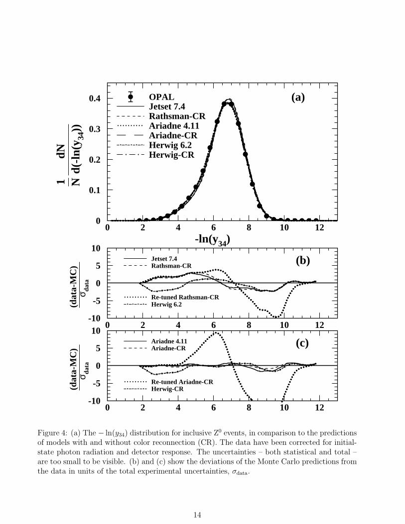
Figure 8: (a) Distribution of ymin in the tagged gluon jets. The distribution includes the effectsof initial-state photon radiation and detector acceptance and resolution. The uncertaintiesare statistical only. The results are shown in comparison to the predictions of QCD MonteCarlo programs which include detector simulation and the same analysis procedures as areapplied to the data. The hatched area shows the quark jet background evaluated using Jetset.(b) Fractional difference between the results of a Monte Carlo program with color reconnectionand the corresponding model without reconnection. To define gluon jets with a rapidity gap,the region ymin≥ 1.4, to the right of the vertical dashed line, is selected.

20

10-3

10-2

10-1

1

0 0.5 1 1.5 2 2.5∆ymax

1 NdN

d(∆y

max

)OPALJetset 7.4Rathsman-CRAriadne 4.11Ariadne-CRHerwig 6.2Herwig-CRQuark jetbackground

(a)

-1

0

1

2

3

4

0 0.5 1 1.5 2 2.5

Selected

∆ymax

δ ∆ym

ax

(Rathsman-CR − Jetset)/Jetset(Ariadne-CR − Ariadne)/Ariadne(Herwig-CR − Herwig)/Herwig

(b)

Figure 9: (a) Distribution of ∆ymax for tagged gluon jets with ymin< 1.4. The distributionincludes the effects of initial-state photon radiation and detector acceptance and resolution. Theuncertainties are statistical only. The results are shown in comparison to the predictions of QCDMonte Carlo programs which include detector simulation and the same analysis procedures asare applied to the data. The hatched area shows the quark jet background evaluated usingJetset. (b) Fractional difference between the results of a Monte Carlo program with colorreconnection and the corresponding model without reconnection. To define gluon jets with arapidity gap, the region ∆ymax ≥ 1.3, to the right of the vertical dashed line, is selected.

21

7.1 Detector level distributions

The charged particle multiplicity distribution of the leading part of the gluon jets, nch.leading,

is shown in Fig. 10a. The results are shown in comparison to the predictions of the Jet-set and Rathsman-CR models. Fig. 10b shows the same data compared to Ariadne andAriadne-CR. The most striking feature of these results is the large excess of entries predicted bythe Ariadne-CR and Rathsman-CR models at nch.

leading =2 and 4 compared to the correspondingmodels without color reconnection. Using Monte Carlo information, we verified these excessesare a consequence of events like Fig. 1b, present in the CR models but not in the models with-out CR. The isolated, electrically neutral gluonic system in the leading part of the gluon jets inthese events decays into an even number of charged particles, yielding the spikes at nch.

leading =2and 4.

The data are generally well described by Jetset (Fig. 10a), except for the bins with nch.leading =

1, 2 and 4 where the data exceed the predictions by more than one standard deviation of thestatistical uncertainties. The description by Ariadne (Fig. 10b) is considerably worse in thatthe data lie well above the Ariadne results for most of the range between nch.

leading =2 and 6.Nonetheless, Jetset and Ariadne provide a much better overall description of the data thanthe corresponding models with reconnection. In particular, there is not a significant “spikingeffect” in the data at even values of multiplicity as predicted by these two CR models. Weconclude that color reconnection as implemented by the Rathsman-CR and Ariadne-CR modelsis strongly disfavored, at least using their standard parameters given in Sect. 3.

The nch.leading distribution obtained using the ymin selection (see Sect. 6) is presented in Fig. 11.

The data are shown in comparison to the corresponding results of the Herwig and Herwig-CRmodels. We use the ymin selection to test Herwig-CR, and not the standard selection defined bythe combined ymin and ∆ymax samples, because the latter is not sensitive to differences betweenthe Herwig and Herwig-CR models as discussed in Sect. 6. For purposes of comparison, theprediction of Herwig using the standard selection is shown in Fig. 10a, however.

From Fig. 11, the Herwig-CR model is seen to predict a systematic excess of entries relativeto the corresponding model without CR for multiplicities between about 2 and 5. The overalldescription of the nch.

leading distribution by the Herwig-CR model is nonetheless reasonable, atleast in comparison to the predictions of Jetset and Ariadne in Fig. 10. The best overalldescription of the nch.

leading distribution is provided by Herwig.

We next sum the charges of the particles in the leading part of the gluon jets to find the totalleading electric charge, Qleading. This type of distribution was suggested in [9]. The distributionof Qleading is shown in Fig. 12a. The Rathsman-CR and Ariadne-CR models are seen to predicta large excess of events with Qleading =0 compared to the data or models without reconnection,due to the presence of electrically neutral isolated gluonic systems at large rapidities as discussedabove. The Jetset and Ariadne predictions for the rate of gluon jets with Qleading =0 are about20% too low. For purposes of comparison, the prediction of Herwig is shown in Fig. 12a. Herwigis seen to describe the data well.

Our measurement of the rate of gluon jets with Qleading =0 therefore lies between the predic-tions of the Jetset and Rathsman-CR models, and similarly between the predictions of Ariadneand Ariadne-CR. In this respect, the data appear to be consistent with the presence of a fi-

22

0

0.005

0.01

0.015

0 2 4 6 8 10 12nleading

ch

1 NdN dn

lead

ing

gap

chOPALJetset 7.4Rathsman-CRHerwig 6.2Quark jetbackground

(a)

0

0.005

0.01

0.015

0 2 4 6 8 10 12nleading

ch

1 NdN dn

lead

ing

gap

ch

OPALAriadne 4.11Ariadne-CRQuark jetbackground

(b)

Figure 10: Distribution of nch.leading in the leading part of gluon jets, based on our standard

selection. “N” represents the total number of selected gluon jets and “Ngap” the number ofgluon jets with a rapidity gap. The distribution includes the effects of initial-state photonradiation and detector acceptance and resolution. The uncertainties are statistical only. Theresults are shown in comparison to the predictions of QCD Monte Carlo programs which includedetector simulation and the same analysis procedures as are applied to the data: (a) the Jetset,Rathsman-CR and Herwig models, and (b) the Ariadne and Ariadne-CR models. The hatchedarea shows the quark jet background evaluated using Jetset in part (a) and Ariadne in part (b).

23

0

0.005

0.01

0.015

0 2 4 6 8 10 12nleading

ch

1 NdN dn

lead

ing

gap

chOPALHerwig 6.2Herwig-CRQuark jetbackground

Figure 11: Distribution of nch.leading in the leading part of gluon jets, based on the ymin selection

(see Sect. 6). “N” represents the total number of selected gluon jets and “Ngap” the numberof gluon jets with a rapidity gap. The distributions include the effects of initial-state photonradiation and detector acceptance and resolution. The results are shown in comparison to thepredictions of the Herwig and Herwig-CR models. The uncertainties are statistical only. Thehatched area shows the quark jet background evaluated using Herwig.

nite amount of color reconnection, at least as predicted by these two CR models, albeit at asignificantly smaller level than predicted by the default CR settings of the models. The mostunambiguous signal for color reconnection in our study is the spiking effect at even valuesof nch.

leading seen in Fig. 10, however. The data do not provide clear evidence for these spikes.Furthermore, the Herwig model without CR describes the Qleading distribution well, as seenfrom Fig. 12a. Therefore, the discrepancies of Jetset and Ariadne with the data in Fig. 12ado not provide unambiguous evidence for reconnection effects, but instead are consistent withother inadequacies in the simulations, not related to CR. The same statement holds for thediscrepancies of Jetset and Ariadne with the data in Fig. 10.

The distribution of Qleading obtained using the ymin selection is presented in Fig. 12b. Thedata are shown in comparison to the corresponding results from Herwig and Herwig-CR. Herwigdescribes the data well, similar to Fig. 12a. The predictions of the Herwig-CR model are seento lie somewhat above the data, especially for Qleading =0 and 1.

As a systematic check, we repeated the analysis presented above using different choices forthe scale of gluon jets, κjet, see eq. (1). Specifically we examined the results for 4<κjet< 7 GeVand κjet< 4 GeV, rather than κjet> 7 GeV as in our standard analysis. Note the definition ofa gluon jet becomes ambiguous for small κjet values. We find that the spikes at even values ofnch.leading predicted by the Rathsman-CR and Ariadne-CR models become much less prominent

24

0

0.01

0.02

0.03

0.04

-4 -3 -2 -1 0 1 2 3 4 5Qleading

1 NdN dQ

lead

ing

gap

OPALJetset 7.4Rathsman-CRAriadne 4.11Ariadne-CRHerwig 6.2Quark jetbackground

(a)

0

0.005

0.01

0.015

0.02

0.025

-4 -3 -2 -1 0 1 2 3 4 5Qleading

1 NdN dQ

lead

ing

gap

OPALHerwig 6.2Herwig-CRQuark jetbackground

(b)

Figure 12: Distribution of Qleading in the leading part of gluon jets in comparison to the pre-dictions of QCD Model Carlo programs: (a) using the standard selection; (b) using the ymin

selection. “N” represents the total number of selected gluon jets and “Ngap” the number ofgluon jets with a rapidity gap. For both parts (a) and (b), the distributions include the effectsof initial-state photon radiation and detector acceptance and resolution. The uncertainties arestatistical only. The hatched area shows the quark jet background evaluated using Herwig.

25

for the smaller κjet scales, especially the spike at nch.leading =4, i.e. the selections with softer

or more collinear gluon jets are less sensitive to color reconnection. This justifies the choiceκjet > 7 GeV for our standard analysis. To the extent that a CR signal is still visible using thesmaller κjet ranges, we find that the values of ymin and ∆ymax above which the predictions of theCR models exhibit deviations from the non-CR models are similar to those shown in Figs. 8band 9b.

As an additional check, we repeated the analysis described in Sects. 5 and 6 except usingenergy ordering to identify gluon jets rather than secondary vertex reconstruction. In theenergy ordering method, the jet with the smallest calculated energy in three-jet qqg events isassumed to be the gluon jet. The purity of gluon jets identified using this technique is muchlower than found using secondary vertices, especially for the high energy jets most sensitive tocolor reconnection. The gluon jet purity found using energy ordering is 64%, compared to 95%for our standard analysis. To increase the purity, we therefore required Ejet< 15 GeV, ratherthan Ejet< 35 GeV as in the standard analysis. This method yields about 94 000 tagged gluonjets. The mean gluon jet energy is 12.9 GeV and the estimated purity 81%. After imposing therapidity gap requirements of Sect. 6, we obtain 6604 gluon jets with an estimated purity of 56%.The results we obtain from this check are consistent with our observations presented above.In particular, the results for the Qleading distribution are qualitatively similar to those shownin Fig. 12. We note, however, that the spike at nch.

leading =4 predicted by the Rathsman-CRand Ariadne-CR models in Fig. 10 is not visible in the corresponding Monte Carlo predictionsbased on energy ordering, because of their softer energy scales (i.e. this is similar to the checkemploying smaller κjet values, mentioned above). Therefore the selection using energy orderingis not as sensitive to color reconnection as our standard selection.

The results of Figs. 10–12 demonstrate the sensitivity of our study to processes with colorreconnection. We discuss the effect of parameter variation on the predictions of the Rathsman-CR and Ariadne-CR models in Sect. 7.4.

7.2 Correction procedure

As the next step in our study, we correct the data in Figs. 10–12 to the hadron level. Thecorrection procedure employs an unfolding matrix. The matrix is constructed using detectorlevel Monte Carlo events. The events are subjected to the detector level requirements of Sects. 2and 5. In addition, the events are required to exhibit a rapidity gap, defined by the conditionsof Sect. 6, at both the detector and hadron levels. The matrices relate the values of nch.

leading

and Qleading at the detector level to the corresponding values before the same event is processedby the detector simulation. Thus the matrices correct the data to the hadron level with theexception that initial-state radiation and the experimental event acceptance are included. Ina second step, the data are corrected for event acceptance, initial-state radiation, and gluonjet impurity using bin-by-bin factors. The matrices and bin-by-bin factors are determinedusing Herwig because the data in Figs. 10–12 are best described by that model. Statisticaluncertainties are evaluated for the corrected data using propagation of errors, including thestatistical uncertainties of the correction factors.

Because of finite acceptance, especially for soft particles, significantly more events satisfy therapidity gap requirements at the detector level than at the hadron level. As a consequence, the

26

overall corrections are fairly large, of the order of 40%. To verify the reliability of the correctionprocedure, we therefore performed the following test. We treated our sample of Jetset eventsat the detector level as “data,” using the Herwig derived corrections to unfold them. Thecorrected Jetset distributions were found to agree with the corresponding Jetset distributionsgenerated at the hadron level to within the statistical uncertainties. This demonstrates thatour correction procedure does not introduce a significant bias.

To evaluate systematic uncertainties for the corrected data, we repeated the analysis usingthe three systematic variations listed in Sect. 4, with one exception: to determine the systematicuncertainty related to the model dependence of the correction factors, we repeated the analysisusing the Jetset, Ariadne and Herwig-CR models only. We did not include the Rathsman-CRor Ariadne-CR model because of their poor description of the data, see Figs. 10 and 12a. Inaddition, we made the following change to the standard analysis to assess the effect of alteringthe criteria used to identify gluon jets.

• To identify the lower energy quark jets, we required the decay length to satisfy L/σL > 3rather than L/σL > 5; this resulted in 1002 tagged gluon jets which satisfied the rapiditygap requirements, with an estimated purity of 76%.

The systematic uncertainties were treated as described in Sect. 4, i.e. the full differences of theresults of the systematic checks with respect to the standard analysis defined the systematicuncertainty for each term, and the individual terms were added in quadrature to define thetotal systematic uncertainties.

The largest contributions to the total systematic uncertainties arose from using Ariadne todetermine the correction factors, followed by the requirement L/σL > 3 to identify the lowerenergy quark jets.

7.3 Hadron level distributions

The corrected distributions of nch.leading and Qleading are presented in Fig. 13. These results are

based on our standard selection, i.e. the ymin and ∆ymax samples added together. The dataare shown in comparison to the hadron level predictions of the Jetset, Rathsman-CR, Ariadneand Ariadne-CR models. For purposes of comparison, the predictions of Herwig are shownas well. The qualitative features of the predictions are seen to be similar to those of thecorresponding detector level distributions in Figs. 10 and 12a. In particular, the Ariadne-CRand Rathsman-CR models exhibit a large excess of entries at nch.

leading =2 and 4 in Fig. 13a,corresponding to the Qleading =0 bin in Fig. 13b, analogous to the results of Sect. 7.1. FromFig. 13a it is also seen that the Rathsman-CR model predicts a spike at nch.

leading =6. This latterfeature was not apparent in the detector level distribution of Fig. 10a because of finite detectorresolution.

The corresponding results based on the ymin sample are presented in Fig. 14. The data areshown in comparison to the predictions of the Herwig and Herwig-CR models. From Fig. 14ait is seen that the Herwig-CR model predicts a significant excess of events relative to Herwigfor nch.

leading =2, 4 and 6, analogous to the results of the Rathsman-CR and Ariadne-CR models

27

in Fig. 13a. This suggests that the production of events like Fig. 1b is a general feature of colorreconnection. The spike in the prediction of the Herwig-CR model at nch.

leading=4 in Fig. 14aprobably explains the general excess of the Herwig-CR results above Herwig for multiplicitiesbetween nch.

leading=3 and 5 in Fig. 11.

7.4 Effect of parameter variation on the model predictions

We next study the effect of parameter variation on the predictions of the Rathsman-CR andAriadne-CR models, to determine if they can be tuned to describe the gluon jet data of Fig. 13without adversely affecting their descriptions of the inclusive Z0 decay measurements presentedin Sect. 4.

To begin, we define ∆QMC−dataleading to be the difference between the Monte Carlo prediction and

experimental result for the Qleading =0 bin in Fig. 13b. We then vary the principal parametersof the models one at a time, with the other parameters at their standard values, to see if itis possible to reduce ∆QMC−data

leading to zero or near-zero, i.e. to obtain agreement of the model’s

prediction with this measurement. We note that if ∆QMC−dataleading is near-zero, the predictions of

the model for the nch.leading distribution in Fig. 13a will also be in general agreement with the

data since the events which yield the excess of entries in Fig. 13b are the same as those whichyield the excess in Fig. 13a.

The Rathsman-CR model: For the Rathsman-CR model, the following parameters werevaried:

• ΛQCD, the QCD scale parameter, given by PARJ(81);

• Q0, the minimum mass value to which partons evolve, given by PARJ(82);

• a and b, which control the longitudinal momentum spectrum of hadrons relative to thestring direction in the Lund model of hadronization, given by PARJ(41) and PARJ(42);

• σq, which controls the transverse momentum spectrum of hadrons, given by PARJ(21).

The PARJ references are the names of the parameters in the Pythia Monte Carlo. These fiveparameters are the most important ones controlling the multiplicity and momentum distribu-tions of hadrons in the model. Note we do not include the color reconnection suppression factorR0 mentioned in Sect. 3 in the above list. It is a trivial result that the Rathsman-CR modelwill describe the data as well as Jetset for R0 → 0 since the two models are identical in thislimit. Varying R0 to reproduce the experimental result and corresponding uncertainty for theQleading =0 bin in Fig. 13b yields R0 =0.0085± 0.0075 (stat.)± 0.0087 (syst.), consistent withR0 =0.

The results for ∆QMC−dataleading are shown in Fig. 15. The standard values of the parameters

are indicated by solid dots. The uncertainties attributed to the parameter values in [23],beyond which the description of inclusive Z0 measurements is significantly degraded if the

28

0

0.005

0.01

0.015

0 2 4 6 8 10 12nleading

ch

1 NdN dn

lead

ing

gap

ch

OPALJetset 7.4Rathsman-CRHerwig 6.2Ariadne 4.11Ariadne-CR

(a)

0

0.01

0.02

0.03

-4 -3 -2 -1 0 1 2 3 4 5Qleading

1 NdN dQ

lead

ing

gap

OPALJetset 7.4Rathsman-CRHerwig 6.2Ariadne 4.11Ariadne-CR

(b)

Figure 13: Distributions of (a) nch.leading and (b) Qleading in the leading part of gluon jets, based

on our standard selection. “N” represents the total number of selected gluon jets and “Ngap”the number of gluon jets with a rapidity gap. The data have been corrected for initial-statephoton radiation, gluon jet impurity, and detector response. The horizontal bars indicate thestatistical uncertainties. The vertical lines show the total uncertainties, with statistical andsystematic terms added in quadrature. The results are shown in comparison to the predictionsof QCD Monte Carlo models.

29

0

0.002

0.004

0 2 4 6 8 10 12

(a)

nleadingch

1 NdN dn

lead

ing

gap

ch

OPAL

Herwig 6.2

Herwig-CR

0

0.002

0.004

0.006

0.008

0.01

-4 -3 -2 -1 0 1 2 3 4 5

(b)

Qleading

1 NdN dQ

lead

ing

gap

OPAL

Herwig 6.2

Herwig-CR

Figure 14: Distributions of (a) nch.leading and (b) Qleading in the leading part of gluon jets, based

on the ymin selection. “N” represents the total number of selected gluon jets and “Ngap” thenumber of gluon jets with a rapidity gap. The data have been corrected for initial-state photonradiation, gluon jet impurity, and detector response. The horizontal bars indicate the statisticaluncertainties. The vertical lines show the total uncertainties, with statistical and systematicterms added in quadrature. The results are shown in comparison to the predictions of theHerwig and Herwig-CR Monte Carlo models.

30

other parameters remain at their standard values, are indicated by the horizontal error ranges.Note that an uncertainty is not evaluated for the a parameter in [23] and that the uncertaintiesattributed to ΛQCD and b are too small to be visible. The width of the shaded bands in Fig. 15indicates twice the total experimental uncertainty of ∆QMC−data

leading , corresponding to plus andminus one standard deviation.

It is seen that ∆QMC−dataleading can be reduced to zero for ΛQCD≈ 1.3 GeV. As ΛQCD is increased,

more soft gluons are produced, increasing the probability for multiple color reconnections in anevent. In events with multiple reconnections, color strings can reconnect the isolated gluonicstring segment illustrated in Fig. 1b back with the rest of the event, spoiling the rapidity gap.From Fig. 15 it is also seen that ∆QMC−data

leading can be reduced to near-zero for large values of Q0,e.g. Q0 ∼

> 4 GeV/c2. As Q0 is increased, fewer soft gluons are available, effectively decreasingthe reconnection probability. In this sense, an increase in the value of Q0 is analogous to areduction in the value of the parameter R0 discussed above. We note that the values of ΛQCD

and Q0 required to reduce ∆QMC−dataleading to zero or near-zero represent large excursions from their

standard values. Fig. 15 suggests it is unlikely that ∆QMC−dataleading can be reduced to zero or

near-zero through variation of a or σq.

Setting Q0 to 3.5 GeV/c2 with the other parameters at their standard values, the Rathsman-CR model predicts a mean charged multiplicity in inclusive Z0 events of 〈nch.〉=20.2, smallerthan the experimental result of 21.15 ± 0.29 mentioned in Sect. 4. Mean multiplicity in theLund hadronization model is primarily controlled by the parameters a and b. Therefore, havingset Q0 =3.5 GeV/c2, we varied the b parameter7 to reproduce the measured result for 〈nch.〉.To increase the prediction for 〈nch.〉, b needs to be decreased. As b decreases, ∆QMC−data

leading alsotends to become smaller (see Fig. 15d). By iterating the adjustment of Q0 and b, it thereforeproved possible to simultaneously obtain ∆QMC−data

leading ≈ 0 and 〈nch.〉≈ 21.15. The result we find

for the two parameters is Q0 =5.5 GeV/c2 and b=0.27 GeV−2, corresponding to ∆QMC−dataleading =

6.7 × 10−7. We refer to the Rathsman-CR model with these adjusted parameters as the “re-tuned” Rathsman-CR model.

A one standard deviation limit was evaluated for the re-tuned parameters by adjusting Q0

and b so they yielded the correct result for 〈nch.〉 and agreement with the one standard deviationupper limit for ∆QMC−data

leading shown in Fig. 15: the result is Q0=3.7 GeV/c2 and b=0.35 GeV−2.A two standard deviation limit was evaluated in an analogous manner, based on twice the totaluncertainty of ∆QMC−data

leading : the result is Q0 =3.2 GeV/c2 and b=0.38 GeV−2. Finally, Q0 and

b were adjusted to yield ∆QMC−dataleading ≈ 0 and a value for 〈nch.〉 equal to the LEP-averaged result

plus its one standard deviation uncertainty, specifically 〈nch.〉=21.44, see above and Sect. 4.The result is Q0=5.2 GeV/c2 and b=0.25 GeV−2.

We examined the description of the re-tuned Rathsman-CR model for the inclusive Z0

measurements in Figs. 2–5. The total χ2 for the 81 bins of data was found to be 1117.7,much larger than the result χ2=243.5 presented in Sect. 4 for the standard version of theRathsman-CR model (see Table 3). Using the one and two standard deviation limits for there-tuned parameters, given above, the corresponding χ2 are 435.1 and 327.2 respectively, stillsignificantly larger than the χ2 of the standard version. The χ2 result for the parameters tunedto yield 〈nch.〉=21.44 is 785.2.

7The a and b parameters are highly correlated with respect to the model predictions for 〈nch.〉; therefore weconsider variation of the b parameter alone, not both a and b.

31

-0.02

0

0.02

0.04

0 1 2 3

∆QM

C-d

ata

lead

ing

ΛQCD (GeV)

(a)

-0.02

0

0.02

0.04

0 2 4 6Q0 (GeV/c2)

(b)

-0.02

0

0.02

0.04

0 1 2 3

∆QM

C-d

ata

lead

ing

a

(c)

-0.02

0

0.02

0.04

0.06

0 1 2 3 4 5b (GeV-2)

(d)

-0.02

0

0.02

0.04

0 0.2 0.4 0.6 0.8 1

∆QM

C-d

ata

lead

ing

σq (GeV/c)

(e)Rathsman-CR

versus data

Figure 15: Results for the difference between the Rathsman-CR Monte Carlo prediction andthe experimental result for the Qleading =0 bin in Fig. 13b, ∆QMC−data

leading , as the principal pa-rameters of the model are changed with the other parameters at their default settings. Thesolid dots indicate the standard values of the parameters. The horizontal error ranges showthe uncertainties attributed to the parameter values in [23]. For the parameters ΛQCD and b,these uncertainties are too small to be visible. Note an uncertainty is not evaluated for the aparameter. The width of the shaded band centered on ∆QMC−data

leading =0 equals twice the total

experimental uncertainty of ∆QMC−dataleading .

32

The χ2 results for the re-tuned Rathsman-CR model are listed in the bottom portion ofTable 3. The deviations of the re-tuned model from the measured distributions are shown bythe dotted curves in part (b) of Figs. 2–5.

We attempted to follow an analogous procedure to that described above for Q0 to ad-just ΛQCD. With ΛQCD set to 1.3 GeV and the other parameters at their standard values, themean charged multiplicity of inclusive Z0 events is 26.4. To reduce this to 21.15, we increasedthe value of b. As b increases, ∆QMC−data

leading becomes larger, however (Fig. 15d), and we could

not find a solution which yielded both ∆QMC−dataleading ≈ 0 and 〈nch.〉≈ 21.15. The closest solution

we found, defined by the set of parameters which provided the correct inclusive multiplicityand a minimal result for ∆QMC−data

leading , was ΛQCD=1.3 GeV and b=4.9 GeV−2, which yielded

∆QMC−dataleading =0.012, with χ2=2.1× 104 for the data of Figs. 2–5.

Last, motivated by the observation that larger values of ΛQCD andQ0 both reduce ∆QMC−dataleading

while having opposite effects on 〈nch.〉, we increased both ΛQCD and Q0, with the other param-eters at their standard values, to search for a solution with ∆QMC−data

leading ≈ 0 and 〈nch.〉≈ 21.15.Specifically, we systematically increased the value of ΛQCD and then performed a scan to de-termine the value of Q0 which yielded the correct result for 〈nch.〉. The parameter set withthe minimal result for ∆QMC−data

leading was ΛQCD=0.6 GeV and Q0 =4.9 GeV/c2, which yielded

∆QMC−dataleading =0.004, with χ2=1606 for the data of Figs. 2–5.

We conclude it is unlikely that the gluon jet results of Sect. 7.3 can be reproduced by theRathsman-CR model through variation of ΛQCD, similar to our observation above for a and σq.

Thus, the only mechanism we found to adjust the parameters of the Rathsman-CR modelto simultaneously describe our data on rapidity gaps in gluon jets and 〈nch.〉 in inclusive Z0

decays was to increase Q0 to values in the range from about 3.3 to 5.5 GeV/c2, much largerthan the values of 1–2 GeV/c2 normally attributed to this parameter. These large values of Q0

resulted in a significant degradation of the model’s description of inclusive Z0 events, however,as discussed above. We conclude it is unlikely that this model can simultaneously provide asatisfactory description of the data in Sects. 4 and 7.3 using its standard value for the strengthof color reconnection, R0=0.1. Thus, our results provide compelling evidence to disfavor colorreconnection as it is currently implemented by this model.

The Ariadne-CR model: The following parameters of the Ariadne-CR model were variedto determine their influence on ∆QMC−data

leading :

• ΛQCD, given by PARA(1);

• pT,min., the minimum transverse momentum of a gluon with respect to the dipole whichemits it, given by PARA(3);

• a, b and σq, given by PARJ(41), PARJ(42) and PARJ(21) as for the Rathsman-CR model.

The PARA references are the names of the parameters in Ariadne, see Table 2. Analogous to ourtreatment of the Rathsman-CR model, we do not include the color suppression factor PARA(26)

33

(see Sect. 3) in this list. Varying PARA(26) to reproduce the result for the Qleading =0 bin inFig. 13b, as well as the result for the Qleading =0 bin plus its one standard deviation totaluncertainty, yields PARA(26)= 96 and 41, respectively, much larger than the standard valuePARA(26)= 9. Note that large values of PARA(26) correspond to the limit of large NC inwhich the probability for color reconnection becomes negligible.

The results are shown in Fig. 16. The standard parameter values are indicated by soliddots. Their uncertainties as given in Table 2 are too small to be visible in the figure. Notean uncertainty was not evaluated for the a or σq parameters. Also note the Ariadne computerprogram requires ΛQCD<pT,min.. For this reason, the results for ΛQCD are shown up to 0.70 GeVonly, which is the standard value of pT,min..

The results of Fig. 16 are similar to those of Fig. 15, i.e. ∆QMC−dataleading approaches zero as

the parton shower cutoff pT,min. is increased from its standard value, while it exhibits the samebehavior shown in Fig. 15 as a, b and σq are varied.

Setting pT,min.=2 GeV/c so that ∆QMC−dataleading ≈ 0 (see Fig. 16b), with the other parameters

at their standard values, 〈nch.〉 in inclusive Z0 decays is predicted to be 20.0. Through iterativeadjustment of pT,min. and b, we found ∆QMC−data

leading ≈ 0 (specifically, ∆QMC−dataleading =−4.1 × 10−5)

and 〈nch.〉≈ 21.15 for pT,min.=4.7 GeV/c and b=0.17 GeV−2. We refer to the Ariadne-CRmodel with these adjusted parameters as the “re-tuned” Ariadne-CR model. One and twostandard deviation limits were evaluated for the re-tuned parameters in the same manner asdescribed above for the re-tuned Rathsman-CR model; the results are pT,min.=2.0 GeV/c andb=0.35 GeV−2, and pT,min.=1.5 GeV/c and b=0.42 GeV−2, respectively. Similarly, we tunedpT,min. and b to yield ∆QMC−data

leading ≈ 0 and 〈nch.〉=21.44, analogous to the procedure in Sect. 7.4:this yielded pT,min.=3.5 GeV/c and b=0.20 GeV−2.

Using the re-tuned parameters to determine the predictions of the model for the data inFigs. 2–5 resulted in a total χ2 of 3019.3 for those distributions, compared to the result χ2=32.4presented in Sect. 4 for the standard version of Ariadne-CR (Table 3). For the one and twostandard deviation re-tuned parameters, the corresponding results are χ2=333.1 and 132.6,respectively. Thus the description provided by the re-tuned model is much worse than thatprovided by the standard version, even considering the uncertainties of the re-tuned parameterset. For the parameters tuned to yield 〈nch.〉=21.44, the corresponding χ2 is 1254.6.

The χ2 results for the re-tuned Ariadne-CR model are listed in the bottom portion ofTable 3. The deviations of the re-tuned model from the measured distributions are shown bythe dotted curves in part (c) of Figs. 2-5.

Analogous to the procedure we followed for the Rathsman-CR model, we also attemptedto simultaneously describe our gluon jet data and 〈nch.〉 in inclusive Z0 decays by varyingboth ΛQCD and pT,min. with the other parameters at their standard values. The solution whichyielded the minimal result for ∆QMC−data

leading while correctly describing 〈nch.〉 was ΛQCD=0.5 GeV

and pT,min.=2.4 GeV/c, which yielded ∆QMC−dataleading =0.0041, with χ2=2095 for the data of

Figs. 2–5. We did not attempt an adjustment of the two parameters ΛQCD and b as we did forthe Rathsman-CR model since the value of ΛQCD is constrained by pT,min. as explained above.

Thus the only manner we found to adjust the parameters of the Ariadne-CR model todescribe our data on gluon jets with a rapidity gap and at the same time yield 〈nch.〉≈ 21.15

34

-0.02

0

0.02

0.04

0 1 2 3

∆QM

C-d

ata

lead

ing

ΛQCD (GeV)

(a)limit from

pT,min

-0.02

0

0.02

0.04

0 2 4 6pT,min (GeV/c)

(b)

-0.02

0

0.02

0.04

0 1 2 3

∆QM

C-d

ata

lead

ing

a

(c)

-0.02

0

0.02

0.04

0 1 2 3 4 5b (GeV-2)

(d)

-0.02

0

0.02

0.04

0 0.2 0.4 0.6 0.8 1

∆QM

C-d

ata

lead

ing

σq (GeV/c)

(e)Ariadne-CRversus data

Figure 16: Results for the difference between the Ariadne-CR Monte Carlo prediction and theexperimental result for the Qleading =0 bin in Fig. 13b, ∆QMC−data

leading , as the principal parametersof the model are changed with the other parameters at their default settings. The solid dotsindicate the standard values of the parameters. The uncertainties attributed to the parametervalues in Table 2 are too small to be visible. Note an uncertainty is not evaluated for the aor σq parameters. The width of the shaded band centered on ∆QMC−data

leading =0 equals twice the

total experimental uncertainty of ∆QMC−dataleading .

35

was to increase the parton shower cutoff parameter pT,min. to values in the range from about 1.6to 4.7 GeV/c, significantly larger than the range of 0.6–0.7 GeV/c normally attributed to thisparameter. This resulted in a significant degradation of the model’s description of the globalproperties of inclusive Z0 events as described above. Analogous to the Rathsman-CR model,we conclude it is unlikely that the Ariadne-CR model can simultaneously provide a satisfactorydescription of the data in both Sects. 4 and 7.3 using its standard value for the strength ofcolor reconnection, and that our results provide compelling evidence to disfavor this model.

8 Search for glueball-like resonances

Besides providing a sensitive means to test models of color reconnection, gluon jets with arapidity gap present an environment which may favor the production of glueballs, as discussedin [9]. If a hard, acollinear gluon in a e+e− three-jet qqg event propagates a significant distancewithout radiating, a rapidity gap can form between the gluon jet and the rest of the event.This could enhance the probability for a color octet field to be created between the gluon andresidual qq system, see Fig. 17a. This octet field is analogous to the field which is expected toconnect two separating gluons produced in a color singlet state. This is in contrast to e.g. theLund hadronization model, in which only color triplet fields are present, see Fig. 17b. Coloroctet fields provide a natural environment in which to create glueballs [40], through gg pairproduction from the vacuum, see Fig. 17c.

QCD lattice calculations and other sources (see [41] and references therein) suggest that themass of the lightest glueball state should lie in the general range from about 1 to 2 GeV/c2.One of the main candidates for the lightest glueball is the f0(1500) [42], with a resonance widthof 0.11 GeV/c2. The principal charged particle decay modes of the f0(1500) are π+π− andπ+π−π+π−.

Following the suggestions in [9], we therefore examine invariant mass spectra in the leadingpart of our selected gluon jets. Since we are searching for anomalous resonant structure, thedata are compared to the predictions of the models without color reconnection, i.e. Jetset,Ariadne and Herwig. These models do not contain glueballs. The distributions are examinedat the detector level only and are normalized to the number of entries in the distributions.The bin widths are adjusted to reflect the mass resolution of the detector, estimated from thesimulations.

We begin by examining the total invariant mass of the leading part of the gluon jets, Mleading.These masses are determined using both charged and neutral particles. Charged particles areassumed to be pions and neutral particles photons, as stated in Sect. 2. Since glueballs areelectrically neutral, we select gluon jets with Qleading =0, see Fig. 12a. Of the sample of 655events discussed in Sect. 6, this yields 250 gluon jets. The Mleading distribution of these jets ispresented in Fig. 18a. The data are shown in comparison to the corresponding results of Jetset,Ariadne and Herwig. The models are seen to describe the data reasonably well. There is ageneral excess of the data above the Monte Carlo predictions for three bins in the mass rangefrom 1.0 to 2.5 GeV/c2. The total χ2 values with respect to the data for these three bins are11.5 for Jetset, 7.3 for Herwig and 6.0 for Ariadne. Since this excess is only about two standard

36

−

q

q

g

(a) (b)

q−

q

g

−q

q

g g g

glueball

{

(c)

Figure 17: (a) Schematic illustration of a three-jet qqg event with a color octet field stretchedbetween the gluon g and residual quark-antiquark qq system. The double line with hatching,attached to the gluon, represents the octet field. The single lines connecting the octet field tothe quark and antiquark represent color triplet fields. (b) Illustration of a qqg event in whichcolor triplet fields connect the gluon directly with the quark and antiquark. (c) The octet fieldcan be neutralized by the production of virtual gg color singlets from the vacuum, leading tothe formation of glueballs.

deviations of the statistical uncertainties above the predictions of Herwig and Ariadne8, it isnot possible to obtain a definite conclusion concerning this discrepancy.

Motivated by the charged particle decay modes of the f0(1500), mentioned above, we alsoexamine the distributions of invariant mass of two oppositely charged particles in the leadingpart of the gluon jets, M+−

leading, and the corresponding distribution of four charged particleswith total electric charge zero, M+−+−

leading . The simulations predict that about 75% of the chargedparticles in the leading part of the selected gluon jets are pions. The distributions of M+−

leading

and M+−+−leading are presented in Figs. 18b and c. Since in this case the glueball candidate does

not necessarily comprise the entire leading part of the gluon jet, there is no reason to constrainQleading to be zero. Therefore, the M+−

leading and M+−+−leading distributions are based on the entire

sample of 655 gluon jets with a rapidity gap, not just the jets with Qleading =0. Again, thesimulations are seen to describe the data reasonably well. The most significant excess of dataabove the Monte Carlo predictions occurs in the tail of the M+−+−

leading distribution, at massvalues between 2.5 and 3.0 GeV/c2. This excess is about two standard deviations of thestatistical uncertainties above the predictions of Ariadne and somewhat larger for the othermodels. Therefore, we do not observe clear evidence for anomalous resonant structure. Notethe spike in the Herwig prediction for M+−

leading ≈ 0.77 GeV/c2 in Fig. 18b is due to the ρ mesonresonance which is too narrow in Herwig. Jetset exhibits a similar effect but at a less significant

8The Monte Carlo results are based on about twice as many events as the experimental distributions, seeSects. 2 and 3.

37

0

0.2

0.4

0 1 2 3 4 5 6 7 8Mleading (GeV/c2)

1 NdN dM

lead

ing OPAL

Jetset 7.4Ariadne 4.11Herwig 6.2Quark jetbackground

(a)

0

2

0.2 0.4 0.6 0.8 1 1.2 1.4 1.6 1.8M

leading

+- (GeV/c2)

1 NdN dM

lead

ing

+-

OPALJetset 7.4Ariadne 4.11Herwig 6.2Quark jetbackground

(b)

0

1

0.5 1 1.5 2 2.5 3 3.5 4M

leading

+-+- (GeV/c2)

1 NdN dM

lead

ing

+-+-

OPALJetset 7.4Ariadne 4.11Herwig 6.2Quark jetbackground

(c)

Figure 18: Distribution of jet invariant mass based on charged and neutral particles in theleading part of gluon jets. The distribution includes the effects of initial-state photon radiationand detector acceptance and resolution. The uncertainties are statistical only. The results areshown in comparison to the predictions of QCD Monte Carlo programs which include detectorsimulation and the same analysis procedures as are applied to the data. The hatched areashows the quark jet background evaluated using Herwig.

38

level.

To better isolate a signal from a scalar particle such as the f0(1500), we also examinedthe cos θ∗ distribution of charged particle pairs in the leading part of the gluon jets, definedas follows. A “parent” momentum is defined by summing the momenta of two oppositelycharged particles. θ∗ is the angle between the either of the two “decay” particles and theparent momentum, in the rest frame of the parent. The distribution of cos θ∗ should be flatfor a scalar particle but not necessarily for the combinatoric background. The measured cos θ∗

distribution was found to be well described by the Monte Carlo simulations. Therefore, we donot obtain any evidence for the anomalous production of scalar particles.

9 Summary and conclusion

A sample of 12 611 gluon jets with a mean energy of 22 GeV and estimated purity of 95% isidentified in e+e− hadronic Z0 decay events using b quark jet tagging. The data were collectedwith the OPAL detector at LEP. A subsample of about 5% of these jets is selected whichexhibit a rapidity gap, i.e. an absence of charged and neutral particles over a significant rangeof rapidity as illustrated in Fig. 7. After imposing the rapidity gap requirement, the estimatedpurity of the gluon jets is 86%.

We examine the predictions of three models of color reconnection (CR): the Lonnbladmodel [25] (see also [28]) implemented in the Ariadne Monte Carlo, the Rathsman model [27]implemented in the Pythia Monte Carlo, and the color reconnection model in the Herwig MonteCarlo [18]. We refer to these as the Ariadne-CR, Rathsman-CR, and Herwig-CR models, re-spectively. Specifically, we examine the predictions of these models for the distributions ofcharged particle multiplicity and total electric charge in the leading part of the gluon jets,defined by charged and neutral particles beyond the gap.

We find that the Rathsman-CR and Ariadne-CR models predict a large excess of gluon jetswith a rapidity gap, for which the leading part of the jets is electrically neutral, compared tothe corresponding models without color reconnection. In particular, these two models predictlarge spikes in the charged particle multiplicity distribution at even values of multiplicity.Thus our analysis is very sensitive to CR effects. We adjust the principal parameters of thetwo models to determine if they can be tuned to simultaneously provide a good descriptionof our gluon jet measurements and the global properties of inclusive events in hadronic Z0

decays. We find we can obtain a satisfactory description of the gluon jet data and the meancharged particle multiplicity 〈nch.〉 in inclusive Z0 events only for very large values of the partonshower cutoff parameters, Q0≈ 3.2–5.5 GeV/c2 for the Rathsman-CR model or pT,min.≈ 1.5–4.7 GeV/c for the Ariadne-CR model, and that the overall description of global distributionsin inclusive Z0 events is then severely degraded. We conclude that it seems unlikely that eitherof these two models can be tuned to provide a satisfactory description of both our gluon jetdata and the global properties of Z0 events, using their standard values for the strength ofcolor reconnection. We therefore conclude that color reconnection as currently implemented inthese models is disfavored. Our conclusion for the Ariadne-CR model is consistent with ourprevious results [11]. Here, we present an even more sensitive study of color reconnection andsystematically examine the effects of parameter variation on the model’s predictions.

39

The Herwig-CR model also predicts a significant excess of events at even values of chargedparticle multiplicity in the leading part of gluon jets, compared to the corresponding modelwithout color reconnection, cf. Fig. 14a. These excesses are much less prominent than for theRathsman-CR and Ariadne-CR models, however, and are not clearly visible once the effectsof finite detector resolution are incorporated, cf. Fig. 11. Therefore, we are unable to obtaina definite conclusion concerning this model. The data are nonetheless better described by theversion of Herwig without color reconnection.

Our study is also potentially sensitive to the presence of color singlet, electrically neutralobjects such as glueballs, see [9]. We therefore examine the total invariant mass distribution ofthe leading part of gluon jets, using events in which the leading system is electrically neutral.We also examine the invariant mass distributions of two oppositely charged particles, and of fourcharged particles with total electric charge zero, in the leading part of our sample of gluon jets.We do not observe any evidence for anomalous features in the data, including the productionof glueball-like objects.

10 Acknowledgments

We particularly wish to thank the SL Division for the efficient operation of the LEP acceleratorat all energies and for their close cooperation with our experimental group. In addition to thesupport staff at our own institutions we are pleased to acknowledge the

Department of Energy, USA,National Science Foundation, USA,Particle Physics and Astronomy Research Council, UK,Natural Sciences and Engineering Research Council, Canada,Israel Science Foundation, administered by the Israel Academy of Science and Humanities,Benoziyo Center for High Energy Physics,Japanese Ministry of Education, Culture, Sports, Science and Technology (MEXT) and a grantunder the MEXT International Science Research Program,Japanese Society for the Promotion of Science (JSPS),German Israeli Bi-national Science Foundation (GIF),Bundesministerium fur Bildung und Forschung, Germany,National Research Council of Canada,Hungarian Foundation for Scientific Research, OTKA T-038240, and T-042864,The NWO/NATO Fund for Scientific Research, the Netherlands.

40

References

[1] S. Brandt et al., Phys. Lett. 12 (1964) 57;E. Fahri, Phys. Rev. Lett. 39 (1977) 1587.

[2] J.D. Bjorken, Phys. Rev. D47 (1993) 101.

[3] H1 Collab., T. Ahmed et al., Nucl. Phys. B429 (1994) 477;ZEUS Collab., M. Derrick et al., Phys. Lett. B332 (1994) 228;ZEUS Collab., M. Derrick et al., Phys. Lett. B369 (1996) 55.

[4] D0 Collab., S. Abachi et al., Phys. Rev. Lett. 72 (1994) 2332;CDF Collab., F. Abe et al., Phys. Rev. Lett. 74 (1995) 855;D0 Collab., B. Abbott et al., Phys. Lett. B440 (1998) 189;CDF Collab., T. Affolder et al., Phys. Rev. Lett. 85 (2000) 4215.

[5] For a recent review, see A.B. Kaidalov, in M. Shifman and B. Ioffe (eds.), “At the frontier

of particle physics,”, vol. 1, Singapore: World Scientific (2001), p. 603, e-Print Archive:hep-ph/0103011; for a discussion of the pomeron in the context of rapidity gaps, see A.Hebecker, Phys. Rep. 331 (2000) 1.

[6] B. Andersson et al., Phys. Rep. 97 (1983) 31.

[7] G. Gustafson, U. Pettersson and P.M. Zerwas, Phys. Lett. B209 (1988) 90.

[8] OPAL Collab., G. Abbiendi et al., Phys. Lett. B453 (1999) 153;L3 Collab., M. Acciarri et al., Phys. Lett. B454 (1999) 386;ALEPH Collab., B. Barate et al., Eur. Phys. J. C17 (2000) 241;DELPHI Collab., P. Abreu et al., Phys. Lett. B511 (2001) 159.

[9] P. Minkowski and W. Ochs, Phys. Lett. B485 (2000) 139.

[10] SLD Collab., K. Abe et al., Phys. Rev. Lett. 76 (1996) 4886.

[11] OPAL Collab., G. Abbiendi et al., Eur. Phys. J. C11 (1999) 217.

[12] OPAL Collab., K. Ahmet et al., Nucl. Instr. and Meth. A305 (1991) 275.

[13] P.P. Allport et al., Nucl. Instr. and Meth. A346 (1994) 476.

[14] OPAL Collab., G. Alexander et al., Z. Phys. C52 (1991) 175.

[15] OPAL Collab., K. Ackerstaff et al., Eur. Phys. J. C2 (1998) 213;OPAL Collab., G. Abbiendi et al., Eur. Phys. J. C12 (2000) 567.

[16] T. Sjostrand, Comp. Phys. Comm. 82 (1994) 74.

[17] G. Marchesini et al., Comp. Phys. Comm. 67 (1992) 465.

[18] G. Corcella et al., JHEP 0101 (2001) 010.

[19] L. Lonnblad, Comp. Phys. Comm. 71 (1992) 15.

41

[20] See, for example, G. Altarelli, Phys. Rep. 81 (1982) 1.

[21] G.C. Fox and S. Wolfram, Nucl. Phys. B168 (1980) 285.

[22] G. Gustafson, Phys. Lett. B75 (1986) 453;G. Gustafson and U. Pettersson, Nucl. Phys. B306 (1988) 746;B. Andersson, G. Gustafson and L. Lonnblad, Nucl. Phys. B339 (1990) 393.

[23] OPAL Collab., G. Alexander et al., Z. Phys. C69 (1996) 543.

[24] ALEPH Collab., R. Barate et al., Phys. Rep. 294 (1998) 1.

[25] L. Lonnblad, Z. Phys. C70 (1996) 107.

[26] L. Lonnblad, private communication.

[27] J. Rathsman, Phys. Lett. B452 (1999) 364.

[28] G. Gustafson and J. Hakkinen, Z. Phys. C64 (1994) 659.

[29] V.A. Khoze and T. Sjostrand, Z. Phys. C62 (1994) 281; Phys. Rev. Lett. 72 (1994) 28.

[30] See for example R. Enberg, G. Ingelman and N. Timneanu, J. Phys. G26 (2000) 712; Phys.Rev. D64 (2001) 114015.

[31] J. Allison et al., Nucl. Instr. and Meth. A317 (1992) 47.

[32] OPAL Collab., M.Z. Akrawy et al., Z. Phys. C47 (1990) 505.

[33] S. Catani et al., Phys. Lett. B269 (1991) 432.

[34] I.M. Dremin and J.W. Gary, Phys. Rep. 349 (2001) 301.

[35] DELPHI Collab., P. Abreu et al., Phys. Lett. B405 (1997) 202;ALEPH Collab., R. Barate et al., Phys. Lett. B434 (1998) 437;OPAL Collab., G. Abbiendi et al., Eur. Phys. J. C18 (2001) 447;SLD Collab., K. Abe et al, Phys. Lett. B507 (2001) 61.

[36] OPAL Collab., R. Akers et al., Z. Phys. C68 (1995) 179.

[37] Yu.L. Dokshitzer, V.A. Khoze and S.I. Troyan, Sov. J. Nucl. Phys. 47 (1988) 881.

[38] ALEPH Collab., R. Barate et al., Z. Phys. C76 (1997) 191;DELPHI Collab., P. Abreu et al., Phys. Lett. B449 (1999) 383.

[39] The larger multiplicity of gluon jets relative to quark jets was first observed in OPALCollab., P.D. Acton et al., Z. Phys. C58 (1993) 387.

[40] C. Peterson and T.F. Walsh, Phys. Lett. B91 (1980) 455.

[41] Particle Data Group, K. Hagiwara et al., Phys. Rev. D66 (2002) 010001.

[42] See, for example, C. Amsler, Phys. Lett. B541 (2002) 22.

42