Embed Size (px)
Citation preview
Tests for Multivariate Linear Modelswith the car Package
John Fox
McMaster UniversityHamilton, Ontario, Canada
useR! 2011
John Fox (McMaster) Multivariate Linear Models useR! 2011 1 / 37
Overview
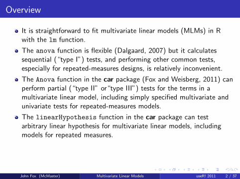
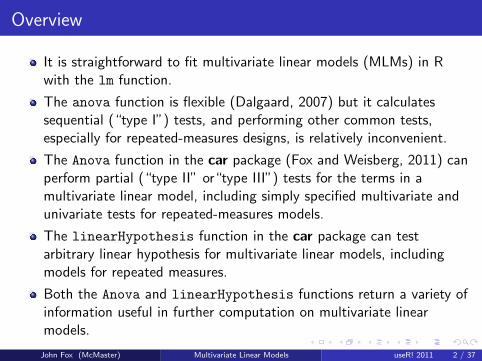
It is straightforward to fit multivariate linear models (MLMs) in Rwith the lm function.
The anova function is flexible (Dalgaard, 2007) but it calculatessequential (“type I”) tests, and performing other common tests,especially for repeated-measures designs, is relatively inconvenient.
The Anova function in the car package (Fox and Weisberg, 2011) canperform partial (“type II” or“type III”) tests for the terms in amultivariate linear model, including simply specified multivariate andunivariate tests for repeated-measures models.
The linearHypothesis function in the car package can testarbitrary linear hypothesis for multivariate linear models, includingmodels for repeated measures.
Both the Anova and linearHypothesis functions return a variety ofinformation useful in further computation on multivariate linearmodels.
John Fox (McMaster) Multivariate Linear Models useR! 2011 2 / 37
Overview
It is straightforward to fit multivariate linear models (MLMs) in Rwith the lm function.
The anova function is flexible (Dalgaard, 2007) but it calculatessequential (“type I”) tests, and performing other common tests,especially for repeated-measures designs, is relatively inconvenient.
The Anova function in the car package (Fox and Weisberg, 2011) canperform partial (“type II” or“type III”) tests for the terms in amultivariate linear model, including simply specified multivariate andunivariate tests for repeated-measures models.
The linearHypothesis function in the car package can testarbitrary linear hypothesis for multivariate linear models, includingmodels for repeated measures.
Both the Anova and linearHypothesis functions return a variety ofinformation useful in further computation on multivariate linearmodels.
John Fox (McMaster) Multivariate Linear Models useR! 2011 2 / 37
A Simple Example: The Anderson-Fisher Iris Data
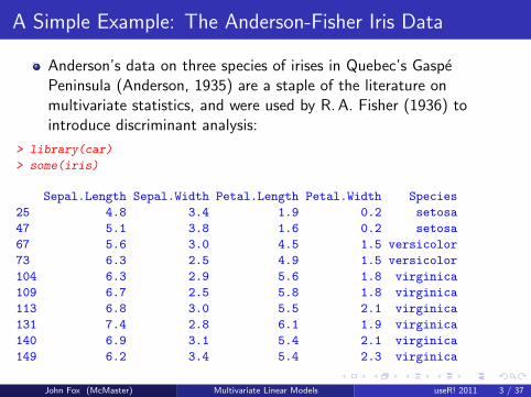
Anderson’s data on three species of irises in Quebec’s GaspePeninsula (Anderson, 1935) are a staple of the literature onmultivariate statistics, and were used by R. A. Fisher (1936) tointroduce discriminant analysis:
> library(car)
> some(iris)
Sepal.Length Sepal.Width Petal.Length Petal.Width Species
25 4.8 3.4 1.9 0.2 setosa
47 5.1 3.8 1.6 0.2 setosa
67 5.6 3.0 4.5 1.5 versicolor
73 6.3 2.5 4.9 1.5 versicolor
104 6.3 2.9 5.6 1.8 virginica
109 6.7 2.5 5.8 1.8 virginica
113 6.8 3.0 5.5 2.1 virginica
131 7.4 2.8 6.1 1.9 virginica
140 6.9 3.1 5.4 2.1 virginica
149 6.2 3.4 5.4 2.3 virginica
John Fox (McMaster) Multivariate Linear Models useR! 2011 3 / 37
A Simple Example: The Anderson-Fisher Iris Data
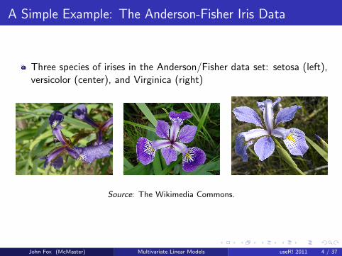
Three species of irises in the Anderson/Fisher data set: setosa (left),versicolor (center), and Virginica (right)
Source: The Wikimedia Commons.
John Fox (McMaster) Multivariate Linear Models useR! 2011 4 / 37
A Simple Example: The Anderson-Fisher Iris Data
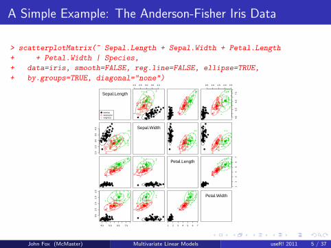
> scatterplotMatrix(~ Sepal.Length + Sepal.Width + Petal.Length
+ + Petal.Width | Species,
+ data=iris, smooth=FALSE, reg.line=FALSE, ellipse=TRUE,
+ by.groups=TRUE, diagonal="none")
● setosaversicolorvirginica
Sepal.Length
2.0 2.5 3.0 3.5 4.0
●●
●●
●
●
●
●
●
●
●
●●
●
●●
●
●
●
●
●
●
●
●
●● ●
●●
●●
●●
●
●●
●
●
●
●●
●●
●●
●
●
●
●
●●●
●●
●●
●●
●●
●
●
●
●
●
●
●
●●
●
●●
●
●
●
●
●
●
●
●
●●●
●●
●●
●●
●
●●
●
●
●
●●
●●
●●
●
●
●
●
●●●
●●
●●
0.5 1.0 1.5 2.0 2.5
4.5
5.5
6.5
7.5
●●●●
●
●
●
●
●
●
●
●●
●
●●
●
●
●
●
●
●
●
●
●● ●●●
●●
●●
●
●●
●
●
●
●●
●●
●●
●
●
●
●
●●●
●●
●●
2.0
2.5
3.0
3.5
4.0
●
●
●●
●
●
● ●
●
●
●
●
●●
●
●
●
●
●●
●
●●
●●
●
●●●
●●
●
●●
●●
●●
●
●●
●
●
●
●
●
●
●
●
●●●
●●●●
Sepal.Width●
●
●●
●
●
●●
●
●
●
●
●●
●
●
●
●
●●
●
●●
●●
●
●●
●
●●
●
●●
●●
●●
●
●●
●
●
●
●
●
●
●
●
●●●
●●●●
●
●
●●
●
●
●●
●
●
●
●
●●
●
●
●
●
●●
●
●●
●●
●
●●●
●●
●
●●
●●
●●
●
●●
●
●
●
●
●
●
●
●
●●●
●●●●
●●●● ●
●● ●● ● ●●
●● ●
●●●
●●
●●
●
●●
●● ●●●● ●● ●●
● ●●●●
●●●●
●
●●
● ●●●●
●●
●●
●● ●● ●
●●●● ● ●●
●● ●
●●●
●●
●●
●
●●
● ●●●●● ● ●●●● ●●●
●●● ●●
●
●●
● ●●●●
●●
●●
Petal.Length
12
34
56
7
●●●●●
●●●●●●●●
●●●●●
●●
●●
●
●●● ●●●●● ●●●●●●
●●●
●●●●
●
●●●●●●●
●●
●●
4.5 5.5 6.5 7.5
0.5
1.0
1.5
2.0
2.5
●●●● ●
●●
●●●
●●●●
●
●●● ●●
●
●
●
●
● ●
●
●●●●
●
●●●● ●
●● ●
●●●
●
●●
●● ●●●●
●●
●●
●● ●● ●
●●●●
●●●
●●●
●●● ●●
●
●
●
●
●●
●
●●●●
●
●●●● ●
●● ●
●●●
●
●●
●● ●●●●
●●
●●
1 2 3 4 5 6 7
●●●●●
●●●●●●●
●●●
●●● ●●
●
●
●
●
●●
●
●●●●
●
●●●●●●
●●●●●
●
●●
●●●●●●
●●
●● Petal.Width
John Fox (McMaster) Multivariate Linear Models useR! 2011 5 / 37
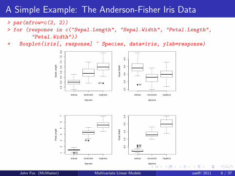
A Simple Example: The Anderson-Fisher Iris Data> par(mfrow=c(2, 2))
> for (response in c("Sepal.Length", "Sepal.Width", "Petal.Length",
"Petal.Width"))
+ Boxplot(iris[, response] ~ Species, data=iris, ylab=response)
●
setosa versicolor virginica
4.5
5.0
5.5
6.0
6.5
7.0
7.5
8.0
Species
Sep
al.L
engt
h
107●
setosa versicolor virginica
2.0
2.5
3.0
3.5
4.0
Species
Sep
al.W
idth
42
●
●
setosa versicolor virginica
12
34
56
7
Species
Pet
al.L
engt
h
23
99
●
●
setosa versicolor virginica
0.5
1.0
1.5
2.0
2.5
Species
Pet
al.W
idth
2444
John Fox (McMaster) Multivariate Linear Models useR! 2011 6 / 37
A Simple Example: The Anderson-Fisher Iris Data
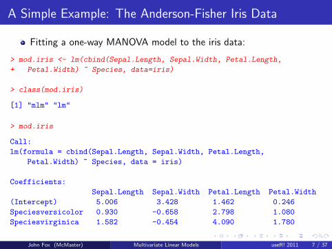
Fitting a one-way MANOVA model to the iris data:
> mod.iris <- lm(cbind(Sepal.Length, Sepal.Width, Petal.Length,
+ Petal.Width) ~ Species, data=iris)
> class(mod.iris)
[1] "mlm" "lm"
> mod.iris
Call:
lm(formula = cbind(Sepal.Length, Sepal.Width, Petal.Length,
Petal.Width) ~ Species, data = iris)
Coefficients:
Sepal.Length Sepal.Width Petal.Length Petal.Width
(Intercept) 5.006 3.428 1.462 0.246
Speciesversicolor 0.930 -0.658 2.798 1.080
Speciesvirginica 1.582 -0.454 4.090 1.780
John Fox (McMaster) Multivariate Linear Models useR! 2011 7 / 37
A Simple Example: The Anderson-Fisher Iris Data
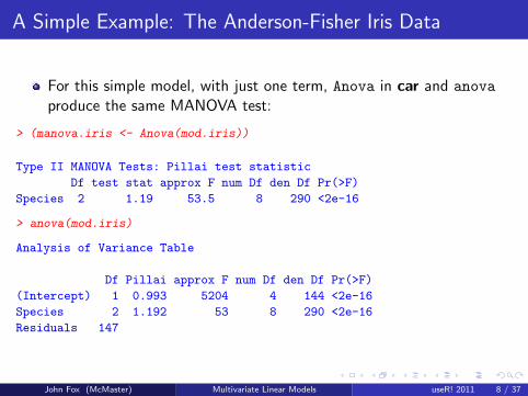
For this simple model, with just one term, Anova in car and anova
produce the same MANOVA test:
> (manova.iris <- Anova(mod.iris))
Type II MANOVA Tests: Pillai test statistic
Df test stat approx F num Df den Df Pr(>F)
Species 2 1.19 53.5 8 290 <2e-16
> anova(mod.iris)
Analysis of Variance Table
Df Pillai approx F num Df den Df Pr(>F)
(Intercept) 1 0.993 5204 4 144 <2e-16
Species 2 1.192 53 8 290 <2e-16
Residuals 147
John Fox (McMaster) Multivariate Linear Models useR! 2011 8 / 37
A Simple Example: The Anderson-Fisher Iris Data
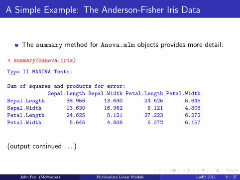
The summary method for Anova.mlm objects provides more detail:
> summary(manova.iris)
Type II MANOVA Tests:
Sum of squares and products for error:
Sepal.Length Sepal.Width Petal.Length Petal.Width
Sepal.Length 38.956 13.630 24.625 5.645
Sepal.Width 13.630 16.962 8.121 4.808
Petal.Length 24.625 8.121 27.223 6.272
Petal.Width 5.645 4.808 6.272 6.157
(output continued . . . )
John Fox (McMaster) Multivariate Linear Models useR! 2011 9 / 37
A Simple Example: The Anderson-Fisher Iris Data
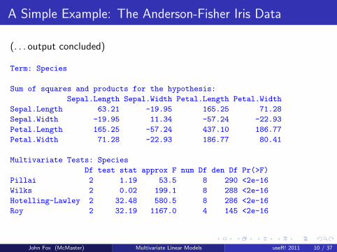
(. . . output concluded)
Term: Species
Sum of squares and products for the hypothesis:
Sepal.Length Sepal.Width Petal.Length Petal.Width
Sepal.Length 63.21 -19.95 165.25 71.28
Sepal.Width -19.95 11.34 -57.24 -22.93
Petal.Length 165.25 -57.24 437.10 186.77
Petal.Width 71.28 -22.93 186.77 80.41
Multivariate Tests: Species
Df test stat approx F num Df den Df Pr(>F)
Pillai 2 1.19 53.5 8 290 <2e-16
Wilks 2 0.02 199.1 8 288 <2e-16
Hotelling-Lawley 2 32.48 580.5 8 286 <2e-16
Roy 2 32.19 1167.0 4 145 <2e-16
John Fox (McMaster) Multivariate Linear Models useR! 2011 10 / 37
A Simple Example: The Anderson-Fisher Iris Data
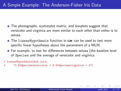
The photographs, scatterplot matrix, and boxplots suggest thatversicolor and virginica are more similar to each other than either is tosetosa.
The linearHypothesis function in car can be used to test morespecific linear hypotheses about the parameters of a MLM.
For example, to test for differences between setosa (the baseline levelof Species and the average of versicolor and virginica:
> linearHypothesis(mod.iris,
+ "0.5*Speciesversicolor + 0.5*Speciesvirginica = 0")
John Fox (McMaster) Multivariate Linear Models useR! 2011 11 / 37
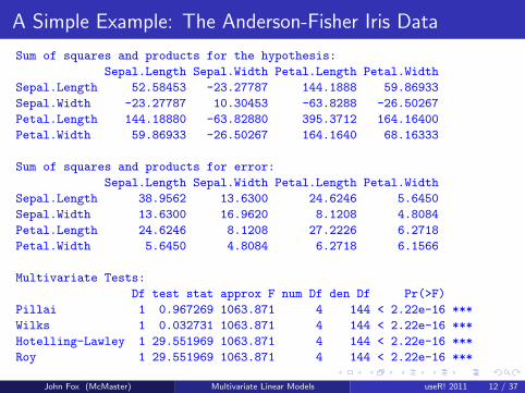
A Simple Example: The Anderson-Fisher Iris Data
Sum of squares and products for the hypothesis:
Sepal.Length Sepal.Width Petal.Length Petal.Width
Sepal.Length 52.58453 -23.27787 144.1888 59.86933
Sepal.Width -23.27787 10.30453 -63.8288 -26.50267
Petal.Length 144.18880 -63.82880 395.3712 164.16400
Petal.Width 59.86933 -26.50267 164.1640 68.16333
Sum of squares and products for error:
Sepal.Length Sepal.Width Petal.Length Petal.Width
Sepal.Length 38.9562 13.6300 24.6246 5.6450
Sepal.Width 13.6300 16.9620 8.1208 4.8084
Petal.Length 24.6246 8.1208 27.2226 6.2718
Petal.Width 5.6450 4.8084 6.2718 6.1566
Multivariate Tests:
Df test stat approx F num Df den Df Pr(>F)
Pillai 1 0.967269 1063.871 4 144 < 2.22e-16 ***
Wilks 1 0.032731 1063.871 4 144 < 2.22e-16 ***
Hotelling-Lawley 1 29.551969 1063.871 4 144 < 2.22e-16 ***
Roy 1 29.551969 1063.871 4 144 < 2.22e-16 ***
John Fox (McMaster) Multivariate Linear Models useR! 2011 12 / 37
A Simple Example: The Anderson-Fisher Iris Data
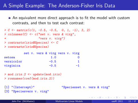
An equivalent more direct approach is to fit the model with customcontrasts, and then to test each contrast:
> C <- matrix(c(1, -0.5, -0.5, 0, 1, -1), 3, 2)
> colnames(C) <- c("set v. vers & virg",
+ "vers v. virg")
> contrasts(iris$Species) <- C
> contrasts(iris$Species)
set v. vers & virg vers v. virg
setosa 1.0 0
versicolor -0.5 1
virginica -0.5 -1
> mod.iris.2 <- update(mod.iris)
> rownames(coef(mod.iris.2))
[1] "(Intercept)" "Speciesset v. vers & virg"
[3] "Speciesvers v. virg"
John Fox (McMaster) Multivariate Linear Models useR! 2011 13 / 37
A Simple Example: The Anderson-Fisher Iris Data
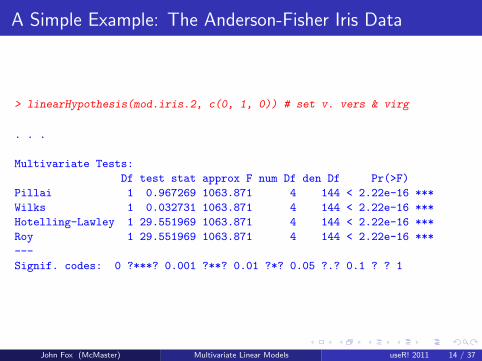
> linearHypothesis(mod.iris.2, c(0, 1, 0)) # set v. vers & virg
. . .
Multivariate Tests:
Df test stat approx F num Df den Df Pr(>F)
Pillai 1 0.967269 1063.871 4 144 < 2.22e-16 ***
Wilks 1 0.032731 1063.871 4 144 < 2.22e-16 ***
Hotelling-Lawley 1 29.551969 1063.871 4 144 < 2.22e-16 ***
Roy 1 29.551969 1063.871 4 144 < 2.22e-16 ***
---
Signif. codes: 0 ?***? 0.001 ?**? 0.01 ?*? 0.05 ?.? 0.1 ? ? 1
John Fox (McMaster) Multivariate Linear Models useR! 2011 14 / 37
Handling Repeated Measures
Repeated-measures data arise when multivariate responses representthe same individuals measured on a response variable (or variables) ondifferent occasions or under different circumstances.
There may be a more or less complex design on the repeatedmeasures.
The simplest case is that of a single repeated-measures orwithin-subjects factor.
John Fox (McMaster) Multivariate Linear Models useR! 2011 15 / 37
Handling Repeated Measures
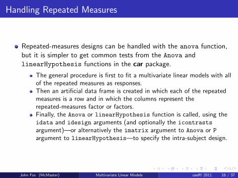
Repeated-measures designs can be handled with the anova function,but it is simpler to get common tests from the Anova andlinearHypothesis functions in the car package.
The general procedure is first to fit a multivariate linear models with allof the repeated measures as responses.Then an artificial data frame is created in which each of the repeatedmeasures is a row and in which the columns represent therepeated-measures factor or factors.Finally, the Anova or linearHypothesis function is called, using theidata and idesign arguments (and optionally the icontrasts
argument)—or alternatively the imatrix argument to Anova or Pargument to linearHypothesis—to specify the intra-subject design.
John Fox (McMaster) Multivariate Linear Models useR! 2011 16 / 37
Handling Repeated Measures
Repeated-measures designs can be handled with the anova function,but it is simpler to get common tests from the Anova andlinearHypothesis functions in the car package.
The general procedure is first to fit a multivariate linear models with allof the repeated measures as responses.
Then an artificial data frame is created in which each of the repeatedmeasures is a row and in which the columns represent therepeated-measures factor or factors.Finally, the Anova or linearHypothesis function is called, using theidata and idesign arguments (and optionally the icontrasts
argument)—or alternatively the imatrix argument to Anova or Pargument to linearHypothesis—to specify the intra-subject design.
John Fox (McMaster) Multivariate Linear Models useR! 2011 16 / 37
Handling Repeated Measures
Repeated-measures designs can be handled with the anova function,but it is simpler to get common tests from the Anova andlinearHypothesis functions in the car package.
The general procedure is first to fit a multivariate linear models with allof the repeated measures as responses.Then an artificial data frame is created in which each of the repeatedmeasures is a row and in which the columns represent therepeated-measures factor or factors.
Finally, the Anova or linearHypothesis function is called, using theidata and idesign arguments (and optionally the icontrasts
argument)—or alternatively the imatrix argument to Anova or Pargument to linearHypothesis—to specify the intra-subject design.
John Fox (McMaster) Multivariate Linear Models useR! 2011 16 / 37
Handling Repeated Measures
Repeated-measures designs can be handled with the anova function,but it is simpler to get common tests from the Anova andlinearHypothesis functions in the car package.
The general procedure is first to fit a multivariate linear models with allof the repeated measures as responses.Then an artificial data frame is created in which each of the repeatedmeasures is a row and in which the columns represent therepeated-measures factor or factors.Finally, the Anova or linearHypothesis function is called, using theidata and idesign arguments (and optionally the icontrasts
argument)—or alternatively the imatrix argument to Anova or Pargument to linearHypothesis—to specify the intra-subject design.
John Fox (McMaster) Multivariate Linear Models useR! 2011 16 / 37
Handling Repeated Measures
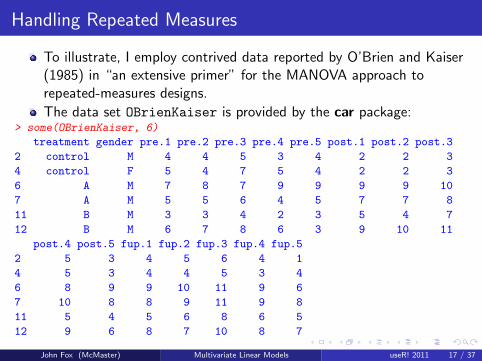
To illustrate, I employ contrived data reported by O’Brien and Kaiser(1985) in “an extensive primer” for the MANOVA approach torepeated-measures designs.
The data set OBrienKaiser is provided by the car package:> some(OBrienKaiser, 6)
treatment gender pre.1 pre.2 pre.3 pre.4 pre.5 post.1 post.2 post.3
2 control M 4 4 5 3 4 2 2 3
4 control F 5 4 7 5 4 2 2 3
6 A M 7 8 7 9 9 9 9 10
7 A M 5 5 6 4 5 7 7 8
11 B M 3 3 4 2 3 5 4 7
12 B M 6 7 8 6 3 9 10 11
post.4 post.5 fup.1 fup.2 fup.3 fup.4 fup.5
2 5 3 4 5 6 4 1
4 5 3 4 4 5 3 4
6 8 9 9 10 11 9 6
7 10 8 8 9 11 9 8
11 5 4 5 6 8 6 5
12 9 6 8 7 10 8 7
John Fox (McMaster) Multivariate Linear Models useR! 2011 17 / 37
Handling Repeated Measures
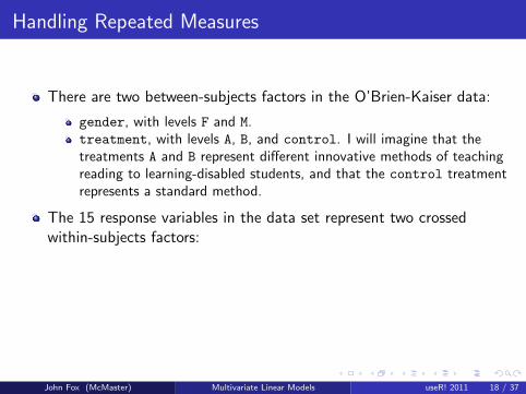
There are two between-subjects factors in the O’Brien-Kaiser data:
gender, with levels F and M.treatment, with levels A, B, and control. I will imagine that thetreatments A and B represent different innovative methods of teachingreading to learning-disabled students, and that the control treatmentrepresents a standard method.
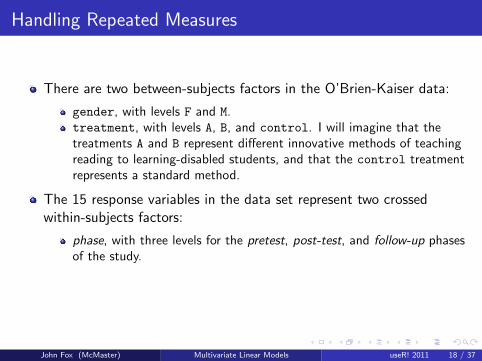
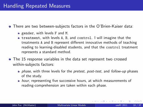
The 15 response variables in the data set represent two crossedwithin-subjects factors:
phase, with three levels for the pretest, post-test, and follow-up phasesof the study.hour, representing five successive hours, at which measurements ofreading-comprehension are taken within each phase.
John Fox (McMaster) Multivariate Linear Models useR! 2011 18 / 37
Handling Repeated Measures
There are two between-subjects factors in the O’Brien-Kaiser data:
gender, with levels F and M.
treatment, with levels A, B, and control. I will imagine that thetreatments A and B represent different innovative methods of teachingreading to learning-disabled students, and that the control treatmentrepresents a standard method.
The 15 response variables in the data set represent two crossedwithin-subjects factors:
phase, with three levels for the pretest, post-test, and follow-up phasesof the study.hour, representing five successive hours, at which measurements ofreading-comprehension are taken within each phase.
John Fox (McMaster) Multivariate Linear Models useR! 2011 18 / 37

Handling Repeated Measures
There are two between-subjects factors in the O’Brien-Kaiser data:
gender, with levels F and M.treatment, with levels A, B, and control. I will imagine that thetreatments A and B represent different innovative methods of teachingreading to learning-disabled students, and that the control treatmentrepresents a standard method.
The 15 response variables in the data set represent two crossedwithin-subjects factors:
phase, with three levels for the pretest, post-test, and follow-up phasesof the study.hour, representing five successive hours, at which measurements ofreading-comprehension are taken within each phase.
John Fox (McMaster) Multivariate Linear Models useR! 2011 18 / 37
Handling Repeated Measures
There are two between-subjects factors in the O’Brien-Kaiser data:
gender, with levels F and M.treatment, with levels A, B, and control. I will imagine that thetreatments A and B represent different innovative methods of teachingreading to learning-disabled students, and that the control treatmentrepresents a standard method.
The 15 response variables in the data set represent two crossedwithin-subjects factors:
phase, with three levels for the pretest, post-test, and follow-up phasesof the study.
hour, representing five successive hours, at which measurements ofreading-comprehension are taken within each phase.
John Fox (McMaster) Multivariate Linear Models useR! 2011 18 / 37
Handling Repeated Measures
There are two between-subjects factors in the O’Brien-Kaiser data:
gender, with levels F and M.treatment, with levels A, B, and control. I will imagine that thetreatments A and B represent different innovative methods of teachingreading to learning-disabled students, and that the control treatmentrepresents a standard method.
The 15 response variables in the data set represent two crossedwithin-subjects factors:
phase, with three levels for the pretest, post-test, and follow-up phasesof the study.hour, representing five successive hours, at which measurements ofreading-comprehension are taken within each phase.
John Fox (McMaster) Multivariate Linear Models useR! 2011 18 / 37
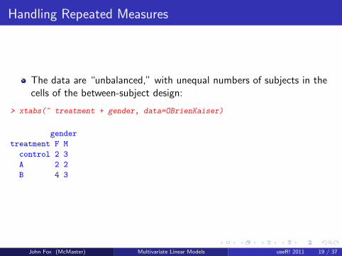
Handling Repeated Measures
The data are “unbalanced,” with unequal numbers of subjects in thecells of the between-subject design:
> xtabs(~ treatment + gender, data=OBrienKaiser)
gender
treatment F M
control 2 3
A 2 2
B 4 3
John Fox (McMaster) Multivariate Linear Models useR! 2011 19 / 37
Handling Repeated Measures
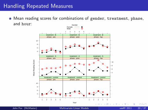
Mean reading scores for combinations of gender, treatment, phase,and hour:
hour
Mea
n R
eadi
ng S
core
4
6
8
10
1 2 3 4 5
●●
●● ●
: phase pre : treatment control
● ●
●●
●
: phase post : treatment control
1 2 3 4 5
● ●●
●
●
: phase fup : treatment control
●● ● ●
●
: phase pre : treatment A
● ●● ●
●
: phase post : treatment A
4
6
8
10
●●
●
●
●
: phase fup : treatment A
4
6
8
10
● ●●
● ●
: phase pre : treatment B
1 2 3 4 5
● ●●
●
●
: phase post : treatment B
● ●
●
● ●
: phase fup : treatment B
GenderFemaleMale ●
John Fox (McMaster) Multivariate Linear Models useR! 2011 20 / 37
Handling Repeated Measures
It appears as if reading improves across phases in the twoexperimental treatments but not in the control group, suggesting apossible treatment-by-phase interaction.
There is a possibly quadratic relationship of reading to hour withineach phase, with an initial rise and then decline, perhaps representingfatigue, suggesting an hour main effect.
Males and females respond similarly to the control and B treatmentgroups, but that males do better than females in the A treatmentgroup, suggesting a possible gender-by-treatment interaction.
John Fox (McMaster) Multivariate Linear Models useR! 2011 21 / 37
Handling Repeated Measures
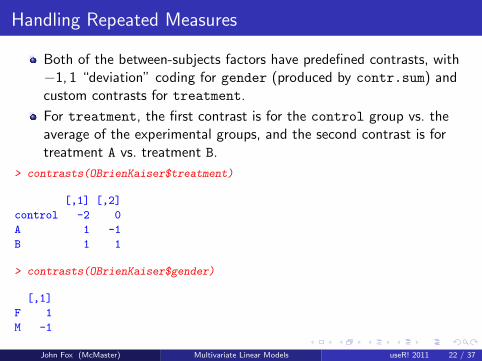
Both of the between-subjects factors have predefined contrasts, with−1, 1 “deviation” coding for gender (produced by contr.sum) andcustom contrasts for treatment.
For treatment, the first contrast is for the control group vs. theaverage of the experimental groups, and the second contrast is fortreatment A vs. treatment B.
> contrasts(OBrienKaiser$treatment)
[,1] [,2]
control -2 0
A 1 -1
B 1 1
> contrasts(OBrienKaiser$gender)
[,1]
F 1
M -1
John Fox (McMaster) Multivariate Linear Models useR! 2011 22 / 37
Handling Repeated Measures
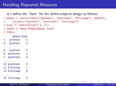
I define the “data” for the within-subjects design as follows:> phase <- factor(rep(c("pretest", "posttest", "followup"), each=5),
+ levels=c("pretest", "posttest", "followup"))
> hour <- ordered(rep(1:5, 3))
> idata <- data.frame(phase, hour)
> idata
phase hour
1 pretest 1
2 pretest 2
. . .
5 pretest 5
6 posttest 1
7 posttest 2
. . .
10 posttest 5
11 followup 1
12 followup 2
. . .
15 followup 5
John Fox (McMaster) Multivariate Linear Models useR! 2011 23 / 37
Handling Repeated Measures
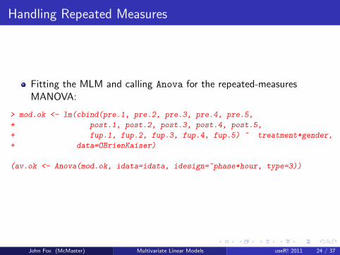
Fitting the MLM and calling Anova for the repeated-measuresMANOVA:
> mod.ok <- lm(cbind(pre.1, pre.2, pre.3, pre.4, pre.5,
+ post.1, post.2, post.3, post.4, post.5,
+ fup.1, fup.2, fup.3, fup.4, fup.5) ~ treatment*gender,
+ data=OBrienKaiser)
(av.ok <- Anova(mod.ok, idata=idata, idesign=~phase*hour, type=3))
John Fox (McMaster) Multivariate Linear Models useR! 2011 24 / 37
Handling Repeated Measures
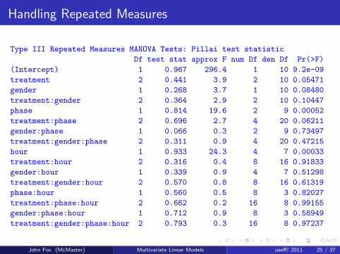
Type III Repeated Measures MANOVA Tests: Pillai test statistic
Df test stat approx F num Df den Df Pr(>F)
(Intercept) 1 0.967 296.4 1 10 9.2e-09
treatment 2 0.441 3.9 2 10 0.05471
gender 1 0.268 3.7 1 10 0.08480
treatment:gender 2 0.364 2.9 2 10 0.10447
phase 1 0.814 19.6 2 9 0.00052
treatment:phase 2 0.696 2.7 4 20 0.06211
gender:phase 1 0.066 0.3 2 9 0.73497
treatment:gender:phase 2 0.311 0.9 4 20 0.47215
hour 1 0.933 24.3 4 7 0.00033
treatment:hour 2 0.316 0.4 8 16 0.91833
gender:hour 1 0.339 0.9 4 7 0.51298
treatment:gender:hour 2 0.570 0.8 8 16 0.61319
phase:hour 1 0.560 0.5 8 3 0.82027
treatment:phase:hour 2 0.662 0.2 16 8 0.99155
gender:phase:hour 1 0.712 0.9 8 3 0.58949
treatment:gender:phase:hour 2 0.793 0.3 16 8 0.97237
John Fox (McMaster) Multivariate Linear Models useR! 2011 25 / 37
Handling Repeated Measures
Following O’Brien and Kaiser, I report type-III tests, which arecomputed correctly because the contrasts employed for treatmentand gender, and hence their interaction, are orthogonal in therow-basis of the between-subjects design.
When the idata and idesign arguments are specified, Anovaautomatically constructs orthogonal contrasts for different terms inthe within-subjects design, using contr.sum for a factor such asphase and contr.poly for an ordered factor such as hour.
Alternatively, the user can assign contrasts to the columns of theintra-subject data, either directly or via the icontrasts argument toAnova. Anova checks that the within-subjects contrast coding fordifferent terms is orthogonal.
John Fox (McMaster) Multivariate Linear Models useR! 2011 26 / 37
Handling Repeated Measures
The results show that the anticipated hour effect is statisticallysignificant.
The treatment × phase and treatment × gender interactions arenot quite significant.
There is, however, a statistically significant phase main effect.
We should not over-interpret these results, partly because the data setis small and partly because it is contrived.
John Fox (McMaster) Multivariate Linear Models useR! 2011 27 / 37
Handling Repeated Measures
The summary method for Anova.mlm objects can report a variety ofinformation, including a traditional “univariate” repeated-measuresANOVA with tests of sphericity and corrections for non-sphericity.
Suppressing the multivariate tests:
John Fox (McMaster) Multivariate Linear Models useR! 2011 28 / 37
Handling Repeated Measures
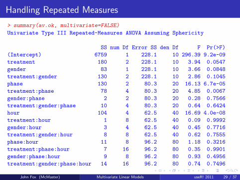
> summary(av.ok, multivariate=FALSE)
Univariate Type III Repeated-Measures ANOVA Assuming Sphericity
SS num Df Error SS den Df F Pr(>F)
(Intercept) 6759 1 228.1 10 296.39 9.2e-09
treatment 180 2 228.1 10 3.94 0.0547
gender 83 1 228.1 10 3.66 0.0848
treatment:gender 130 2 228.1 10 2.86 0.1045
phase 130 2 80.3 20 16.13 6.7e-05
treatment:phase 78 4 80.3 20 4.85 0.0067
gender:phase 2 2 80.3 20 0.28 0.7566
treatment:gender:phase 10 4 80.3 20 0.64 0.6424
hour 104 4 62.5 40 16.69 4.0e-08
treatment:hour 1 8 62.5 40 0.09 0.9992
gender:hour 3 4 62.5 40 0.45 0.7716
treatment:gender:hour 8 8 62.5 40 0.62 0.7555
phase:hour 11 8 96.2 80 1.18 0.3216
treatment:phase:hour 7 16 96.2 80 0.35 0.9901
gender:phase:hour 9 8 96.2 80 0.93 0.4956
treatment:gender:phase:hour 14 16 96.2 80 0.74 0.7496
John Fox (McMaster) Multivariate Linear Models useR! 2011 29 / 37
Handling Repeated Measures
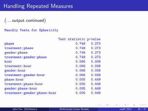
(. . . output continued)
Mauchly Tests for Sphericity
Test statistic p-value
phase 0.749 0.273
treatment:phase 0.749 0.273
gender:phase 0.749 0.273
treatment:gender:phase 0.749 0.273
hour 0.066 0.008
treatment:hour 0.066 0.008
gender:hour 0.066 0.008
treatment:gender:hour 0.066 0.008
phase:hour 0.005 0.449
treatment:phase:hour 0.005 0.449
gender:phase:hour 0.005 0.449
treatment:gender:phase:hour 0.005 0.449
John Fox (McMaster) Multivariate Linear Models useR! 2011 30 / 37
Handling Repeated Measures
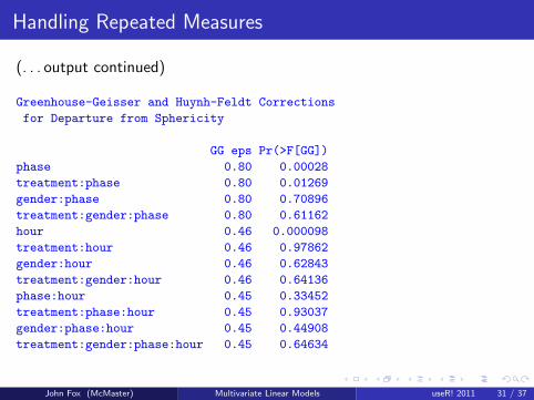
(. . . output continued)
Greenhouse-Geisser and Huynh-Feldt Corrections
for Departure from Sphericity
GG eps Pr(>F[GG])
phase 0.80 0.00028
treatment:phase 0.80 0.01269
gender:phase 0.80 0.70896
treatment:gender:phase 0.80 0.61162
hour 0.46 0.000098
treatment:hour 0.46 0.97862
gender:hour 0.46 0.62843
treatment:gender:hour 0.46 0.64136
phase:hour 0.45 0.33452
treatment:phase:hour 0.45 0.93037
gender:phase:hour 0.45 0.44908
treatment:gender:phase:hour 0.45 0.64634
John Fox (McMaster) Multivariate Linear Models useR! 2011 31 / 37
Handling Repeated Measures
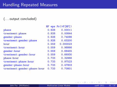
(. . . output concluded)
HF eps Pr(>F[HF])
phase 0.928 0.00011
treatment:phase 0.928 0.00844
gender:phase 0.928 0.74086
treatment:gender:phase 0.928 0.63200
hour 0.559 0.000023
treatment:hour 0.559 0.98866
gender:hour 0.559 0.66455
treatment:gender:hour 0.559 0.66930
phase:hour 0.733 0.32966
treatment:phase:hour 0.733 0.97523
gender:phase:hour 0.733 0.47803
treatment:gender:phase:hour 0.733 0.70801
John Fox (McMaster) Multivariate Linear Models useR! 2011 32 / 37
Handling Repeated Measures
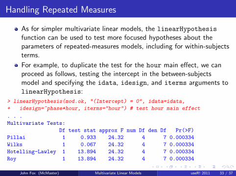
As for simpler multivariate linear models, the linearHypothesis
function can be used to test more focused hypotheses about theparameters of repeated-measures models, including for within-subjectsterms.
For example, to duplicate the test for the hour main effect, we canproceed as follows, testing the intercept in the between-subjectsmodel and specifying the idata, idesign, and iterms arguments tolinearHypothesis:
> linearHypothesis(mod.ok, "(Intercept) = 0", idata=idata,
+ idesign=~phase*hour, iterms="hour") # test hour main effect
. . .
Multivariate Tests:
Df test stat approx F num Df den Df Pr(>F)
Pillai 1 0.933 24.32 4 7 0.000334
Wilks 1 0.067 24.32 4 7 0.000334
Hotelling-Lawley 1 13.894 24.32 4 7 0.000334
Roy 1 13.894 24.32 4 7 0.000334
John Fox (McMaster) Multivariate Linear Models useR! 2011 33 / 37
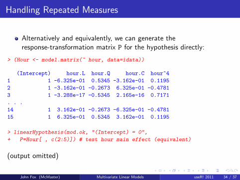
Handling Repeated Measures
Alternatively and equivalently, we can generate theresponse-transformation matrix P for the hypothesis directly:
> (Hour <- model.matrix(~ hour, data=idata))
(Intercept) hour.L hour.Q hour.C hour^4
1 1 -6.325e-01 0.5345 -3.162e-01 0.1195
2 1 -3.162e-01 -0.2673 6.325e-01 -0.4781
3 1 -3.288e-17 -0.5345 2.165e-16 0.7171
. . .
14 1 3.162e-01 -0.2673 -6.325e-01 -0.4781
15 1 6.325e-01 0.5345 3.162e-01 0.1195
> linearHypothesis(mod.ok, "(Intercept) = 0",
+ P=Hour[ , c(2:5)]) # test hour main effect (equivalent)
(output omitted)
John Fox (McMaster) Multivariate Linear Models useR! 2011 34 / 37
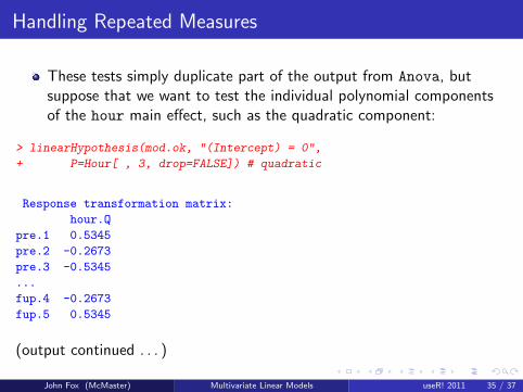
Handling Repeated Measures
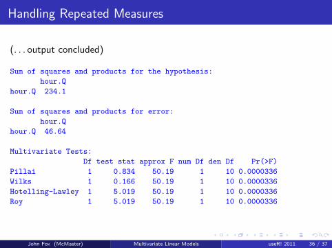
These tests simply duplicate part of the output from Anova, butsuppose that we want to test the individual polynomial componentsof the hour main effect, such as the quadratic component:
> linearHypothesis(mod.ok, "(Intercept) = 0",
+ P=Hour[ , 3, drop=FALSE]) # quadratic
Response transformation matrix:
hour.Q
pre.1 0.5345
pre.2 -0.2673
pre.3 -0.5345
...
fup.4 -0.2673
fup.5 0.5345
(output continued . . . )
John Fox (McMaster) Multivariate Linear Models useR! 2011 35 / 37
Handling Repeated Measures
(. . . output concluded)
Sum of squares and products for the hypothesis:
hour.Q
hour.Q 234.1
Sum of squares and products for error:
hour.Q
hour.Q 46.64
Multivariate Tests:
Df test stat approx F num Df den Df Pr(>F)
Pillai 1 0.834 50.19 1 10 0.0000336
Wilks 1 0.166 50.19 1 10 0.0000336
Hotelling-Lawley 1 5.019 50.19 1 10 0.0000336
Roy 1 5.019 50.19 1 10 0.0000336
John Fox (McMaster) Multivariate Linear Models useR! 2011 36 / 37
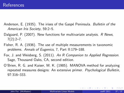
References
Anderson, E. (1935). The irises of the Gaspe Peninsula. Bulletin of theAmerican Iris Society, 59:2–5.
Dalgaard, P. (2007). New functions for multivariate analysis. R News,7(2):2–7.
Fisher, R. A. (1936). The use of multiple measurements in taxonomicproblems. Annals of Eugenics, 7, Part II:179–188.
Fox, J. and Weisberg, S. (2011). An R Companion to Applied Regression.Sage, Thousand Oaks, CA, second edition.
O’Brien, R. G. and Kaiser, M. K. (1985). MANOVA method for analyzingrepeated measures designs: An extensive primer. Psychological Bulletin,97:316–333.
John Fox (McMaster) Multivariate Linear Models useR! 2011 37 / 37


![MGARCH[0.7cm] An R Package for Fitting Multivariate GARCH ... · An R Package for Fitting Multivariate GARCH Models ... Schmidbauer / V.S. Tunal o glu ... o glu / A. R oschOPEC News](https://img.pdfslide.us/doc/110x75/5bb578cf09d3f2e1768cee83/mgarch07cm-an-r-package-for-fitting-multivariate-garch-an-r-package-for.jpg)