1

Testing the Pecking Order Theory with Financial Constraints*

HUILI CHANG† and FRANK M. SONG‡

School of Economics and Finance

The University of Hong Kong

This version: June 2014

ABSTRACT

It is claimed that small and high-growth firms’ tendency to issue equity rejects the

pecking order theory since their information asymmetry problem is most severe. This

paper points out two crucial market imperfections ignored by pecking order, namely

credit rationing caused by information asymmetry in the debt market and the frictions

from the supply side of capital, can explain why small and high-growth firms choose

to issue equity. We adopt financial constraints as proxy for the two imperfections, and

empirically demonstrate that once financial constraints are controlled for, pecking

order provides a better description of firms’ financing behaviors. To address the

endogeneity problem, we analyze an exogenous event-addition into the S&P 500

index, and consistent with our prediction, firms are more likely to issue debt after the

relaxation of financial constraints. Finally, we show that financial constraints are

different from the alternative explanation of debt capacity constraints.

JEL classification: G32

Keywords: financial constraints, pecking order, security issue, capital structure

* We appreciate valuable comments from Sreedhar Bharath, Sheridan Titman, Paul Po-Hsuan Hsu, Xianming Zhou, Shenghui Tong, Lewis Tam, Anzhela Knyazeva, Joye Khoo, Chenggang Xu and participants in the Finance brown bag seminar at the University of Hong Kong, 2013 Five Star Forum in Finance in Beijing, EFMA 2013 Annual Conference and 2013 Asia Finance Association Annual Conference. We thank Chenyu Shan for help in data. We are grateful to John Graham and Jay Ritter for generously providing the tax rate and IPO data online. † Email: kellyhlchang@gmail.com. Tel: (852) 6571-5825. ‡ Email: fmsong@econ.hku.hk. Tel: (852) 2857-8507.

1

1. Introduction

The modified pecking order theory proposed by Myers (1984) and Myers and

Majluf (1984) is one of the most important capital structure theories. Assuming that

managers have inside information about firm value and always behave in the interests

of passive existing shareholders, it predicts that when making investment, firms prefer

internal to external finance, and when seeking external funds, firms prefer safe to

risky securities. Safe securities refer to informationally insensitive securities, whose

future values change less when managers’ inside information is revealed. Among the

existing pool of financing instruments, default-risk-free debt is the safest, risky debt

less safe, hybrid securities (such as convertible bonds and preferred stocks) more risky,

whereas external equity is the riskiest. Accordingly, pecking order predicts a negative

correlation between profitability and leverage, a negative price impact of equity issues

and a less negative impact of debt issues, which are confirmed by subsequent papers

(see, for example, Titman and Wessels, 1988; Spiess and Affleck-Graves, 1995;

Eckbo, 1986).

Nevertheless, the validity of pecking order is far from settled. The most

controversial point is that pecking order fails to explain why so many firms issue

equity, small and high-growth firms in particular. Shyam-Sunder and Myers (1999)

(called SSM henceforth) first propose a key test of pecking order and conclude that it

provides a better first-order description for the 157 large and mature firms. But when

expanding the SSM test to a broader sample and a longer period, Frank and Goyal

(2003) find that pecking order works much worse for small and high-growth firms.

Together with Fama and French (2002, 2005), they claim that small and high-growth

firms’ choice of issuing equity refutes pecking order since these firms tend to most

suffer information asymmetry. Subsequent papers including Agca and Mozumdar

(2007) and Lemmon and Zender (2010) (called LZ henceforth) try to incorporate debt

capacity when testing pecking order, but Leary and Roberts (2010) show only when

firms’ debt capacities are specified as functions of a broad list of firm characteristics,

can pecking order be justified.

2

This paper attempts to reconcile the conflicting test results of pecking order from a

new perspective. Different from the traditional demand side, we focus on the supply

side of capital and argue that small and high-growth firms’ tendency to issue equity

mainly reflects financial constraints they face rather than contradicts pecking order.

According to Fama and French (2001), publicly listed firms are increasingly

dominated by small firms with low profitability and strong growth opportunities. To

fund their growth opportunities, these firms have to rely on external finance. Given

their low profitability and usually few tangible assets, they are least favorable to debt

holders. As a last resort, they have to raise funds in the equity market. In other words,

these small and high-growth firms are forced to issue equity because they do not have

access to the debt market. This is consistent with the zero-leverage puzzle

documented by Strebulaev and Yang (2013). They find that the proportion of

zero-leverage firms is monotonically increasing after the 1970s, and on average over

10% of public nonfinancial US firms have zero debt from 1962 to 2009, among which

two thirds do not pay dividends. Recent papers (Bessler et al., 2012; Dang, 2012; and

Devos et al., 2012) further show the reason for non-dividend-paying zero-leverage

firms to never issue debt is that they are financially constrained.

Our interpretation can also be theoretically justified. There are two crucial market

imperfections that give rise to financial constraints but are missing in the pecking

order theory. The first is credit rationing in the debt market. Pecking order only

emphasizes that information asymmetry can cause the underpricing of good firms in

the equity market, but fails to consider that information asymmetry can also have

adverse effects in the debt market. According to Jaffee and Russell (1976) and Stiglitz

and Weiss (1981, 1983), because of information asymmetry, whenever a bank

increases the interest rate charged, the potential borrowers become riskier as higher

interest rate drives safe borrowers out of the market and also induces borrowers to

undertake riskier projects. As a result, increase in interest rate does not proportionally

raise the expected return, and the optimal interest rate that maximizes banks’ profits

will not clear the loanable funds market. There will be excessive demand for loanable

funds, and some firms will be shut out of the debt market. For these firms, the cost of

3

issuing debt is infinite, while the cost of issuing equity is finite, so issuing equity is

the better choice. Several papers have documented that information asymmetry in the

debt market does affect firms’ capital structure. Faulkender and Petersen (2006) first

show that firms with access to the bond market measured by having a debt rating have

higher leverage after controlling for debt demand. Sufi (2009) and Tang (2009) both

show that mitigation in information asymmetry through either the introduction of

bank loan ratings or the refinement of firms’ credit rating increases firms’ debt

financing and leverage. The second market imperfection comes from the supply side

of capital. Pecking order implicitly assumes that the supply side of capital is fully

flexible, and thus the price of a security only depends on the demand side, i.e., firm

fundamentals. Nevertheless, Baker (2009) argues that the supply side of capital is not

perfectly flexible due to investor tastes, limited intermediation and corporate

opportunism, and can to some extent affect firms’ financing choice. The bank lending

channel summarized by Bernanke and Gertler (1995) is a good example that changes

in bank conditions can affect firms’ borrowing, and Leary (2009) provides direct

evidence that changes in bank funding constraints affect bank-dependent firms’

capital structure. In later analysis, we will use financial constraints1 to account for

these two market imperfections. This is because financial constraints are the

interaction outcome of both demand and supply sides of capital and reflect the

difference in costs between internal and external finance. Since we focus on the listed

US firms and all the firms have access to the equity market, financial constraints

mainly measure their differential access to the debt market. Meanwhile, we also

control for information asymmetry in the equity market. More important, the

measures of financial constraints are time-variant, and thus can better capture the

changes in the supply side of capital, which is in contrast with the dummy of bond

rating used in Faulkender and Petersen (2006).

Since there is no commonly accepted measure of financial constraints, we adopt

four frequently used criteria based on prior studies. First, in a similar spirit to Fazzari, 1 According to Lamont et al. (2001), financial constraints refer to frictions that prevent the firms from funding all

desired investment. It may arise because of credit constraints or inability to borrow, inability to issue equity, dependence on bank loans, or illiquidity of assets. Pecking order only considers the inability to issue equity.

4

Hubbard and Petersen (1988) who use dividend ratio, we use the payout ratio

calculated as the ratio of dividends plus repurchases to operating income following

Almeida, Campello and Weisbach (2004). Second, we use the KZ index first proposed

by Lamont et al. (2001) based on empirical results from Kaplan and Zingales (1997).

Third, we use the WW index from Whited and Wu (2006). Finally, as in Li (2011), we

also use the SA index proposed by Hadlock and Pierce (2010). Following the financial

constraints literature, we define firms in top (bottom) three deciles based on each

financial constraints index2 as financially constrained (unconstrained) firms.

The univariate analysis confirms our conjecture that small and high-growth firms

substitute equity for debt due to financial constraints. Compared with debt issuers,

equity issuers are more financially constrained than debt issuers, and constrained

firms are much smaller and have higher market to book ratio. On the other hand,

small firms tend to be financially constrained, constrained firms issue more equity but

less debt, and it is small and high-growth firms that contribute to the significantly

more equity issues and less debt issuers by constrained firms.

To determine to what extent financial constraints cause small and high-growth

firms to predominantly use equity, we employ the logistic and multinomial logistic

regressions. First, to compare with prior studies, we use the logistic regression to

analyze how firms choose between equity and debt. As expected, financial constraints

do affect firms’ choice between equity and debt. Compared with the intermediate

firms, constrained firms are less likely to issue debt while unconstrained firms are

more likely to do so. Consistent with pecking order, firms with less analyst coverage

or more information asymmetry are inclined to issue debt, and this relationship is

stronger when we include financial constraints. Next, we use the multinomial logistic

regression to analyze how firms choose among the four main financing instruments,

including private equity, SEO, bank loan, and public bond. When we do not include

financial constraints, the prediction of pecking order that firms prefer safe to risk

securities is only weakly supported. Firms followed by more analysts are more likely 2 Here we assume that firms are ranked by their likelihood of being financially constrained. It means that we rank

firms in a reverse order in terms of the payout ratio, and in the sequential order with the KZ index, WW index and SA index.

5

to issue private equity, but only marginally less likely to borrow bank loan. After we

include financial constraints, firms with more analyst coverage are significantly less

likely to borrow bank loan. Furthermore, constrained firms are less likely to issue debt,

and are more likely to issue private equity.

To address the endogeneity problem, we use the addition into the S&P 500 index as

an exogenous event. Since the addition into the S&P 500 index is usually initiated by

the removal of an included firm, and the candidate replacement pool of S&P 500 is

kept confidential, the newly added firm can never predict whether or when it will be

included in the S&P 500, and thus is impossible to adjust its financing choice

beforehand. On the other hand, addition into the S&P 500 can convey information to

the market (Jain, 1987; Dhillon and Johnson, 1991; Denis, Mcconnell, Ovtchinnikov,

and Yu, 2003; Chen, Noronha, and Singal, 2004), certify the quality of firm (Jain,

1987), and enhance investor awareness (Chen, Noronha, and Singal, 2004), which

makes financial institutions or investors more willing to lend to the firm and hence

relax the firm’s financial constraints. We first identify a matching firm for each newly

added firm based on industry, firm size and market to book ratio, and then use the

difference-in-difference method to compare their financing choices three year before

and after the addition. We indeed find that addition into the S&P 500 can relax firms’

financial constraints and firms make more use of debt to raise external funds after the

addition, which suggests that the results found before are not due to omitted variables

or reverse causality.

Finally, to rule out alternative explanations, in particular debt capacity constraints

proposed by LZ, we rerun the SSM test and the LZ modified regression on our sample.

First of all, both regressions confirm our findings that unconstrained firms tend to

follow pecking order while constrained firms do not. More important, the negative

coefficient of the squared financing deficit term for unconstrained firms shows that

financial constraints are different from debt capacity constraints. According to LZ, a

negative coefficient means a higher likelihood of suffering debt capacity constraints.

If financial constraints only measure the debt capacity constraints, unconstrained

firms are supposed to have a high debt capacity and thus should have an insignificant

6

coefficient.

This paper contributes to the literature in several aspects. First, it demonstrates that

the credit rationing in the debt market and frictions from the supply side of capital can

explain the failure of pecking order. After using financial constraints to account for

these two imperfections, we show that firms’ financing behaviors are more consistent

with pecking order. Second, we directly use the new security issue data to test pecking

order, which has several advantages. Since pecking order predicts firms’ incremental

financing choice, new security data enables us to focus on firms’ financing choice

rather than the cumulative leverage. Next, as pointed out by Graham (2000), the

Compustat issue variables cannot provide pure debt versus equity measures, and we

indeed find significant differences between security issuances inferred from the

Compustat issue variables and the actual issuances, which highlights the necessity of

using new security issue data. More important, the availability of bank loan data in

Dealscan makes our sample comprehensive, which is crucial because bank loan is the

dominant external financing source according to Gorton and Winton (2003). Third,

financial constraints can also explain why previous studies find that both the trade-off

and pecking order theories are partially true. On one hand, based on Rajan and

Zingales (1995), the trade-off theory usually models the target leverage as a function

of firm size, tangible assets ratio, and profitability and growth opportunities. The

same four core firm characteristics also classify firms into constrained and

unconstrained firms, and as unconstrained firms can issue much more debt than

constrained firms, it seems plausible that firms have target leverage. However, both

categories of firms do not actually adjust to their target leverage, and they only choose

the less costly way to raise external funds. That may explain why the adjustment

speed estimated by prior studies is rather slow. On the other hand, unconstrained firms

always choose to issue debt except when the equity market is so favorable that the

cost of issuing equity is much smaller. Thus pecking order provides a good

description of the financing behaviors for unconstrained firms but not for constrained

firms. Fourth, this paper illustrates the direct channels through which financial

constraints can affect investment. The heavy reliance on the equity market can lead to

7

two severe problems in the investment of constrained firms. The first problem is

underinvestment. Since the cost of issuing equity is much higher than that of issuing

debt, this higher cost of external finance will force constrained firms to forgo some

positive NPV projects. The other problem is higher investment volatility. As the

equity market is highly cyclical, the investment of constrained firms will be affected

and also be highly volatile.

As mentioned before, this paper is closely related to the papers (including Agca and

Mozumdar (2007) and LZ) that incorporate debt capacity when testing pecking order.

While they consider whether firms have high or low debt capacities measured by the

predicted probability of obtaining a bond rating (or access to the public bond market),

we focus on whether the firm has access to the debt market or not, and have shown

that financial constraints incorporate more than debt capacity constraints. This paper

also helps explain why a broad list of firm characteristics should be used to model

debt capacity as in Leary and Roberts (2010) and why this is still consistent with

pecking order.

Also to explain why firms avoid issuing debt, Halov and Heider (2011) use the

adverse selection cost of debt arisen by the uncertainty of risk. However, we suspect

that the uncertainty of risk is highly correlated with firm risk. This can be seen from

their first measure of recent asset volatilities, which is similar to the measures of firm

risk like cash flow volatility and stock return volatility. For the impact of firm risk on

debt issuance, Helwege and Liang (1996) and Bolton and Freixas (2000) both argue

that higher risk decreases firms’ probability of issuing debt. Here we control for firm

risk by using stock return volatility.

This paper belongs to the financial constraints literature. Initiated by Fazzari,

Hubbard and Petersen (1988), a large number of papers have studied the impact of

financial constraints on firm investment (e.g., Fazzari and Petersen (1993), Kashyap

et al. (1994), and Li (2009)). This paper instead focuses on the impact of financial

constraints on firms’ financing choice. Korajczyk and Levy (2003) also link financial

constraints to capital structure, but they focus on the differential effects of

macroeconomic conditions on capital structure of unconstrained and constrained

8

firms.

Finally, this paper is among the tremendous papers that empirically test pecking

order. Helwege and Liang (1996) also use the logistic and multinomial logistic

regressions to study firms’ financing decision, but they only cover the firms listed in

1983. The most recent paper that directly test pecking order is Bharath, Pasquariello,

and Wu (2009). They construct an information asymmetry index based on the

market’s assessment of adverse selection risk, and evaluate the core assumption of

pecking order that information asymmetry determines capital structure decisions.

However, they do not offer any explanation of why some firms fail to follow pecking

order.

This paper is organized as follows. Session 2 describes the data and methodology.

Session 3 analyzes the empirical results. Session 4 concludes.

2. Data and Methodology

2.1 Sample

This paper uses the new security issue data to test pecking order, and the reasons

are as follows. First, pecking order predicts firms prefer debt over equity for the

incremental financing choice, so we should examine how firms choose among

different financing instruments to test it. This is in contrast with the papers that test

different capital structure theories using leverage as dependent variable (like Titman

and Wessels, 1988; Rajan and Zingales, 1995; Frank and Goyal, 2009). Firms’

leverage is a cumulative result, and may reflect the market timing behavior, which is

allowed in a loose version of pecking order. Second, we should obtain the security

type information directly from new issue databases rather than infer the type of

security issued based on the Compustat data. Ever since Hovakimian, Opler, and

Titman (2001), subsequent papers use the Compustat debt/equity issue variables and a

certain percent of total assets as the cutoff point to determine whether a firm has

issued debt/equity or not. But as pointed out by Graham (2000), the Compustat issue

variables cannot provide pure debt versus equity measures. For instance, the equity

9

measure may include preferred stock issues, conversion of debt into common stock,

and the exercise of stock options, which explains why using the Compustat variables

identify much more equity issues than those recorded in the new issue database. We

will show in the univariate analysis that the inference from the Compustat data gives a

quite different picture from what firms have actually issued, and the new security

issue data can provide a more accurate test of pecking order. Third, thanks to the

development of Dealscan, we can obtain the bank loan issue data, which makes it

possible to use the new issue data to test pecking order. This also differentiates our

paper from prior papers on security choice. Taggart (1977) does not use the security

issuance data, while Marsh (1982) and Jung, Kim and Stulz (1996) only use the new

issue data of equity and public bond, not including bank loan. Since bank loan is the

dominant external financing source according to Gorton and Winton (2003), ignoring

it will bias the results of security choice analysis.

Similar to Erel et. al (2012), we use the new issue data of private equity and SEO

from SDC Platinum, bank loan from Dealscan, and corporate bond and Rule 144-A

debt from Mergent Fixed Investment Securities Database. We exclude any kind of

convertible securities and preferred securities, since these securities are hybrids of

both equity and debt, and we want to conduct a clean test of pecking order.

Specifically, for the bank loan data, following Gomes and Phillips (2012), we focus

on the long-term commercial loans and revolving credit lines, and exclude short-term

loans (loans with less than 1 year of maturity), credit lines and other types of records

(e.g., guarantee, fixed-rate bond or CD, etc.). For the corporate bond data, we exclude

the asset-backed, convertible, preferred, private placements, unit deals and foreign

currency denominated records that are not regular public bonds, but keep the Rule

144-A debt data because Gomes and Phillips (2012) find that 144-A debt issues and

public bond issues are similar. The sample period for new issues data is from 1988 to

2008. That is because according to WRDS Overview of Dealscan, bank loan data

recorded in Dealscan is not well populated before 1988, and there are very few

observations after 2008, which may be due to the financial crisis.

We also use the financial statement data from Compustat and stock data from CRSP.

10

Each category of new issues data is first merged with Compustat based on different

available identifiers3, and we exclude the observations with offering amount missing

or equal to zero. We treat the multiple issues of the same security by one firm within

one fiscal year as one observation, because there may be several tranches for one

issuance. For instance, if a firm issues SEO in both the US and global markets, there

will be two records in SDC. Meanwhile, a syndicated loan package in Dealscan

usually has several facilities. Furthermore, we use the I/B/E/S database to obtain the

analyst coverage information.

In the final sample, to minimize the possibility that firms’ issuance activities are not

covered by these new issue databases, we only keep public companies listed in NYSE,

American Exchange and Nasdaq. Because these are large firms usually with large

fund requirements, their new security issues are more likely to be recorded. Consistent

with prior studies, we exclude financial firms (SIC code: 6000-6999) and utilities

(SIC code: 4900-4999), and firms involved in a significant merger/acquisition

(Compustat footnote code AB). We also exclude firms that report format code 5,

which labels Canadian firms, and firms with missing or zero total assets.

2.2 Main Variables and Methodology

To classify firms into constrained and unconstrained firms, we adopt four

commonly used financial constraints measures. The Appendix provides details on

how to construct them. First is the payout ratio calculated as the ratio of dividends

plus repurchases to operating income as in Almeida, Campello and Weisbach (2004).

As raising external funds is costly, it is rational for financially constrained firms to

retain most of their operating incomes and pay out less. Second, we choose the KZ

index first proposed by Lamont et al. (2001) based on the ordered logistic regression

results of Kaplan and Zingales (1997) on the probability of being classified as

financially constrained. Kaplan and Zingales (1997) place the 49 low dividend firms

3

We use 9-digit CUSIP to identify SEO. But for private placements of equity, 9-digit CUSIP is only available for

a small subset of observations, so we use 6-digit CUSIP whenever the 9-digit one is missing. We use the linking table as in Chava and Roberts (2008) to merge Dealscan with Compustat data, and we use 6-digit CUSIP for the corporate bond data as it is the only identifier provided.

11

identified by Fazzari, Hubbard and Petersen (1988) into five different categories from

least likely to most likely being constrained according to the qualitative information in

firms’ annual report or 10-K. The KZ index is a linear combination of cash flow to

capital, dividends to capital, and cash holdings to capital with negative coefficients,

and Tobin’s Q and debt to total capital with positive coefficients. It is larger for firms

with more financial constraints. Third, we calculate the Whited and Wu (2006) index.

It is constructed via generalized method of moments (GMM) estimation of an

investment Euler equation, and is a linear combination of cash flow to total assets,

dividend-paying dummy, long-term debt to total assets, log of total assets, firm’s

3-digit industry sales growth, and firm’s sale growth. Finally, we compute the SA

index proposed by Hadlock and Pierce (2010). They use a similar method to Kaplan

and Zingales (1997), but they cover a broader and more representative sample. They

document that firm size and age are the most reliable predictors of financial

constraints, and propose the SA index as a combination of firm size and age. Here

firm size is computed as the natural log of inflation-adjusted total assets, and firm age

as the number of years the firm has been on Compustat with a non-missing stock price.

After calculating each financial constraints index, we rank firms based on their

financial constraints level each year, and define firms in top (bottom) three deciles as

financially constrained (unconstrained) firms as in the prior literature.

Following Chang, Dasgupta and Hilary (2006), we measure information asymmetry

by the number of analysts as the maximum number of analysts that make annual

earnings forecasts any month over a 12-month period. We also lag the variable for 3

years to avoid endogeneity. The definitions of all the variables can be found in the

Appendix. To limit the effect of outliers, we winsorize all the firm-level continuous

variables at both one percent tails.

, , 1 ,( 1) ( ),i t i t i tP Debt Logit Xβ ε−= = + (1)

To analyze the financing choice, as in Hovakimian, Opler, and Titman (2001), we

exclude the firm-year observations with multiple issues. To compare with previous

studies, we first run a logistic regression to analyze firms’ choice between equity and

12

debt as Equation (1). The dependent variable equals one if firm borrows bank loan or

issues public bond and zero otherwise. For the independent variables, we first use the

number of analysts to measure information asymmetry. Firms covered by less analysts

normally face more information asymmetry and thus tend to prefer debt to equity

according to pecking order. Then we include the unconstrained and constrained

dummies to find out how financial constraints affect firms’ choice between debt and

equity. Finally, we control for the variables4 that are documented to affect firms’

choice between equity and debt (e.g., Hovakimian, Opler, and Titman, 2001; Chang,

Dasgupta and Hilary, 2006), including Firm size, Log of age, Leverage deviation

(market leverage minus target leverage), Three-year mean ROA, and Market-to-book

ratio, Dummy for M/B>1, Dilution dummy, Tangible assets, S&P rating dummy,

Asset growth rate, R&D ratio, R&D dummy, Share turnover, Z-score, and Stock

return volatility. We estimate the target leverage using the partial-adjustment model in

Flannery and Rangan (2006) as shown by Equation (2). Here , 1i tMDR +is the market

leverage, and the lagged X variables include profitability, depreciation, firm size,

M/B ratio, tangible assets, R&D ratio, R&D dummy5, industry median leverage and

S&P rating.

, 1 , , , 1( ) (1 ) ,i t i t i t i tMDR X MDRλβ λ δ+ += + − + (2)

Second, a multinomial logistic regression is employed to examine how firms

choose among private equity, SEO, bank loan and public bond when seeking external

finance. We create a discrete variable issue for the dependent variable: 1 for private

equity, 2 for SEO, 3 for bank loan, and 4 for public bond. Here we use SEO firms as

the base outcome, since all the firms have access to the public equity market while

firms may not have full access to the rest three markets. The independent variables

mainly follow the logistic regression above, except that we use the deciles based on

each financial constraints index to replace the unconstrained and constrained dummies.

4 As in Hovakimian et al. (2001), we also try to include Net operating loss carry forwards, FD3 and the interaction of Loss dummy and FD3 in the regression, but we find they are not significant. Because it reduces the number of observations a great deal to include them, we do not report them in the main results. 5 Here the definition of R&D dummy follows Fama and French (2002), and is a bid different from that in Flannery and Rangan (2006) where it equals one only when a firm does not report R&D expense, but the results are not affected.

13

That’s because constrained firms seldom issue public bond and unconstrained firms

seldom issue private equity, and the coefficients will be inaccurately estimated if the

unconstrained and constrained dummies are used.

,it PO it itD a b DEF e∆ = + + (3)

where .it it it it it it itDEF DIV I W C D E= + +∆ − = ∆ +∆

To illustrate that financial constraints are different from debt capacity, we rerun the

SSM test and the LZ modified regression. As in Equation (3), Shyam-Sunder and

Myers (1999) test the prediction of pecking order that firms should use debt to fund

financing deficit, and propose that there should be a one-by-one change between net

debt issues and financing deficit. The pecking order hypothesis is that 1POb = . Here

we follow Frank and Goyal (2003) in calculating the financing deficit itDEF , which

excludes the item of current portion of long-term debt in Shyam-Sunder and Myers

(1999). We first recode the missing values of labeled variables in Table 8 of Frank and

Goyal (2003) with zero, and then compute financing deficit as the use of financing

(cash dividend plus investments plus change in working capital) minus the internal

financing (internal cash flow). LZ argues that Equation (3) fails to consider the

concern over debt capacity, and suggests adding the squared financing deficit term to

account for the concavity relationship between net debt issues and financing deficit.

To demonstrate that financial constraints reflect things other than debt capacity, we

run Equation (3) for the unconstrained, intermediate, and constrained firms,

respectively.

As Petersen (2009) suggests, we correct the t-statistics by clustering at both the

firm and year levels for the logistic regressions, the SSM test and the LZ modified

regression, and by clustering at the firm level for the multinomial logistic regressions.

3. Empirical Results

3.1 Univariate Analysis

[Insert Table 1 here]

14

Table 1 gives the descriptive summary of firms choosing each financing instrument.

There are 69,411 firm-year observations from 1987 to 2007, approximately 3,300

firms per year. Among them, 1.42% will issue private equity within the next fiscal

year, 4.12% issue SEOs, 20.90% borrow bank loans, and 4.58% issue public bond.

Confirming Gorton and Winton (2003), bank loan is the dominant external financing

source, so it is critical to include bank loan issues for the security choice analysis.

First of all, financial constraints level monotonically increases from bond issuers to

private equity issuers. The payout ratio decreases, both the WW index and SA index

increase, while the KZ index presents a different pattern. Next, the proportion of firms

with an S&P rating decreases significantly from bond issuers to private equity issuers.

This supports our argument that equity issuers are forced to issue equity as they do

not have access to the debt market6. Meanwhile, the number of analysts decreases

from bond issuers to private equity issuers. This seems to contradict pecking order,

but as discussed by Chang, Dasgupta and Hilary (2006), financial analysts are

inclined to cover more transparent firms, and we will also show later in the

multivariate analysis that pecking order is supported after controlling for other firm

characteristics. Furthermore, the trends of other variables are consistent with prior

literature. Debt issuers are larger, older, more profitable, and tend to have higher

tangible assets but less risk (including default risk) than equity issuers, while the

growth prospect for equity issuers is better as reflected in higher market to book ratio,

R&D ratio and asset growth rate. Finally, the results refute the trade-off theory in that

the market leverage of equity issuers is below rather than above their target leverage.

Market timing theory is fairly supported as the firm stock return is a little higher for

the equity issuers, while the difference in share turnover is not significant. As in

Hovakimian, Opler, and Titman (2001), the data suggest that managers do have a role

in the financing choice, as firms tend to issue equity when market to book ratio is high

and tend to issue debt if issuing equity will dilute the earnings price ratio.

6 According to Sufi (2009), before 1995, firms obtain the S&P rating only when issuing a public bond, whereas

after 1995, firms will obtain the S&P rating when issuing either a public bond or a bank loan. Thus, before 1995, having the S&P rating is an accurate proxy for having access to the public bond market, while after 1995, having the S&P rating is a good proxy for having access to the debt market.

15

[Insert Table 2 here]

To control for the trade-off theory, we have to calculate firms’ deviation from target

leverage as leverage deviation listed in Table 1. Here we use the partial-adjustment

model proposed by Flannery and Rangan (2006) to estimate firms’ target leverage, as

their model specification is theoretically preferable. Table 2 reruns the five main

regressions presented in Table 2 of Flannery and Rangan (2006). Our results are

basically the same, except that the coefficients are a little different considering we use

a different estimation period7.

[Insert Table 3 here]

Table 3 presents the distribution of each type of security issues across years. The

patterns here are similar to previous studies, and confirm that our security issue data is

representative. Specifically, there is a boom in private equity after year 2000, the SEO

distribution is consistent with the US IPO pattern provided on Jay Ritter’s website,

and the bank loan and public bond issues mainly increase over time, except for years

around the burst of dot-com bubble and the 2008 financial crisis. To substantiate our

argument that firms’ access to the debt market is affected by the supply side of capital,

we also include a survey-based indicator, net percentage of banks tightening standards

for commercial and industrial (C&I) loans to small firms (annual sales of less than

$50 million). It measures the tightness of the bank loan market, and is from the Senior

Loan Officer Opinion Survey on Bank Lending Practices, which is a quarterly survey

conducted by the Federal Reserve available after the second quarter of 1990, so we

average the quarterly values each year after 1991. Table 3 shows that when this

measure is negative, meaning that banks are more willing to lend, the number of loan

issuers will increase significantly, while when this measure is positive, the number of

loan issuers tends to decrease. Thus, banks’ willingness to lend does affect firms’

access to the loan market.

[Insert Table 4 here]

Table 4 compares new security issue data with the Compustat data in terms of

7 We also try to include the before-financing marginal tax rate simulated as in Graham and Mills (2008) in the regression, and consistent with the tradeoff theory, it is significant at the 1 percent level. However, because the sample is greatly reduced to include this tax rate, we follow Flannery and Rangan (2006) to exclude it.

16

security issuances. In Panel A, 10,611 firm-year observations have net equity issues

exceeding 5 percent of total assets according to the Compustat data, which will be

classified as equity issuers by Hovakimian, Opler, and Titman (2001), but only 3,845

firm-year observations are recorded in the new security issue data as either private

equity or SEO issuers. Moreover, the Compustat data cannot identify a significant

portion of issuers in the new security issue data. This confirms Graham (2000) that

the Compustat issue variables cannot provide pure debt versus equity measures.

Specifically, the equity measure may include preferred stock issues, conversion of

debt into common stock and the exercise of stock options. These represent firms’

passive issuance of equity, and the underlying reasons may be totally irrelevant to

capital structure. For instance, stock options increasingly used in executive

compensation are to solve the incentive problems. Panel B shows that the new debt

issues variable in Compustat identifies less debt issues. There are 13,140 firm-year

observations that have net debt issues exceed 5 percent of total assets, while the new

security issue data tell us that 17,679 firm-year observations issue either bank loan or

public bond. More important, the Compustat data cannot identify over 60 percent of

loan borrowers and over a half of bond issuers. Overall, the Compustat data cannot

accurately determine whether a new security is issued or what type of security is

issued, whereas the new security issue data can provide a much better picture.

[Insert Table 5 here]

Next, we compare the four financial constraints criteria adopted. As mentioned,

there is no publicly accepted unique measure of financial constraints. In our latter

analysis, the four criteria do not always give similar results, so we have to evaluate

them before we can draw a reliable conclusion. Panel A in Table 5 shows the

correlation matrix between the constrained and unconstrained firms classified by any

two of the criteria. If all the criteria are positively correlated, the numbers in the

diagonal should overwhelmingly dominate those off the diagonal. This is true for all

the criteria except for the KZ index. Panel B displays a similar pattern. Based on all

the criteria except for the KZ index, unconstrained firms are followed by more

analysts, have higher tangible assets, and are more likely to have an S&P debt rating

17

than constrained firms. However, based on the KZ index, constrained firms have

higher tangible assets and are more likely to have an S&P debt rating than

unconstrained firms. Therefore, as in Whited and Wu (2006) and Hadlock and Pierce

(2010), we regard the KZ index as an unreliable measure of financial constraints, and

will focus on the other three criteria for the analysis.

Fama and French (2002) infer from their comparable depreciation ratio that small

and high-growth firms have average tangible assets ratio. We also list the depreciation

ratio in Panel B. Similar to them, we also find that the depreciation ratio does not vary

much between constrained and unconstrained firms. However, contrary to their

inference, we show that constrained firms have significantly less tangible assets than

unconstrained firms. Their equivalent depreciation ratio is due to larger intangible

investment as reflected by higher R&D ratio. Thus, constrained firms do have fewer

tangible assets, which may be one of the reasons why they are constrained.

[Insert Table 6 here]

Finally, we show that small and high-growth firms indeed substitute equity for debt

due to financial constraints. First, small firms tend to be financially constrained. In

Table 6, we define firms below (above) the median size in each year as small (big)

firms, and firms above (below) the median market to book ratio in each year as

high-growth (low-growth) firms. Panel A shows that small firms are more likely to be

labeled as constrained firms while big firms as unconstrained firms, in particular

based on the WW and SA index. Second, constrained firms issue more equity but less

debt. As shown in Panel B of Table 5, compared with unconstrained firms, the

proportion of constrained firms issuing equity is high, but the proportion issuing debt

is significantly low. Third, Panel B to E of Table 6 show that it is small and

high-growth firms that contribute to the significantly more equity issues and less debt

issuers by constrained firms. Small and high-growth firms issue significantly more

equity than both small and low-growth firms and big and high-growth firms, and issue

significantly less debt than big and high-growth firms. Although small and

low-growth firms also tend to be constrained and use less debt, they also issue equity

much less frequently given their low growth opportunities. Thus, only small and

18

high-growth firms substitute equity for debt due to financial constraints. Nevertheless,

to quantify to what extent small and high-growth firms substitute equity for debt is

due to financial constraints, we have to rely on the multivariate analysis.

3.2 Testing pecking order after including financial constraints

To account for the effects of frictions in the debt market and from the supply side of

capital on firms’ incremental financing choice, we include measures of financial

constraints when testing pecking order. First, in comparison with prior studies, we run

a logistic regression to analyze firms’ choice between debt and equity. Second, to

examine how firms choose among different financing instruments, we use a

multinomial logistic regression.

[Insert Table 7 here]

Table 7 presents the logistic regression results of the choice between debt and

equity. The dependent variable equals one for debt issuers and zero for equity issuers.

Column (1) shows the results when financial constraints are not included, while

Column (2) to (5) report the results after including the unconstrained and constrained

dummies based on each of the four financial constraints criteria, respectively. In the

latter analysis we will focus on the results based on the payout ratio because the other

three measures are to some extent compromised. As discussed before, the KZ index

itself may not be a reliable measure of financial constraints. One of the components of

the WW index is firm size, and the SA index is a nonlinear combination of firm size

and log of age, which are both included as independent variables. But we cannot drop

firm size and age in the regression, as they are important firm characteristics

documented to affect capital structure. On the other hand, if we regard firm size and

age as reliable predictors of financial constraints as found by Hadlock and Pierce

(2010), the significantly positive coefficients of these two variables also demonstrate

the importance of financial constraints. In column (2), the coefficient of unconstrained

dummy is positive, while the coefficient of constrained dummy is negative. It means

that unconstrained firms are more likely to issue debt while constrained firms are

more likely to issue equity. Consistent with pecking order, the coefficient of analyst

19

coverage is negative, i.e., firms with less information asymmetry are less (more)

likely to issue debt (equity), and this coefficient becomes more significant and

absolutely larger after including the unconstrained and constrained dummies.

The results of control variables support the market timing and agency theories,

while reject the trade-off theory. Firms with higher stock return in the past twelve

months, higher market to book ratio, and larger stock turnover are more likely to take

advantage of the equity market as predicted by market timing. If the market to book

ratio is less than one, or if issuing equity will dilute the earnings price ratio, which are

the indicators managers pay most attention to, firms are less likely to issue equity,

which suggests that managerial concern affects firms’ financing choice. But the

coefficient of leverage deviation is not significant at all, which means that firm’s

deviation from target leverage is not considered in the choice between equity and debt,

rejecting the trade-off theory. The negative coefficient of tangible assets and the

positive coefficient of stock return volatility may seem counterintuitive, but they may

be due to the dominance of bank loans in the debt issues, and banks substitute

monitoring for collateral when lending to the risky firms.8 Results for other control

variables are similar to prior studies. Firms with high profitability, low R&D ratio and

large Z scores tend to issue debt.

To measure the economic significance, we also report the elasticity for each

independent variable. Elasticity measures the change in the probability of issuing debt

for a change in each variable from minus one standard deviation to plus one standard

deviation around its sample mean (or from zero to one for dummy variables) while

holding other variables at their sample means. The most important two factors are

firm size and age. If we treat firm size and age as proxies for financial constraints as

pointed out by Hadlock and Pierce (2010), this will greatly strengthen the importance

of financial constraints. Next consistent with the prediction of Bolton and Freixas

(2000), firm risk measured by stock return volatility is also important for firms’

choice between equity and debt. Other papers like Helwege and Liang (1996) argue

that pecking order also emphasizes that firm risk is important for security choice. In 8 As evidence, Holmstrom and Tirole (1997) demonstrate that monitoring is a partial substitute for collateral.

20

this case, the importance of firm risk is also consistent with pecking order. The

dummy for market to book ratio greater than one has an elasticity of -0.029, which

shows that managerial consideration plays a role when firms choose whether to issue

equity or debt. The unconstrained dummy is the fifth important factor for the

probability of issuing debt. It is more important than profitability and tangible assets

ratio, the frequently discussed important factors of capital structure. The constrained

dummy is as important as stock return and market to book ratio, while analyst

coverage is as important as share turnover.

[Insert Table 8 here]

To examine how firms choose among different financing instruments, we run the

multinomial logistic regression and the results are shown in Table 8. We use the SEO

firms as the base outcome, because SEO is the sole instrument accessible for all the

firms. Compared with SEO, the information asymmetry cost is higher for private

equity, and lower for bank loan and bond. Thus as the number of analysts increases,

we expect that firms are inclined to issue private equity and less likely to issue debt.

The first regression does not control for financial constraints while the second one

includes the payout ratio decile. The first finding is that after controlling for financial

constraints, the effect of information asymmetry becomes significant. In the first

regression, compared with firms issuing SEO, firms with more analyst coverage are

more likely to issue private equity, but only marginally less likely to borrow bank loan.

After including the payout ratio decile, as analyst coverage increases, firms are

significantly less likely to borrow bank loan. Although the coefficient for firms

issuing public bond is not significantly negative, which may be due to the fact that

bond issuers are usually very large firms and tend to be followed by many analysts,

the positive coefficient for private equity and negative coefficient for bank loan

substantiate the pecking order theory. Second, as expected, unconstrained firms (firms

in higher payout ratio deciles) are more likely to borrow bank loan and most likely to

issue bond. In addition, the results for other control variables are similar to those in

the logistic regression above. Market timing theory is supported as firms with high

stock return and turnover are less likely to issue private equity, and much less likely to

21

borrow bank loan or public bond. Agency theory is also confirmed as firms with

market to book ratio less than one are more likely to borrow bank loan, and firms

choose to issue debt if the earnings price ratio will be diluted by issuing equity. The

trade-off theory is still not supported as the leverage deviation is only marginally

significant for firms issuing private equity and insignificant for other firms. Compared

with firms issuing SEO, smaller firms tend to issue private equity, while larger firms

tend to issue debt. Firms issuing private equity and debt seem to be older than firms

issuing SEO. Less profitable firms tend to issue private equity, while more profitable

firms tend to borrow bank loan. Firms borrowing bank loan have lower tangible assets,

while firms having an S&P rating tend to issue public bond. Public bond issuers tend

to have higher asset growth rate. Firms with high R&D ratio are less likely to issue

private equity and even less likely to issue debt. Private security (including private

equity and bank loan) issuers tend to be riskier, while private equity issuers also have

higher default risk.

[Insert Table 9 here]

Table 9 shows the multinomial logistic regression results for the other three

financial constraints criteria. First, except for the KZ index, financially constrained

firms are less likely to issue debt and are more likely to issue private equity. Second,

firms with more analyst coverage tend to issue private equity and are less inclined to

borrow bank loan. Furthermore, the results for other control variables are similar to

those in Table 8, so we omit them.

3.3 The impact of addition into the S&P 500 index on firms’ financing choice

To address the endogeneity problem, we analyze an exogenous event-addition into

the S&P 500 index. According to Beneish and Whaley (1996), changes in the S&P

500 index are usually initiated by the removal of an included company which either

no longer exists due to the bankruptcy or a merger and acquisition, or is considered to

fail to represent the US economy as a whole. To replace the removed firms, S&P has a

candidate replacement pool9 of firms and the identity of those firms is kept secret.

9 The criteria for index additions released by S&P include the requirements of US company, market capitalization,

22

Thus, addition into the S&P 500 is caused by the removed firm and is exogenous to a

firm’s financing choice.

On the other hand, addition into the S&P 500 can mitigate firms’ financial

constraints. Prior literature document a positive abnormal return for stocks newly

included in the index (Shleifer, 1986; Harris and Gurel, 1986; Pruitt and Wei, 1989;

Lynch and Mendenhall, 1997), as the addition can convey information to the market

(Jain, 1987; Dhillon and Johnson, 1991; Denis, Mcconnell, Ovtchinnikov, and Yu,

2003; Chen, Noronha, and Singal, 2004), certify the quality of firm (Jain, 1987), and

enhance the investor awareness (Chen, Noronha, and Singal, 2004) so that firms can

easily attract new capital because financial institutions or investors are more willing to

lend to the firm. Overall, the information asymmetry of the firm will decrease, and the

financial constraints status of the firm will greatly improve after the listing in the S&P

500.

To demonstrate that financial constraints indeed cause firms to choose equity over

debt, we use the difference-in-difference method to show that addition into the S&P

500 can relax firms’ financial constraints so that firms make more use of debt to raise

external funds. Since there is a positive abnormal return after the addition,

information asymmetry is decreased, and the demand for stock greatly increases

mainly due to the index funds, the sample is biased against finding the preference of

debt given the market timing behaviors in the stock market. But if we do find a

tendency of issuing debt after the addition, it means that financial constraints have a

much larger effect on firms’ choice between equity and debt. Specifically, we analyze

the firms newly added in the S&P 500 index from 1991 to 2005, and compare their

financing choices three years before and after the addition. To control for the effects

of other variables, we use a matching firm based on industry, firm size and market to

book ratio.10 Then we run the following regression,

public float, financial viability, adequate liquidity and reasonable price, sector representation, and company type (US common equities, REITs (excluding mortgage REITs) and business development companies (BDCs) are eligible). 10 Of all the firms in the same two-digit SIC industry in the year of the observation, we try to find a matching firm with the smallest sum of rankings based on firm size and market to book ratio as long as the book value of total assets and market to book ratio are between 0.5 and 2 times the corresponding values of the observation. If no such firm is found in the same two-digit SIC industry, we enlarge to the same one-digit SIC industry.

23

, 1 , 2 , 3 , , , 1 ,( 1) ( * ).i t i t i t i t i t i t i tP Debt Logit Treat After Treat After Xα β β β β ε−= = + + + + + (4)

We use the same sample before 2000 as in Chen, Noronha, and Singal (2004), and

the data from the Compustat Index Constituents after 2001. There are 159 firms that

are newly added into the S&P 500 index after excluding financial firms (SIC code:

6000-6999), utilities (SIC code: 4900-4999) and spinoffs. Panel A in Table 10 shows

the statistics of firms from three years before to three years after the index addition.

Even before the addition, firms’ characteristics have been gradually changing, but the

major change occurs after the addition. Consistent with our argument, all the financial

constraints criteria except for the KZ index indicate that firms’ financial constraints

decrease after the addition. The percentage of firms having an S&P rating increases

significantly, which confirms that investors are more willing to lend to firms. There is

a significant increase in the number of analysts after the addition, which supports the

enhancement of investor awareness. Firm size also increases, while the market and

book leverages do not show any apparent pattern, which may be partially due to the

increase in market value of equity caused by the high stock return. It is possible that

the high stock return before the addition induces firms to issue more equity, while the

significant increase in firm size enables firms to issue more debt after the addition. We

will show later that newly added firms issue more debt even after controlling for the

stock return and firm size.

Panel B in Table 10 shows the logistic regression results. The dependent variable

equals one if the net debt issued exceeds 5 percent of total assets and zero if the net

equity issued exceeds 5 percent of total assets. There are 336 debt issues versus 168

equity issues after excluding firms that issue both equity and debt within the same

fiscal year. Here we do not use the new issuance data because the number of equity

issues (41) is too small compared with the number of debt issues (541). We are

interested in the coefficient of the interaction term 3β . It is significantly positive, and

becomes more positive after we control for the firm characteristics that seems to

change a great deal before and after the addition. Therefore, decrease in financial

constraints does give rise to more debt financing.

24

3.4 Robustness check

It is argued that financial constraints are endogenous, and are largely determined by

firms’ nature and investment decisions. Notably, high-tech firms have fewer tangible

assets but high growth prospects, and they tend to choose equity financing as equity is

conducive to innovation rather than due to financial constraints (see Chang and Song,

2013). To rule out the possibility that our results are driven by high-tech firms, we

rerun the logit and multinomial logit regressions after excluding firms in high-tech

industries11 defined by Brown, Fazzari, and Petersen (2009), and the results are

barely changed. Constrained firms are more likely to issue equity, and less likely to

issue debt, public bond in particular, and the effect of information asymmetry

increases after controlling for financial constraints measures.

Next, the results are robust to the subsample and sub period. First, we exclude the

firms with inflation-adjusted total assets less than 10 million dollars. The coefficient

estimates of financial constraints measures are still significant and retain the same

signs, while the coefficient estimates of analyst coverage become insignificant, which

is reasonable considering that change in analyst coverage matters more for small firms

than large firms. Second, as Sufi (2009) suggests that S&P rating represents the access

to either bank loan or public bond market after 1995, we rerun the regressions in the

sub period of 1996 to 2008. The coefficient estimates of financial constraints

measures are still significant after controlling for the dummy of S&P rating.

3.5 Financial constraints are different from debt capacity constraints

To differentiate financial constraints from debt capacity constraints, we rerun the

SSM test and the LZ modified regression. If financial constraints are the same with

debt capacity constraints, for firms ranked by financial constraints from high to low,

the regression results should display a similar pattern to firms ordered by debt

capacity constraints from low to high as in LZ. In particular, the coefficient estimate

of the squared financing deficit term for unconstrained firms should be insignificant.

11 According to Brown, Fazzari, and Petersen (2009), the high-tech industries are SICs 283, 357, 366, 367, 382, 384, and 737.

25

[Insert Figure 1 here]

Before running the regressions, we first graphically analyze the relations among the

financing deficit, net debt issues, and net equity issues for different categories of firms

based on the SA index. As shown in Figure 1, for unconstrained firms, financing

deficit is predominantly funded by net debt issues, while net equity issues fluctuate a

lot showing that unconstrained firms sometimes time the equity market as discussed

by Korajczyk and Levy (2003). For constrained firms, things are just the opposite.

Financing deficit is solely financed by net equity issues, while net debt issues are

almost zero. Things for the intermediate firms go in-between. Both net equity issues

and net debt issues are correlated with financing deficit, though net equity issues seem

more relevant. This corroborates our argument that constrained firms have to rely on

the equity market for external finance, while unconstrained firms can freely choose

debt or equity whichever is less costly.

[Insert Table 11 here]

Table 11 shows the results of the SM regression and also the LZ modified

regression for different categories of firms based on the SA index. First of all,

unconstrained firms tend to follow pecking order, while constrained firms do not. In

both regressions, the coefficient of financing deficit significantly increases from

constrained firms to unconstrained firms, which gets close to 1 for unconstrained

firms after including the squared term. Meanwhile, from Figure 1, constrained firms

barely issue debt due to financial constraints, thus financing deficit and its squared

term have a very low explanatory power for its net debt issues as shown by the almost

zero R square. More important, different from the results in Table 4 of LZ, the

coefficient of the squared financing deficit term for unconstrained firms is negative.

According to LZ, a negative coefficient means that firms are concerned about debt

capacity. If financial constraints are the same with debt capacity constraints,

unconstrained firms should have a high debt capacity and thus have an insignificant

coefficient. Therefore, the more negative coefficient for unconstrained firms shows

that financial constraints reflect different things from debt capacity. Our explanation

for this more negative coefficient is that since an unconstrained firm can and will

26

usually choose debt to raise external funds, it is more likely to reach its debt capacity.

In the analysis above, we use the SA index as it is the most recently proposed index

that can reliably measure financial constraints. The results basically remain with the

payout ratio and the WW index, while the KZ index seems to give the opposite

results.

4. Conclusion

To summarize, we use financial constraints to explain why small and high-growth

firms tend to issue equity. Financial constraints are adopted as proxy for the two

crucial market imperfections that pecking order fails to consider, credit rationing

caused by information asymmetry in the debt market and the frictions from the supply

side of capital. Because small and high-growth firms are usually unprofitable, have

fewer tangible assets, but require a large amount of funds for investment to take

advantage of their growth opportunities, they are more likely to be financially

constrained. On the other hand, it is found that the majority of zero-leverage firms do

not issue debt because of financial constraints. Accordingly, it is possible that

financial constraints force small and high-growth firms to substitute equity for debt,

and the pecking order theory should be more valid after we control for financial

constraints.

To test our argument, this paper directly uses the new security issue data, which has

several advantages. First, since pecking order predicts firms’ incremental financing

choice, it is inappropriate to use the cumulative leverage as dependent variable.

Second, the Compustat issue variables commonly used in prior literature cannot

accurately identify the firms that make security issuance and what type of security is

issued. Furthermore, the availability of bank loan data in Dealscan makes it possible

to obtain a comprehensive picture of new security issues.

We first confirm our conjecture that small and high-growth firms substitute equity

for debt due to financial constraints through the univariate analysis. Then we use the

logistic and multinomial logistic regressions to determine to what extent financial

constraints affect firms’ financing choice. The logistic regression analyzes firms’

27

choice between equity and debt, while the multinomial logistic regression examines

firms’ choice among private equity, SEO, bank loan and public bond. We focus on the

four financing instruments because they are the main tools to raise a substantial

amount of funds. Both regression results show that constrained firms tend to issue

equity while unconstrained firms tend to issue debt, and the influence of information

asymmetry is stronger after controlling for financial constraints.

To address the endogeneity problem, we analyze an exogenous shock to financial

constraints-addition into the S&P 500 index. The addition into the S&P 500 is usually

initiated by the removal of an included company, and the candidate replacement pool

is kept confidential. Thus the addition is an exogenous event to the newly added firm,

and cannot correlate with its financing choice. But it can mitigate firms’ financial

constraints due to enhanced investor awareness. Using the difference-in-difference

method, we indeed find that firms tend to issue debt after the addition, which means

that mitigation in financial constraints does cause more debt financing. Besides, the

results are robust after we exclude the high-tech, or small firms, or focus on the years

after the introduction of bank loan rating.

Finally, we differentiate financial constraints from the alternative explanation of

debt capacity constraints. We find that unconstrained firms are more concerned about

debt capacity, which means financial constraints and debt capacity constraints are

different. This can be explained by our argument that unconstrained firms are free to

issue debt and thus have a higher probability of reaching their debt capacities.

One caveat worth to emphasize is that our argument only applies to the publicly

listed firms, which all have access to the public equity market. What financial

constraints mean for private firms may be quite different but is beyond our scope due

to the limits of data availability.

Overall, it is essential to control for financial constraints to test pecking order.

However, there is no consensus about the perfect measure of financial constraints.

Further research can refine the measurement of financial constraints and see whether

the impact of financial constraints on firms’ financing choice is larger than what we

have found.

28

Appendix

Variable Definitions

� The payout ratio: Payout=(Dividends+Repurchases)/Operating Income,

where Dividends is measured by Item 127 (cash dividends), Repurchases by

Item 115 (purchase of common and preferred stock), and Operating Income by

Item 13 (operating income before depreciation).

� The KZ index:

KZ = -1.001909 × Cash Flow K⁄ + 0.2826389 × Tobin's Q + 3.139193 ×Debt Total⁄ Capital

-39.3678 ×Dividends K - 1.314759 × Cash K⁄⁄ ,

where Cash Flow K⁄ is computed as [Item 18 (income before extraordinary

items) + Item 14 (depreciation and amortization)]/Item 8 (property, plant and

equipment), Tobin's Q as [Item 181 (total liabilities)–Item 35 (deferred taxes

and investment tax credit) + Item 10 (preferred stock liquidating value) + CRSP

fiscal year-end market equity]/ Item 6 (total assets), with Item 56 (preferred stock

redemption value) or Item 130 (preferred stock) being used whenever Item 10 is

missing, Debt Total⁄ Capital as [Item 9 (total long-term debt) + Item 34 (total

debt in current liabilities)]/[Item 9 + Item 34 + Item 216 (total stockholders’

equity)], Dividends K⁄ as [Item 21 (dividends common) + Item 19 (dividends

preferred)]/Item 8, and Cash K⁄ as Item 1 (cash and short-term investments)/

Item 8. Data Item 8 is lagged one period relative to other variables. In this paper,

the calculation of Tobin’s Q is a bit different from Lamont et al. (2001) as we

follow Fama and French (2002), and this minor change will not affect our results.

� The WW index:

WW = -0.091CF - 0.062DIVPOS + 0.021TLTD - 0.044LNTA + 0.102ISG - 0.035SG,

where CF is computed as (Item 18 (income before extraordinary items) +Item

14 (depreciation and amortization))/Item 6 (total assets), DIVPOS equals one if

Item 127 (cash dividends) is greater than 0 and zero otherwise, TLTD is

computed as (Item 9 (total long-term debt) + Item 34 (total debt in current

liabilities))/Item 6, LNTA as log(Item 6× GDP deflator), ISG as

29

(3-digit industry salest×GDP deflatort-3-digit industry salest-1×GDP deflatort-1

)

3-digit industry salest-1

, and SG as

(Item 12t (sales)×GDP deflatort-Item 12t-1

×GDP deflatort-1

)

Item 12t-1

×GDP deflatort-1

. According to Whited and Wu (2006),

all variables should be deflated by the replacement cost of total assets. For

simplicity, here we deflate all variables by the inflation-adjusted total assets, and

this adjustment does not affect the main results.

� The SA index: SA = −0.737 × Size + 0.043 × Size2 − 0.040 × Age,

where Size equals the natural log of inflation-adjusted total assets, Age is the

number of years the firm has been on Compustat with a non-missing stock price,

and Size and Age have a upper bond of log($4.5 billion) and 37 years,

respectively. Here we convert the total assets to 2005 dollars rather than 2004

dollars in Hadlock and Pierce (2010), because the latest real GDP series available

are calculated in terms of 2005 dollars, and this minor change does not change the

main results.

� Number of analysts: the maximum number of analysts that make annual

earnings forecasts any month over a 12-month period with a 3-year lag.

� Market leverage: book value of short-term debt (Item 34) plus long-term debt

(Item 9) over market value of assets, where market value of assets equal liabilities

(Item 181) minus balance sheet deferred taxes and investment tax credit (Item 35)

plus preferred stock (liquidating value (Item 10) if available, else redemption

value (Item 56) if available, else carrying value (Item 130)) plus market value of

equity (stock price (Item 199) times shares outstanding (Item 25)).

� Firm size: natural log of total assets converted to 2005 dollars using GDP

deflator similar to Frank and Goyal (2009).

� Log of Age: the natural log of the number of years the firm has been on

Compustat with a non-missing stock price.

� Profitability: earnings before interest and taxes (Item 13) to total assets (Item 6).

� M/B ratio: the market-to-book ratio, same as Tobin’s Q used in calculating KZ

index.

� Tangible assets: total property, plant and equipment (Item 8) to total assets.

30

� Depreciation: depreciation and amortization (Item 14) to total assets.

� R&D ratio: R&D expense (Item 46) to total assets.

� R&D dummy: equals one if a firm has zero or missing R&D expense, and zero

otherwise.

� Industry median leverage: the median leverage of the firm industry using Fama

and French 1997 49-industry definitions for each year.

� S&P rating: equals one if the firm has an S&P domestic long term issuer credit

rating in Compustat and zero otherwise.

� Leverage deviation: actual market leverage minus target leverage estimated by

the partial-adjustment model in Flannery and Rangan (2006).

� Three-year mean ROA: the average of EBITDA/Assets (Item 13/Item 6) in the

latest three fiscal years before the issue.

� Net operating loss carry forwards: Tax loss carry forward/Assets (Item 52/Item

6).

� One-year stock return: the cumulative stock return in the 12 months before the

fiscal year end.

� Dummy for M/B>1: equals one if M/B ratio is greater than one and zero

otherwise.

� Dilution dummy: equals one if one minus the assumed tax rate (34% here) times

yield on Moody’s Baa rated debt was less than a firm’s after tax earnings-price

ratio and zero otherwise as in Hovakimian, Opler, and Titman (2001).

� Asset growth rate:

(Item 6t × GDP deflatort- Item 6t-1 × GDP deflatort-1) Item 6t-1 × GDP deflatort-1 .

� Share turnover: the median value of the monthly trading volume divided by

shares outstanding over a 12-month period.

� Z-score:3.3 × (Item 18 + Item15 + Item 16 (total income taxes) ) + Item 12

+1.4 × Item 36 (retained earnings) + 1.2 × (Item 4 - Item 5))⁄(Item 6),

as unlevered Z-score introduced by MacKie-Mason (1990).

� Stock return volatility: the standard deviation of daily stock returns in the latest

31

fiscal year.

� Net debt issues: (Long-term debt issuance (Item 111)-Long-term debt reduction

(Item 114))/Lagged total assets.

� Financing deficit: [(Cash dividend + Investments + Change in working capital) -

Internal cash flow]/ Lagged total assets, where the calculation for each item in the

nominator is the same as in Table 2 of Frank and Goyal (2003).

32

References

Agca, Senary, and Abon Mozumdar, 2007, Corporate Financing Choices Constrained

by the Amount of Debt Firms Can Support, George Washington University and

Virginia Tech Working Paper.

Almeida, Heitor, Murillo Campello, and Michael S. Weisbach, 2004, The Cash Flow

Sensitivity of Cash, Journal of Finance 59, 1777-1804.

Baker, Malcolm P., 2009, Capital Market-Driven Corporate Finance, Annual Review

of Financial Economics 1, 181-205.

Beneish, Messod D., and Robert E.Whaley, 1996, An anatomy of the ‘‘S&P Game’’:

The effects of changing the rules, Journal of Finance 51, 1909-1930.

Bernanke, Ben S., and Mark Gertler, 1995, Inside the Black Box: The Credit Channel

of Monetary Policy Transmission, Journal of Economic Perspectives 9, 27-48.

Bessler, Wolfgang, Wolfgang Drobetz, Rebekka Haller, and Iwan Meier, 2012, The

International Zero-Leverage Phenomenon, Working paper.

Bharath, Sreedhar T., Paolo Pasquariello, and Guojun Wu, 2009, Does Asymmetric

Information Drive Capital Structure Decisions? Review of Financial Studies 22,

3211-3243.

Bolton, Patrick, and Xavier Freixas, 2000, Equity, Bonds, and Bank Debt: Capital

Structure and Financial Market Equilibrium under Asymmetric Information,

Journal of Political Economy 108, 324-351.

Brown, James R., Steven M. Fazzari, and Bruce C. Petersen, 2009, Financing

Innovation and Growth: Cash Flow, External Equity, and the 1990s R&D Boom,

Journal of Finance 64, 151-185.

Chang, Huili, and Frank M. Song, 2013, R&D Investment and Capital Structure,

University of Hong Kong, Working Paper.

Chang, Xin, Sudipto Dasgupta, and Gilles Hilary, 2006, Analyst Coverage and

Financing Decisions, Journal of Finance 61, 3009-3048.

Chava, Sudheer, and Michael R. Roberts, 2008, How Does Financing Impact

Investment? The Role of Debt Covenants, Journal of Finance 63, 2085-2121.

Chen, Honghui, Gregory Noronha, and Vijay Singal, 2004, The Price Response to

S&P 500 Index Additions and Deletions: Evidence of Asymmetry and a New

33

Explanation, Journal of Finance 59, 1901-1929.

Dang, Viet Anh, 2012, An Empirical Analysis of Zero-Leverage Firms: New Evidence

from the UK, University of Manchester, Working paper.

Devos, Erik, Upinder Dhillon, Murali Jagannathan, and Srinivasan Krishnamurthy,

2012, Why are firms unlevered? Journal of Corporate Finance 18, 664-682.

Denis, Diane, John McConnell, Alexei Ovtchinnikov, and Yun Yu, 2003, S&P 500

index additions and earnings expectations, Journal of Finance 58, 1821-1840.

Dhillon, Upinder, and Herb Johnson, 1991, Changes in the Standard and Poor’s 500

List, Journal of Business 64, 75-85.

Eckbo, B. Espen, 1986, Valuation effects of corporate debt offerings, Journal of

Financial Economics 15, 119-151.

Erel, Isil, Brandon Julio, Woojin Kim, and Michael S. Weisbach, 2012,

Macroeconomic Conditions and Capital Raising, Review of Financial Studies 25,

341-376.

Fama, Eugene F., and Kenneth R. French, 2001, Disappearing dividends: changing

firm characteristics or lower propensity to pay? Journal of Financial Economics

60, 3-43.

Fama, Eugene F., and Kenneth R. French, 2002, Testing trade-off and pecking order

predictions about dividends and debt, Review of Financial Studies 15, 1-33.

Fama, Eugene F., and Kenneth R. French, 2005, Financing decisions: who issues

stock? Journal of Financial Economics 76, 549-582.

Faulkender, Michael, and Mitchell A. Petersen, 2006, Does the Source of Capital

Affect Capital Structure? Review of Financial Studies 19, 45-79.

Fazzari, Steven M., R. Glenn Hubbard, and Bruce C. Petersen, 1988, Financing

Constraints and Corporate Investment, Brookings Papers on Economic Activity,

141-206.

Fazzari, Steven M., and Bruce C. Petersen, 1993, Working Capital and Fixed

Investment: New Evidence on Financing Constraints, RAND Journal of

Economics 24, 328-342.

Flannery, Mark J., and Kasturi P. Rangan, 2006, Partial adjustment toward target

capital structures, Journal of Financial Economics 79, 469-506.

34

Frank, Murray Z., and Vidhan K. Goyal, 2003, Testing the pecking order theory of

capital structure, Journal of Financial Economics 67, 217-248.

Frank, Murray Z., and Vidhan K. Goyal, 2009, Capital structure decisions: Which

factors are reliably important? Financial Management 38, 1-37.

Gomes, Armando, and Gordon Phillips, 2012, Why do public firms issue private and

public securities? Journal of Financial Intermediation 21, 619-658.

Gorton, Gary, and Andrew Winton, 2003, Financial Intermediation, in G.M.

Constantinides, M. Harris and R.M. Stulz, (eds.): Handbook of the Economics of

Finance, Elsevier/North-Holland, Boston, pp. 431-552.

Graham, John R., 2000, How Big Are the Tax Benefits of Debt? Journal of Finance

55, 1901-1941.

Graham, John R., and Lillian F. Mills, 2008, Using tax return data to simulate

corporate marginal tax rates, Journal of Accounting and Economics 46, 366-388.

Hadlock, Charles J., and Joshua R. Pierce, 2010, New Evidence on Measuring

Financial Constraints: Moving Beyond the KZ Index, Review of Financial

Studies 23, 1909-1940.

Halov, Nikolay, and Florian Heider, 2011, Capital structure, risk and asymmetric

information, Working paper.

Harris, Lawrence, and Eitan Gurel, 1986, Price and volume effects associated with

changes in the S&P 500 list: New evidence for the existence of price pressures,

Journal of Finance 41, 815-829.

Helwege, Jean, and Nellie Liang, 1996, Is there a pecking order? Evidence from a

panel of IPO firms, Journal of Financial Economics 40, 429-458.

Holmstrom Bengt, and Jean Tirole, 1997, Financial Intermediation, Loanable Funds,

and the Real Sector, Quarterly Journal of Economics 112, 663-691.

Hovakimian, Armen, Tim Opler, and Sheridan Titman, 2001, The Debt-Equity Choice,

Journal of Financial and Quantitative Analysis 36, 1-24.

Jaffee, Dwight M., and Thomas Russell, 1976, Imperfect Information, Uncertainty,

and Credit Rationing, Quarterly Journal of Economics 90, 651-666.

Jain, Prem C., 1987, The effect on stock price of inclusion in or exclusion from the

S&P 500, Financial Analysts Journal 43, 58-65.

35

Jung, Kooyul, Yong-Cheol Kim, and Rene Stulz, 1996, Timing, Investment

Opportunities, Managerial Discretion, and the Security Issue Decision, Journal

of Financial Economics 42, 159-185.

Kaplan, Steven N., and Luigi Zingales, 1997, Do Investment-Cash Flow Sensitivities

Provide Useful Measures of Financing Constraints? Quarterly Journal of

Economics 112, 169-215.

Kashyap, Anil K., Owen A. Lamont, and Jeremy C. Stein, 1994, Credit Conditions

and the Cyclical Behavior of Inventories, Quarterly Journal of Economics 109,

565-592.

Korajczyk, Robert A., and Amnon Levy, 2003, Capital structure choice:

macroeconomic conditions and financial constraints, Journal of Financial

Economics 68, 75-109.

Lamont, Owen, Christopher Polk, and Jesus Saa-Requejo, 2001, Financial Constraints

and Stock Returns, Review of Financial Studies 14, 529-554.

Leary, Mark T., 2009, Bank Loan Supply, Lender Choice, and Corporate Capital

Structure, Journal of Finance 64, 1143-1185.

Leary, Mark T., and Michael R. Roberts, 2010, The pecking order, debt capacity, and

information asymmetry, Journal of Financial Economics 95, 332-355.

Lemmon, Michael L., and Jaime F. Zender, 2010, Debt capacity and tests of capital

structure theories, Journal of Financial and Quantitative Analysis 45, 1161-1187.

Li, Dongmei, 2011, Financial Constraints, R&D Investment, and Stock Returns,

Review of Financial Studies 24, 2974-3007.

Lynch, Anthony W., and Richard R. Mendenhall, 1997, New evidence on stock price

effects associated with changes in the S&P 500 Index, Journal of Business 79,

351-383.

Marsh, Paul, 1982, The choice between equity and debt: An empirical study, Journal

of Finance 37, 121-144.

Myers, Stewart C., 1984, The capital structure puzzle, Journal of Finance 39,

575-592.

Myers, Stewart C., and Nicholas S. Majluf, 1984, Corporate financing and investment

decisions when firms have information that investors do not have, Journal of

Financial Economics 13, 187-221.

36

Petersen, Mitchell A., 2009, Estimating Standard Errors in Finance Panel Data Sets:

Comparing Approaches, Review of Financial Studies 22, 435-480.

Pruitt, Stephen W., and K. C. John Wei, 1989, Institutional Ownership and Changes in

the S&P 500, Journal of Finance 44, 509-513.

Rajan, Raghuram G., and Luigi Zingales, 1995, What Do We Know about Capital

Structure? Some Evidence from International Data, Journal of Finance 50,

1421-1460.

Shleifer, Andrei, 1986, Do demand curves for stock slope down? Journal of Finance

41, 579-590.

Shyam-Sunder, Lakshmi, and Stewart C. Myers, 1999, Testing static tradeoff against

pecking order models of capital structure, Journal of Financial Economics 51,

219-244.

Spiess, D. Katherine, John Affleck-Graves, 1995, Underperformance in long-run

stock returns following seasoned equity offerings, Journal of Financial

Economics 38, 243-267.

Stiglitz, Joseph E., and Andrew Weiss, 1981, Credit Rationing in Markets with

Imperfect Information, American Economic Review 71, 393-410.

Stiglitz, Joseph E., and Andrew Weiss, 1983, Incentive Effects of Terminations:

Applications to the Credit and Labor Markets, American Economic Review 73,

912-927.

Strebulaev, Ilya A., and Baozhong Yang, 2013, The mystery of zero-leverage firms,

Journal of Financial Economics 109, 1-23.

Sufi, Amir, 2009, The Real Effects of Debt Certification: Evidence from the

Introduction of Bank Loan Ratings, Review of Financial Studies 22, 1659-1691.

Taggart, Robert A. Jr., 1977, A Model of Corporate Financing Decisions, Journal of

Finance 32, 1467-1484.

Tang, Tony T., 2009, Information asymmetry and firms’ credit market access:

Evidence from Moody’s credit rating format refinement, Journal of Financial

Economics 93, 325-351.

Titman, Sheridan, and Roberto Wessels, 1988, The Determinants of Capital Structure

Choice, Journal of Finance 43, 1-19.

37

Whited, Toni M., and Guojun Wu, 2006, Financial Constraints Risk, Review of

Financial Studies 19, 531-559.

38

Table 1

Summary Statistics

This table reports the mean and median statistics for the whole sample and firms with different financing choices. The total sample includes all the listed firms in

NYSE, Amex and Nasdaq excluding financial firms, utilities and firms with missing or zero total assets. Private equity, SEO, Loan, and Bond refers to firms issuing

private equity, SEO, bank loan, and public bond, respectively. The security issue data ranges from 1988 to 2008, while financial statement and other variables are the

latest pre-issue data. Definitions of variables can be found in the Appendix. Variables are winsorized at both 1 percent tails. T test for the mean and Wilcoxon test for

the median comparing with firms issuing SEO are reported, and ***, ** and * denote a significant level of 1, 5, and 10 percent, respectively.

Mean

Median

Variables Total Private equity SEO Loan Bond Total Private equity SEO Loan Bond

Payout ratio 0.15 0.06*** 0.09 0.17*** 0.21***

0 0.00*** 0 0.04*** 0.12***

KZ index -7.66 -10.82 -10.33 -3.59*** -2.74***

-0.96 -0.45*** -0.82 -0.06*** 0.02***

WW index -0.27 -0.18*** -0.26 -0.32*** -0.40***

-0.27 -0.17*** -0.25 -0.31*** -0.41***

SA index -3.11 -2.50*** -2.95 -3.43*** -3.93***

-3.1 -2.46*** -2.91 -3.36*** -4.04***

Number of analysts 3.48 1.77*** 2.86 4.69*** 10.64***

0 0*** 0 0*** 8***

Size 5.6 4.15*** 5.44 6.57*** 8.16***

5.44 3.86*** 5.23 6.52*** 8.15***

Age 12.64 7.84 8.31 15.00*** 21.61***

9 6*** 5 11*** 24***

Profitability 0.08 -0.24*** 0.05 0.13*** 0.14***

0.12 -0.15*** 0.11 0.13*** 0.14***

Market to book ratio 2.16 3.61*** 2.92 1.80*** 1.71***

1.54 2.54*** 1.99 1.44*** 1.42***

Dummy for M/B>1 0.84 0.91*** 0.95 0.86*** 0.88***

1 1*** 1 1*** 1***

Depreciation 0.05 0.05*** 0.04 0.05*** 0.05***

0.04 0.04 0.04 0.04*** 0.04***

Tangible assets 0.29 0.24*** 0.3 0.34*** 0.40***

0.23 0.13*** 0.21 0.28*** 0.36***

R&D ratio 0.05 0.18*** 0.08 0.02*** 0.01***

0 0.09*** 0 0*** 0***

R&D dummy 0.48 0.30*** 0.49 0.61*** 0.60***

0 0*** 0 1*** 1***

Industry median leverage 0.12 0.07*** 0.11 0.14*** 0.16***

0.12 0.03*** 0.11 0.14*** 0.16***

S&P rating dummy 0.24 0.08*** 0.22 0.41*** 0.85***

0 0*** 0 0*** 1***

Book leverage 0.21 0.19*** 0.25 0.28*** 0.35***

0.17 0.10*** 0.2 0.26*** 0.32***

39

Market leverage 0.16 0.10*** 0.16 0.21*** 0.25***

0.1 0.04*** 0.1 0.18*** 0.22***

Target leverage 0.23 0.17*** 0.23 0.29*** 0.38***

0.22 0.15*** 0.21 0.28*** 0.38***

Leverage deviation (actual-target) -0.08 -0.06 -0.07 -0.08 -0.13***

-0.11 -0.09*** -0.11 -0.11*** -0.16***

Firm stock return 0.18 0.29*** 0.46 0.21*** 0.19***

0.14 0.22*** 0.37 0.18*** 0.17***

Dilution dummy 0.37 0.13*** 0.24 0.44*** 0.49***

0 0*** 0 0*** 0***

Asset growth rate 0.28 0.40*** 0.62 0.24*** 0.20***

0.06 0.07*** 0.21 0.07*** 0.06***

Share turnover 0.01 0.01* 0.02 0.01*** 0.01***

0.01 0.01** 0.01 0.01*** 0.01***

Z-score 1.29 -3.09*** 0.81 1.76*** 1.64***

1.8 -1.76*** 1.32 1.85*** 1.60***

Stock return volatility 0.03 0.05*** 0.04 0.03*** 0.02***

0.03 0.04*** 0.03 0.03*** 0.02***

Number of observations 69411 984 2861 14499 3180 69411 984 2861 14499 3180

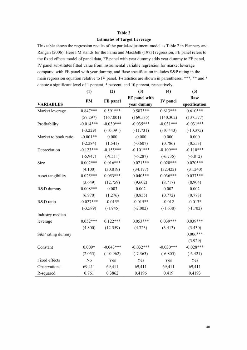
40

Table 2

Estimates of Target Leverage

This table shows the regression results of the partial-adjustment model as Table 2 in Flannery and

Rangan (2006). Here FM stands for the Fama and MacBeth (1973) regression, FE panel refers to

the fixed effects model of panel data, FE panel with year dummy adds year dummy to FE panel,

IV panel substitutes fitted value from instrumental variable regression for market leverage

compared with FE panel with year dummy, and Base specification includes S&P rating in the

main regression equation relative to IV panel. T-statistics are shown in parentheses. ***, ** and *

denote a significant level of 1 percent, 5 percent, and 10 percent, respectively.

(1) (2) (3) (4) (5)

VARIABLES FM FE panel

FE panel with

year dummy IV panel

Base

specification

Market leverage 0.847*** 0.591*** 0.587*** 0.613*** 0.610***

(57.297) (167.001) (169.535) (140.302) (137.577)

Profitability -0.014*** -0.030*** -0.035*** -0.031*** -0.031***

(-3.229) (-10.091) (-11.731) (-10.443) (-10.375)

Market to book ratio -0.001** 0.000 -0.000 0.000 0.000

(-2.284) (1.541) (-0.607) (0.786) (0.553)

Depreciation -0.123*** -0.155*** -0.101*** -0.109*** -0.110***

(-5.947) (-9.511) (-6.287) (-6.735) (-6.812)

Size 0.002*** 0.016*** 0.021*** 0.020*** 0.020***

(4.100) (30.819) (34.177) (32.422) (31.240)

Asset tangibility 0.025*** 0.053*** 0.040*** 0.036*** 0.037***

(3.649) (12.759) (9.602) (8.717) (8.904)

R&D dummy 0.008*** 0.003 0.002 0.002 0.002

(6.970) (1.276) (0.855) (0.772) (0.773)

R&D ratio -0.027*** -0.015* -0.015** -0.012 -0.013*

(-3.589) (-1.945) (-2.002) (-1.630) (-1.702)

Industry median

leverage 0.052*** 0.122*** 0.053*** 0.039*** 0.039***

(4.800) (12.559) (4.723) (3.413) (3.430)

S&P rating dummy 0.006***

(3.929)

Constant 0.009* -0.043*** -0.032*** -0.030*** -0.028***

(2.055) (-10.962) (-7.363) (-6.805) (-6.421)

Fixed effects No Yes Yes Yes Yes

Observations 69,411 69,411 69,411 69,411 69,411

R-squared 0.761 0.3862 0.4196 0.419 0.4193

41

Table 3

Distribution of Securities Issued by Year

This table shows the distribution of each type of security issued across years from 1988 to 2008.

Here we treat the multiple issues of the same type of security by one firm with one fiscal year as

one issue as an issuance may have several tranches. In addition, Column 5 shows the net

percentage of banks tightening standards for C&I loans to small firms from the Senior Loan

Officer Opinion Survey on Bank Lending Practices, and the last column shows the number of

Compustat firms in our sample each year.

Year Private equity SEO Loan

% of

Tightening

Standards

Bond Total

1988 7 35 319 54 2515

1989 14 54 348 59 2471

1990 16 47 384 52 2501

1991 7 148 382 13.10 94 2582

1992 17 121 465 -3.60 123 2737

1993 15 178 493 -5.95 143 2955

1994 7 123 696 -11.43 74 3172

1995 12 162 675 -3.95 127 3307

1996 10 236 811 -2.20 140 3534

1997 14 190 960 -3.55 194 3773

1998 5 133 785 2.43 232 3769

1999 17 144 720 3.95 180 3649

2000 32 164 745 20.43 105 3675

2001 89 129 831 38.45 214 3738

2002 102 127 844 20.00 201 3708

2003 114 159 800 7.05 245 3656

2004 119 184 977 -13.03 241 3576

2005 81 146 986 -13.35 193 3548

2006 97 138 906 -4.43 181 3508

2007 113 147 814 6.13 186 3481

2008 96 96 558 55.50 142 3556

Total 984 2861 14499 3180 69411

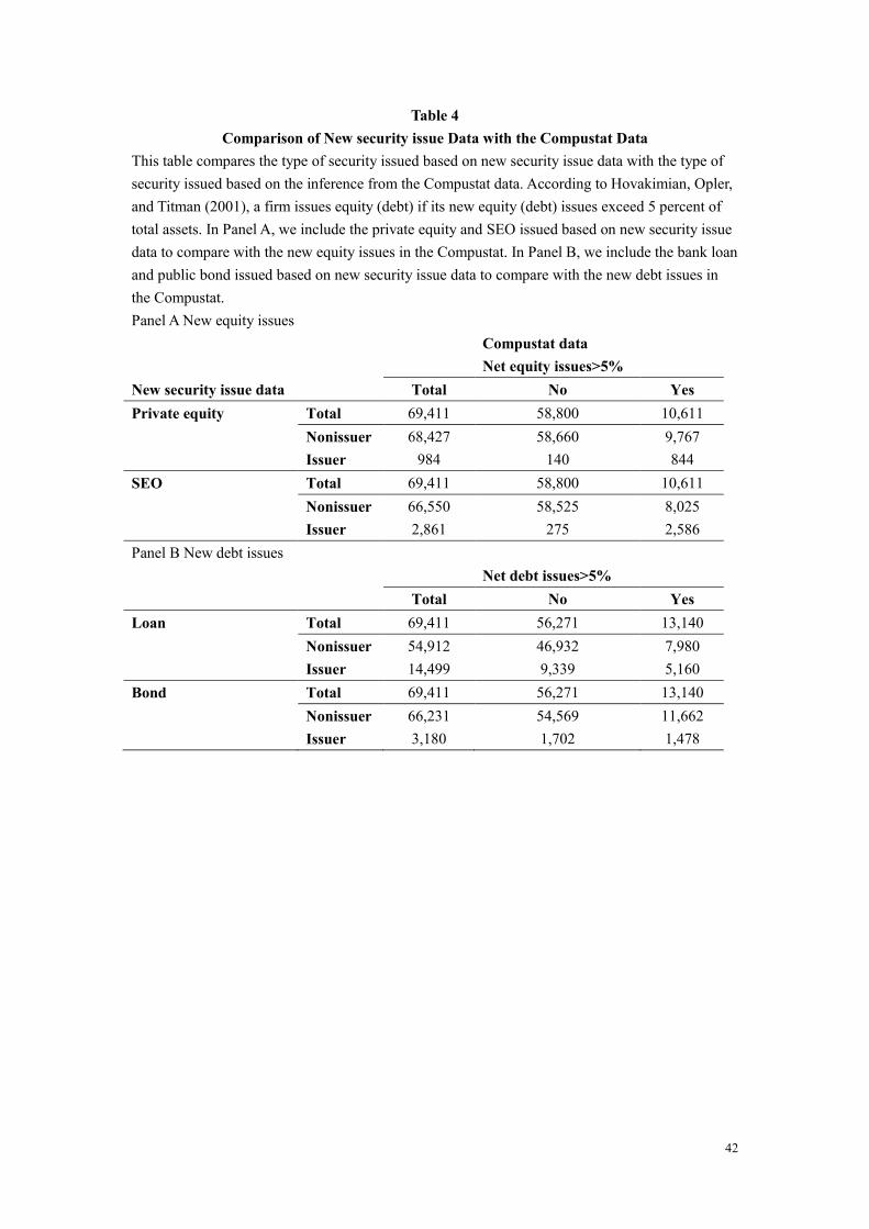
42

Table 4

Comparison of New security issue Data with the Compustat Data

This table compares the type of security issued based on new security issue data with the type of

security issued based on the inference from the Compustat data. According to Hovakimian, Opler,

and Titman (2001), a firm issues equity (debt) if its new equity (debt) issues exceed 5 percent of

total assets. In Panel A, we include the private equity and SEO issued based on new security issue

data to compare with the new equity issues in the Compustat. In Panel B, we include the bank loan

and public bond issued based on new security issue data to compare with the new debt issues in

the Compustat.

Panel A New equity issues

Compustat data

Net equity issues>5%

New security issue data Total No Yes

Private equity Total 69,411 58,800 10,611

Nonissuer 68,427 58,660 9,767

Issuer 984 140 844

SEO Total 69,411 58,800 10,611

Nonissuer 66,550 58,525 8,025

Issuer 2,861 275 2,586

Panel B New debt issues

Net debt issues>5%

Total No Yes

Loan Total 69,411 56,271 13,140

Nonissuer 54,912 46,932 7,980

Issuer 14,499 9,339 5,160

Bond Total 69,411 56,271 13,140

Nonissuer 66,231 54,569 11,662

Issuer 3,180 1,702 1,478

43

Table 5

Comparison of the Four Financial Constraints Measures

This table compares the four financial constraints measures. Panel A shows the correlation matrix

between the constrained and unconstrained firms based on any two of the criteria. Panel B shows

the key firm characteristics for the constrained and unconstrained firms defined by each measure.

Panel A Correlation between financial constraints criteria

Financial

constraints criteria Payout ratio KZ index WW index SA index

Payout ratio

C U C U C U C U

Constrained firms C 33,756

Unconstrained firms U 20,807

KZ index

Constrained firms C 12,538 2,750 20,493

Unconstrained firms U 9,572 8,286 20,512

WW index

Constrained firms C 16,376 2,050 6,911 6,228 20,265

Unconstrained firms U 2,563 11,062 5,044 5,472 20,282

SA index

Constrained firms C 16,138 2,517 5,381 8,255 14,970 404 20,730

Unconstrained firms U 3,957 10,710 5,592 5,066 522 13,883 20,755

Panel B Key firm characteristics based on each financial constraints criterion

Mean

Payout ratio KZ index WW index SA index

Firm characteristics C U C U C U C U

Analyst coverage 1.73 6.10 2.66 3.31 0.72 7.63 0.48 7.70

Tangible assets 0.25 0.32 0.43 0.13 0.22 0.37 0.22 0.34

S&P rating 0.12 0.36 0.31 0.14 0.01 0.59 0.00 0.54

Private equity 2.47% 0.41% 1.88% 1.40% 2.96% 0.54% 3.37% 0.34%

SEO 5.45% 2.24% 4.78% 4.41% 3.94% 3.05% 5.20% 2.58%

Loan 16.36% 24.29% 27.53% 13.08% 10.20% 30.91% 9.45% 29.85%

Bond 2.05% 7.49% 6.44% 2.67% 0.19% 12.03% 0.13% 10.97%

Size 4.68 6.62 5.61 5.26 3.57 7.87 3.48 7.41

Market to book ratio 2.50 1.92 1.88 2.82 2.42 1.90 2.90 1.71

R&D ratio 0.08 0.02 0.04 0.07 0.09 0.02 0.10 0.02

Depreciation 0.05 0.05 0.06 0.03 0.05 0.05 0.05 0.05

Median

C U C U C U C U

Analyst coverage 0 2 0 0 0 4 0 4

Tangible assets 0.17 0.27 0.40 0.09 0.15 0.32 0.14 0.29

S&P rating 0 0 0 0 0 1 0 1

Size 4.57 6.57 5.59 5.01 3.68 7.80 3.58 7.32

Market to book ratio 1.69 1.53 1.29 2.10 1.64 1.47 2.01 1.69

R&D ratio 0.02 0 0 0.04 0.04 0 0.04 0.02

Depreciation 0.04 0.04 0.05 0.03 0.04 0.04 0.04 0.04

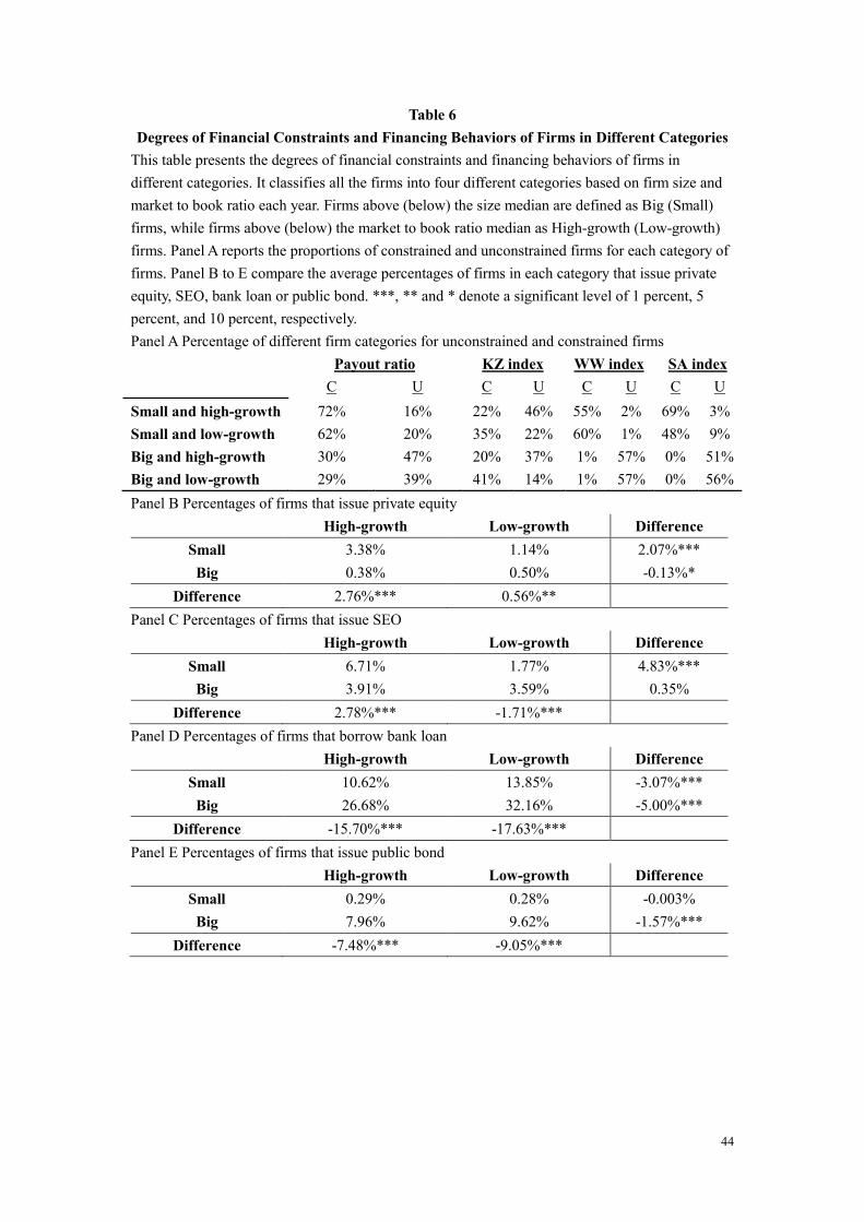
44

Table 6

Degrees of Financial Constraints and Financing Behaviors of Firms in Different Categories

This table presents the degrees of financial constraints and financing behaviors of firms in

different categories. It classifies all the firms into four different categories based on firm size and

market to book ratio each year. Firms above (below) the size median are defined as Big (Small)

firms, while firms above (below) the market to book ratio median as High-growth (Low-growth)

firms. Panel A reports the proportions of constrained and unconstrained firms for each category of

firms. Panel B to E compare the average percentages of firms in each category that issue private

equity, SEO, bank loan or public bond. ***, ** and * denote a significant level of 1 percent, 5

percent, and 10 percent, respectively.

Panel A Percentage of different firm categories for unconstrained and constrained firms

Payout ratio KZ index WW index SA index

C U C U C U C U

Small and high-growth 72% 16% 22% 46% 55% 2% 69% 3%

Small and low-growth 62% 20% 35% 22% 60% 1% 48% 9%

Big and high-growth 30% 47% 20% 37% 1% 57% 0% 51%

Big and low-growth 29% 39% 41% 14% 1% 57% 0% 56%

Panel B Percentages of firms that issue private equity

High-growth Low-growth Difference

Small 3.38% 1.14% 2.07%***

Big 0.38% 0.50% -0.13%*

Difference 2.76%*** 0.56%**

Panel C Percentages of firms that issue SEO

High-growth Low-growth Difference

Small 6.71% 1.77% 4.83%***

Big 3.91% 3.59% 0.35%

Difference 2.78%*** -1.71%***

Panel D Percentages of firms that borrow bank loan

High-growth Low-growth Difference

Small 10.62% 13.85% -3.07%***

Big 26.68% 32.16% -5.00%***

Difference -15.70%*** -17.63%***

Panel E Percentages of firms that issue public bond

High-growth Low-growth Difference

Small 0.29% 0.28% -0.003%

Big 7.96% 9.62% -1.57%***

Difference -7.48%*** -9.05%***

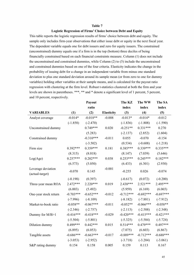
45

Table 7

Logistic Regression of Firms’ Choice between Debt and Equity

This table reports the logistic regression results of firms’ choice between debt and equity. The

sample only includes firm-year observations that either issue debt or equity in the next fiscal year.

The dependent variable equals one for debt issuers and zero for equity issuers. The constrained

(unconstrained) dummy equals one if a firm is in the top (bottom) three deciles of being

financially constrained based on each financial constraints measure. Column (1) does not include

the unconstrained and constrained dummies, while Column (2) to (5) include the unconstrained

and constrained dummies based on one of the four criteria. Elasticity indicates the change in the

probability of issuing debt for a change in an independent variable from minus one standard

deviation to plus one standard deviation around its sample mean (or from zero to one for dummy

variables) holding other variables at their sample means, and is calculated for the payout ratio

regression with clustering at the firm level. Robust t-statistics clustered at both the firm and year

levels are shown in parentheses. ***, ** and * denote a significant level of 1 percent, 5 percent,

and 10 percent, respectively.

Payout

ratio

The KZ

index

The WW

index

The SA

index

VARIABLES (1) (2) Elasticity (3) (4) (5)

Analyst coverage -0.014* -0.018** -0.008 -0.013* -0.014* -0.012

(-1.858) (-2.470) (-1.836) (-1.808) (-1.590)

Unconstrained dummy

0.749*** 0.020 -0.251** 0.331*** 0.270

(5.283) (-2.137) (2.852) (1.604)

Constrained dummy

-0.310*** -0.011 0.055 -0.070 -0.154

(-3.502) (0.534) (-0.608) (-1.218)

Firm size 0.392*** 0.359*** 0.181 0.385*** 0.339*** 0.335***

(8.315) (8.018) (8.147) (7.039) (5.646)

Log(Age) 0.257*** 0.202*** 0.038 0.253*** 0.245*** 0.182***

(6.573) (5.050) (6.433) (6.301) (2.930)

Leverage deviation

(actual-target) -0.070 0.145

-0.001 -0.255 0.026 -0.074

(-0.198) (0.397) (-0.617) (0.072) (-0.200)

Three-year mean ROA 2.472*** 2.220*** 0.019 2.438*** 2.521*** 2.495***

(6.003) (5.492) (5.959) (6.169) (6.065)

One-year stock return -0.703*** -0.652*** -0.012 -0.712*** -0.692*** -0.697***

(-7.996) (-8.109) (-8.182) (-7.881) (-7.912)

Market-to-book ratio -0.058** -0.067*** -0.011 -0.052** -0.066*** -0.058**

(-2.346) (-2.757) (-2.113) (-2.588) (-2.348)

Dummy for M/B>1 -0.416*** -0.418*** -0.029 -0.420*** -0.415*** -0.421***

(-5.504) (-5.801) (-5.325) (-5.584) (-5.724)

Dilution dummy 0.499*** 0.442*** 0.015 0.514*** 0.479*** 0.497***

(6.895) (6.053) (7.075) (6.603) (6.867)

Tangible assets -0.686*** -0.663*** -0.017 -0.889*** -0.712*** -0.688***

(-3.053) (-2.952) (-3.718) (-3.204) (-3.061)

S&P rating dummy 0.154 0.158 0.005 0.159 0.113 0.167

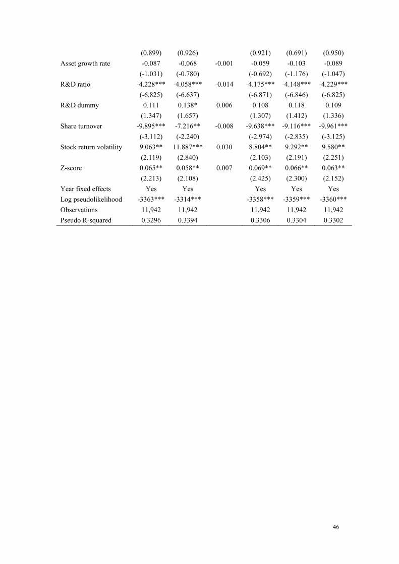
46

(0.899) (0.926) (0.921) (0.691) (0.950)

Asset growth rate -0.087 -0.068 -0.001 -0.059 -0.103 -0.089

(-1.031) (-0.780) (-0.692) (-1.176) (-1.047)

R&D ratio -4.228*** -4.058*** -0.014 -4.175*** -4.148*** -4.229***

(-6.825) (-6.637) (-6.871) (-6.846) (-6.825)

R&D dummy 0.111 0.138* 0.006 0.108 0.118 0.109

(1.347) (1.657) (1.307) (1.412) (1.336)

Share turnover -9.895*** -7.216** -0.008 -9.638*** -9.116*** -9.961***

(-3.112) (-2.240) (-2.974) (-2.835) (-3.125)

Stock return volatility 9.063** 11.887*** 0.030 8.804** 9.292** 9.580**

(2.119) (2.840) (2.103) (2.191) (2.251)

Z-score 0.065** 0.058** 0.007 0.069** 0.066** 0.063**

(2.213) (2.108) (2.425) (2.300) (2.152)

Year fixed effects Yes Yes Yes Yes Yes

Log pseudolikelihood -3363*** -3314*** -3358*** -3359*** -3360***

Observations 11,942 11,942 11,942 11,942 11,942

Pseudo R-squared 0.3296 0.3394 0.3306 0.3304 0.3302

47

Table 8

The Multinomial Logistic Regression with Payout Ratio

This table reports the multinomial logistic regression results of firms’ choice among private equity,

SEO, bank loan and public bond using firms issuing SEO as base outcome. Robust t-statistics

clustered at the firm level are shown in parentheses. ***, ** and * denote a significant level of 1

percent, 5 percent, and 10 percent, respectively.

(1) (2)

VARIABLES

Private

equity Loan Bond

Private

equity Loan Bond

Analyst coverage 0.046** -0.014* 0.012 0.048** -0.016** 0.010

(2.313) (-1.933) (1.446) (2.392) (-2.235) (1.143)

Payout ratio decile 0.030 0.111*** 0.112***

(1.081) (8.382) (5.748)

Firm size -0.536*** 0.267*** 0.689*** -0.552*** 0.231*** 0.652***

(-6.165) (7.033) (11.677) (-6.322) (6.085) (11.026)

Log(Age) 0.262*** 0.307*** 0.301*** 0.241*** 0.245*** 0.240***

(3.372) (7.604) (4.493) (3.060) (5.974) (3.534)

Leverage deviation

(actual-target) -1.022* -0.425 0.423 -0.930 -0.253 0.600

(-1.670) (-1.371) (0.871) (-1.530) (-0.817) (1.236)

Three-year mean ROA -1.079*** 2.342*** 1.604* -1.105*** 2.061*** 1.327

(-2.686) (6.363) (1.843) (-2.725) (5.764) (1.546)

One-year stock return -0.355*** -0.799*** -0.707*** -0.347*** -0.761*** -0.666***

(-3.138) (-11.266) (-6.006) (-3.068) (-10.761) (-5.668)

Market-to-book ratio -0.103** -0.077*** 0.056 -0.105*** -0.084*** 0.048

(-2.530) (-3.026) (0.934) (-2.580) (-3.286) (0.810)

Dummy for M/B>1 -0.230 -0.515*** -0.203 -0.210 -0.507*** -0.192

(-0.895) (-3.710) (-1.044) (-0.821) (-3.621) (-0.990)

Dilution dummy -0.300 0.458*** 0.620*** -0.310 0.392*** 0.556***

(-1.387) (5.155) (5.163) (-1.436) (4.364) (4.620)

Tangible assets 0.507 -0.715*** -0.134 0.488 -0.739*** -0.159

(1.312) (-3.612) (-0.452) (1.263) (-3.735) (-0.534)

S&P rating dummy 0.256 0.042 1.698*** 0.251 0.035 1.691***

(0.943) (0.371) (9.792) (0.930) (0.307) (9.759)

Asset growth rate 0.124 -0.079 0.196** 0.137 -0.061 0.214**

(1.459) (-1.149) (2.047) (1.581) (-0.885) (2.253)

R&D ratio -1.230** -4.769*** -3.530** -1.195** -4.668*** -3.422**

(-2.168) (-8.591) (-2.302) (-2.095) (-8.562) (-2.258)

R&D dummy -0.039 0.105 0.131 -0.014 0.120 0.147

(-0.207) (1.130) (0.927) (-0.077) (1.274) (1.032)

Share turnover -9.897* -10.537*** -32.888*** -8.922* -8.097*** -30.357***

(-1.894) (-3.792) (-5.957) (-1.690) (-2.910) (-5.506)

Stock return volatility 19.519*** 12.758*** -0.408 21.129*** 16.058*** 3.324

(2.989) (3.196) (-0.059) (3.186) (3.941) (0.477)

48

Z-score -0.096*** 0.010 -0.062 -0.098*** 0.000 -0.072

(-3.141) (0.345) (-1.095) (-3.184) (0.009) (-1.285)

Constant -0.034 0.648 -5.656*** -0.123 0.489 -5.837***

(-0.041) (1.532) (-8.615) (-0.147) (1.155) (-8.931)

Year fixed effects Yes Yes Yes Yes Yes Yes

Log likelihood -6696*** -6647***

Observations 11,942 11,940

Pseudo R-squared 0.3153 0.3199

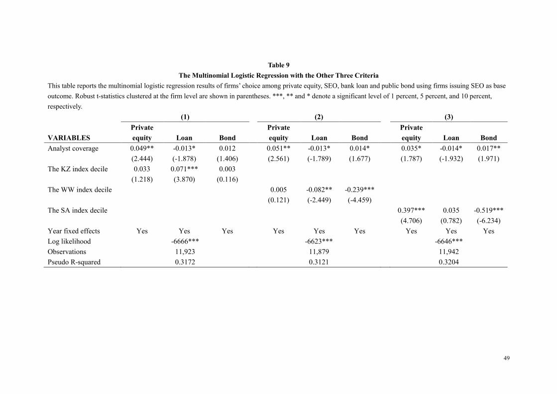
49

Table 9

The Multinomial Logistic Regression with the Other Three Criteria

This table reports the multinomial logistic regression results of firms’ choice among private equity, SEO, bank loan and public bond using firms issuing SEO as base

outcome. Robust t-statistics clustered at the firm level are shown in parentheses. ***, ** and * denote a significant level of 1 percent, 5 percent, and 10 percent,

respectively.

(1) (2) (3)

VARIABLES

Private

equity Loan Bond

Private

equity Loan Bond

Private

equity Loan Bond

Analyst coverage 0.049** -0.013* 0.012 0.051** -0.013* 0.014* 0.035* -0.014* 0.017**

(2.444) (-1.878) (1.406) (2.561) (-1.789) (1.677) (1.787) (-1.932) (1.971)

The KZ index decile 0.033 0.071*** 0.003

(1.218) (3.870) (0.116)

The WW index decile 0.005 -0.082** -0.239***

(0.121) (-2.449) (-4.459)

The SA index decile 0.397*** 0.035 -0.519***

(4.706) (0.782) (-6.234)

Year fixed effects Yes Yes Yes Yes Yes Yes Yes Yes Yes

Log likelihood -6666*** -6623*** -6646***

Observations 11,923 11,879 11,942

Pseudo R-squared 0.3172 0.3121 0.3204

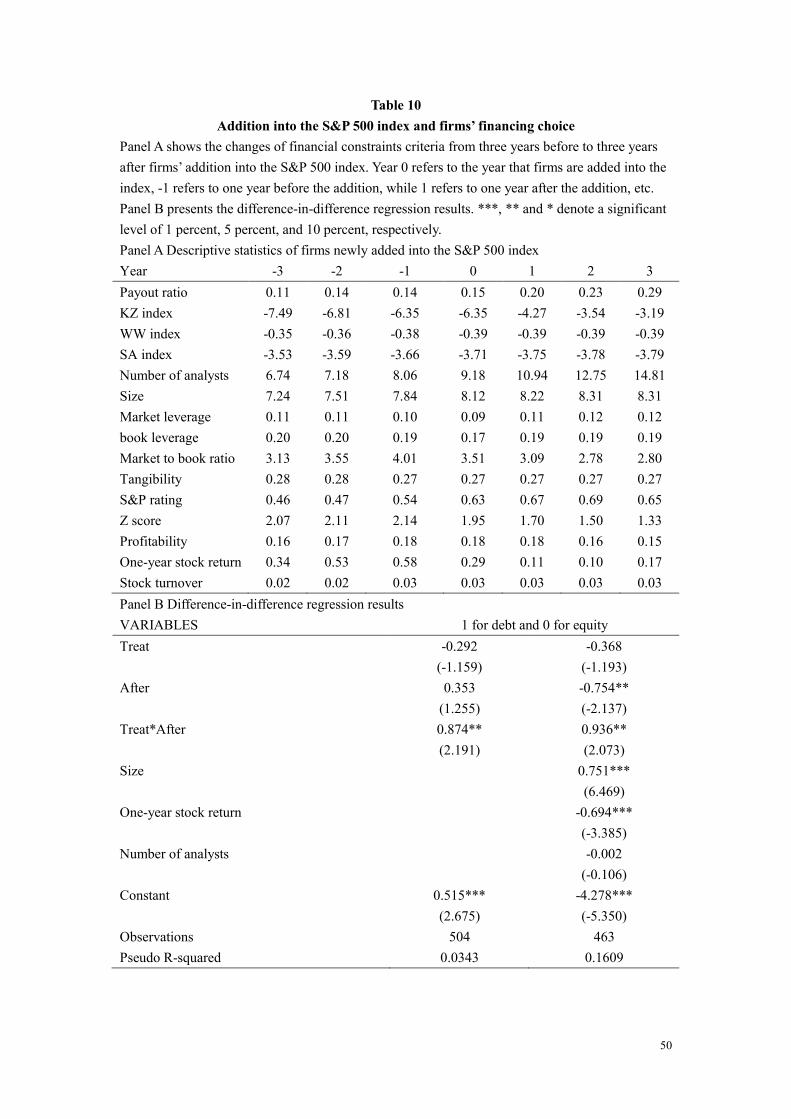
50

Table 10

Addition into the S&P 500 index and firms’ financing choice

Panel A shows the changes of financial constraints criteria from three years before to three years

after firms’ addition into the S&P 500 index. Year 0 refers to the year that firms are added into the

index, -1 refers to one year before the addition, while 1 refers to one year after the addition, etc.

Panel B presents the difference-in-difference regression results. ***, ** and * denote a significant

level of 1 percent, 5 percent, and 10 percent, respectively.

Panel A Descriptive statistics of firms newly added into the S&P 500 index

Year -3 -2 -1 0 1 2 3

Payout ratio 0.11 0.14 0.14 0.15 0.20 0.23 0.29

KZ index -7.49 -6.81 -6.35 -6.35 -4.27 -3.54 -3.19

WW index -0.35 -0.36 -0.38 -0.39 -0.39 -0.39 -0.39

SA index -3.53 -3.59 -3.66 -3.71 -3.75 -3.78 -3.79

Number of analysts 6.74 7.18 8.06 9.18 10.94 12.75 14.81

Size 7.24 7.51 7.84 8.12 8.22 8.31 8.31

Market leverage 0.11 0.11 0.10 0.09 0.11 0.12 0.12

book leverage 0.20 0.20 0.19 0.17 0.19 0.19 0.19

Market to book ratio 3.13 3.55 4.01 3.51 3.09 2.78 2.80

Tangibility 0.28 0.28 0.27 0.27 0.27 0.27 0.27

S&P rating 0.46 0.47 0.54 0.63 0.67 0.69 0.65

Z score 2.07 2.11 2.14 1.95 1.70 1.50 1.33

Profitability 0.16 0.17 0.18 0.18 0.18 0.16 0.15

One-year stock return 0.34 0.53 0.58 0.29 0.11 0.10 0.17

Stock turnover 0.02 0.02 0.03 0.03 0.03 0.03 0.03

Panel B Difference-in-difference regression results

VARIABLES 1 for debt and 0 for equity

Treat -0.292 -0.368

(-1.159) (-1.193)

After 0.353 -0.754**

(1.255) (-2.137)

Treat*After 0.874** 0.936**

(2.191) (2.073)

Size 0.751***

(6.469)

One-year stock return -0.694***

(-3.385)

Number of analysts -0.002

(-0.106)

Constant 0.515*** -4.278***

(2.675) (-5.350)

Observations 504 463

Pseudo R-squared 0.0343 0.1609

51

Table 11

Shyam-Sunder and Myers (1999) and Lemmon and Zender (2010) Regression Results

This table reports the Shyam-Sunder and Myers (1999) regression and Lemmon and Zender (2010)

modified regression results for different types of firms based on the SA index. We first classify the

sample into deciles based on the SA index, and then define the top (bottom) three deciles as

financially constrained (unconstrained) firms, while define firms in-between as intermediate firms.

Robust t-statistics clustered at both the firm and year levels are shown in parentheses. ***, ** and

* denote a significant level of 1 percent, 5 percent, and 10 percent, respectively.

VARIABLES Constrained firms Intermediate firms Unconstrained firms

Financing deficit 0.016*** 0.067*** 0.135*** 0.424*** 0.450*** 0.720***

(3.522) (5.858) (5.131) (15.131) (16.568) (26.137)

Squared financing deficit -0.012*** -0.076*** -0.139***

(-6.051) (-15.169) (-11.170)

Constant -0.000 -0.007*** 0.019*** 0.000 0.012*** 0.010***

(-0.120) (-4.466) (4.522) (0.186) (4.969) (4.650)

Observations 18,991 18,991 25,467 25,467 19,107 19,107

R-squared 0.015 0.032 0.191 0.377 0.531 0.664

52

Figure 1 (a) Unconstrained firms

Figure 1 (b) Intermediate firms

Figure 1 (c) Constrained firms

Figure 1 Financing deficit, net debt issues and net equity issues. Figure 1 graphs the

relationship among financing deficit, net debt issues and net equity issues for the unconstrained,

intermediate and constrained firms, respectively. We classify the firms into deciles based on the

SA index in each year, and define firms in the top (bottom) three deciles as financially constrained

(unconstrained) firms, while firms in-between as the intermediate firms. Here the SA index is

calculated as - 0.737 × Size + 0.043 × Size2- 0.040 × Age as in Hadlock and Pierce (2010),

where Size and Age have a upper bond of log($4.5 billion) and 37 years, respectively. The higher

the SA index is, the more financial constraints a firm faces.

-0.02

-0.01

0

0.01

0.02

0.03

0.04

0.05

0.06

0.07 Net debt issues Net equity issues

Financing deficit

-0.1

0

0.1

0.2

0.3

0.4 Net debt issues Net equity issues

Financing deficit

-0.2

0

0.2

0.4

0.6

0.8

1 Net debt issues Net equity issues

Financing deficit