Embed Size (px)
Citation preview
Testing the EH Antenna ~ Page 1antenneX ~ February 2003
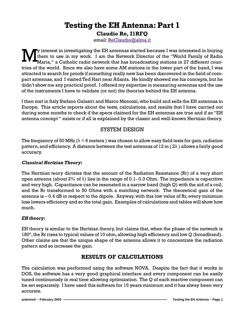
Testing the EH Antenna: Part 1Claudio Re, I1RFQ
email: [email protected]
My interest in investigating the EH antennas started because I was interested in buyingthem to use in my work. I am the Network Director of the “World Family of RadioMaria,“ a Catholic radio network that has broadcasting stations in 27 different coun-
tries of the world. Since we also have some AM stations in the lower part of the band, I wasattracted to search for proofs if something really new has been discovered in the field of com-pact antennas, and I visited Ted Hart near Atlanta. He kindly showed me his concepts, but hedidn’t show me any practical proof. I offered my expertise in measuring antennas and the useof the instruments I have to validate (or not) the theories behind the EH antenna.
I then met in Italy Stefano Galastri and Marco Menozzi, who build and sells the EH antennas inEurope. This article reports about the tests, calculations, and results that I have carried outduring some months to check if the specs claimed for the EH antennas are true and if an “EHantenna concept “ exists or if all is explained by the classic and well-known Hertzian theory.
SYSTEM DESIGN
The frequency of 50 MHz (λ = 6 meters ) was chosen to allow easy field tests for gain, radiationpattern, and efficiency. A distance between the test antennas of 12 m ( 2λ ) allows a fairly goodaccuracy.
Classical Hertzian Theory:
The Hertzian teory dictates that the amount of the Radiation Resistance (Rr) of a very shortopen antenna (about 2% of λ) lies in the range of 0.1- 0.3 Ohm. The impedance is capacitiveand very high. Capacitance can be resonated in a narrow band (high Q) with the aid of a coil,and the Rr transformed to 50 Ohms with a matching network. The theoretical gain of theantenna is – 0.4 dB in respect to the dipole. Anyway, with this low value of Rr, every minimumloss lowers efficiency and so the total gain. Examples of calculations and tables will show howmuch.
EH theory:
EH theory is similar to the Hertzian theory, but claims that, when the phase of the network is180°, the Rr rises to typical values of 10 ohm, allowing high efficiency and low Q (broadband).Other claims are that the unique shape of the antenna allows it to concentrate the radiationpattern and so increase the gain.
RESULTS OF CALCULATIONS
The calculation was performed using the software NOVA. Despite the fact that it works inDOS, the software has a very good graphical interface and every component can be easilytuned continuously in real time allowing optimization. The Q of each reactive component canbe set separately. I have used this software for 15 years minimum and it has alway been veryaccurate.
Testing the EH Antenna ~ Page 2antenneX ~ February 2003
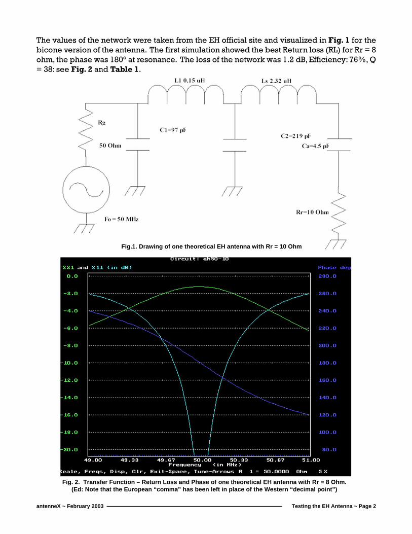
The values of the network were taken from the EH official site and visualized in Fig. 1 for thebicone version of the antenna. The first simulation showed the best Return loss (RL) for Rr = 8ohm, the phase was 180° at resonance. The loss of the network was 1.2 dB, Efficiency: 76%, Q= 38: see Fig. 2 and Table 1.
Fig.1. Drawing of one theoretical EH antenna with Rr = 10 Ohm
Fig. 2. Transfer Function – Return Loss and Phase of one theoretical EH antenna with Rr = 8 Ohm.(Ed: Note that the European “comma” has been left in place of the Western “decimal point”)
Testing the EH Antenna ~ Page 3antenneX ~ February 2003
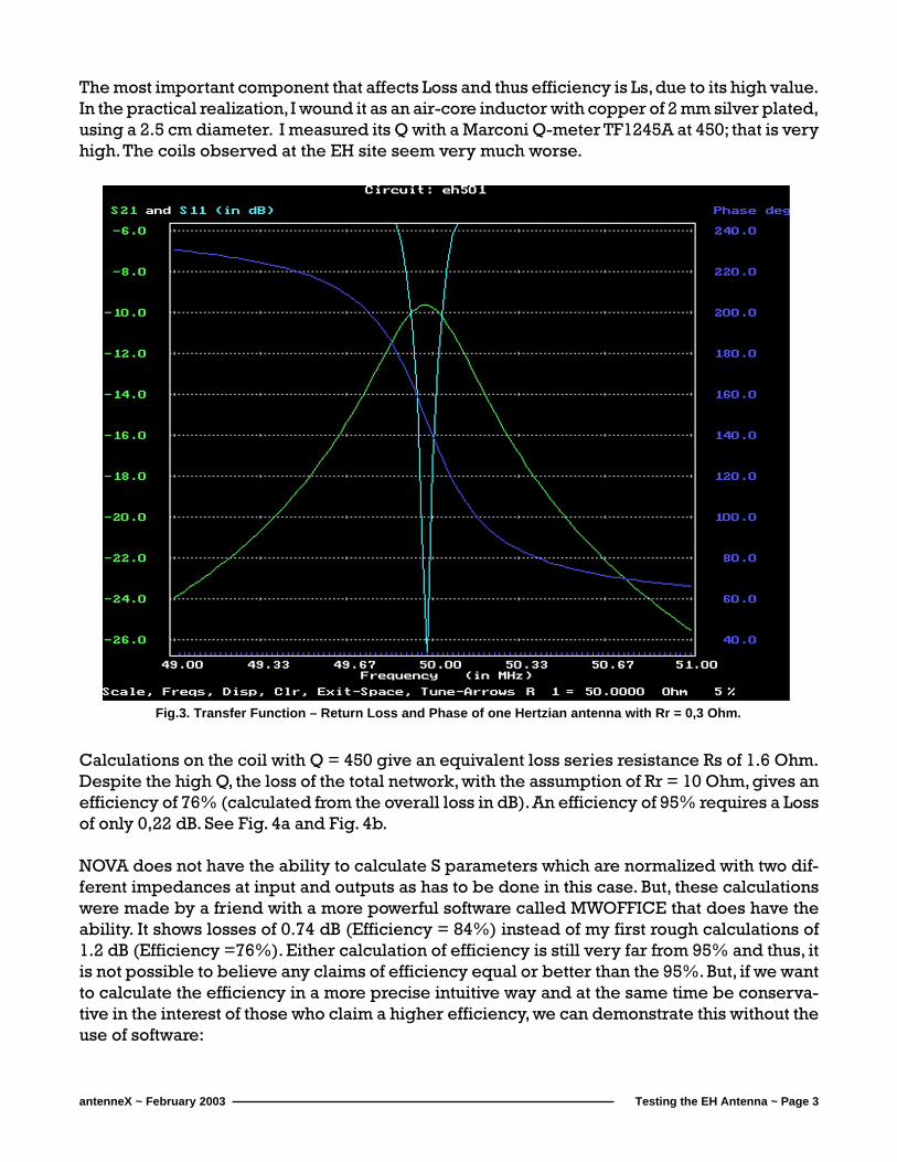
The most important component that affects Loss and thus efficiency is Ls, due to its high value.In the practical realization, I wound it as an air-core inductor with copper of 2 mm silver plated,using a 2.5 cm diameter. I measured its Q with a Marconi Q-meter TF1245A at 450; that is veryhigh. The coils observed at the EH site seem very much worse.
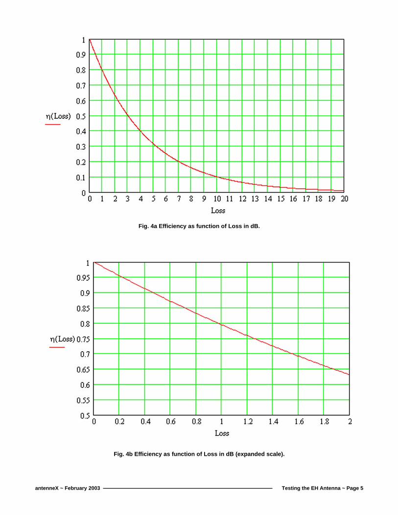
Calculations on the coil with Q = 450 give an equivalent loss series resistance Rs of 1.6 Ohm.Despite the high Q, the loss of the total network, with the assumption of Rr = 10 Ohm, gives anefficiency of 76% (calculated from the overall loss in dB). An efficiency of 95% requires a Lossof only 0,22 dB. See Fig. 4a and Fig. 4b.
NOVA does not have the ability to calculate S parameters which are normalized with two dif-ferent impedances at input and outputs as has to be done in this case. But, these calculationswere made by a friend with a more powerful software called MWOFFICE that does have theability. It shows losses of 0.74 dB (Efficiency = 84%) instead of my first rough calculations of1.2 dB (Efficiency =76%). Either calculation of efficiency is still very far from 95% and thus, itis not possible to believe any claims of efficiency equal or better than the 95%. But, if we wantto calculate the efficiency in a more precise intuitive way and at the same time be conserva-tive in the interest of those who claim a higher efficiency, we can demonstrate this without theuse of software:
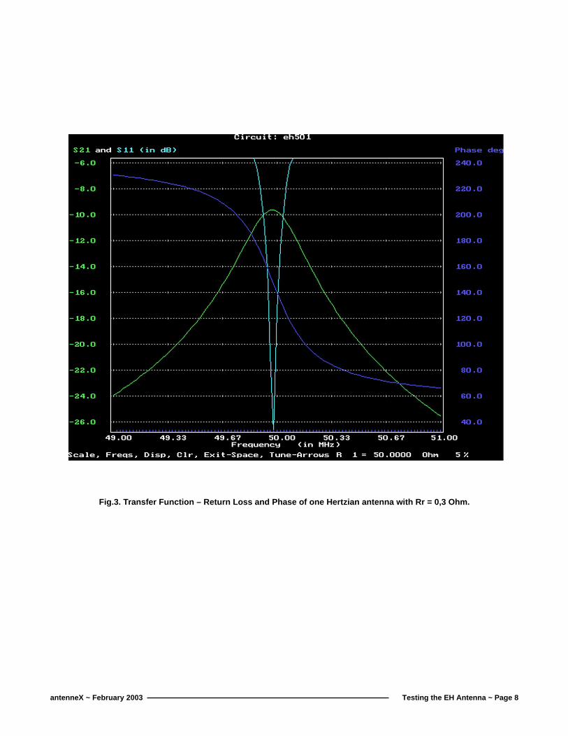
Fig.3. Transfer Function – Return Loss and Phase of one Hertzian antenna with Rr = 0,3 Ohm.

Testing the EH Antenna ~ Page 4antenneX ~ February 2003
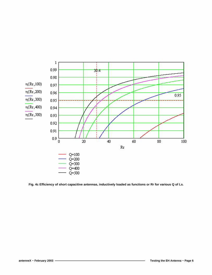
If we want to calculate what Rr is needed to have an efficiency of 95 %, assuming the mostfavourable condition that losses are only due to the Rs of Ls, we calculate this way:
ηηηηη = Rr/(Rs+Rr) = 0.95
Solving for Rr:
Rr = 19Rs = 30.4 Ohm.
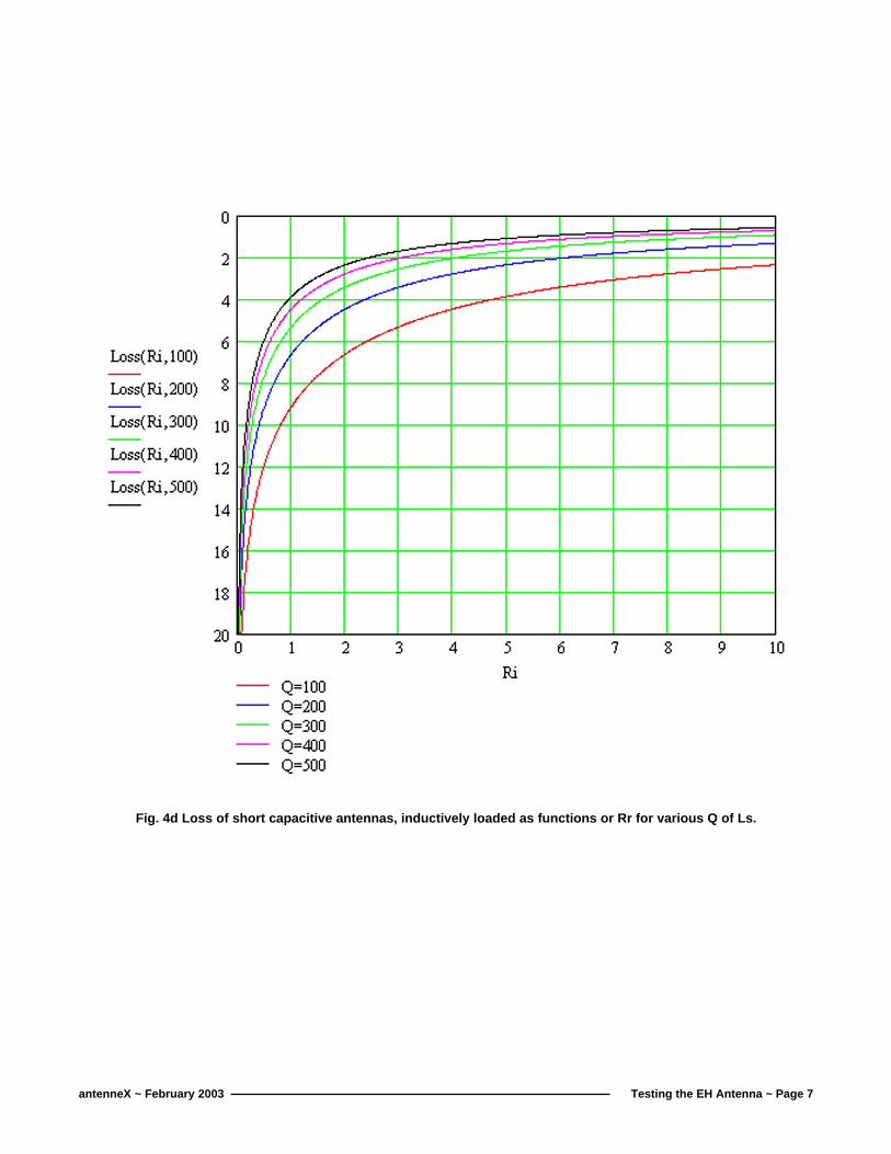
It is easy to understand that this value is outside of discussion for the small antenna. Thegraphics of the calculations for Efficiency and Loss respect to Rr, made for various Q, areplotted in Fig. 4c and Fig. 4d, and once again clearly demonstrate the thesis, showing thepoints at ηηηηη = 95 % for various Q (Rr = 30.4 Ohm for Q = 450). Just for example, you can see thatwith a Q = 100 you never reach 95 % of efficiency even if Rr = 100 Ohm! Further physical proofwill also be shown in other parts of the article.
Fig.4. Transfer Function – Return Loss and Phase of one Hertzian antennawith Rr = 0,3 Ohm –Phase 180° at resonance.
Table 1
Testing the EH Antenna ~ Page 5antenneX ~ February 2003
Fig. 4a Efficiency as function of Loss in dB.
Fig. 4b Efficiency as function of Loss in dB (expanded scale).
Testing the EH Antenna ~ Page 6antenneX ~ February 2003
Fig. 4c Efficiency of short capacitive antennas, inductively loaded as functions or Rr for various Q of Ls.
Testing the EH Antenna ~ Page 7antenneX ~ February 2003
Fig. 4d Loss of short capacitive antennas, inductively loaded as functions or Rr for various Q of Ls.
Testing the EH Antenna ~ Page 8antenneX ~ February 2003
Fig.3. Transfer Function – Return Loss and Phase of one Hertzian antenna with Rr = 0,3 Ohm.
Testing the EH Antenna ~ Page 9antenneX ~ February 2003
The second simulation was made with Rr = 0.3 Ohm. I tried to return to the same RL by chang-ing the minimum of the values. This was achieved only by changing L1 from 0.15 to 0.22 µH.See Fig. 3 and Table 1, with values of Loss, Q, Efficiency and Phase.
The third simulation was to change the minimum of components to have 180° at resonance.This was achieved with L1 = 0.25 µH and C1 = 52 pF, with no change on Q, RL and Loss. SeeFig. 4 and Table 1.
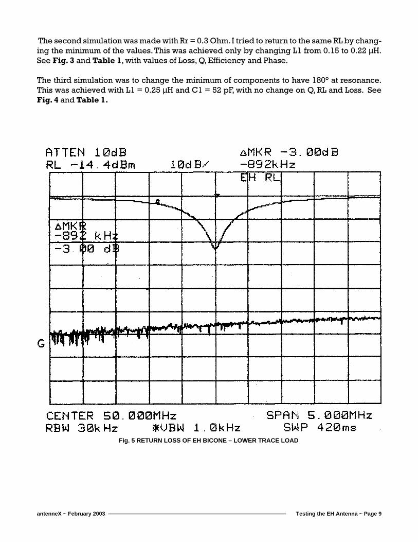
Fig. 5 RETURN LOSS OF EH BICONE – LOWER TRACE LOAD
Testing the EH Antenna ~ Page 10antenneX ~ February 2003
PRELIMINARY CONCLUSIONS BASED ON NETWORK CALCULATIONS
1) The calculations of efficiency of the network proposed at the EH site, even with veryhigh Q of the main coil (Ls), exclude the possibility of an efficiency equal or better than95 %.
2) If you can only measure the RL (or WSVR), at resonance, you can have the same valuewith Rr = 8 or 0,3 Ohm, only by changing the value of L1 (0.15 µH), the little coil of thematching network, by less than 50% (0.22µH).
ANTENNA MEASUREMENTS
I built a bicone EH antenna with the values of Fig. 1 and Table 1. All the values were checkedwith the Marconi TF1245A Q-meter. The values of RL and Q were very dependent on theposition of the coaxial cable relative to other objects. This clearly indicates that RF currentsare flowing on the shield of the coaxial cable that radiates and is hence part of the antenna.
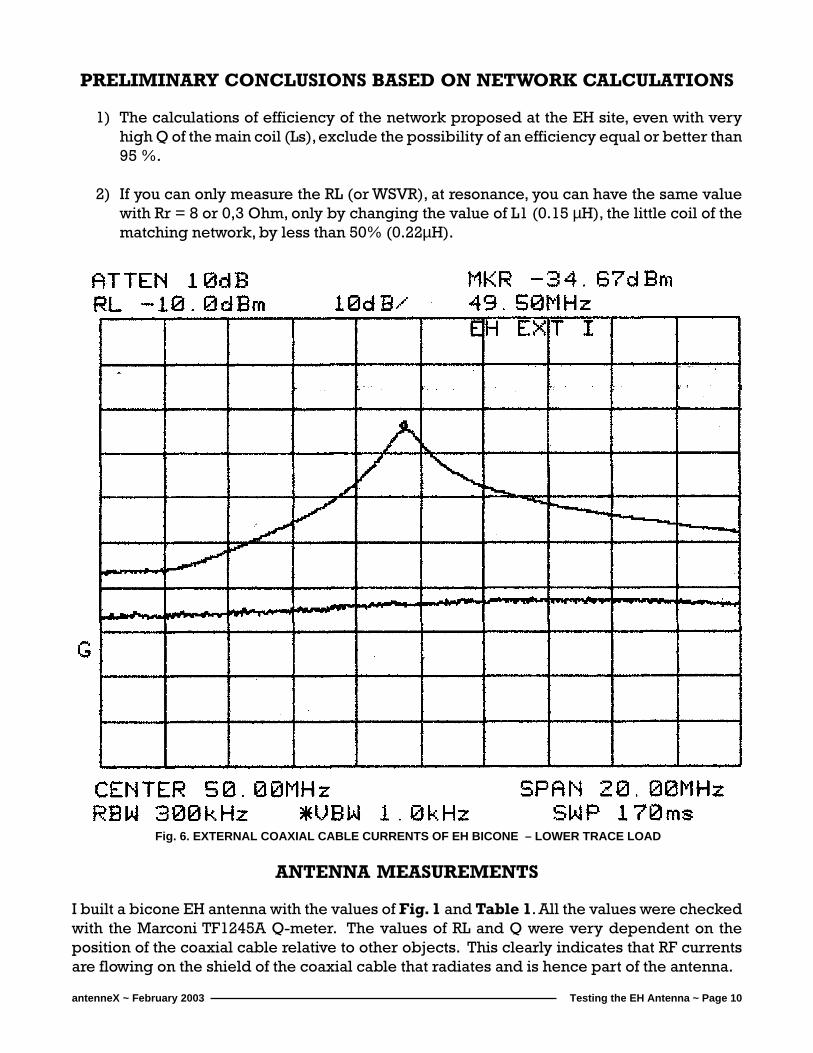
Fig. 6. EXTERNAL COAXIAL CABLE CURRENTS OF EH BICONE – LOWER TRACE LOAD
Testing the EH Antenna ~ Page 11antenneX ~ February 2003
To measure the external current, I built a tool consisting of a RF current transformer: a toroidalcore with an E shielded link connected to a BNC connector. The coaxial cable passes throughthe toroid. Values of RL and I (external current) of the cable at the base of the antenna areplotted in Fig. 5 and Fig. 6. Lower traces are the values connecting a load instead of theantenna.
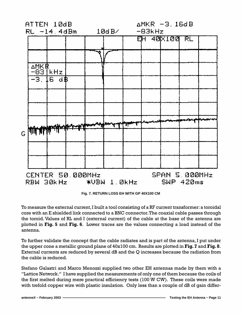
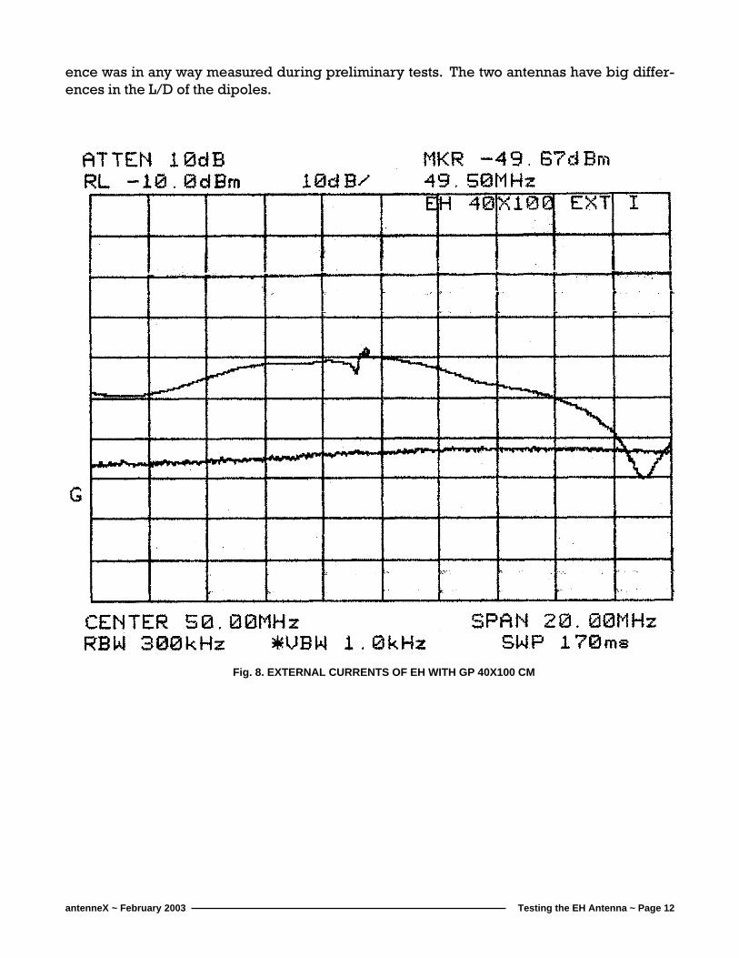
To further validate the concept that the cable radiates and is part of the antenna, I put underthe upper cone a metallic ground plane of 40x100 cm. Results are plotted in Fig. 7 and Fig. 8.External currents are reduced by several dB and the Q increases because the radiation fromthe cable is reduced.
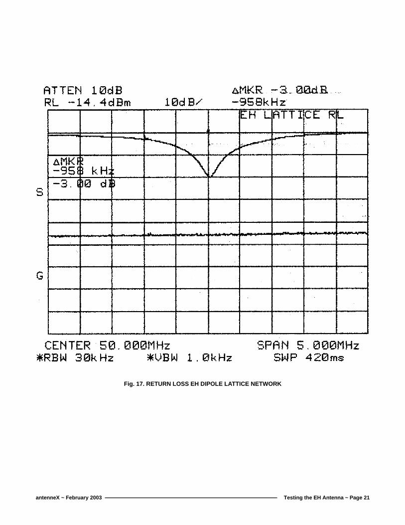
Stefano Galastri and Marco Menozzi supplied two other EH antennas made by them with a“Lattice Network.“ I have supplied the measurements of only one of them because the coils ofthe first melted during mere practical efficiency tests (100 W CW). These coils were madewith trefold copper wire with plastic insulation. Only less than a couple of dB of gain differ-
Fig. 7. RETURN LOSS EH WITH GP 40X100 CM
Testing the EH Antenna ~ Page 12antenneX ~ February 2003
ence was in any way measured during preliminary tests. The two antennas have big differ-ences in the L/D of the dipoles.
Fig. 8. EXTERNAL CURRENTS OF EH WITH GP 40X100 CM
Testing the EH Antenna ~ Page 13antenneX ~ February 2003
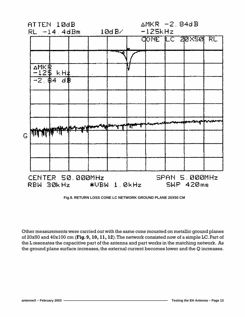
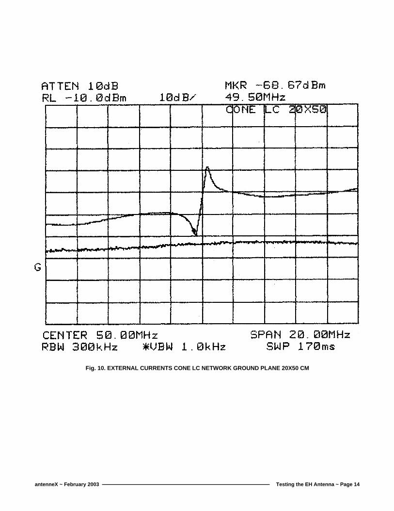
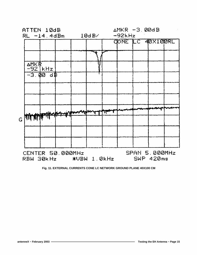
Other measurements were carried out with the same cone mounted on metallic ground planesof 20x50 and 40x100 cm (Fig. 9, 10, 11, 12). The network consisted now of a simple LC. Part ofthe L resonates the capacitive part of the antenna and part works in the matching network. Asthe ground plane surface increases, the external current becomes lower and the Q increases.
Fig.9. RETURN LOSS CONE LC NETWORK GROUND PLANE 20X50 CM
Testing the EH Antenna ~ Page 14antenneX ~ February 2003
Fig. 10. EXTERNAL CURRENTS CONE LC NETWORK GROUND PLANE 20X50 CM
Testing the EH Antenna ~ Page 15antenneX ~ February 2003
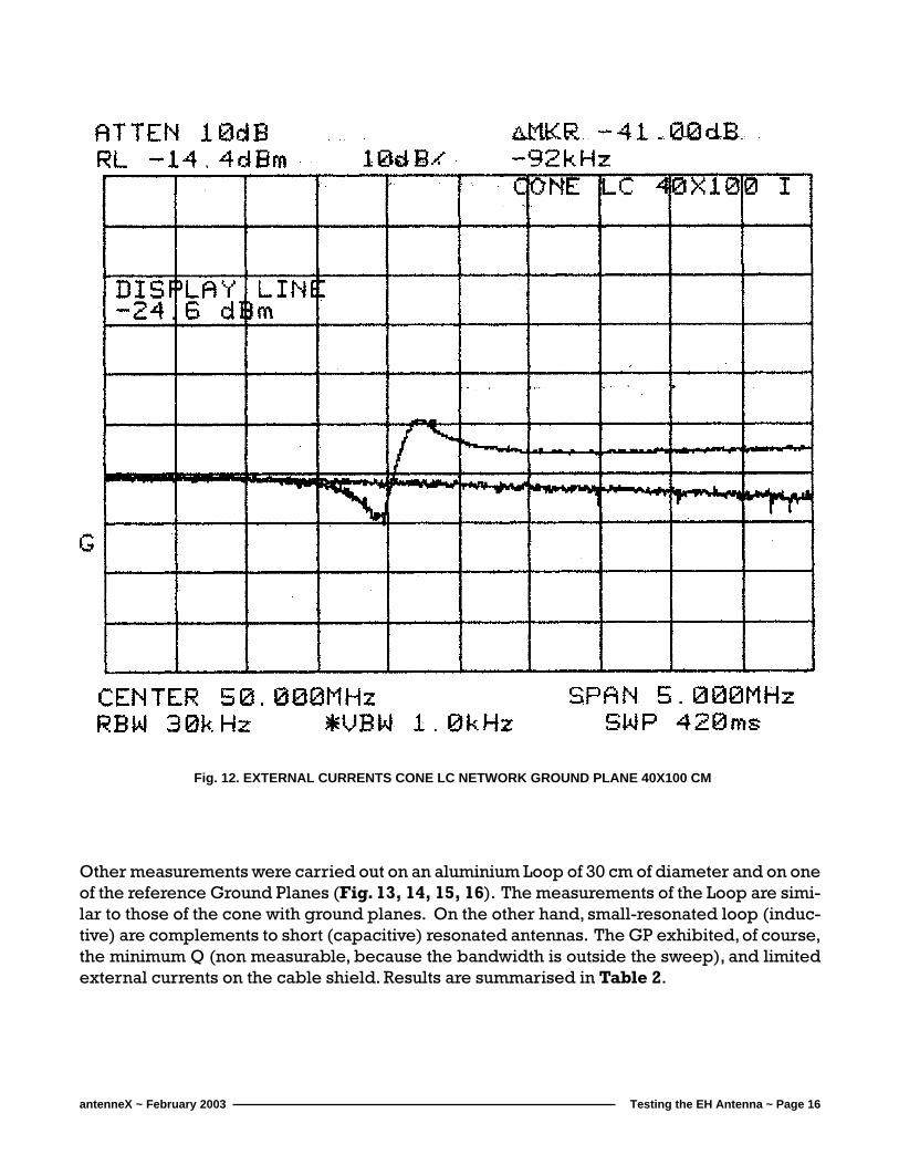
Fig. 11. EXTERNAL CURRENTS CONE LC NETWORK GROUND PLANE 40X100 CM
Testing the EH Antenna ~ Page 16antenneX ~ February 2003
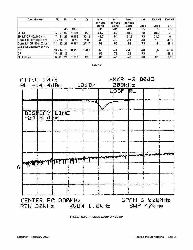
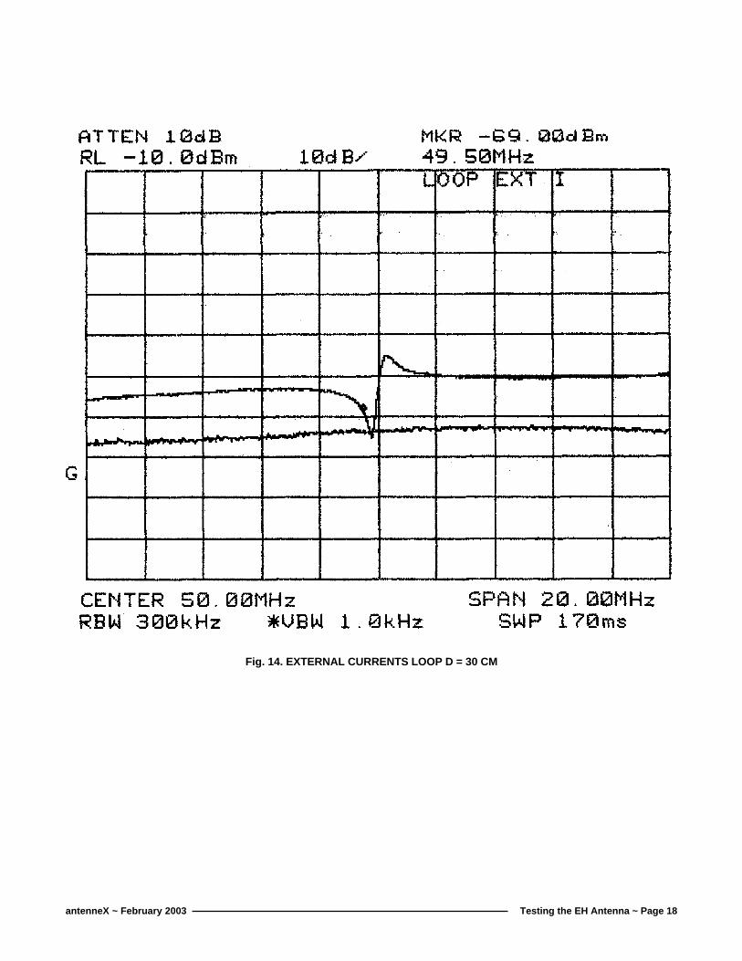
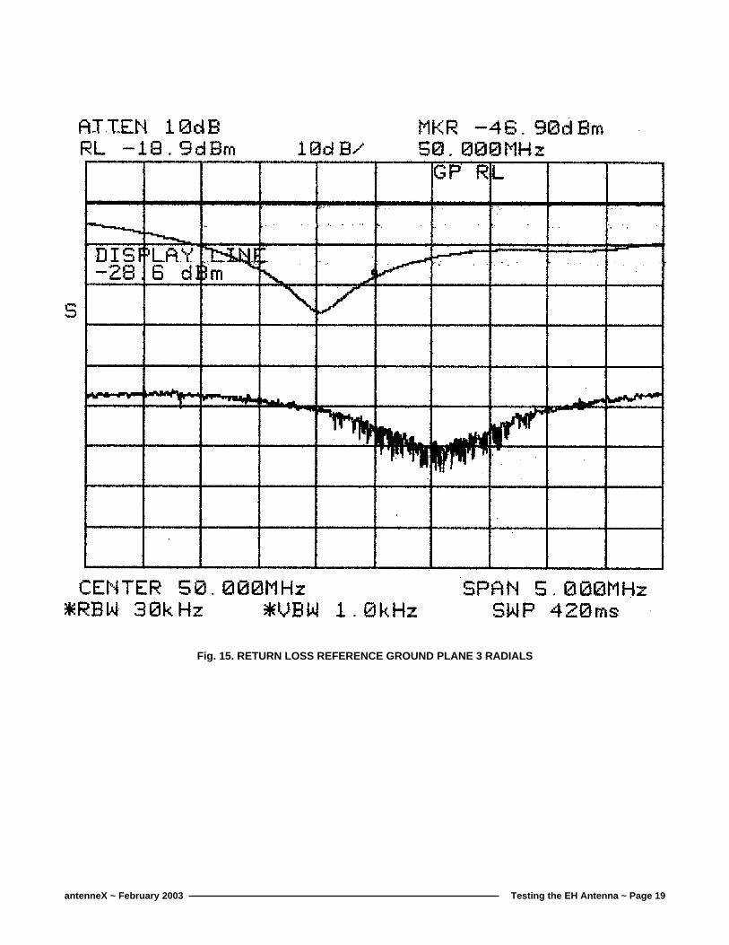
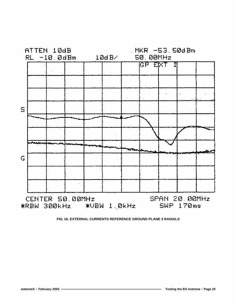
Other measurements were carried out on an aluminium Loop of 30 cm of diameter and on oneof the reference Ground Planes (Fig. 13, 14, 15, 16). The measurements of the Loop are simi-lar to those of the cone with ground planes. On the other hand, small-resonated loop (induc-tive) are complements to short (capacitive) resonated antennas. The GP exhibited, of course,the minimum Q (non measurable, because the bandwidth is outside the sweep), and limitedexternal currents on the cable shield. Results are summarised in Table 2.
Fig. 12. EXTERNAL CURRENTS CONE LC NETWORK GROUND PLANE 40X100 CM
Testing the EH Antenna ~ Page 17antenneX ~ February 2003
Fig.13. RETURN LOSS LOOP D = 30 CM
Table 2
Testing the EH Antenna ~ Page 18antenneX ~ February 2003
Fig. 14. EXTERNAL CURRENTS LOOP D = 30 CM
Testing the EH Antenna ~ Page 19antenneX ~ February 2003
Fig. 15. RETURN LOSS REFERENCE GROUND PLANE 3 RADIALS
Testing the EH Antenna ~ Page 20antenneX ~ February 2003
FIG. 16. EXTERNAL CURRENTS REFERENCE GROUND PLANE 3 RADIALS
Testing the EH Antenna ~ Page 21antenneX ~ February 2003
Fig. 17. RETURN LOSS EH DIPOLE LATTICE NETWORK
Testing the EH Antenna ~ Page 22antenneX ~ February 2003
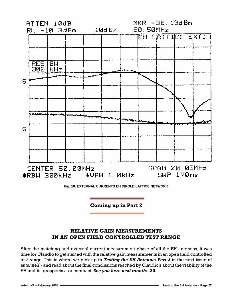
Fig. 18. EXTERNAL CURRENTS EH DIPOLE LATTICE NETWORK
Coming up in Part 2
RELATIVE GAIN MEASUREMENTSIN AN OPEN FIELD CONTROLLED TEST RANGE
After the matching and external current measurement phase of all the EH antennas, it wastime for Claudio to get started with the relative gain measurements in an open field controlledtest range. This is where we pick up in Testing the EH Antenna: Part 2 in the next issue ofantenneX - and read about the final conclusions reached by Claudio’s about the viability of theEH and its prospects as a compact. See you here next month! -30-

Testing the EH Antenna ~ Page 23antenneX ~ February 2003
BRIEF BIOGRAPHY OF THE AUTHORClaudio Re, I1RFQ is a graduate of Polytecnic of Turin in 1980with specialization in “Telecommunications andHyperfrequencies“. He is an owner of Sistel SRL and Sinfotel SRL,two small telecommunications, companies in Italy. He is also aconsultant and the Network Director of the World Family of RadioMaria, a Catholic Broadcasting Network that broadcasts now in27 different countries of the globe.
He has experimented with all kinds of equipment from 136 KHzto the optical frequencies (one-way communications at 22km)
Claudio was born in 1956, built his first crystal set receiver atage 6 and at 16, obtained his license with the callsign 1IRFQ.
antenneX Online Issue No. 70 — February 2003Send mail to [email protected] with questions or comments.
Copyright © 1988-2003 All rights reserved worldwide - antenneX©