Embed Size (px)
Citation preview
Centre de recherche sur l’emploi et les fluctuations économiques (CREFÉ) Center for Research on Economic Fluctuations and Employment (CREFE) Université du Québec à Montréal Cahier de recherche/Working Paper No. 143 Testing the Capital Asset Pricing Model Efficiently Under Elliptical Symmetry : A Semiparametric Approach Douglas J. Hodgson UQAM Oliver Linton London School of Economics Keith Vorkink Brigham Young University October 2001 Hodgson : Département des sciences économiques, Université du Québec à Montréal, C.P. 8888 Succursale Centre-Ville, Montréal, QC, Canada, H3C 3P8. Tel : 514-987-3000 (ext.4310). Email: [email protected]. Linton: Department of Economics, London School of Economics, Houghton Street, London WC2A 2AE, United Kingdom. Email: [email protected]. Vorkink: Marriott School of Management, Brigham Young University, Provo, UT, USA, 84602. Tel: 801-378-1765. Email: [email protected]. For their helpful comments, we would like to thank John Geweke and two referees, Pedro Gozalo, Gene Savin, and participants in seminars at Toronto, Montreal, McGill, and the 1998 summer meetings of the North American and European Econometric Societies. We also thank Eugene Choo and Roger Moon for research assistance and the National Science for financial support. Hodgson thanks CREST at INSEE for their hospitality while part of this research was being carried out.
Sommaire: Nous développons de nouveaux tests du modèle d’évaluation des actifs financiers (« CAPM ») qui tiennent compte de, et sont valides sous, l’hypothèse que les retours des actifs découlent d’un loi de probabilité elliptiquement symétrique. Cette hypothèse est nécessaire et suffisante pour la validité du CAPM. Notre test utilise un estimateur des paramètres du modèle qui a l’efficacité semiparamétrique quand on a un modèle de régression apparemment sans relation et qui a des erreurs qui suivent une loi elliptiquement symétrique. L’hypothèse de la symétrie elliptique nous permet d’éviter le problème d’estimer non-paramétriquement une fonction de haute dimension parce qu’on peut écrire la densité d’une loi elliptique comme une fonction d’une transformation unidimensionnelle de la variable aléatoire multidimensionnelle. La famille des lois elliptiquement symétriques inclue plusieurs lois leptokurtiques, donc elle est pertinente à des applications financières. Les bêtas obtenus avec notre estimateur sont plus bas que ceux qui sont obtenus en utilisant des moindres carrés, et sont moins compatibles avec le CAPM. Abstract: We develop new tests of the capital asset pricing model (CAPM) that take account of and are valid under the assumption that the distribution generating returns is elliptically symmetric; this assumption is necessary and sufficient for the validity of the CAPM. Our test is based on semiparametric efficient estimation procedures for a seemingly unrelated regression model where the multivariate error density is elliptically symmetric, but otherwise unrestricted. The elliptical symmetry assumption allows us to avert the curse of dimensionality problem that typically arises in multivariate semiparametric estimation procedures, because the multivariate elliptically symmetric density function can be written as a function of a scalar transformation of the observed multivariate data. The elliptically symmetric family includes a number of thick-tailed distributions and so is potentially relevant in financial applications. Our estimated betas are lower than the OLS estimates, and our parameter estimates are much less consistent with the CAPM restrictions than the corresponding OLS estimates. Keywords: Adaptive estimation, capital asset pricing model, elliptical symmetry, semiparametric efficiency. JEL classification: C22
1 Introduction
The mean-variance approach to asset pricing theory, initially investigated in work such as that ofTobin (1958) and Markowitz (1952, 1959), has great intuitive appeal and has the important practicaladvantage of greatly simplifying the modeling of asset returns. The principal result in this area isthe capital asset pricing model (CAPM) of Sharpe (1964), Lintner (1965), and Mossin (1966), whichposits that the expected excess return of any asset is linear in its covariance with the expected returnon the market portfolio.1 This relationship is formalized in the following equation:
E [Ri] = rf + ¯i (E [RM ]¡ rf ) ; (1)
where Ri is the random rate of return on asset i, ¯i = cov [Ri; RM] =var [RM ], RM is the rate ofreturn on the market portfolio and rf is the risk-free rate, which is assumed to be observed in theSharpe-Lintner version. De¯ning ri = E [Ri] ¡ rf ; equation (1) can be rewritten as ri = ¯irM:
The CAPM was originally derived under the assumption that either investors possess quadratic
utility functions or that asset returns are normally distributed. Since quadratic utility functions havethe intuitively unappealing property that they are decreasing at high consumption levels, the factthat the CAPM holds under normality for a much broader class of utility functions is comfortingto proponents of the model. Unfortunately, there is a considerable amount of evidence that theassumption of normality is not an appropriate one for asset returns. There is a voluminous literature(dating back at least as far as Fama (1963, 1965) and Mandelbrot (1963)) documenting the excessthickness of the tails in asset return distributions relative to the normal. This tail thickness isassociated with the tendency of asset returns to take values of extremely large magnitude withnonnegligible probability. Thus, it seems that we would need to fall back on the assumption ofquadratic utility to justify the CAPM relationship (1). However, it has been shown that although, inthe absence of strong restrictions on investor preferences, the assumption of normality is su±cient togenerate (1), it is not necessary. In particular, Chamberlain (1983), Owen and Rabinovitch (1983),and most recently Berk (1997) show that (1) can be obtained under the assumption of ellipticallysymmetric return distributions without the strongly restricting preferences.2 Berk (1997) shows thatelliptical distributions are the most general distributional assumption that will imply the CAPMwhen agents maximize expected utility, that is, elliptical symmetry is both necessary and su±cientfor the CAPM. The elliptically symmetric family contains the Gaussian distribution as a special case,but many well-known thick-tailed distributions also belong to this class - the Student t, logistic, andscale mixed-normal being examples.3
1The market portfolio is a value weighted portfolio of all assets in the market.2See also Ingersoll (1987).3See Fern¶andez, Osiewalski, and Steel (1995) for some generalizations of ellyptical symmetry that are interesting
3
That asset returns may be non-normal can have important implications for the econometricimplementation of the model, which often involves the estimation of a system of linear equationsspeci¯ed as a seemingly unrelated regressions (SUR) model (see, for example, MacKinlay (1987) andGibbons, Ross, and Shanken (1989)). The standard estimator of this model is ordinary least squares(OLS), which will be fully e±cient under normality, but will not be fully e±cient if normality fails.In an innovative paper, Zhou (1993) considers implementation of OLS under possible non-normality,deriving a procedure to correct the size problems that may occur in CAPM tests if returns are
elliptical but non-normal.The contribution of the present paper is to derive an estimator of the SUR model that will be
fully e±cient in the presence of elliptical symmetry of general form. The resulting estimator will bemore e±cient than OLS and will yield more powerful CAPM tests than those of Zhou (1993) forexample. The estimator we propose is semiparametric in nature, treating the true distribution ofthe data as being unknown (aside from the elliptical symmetry restriction) and is fully \adaptive"(Bickel (1982)), i.e., it will achieve the same asymptotic covariance matrix lower bound as would themaximum likelihood estimator if the distribution of the data were known.
Semiparametric methods such as we develop here employ nonparametric kernel smoothers to es-timate the unknown distribution of the data and are well developed for single equation estimationproblems, see for example Stone (1975), Bickel (1982), and Kreiss (1987). Some methods have alsobeen proposed for multivariate data, see Bickel (1982) and Hodgson (1998b). However, there areproblems with smoothing methods with high dimensional data: the estimates are hard to plot andinterpret, and have slow convergence rates. For this reason, some intermediate structures are be-coming increasingly popular, such as additive models in regression, see for example Horowitz (2001).This problem is often referred to as the \curse of dimensionality" and is of particular relevance to ourproblem of e±ciently estimating the SUR system, since the semiparametric estimator requires thekernel estimation of a density whose dimensionality equals that of the system. However, if we exploitthe elliptical symmetry assumption underlying the CAPM, then we have the opportunity to avoidthe curse of dimensionality. This is because the density function of a vector-valued elliptical randomvariable can always be rewritten as the density function of a scalar random variable, regardless ofthe dimension of the vector. Owen and Rabinovitch (1983), in showing that the CAPM would holdunder elliptical symmetry, also suggested that the possibility of elliptical symmetry should be takeninto account in the formulation of econometric models of the CAPM. In recent years, it has becomepossible, due to some advances in econometric estimation theory, to incorporate the general assump-
tion of elliptical symmetry into an econometric model without having to be more speci¯c about theactual functional form of the distribution. The implication is that our computation of an adaptivefrom statistical point of view.
4
estimator will always only require a one-dimensional nonparametric estimation problem, regardlessof the size of the system, and so is not subject to the curse of dimensionality. This intuition is shownto be correct by Stute and Werner (1991).
In Section 2, we introduce the SUR model that we are interested in analyzing. In Section 3, weoutline a formula for computing an adaptive estimator and give its asymptotic properties. Section 4reports the results of our empirical test of the CAPM, while Section 5 investigates the performance ofthe estimator through a Monte Carlo simulation analysis. A mathematical appendix contains proofs.
We use kAk =¡trATA
¢1=2 to denote the Euclidean norm of a vector or matrix A, while P! denotesconvergence in probability and D! denotes convergence in distribution:
2 The SUR Model
In this section we consider the speci¯cation and estimation of a general seemingly unrelated re-gressions (SUR) model. The CAPM regression, implemented in Section 4, falls within this class.Consider the m-equation seemingly unrelated regression model
yt = ®+ xt¯ + ut := wtµ + ut; t = 1; : : : ; n; (2)
where yt 2 Rm, ® 2 Rm; wt = [Im xt] ; in which
xt =
2666664
x1t 0x2t
. . .
0 xmt
3777775; ¯ =
2664
¯1...¯m
3775 ; ut =
0BB@
u1t...umt
1CCA ;
where xit 2 Rki and ¯i 2 Rki for every i = 1; : : : ;m; the full parameter vector is µ =£®T ; ¯T
¤T 2Rm+k; where k = k1 + ¢ ¢ ¢ + km: The error terms ut 2 Rm are i.i.d., mean zero innovations withE(utuTt ) = §u: Here, the regressors xt are assumed to be stationary and ergodic, and we assumethat xt and ut are independent (i.e., that the regressors are strictly exogenous). The asymptoticproperties of least squares estimators are standard under these assumptions.
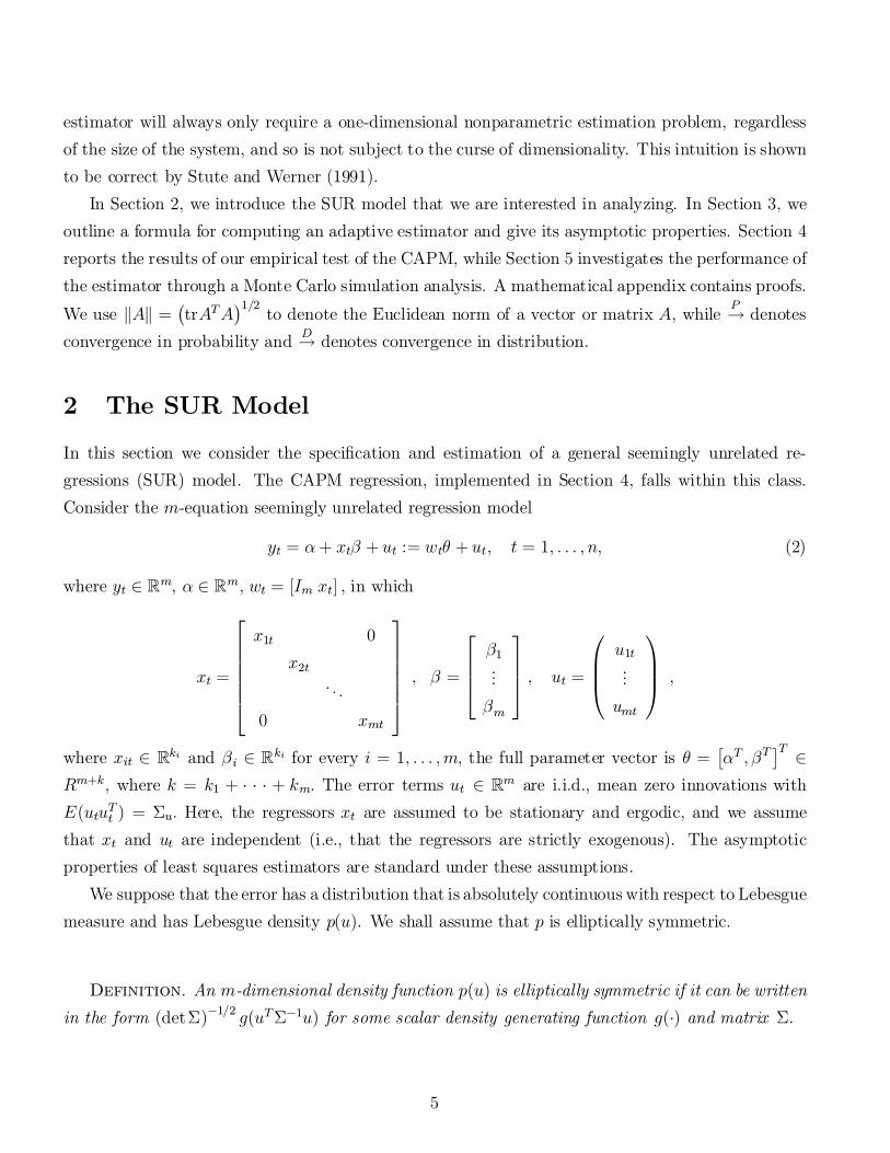
We suppose that the error has a distribution that is absolutely continuous with respect to Lebesguemeasure and has Lebesgue density p(u). We shall assume that p is elliptically symmetric.
Definition. An m-dimensional density function p(u) is elliptically symmetric if it can be writtenin the form (det§)¡1=2 g(uT§¡1u) for some scalar density generating function g(¢) and matrix §.
5
The practical content of the elliptical symmetry restriction arises from the fact that the function ghas only a scalar argument. Note that the matrix § is identi¯ed only up to a scalar multiple, as scaletransformations in § can be incorporated into the function g. Without loss of generality, we shall usethe normalization det (§) = 1: Under this normalization; § is proportional to the covariance matrixof u, which we denote by §u, so that §u = c§, where c = (det §u)1=m, i.e., § = §u=(det §u)1=m
[c.f. Kelker (1970) and Stute and Werner (1991)]. Also worth noting is the fact that the informationmatrix of p, p, is proportional to the inverses of these matrices [c.f. Mitchell (1989)].
If p were known, the log-likelihood for the data would be
Ln(µ) =nX
t=1
ln p(yt ¡ wtµ);
and a standard estimation method is to choose µ to maximize Ln(µ): One estimation strategy whichavoids complicated nonlinear optimization associated with non-Gaussian p; is to use a two-stepNewton-Raphson estimator µ starting from a preliminary
pn-consistent estimator bµ that was ob-
tained from the Gaussian likelihood (OLS, for example). This approach to estimation apparentlyoriginates with R.A. Fisher and has been widely used in econometrics. Under general conditions,this will be ¯rst order asymptotically equivalent to the maximum likelihood estimator (MLE), i.e.,
pn(µ ¡ µ0) D! N(0; I¡1);
where the asymptotic information matrix I is such that n¡1 (@2Ln (µ0) =@µ@µ0)P! I. In order to
derive an expression for I, we de¯ne '(u) = p0(u)=p(u); the m-dimensional score vector of p, andp =
R'(u)'(u)Tp(u)du, the information matrix of p. The asymptotic information matrix is
I =
"p E [pxt]
E£xTt p
¤E
£xTt pxt
¤#:
We use a Newton-Raphson iterative approach to estimation butmust replace the unknown densityp by a nonparametric estimator; thus our adaptive estimator eµ will have the form
eµ = bµ + bI¡1n (bµ)b¢n(bµ); (3)
where b¢n and bIn are estimates of the ¯rst and second standardized derivatives of Ln respectively.Their computation is described in Section 3 below. In particular,
b¢n(bµ) = ¡1n
nX
t=1
wTt b't(but);
where b't(but) is a consistent estimator of the m-dimensional score vector '(ut); while but = yt ¡ wtbµ.The standard approach to this problem is to use multivariate kernel estimates bp and bp0 to construct
6
b'; with some observations possibly being trimmed, see Bickel (1982). Unfortunately, if m is largesuch estimates will have poor performance due to the curse of dimensionality, see HÄardle and Linton(1994). We show how to construct a b't(:) that takes advantage of our elliptical symmetry assumptionand employs only one-dimensional smoothing operations.4
3 Estimation
The formula for an adaptive estimator given in (3) above presupposed the existence of consistentscore and information estimators b't and bIn. In this section, we provide an algorithm for computingnonparametric estimates of these quantities while imposing the restriction that the errors futg have anelliptically symmetric distribution. Recall that the elliptical symmetry assumption allows us to reducethe dimensionality m of the density p (u) to the dimension one of the function g
¡uT§¡1u
¢= g
¡"T "
¢,
where " = §¡1=2u is a spherically symmetric random variable with density f (") = g¡"T "
¢= g (v)
where v = "T ": We can thus obtain an indirect estimate of the density of u from a direct estimateof the density of the scalar random variable v: It may be preferable for computational reasons to
directly estimate the density of the random variable z = ¿ (v), rather than that of v itself, and inour theory we allow for estimation of a general Box-Cox (1964) transformation ¿ (v) = (v³ ¡ 1)=³:We discuss our choice of ³ in our empirical and simulation work below. We will use direct kernelestimates of the density of z, denoted by °(z); to indirectly obtain consistent estimates of the scoreand information of p. By Theorem 2.1.2 of Casella and Berger (1990) we have
°(z) = h(¿¡1(z)) ¢¯¯@¿¡1(z)@z
¯¯ = cm
£¿¡1(z)
¤m=2¡1 g(¿¡1(z)) ¢ J¿(z);
where h(v) = cmvm=2¡1g(v) with cm = ¼m=2=¡(m=2) is the density of v, see Muirhead (1982), whileJ¿(z) = j@¿¡1(z)=@zj: Thus, g(v) = c¡1m J¡1¿ (¿(v))v1¡m=2°(¿ (v)): This gives us our desired expressionfor g(v) - and hence for f(") and p(u) - in terms of ° (z).
Our algorithm for estimating ' and I proceeds according to the following steps:
Step 1: First obtain bµ (by ordinary least squares, for example) and de¯ne the associated OLSresiduals fbutgnt=1 and the standardized residuals fb"tgnt=1, where b"t = b§¡1=2but, b§ = bc¡1b§u,b§u = (n¡ k ¡m)¡1 Pn
t=1 butbuTt , and bc = [det b§u]1=m: Then compute the univariate transformedsequence fbztgnt=1, where bzt = ¿(bvt) with bvt = b"Tt b"t:
4As shown in Stute and Werner (1991) these procedures ensure density estimators whose pointwise rate of conver-gence is the one-dimensional rate.
7
Step 2: Compute leave-one-out kernel density and derivative estimators using data fbztg; kernelKhn(¢); and bandwidth hn:
b°t(z) =1n¡ 1
nX
s=1s 6=t
Khn (z ¡ bzs) ; b°0t(z) =1n¡ 1
nX
s=1s6=t
K0hn(z ¡ bzs):
Step 3: Introduce the following trimming conditions: (i) b°t(bzt) ¸ dn; (ii) jbztj · en; (iii) j¸(bzt)j · bn;(iv) j½1=2(bzt)b°0t(bzt)j · cnb°t(bzt); where ½(z) = v¿ 0(v)J¡1¿ (z) [recall that v = ¿¡1(z)] and ¸(z) =(d=dz)¡1½1=2(z).5 Then estimate the score and information of p(u) as follows:
b't(but) =
8<:
b§¡1=2b"ths(bvt) + ¿ 0(bvt) b°0t
b°t (bzt)i
if (i)¡ (iv) all hold
0 otherwise;
where s(v) = (1¡m=2)v¡1 ¡ J0¿J¿
f¿ (v)g ¿ 0(v) and bp = 1n
Pnt=1 b't(but)b't(but)T :
Step 4: Then de¯ne the score and information estimators for the model as
b¢n(bµ) = ¡ 1n
nX
t=1
wTt b't(but) ; bIn(bµ) =1n
nX
t=1
wTt bpwtn¡1; (4)
and compute the adaptive estimator eµ given in (3) above.
The important point to notice about this estimator is that it employs a direct kernel estimate ofthe density of the univariate process fztg in order to arrive at score and information estimates ofthe multivariate process futg.
We now state the main result of the paper, which is proved in the Appendix:
Theorem 1 Suppose that p is ¯nite and positive de¯nite, thatR10 v
m=2s(v)2g(v)dv < 1, that theerror distribution is absolutely continuous with respect to Lebesgue measure with Lebesgue density
5These trimming conditions ensure consistency of our score estimator when a Gaussian kernel is being used, i.e.,
when Khn is a Gaussian kernel. For other kernels often employed in the literature [e.g., Schick's (1987) logistic kernel
and the bi-quartic kernel], the necessary trimming conditions, if they di®ered at all from these, would be less stringent,so that these conditions will still be su±cient for consistency but may not be necessary. Simulation work reported by
Hsieh and Manski (1987) and Hodgson (1998a) ¯nds that, for a Gaussian kernel, the adaptive point estimate is not
very sensitive to variation in the value of the trimming parameters, and that good results are obtained in practicewhen we trim as little as 1% of the observations.
8
p(u), that the regressors xt are strictly exogenous, and that the constants in (i)-(iv) satisfy cn ! 1,en ! 1, bn ! 1, hn ! 0, dn ! 0, hncn ! 0, enh¡3n = o(n), and bnh¡3n = o(n). Then,
pn(eµ¡ µ) D! N (0; I¡1); (5)
i.e., the estimator eµ is adaptive.
Remarks. (a) The moment conditionR10 v
m=2s(v)2g(v)dv < 1 is potentially restrictive; itsimplications for the moments of u will depend on the transformation ¿ (¢). For example, when thetransformation is ¿(v) = (v³ ¡ 1)=³ with either ³ = 0; ³ = 1; or 1=2m, the condition impliesE [
¡"T"
¢m=2¡2] < 1:However, when ³ = m=2; there is no restriction on the moments of u.(b) Note that the information matrix estimator bIn(bµ) de¯ned in (4) is a consistent estimator
of the asymptotic covariance matrix, so that bIn(bµ) ¡ I = op(1): We can therefore use bIn(bµ) inthe construction of t-ratios and Wald statistics which will have respective standard normal and
chi-squared asymptotic distributions. Let µ` and eµ` be the `th elements of the µ and eµ vectors,respectively. Now suppose we wish to test the null hypothesis that µ` = c, where c is some constant.Then we can compute the usual t-ratio, as follows:
t =
pn
³eµ` ¡ c
´
r³bI¡1n (bµ)
´``
;
where³bI¡1n (bµ)
´`
is the `th elements along the diagonal of bI¡1n (bµ). Under the null hypothesis,
t D! N (0; 1) : If we want to test the joint hypothesis ¿ (µ) = 0, where ¿ is a known (m+k)£ 1 vectorof functions, we can compute the Wald statistic
W = n¿ (eµ)0h ¢¿(bµ)bI¡1n (bµ) ¢¿(bµ)0
i¡1¿ (eµ)0;
where ¢¿ is the matrix of derivatives of ¿ with respect to µ: Under the null hypothesis W D! Â2m+k:(c) Our estimator of the information matrix, although consistent, has a ¯nite sample upwards
bias that therefore biases downwards our standard error estimates. In our empirical application,we employ a simple degrees of freedom correction. Write b°0t =
Ps !
0nts and b°t =
Ps!nts for some
weights ! 0nts and !nts implicitly de¯ned in our estimation algorithm. We replace (b°0t)2 and (b°t)2 in(4) by (b°0t)2 ¡ P
s(!0nts)2 and (b°t)2 ¡ P
s(!nts)2 respectively. The correction terms
Ps(!
0nts)2 and
Ps(!nts)2 consistently estimate the degrees of freedom bias terms (see Linton (1995)).(d) We employ one-dimensional kernel estimates of the transformed variable z, which has a
support restriction of z ¸ 0: The kernel estimate will generally have a downward bias in the right
9
neighborhood of zero. This bias arises because for points close to zero, the kernel smoother assignspositive weight extends to points x · 0 where f(x) = 0: The over°ow in weights beyond the lowersupport of 0 can be corrected by applying a result of Schuster (1985), who o®ers a correction thatincorporates this over°ow to the region z < c, for ¯nite c, back into the region z ¸ c by adding amirror image term n¡1h¡1n K((z ¡ 2c+ zi)=hn) to n¡1h¡1n K((z ¡ zi)=hn): The resulting estimator forz ¸ c is given by
efn(z) =1nhn
nX
i=1
·K
µz ¡ zihn
¶+K
µz ¡ 2c+ zihn
¶¸:
In our case, c = 0: Schuster (1985) also proves consistency and asymptotic normality results for thisestimator.
(e) The advantage of the adaptive estimator over alternative estimators such as OLS is that, in thepresence of thick-tailed errors, it will downweight outliers in an optimal manner, °exibly adaptingto the tail behavior of the sample through the nonparametric score estimator. If the regressiondisturbances are not i.i.d., but have an unconditional distribution whose thick tails are induced byconditional heteroskedasticity, then an extension of results of Hodgson (2000) to our model shouldbe possible if the regressors are strictly exogenous and the disturbances are uncorrelated with anelliptical unconditional density. Our nonparametric score estimator will consistently estimate thescore of this unconditional error density and the distribution theory outlined above should follow,with the standard errors being asymptotically correct.
4 Empirical CAPM Tests
4.1 Background
There is an extensive empirical literature on the CAPM, with important early work by Black, Jensen,and Scholes (1972) and Fama and MacBeth (1973).6 More recent work has employed the multivariateregression model introduced above, for example Gibbons (1982) and Stambaugh (1982). Estimatingthe model for m portfolios over a sample of length n; we have:
rt = ® + ¯rM;t + ut; t = 1; : : : ; n; (7)
where rt is the m-vector of portfolio excess returns; ® and ¯ are m-dimensional parameter vectors;rM;t is the excess market return, and ut is an m-vector of disturbances. If there is some systematiccomponent of returns that is not due to market risk exposure, it will appear in the intercept (®). If
6See Campbell, Lo, and MacKinlay (1997) for a more comprehensive discussion of empirical tests of the CAPM.
10
the CAPM holds, then ® = 0, but the existence of additional returns implies ® 6= 0. The followingnull hypothesis on the parameters of (7)
H0 : ®i = 0 i = 1; : : : ;m; (8)
implies that no signi¯cant excess returns are present that cannot be explained by variation in themarket return. We test this hypothesis by constructing a standard Wald test
J = ~®0 [cvar(~®)]¡1 ~®;
where ~® is an estimate of ® and cvar(~®) estimates the asymptotic covariance matrix of ~®:7 Alterna-tively, one could test for the signi¯cance of additional regressors in (7). For example, Basu (1977)considers price-earnings ratios, Banz (1981) includes market size, and Fama and French (1992, 1993)consider a ¯rm's book value to market value ratio as well as size.
4.2 Elliptically Symmetric Returns: Adaptive Estimation and Tests
In applying our estimator, some care should be taken regarding the possibility of conditional het-eroskedasticity in the regression disturbances. The CAPM is derived under the assumption of el-liptical symmetry in asset returns, which implies that the disturbances may possess conditionalheteroskedasticity and higher order dependence with the regressors. The presence of conditional het-eroskedasticity implies that some problems exist with both OLS and our estimator. In the case ofOLS, the standard errors will be biased (Van Praag and Wesselman (1989)). Our semiparametricestimator loses its adaptivity property if there is high order dependence between ut and rM;t: Wediscuss some remedies below.
First, a parametric model of the conditional heteroskedasticity can be introduced into the modeland estimation procedure. The parameter vector (µ) can be expanded to include the conditional het-eroskedasticity model and estimation can proceed as in the previous section. However, in the context
of regression models where second moments appear in the mean equation via `¯' the distributiontheory of the estimator is much more di±cult. Hodgson and Vorkink (2001) develop a semipara-metric estimator for a multivariate GARCH-in-mean model such as that of Bollerslev, Engle, andWooldridge (1988).
A second solution would be to use a procedure as proposed by White (1980) and correct for theconditional heteroskedasticity in the preliminary estimation step. This should purge any high orderdependence between rM;t and ut allowing the estimation theory as discussed in the previous sectionto be valid. A model for the conditional heteroskedasticity is required at the preliminary estimation
7See MacKinlay (1987) and Gibbons, Ross, and Shanken (1989) for a discussion of CAPM tests along these lines.
11
stage. We could proceed nonparametrically, estimating the conditional variance of equation i, fori = 1; : : : ;m; by taking the squares of the residuals from the preliminary regression u2i;t and usingkernels locally regress them on the contemporaneous market excess return (rM;t) as de¯ned below:
¾2i (rM;t) =Pni=1K(rM;t¡rM;ihn
)u2iPni=1K( rM;t¡rM;ihn
); (9)
where K(:) is a kernel weighting function and hn is a bandwidth. We could then use rwi;t = rt¾i;t
and estimate the model using©rwi;t
ªnt=1
. Multivariate normality tests on the series frwi;tg ¯nd excesskurtosis to be present (see below), implying that normality assumptions are not appropriate evenafter accounting for conditional heteroskedasticity. Alternatively, one could proceed parametricallyby specifying the GARCH(1,1) model:
¾2i;t = ai;0 + ai;1¾2i;t + ai;2u2i;t:
One approach to correcting for the bias present in the OLS standard errors is to use informationfrom the unconditional distribution to correct for the conditional heteroskedasticity. As was notedearlier, if second moments are allowed to vary then the unconditional distribution will be thick-tailed.The degree of kurtosis in the unconditional distribution can be used to adjust variances as describedin Zhou (1993), who shows that a simple correction of the Wald statistic will generalize it to allowelliptical returns, as follows:
J¤ = J ¢ ´¡1 D! Â2N ;
where J is the standard Wald statistic, ´ = 1+·x=(m(m+2)); and ·x is Mardia's (1970) multivariatemeasure of kurtosis. Undermultivariate normality, À = 0 and J¤ = J . However, when excess kurtosisexists, À > 1 and J¤ < J:
4.3 Results
We use daily data on stock returns taken from the CRSP ¯les and running from January 1996 toDecember 1997.8 We construct three portfolios by sorting ¯rms according to size (market value).On each trading day ¯rms are placed into quartiles according to the NYSE ¯rm size. Daily value-weighted returns are then constructed for the ¯rms in each of the ¯rst three quartiles.9 Our use ofdaily data is a bit unusual, but the CAPM itself says nothing about the length of the return period,and the question as to how well daily returns are approximated by the mean-variance model seemsto us to be of no less intrinsic interest than the same question applied to monthly or annual returns,
8Firms that are traded on the NYSE, NASDAQ and AMEX are included.9We exclude the largest quartile because of its similarity to our measure of the market.
12
for example. Daily returns tend to be more highly non-normal than returns over longer intervals(although some degree of non-normality is present even there), suggesting that our econometricmethodology is particularly well suited to this question.10 Applications to weekly and monthly datawill be pursued in future work.
Tables I and II provide the summary statistics for the risk-free rate (30 day T-bill rate) rf;t, theannualized return on the CRSP value-weighted market portfolio rM;t, and annualized portfolio excessreturns rt ¡ rf;t: Multivariate normality is rejected using either the univariate kurtosis estimates or
the Jarque-Bera (1980) tests performed on the individual series reported in Table I. The multivariatemeasures of kurtosis also reject normality as seen in Panel A of Table II. Panel B shows that Beran's(1979) test of elliptical symmetry fails to reject at the 10% level the null that excess returns are el-liptical. We also consider returns weighted by estimated conditional standard deviations. Normalityis rejected on either set of returns, although those weighted nonparametrically have smaller kurtosis.In fact, for the size 3 portfolio, the Jarque-Bera test fails to reject. However, when we look at themultivariate tests, normality is strongly rejected while elliptical symmetry is not rejected, for boththe parametric and nonparametric conditional heteroskedasticity estimates.11
Table III reports the results of estimating (7) using unweighted returns. The OLS estimates of ¯are positive and of ® are close to zero (relative to their standard errors). The adaptive estimates arecomputed using a Gaussian kernel with Schuster's (1985) correction and the Box-Cox transformationz = ¿ (v) =
¡v³ ¡ 1
¢=³; with ³ = 1=2m:12 We choose our bandwidth parameter by using separate
optimal MISE rule-of-thumb (Silverman (1986)) bandwidths for ° (z) and °0 (z), respectively. Ingeneral, we ¯nd that the point estimates of ® (¯) using the adaptive estimator are greater (lesser)than their OLS counterparts. Some of the di®erences in the point estimates are substantial. Forexample, the adaptive method estimates that the unexplained return in the size 1 portfolio returnswill be at least 12% while the OLS estimates are about 5%. The di®erence in standard errors betweenthe adaptive procedures and the Gaussian methods is substantial. The reduction is 15% on averagefor the adaptive estimates. These e±ciency gains also appear in the simulation study reported below.
Tables IV and V report the results of estimating (7) using the nonparametric and the GARCH(1,1)weighted returns, respectively. As in the unweighted return regression, we obtain estimates of ®
10Unconditional GMM estimation of the model would use the moment conditions E [ut ] = 0 and E [utrM;t ] = 0,
leading to the OLS point estimates, with possibly di®erent standard errors. The resulting Wald statistic would have alack of power similar to that of the OLS Wald statistic, due to the sensitivity of the estimator to thick tails in return
distributions.11Bollerslev (1987) and Nelson (1991) also ¯nd signi¯cant nonnormalities in GARCH standardized distributions.12This transformation provided good results in Monte Carlo experiments (not reported) and increases smoothing
as the dimension increases, with the limit as m ! 1 being the natural log transformation. This increased smoothing
reduces the bias of the nonparametric estimate as the dimension increases.
13
that are larger, and of ¯ that are smaller, with the adaptive estimation than with OLS. We also ¯ndthat estimates of ¯ are lower using the adaptive method relative to OLS. The results suggest a returnmodel that places less weight on market variation and more weight on additional factors. Standarderrors again decline using the adaptive estimator, with the reduction being 11% on average.
We report Wald statistics of the zero-intercept null in Table VI. For the unweighted returns we¯nd that none of the estimation methods lead to a rejection at the 10% level, although the adaptiveestimator has a p-value only slightly greater than 0.10, as opposed to the OLS the p-value of 0.89
(the latter includes the Zhou (1993) correction). The adaptive estimator suggests the presence of asize (market value) e®ect on returns. The ine±cient OLS estimator lacks su±cient power to rejectthe model, even in the presence of weighted returns. Table VI shows that, for both sets of weightedreturns, OLS cannot reject while the adaptive estimator strongly rejects, with p-values less than0.01.
Our results suggest the use of an alternative model of returns. Our results lend support to theuse of a multi-factor model, possibly incorporating the market size of a ¯rm. We ¯nd that ¯rms withsmall market capitalizations earn excess returns relative to the CAPM predictions. Our estimatormeasures these excess returns to be substantially higher than OLS estimates, with the di®erence aslarge as 7% annually for ¯rms in the smallest quartile.
5 Simulation Analysis
We now investigate the ¯nite sample size and power properties of the Wald tests computed with thedi®erent estimators. We employ Davidson and MacKinnon's (1998) graphic method of comparingp-value plots and power-size plots. A large number of realizations of a given test statistic J arecomputed from data sets generated under the null and under a speci¯ed alternative hypothesis. Welabel the Wald statistics computed from the adaptive estimator and OLS as J and JOLS respectively.
Step 1: In generating our simulated data sets, each return ·ri;t is constructed by taking the productof the market return rM;t and the estimated beta ^
i; and adding a randomly selected residual fromsome prespeci¯ed distribution,
·ri;t = ®h+ ^irM;t + ui;t:
The distributions from which we draw ui;t are Student twith 3 degrees of freedom, twomixed normals,and normal. To compute the mixed normals, de¯ne the uniform random variable U 2 [0; 1] : IfU < (1¡ ²), then let ut =
p·1zm. Otherwise, we let ut =p·2zm. The resulting ut will follow
a mixed normal distribution. We set ² = :8; ·1 = 0:65 (MN1) ; or 0:45 (MN2) and ·2 = 6 in the
14
simulations.13 The intercept is set to ®h = 0 or ®h = :05, the latter being the approximate averageabsolute intercept from the empirical data. We use the same residual in constructing both thealternative and null series.
Step 2: For both the null and alternative data sets estimate the above model and then computeJ and the p-value under the null distribution for each statistic. The Gaussian kernel was used inconstructing the adaptive estimates. The p-value for the statistic constructed using the alternativedata set also uses the null distribution to obtain the p-value.
Step 3: Repeat Steps 1 and 2 many times. We chose to simulate the data and statistics 1,000times which should provide reasonable accuracy in the p-values we report.
Step 4: Given the simulated test statistics and their associated p-values, then calculate theempirical distribution function of the p-values generated by each statistic. This is obtained in thefollowing manner. Recall that the p-value of a statistic $j is the probability of observing a value ofthe statistic more extreme than $j: Let F (xi) represent the estimate of the c.d.f. of the p-valuesgenerated by a given statistic at the point xi and de¯ne p($j) to be the p-value associated withstatistic $j. Then F (xi) is calculated using the following formula:
F (xi) =1W
WX
j=1
I (p($j) > xi) ;
where W is the number of simulations and I is an indicator function that is equal to one if theargument is true and zero otherwise. To generate F (xi) ; it is recommended that a grid of valueslying in the interval between 0 and 1 be chosen to save time and computer storage space. We chosethe grid (X) to be the following: X = f0:001; 0:002; 0:003; : : : ; 1g and obtained the associated F (X)for all statistics under both the null and alternative.
Once the empirical distributions of each statistic are generated they can be graphed to comparethe size and power properties of the statistics. To compare size properties the following graph,entitled a p-value plot, is recommended. The plot is constructed by graphing of Xi versus F (Xi) foreach of the statistics. A test with appropriate size would follow the 45± since this is the c.d.f. of anyp-value distribution. When the graph is above (below) the 45± line the associated statistic is over(under) rejecting the null hypothesis.
To compare the power of two given test statistics, Davidson and MacKinnon (1998) recommendthe graph entitled power-size plot. The power-size plots graph F a (Xi) against Fn (Xi) where thesestand for the empirical distributions of the p-values from a test statistic under the alternative andnull respectively. When this line is plotted for a competing statistics any deviant size propertiesare removed by graphing F n (Xi) on the x -axis. Because the actual size is used as the x -variable,
13We scale the errors so that their variances match those in our empirical data.
15
di®erences in power cannot be attributed to di®erences in size between two competing statistics.
Size The simulations indicate that the tests constructed with our estimator are, in general, well-sized. However, this is not true in all cases. We list the results of our simulations in the p-valueplots in Figures 1, 3, and 5. In some cases the method appears to be undersized (normality, m = 4;MN2, m = 4). It appears that as the dimension increases the size of the adaptive tests declines.This could be due to our transformation choice and could potentially be corrected by ¯ne-tuning ourselection method.
Power Power results are reported in Figures 2, 4, 6, and 7. For all the simulations using thick-tailed distributions, the adaptive estimator leads to more frequent rejections than OLS with theincrease as great as 79% in one case (MN1; m = 4). The power appears to increase with dimension(m) as seen in the Figures 2, 4, and 6. The adaptive estimator is less powerful if the errors actuallyare normal.
A Appendix
A.1 Proof of Theorem 1
To prove the adaptivity of eµ we must establish the following two convergence results:
b¢n(bµ) ¡ ¢n(bµ) P! 0; (A.1)
andbI(bµ) ¡ I P! 0; (A.2)
where ¢n(bµ) = ¡n¡1 Pnt=1wTt '(but). We can use arguments analogous to those of Bickel (1982),
Linton (1993, p. 566), or Jeganathan (1995) to show that these results will hold providedZ
jb't (u)¡ '(u)j2 p(u)du P! 0: (A.3)
We can show that (A.3) is equivalent to1Z
0
vm=2½bg0t
bgt(v) ¡ g
0
g(v)
¾g(v)dv P! 0: (A.4)
The proof of equivalence makes use of the facts that: p0(u) = 2(det §¡1=2)g0(uT§¡1u)§¡1u, f 0(") =2g0("T ")" = (det §)1=2p0(u); and '(u) = p0(u)=p(u) = p0(§1=2")=p(§1=2") = §¡1=2f 0(")=f(") ´ e'("):
16
We also note here that p =R'(u)'(u)Tp(u)du =
Re'(")e'(")T (det §)¡1=2f(")d": Since we are
not interested in using direct nonparametric estimates of g(v), but rather of °(z), we must statethe convergence result (A.4) in terms of °, °0, and their estimates. To do so, ¯rst note that itis easily shown that the following relationship exists between the scores of ° and g: (g0=g)(v) =s(v) + ¿ 0(v)(°0=°)(¿ (v)): It follows that we can use our kernel estimate of the score of ° to non-parametrically estimate of the score of g as follows: (bg0t=bgt)(v) = s(v) + ¿ 0(v)(b°0t=b°t)(¿(v)); so that(bg0t=bgt)(v)¡(g0=g)(v) = ¿ 0(v)f(b°0t=b°t)(¿(v))¡(°0=°)(¿ (v)): These calculations allow us to characterize
the restrictions we must place upon b°0t=b°t in order to ensure the consistency of bg0t=bgt and hence ofb't. Now we can write
1R0vm=2
nbg0tbgt (v)¡ g0
g (v)o2g(v)dv =
1R0vm=2¿ 0(v)2
nb° 0tb°t (¿ (v))¡ °0
° (¿(v))o2g(v)dv
=1R0®(v)
nb°0tb°t (¿ (v)) ¡ ° 0
° (¿ (v))o2°(¿(v))dv;
where ®(v) = v¿ 0(v)2J¡1¿ f¿ (v)g : Since z = ¿ (v) and ½(z) = ®(¿¡1(z)), we can rewrite the right handside of the preceding equation as
1Z
¡1
½(z)½b°0t
b°t(z)¡ °
0
°(z)
¾2
°(z)dz: (A.5)
Using the trimmed kernel estimator of °0=° described in Section 3 of the main text, we have nowestablished that our whole argument hinges on showing that, under our speci¯ed trimming conditions,the integral in (A.5) converges to zero. We show below that the key assumption we must make isthat the information of the density being estimated here be ¯nite, i.e., that
Z½(z)[°
0]2
°(z)dz < 1: (A.6)
Unfortunately, this inequality is stated in terms of the transformed random variable z and its density°. We would like to know what this inequality implies in terms of primitive conditions on the densityf (or, equivalently, g). Speci¯cally, assuming that we are using a particular transformation ¿ , whatconditions must f (or g) satisfy in order for this inequality to hold? It can be shown that (A.6) is
implied by the moment conditions in the statement of the Theorem. As noted in the remark to theTheorem, the condition, Z 1
0vm=2s(v)2g(v) <1; (A.7)
depends on our selection of a transformation ¿ , so that certain transformations may require us toplace stronger moment conditions on our data generating process than others.
17
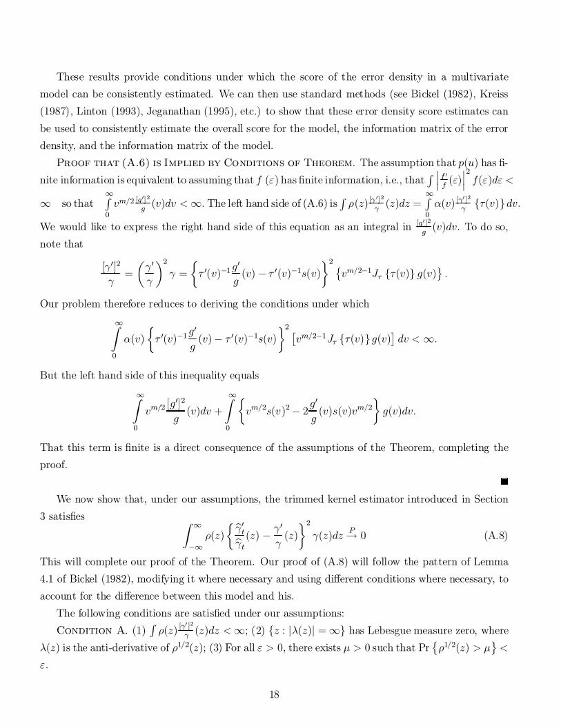
These results provide conditions under which the score of the error density in a multivariatemodel can be consistently estimated. We can then use standard methods (see Bickel (1982), Kreiss(1987), Linton (1993), Jeganathan (1995), etc.) to show that these error density score estimates canbe used to consistently estimate the overall score for the model, the information matrix of the errordensity, and the information matrix of the model.
Proof that (A.6) is Implied by Conditions of Theorem. The assumption that p(u) has ¯-nite information is equivalent to assuming that f (") has ¯nite information, i.e., that
R ¯¯f 0f (")
¯¯2f(")d" <
1 so that1R0vm=2 [g
0]2g (v)dv <1: The left hand side of (A.6) is
R½(z)[°
0]2° (z)dz =
1R0®(v) [°
0 ]2° f¿(v)gdv:
We would like to express the right hand side of this equation as an integral in [g0 ]2g (v)dv: To do so,
note that
[°0]2
°=
µ°0
°
¶2
° =½¿ 0(v)¡1g
0
g(v) ¡ ¿ 0(v)¡1s(v)
¾2 ©vm=2¡1J¿ f¿(v)g g(v)
ª:
Our problem therefore reduces to deriving the conditions under which
1Z
0
®(v)½¿ 0(v)¡1
g0
g(v)¡ ¿ 0(v)¡1s(v)
¾2 £vm=2¡1J¿ f¿(v)gg(v)
¤dv < 1:
But the left hand side of this inequality equals
1Z
0
vm=2[g0]2
g(v)dv +
1Z
0
½vm=2s(v)2 ¡ 2
g0
g(v)s(v)vm=2
¾g(v)dv:
That this term is ¯nite is a direct consequence of the assumptions of the Theorem, completing theproof.
We now show that, under our assumptions, the trimmed kernel estimator introduced in Section3 satis¯es Z 1
¡1½(z)
½b°0tb°t(z) ¡ °
0
°(z)
¾2
°(z)dz P! 0 (A.8)
This will complete our proof of the Theorem. Our proof of (A.8) will follow the pattern of Lemma4.1 of Bickel (1982), modifying it where necessary and using di®erent conditions where necessary, toaccount for the di®erence between this model and his.
The following conditions are satis¯ed under our assumptions:Condition A. (1)
R½(z) [°
0 ]2° (z)dz <1; (2) fz : j¸(z)j = 1g has Lebesgue measure zero, where
¸(z) is the anti-derivative of ½1=2(z); (3) For all " > 0, there exists ¹ > 0 such that Pr©½1=2(z) > ¹
ª<
":
18
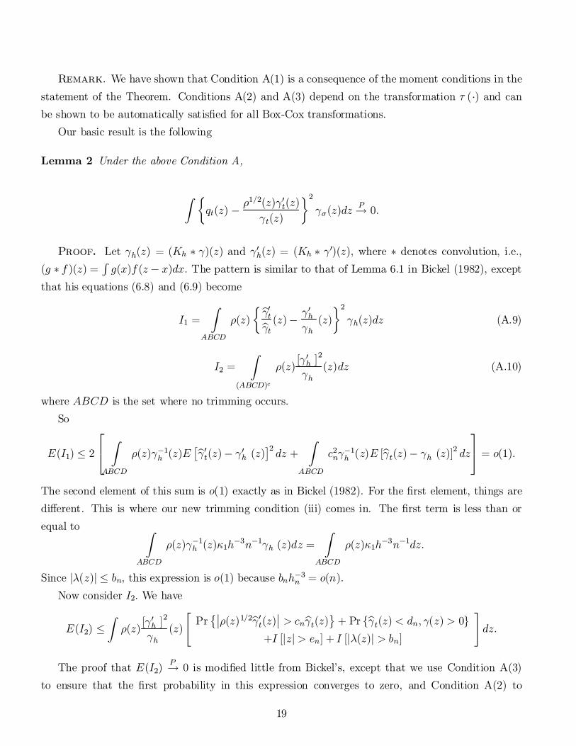
Remark. We have shown that Condition A(1) is a consequence of the moment conditions in thestatement of the Theorem. Conditions A(2) and A(3) depend on the transformation ¿ (¢) and canbe shown to be automatically satis¯ed for all Box-Cox transformations.
Our basic result is the following
Lemma 2 Under the above Condition A,
Z ½qt(z) ¡ ½
1=2(z)°0t(z)°t(z)
¾2
°¾(z)dzP! 0:
Proof. Let °h(z) = (Kh ¤ °)(z) and °0h(z) = (Kh ¤ °0)(z); where ¤ denotes convolution, i.e.,(g ¤ f )(z) =
Rg(x)f (z ¡ x)dx: The pattern is similar to that of Lemma 6.1 in Bickel (1982), except
that his equations (6.8) and (6.9) become
I1 =Z
ABCD
½(z)½b°0t
b°t(z)¡ °
0h
°h(z)
¾2
°h(z)dz (A.9)
I2 =Z
(ABCD)c
½(z) [°0h ]
2
°h(z)dz (A.10)
where ABCD is the set where no trimming occurs.So
E(I1) · 2
24
Z
ABCD
½(z)°¡1h (z)E£b°0t(z)¡ °0h (z)
¤2 dz +Z
ABCD
c2n°¡1h (z)E [b°t(z)¡ °h (z)]2 dz
35 = o(1):
The second element of this sum is o(1) exactly as in Bickel (1982). For the ¯rst element, things aredi®erent. This is where our new trimming condition (iii) comes in. The ¯rst term is less than orequal to Z
ABCD
½(z)°¡1h (z)·1h¡3n¡1°h (z)dz =Z
ABCD
½(z)·1h¡3n¡1dz:
Since j¸(z)j · bn; this expression is o(1) because bnh¡3n = o(n):Now consider I2: We have
E(I2) ·Z½(z) [°
0h ]
2
°h(z)
"Pr
©¯½(z)1=2b°0t(z)
¯> cnb°t(z)
ª+ Pr fb°t(z) < dn; °(z) > 0g
+I [jzj> en] + I [j¸(z)j > bn]
#dz:
The proof that E(I2)P! 0 is modi¯ed little from Bickel's, except that we use Condition A(3)
to ensure that the ¯rst probability in this expression converges to zero, and Condition A(2) to
19
ensure that the second indicator function is equal to zero in the limit almost everywhere. One other
modi¯cation is that we must show thatR½(z) [°
0h ]
2
°h(z)dz < 1: We can show that this holds for the
class of transformations ¿ described in the main text due to our assumption thatR ½(z)°0(z)2
°(z) dz <1:
Lemmas 6.2 and 6.3 of Bickel (1982) can be applied to our model to complete the proof of theTheorem.
References
[1] Banz, R. 1981. The relation between return and market value of common stocks. Journal ofFinancial Economics 9:3-18.
[2] Basu, S. 1977. The investment performance of common stocks in relation the their price toearnings ratios: a test of the e±cient market hypothesis. Journal of Finance 32:663-682.
[3] Beran, R. 1979. Testing for ellipsoidal symmetry of a multivariate density. Annals of Statistics7:150-162.
[4] Berk, J. 1997. Necessary conditions for the CAPM. Journal of Economic Theory 73:245-257.
[5] Bickel, P.J. 1982. On adaptive estimation. Annals of Statistics 10:647-671.
[6] Black, F., M. Jensen, and M. Scholes. 1972. The capital asset pricing model: someempirical tests. In Jensen, M. (ed), Studies in the theory of Capital Markets, New York, Praeger.
[7] Bollerslev, T. 1987. A conditional heteroskedastic time series model for speculative prices
and rates of returns. Review of Economic and Statistics, 69: 542-547.
[8] Bollerslev, T., R. Engle, and J. Wooldridge. 1988. A capital asset pricing model withtime varying covariances. Journal of Political Economy 96: 116-131.
[9] Box, G. and D. Cox. 1964. An analysis of transformations. Journal of the Royal StatisticalSociety, Series B, 211-264.
[10] Campbell, J., W. Lo, and A. C. MacKinlay. 1997. The Econometrics of Financial Mar-kets. Princeton: Princeton University Press.
[11] Casella, G. and R.L. Berger. 1990. Statistical Inference. Belmont, CA: Duxbury Press.
20
[12] Chamberlain, G. 1983. A characterization of the distributions that imply mean-varianceutility functions. Journal of Economic Theory 29:185-201.
[13] Davidson, R. and J., MacKinnon. 1998. Graphical methods for investigating the size andpower of hypothesis tests. The Manchester School 66, 1-26.
[14] Fama, E. 1963. Mandelbrot and the stable Paretian hypothesis. Journal of Business 36: 420-429.
[15] Fama, E. 1965. The behaviour of stock market prices. Journal of Business 38:34-105.
[16] Fama, E., and K. French. 1992. The cross-section of expected returns. Journal of Finance47:427-465.
[17] Fama, E., and K. French. 1993. Common risk factors in the returns on stocks and bonds.Journal of Financial Economics 33:3-56.
[18] Fama, E., and J. MacBeth. 1973. Risk, return, and equilibrium: empirical tests. Journalof Political Economy 71:607-636.
[19] Fern¶andez, C., J. Osiewalski, and M.F.J. Steel. 1995. Modelling and inference withv-spherical distributions. Journal of the American Statistical Association 90:1331-1340.
[20] Gibbons, M.R. 1982. Multivariate tests of ¯nancial models: A new approach. Journal of Fi-nancial Economics. 10:3-27.
[21] Gibbons, M., S. Ross, and J. Shanken. 1989. A test of the e±ciency of a given portfolio.
Econometrica 57:1121-1152.
[22] HÄardle, W., and O.B. Linton. 1994. Applied nonparametric methods. In D.F. McFaddenand R.F. Engle III (eds.), The Handbook of Econometrics, Vol. IV, pp. 2295-2339, North Holland.
[23] Hodgson, D.J. 1998a. Adaptive estimation of cointegrating regressions with ARMA errors.Journal of Econometrics 85:231-268.
[24] Hodgson, D.J. 1998b. Adaptive estimation of error correction models. Econometric Theory14:44-69.
[25] Hodgson, D.J. 2000. Partial maximum likelihood and adaptive estimation in the presence ofconditional heterogeneity of unknown form. Econometric Reviews 19:175-206.
21
[26] Hodgson, D.J. and K. Vorkink. 2001. E±cient estimation of conditional asset pricingmodels. University of Rochester.
[27] Horowitz, J. 2000. Estimation of a generalized additive model with unknown link function.Forthcoming, Econometrica.
[28] Hsieh, D.A. and C.F. Manski. 1987. Monte Carlo evidence on adaptive maximum likelihoodestimation of a regression. Annals of Statistics 15:541-551.
[29] Ingersoll, J. 1987. Theory of Financial Decision Making. Totowa, NJ: Rowan & Little¯eld.
[30] Jarque, C.M. and A.K. Bera. 1980. E±cient tests for normality, heteroskedasticity, andserial independence of regression residuals. Economics Letters 6: 255-259.
[31] Jeganathan, P. 1995. Some aspects of asymptotic theory with applications to time seriesmodels. Econometric Theory 11:818-887.
[32] Kelker, D. 1970. Distribution theory of spherical distributions and a location-scale general-ization. Sankhya A 32:419-430.
[33] Kreiss, J.-P. 1987. On adaptive estimation in stationary ARMA processes. Annals of Statistics15:112-133.
[34] Lintner, J. 1965. The valuation of risky assets and the selection of risky investments in stockportfolios and capital budgets. Review of Economics and Statistics 47: 13-37.
[35] Linton, O. 1993. Adaptive estimation in ARCH models. Econometric Theory 9:539-569.
[36] Linton, O. 1995. Second order approximations in a partially linear regression model. Econo-metrica 63:1079-1113.
[37] MacKinlay, A. C. 1987. On multivariate tests of the CAPM. Journal of Financial Economics18:342-372.
[38] Mandelbrot, B. 1963. The variation of certain speculative prices. Journal of Business 36:394-419.
[39] Mardia, K.V. 1970. Measures of multivariate skewness and kurtosis with applications.Biometrika 57:519-530.
[40] Markowitz, H. 1952. Portfolio selection. Journal of Finance 12:77-91.
22
[41] Markowitz, H. 1959. Portfolio Selection: E±cient Diversi¯cation of Investment. New York:Wiley.
[42] Mitchell, A.F.S. 1989. The information matrix, skewness tensor and ®-connections for thegeneral multivariate elliptic distribution. Annals of the Institute of Mathematical Statistics(Tokyo) 41:289-304.
[43] Mossin, J. 1966. Equilibrium in a capital asset market. Econometrica 34:768-783.
[44] Muirhead, R.J. 1982. Aspects of Multivariate Statistical Theory. New York: Wiley.
[45] Nelson, D. 1991. Conditional heteroskedasticity in asset returns: A new approach, Econo-metrica. 59: 347-370.
[46] Owen, J., and R. Rabinovitch. 1983. On the class of elliptical distributions and theirapplications to the theory of portfolio choice. Journal of Finance 38:745-752.
[47] Phillips, P.C.B., J.W. McFarland, and P.C. McMahon. 1996. Robust tests of for-ward exchange market e±ciency with empirical evidence from the 1920's. Journal of AppliedEconometrics 11:1-22.
[48] Schick, A. 1987. A note on the construction of asymptotically linear estimators. Journal ofStatistical Planning and Inference 16:89-105.
[49] Schuster, E.F. 1985. Incorporating support constraints into nonparametric estimators of den-sities. Communications in Statistics - Theory and Methods 14:1123-1136.
[50] Sharpe, W. 1964. Capital asset prices: A theory of market equilibrium under conditions ofrisk. Journal of Finance 19:425-442.
[51] Silverman, B.W. 1986. Density Estimation for Statistics and Data Analysis. London: Chap-man & Hall.
[52] Stambaugh, R.F. 1982. On the exclusion of assets from tests of the two-parameter model: Asensitivity analysis. Journal of Financial Economics 10:237-268.
[53] Stone, C. 1975. Adaptive maximum likelihood estimation of a location parameter. Annals ofStatistics 3:267-284.
[54] Stute, W. and Werner, U. 1991. Nonparametric estimation of elliptically contoured den-sities. In Roussas, G. (ed.), Nonparametric Functional Estimation and Related Topics, KluwerAcademic Publishers, pp. 173-190.
23
[55] Tobin, J. 1958. Liquidity preference as behavior towards risk. Review of Economic Studies25:65-86.
[56] Van Praag B. and A. Wesselman, 1987. Elliptical regression operationalized. EconomicsLetters 23:269-274.
[57] White, H. 1980. A heteroskedasticity-consistent covariance matrix estimator and a direct testfor heteroskedasticity. Econometrica 48:817-838.
[58] Zhou, G. (1993). Asset pricing tests under alternative distributions. Journal of Finance,48:1927-1942.
24
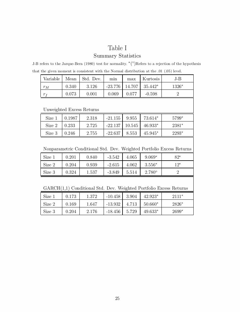
Table ISummary Statistics
J-B refers to the Jarque-Bera (1980) test for normality. ¤(¦)Refers to a rejection of the hypothesis
that the given moment is consistent with the Normal distribution at the .01 (.05) level.
Variable Mean Std. Dev. min max Kurtosis J-B
rM 0.340 3.126 -23.776 14.707 35.442¤ 1326¤
rf 0.073 0.001 0.069 0.077 -0.598 2
Unweighted Excess Returns
Size 1 0.1987 2.318 -21.155 9.955 73.614¤ 5799¤
Size 2 0.233 2.725 -22.137 10.545 46.933¤ 2381¤
Size 3 0.246 2.755 -22.637 8.553 45.945¤ 2293¤
Nonparametric Conditional Std. Dev. Weighted Portfolio Excess Returns
Size 1 0.201 0.840 -3.542 4.065 9.069¤ 82¤
Size 2 0.204 0.939 -2.615 4.062 3.556¤ 12¤
Size 3 0.324 1.537 -3.849 5.514 2.780¦ 2
GARCH(1,1) Conditional Std. Dev. Weighted Portfolio Excess Returns
Size 1 0.173 1.372 -10.458 3.904 42.923¤ 2111¤
Size 2 0.169 1.647 -13.932 4.713 50.660¤ 2826¤
Size 3 0.204 2.176 -18.456 5.729 49.633¤ 2699¤
25
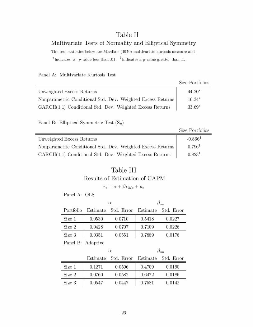
Table IIMultivariate Tests of Normality and Elliptical SymmetryThe test statistics below are Mardia's (1970) multivariate kurtosis measure and¤Indicates a p-value less than .01. 1Indicates a p-value greater than .1.
Panel A: Multivariate Kurtosis TestSize Portfolios
Unweighted Excess Returns 44.20¤
Nonparametric Conditional Std. Dev. Weighted Excess Returns 16.34¤
GARCH(1,1) Conditional Std. Dev. Weighted Excess Returns 33.69¤
Panel B: Elliptical Symmetric Test (Sn)Size Portfolios
Unweighted Excess Returns -0.8661
Nonparametric Conditional Std. Dev. Weighted Excess Returns 0.7961
GARCH(1,1) Conditional Std. Dev. Weighted Excess Returns 0.8231
Table IIIResults of Estimation of CAPM
rt = ®+ ¯rM;t + utPanel A: OLS
® ¯imPortfolio Estimate Std. Error Estimate Std. Error
Size 1 0.0530 0.0710 0.5418 0.0227
Size 2 0.0428 0.0707 0.7109 0.0226
Size 3 0.0351 0.0551 0.7889 0.0176Panel B: Adaptive
® ¯imEstimate Std. Error Estimate Std. Error
Size 1 0.1271 0.0596 0.4709 0.0190Size 2 0.0760 0.0582 0.6472 0.0186
Size 3 0.0547 0.0447 0.7581 0.0142
26
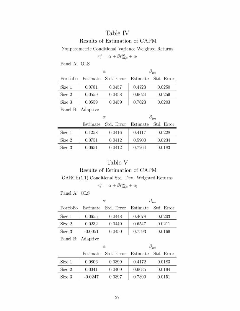
Table IVResults of Estimation of CAPM
Nonparametric Conditional Variance Weighted Returnsrwt = ® + ¯rwM;t + ut
Panel A: OLS® ¯im
Portfolio Estimate Std. Error Estimate Std. Error
Size 1 0.0781 0.0457 0.4723 0.0250Size 2 0.0559 0.0458 0.6624 0.0259
Size 3 0.0559 0.0459 0.7623 0.0203Panel B: Adaptive
® ¯imEstimate Std. Error Estimate Std. Error
Size 1 0.1258 0.0416 0.4117 0.0228
Size 2 0.0751 0.0412 0.5900 0.0234Size 3 0.0651 0.0412 0.7264 0.0183
Table VResults of Estimation of CAPM
GARCH(1,1) Conditional Std. Dev. Weighted Returnsrwt = ® + ¯rwM;t + ut
Panel A: OLS® ¯im
Portfolio Estimate Std. Error Estimate Std. Error
Size 1 0.0655 0.0448 0.4678 0.0203Size 2 0.0232 0.0449 0.6547 0.0211
Size 3 -0.0051 0.0450 0.7593 0.0169Panel B: Adaptive
® ¯imEstimate Std. Error Estimate Std. Error
Size 1 0.0806 0.0399 0.4172 0.0183
Size 2 0.0041 0.0409 0.6035 0.0194Size 3 -0.0247 0.0397 0.7390 0.0151
27
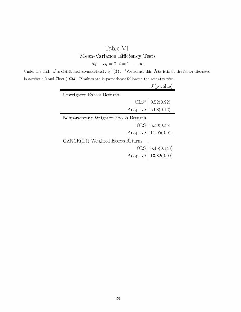
Table VIMean-Variance E±ciency Tests
H0 : ®i = 0 i = 1; : : : ;m:Under the null, J is distributed asymptotically Â2 (3) . ¤We adjust this Jstatistic by the factor discussed
in section 4.2 and Zhou (1993). P-values are in parentheses following the test statistics.
J (p-value)
Unweighted Excess ReturnsOLS¤ 0.52(0.92)
Adaptive 5.68(0.12)
Nonparametric Weighted Excess ReturnsOLS 3.30(0.35)
Adaptive 11.05(0.01)
GARCH(1,1) Weighted Excess ReturnsOLS 5.45(0.148)
Adaptive 13.82(0.00)
28

Figure Information
Figure 1. P-value Plot for ut s t(3)Figure 2. Power-Size Plot for ut s t(3)Figure 3. P-value Plot for ut s MN1
Figure 4. Power-Size Plot for ut sMN1
Figure 5. P-value Plot for ut s MN2
Figure 6. Power-Size Plot for ut sMN2
Figure 7. Power-Size Plot for both ut s MN1 and MN2
29