- 1 -

Testing Happiness Hypothesis among the Elderly

Alejandro Cid (∗ ) Daniel Ferrés (∗ ) Máximo Rossi (∗ ∗ )

September 2007

Abstract

A growing strand of economic literature focuses its attention on the relationship between

happiness levels and various individual and socioeconomic variables. Recent studies analyze

the impact of income, marital status, health, educational levels and other socioeconomic

variables on satisfaction with life. A large majority of these studies limit their attention to

industrialized countries. In our work, we analyze data for a group of individuals living in a Latin

American country (Uruguay) with age 60 or older. We use a rich data set that allows us to test

different happiness hypothesis employing four methodological approaches. We find that older

people in Uruguay have a tendency to report themselves happy when they are married, when

they have higher standards of health and when they earn higher levels of income or they feel

their income is suitable for their standard of living. On the contrary, they report lower levels of

happiness when they live alone and when their nutrition is insufficient. We also find that

education has no clear impact on happiness. We think that our study is an initial contribution to

the study of those factors that can explain happiness among the elderly in Latin American

countries. Future work will focus on enhanced empirical analysis and in extending our study to

other countries.

Keywords: Happiness, Health, Family, Censored Econometric Models, Semiparametric Methods, Treatment Evaluation JEL codes: C14, C24, I10, J12

∗ Departamento de Economía, Universidad de Montevideo (acid@um.edu.uy and dferres@um.edu.uy) ∗ ∗ Departamento de Economía, FCS, Universidad de la República (mito@decon.edu.uy)

- 2 -

1. Introduction

Fresh interest among economists in using surveys of reported well being as a way to measure

individual utility and its relation to a range of economic and social phenomena provides a new tool

to understand what causes happiness.

A large body of research on happiness in economics takes reported subjective well-being as a

proxy measure for utility. In particular, “happiness” is defined as satisfaction with life in general.1

Based on the analysis of survey data on subjective well-being, current work is guided by the

question: “how does x affect happiness?”, where x can be income, health, marital status or

employment status.

Different relationships between happiness and specific variables have been explored in recent

economic work. In particular, various scholars have devoted good amount of effort trying to assess

the relationship between income and happiness. This issue is particularly attractive to many people

for one reason: there is vast evidence indicating that differences in income explain only a low

proportion of the differences in happiness among persons. Also, although many countries have

experienced strong rises in their per capita GDP, it is not generally true that these countries have

seen average happiness to rise. This observation is particularly true for the cases of the US, the

UK, Japan and Belgium. Scholars, puzzled by this surprising observation, have worked in order to

come up with new hypothesis trying to explain subjective well-being. In particular, recent work has

focused in testing the relevance of inequality, relative income and income aspirations when trying to

understand what causes happiness.

Alesina et al (2003) studied the effect of income inequality in society on individual well-being. In

their work, they found that “individuals have a lower tendency to report themselves happy when

inequality is high, even after controlling for individual income”. They compared results obtained for

European countries and the United States.2 Interestingly, their results are clearly different across

socioeconomic groups in Europe and the US. In particular, they found that in Europe the poor and

those on the left of the political spectrum become unhappy as inequality grows. On the other hand,

in the US, the happiness of the poor and of those on the left is uncorrelated with inequality.

1 Most studies are based on surveys that contain the following question: “How satisfied are you with your life?”. 2 For the US, they present data by state.

- 3 -

Frey and Stutzer (2003) tested different happiness hypothesis. In particular, they conducted an

empirical test of the role of income aspirations. Their idea is based on the observation that many

people compare themselves to those that are considered their others. In the past, many economists

have explored this idea when trying to understand different socioeconomic phenomena. Frey and

Stutzer concluded that “the evidence presented indicates that people’s well-being is better

understood when their income aspirations are taken into consideration.”

Clark and Oswald (1994) analyzed the impact of unemployment in happiness using data from

the British Household Panel Study (1991). In their work, they constructed a “caseness score” using

12 questions present in the survey. After controlling for specific individual characteristics, they

utilized ordered probit estimation in order to explore the relationship between unemployment and

mental well-being. They concluded that there is a strong negative relationship between these

variables. Moreover, they observed that the effect of unemployment on well-being can be stronger

“than any other single characteristic, including important negative ones such as divorce and

separation”.

Other economists have examined the relationship between happiness and different individual

variables. Stack and Eshleman (1998) analyzed the relationship between marriage and happiness

in a multi-country study. In particular, they observed that the positive relationship between being

married and happiness indicators held for 16 of the 17 cases analyzed.

Health status is another factor that can be expected to be an especially important determinant of

happiness. Gerdtham and Johannesson (1997) analyzed the relationship between happiness and

health status based on data on a sample of 5,000 individuals in the Swedish adult population. In

their study, they found a positive and statistically significant relationship between higher health

status and happiness.

So far, most of the research on the relationship between individual characteristics and

happiness has focused on industrialized countries. It is evident that factors affecting satisfaction

with life may vary from region to region. The impact of income or family composition on happiness

can be very much related with cultural issues. Interestingly, Graham and Felton (2005)

analyzed the effect of income inequality on happiness in Latin America. Their work is based on data

gathered in Latinobarometro.

Our work represents a fresh attempt to understand the factors that may be related to a

higher satisfaction with life in Uruguay, a Latin American country. In particular we will explore the

correlation between happiness and income, family structure and health.

- 4 -

Correlations do not establish causation. In this sense, we understand that a crucial aspect of

our future work will be related to trying to understand the way in which causality goes. A happiness

function assumes that the right hand variables determine the level of the dependent variable. In the

case of our study, we are aware that there may also be a reverse causation. For example, are

happy people more likely to be married or is it that marriage causes happiness? In order to explore

and deal with this selection bias we employ the propensity score technique.

The rest of the paper continues as follows. In section 2 we describe the data set and different

happiness indicators. In section 3 we deal with multiple methodological aspects of our work. In

section 4 we present the obtained results. In section 5 we present the p-score results. In section 6

we conclude.

2. Data and happiness indicators

Data

Our analysis of the determinants of happiness in Uruguay relies on data from a multicountry

survey called Salud, Bienestar y Envejecimiento en América Latina y el Caribe (SABE), a study

sponsored by the Pan American Health Organization (PAHO)3. Since the survey is limited to the

single-largest city in each country, we focus on information for Montevideo (1,444 observations).

SABE data was collected in 1999-2000.

Since the survey gathers information about the elderly, the sampling frame limits its scope to

those 60 and older. Individuals living in institutions, such as nursing homes and mental institutions

are excluded from the sample. Table 1 presents descriptive statistics of both dependent and

independent variables.

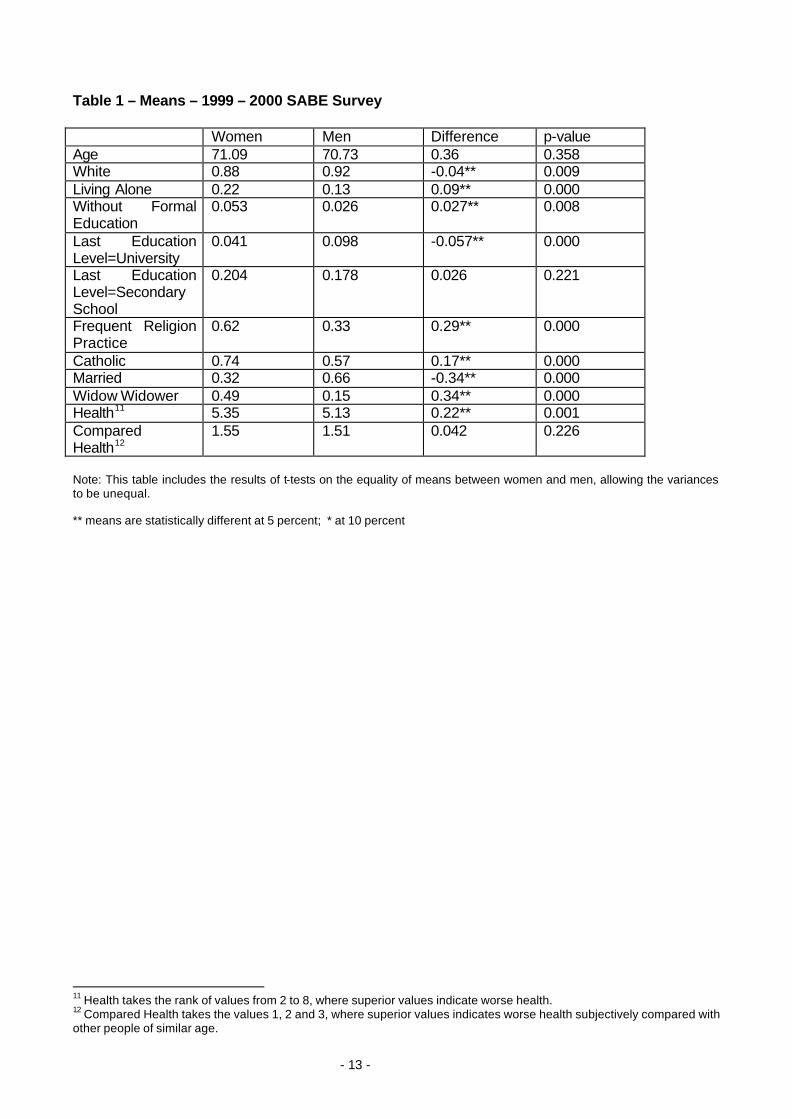
[Insert Table 1]

Independent variables include indications of age, gender, family structure, education, health status,

employment status and income. Information on these variables is present on SABE, except for

income.4 The income variable is a constructed variable, obtained after extrapolating data from

Encuesta Continua de Hogares. Our approach conducts to a fresh indication of the individual

income level (see Appendix A for details) and is different from the analysis of Graham and Felton

(2005) who constructed an “asset index” based on household possessions.

3 The survey includes information for Argentina, Barbados, Brazil, Chile, Cuba, Mexico and Uruguay. 4 Although SABE has an “Income” chapter, data on income is rather incomplete in the Uruguayan survey.

- 5 -

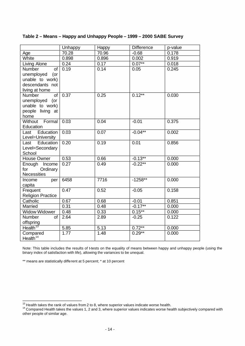
Table 2 presents mean values for the independent variable among the happy and the

unhappy. [Insert Table 2] Happiness Indicators

Our objective is to test how individual’s judgment of well-being is affected by a group of

individual characteristics and socioeconomic variables. We follow two paths when defining the

dependent variable. Constructing two types of “happiness” indicators will allow us to conduct more

robust econometric analysis about the impact of specific variables on happiness. We believe that

this issue constitutes a strong aspect of our estimation approach.

First, we construct a dummy variable indicating “satisfaction with life”. This variable is

constructed based on the following question: “In the last two weeks: have you been satisfied with

your life?” Respondents can answer “yes” o “no”. We use this binary variable in a probit estimation.

Also we built an index of happiness based on 15 binary responses to questions related with life

satisfaction (for each question, a 0 is assigned to “No” and 1 to “Yes”). Thus, this index takes the

integer values from 0 to 15, where superior values mean greater life satisfaction. We used this

definition of happiness when conducting OLS analysis. Finally, we expressed this index in

percentage terms in order to use it in the semiparametric model.

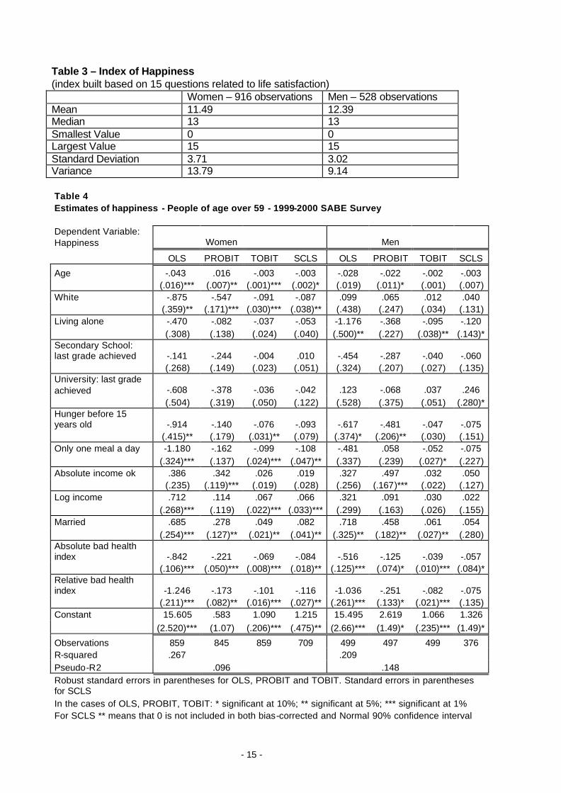
Table 3 presents descriptive statistics about the constructed happiness indicators.

[Insert Table 3]

Income and Happiness

As said, the relationship between income and happiness can be analyzed from several

different points of views. Economists have focused on issues such as the relationship between (a)

absolute income and happiness; (b) relative income and happiness; (c) income inequality and

happiness; (d) income aspirations and happiness.5 There is sufficient evidence that absolute

income, alone, does not play a substantial role explaining happiness levels. In our work we will

consider income as an independent variable but also, relative income and income aspirations.

5 Income aspirations reflect people’s perception about them having enough money for paying their daily expenses. Clearly, there is an objective, but also a subjective component in this perception.

- 6 -

Broadly speaking, relative income is defined as the difference between individual income

and the average income for the reference group. In our work we take the following approach: we

include a variable indicating the income percentile to which the respondent belongs.6 Income

aspirations information is collected from the following question: “Do you think that you (and your

partner) have enough money in order to cover your daily expenses?”

Family and Happiness

In a context of rapid transformation in typical family structures we intent to understand the

effects of changes in family composition on happiness. In this sense, since our data set focuses on

the elderly, it provides a unique opportunity to assess long term impact of divorce and remarriage

on individual happiness.

There is vast evidence about the negative impact of divorce on life satisfaction. Again, most

of this evidence is reflected by data related to industrialized countries. Our dataset allows us to

investigate the impact of marriage and divorce in the Latin American region. We know that our

dataset restricts our attention to those that were 60 or older in 1999-2000. In issues related to moral

related values, it is definitely interesting to compare our results to other studies that may contain

information for younger cohorts.

Health status and Happiness

In our work we analyze the impact of health in both absolute and relative terms. In particular we

constructed two different variables: one that indicates the self reported health condition and another

one that expresses respondents’ opinion about individual health compared to other people in their

age group. The intuition for taking both variables into account is that working with both absolute and

relative terms will enhance our understanding of happiness levels.

3. Estimation

We follow four different strategies because we understand that by proceeding in this way we

add robustness to our analysis. We believe that each of the techniques that we use presents a

potential advantage:

6 We do this to avoid difficulties to define “reference groups”.

- 7 -

Ordinary Least Square Estimation7

We run an OLS regression where a “happiness index” is the dependent variable. This

particular model estimation presents a major advantage: it is very intuitive and it has a straight

forward interpretation. On the downside, we are aware that the index is built based on answers to

15 questions (point values range from 0 to 15, where superior values indicate greater life

satisfaction). Defined in this way, “Happiness” could be seen as a doubly censored variable which

takes on the value zero and fifteen with positive probability. In other words, the dependent variable

suffers from interval censoring and OLS could provide inconsistent estimators. Another

shortcomings of the linear probability model are: a) predicted values for “Happiness” could be

negative or greater than fifteen; b) the variance of “Happiness” is probably heteroskedastic; c)

E(Happiness|x) is nonlinear.

Probit

In our study, we define a dummy variable that takes the value of 1 when individuals express

satisfaction with life. Both logit and probit models are suitable to analyze the link between

independent variables and the “satisfaction with life” variable. Probit may be more appropriate

choice for the case in which normal distribution of the dependent variable can be assumed.

Tobit

Due to the dependent variable suffers from interval censoring, we also applied a Tobit

Model. We take into account that heteroskedasticity and nonnormality result in the Tobit estimator

being inconsistent.

A Semiparametric Censored Regression Model

As said, Tobit models require some specifications of the error distribution: normality and

homoskedasticity. In order to relax these requirements, the semiparametric approach has been

proposed in the recent economic literature to provide consistent estimates for censored data. Thus

one of the advantages of the semiparametric models for censored models is that estimators are

consistent under weaker distributional assumptions. The attribute "semiparametric" in this model

comes from the fact that the distribution of the errors given the explanatory variables does not have

a known parametric form. In this work we present results for the symmetrically censored least

squares (SCLS) estimator.

7 In the empirical application of this paper, we use robust standard errors in OLS, Probit, and Tobit models to cope with the possible existence of heteroskedasticity.

- 8 -

The symmetrically censored least squares (SCLS) approach was proposed by Powell

(1986). This estimator is based on the assumption that errors are symmetrically (and

independently) distributed around zero, so is less restrictive than Tobit requirements (normally

distributed and homoskedastic errors). The SCLS estimators are consistent and asymptotically

normal for a wide class of symmetric error distributions with heteroskedasticity of unknown form (for

a summary, see Chay and Powell, 2001, or Cameron and Trivedi, 2005).

Powell (1986) states that if the underlying error terms were symmetrically distributed about zero,

and if the latent dependent variables were observable, classical least squares estimation would

yield consistent estimates. But due to the censoring, the observed dependent variable y has an

asymmetric distribution. Powell's approach consists in symmetrically censoring the dependent

variable y (it is usually known as a "symmetric trimmed" method) so that symmetry can be restored,

and then the regression coefficients can be estimated by least squares. Symmetric censoring of the

dependent variable implies that observations with values above the censoring point are dropped,

and this means that there could be a loss of efficiency due to the information dropped in those

observations. However this problem is reduced in the present paper because a relative large

sample is used.

4. Results

Table 4 presents results for the four model estimations. We present results for men and women

separately.

[Insert Table 4]

Obtained results indicate that:

• Being married has a statistically significant positive effect on happiness among men and

women8. This result is consistent Stack and Eshleman (1998). In their study, they found that

in “16 out of 17 analyses of the individual nations, marital status was significantly related to

happiness. Further, the strength of the association between being married and being happy

is remarkably consistent across nations”.

• Living alone is associated to men showing lower levels of happiness. This relationship does

not hold for women.

8 We only capture the effect of current marital status. Thus, our interpretation is referred to whether the individual is married today or not.

- 9 -

• Absolute and relative income levels are more heavily related to higher satisfaction with life

among female than among male. In fact, we barely found any statistically significant

relationship between income levels and happiness among men.

• Having bad health has a statistically significant negative effect on happiness among men

and women. The relationship holds when individuals answer about their own health status

and when they compare themselves to their “reference group”. This result is robust to the

four specifications. In this sense, it is possible to conclude that bad health is clearly related

to low levels of satisfaction with life.

• Malnutrition (“Only one meal a day”) is negatively related to happiness indicators in the case

of women. The relationship is weaker for the case of men. Additionally, results indicate that

malnutrition in the early stages of life may have long term negative effects over happiness

indicators.

• The relationship between education variables and happiness is ambiguous. Nothing can be

concluded about the impact of higher education over happiness levels. Care is required

when interpreting this result since our sample restricts attention to those 60 or older. The

obtained result might imply that education level is not relevant when explaining happiness

levels of the elderly. Our results are in the line of those obtained by Graham et al.

• Most works that intend to explain happiness focus on the relationship between being

unemployed and satisfaction with life. In our case, we believe that due to the fact that our

data set restricts attention to those 60 or older, it is wise not to try to explore this

relationship.

In sum, we find that our results are pretty much in line with those obtained by other studies but

in this case for a not industrialized country. Individuals that have higher health levels, are or feel

richer and are married show higher levels of satisfaction with life. We also find some evidence

showing that malnutrition and living alone is negatively related to happiness.

5. Treatment Evaluation and Marital Status

The typical dilemma in treatment evaluation involves the inference of a causal association

between the treatment and the outcome. In this paper, we pay particular attention to the effects of

personal marital status on their happiness. Thus, we observe (yi,xi,Di), i=1,...,N, where yi is the

- 10 -

happiness index, xi represents the regressors, and Di is the treatment variable and takes the value

1 if the treatment is applied (got married) and is 0 otherwise. The impact of a hypothetical change in

D on y, holding x constant, is of interest. But no individual is simultaneously observed in both states.

Moreover, the sample does not come from a randomized social experiment: it comes from

observational data and the assignment of individuals to the treatment and control groups is not

random. Hence, we estimate the treatment effects based on propensity score: this approach is a

way to reduce the bias performing comparisons of outcomes using treated and control individuals

who are as similar as possible (Becker and Ichino 2002). The propensity score is defined as the

conditional probability of receiving a treatment given pre-treatment characteristics:

p(X)=Pr{D=1|X}=E{D|X}

where D={0,1} is the indicator of exposure to treatment and X is the vector of pre-treatment

characteristics.

The propensity score was estimated in this application using a Probit model9. Due to the

probability of observing two units with exactly the same value of the propensity score is in principle

zero since p(X) is a continuous variable, various methods have been developed in previous

literature (for a summary, see Cameron et alt. 2005) to match comparison units sufficiently close to

the treated units. In the present paper, after estimating p(X) we employed the Kernel Matching

method.10

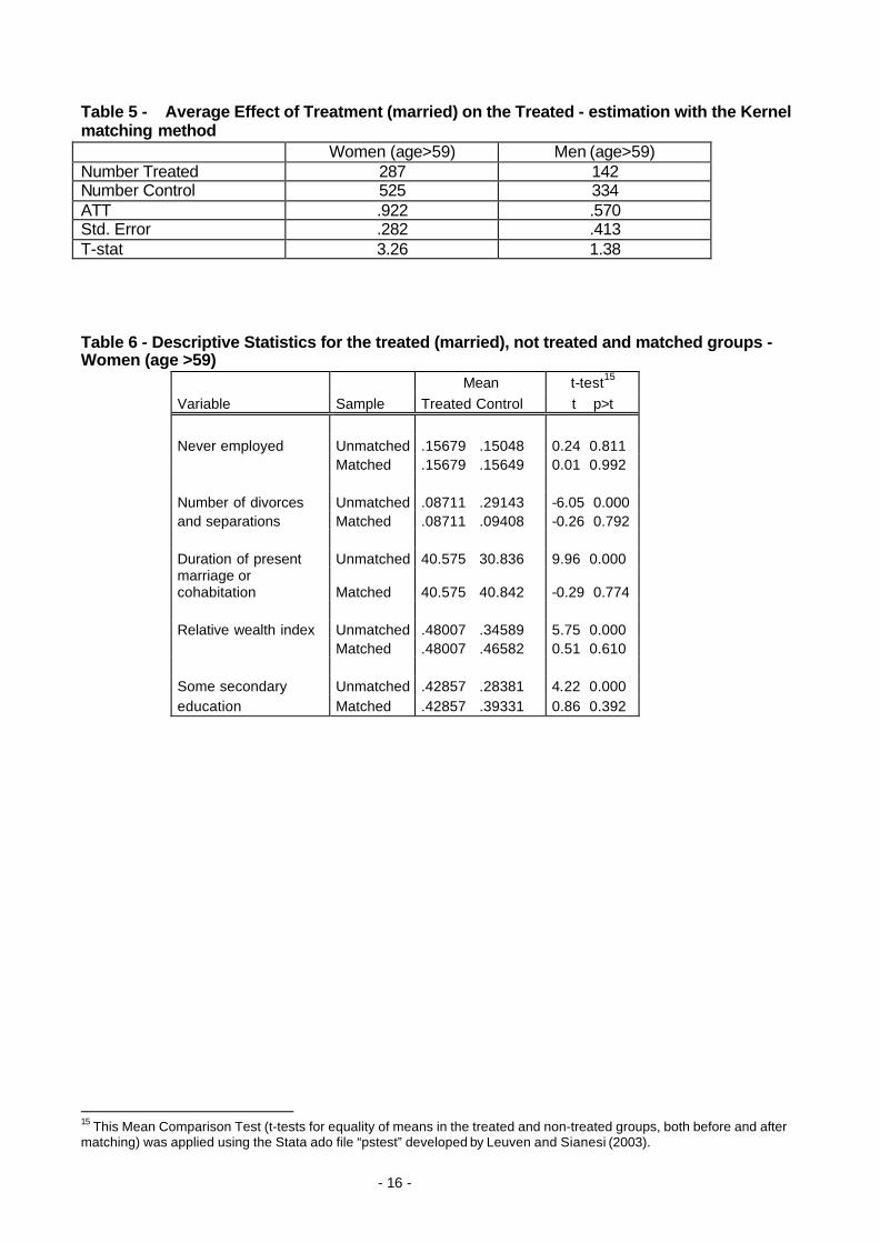
The tables below show the result:

[Insert Table 5]

In the case of men, though the “Average Effect of Treatment (got married) on the Treated” is

positive at a 90 percent, the 95 percent confidence interval includes zero. In the case of women, the

point estimates indicate that being married increases happiness and it is significantly different from

zero. Thus, data suggest positive association between being married and happiness, especially in

the case of women with age above 59.

As we have said in the beginning of this section, the matching method intends to made

comparisons between treated and control individuals who are as similar as possible. Thus, in order

to gauge the goodness of the matching, we built the tables below. This similarity between the

treated and control individuals can be seen in the mean comparison test (t-test) shown on the table: 9 Applied with the Stata ado file “pscore” developed by Becker and Ichino (2002) 10 This matching method was applied using the Stata ado file “psmatch2” developed by Leuven and Sianesi (2003).

- 11 -

there’s no statistically significant difference in the characteristics of the treated and control matched

individuals.

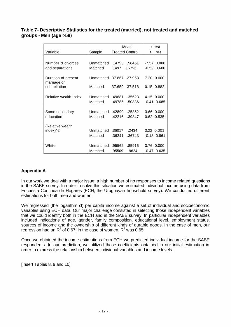
[Insert Table 6 and 7]

6. Conclusion

We perform empirical analysis in order to test various happiness theories in a group of older

people in a Latin American country. In particular, we analyzed data from Uruguay gathered by

SABE.

We find that older people in Uruguay have a tendency to report themselves happy when

they are married, when they have higher standards of health and when they earn higher levels of

income. However, the relationship between income and happiness is far stronger in the case of

women than when men are asked. When we analyze the impact of health and income on happiness

we include variables indicating absolute and relative indications. Results indicate that accounting for

relative positions improves our understanding of those factors affecting happiness. This implies that

individuals often compare themselves with their reference groups.

Individuals report lower levels of happiness when they live alone and when their nutrition is

insufficient. In the case of nutrition, we included a variable indicating malnutrition while the

individual was a child and also a dummy variable signaling whether the person eats one meal a day

or less. We also find that education has no clear impact on happiness.

Obtained results are robust to different methodological strategies. Observed relationships

are consistent with those present in the literature analyzing the case for industrialized countries. In

this sense, our work is an initial attempt in order to explore those factors that affect individual

happiness in Latin American countries. This issue has received little attention from economists.

Our study presents various limitations: Our future efforts will focus on three aspects: 1) to

extend analyses to additional countries (Brazil, Argentina, Chile, and Mexico); 2) to incorporate

additional semiparametric analysis of the relationships and 3) to incorporate enhanced analysis of

endogeneity.

- 12 -

References Alesina, A., Di Tella, R. and MacCulloch, R. (2004). “Inequality and happiness: are Europeans and Americans different?” Journal of Public Economics. 2009-2042. Becker,S. and Ichino, A. (2002). "Estimation of average treatment effects based on propensity scores", The Stata Journal (2002) Vol.2, No.4, pp. 358-377. Clark, A. E. and Oswald, A. J. (1994). “Unhappiness and Unemployment”. The Economic Journal, Vol 104, No 424, pp. 648-659. Cameron, A. C. and Trivedi, P. K. (2005). "Microeconometrics. Methods and Applications". Cambridge University Press. Chay, K. Y. and Powell, J. L. (2001). "Semiparametric Censored Regression Models." Journal of Economic Perspectives. Fall 2001, 15:4, pp. 29-42. Frey, B. and Stutzer, A. (2002). “What can Economists learn from Happiness Research? “Journal of Economic Literature, Vol 40, No2, pp. 402-435. Frey, B. and Stutzer, A. (2003). Testing Theories of Happiness. Institute for Empirical Research in Economics, University of Zurich. Working Paper Series, No 147. Gerdtham, U and Johanesson, M. (1997). “The relationship between happiness, health and socio-economic factors: results based on Swedish micro data”. Working Paper Series in Economics and Finance No. 27. Department of Economics, Stockholm School of Economics, Stockholm, Sweden. Graham, C. and Felton, A. (2005). “Does Inequality Matter to Individual Welfare? An initial exploration based on happiness surveys from Latin America”. The Brookings Institution. Center on Social and Economic Dynamics. Working Paper No 38. Honoré, Bo E. and Powell, J. L. (1994). "Pairwise Difference Estimators for Censored and Truncated Regression Models." Journal of Econometrics. September/October, 64:1-2, pp. 241-78. Leuven, E. and Sianesi, B. (2003). "PSMATCH2: Stata module to perform full Mahalanobis and propensity score matching, common support graphing, and covariate imbalance testing". Powell, J. L. (1984). "Least Absolute Deviations Estimation for the Censored Regression Model." Journal of Econometrics. July, 25:3, pp. 303-25. Powell, J. L. (1986). "Symmetrically Trimmed Least Squares Estimation for Tobit Models." Econometrica. November, 54:6, pp. 1435-60. Stack, S. and Eshleman, J. R. (1998). “Marital Status and Happiness: A 17-Nation Study”. May, pp. 527-536. Rosenbaum, P. and Rubin, D. (1983). “The central role of the propensity score in observational studies for causal effects”. Biometrika 1983 70(1), pp. 41-55.

- 13 -

Table 1 – Means – 1999 – 2000 SABE Survey Women Men Difference p-value Age 71.09 70.73 0.36 0.358 White 0.88 0.92 -0.04** 0.009 Living Alone 0.22 0.13 0.09** 0.000 Without Formal Education

0.053 0.026 0.027** 0.008

Last Education Level=University

0.041 0.098 -0.057** 0.000

Last Education Level=Secondary School

0.204 0.178 0.026 0.221

Frequent Religion Practice

0.62 0.33 0.29** 0.000

Catholic 0.74 0.57 0.17** 0.000 Married 0.32 0.66 -0.34** 0.000 Widow Widower 0.49 0.15 0.34** 0.000 Health11 5.35 5.13 0.22** 0.001 Compared Health12

1.55 1.51 0.042 0.226

Note: This table includes the results of t-tests on the equality of means between women and men, allowing the variances to be unequal. ** means are statistically different at 5 percent; * at 10 percent

11 Health takes the rank of values from 2 to 8, where superior values indicate worse health. 12 Compared Health takes the values 1, 2 and 3, where superior values indicates worse health subjectively compared with other people of similar age.

- 14 -

Table 2 – Means – Happy and Unhappy People – 1999 – 2000 SABE Survey Unhappy Happy Difference p-value Age 70.28 70.96 -0.68 0.178 White 0.898 0.896 0.002 0.919 Living Alone 0.24 0.17 0.07** 0.018 Number of unemployed (or unable to work) descendants not living at home

0.19 0.14 0.05 0.245

Number of unemployed (or unable to work) people living at home

0.37 0.25 0.12** 0.030

Without Formal Education

0.03 0.04 -0.01 0.375

Last Education Level=University

0.03 0.07 -0.04** 0.002

Last Education Level=Secondary School

0.20 0.19 0.01 0.856

House Owner 0.53 0.66 -0.13** 0.000 Enough Income for Ordinary Necessities

0.27 0.49 -0.22** 0.000

Income per capita

6458 7716 -1258** 0.000

Frequent Religion Practice

0.47 0.52 -0.05 0.158

Catholic 0.67 0.68 -0.01 0.851 Married 0.31 0.48 -0.17** 0.000 Widow Widower 0.48 0.33 0.15** 0.000 Number of offspring

2.64 2.89 -0.25 0.122

Health13 5.85 5.13 0.72** 0.000 Compared Health14

1.77 1.48 0.29** 0.000

Note: This table includes the results of t-tests on the equality of means between happy and unhappy people (using the binary index of satisfaction with life), allowing the variances to be unequal. ** means are statistically different at 5 percent; * at 10 percent

13 Health takes the rank of values from 2 to 8, where superior values indicate worse health. 14 Compared Health takes the values 1, 2 and 3, where superior values indicates worse health subjectively compared with other people of similar age.

- 15 -

Table 3 – Index of Happiness (index built based on 15 questions related to life satisfaction) Women – 916 observations Men – 528 observations Mean 11.49 12.39 Median 13 13 Smallest Value 0 0 Largest Value 15 15 Standard Deviation 3.71 3.02 Variance 13.79 9.14 Table 4 Estimates of happiness - People of age over 59 - 1999-2000 SABE Survey Dependent Variable: Happiness Women Men

OLS PROBIT TOBIT SCLS OLS PROBIT TOBIT SCLS

Age -.043 .016 -.003 -.003 -.028 -.022 -.002 -.003 (.016)*** (.007)** (.001)*** (.002)* (.019) (.011)* (.001) (.007) White -.875 -.547 -.091 -.087 .099 .065 .012 .040 (.359)** (.171)*** (.030)*** (.038)** (.438) (.247) (.034) (.131) Living alone -.470 -.082 -.037 -.053 -1.176 -.368 -.095 -.120 (.308) (.138) (.024) (.040) (.500)** (.227) (.038)** (.143)* Secondary School: last grade achieved -.141 -.244 -.004 .010 -.454 -.287 -.040 -.060 (.268) (.149) (.023) (.051) (.324) (.207) (.027) (.135) University: last grade achieved -.608 -.378 -.036 -.042 .123 -.068 .037 .246 (.504) (.319) (.050) (.122) (.528) (.375) (.051) (.280)* Hunger before 15 years old -.914 -.140 -.076 -.093 -.617 -.481 -.047 -.075 (.415)** (.179) (.031)** (.079) (.374)* (.206)** (.030) (.151) Only one meal a day -1.180 -.162 -.099 -.108 -.481 .058 -.052 -.075 (.324)*** (.137) (.024)*** (.047)** (.337) (.239) (.027)* (.227) Absolute income ok .386 .342 .026 .019 .327 .497 .032 .050 (.235) (.119)*** (.019) (.028) (.256) (.167)*** (.022) (.127) Log income .712 .114 .067 .066 .321 .091 .030 .022 (.268)*** (.119) (.022)*** (.033)*** (.299) (.163) (.026) (.155) Married .685 .278 .049 .082 .718 .458 .061 .054 (.254)*** (.127)** (.021)** (.041)** (.325)** (.182)** (.027)** (.280) Absolute bad health index -.842 -.221 -.069 -.084 -.516 -.125 -.039 -.057 (.106)*** (.050)*** (.008)*** (.018)** (.125)*** (.074)* (.010)*** (.084)* Relative bad health index -1.246 -.173 -.101 -.116 -1.036 -.251 -.082 -.075 (.211)*** (.082)** (.016)*** (.027)** (.261)*** (.133)* (.021)*** (.135) Constant 15.605 .583 1.090 1.215 15.495 2.619 1.066 1.326 (2.520)*** (1.07) (.206)*** (.475)** (2.66)*** (1.49)* (.235)*** (1.49)*

Observations 859 845 859 709 499 497 499 376 R-squared .267 .209 Pseudo-R2 .096 .148 Robust standard errors in parentheses for OLS, PROBIT and TOBIT. Standard errors in parentheses for SCLS In the cases of OLS, PROBIT, TOBIT: * significant at 10%; ** significant at 5%; *** significant at 1% For SCLS ** means that 0 is not included in both bias-corrected and Normal 90% confidence interval

- 16 -

Table 5 - Average Effect of Treatment (married) on the Treated - estimation with the Kernel matching method Women (age>59) Men (age>59) Number Treated 287 142 Number Control 525 334 ATT .922 .570 Std. Error .282 .413 T-stat 3.26 1.38 Table 6 - Descriptive Statistics for the treated (married), not treated and matched groups - Women (age >59)

Mean t-test15 Variable Sample Treated Control t p>t

Never employed Unmatched .15679 .15048 0.24 0.811 Matched .15679 .15649 0.01 0.992 Number of divorces Unmatched .08711 .29143 -6.05 0.000 and separations Matched .08711 .09408 -0.26 0.792 Duration of present Unmatched 40.575 30.836 9.96 0.000 marriage or cohabitation Matched 40.575 40.842 -0.29 0.774 Relative wealth index Unmatched .48007 .34589 5.75 0.000 Matched .48007 .46582 0.51 0.610 Some secondary Unmatched .42857 .28381 4.22 0.000 education Matched .42857 .39331 0.86 0.392

15 This Mean Comparison Test (t-tests for equality of means in the treated and non-treated groups, both before and after matching) was applied using the Stata ado file “pstest” developed by Leuven and Sianesi (2003).

- 17 -

Table 7- Descriptive Statistics for the treated (married), not treated and matched groups - Men (age >59)

Mean t-test Variable Sample Treated Control t p>t

Number of divorces Unmatched .14793 .58451 -7.57 0.000 and separations Matched .1497 .16752 -0.52 0.600 Duration of present Unmatched 37.867 27.958 7.20 0.000 marriage or cohabitation Matched 37.659 37.516 0.15 0.882 Relative wealth index Unmatched .49681 .35623 4.15 0.000 Matched .49785 .50836 -0.41 0.685 Some secondary Unmatched .42899 .25352 3.66 0.000 education Matched .42216 .39847 0.62 0.535 (Relative wealth index)^2 Unmatched .36017 .2434 3.22 0.001 Matched .36241 .36743 -0.18 0.861 White Unmatched .95562 .85915 3.76 0.000 Matched .95509 .9624 -0.47 0.635

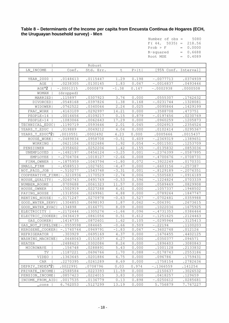
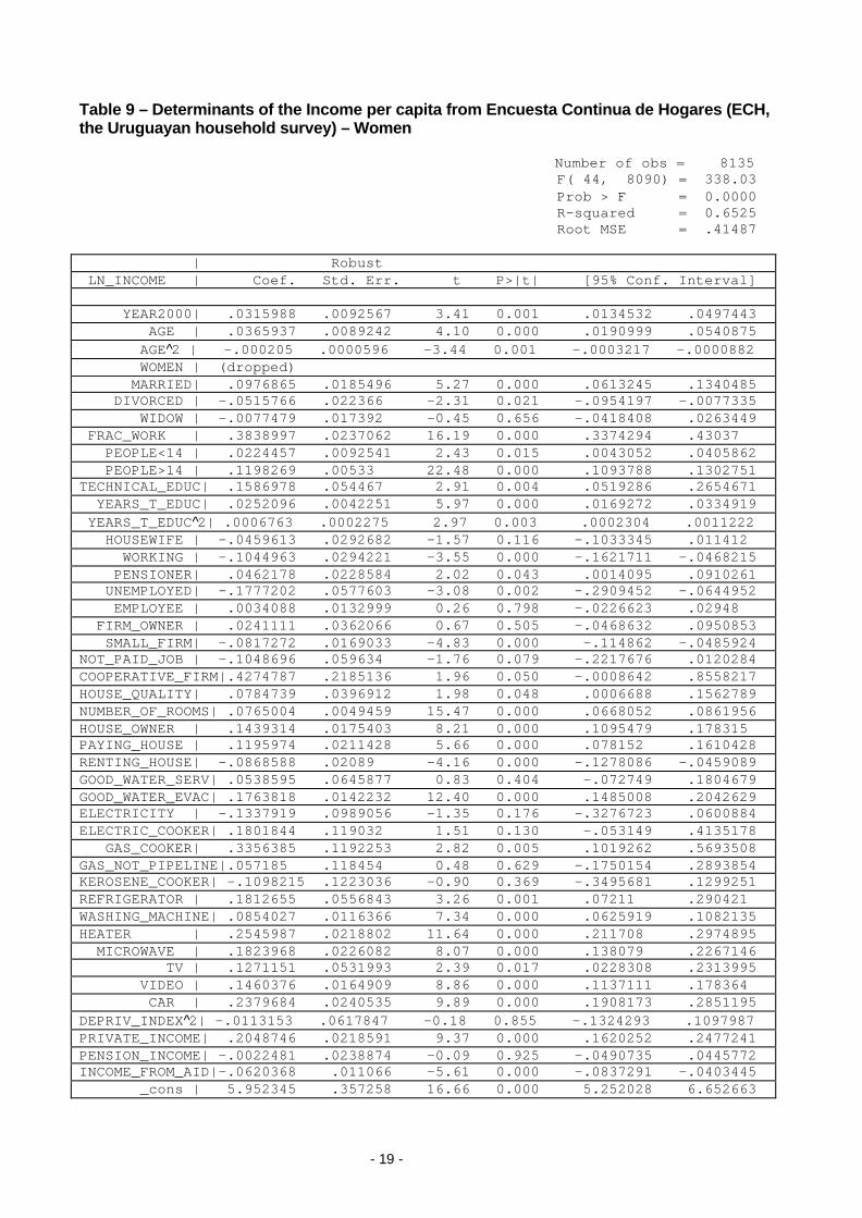
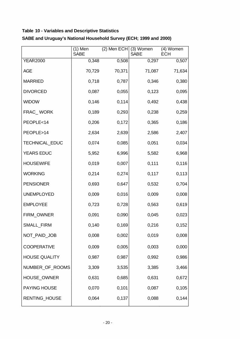
Appendix A In our work we deal with a major issue: a high number of no responses to income related questions in the SABE survey. In order to solve this situation we estimated individual income using data from Encuesta Continua de Hogares (ECH, the Uruguayan household survey). We conducted different estimations for both men and women. We regressed (the logarithm of) per capita income against a set of individual and socioeconomic variables using ECH data. Our major challenge consisted in selecting those independent variables that we could identify both in the ECH and in the SABE survey. In particular independent variables included indications of age, gender, family composition, educational level, employment status, sources of income and the ownership of different kinds of durable goods. In the case of men, our regression had an R2 of 0.67; in the case of women, R2 was 0.65. Once we obtained the income estimations from ECH we predicted individual income for the SABE respondents. In our prediction, we utilized those coefficients obtained in our initial estimation in order to express the relationship between individual variables and income levels. [Insert Tables 8, 9 and 10]

- 18 -

Table 8 – Determinants of the Income per capita from Encuesta Continua de Hogares (ECH, the Uruguayan household survey) - Men Number of obs = 5080 F( 44, 5035) = 218.56 Prob > F = 0.0000 R-squared = 0.6688 Root MSE = 0.4089 | Robust LN_INCOME | Coef. Std. Err. t P>|t| [95% Conf. Interval] YEAR_2000 | .0148613 .0115447 1.29 0.198 -.0077713 .0374939 AGE | .0238305 .0130145 1.83 0.067 -.0016837 .0493446 AGE^2 | -.0001215 .0000879 -1.38 0.167 -.0002938 .0000508 WOMAN | (dropped) MARRIED| .115897 .0307923 3.76 0.000 .0555307 .1762632 DIVORCED| .0548168 .0397826 1.38 0.168 -.0231744 .1328081 WIDOWER| .0762522 .0340066 2.24 0.025 .0095844 .1429199 FRAC_WORK | .4163109 .0292997 14.21 0.000 .3588708 .473751 PEOPLE<14 | .0016656 .0109217 0.15 0.879 -.0197456 .0230769 PEOPLE>14 | .1083066 .0062643 17.29 0.000 .0960259 .1205873 TECHNICAL_EDUC| .1190719 .0593646 2.01 0.045 .0026913 .2354524 YEARS_T_EDUC | .019889 .0049212 4.04 0.000 .0102414 .0295367 YEARS_T_EDUC^2| .0010551 .0002492 4.23 0.000 .0005666 .0015437 HOUSE_WORK| -.0489834 .0958708 -0.51 0.609 -.2369319 .1389651 WORKING | .0621104 .0322686 1.92 0.054 -.0011501 .1253709 PENSIONER | .0358602 .0252206 1.42 0.155 -.0135832 .0853036 UNEMPLOYED | -.1482197 .0456124 -3.25 0.001 -.2376399 -.0587995 EMPLOYEE | -.2704704 .1018127 -2.66 0.008 -.4700676 -.0708731 FIRM_OWNER | -.1875959 .1043794 -1.80 0.072 -.3922249 .0170331 SMALL_FIRM | -.4588513 .1027651 -4.47 0.000 -.6603156 -.257387 NOT_PAID_JOB | -.510277 .1543748 -3.31 0.001 -.8129189 -.2076351 COOPERATIVE_FIRM|-.3210936 .1170529 -2.74 0.006 -.5505683 -.0916189 HOUSE_QUALITY| -.0260743 .0491769 -0.53 0.596 -.1224824 .0703339 NUMBER_ROOMS | .0709688 .0061323 11.57 0.000 .0589469 .0829908 HOUSE_OWNER | .1502919 .0227288 6.61 0.000 .1057337 .1948502 PAYING_HOUSE | .1318506 .0269961 4.88 0.000 .0789264 .1847747 RENTING_HOUSE| -.0171247 .0270978 -0.63 0.527 -.0702481 .0359988 GOOD_WATER_SERV| .1304853 .0698193 1.87 0.062 -.006391 .2673615 GOOD_WATER_EVAC| .134898 .0166771 8.09 0.000 .1022036 .1675925 ELECTRICITY | -.2172444 .1305276 -1.66 0.096 -.4731353 .0386464 ELECTRIC_COOKER| .0436419 .0861056 0.51 0.612 -.1251625 .2124463 GAS_COOKER| .1414735 .0872601 1.62 0.105 -.0295944 .3125413 GAS_NOT_PIPELINE|-.0559598 .084665 -0.66 0.509 -.22194 .1100203 KEROSENE_COOKER| -.1740744 .0949791 -1.83 0.067 -.3602748 .012126 REFRIGERATOR | .303929 .0695169 4.37 0.000 .1676455 .4402125 WASHING_MACHINE| .0648043 .0151837 4.27 0.000 .0350377 .094571 HEATER | .2488623 .0302086 8.24 0.000 .1896403 .3080843 MICROWAVE | .156748 .0288891 5.43 0.000 .1001128 .2133832 TV | .1187221 .0696766 1.70 0.088 -.0178743 .2553186 VIDEO | .1363645 .0201886 6.75 0.000 .096786 .1759431 CAR | .2270395 .0261289 8.69 0.000 .1758154 .2782636 DEPRIV_INDEX^2| .0022991 .0708796 0.03 0.974 -.1366559 .141254 PRIVATE_INCOME| .2588584 .0223393 11.59 0.000 .2150637 .3026532 PENSION_INCOME| .0857423 .0224015 3.83 0.000 .0418257 .129659 INCOME_FROM_AID| .0017535 .0136779 0.13 0.898 -.0250612 .0285681 _cons | 6.762053 .5127299 13.19 0.000 5.756879 7.767227

- 19 -

Table 9 – Determinants of the Income per capita from Encuesta Continua de Hogares (ECH, the Uruguayan household survey) – Women Number of obs = 8135 F( 44, 8090) = 338.03 Prob > F = 0.0000 R-squared = 0.6525 Root MSE = .41487 | Robust LN_INCOME | Coef. Std. Err. t P>|t| [95% Conf. Interval] YEAR2000| .0315988 .0092567 3.41 0.001 .0134532 .0497443 AGE | .0365937 .0089242 4.10 0.000 .0190999 .0540875 AGE^2 | -.000205 .0000596 -3.44 0.001 -.0003217 -.0000882 WOMEN | (dropped) MARRIED| .0976865 .0185496 5.27 0.000 .0613245 .1340485 DIVORCED | -.0515766 .022366 -2.31 0.021 -.0954197 -.0077335 WIDOW | -.0077479 .017392 -0.45 0.656 -.0418408 .0263449 FRAC_WORK | .3838997 .0237062 16.19 0.000 .3374294 .43037 PEOPLE<14 | .0224457 .0092541 2.43 0.015 .0043052 .0405862 PEOPLE>14 | .1198269 .00533 22.48 0.000 .1093788 .1302751 TECHNICAL_EDUC| .1586978 .054467 2.91 0.004 .0519286 .2654671 YEARS_T_EDUC| .0252096 .0042251 5.97 0.000 .0169272 .0334919 YEARS_T_EDUC^2| .0006763 .0002275 2.97 0.003 .0002304 .0011222 HOUSEWIFE | -.0459613 .0292682 -1.57 0.116 -.1033345 .011412 WORKING | -.1044963 .0294221 -3.55 0.000 -.1621711 -.0468215 PENSIONER| .0462178 .0228584 2.02 0.043 .0014095 .0910261 UNEMPLOYED| -.1777202 .0577603 -3.08 0.002 -.2909452 -.0644952 EMPLOYEE | .0034088 .0132999 0.26 0.798 -.0226623 .02948 FIRM_OWNER | .0241111 .0362066 0.67 0.505 -.0468632 .0950853 SMALL_FIRM| -.0817272 .0169033 -4.83 0.000 -.114862 -.0485924 NOT_PAID_JOB | -.1048696 .059634 -1.76 0.079 -.2217676 .0120284 COOPERATIVE_FIRM|.4274787 .2185136 1.96 0.050 -.0008642 .8558217 HOUSE_QUALITY| .0784739 .0396912 1.98 0.048 .0006688 .1562789 NUMBER_OF_ROOMS| .0765004 .0049459 15.47 0.000 .0668052 .0861956 HOUSE_OWNER | .1439314 .0175403 8.21 0.000 .1095479 .178315 PAYING_HOUSE | .1195974 .0211428 5.66 0.000 .078152 .1610428 RENTING_HOUSE| -.0868588 .02089 -4.16 0.000 -.1278086 -.0459089 GOOD_WATER_SERV| .0538595 .0645877 0.83 0.404 -.072749 .1804679 GOOD_WATER_EVAC| .1763818 .0142232 12.40 0.000 .1485008 .2042629 ELECTRICITY | -.1337919 .0989056 -1.35 0.176 -.3276723 .0600884 ELECTRIC_COOKER| .1801844 .119032 1.51 0.130 -.053149 .4135178 GAS_COOKER| .3356385 .1192253 2.82 0.005 .1019262 .5693508 GAS_NOT_PIPELINE|.057185 .118454 0.48 0.629 -.1750154 .2893854 KEROSENE_COOKER| -.1098215 .1223036 -0.90 0.369 -.3495681 .1299251 REFRIGERATOR | .1812655 .0556843 3.26 0.001 .07211 .290421 WASHING_MACHINE| .0854027 .0116366 7.34 0.000 .0625919 .1082135 HEATER | .2545987 .0218802 11.64 0.000 .211708 .2974895 MICROWAVE | .1823968 .0226082 8.07 0.000 .138079 .2267146 TV | .1271151 .0531993 2.39 0.017 .0228308 .2313995 VIDEO | .1460376 .0164909 8.86 0.000 .1137111 .178364 CAR | .2379684 .0240535 9.89 0.000 .1908173 .2851195 DEPRIV_INDEX^2| -.0113153 .0617847 -0.18 0.855 -.1324293 .1097987 PRIVATE_INCOME| .2048746 .0218591 9.37 0.000 .1620252 .2477241 PENSION_INCOME| -.0022481 .0238874 -0.09 0.925 -.0490735 .0445772 INCOME_FROM_AID|-.0620368 .011066 -5.61 0.000 -.0837291 -.0403445 _cons | 5.952345 .357258 16.66 0.000 5.252028 6.652663

- 20 -

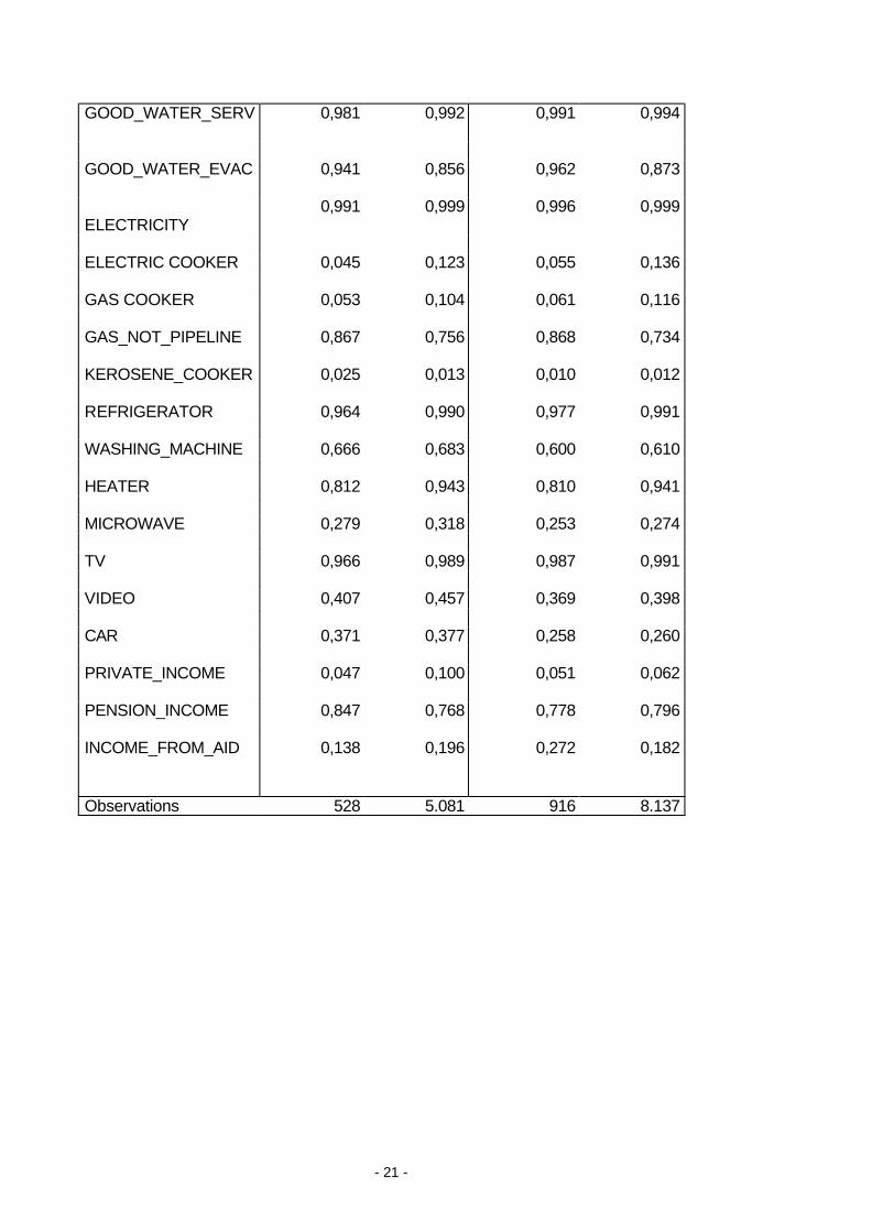
Table 10 - Variables and Descriptive Statistics

SABE and Uruguay’s National Household Survey (ECH; 1999 and 2000) (1) Men

SABE (2) Men ECH (3) Women

SABE (4) Women ECH

YEAR2000 0,348 0,508 0,297 0,507 AGE 70,729 70,371 71,087 71,634 MARRIED 0,718 0,787 0,346 0,380 DIVORCED 0,087 0,055 0,123 0,095 WIDOW 0,146 0,114 0,492 0,438 FRAC_ WORK 0,189 0,293 0,238 0,259

PEOPLE<14 0,206 0,172 0,365 0,186

PEOPLE>14 2,634 2,639 2,586 2,407

TECHNICAL_EDUC 0,074 0,085 0,051 0,034 YEARS EDUC 5,952 6,996 5,582 6,968

HOUSEWIFE 0,019 0,007 0,111 0,116 WORKING 0,214 0,274 0,117 0,113 PENSIONER 0,693 0,647 0,532 0,704 UNEMPLOYED 0,009 0,016 0,009 0,008 EMPLOYEE 0,723 0,728 0,563 0,619 FIRM_OWNER 0,091 0,090 0,045 0,023 SMALL_FIRM 0,140 0,169 0,216 0,152 NOT_PAID_JOB 0,008 0,002 0,019 0,008

COOPERATIVE 0,009 0,005 0,003 0,000

HOUSE QUALITY 0,987 0,987 0,992 0,986 NUMBER_OF_ROOMS

3,309

3,535

3,385

3,466

HOUSE_OWNER 0,631 0,685 0,631 0,672 PAYING HOUSE 0,070 0,101 0,087 0,105

RENTING_HOUSE 0,064 0,137 0,088 0,144

- 21 -

GOOD_WATER_SERV 0,981 0,992 0,991 0,994

GOOD_WATER_EVAC 0,941 0,856 0,962 0,873

ELECTRICITY

0,991 0,999 0,996 0,999

ELECTRIC COOKER 0,045 0,123 0,055 0,136 GAS COOKER 0,053 0,104 0,061 0,116 GAS_NOT_PIPELINE 0,867 0,756 0,868 0,734 KEROSENE_COOKER 0,025 0,013 0,010 0,012 REFRIGERATOR 0,964 0,990 0,977 0,991 WASHING_MACHINE 0,666 0,683 0,600 0,610 HEATER 0,812 0,943 0,810 0,941 MICROWAVE 0,279 0,318 0,253 0,274 TV 0,966 0,989 0,987 0,991 VIDEO 0,407 0,457 0,369 0,398 CAR 0,371 0,377 0,258 0,260 PRIVATE_INCOME 0,047 0,100 0,051 0,062

PENSION_INCOME 0,847 0,768 0,778 0,796

INCOME_FROM_AID 0,138 0,196 0,272 0,182

Observations 528 5.081 916 8.137