Testing Group Difference

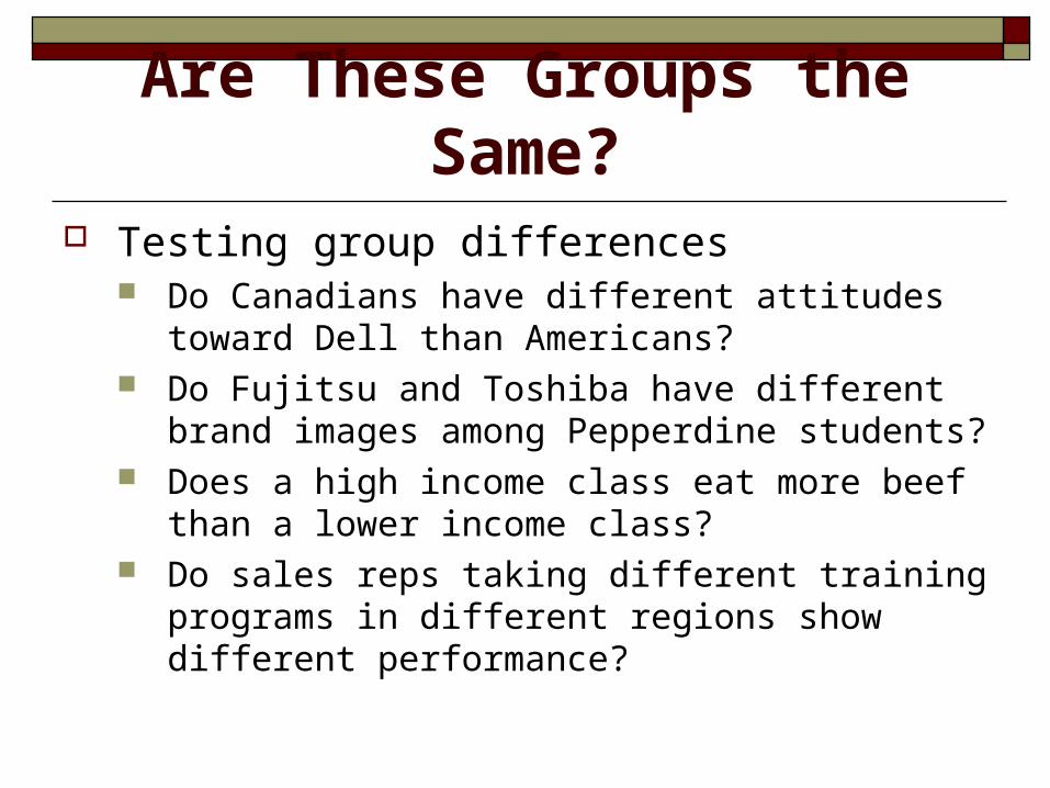
Are These Groups the Same? Testing group differences

Do Canadians have different attitudes toward Dell than Americans?

Do Fujitsu and Toshiba have different brand images among Pepperdine students?

Does a high income class eat more beef than a lower income class?

Do sales reps taking different training programs in different regions show different performance?

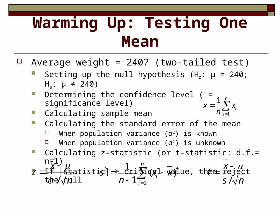
Warming Up: Testing One Mean Average weight = 240? (two-tailed test)

Setting up the null hypothesis (H0: μ = 240; Ha: μ ≠ 240) Determining the confidence level ( = significance level) Calculating sample mean Calculating the standard error of the mean

When population variance (σ2) is known When population variance (σ2) is unknown

Calculating z-statistic (or t-statistic: d.f.= n-1) If |statistic| > critical value, then reject the null

1

1 n

ii

x xn

n

xz

/

ns

xt

/

n

ii xx

ns

1

22 )(1

1

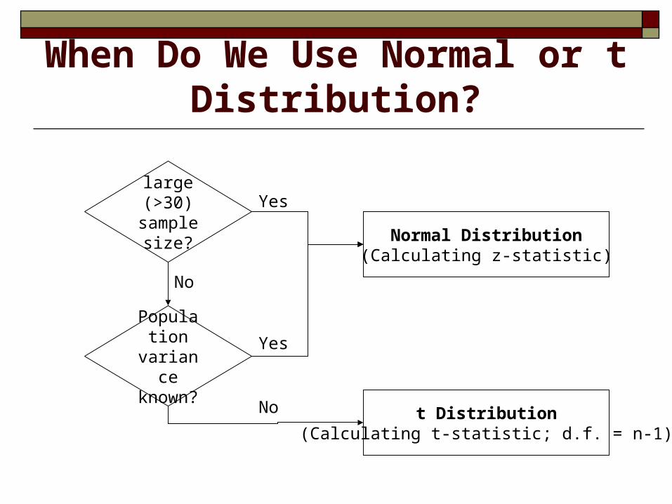
When Do We Use Normal or t Distribution?

large (>30)

sample size?

Population variance known?

Normal Distribution(Calculating z-statistic)

t Distribution(Calculating t-statistic; d.f. = n-1)

Yes

No

No

Yes

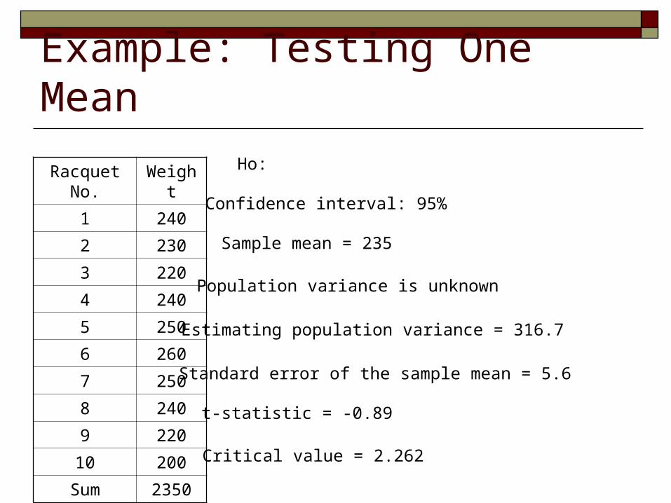
Example: Testing One Mean

Racquet No. Weight

1 240

2 230

3 220

4 240

5 250

6 260

7 250

8 240

9 220

10 200

Sum 2350

Ho:

Confidence interval: 95%

Sample mean = 235

Population variance is unknown

Estimating population variance = 316.7

Standard error of the sample mean = 5.6

t-statistic = -0.89

Critical value = 2.262

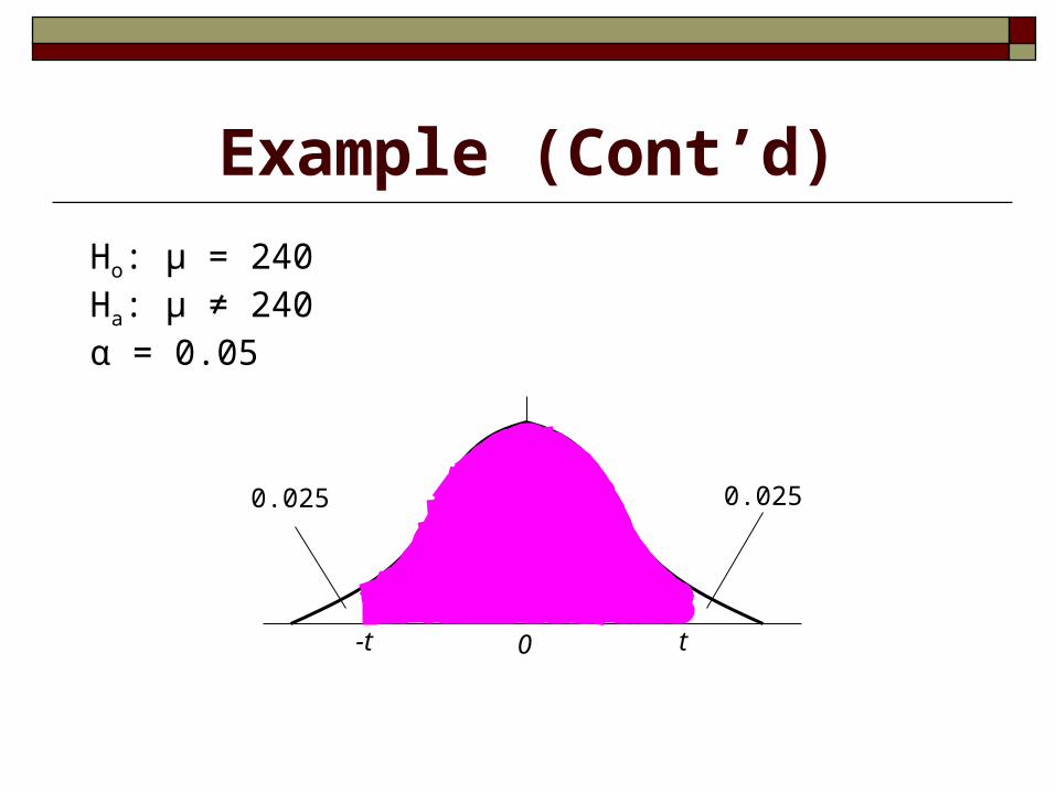
Example (Cont’d)

0

Ho: μ = 240Ha: μ ≠ 240α = 0.05

0.025

t-t

0.025

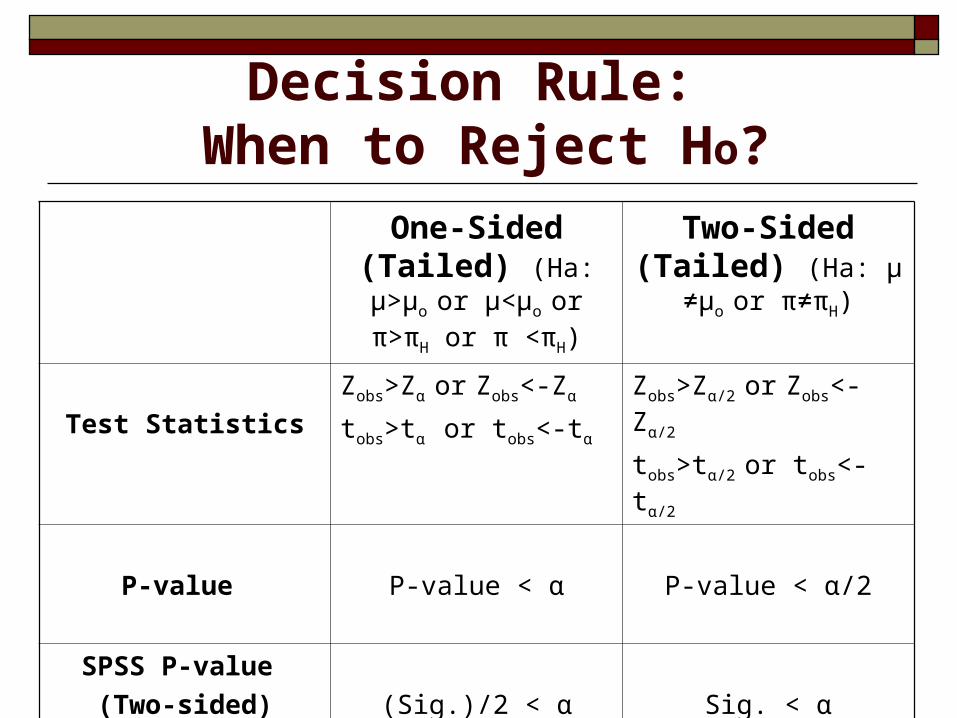
Decision Rule: When to Reject Ho?

One-Sided (Tailed) (Ha: μ>μo or μ<μo or

π>πH or π <πH)

Two-Sided (Tailed) (Ha: μ ≠μo or π≠πH)

Test Statistics

Zobs>Zα or Zobs<-Zα

tobs>tα or tobs<-tα

Zobs>Zα/2 or Zobs<-Zα/2

tobs>tα/2 or tobs<-tα/2

P-value P-value < α P-value < α/2

SPSS P-value

(Two-sided) (Sig.)/2 < α Sig. < α

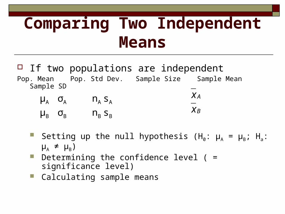
Comparing Two Independent Means

If two populations are independent Pop. Mean Pop. Std Dev. Sample Size Sample Mean Sample SD

μA σA nA sA

μB σB nB sB

Setting up the null hypothesis (H0: μA = μB; Ha: μA ≠ μB) Determining the confidence level ( = significance

level) Calculating sample means

Ax

Bx

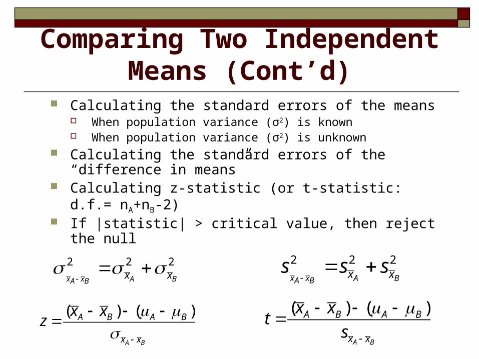
Comparing Two Independent Means (Cont’d)

Calculating the standard errors of the means When population variance (σ2) is known When population variance (σ2) is unknown

Calculating the standard errors of the “difference in means”

Calculating z-statistic (or t-statistic: d.f.= nA+nB-2) If |statistic| > critical value, then reject the null

( ) ( )

A B

A B A B

x x

x xz

( ) ( )

A B

A B A B

x x

x xt

s

2 2 2

x x A BA Bx x

2 2 2

x x A BA Bx xs s s

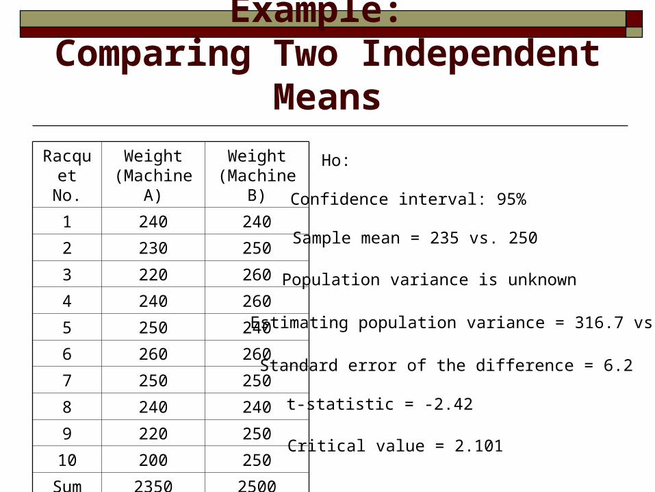
Example: Comparing Two Independent Means

Racquet No.

Weight (Machine A)

Weight (Machine B)

1 240 240

2 230 250

3 220 260

4 240 260

5 250 240

6 260 260

7 250 250

8 240 240

9 220 250

10 200 250

Sum 2350 2500

Ho:

Confidence interval: 95%

Sample mean = 235 vs. 250

Population variance is unknown

Estimating population variance = 316.7 vs. 66.7

Standard error of the difference = 6.2

t-statistic = -2.42

Critical value = 2.101

Example (Cont’d)

0

Ho: µA=µB

Ha: µA≠ µB

α = 0.05

0.025

t-t

0.025

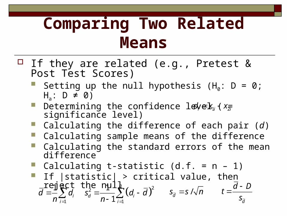
Comparing Two Related Means If they are related (e.g., Pretest & Post Test

Scores) Setting up the null hypothesis (H0: D = 0; Ha: D ≠ 0) Determining the confidence level ( = significance

level) Calculating the difference of each pair (d) Calculating sample means of the difference Calculating the standard errors of the mean

difference Calculating t-statistic (d.f. = n – 1) If |statistic| > critical value, then reject the null

1 2i i id x x

d

d Dt

s

1

1 n

ii

d dn

22

1

1

1

n

d ii

s d dn

/

ds s n

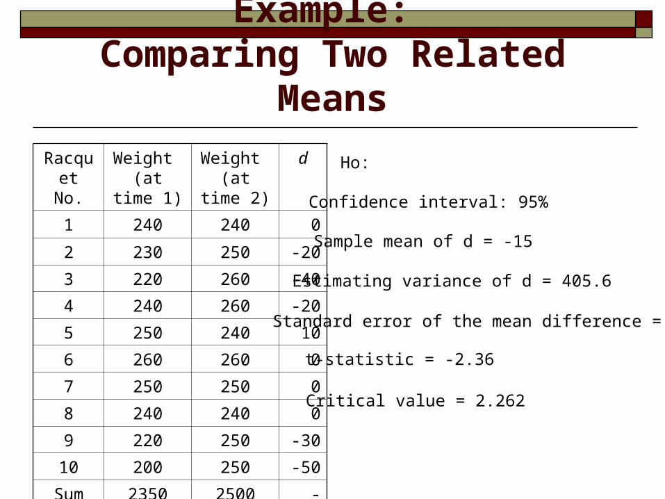
Example: Comparing Two Related Means

Racquet No.

Weight (at time 1)

Weight (at time 2)

d

1 240 240 0

2 230 250 -20

3 220 260 -40

4 240 260 -20

5 250 240 10

6 260 260 0

7 250 250 0

8 240 240 0

9 220 250 -30

10 200 250 -50

Sum 2350 2500 -150

Ho:

Confidence interval: 95%

Sample mean of d = -15

Estimating variance of d = 405.6

Standard error of the mean difference = 6.4

t-statistic = -2.36

Critical value = 2.262

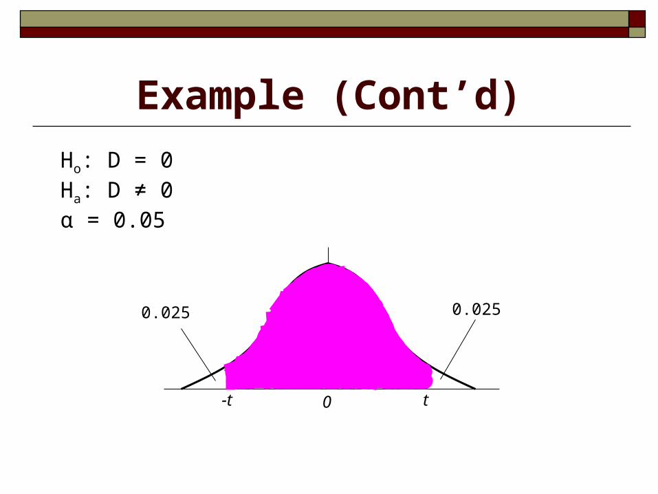
Example (Cont’d)

0

Ho: D = 0Ha: D ≠ 0α = 0.05

0.025

t-t

0.025

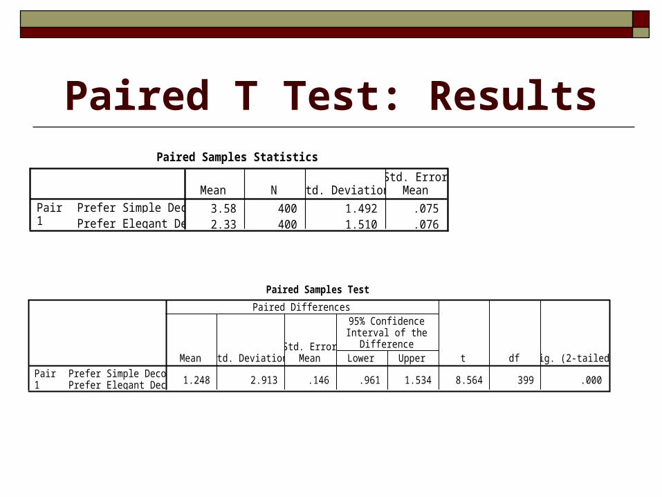
Paired T Test: ResultsPaired Samples Statistics

3.58 400 1.492 .0752.33 400 1.510 .076

Prefer Simple DecorPrefer Elegant Decor

Pair1

Mean N Std. DeviationStd. Error

Mean

Paired Samples Test

1.248 2.913 .146 .961 1.534 8.564 399 .000Prefer Simple Decor -Prefer Elegant Decor

Pair1

Mean Std. DeviationStd. Error

Mean Lower Upper

95% ConfidenceInterval of the

Difference

Paired Differences

t df Sig. (2-tailed)

Decision Rule: When to Reject Ho?

One-Sided (Tailed) (Ha: μ>μo or μ<μo or

π>πH or π <πH)

Two-Sided (Tailed) (Ha: μ ≠μo or π≠πH)

Test Statistics

Zobs>Zα or Zobs<-Zα

tobs>tα or tobs<-tα

Zobs>Zα/2 or Zobs<-Zα/2

tobs>tα/2 or tobs<-tα/2

P-value P-value < α P-value < α/2

SPSS P-value

(Two-sided) (Sig.)/2 < α Sig. < α

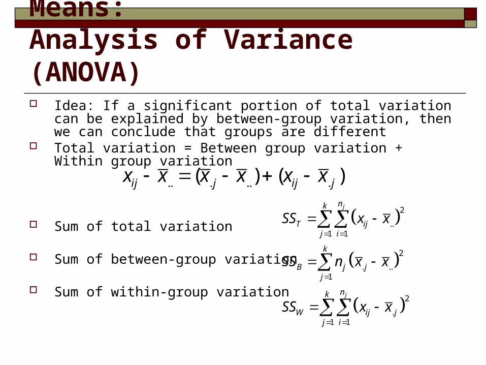
Comparing Three or More Means:Analysis of Variance (ANOVA) Idea: If a significant portion of total variation can be explained by

between-group variation, then we can conclude that groups are different

Total variation = Between group variation + Within group variation

Sum of total variation

Sum of between-group variation

Sum of within-group variation

.. . .. .( ) ( )ij j ij jx x x x x x

2

..1 1

2

. ..1

2

.1 1

j

j

nk

T ijj i

k

B j jj

nk

W ij jj i

SS x x

SS n x x

SS x x

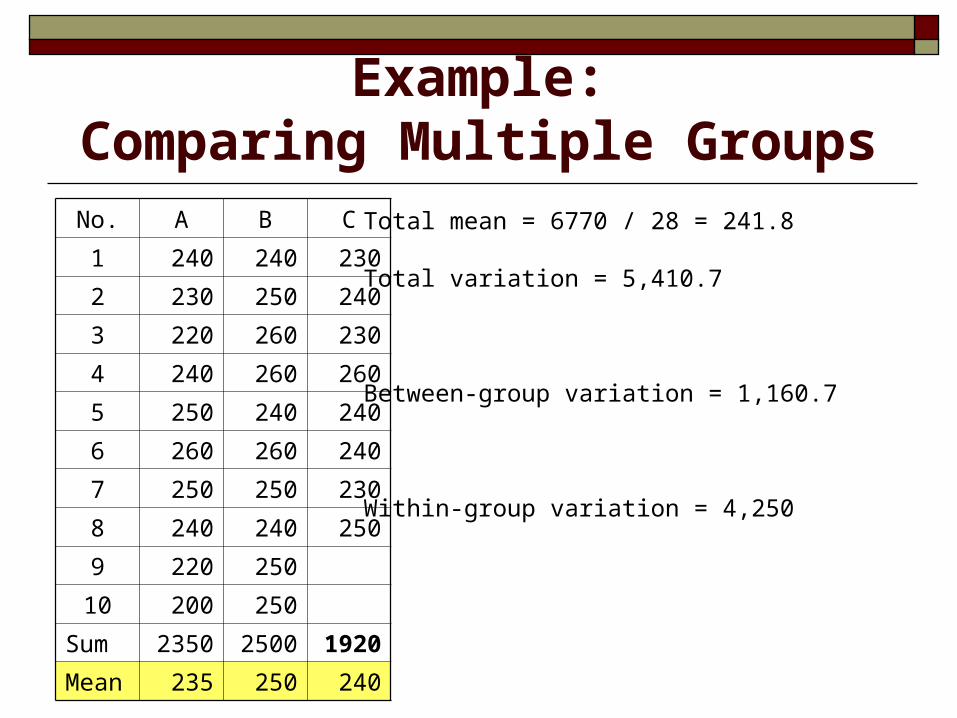
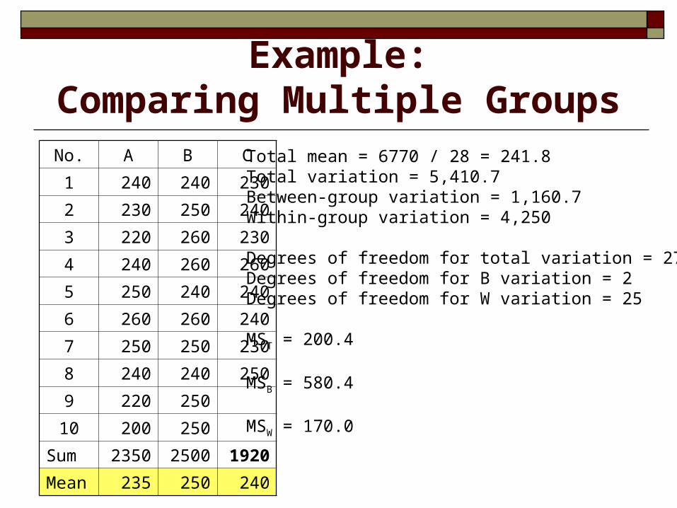
Example:Comparing Multiple Groups

No. A B C

1 240 240 230

2 230 250 240

3 220 260 230

4 240 260 260

5 250 240 240

6 260 260 240

7 250 250 230

8 240 240 250

9 220 250

10 200 250

Sum 2350 2500 1920

Mean 235 250 240

Total mean = 6770 / 28 = 241.8

Total variation = 5,410.7

Between-group variation = 1,160.7

Within-group variation = 4,250

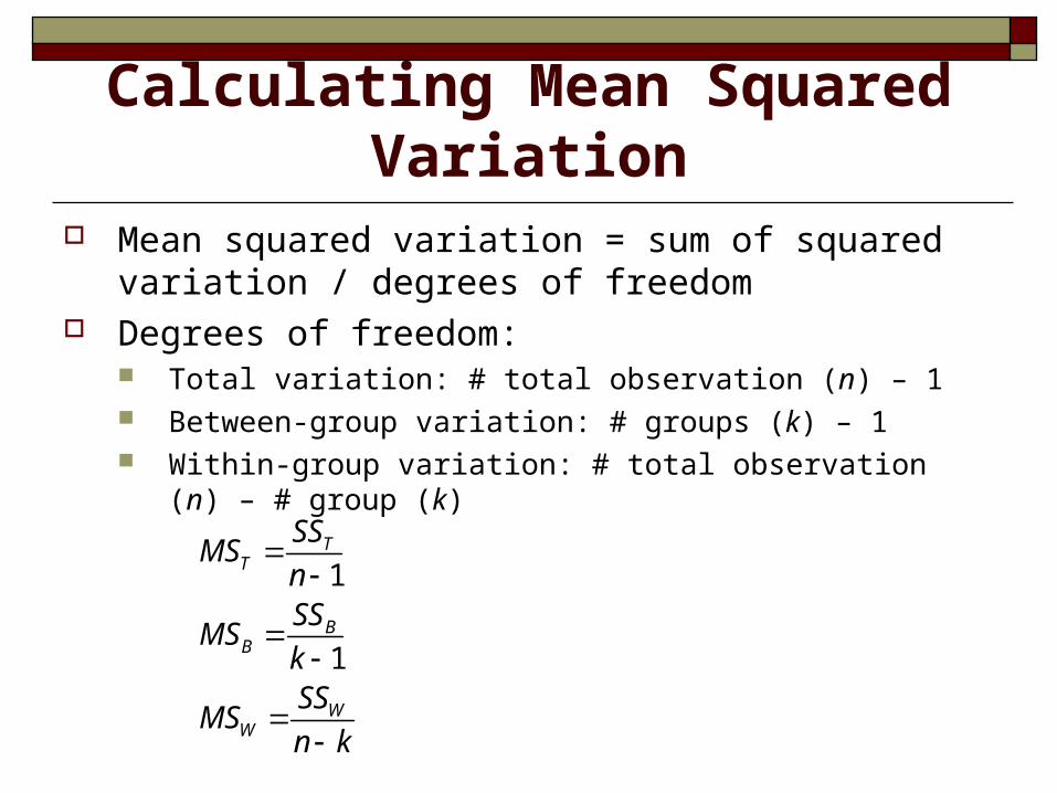
Calculating Mean Squared Variation

Mean squared variation = sum of squared variation / degrees of freedom

Degrees of freedom: Total variation: # total observation (n) – 1 Between-group variation: # groups (k) – 1 Within-group variation: # total observation (n) – # group (k)

1

1

TT

BB

WW

SSMS

nSS

MSkSS

MSn k

Example:Comparing Multiple Groups

No. A B C

1 240 240 230

2 230 250 240

3 220 260 230

4 240 260 260

5 250 240 240

6 260 260 240

7 250 250 230

8 240 240 250

9 220 250

10 200 250

Sum 2350 2500 1920

Mean 235 250 240

Total mean = 6770 / 28 = 241.8Total variation = 5,410.7Between-group variation = 1,160.7Within-group variation = 4,250

Degrees of freedom for total variation = 27Degrees of freedom for B variation = 2Degrees of freedom for W variation = 25

MST = 200.4

MSB = 580.4

MSW = 170.0

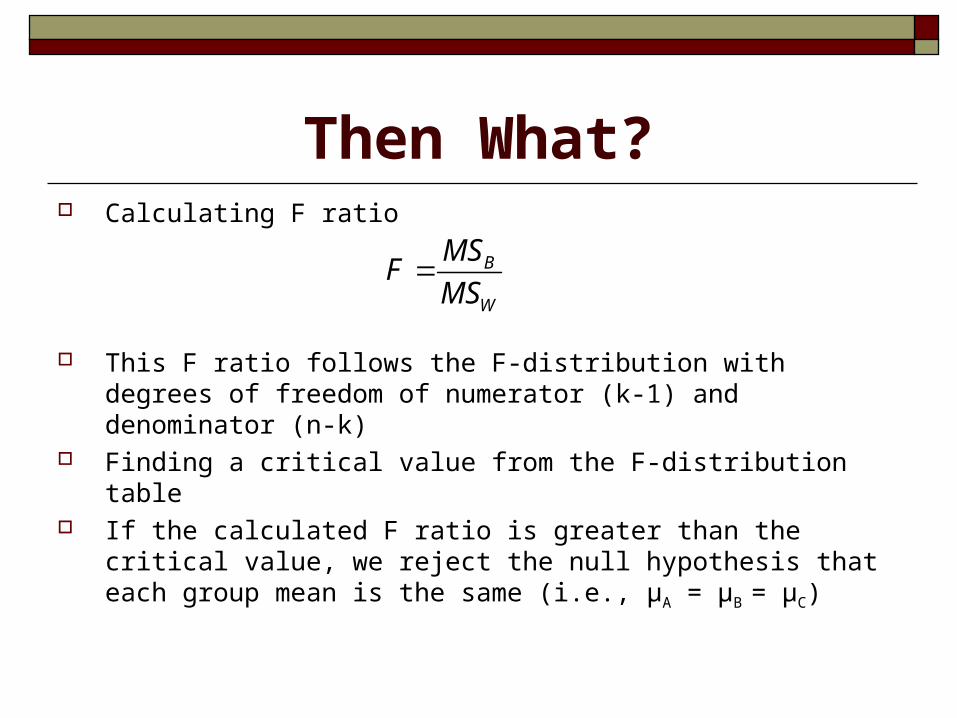
Then What? Calculating F ratio

This F ratio follows the F-distribution with degrees of freedom of numerator (k-1) and denominator (n-k)

Finding a critical value from the F-distribution table If the calculated F ratio is greater than the critical value, we reject

the null hypothesis that each group mean is the same (i.e., μA = μB

= μC)

B

W

MSF

MS

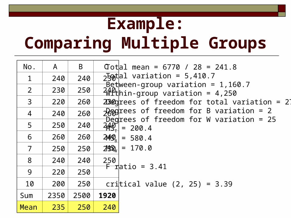
Example:Comparing Multiple Groups

No. A B C

1 240 240 230

2 230 250 240

3 220 260 230

4 240 260 260

5 250 240 240

6 260 260 240

7 250 250 230

8 240 240 250

9 220 250

10 200 250

Sum 2350 2500 1920

Mean 235 250 240

Total mean = 6770 / 28 = 241.8Total variation = 5,410.7Between-group variation = 1,160.7Within-group variation = 4,250Degrees of freedom for total variation = 27Degrees of freedom for B variation = 2Degrees of freedom for W variation = 25MST = 200.4MSB = 580.4MSW = 170.0

F ratio = 3.41

critical value (2, 25) = 3.39

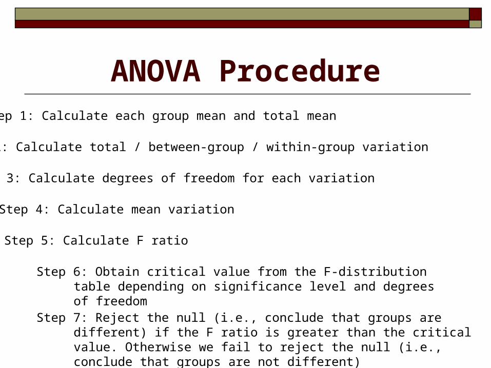
ANOVA ProcedureStep 1: Calculate each group mean and total mean

Step 2: Calculate total / between-group / within-group variation

Step 3: Calculate degrees of freedom for each variation

Step 4: Calculate mean variation

Step 5: Calculate F ratio

Step 6: Obtain critical value from the F-distribution table depending on significance level and degrees of freedom

Step 7: Reject the null (i.e., conclude that groups are different) if the F ratio is greater than the critical value. Otherwise we fail to reject the null (i.e., conclude that groups are not different)

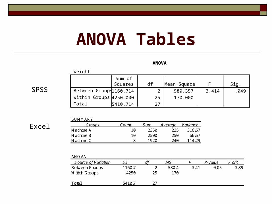
ANOVA TablesANOVA

Weight

1160.714 2 580.357 3.414 .049

4250.000 25 170.000

5410.714 27

Between Groups

Within Groups

Total

Sum ofSquares df Mean Square F Sig.

SPSS

ExcelSUMMARY

Groups Count Sum Average VarianceMachine A 10 2350 235 316.67Machine B 10 2500 250 66.67Machine C 8 1920 240 114.29

ANOVASource of Variation SS df MS F P-value F crit

Between Groups 1160.7 2 580.4 3.41 0.05 3.39Within Groups 4250 25 170

Total 5410.7 27

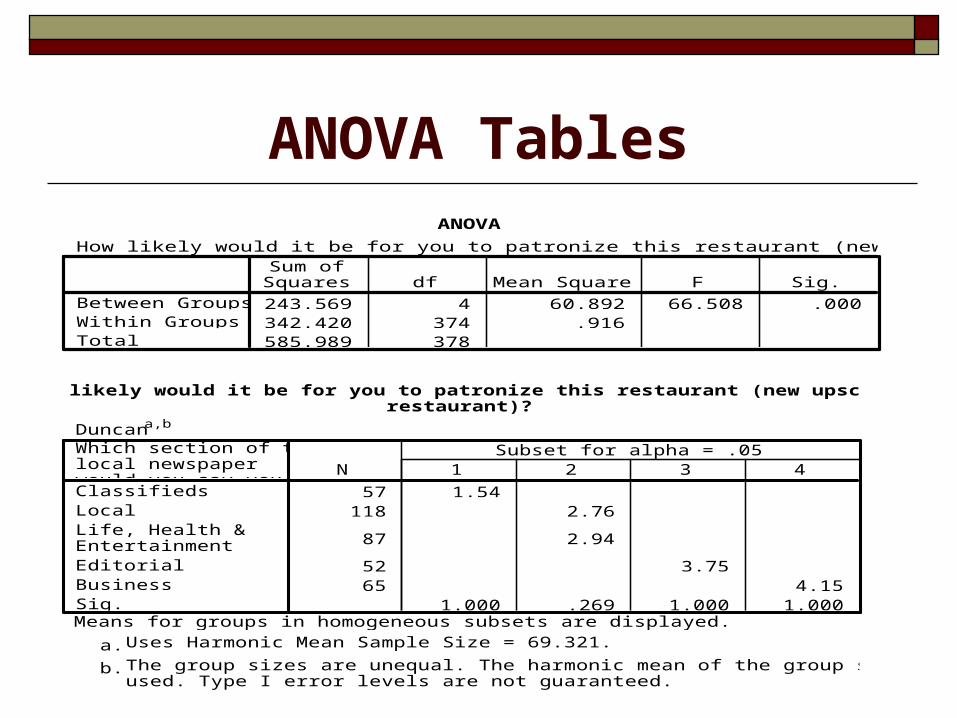
ANOVA TablesANOVA

How likely would it be for you to patronize this restaurant (new upscale restaurant)?

243.569 4 60.892 66.508 .000342.420 374 .916585.989 378

Between GroupsWithin GroupsTotal

Sum ofSquares df Mean Square F Sig.

How likely would it be for you to patronize this restaurant (new upscalerestaurant)?

Duncana,b

57 1.54118 2.76

87 2.94

52 3.7565 4.15

1.000 .269 1.000 1.000

Which section of thelocal newspaperwould you say youread most frequently?ClassifiedsLocalLife, Health &EntertainmentEditorialBusinessSig.

N 1 2 3 4Subset for alpha = .05

Means for groups in homogeneous subsets are displayed.Uses Harmonic Mean Sample Size = 69.321.a.

The group sizes are unequal. The harmonic mean of the group sizes isused. Type I error levels are not guaranteed.

b.

Check Points for ANOVA What is the null hypothesis? Do you measure the difference in what? What is the treatment? Can you calculate total / between-group /

within-group variation? Can you calculate degrees of freedom for each

variation? Can you calculate the F-ratio and find the

critical value from the F-distribution table?

Part 2

Cross Tabulations and Chi-square Analysis

Correlation Analysis

Are Two Variables Associated? Categorical variables (i.e., nominal and ordinal

scales)

Continuous variables (i.e., interval and ratio scales)

Cross TabulationInvestigating contingent relationships…

Are two variables independent?

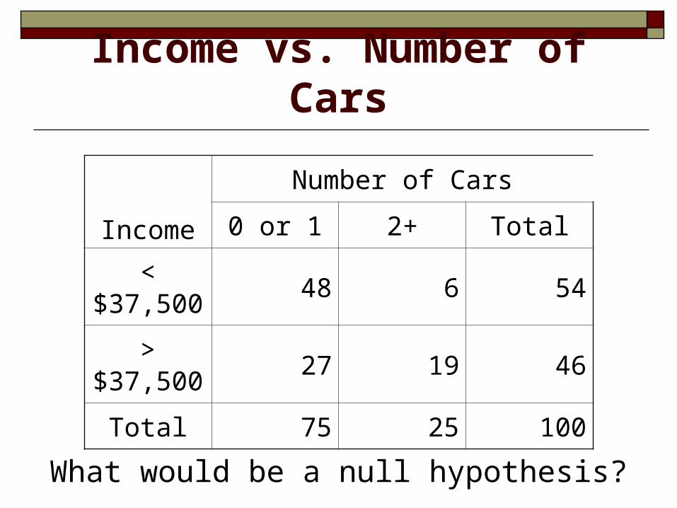
Income vs. Number of Cars

Income

Number of Cars

0 or 1 2+ Total

< $37,500 48 6 54

> $37,500 27 19 46

Total 75 25 100

What would be a null hypothesis?

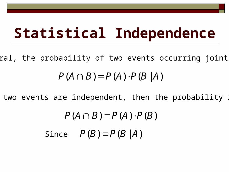
Statistical Independence

In general, the probability of two events occurring jointly is

( ) ( ) ( | )P A B P A P B A

If the two events are independent, then the probability is

( ) ( ) ( )P A B P A P B

Since ( ) ( | )P B P B A

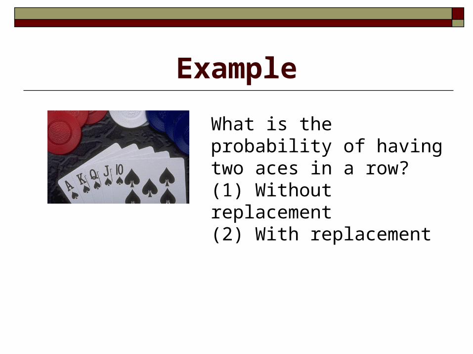
Example

What is the probability of having two aces in a row?(1) Without replacement(2) With replacement

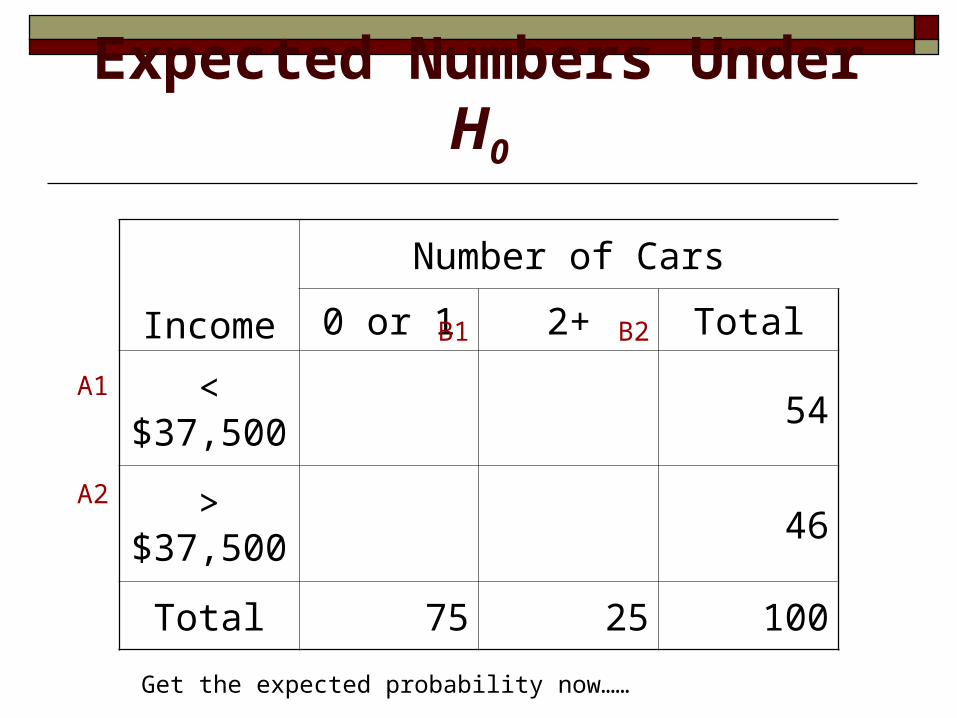
Expected Numbers Under H0

Income

Number of Cars

0 or 1 2+ Total

< $37,500 54

> $37,500 46

Total 75 25 100

A1

A2

B1 B2

Get the expected probability now……

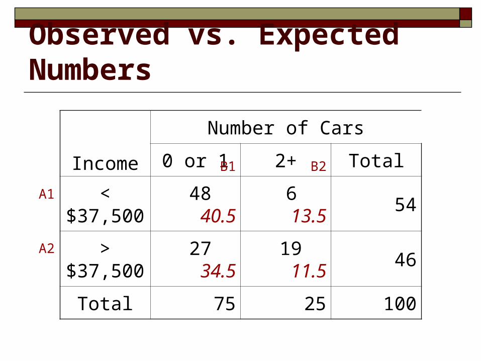
Observed vs. Expected Numbers

Income

Number of Cars

0 or 1 2+ Total

< $37,500 48 40.5 6 13.5 54

> $37,500 27 34.5 19 11.5 46

Total 75 25 100

A1

A2

B1 B2

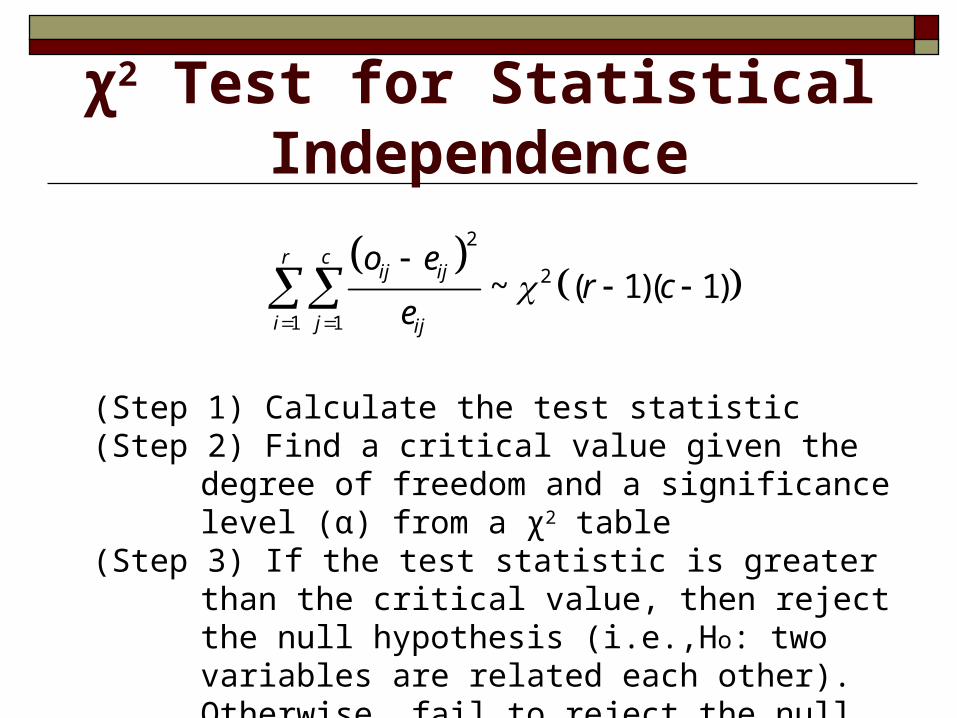
χ2 Test for Statistical Independence

2

2

1 1

~ ( 1)( 1)r c

ij ij

i j ij

o er c

e

(Step 1) Calculate the test statistic(Step 2) Find a critical value given the degree of freedom and

a significance level (α) from a χ2 table(Step 3) If the test statistic is greater than the critical value,

then reject the null hypothesis (i.e.,Ho: two variables are related each other). Otherwise, fail to reject the null (i.e., Ha: two variables are independent)

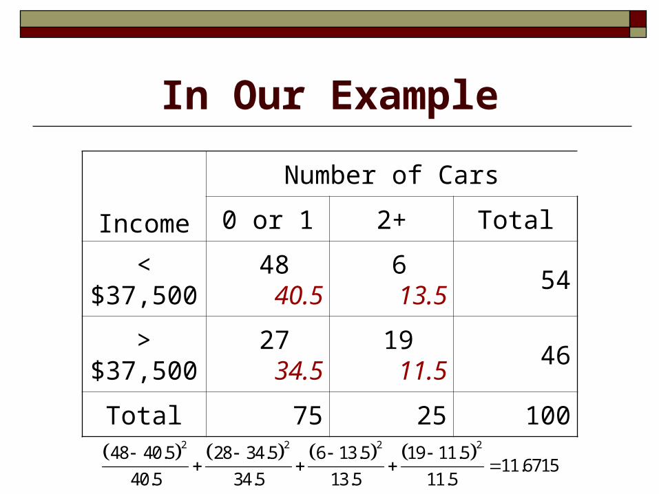
In Our Example

Income

Number of Cars

0 or 1 2+ Total

< $37,500 48 40.5 6 13.5 54

> $37,500 27 34.5 19 11.5 46

Total 75 25 100

2 2 2 248 40.5 28 34.5 6 13.5 19 11.5

11.671540.5 34.5 13.5 11.5

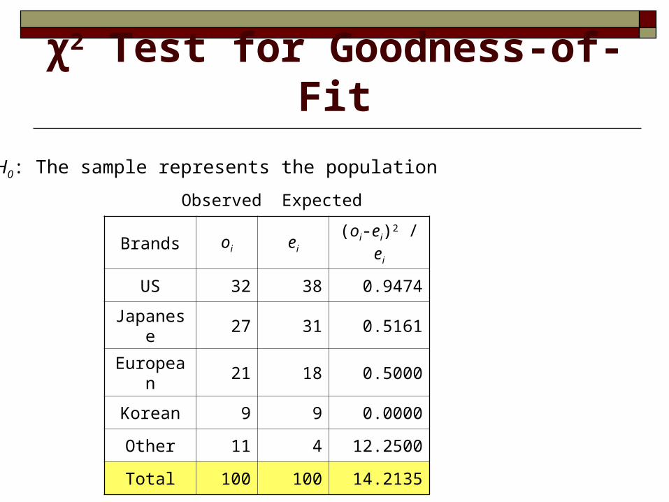
χ2 Test for Goodness-of-Fit

H0: The sample represents the population

Brands oi ei (oi-ei)2 / ei

US 32 38 0.9474

Japanese 27 31 0.5161

European 21 18 0.5000

Korean 9 9 0.0000

Other 11 4 12.2500

Total 100 100 14.2135

Observed Expected

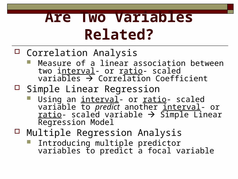
Are Two Variables Related? Correlation Analysis

Measure of a linear association between two interval- or ratio- scaled variables Correlation Coefficient

Simple Linear Regression Using an interval- or ratio- scaled variable to predict

another interval- or ratio- scaled variable Simple Linear Regression Model

Multiple Regression Analysis Introducing multiple predictor variables to predict a

focal variable

Correlation Analysis

X

Y

r = 0.8

X

Y

r = –0.8

X

Y

r = 1.0

X

Y

r = 0

X

Yr = ?

1 1r

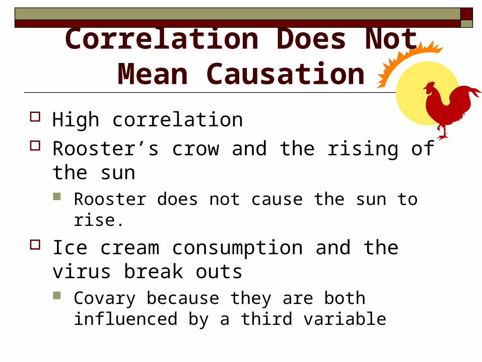
Correlation Does Not Mean Causation

High correlation Rooster’s crow and the rising of the sun

Rooster does not cause the sun to rise. Ice cream consumption and the virus

break outs Covary because they are both influenced by

a third variable

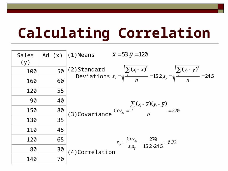
Calculating Correlation

Sales (y) Ad (x)

100 50

160 60

120 55

90 40

150 80

130 35

110 45

120 65

80 30

140 70

(1) Means

(2) StandardDeviations

(3) Covariance

(4) Correlation

53, 120x y

2 2

15.2, 24.5i i

i ix y

x x y ys s

n n

270

i ii

xy

x x y yCov

n

2700.73

15.2 24.5xy

xyx y

Covr

s s

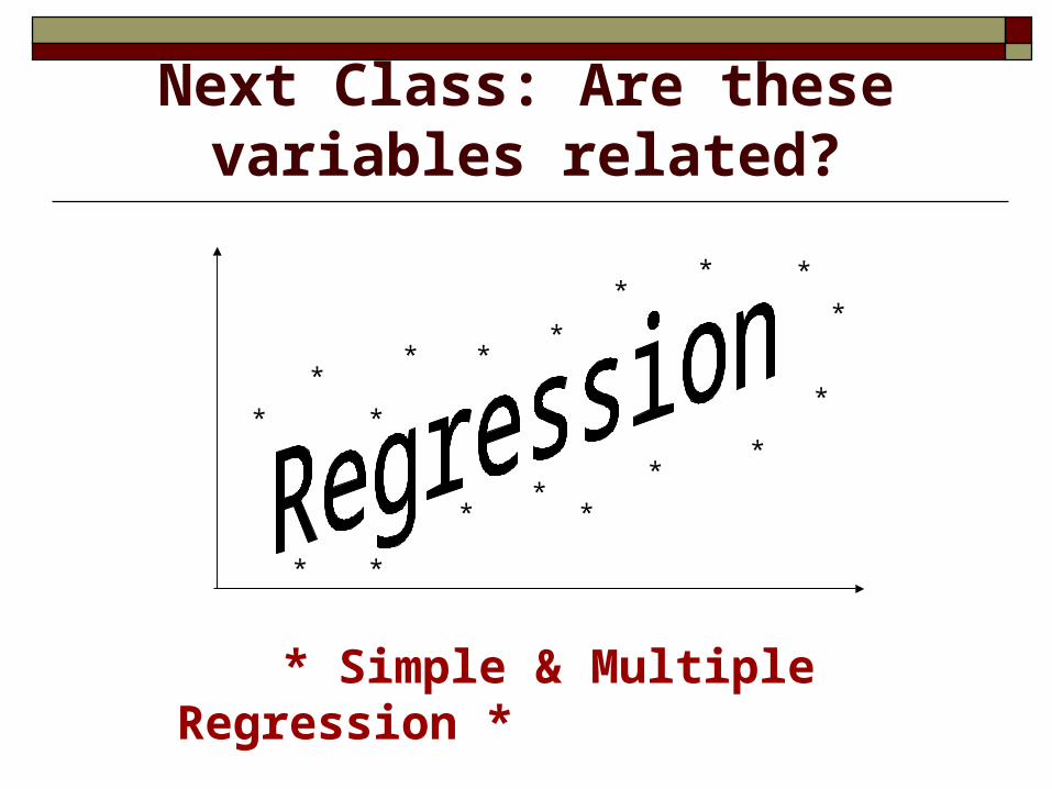
Next Class: Are these variables related?

** *

*

*

**

**

**

*

*

*

*

*

*

*

* Simple & Multiple Regression *