Testing Graphs against an Unknown Distribution*

Lior Gishboliner Asaf Shapira

Abstract

The area of graph property testing seeks to understand the relation between the global properties ofa graph and its local statistics. In the classical model, the local statistics of a graph is defined relative toa uniform distribution over the graph’s vertex set. A graph property P is said to be testable if the localstatistics of a graph can allow one to distinguish between graphs satisfying P and those that are far fromsatisfying it.

Goldreich recently introduced a generalization of this model in which one endows the vertex set of theinput graph with an arbitrary and unknown distribution, and asked which of the properties that can betested in the classical model can also be tested in this more general setting. We completely resolve thisproblem by giving a (surprisingly “clean”) characterization of these properties. To this end, we prove aremoval lemma for vertex weighted graphs which is of independent interest.

1 Introduction

1.1 Background and the main result

Property testers are fast randomized algorithms whose goal is to distinguish (with high probability, say, 2/3)between objects satisfying some fixed property P and those that are ε-far from satisfying it. Here, ε-far meansthat an ε-fraction of the input object should be modified in order to obtain an object satisfying P. The studyof such problems originated in the seminal papers of Rubinfeld and Sudan [28], Blum, Luby and Rubinfeld [9],and Goldreich, Goldwasser and Ron [20]. Problems of this nature have been studied in so many areas that itwill be impossible to survey them here. Instead, the reader is referred to the recent monograph [18] for morebackground and references. While this area studies questions in theoretical computer science, it has severalstrong connections with central problems in extremal combinatorics, most notably to the regularity methodand the removal lemma, see Subsection 1.2.

The classical property testing model assumes that one can uniformly sample entries of the input. Indistribution-free testing, one assumes that the input is endowed with some arbitrary and unknown distributionD, which also affects the way one defines the distance to satisfying a property. As discussed in [19], onemotivation for this model is that it can handle settings in which one cannot produce uniformly distributedentries from the input. Another motivation is that the distribution D can assign higher weight/importanceto parts of the input which we want to have higher impact on the distance to satisfying the given property.Until very recently, problems of this type were studied almost exclusively in the setting of testing propertiesof functions, see [10, 11, 15, 17, 24]. Let us mention that distribution-free testing is similar in spirit to thecelebrated PAC learning model of Valiant [31], see also the discussion in [27].

Our investigation here concerns a distribution-free variant of the adjacency matrix model, also known asthe dense graph model. The adjacency matrix model was first defined and studied in [20], where the area ofproperty testing was first introduced. This model has been extensively studied in the past two decades, seeChapter 8 of [18]. For a selected (but certainly not comprehensive) list of works on the dense graph model ofproperty testing, see [2, 21, 23].

*A preliminary version of this paper has appeared in the Proceedings of STOC ’19.School of Mathematics, Tel Aviv University, Tel Aviv 69978, Israel. Email: liorgis1@post.tau.ac.il. Supported in part by

ERC Starting Grant 633509.School of Mathematics, Tel Aviv University, Tel Aviv 69978, Israel. Email: asafico@tau.ac.il. Supported in part by ISF

Grant 1028/16 and ERC Starting Grant 633509.

1

Instead of defining the adjacency matrix model of [20], let us directly define its distribution-free variantwhich was introduced recently by Goldreich [19]. Since the distribution in this model is over the input’svertices, it is called the Vertex-Distribution-Free (VDF) model1. The input to the algorithm is a graph Gand some arbitrary and unknown distribution D on V (G). We will thus usually refer to the input as the pair(G,D). For a pair of graphs G1, G2 on the same vertex-set V , and for a distribution D on V , the (edit) distancebetween G1 and G2 with respect to D is defined as

∑x,y∈E(G1)4E(G2)D(x)D(y). We say that (G,D) is ε-far

from satisfying a graph property2 P if for every G′ ∈ P, the distance between G and G′ with respect to Dis at least ε. A tester for a graph property P is an algorithm that receives as input a pair (G,D) and aproximity parameter ε, and distinguishes with high probability (say 2

3 ) between the case that G satisfies Pand the case that (G,D) is ε-far from P. The algorithm has access to a device that produces random verticesfrom G distributed according to D. The only3 other way the algorithm can access G is by performing “edgequeries” of the form “is (u, v) an edge of G?”. We say that property P is testable in the VDF model if thereis a function q(ε) and a tester for P that always performs a total number of at most q(ε) vertex samples andedge queries to the input. We stress again that D is unknown to the tester, so (in particular) that q should beindependent of D. The function q is sometimes referred to as the sample (or query) complexity of the tester.A tester has 1-sided error if it always accepts an input satisfying P. Otherwise it has 2-sided error.

Suppose we assume that in the VDF model, the distribution D is restricted to be the uniform distribution;in particular, the distance between n-vertex graphs G,G′ (on the same vertex-set) is |E(G)4E(G′)|/n2, andG is ε-far from P if one needs to change at least εn2 edges to turn G into a graph satisfying P. In this paperwe will refer to this model as the standard model. This model is “basically” equivalent to the adjacency matrixmodel, which was introduced in [20]. We refer the reader to [19] for a discussion on the subtle differencesbetween the adjacency matrix model and the above defined standard model4.

A very elegant result proved in [19], states that if P is testable in the VDF model then it is testable in thestandard model with one-sided error. A natural follow-up question, raised by Goldreich in [19], asks whetherevery property which is testable with one-sided error in the standard model, is also testable in the VDF model.A characterization of the properties testable with one-sided error in the standard model was given in [5], whereit was shown that these are precisely the semi-hereditary properties (see [5] for the definition of this term).We show (see Proposition 4.2), that if P is testable in the VDF model then P is hereditary5. Since thereare properties which are semi-hereditary but not hereditary, this implies a negative answer to Goldreich’squestion. Thus, it is natural to ask the following revised version of Goldreich’s question:

Problem 1.1. Are all hereditary graph properties testable in the VDF model?

It might be natural to guess6 that every hereditary property is testable in the VDF model, the justificationbeing that all lemmas that were used in [5] should also hold for weighted graphs. As it turns out, this is indeedthe case. However, putting all these lemmas together does not seem to work in the VDF model. As our mainresult, Theorem 1 below, shows, it is no coincidence that the proof technique of [5] does not carry over as isto the weighted setting.

We start with an important definition. Let us say that a graph property P is extendable if for every graphG satisfying P there is a graph G′ on |V (G)| + 1 vertices which satisfies P and contains G as an inducedsubgraph. In other words, P is extendable if whenever G is a graph satisfying P and v is a “new” vertex (i.e.v /∈ V (G)), one can connect v to V (G) in such a way that this larger graph will also satisfy P. Note thatif P is extendable then in fact for every graph G ∈ P and for every n > |V (G)|, there is an n-vertex graphsatisfying P which contains G as an induced subgraph. Our main result in this paper is the following:

Theorem 1. A graph property is testable in the VDF model if and only if it is hereditary and extendable.

It is interesting to compare the above (rather) simple characterization of the properties that are testable

1Goldreich suggested to study variants of this model in other settings (such as bounded degree graphs [22]) as well. For brevity,we will use the term “VDF model” to refer to the “VDF variant of the adjacency matrix model”.

2A graph property is simply a family of graphs closed under isomorphism.3Note that the algorithm does not receive |V (G)| as part of the input.4Just as an example, in [20] the tester “knows” |V (G)| while in the VDF model (and thus also in the standard model) it does not.5A graph property is hereditary if it is closed under removal of vertices.6This was at least our initial guess.

2

in the VDF model, with the (very) complicated characterization of [2] of the properties that are testable inthe standard model.

Let us mention some immediate consequences of Theorem 1. Since a graph cannot contain both an isolatedvertex and a vertex connected to all other vertices, we infer that for every fixed H the (hereditary) propertyof being induced H-free is extendable. We thus infer that:

Corollary 2. The property of being induced H-free is testable in the VDF model for every fixed H.

It is also clear that the property of being H-free is extendable if and only if H has no isolated vertices. Wethus infer that:

Corollary 3. The property of being H-free is testable in the VDF model if and only if H has no isolatedvertices.

It is easy to see that most (natural) hereditary graph properties are extendable, so Theorem 1 immediatelyimplies that they are all testable in the VDF model. These include the properties of being Perfect, Interval,Chordal and k-Colorable. In the other direction, Theorem 1 implies that if H has an isolated vertex then H-freeness is not testable in the VDF model. If one is interested in a more “natural” non-extendable hereditaryproperty, then it is not hard to see that another such example is the property P of being induced A,B-free,where A (resp. B) is the graph obtained from the 2-edge path P2 by adding a new vertex which is adjacentto all 3 vertices of P2 (resp. not adjacent to any vertex of P2). It is easy to see that C5 satisfies P but is notextendable. It was proved in [19] that the properties of being Hamiltonian, Eulerian and Connected are nottestable in the VDF model. Those three results follow immediately from our Theorem 1 since these propertiesare not hereditary.

1.2 The combinatorial interpretation of Theorem 1

Let us discuss the combinatorial implications of Theorem 1 and its relation to other results in the area ofextremal combinatorics. The famous triangle removal lemma of Ruzsa and Szemeredi [29] states that if agraph G is ε-far from being triangle free (with respect to the uniform distribution), then a (uniform) sampleof s(ε) vertices from G contains a triangle with probability at least 2

3 . We refer the reader to [13] for morebackground on this lemma and its variants. The result of [5] mentioned above, can be thought of as ageneralization of this lemma to arbitrary hereditary properties. It can be stated as saying that for everyhereditary graph property P there is a function sP : (0, 1)→ N such that the following holds for every ε > 0.If a graph G is ε-far from P (with respect to the uniform distribution) then a (uniform) sample of sP(ε)vertices from G induces a graph not satisfying P with probability at least 2/3.

To prove (the “if” direction of) Theorem 1, we will actually prove the following combinatorial statement,which can be thought of as a vertex-weighted version of the graph removal lemma.

Theorem 4. For every hereditary and extendable graph property P there is a function sP : (0, 1) → N suchthat the following holds for every ε > 0 and for every vertex-weighted graph (G,D) which is ε-far from P.Let u1, . . . , us, s = sP(ε), be a sequence of random vertices of G, sampled according to D and independently.Then G[u1, . . . , us] does not satisfy P with probability at least 2

3 .

The following similar-looking result7 was (implicitly) proved by Austin and Tao [7] and Lovasz and Szegedy [26].

Theorem 5 ([7, 26]). For every hereditary graph property P there is a function sP : (0, 1) → N such thatthe following holds for every ε > 0 and for every vertex-weighted graph (G,D) which is ε-far from P. Letu1, . . . , us, s = sP(ε), be a sequence of random vertices of G, sampled according to D and independently.Construct a graph S on [s] by letting i, j ∈ E(S) if and only if ui, uj ∈ E(G). Then S does not satisfy Pwith probability at least 2

3 .

7We note that the results of [7] and [26] are more general. The authors of [26] actually prove that the conclusion of Theorem5 holds for all graphons. The authors of [7] prove extensions of Theorem 5 in several directions, including a version for uniformhypergraphs, and a strengthening in which the notion of testability is replaced with the stronger notion of repairability.

3

Note that Theorem 5 holds for all hereditary properties, while Theorem 4 only holds for hereditary prop-erties which are extendable. Observe that the graph S in Theorem 5 is a blowup of the graph G[U ], whereU = u1, . . . , us. Thus, the difference between Theorems 4 and 5 is that Theorem 5 only guarantees that ablowup of G[U ] does not satisfy P w.h.p., while Theorem 4 guarantees the stronger assertion that G[U ] itselfdoes not satisfy P w.h.p. This is an important difference: while Theorem 4 immediately implies the existenceof a VDF-tester for every hereditary and extendable property P (see Subsection 3.3), we do not know of anyway of using Theorem 5 to prove the existence of such a tester. One natural candidate for a tester derivedfrom Theorem 5 would be the algorithm which accepts if and only if the graph S (defined in Theorem 5) doesnot satisfy P. It turns out, however, that this algorithm often fails to be a valid tester8.

It is worth noting that Theorem 5 can be deduced from the “unweighted” case, i.e. the result of [5], via asimple argument, see Lemma 5.5 and the discussion following it. On the other hand, the proof of Theorem 4requires several new ideas on top of those used in [5].

1.3 Variants of the VDF model

The proof of the “only if” part of Theorem 1, showing that if P is either non-extendable or non-hereditary thenP is not testable in the VDF model, relies on allowing the input graph to have only O(1) vertices (where theconstant is independent of ε); on excluding |V (G)| from the input fed to the tester; and on having distributionsD that assign to some vertices weight Θ(1) and to some vertices weight o(1/|V (G)|). This raises the naturalquestion of what happens if we only require the tester to work on sufficiently large graphs; or if the testerreceives |V (G)| as part of the input; or if we forbid D from assigning very low or very high weights (as above).As the following four theorems show, either one of these variations has a dramatic effect on the model, sinceit then allows all hereditary properties to be testable.

We start with the setting in which the input graph is guaranteed to be large enough. In a revised versionof [19], Goldreich asked whether every hereditary property P is testable (in the VDF model) on graphs oforder at least M = MP , for M which is independent of ε. As we show in Proposition 5.2, this turns out to befalse. On the positive side, we show that under the stronger assumption that the input size is at least MP(ε)(where MP : (0, 1)→ N is a function dependent on P), all hereditary properties are testable.

Theorem 6. Under the promise that |V (G)| 1, every hereditary property is testable with one-sided errorin the VDF model.

D. Ron (personal communication) asked what happens if we allow testers to receive |V (G)| (i.e., the numberof vertices in the input graph) as part of the input9. Our following theorem answers this question.

Theorem 7. If testers can receive |V (G)| as part of the input, then every hereditary property is testable withone-sided error in the VDF model.

Finally, we consider settings in which restrictions are posed on the weights that the distribution D can assign.

Theorem 8. Under the promise that maxv∈V (G)D(v) = o(1), every hereditary property is testable with one-sided error in the VDF model.

Theorem 9. Under the promise that minv∈V (G)D(v) = Ω (1/|V (G)|), every hereditary property is testablewith one-sided error in the VDF model.

We note that the implied constant in the Ω-notation in Theorem 9 is allowed to depend on ε. We refer thereader to Section 5 for the precise statements of Theorems 6–9. Let us mention that the proofs of Theorems 6,7 and 9 rely on reductions to our main result in this paper, Theorem 1. The proof of Theorem 8 proceeds bya reduction to the standard model (i.e. to the result of [5]). As part of this proof, we solve another problemraised in [19].

8For example, if P = C5-freeness then this tester will reject w.h.p if the input graph is a triangle with uniform vertexdistribution (as the graph S will typically contain the 2-blowup of a triangle, and thus contain a copy of C5), even though thisinput graph clearly satisfies P.

9We note that in the VDF model as defined in [19], the number of vertices in the input graph is not known to the tester

4

1.4 Paper overview

The rest of the paper is organized as follows. Section 2 is devoted to proving vertex-weighted analogues ofseveral lemmas that were used in prior works (most notably regularity and counting lemmas, and corollariesthereof). Some more routine parts of these proofs are deferred to the appendix. In Section 3 we prove the“if” direction of Theorem 1 (i.e. Theorem 4). This is by far the most challenging (and interesting) part ofthis paper. The main step towards proving Theorem 1 is establishing Lemma 3.1, which is the key lemma ofthis paper. For the reader’s convenience, we give in Subsection 3.1 an overview of the key ideas of the proof.As the proofs in Section 2 are somewhat routine, we encourage readers who are familiar with the regularitymethod to skip Section 2 (at least on their first read), and go directly to Section 3.

The “only if” direction of Theorem 1 is proved in Section 4. In Section 5 we prove Theorems 6, 7, 8 and9. We also raise two additional problems related to the VDF model; one is to what extent can one extendthe results of Theorems 6-9 beyond hereditary properties, and the other asks if the sample complexity in theVDF model is the same as in the standard model (for properties that are testable in the VDF model), seeSubsection 5.3. Along the way we resolve another open problem raised in [19] (see Lemma 5.5). Throughoutthe paper, when we say that a function is increasing/decreasing we mean weakly increasing/decreasing (i.e.non-decreasing/non-increasing).

2 Preliminary Lemmas

In this section we introduce vertex-weighted analogues of some key tools of the regularity method, most notableSzemeredi’s regularity lemma [30], the strong regularity lemma [1], and the counting lemma, as well as somestandard corollaries thereof. We also prove some other auxiliary lemmas needed for the proof of Theorem 1.

We start with two simple lemmas regarding probability distributions10 on a finite set. Given a distributionD on a set U and a subset W ⊆ U , we use the notation D(W ) :=

∑w∈W D(w), and call D(W ) the weight of

W . We denote by DW the distribution D conditioned on W , namely DW (w) = D(w)D(W ) for every w ∈W .

Lemma 2.1. For every set U , for every η ∈ (0, 1) and for every distribution D on U , there is a partition Pof U into d1/ηe parts such that

∑W∈P

∑x,y∈(W2 )D(x)D(y) ≤ η.

Proof. Let P be a random partition of U into k := d1/ηe parts, where each element is assigned to one of theparts uniformly at random and independently of all other elements. Then for every pair of distinct elementsx, y ∈ U , the probability that x and y belong to the same part is exactly 1

k . By linearity of expectation we have

E

∑W∈P

∑x,y∈(W2 )

D(x)D(y)

=∑

x,y∈(U2)

D(x)D(y) · 1

k<

1

2· 1

k< η,

so there is a choice of P with the required property.

Lemma 2.2. Let a > 0 be an integer, let U be a finite set and let D be a distribution on U such that D(u) ≤ 12a

for every u ∈ U . Then there is a partition U = U1 ∪ · · · ∪ Ua such that D(Ui) ≥ 12a for every 1 ≤ i ≤ a.

Proof. We proof is by induction on a. The base case a = 1 is trivial, so we assume from now on that a ≥ 2.Let U1 ⊆ U be a set of minimal size satisfying D(U1) ≥ 1

2a . Then D(U1) ≤ 1a , because otherwise we could

remove an arbitrary element of U1 (whose weight by assumption is at most 12a ) and thus get a proper subset

of U1 having weight at least 12a , in contradiction the minimality of U1. Now set U ′ := U \ U1, noting that

D(U ′) ≥ 1− 1a . Then every u ∈ U ′ satisfies

DU ′(u) =D(u)

D(U ′)≤

12a

1− 1a

=1

2(a− 1).

10Throughout the paper, we will simply write “distribution” to mean “probability distribution”.

5

So by the induction hypothesis for (U ′,DU ′), there is a partition U ′ = U2 ∪ · · · ∪ Ua such that

D(Ui) = DU ′(Ui) · D(U ′) ≥ 1

2(a− 1)· D(U ′) ≥ 1

2(a− 1)·(

1− 1

a

)=

1

2a

for every 2 ≤ i ≤ a. This completes the proof.

We consider vertex-weighted graphs, i.e. pairs (G,D) such that G is a graph and D is a distribution onV (G). For a set X ⊆ V (G), the subgraph of (G,D) induced by X is defined to be (G[X],DX), where DX isthe distribution D conditioned on X. The weight of an edge/non-edge x, y (with respect to D) is definedas D(x)D(y). For a pair of disjoint sets X,Y ⊆ V (G) with D(X),D(Y ) > 0, the density of (X,Y ) is denotedby d(X,Y ) and defined to be d(X,Y ) = 1

D(X)D(Y )

∑(x,y)∈E(X,Y )D(x)D(y), where E(X,Y ) is the set of edges

with one endpoint in X and one endpoint in Y . If D(X) = 0 or D(Y ) = 0 then define d(X,Y ) = 0. A pairof disjoint vertex-sets (X,Y ) is called ε-regular if for every X ′ ⊆ X and Y ′ ⊆ Y with D(X ′) ≥ εD(X) andD(Y ′) ≥ εD(Y ), it holds that |d(X ′, Y ′)− d(X,Y )| ≤ ε. The following lemma describes some basic propertiesof ε-regular pairs.

Lemma 2.3. Let (G,D) be a vertex-weighted graph, and let X,Y ⊆ V (G) be disjoint vertex-sets such thatD(X),D(Y ) > 0, and such that the pair (X,Y ) is ε-regular with density d. Then the following holds.

1. For every α ≥ ε and X ′ ⊆ X, Y ′ ⊆ Y with D(X ′) ≥ αD(X) and D(Y ′) ≥ αD(Y ), the pair (X ′, Y ′) hasdensity at least d− ε and at most d+ ε, and is ε′-regular with ε′ = maxε/α, 2ε.

2. The set of vertices x ∈ X which satisfy |d(x, Y )− d| > ε has weight less than 2ε · D(X).

Proof. Starting with Item 1, let X ′ ⊆ X and Y ′ ⊆ Y be such that D(X ′) ≥ αD(X) and D(Y ′) ≥ αD(Y ).Since α ≥ ε, the ε-regularity of (X,Y ) implies that d− ε ≤ d(X ′, Y ′) ≤ d+ ε. Now let us show that (X ′, Y ′)is ε′-regular with ε′ = maxε/α, 2ε. Let X ′′ ⊆ X ′ and Y ′′ ⊆ Y ′ be such that D(X ′′) ≥ ε′D(X ′) andD(Y ′′) ≥ ε′D(Y ′). Then D(X ′′) ≥ ε

αD(X ′) ≥ εD(X) and similarly D(Y ′′) ≥ εD(Y ). So by the ε-regularity of(X,Y ) we have |d(X ′′, Y ′′)− d(X,Y )| ≤ ε and hence |d(X ′′, Y ′′)− d(X ′, Y ′)| ≤ 2ε ≤ ε′, as required.

We now prove Item 2. Let X+ (resp. X−) be the set of all x ∈ X satisfying d(x, Y ) > d + ε (resp.d(x, Y ) < d− ε). We have

d(X+, Y ) =1

D(X+)D(Y )·∑x∈X+

∑y∈NY (x)

D(x)D(y) =1

D(X+)D(Y )·∑x∈X+

D(x) · D(Y ) · d(x, Y )

>1

D(X+)D(Y )· D(X+)D(Y ) · (d+ ε) = d+ ε.

So unless D(X+) < εD(X), we get a contradiction to the ε-regularity of (X,Y ). Similarly, we must haveD(X−) < εD(X). The assertion follows.

The following is a vertex-weighted counting lemma.

Lemma 2.4 (Counting lemma for vertex-weighted graphs). For every integer h ≥ 2 and η ∈ (0, 1) there isδ = δ2.4(h, η) such that the following holds. Let H be a graph on [h] and let U1, . . . , Uh be pairwise-disjointvertex-sets in a vertex-weighted graph (G,D), such that the following holds.

1. For every 1 ≤ i < j ≤ h, if i, j ∈ E(H) then d(Ui, Uj) ≥ η, and if i, j /∈ E(H) then d(Ui, Uj) ≤ 1−η.

2. For every 1 ≤ i < j ≤ h, the pair (Ui, Uj) is δ-regular.

Let U be the set of all (u1, . . . , uh) ∈ U1 × · · · × Uh such that u1, . . . , uh induce a copy of H in which ui plays

the role of i for every 1 ≤ i ≤ h. Then∑

(u1,...,uh)∈U∏hi=1D(ui) ≥ δ

∏hi=1D(Ui).

6

Proof. If D(Ui) = 0 for some 1 ≤ i ≤ h then there is nothing to prove, so suppose that D(Ui) > 0 for every1 ≤ i ≤ h. The proof is by induction on h. The base case h = 2 trivially holds with δ = δ(2, η) = η. So fromnow on we assume that h ≥ 3, and set

δ = δ(h, η) = min

1

4(h− 1),η

2,

1

2·(η

2

)h−1

· δ(h− 1, η/2)

.

For each 2 ≤ i ≤ h, let Wi be the set of all vertices u1 ∈ U1 for which |d(u1, Ui) − d(U1, Ui)| > δ. By

Item 2 of Lemma 2.3, we have D(Wi) < 2δ · D(U1). Hence, the set U ′1 := U1 \⋃hi=2Wi satisfies D(U ′1) >

D(U1) − (h − 1) · 2δ · D(U1) ≥ 12D(U1), where in the last inequality we used our choice of δ. Now fix any

u1 ∈ U ′1. We define sets U ′2, . . . , U′h as follows: for 2 ≤ i ≤ h, if 1, i ∈ E(H) then set U ′i = NUi(u1),

and if 1, i /∈ E(H) then set U ′i = Ui \ NUi(u1). By using Item 1 and the fact that u1 ∈ U ′1, we get thatD(U ′i) ≥ (η− δ)D(Ui) ≥ η

2 · D(Ui) for every 2 ≤ i ≤ h. By Item 1 of Lemma 2.3, and by Conditions 1-2 of thecurrent lemma, we get that for every 2 ≤ i < j ≤ h, the pair (U ′i , U

′j) is δ′-regular with δ′ = 2δ/η ≤ δ(h−1, η/2),

and that if i, j ∈ E(H) then d(U ′i , U′j) ≥ η−δ ≥ η/2 and if i, j /∈ E(H) then d(U ′i , U

′j) ≤ 1−η+δ ≤ 1− η

2 .

We now see that the sets U ′2, . . . , U′h satisfy the requirements of the lemma with respect to the graph

H ′ = H[2, . . . , h] and with η2 in place of η. Let U ′ be the set of all (u2, . . . , uh) ∈ U ′2 × · · · × U ′h such that

u2, . . . , uh induce a copy of H ′ with ui playing the role of i for every 2 ≤ i ≤ h. By the induction hypothesis,we have

∑(u2,...,uh)∈U ′

h∏i=2

D(ui) ≥ δ(h− 1, η/2) ·h∏i=2

D(U ′i) ≥ δ(h− 1, η/2) · (η/2)h−1 ·h∏i=2

D(Ui) ≥ 2δ

h∏i=2

D(Ui).

For every (u2, . . . , uh) ∈ U ′, the tuple (u1, . . . , uh) induces a copy of H with ui playing the role of i for every1 ≤ i ≤ h. Hence, for every (u2, . . . , uh) ∈ U ′ we have (u1, . . . , uh) ∈ U (where U is defined in the statementof the lemma). Since this is true for every u1 ∈ U ′1, we get that

∑(u1,...,uh)∈U

h∏i=1

D(ui) ≥∑u1∈U ′

1

D(u1) · 2δh∏i=2

D(Ui) = D(U ′1) · 2δh∏i=2

D(Ui) ≥ δh∏i=1

D(Ui),

as required.

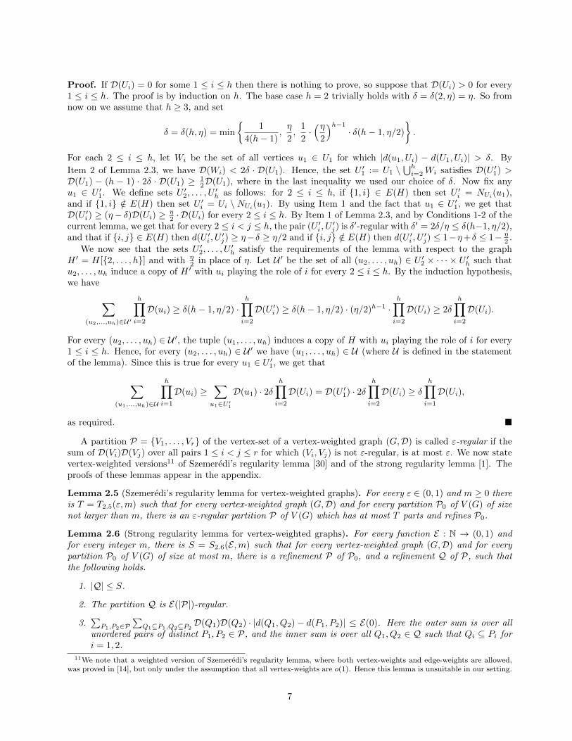
A partition P = V1, . . . , Vr of the vertex-set of a vertex-weighted graph (G,D) is called ε-regular if thesum of D(Vi)D(Vj) over all pairs 1 ≤ i < j ≤ r for which (Vi, Vj) is not ε-regular, is at most ε. We now statevertex-weighted versions11 of Szemeredi’s regularity lemma [30] and of the strong regularity lemma [1]. Theproofs of these lemmas appear in the appendix.

Lemma 2.5 (Szemeredi’s regularity lemma for vertex-weighted graphs). For every ε ∈ (0, 1) and m ≥ 0 thereis T = T2.5(ε,m) such that for every vertex-weighted graph (G,D) and for every partition P0 of V (G) of sizenot larger than m, there is an ε-regular partition P of V (G) which has at most T parts and refines P0.

Lemma 2.6 (Strong regularity lemma for vertex-weighted graphs). For every function E : N → (0, 1) andfor every integer m, there is S = S2.6(E ,m) such that for every vertex-weighted graph (G,D) and for everypartition P0 of V (G) of size at most m, there is a refinement P of P0, and a refinement Q of P, such thatthe following holds.

1. |Q| ≤ S.

2. The partition Q is E(|P|)-regular.

3.∑P1,P2∈P

∑Q1⊆P1,Q2⊆P2

D(Q1)D(Q2) · |d(Q1, Q2)− d(P1, P2)| ≤ E(0). Here the outer sum is over allunordered pairs of distinct P1, P2 ∈ P, and the inner sum is over all Q1, Q2 ∈ Q such that Qi ⊆ Pi fori = 1, 2.

11We note that a weighted version of Szemeredi’s regularity lemma, where both vertex-weights and edge-weights are allowed,was proved in [14], but only under the assumption that all vertex-weights are o(1). Hence this lemma is unsuitable in our setting.

7

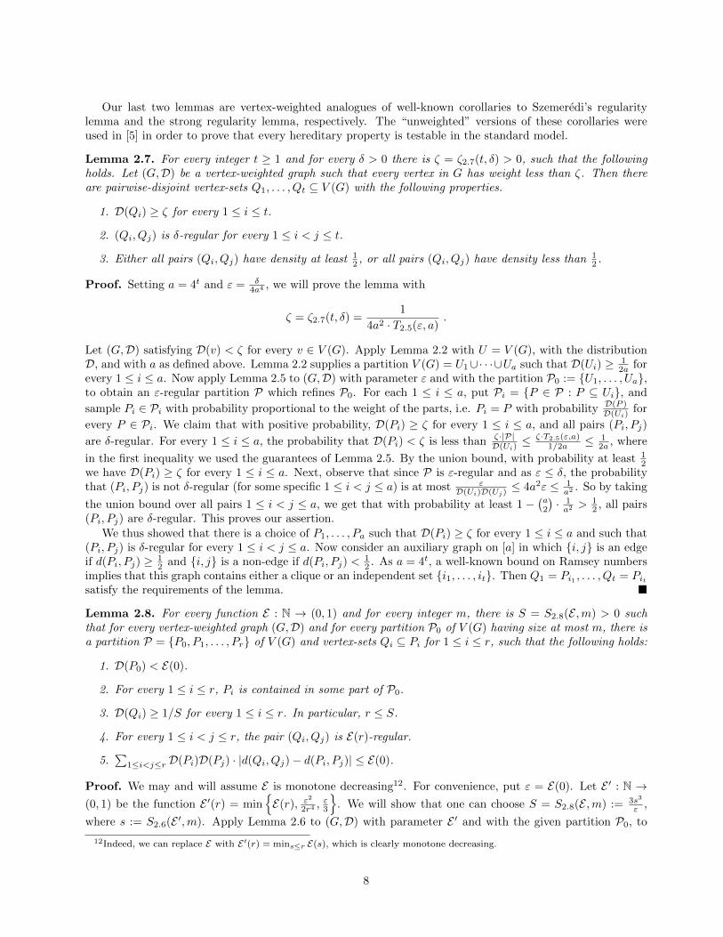
Our last two lemmas are vertex-weighted analogues of well-known corollaries to Szemeredi’s regularitylemma and the strong regularity lemma, respectively. The “unweighted” versions of these corollaries wereused in [5] in order to prove that every hereditary property is testable in the standard model.

Lemma 2.7. For every integer t ≥ 1 and for every δ > 0 there is ζ = ζ2.7(t, δ) > 0, such that the followingholds. Let (G,D) be a vertex-weighted graph such that every vertex in G has weight less than ζ. Then thereare pairwise-disjoint vertex-sets Q1, . . . , Qt ⊆ V (G) with the following properties.

1. D(Qi) ≥ ζ for every 1 ≤ i ≤ t.

2. (Qi, Qj) is δ-regular for every 1 ≤ i < j ≤ t.

3. Either all pairs (Qi, Qj) have density at least 12 , or all pairs (Qi, Qj) have density less than 1

2 .

Proof. Setting a = 4t and ε = δ4a4 , we will prove the lemma with

ζ = ζ2.7(t, δ) =1

4a2 · T2.5(ε, a).

Let (G,D) satisfying D(v) < ζ for every v ∈ V (G). Apply Lemma 2.2 with U = V (G), with the distributionD, and with a as defined above. Lemma 2.2 supplies a partition V (G) = U1∪· · ·∪Ua such that D(Ui) ≥ 1

2a forevery 1 ≤ i ≤ a. Now apply Lemma 2.5 to (G,D) with parameter ε and with the partition P0 := U1, . . . , Ua,to obtain an ε-regular partition P which refines P0. For each 1 ≤ i ≤ a, put Pi = P ∈ P : P ⊆ Ui, and

sample Pi ∈ Pi with probability proportional to the weight of the parts, i.e. Pi = P with probability D(P )D(Ui)

for

every P ∈ Pi. We claim that with positive probability, D(Pi) ≥ ζ for every 1 ≤ i ≤ a, and all pairs (Pi, Pj)

are δ-regular. For every 1 ≤ i ≤ a, the probability that D(Pi) < ζ is less than ζ·|P|D(Ui)

≤ ζ·T2.5(ε,a)1/2a ≤ 1

2a , where

in the first inequality we used the guarantees of Lemma 2.5. By the union bound, with probability at least 12

we have D(Pi) ≥ ζ for every 1 ≤ i ≤ a. Next, observe that since P is ε-regular and as ε ≤ δ, the probabilitythat (Pi, Pj) is not δ-regular (for some specific 1 ≤ i < j ≤ a) is at most ε

D(Ui)D(Uj)≤ 4a2ε ≤ 1

a2 . So by taking

the union bound over all pairs 1 ≤ i < j ≤ a, we get that with probability at least 1−(a2

)· 1a2 >

12 , all pairs

(Pi, Pj) are δ-regular. This proves our assertion.

We thus showed that there is a choice of P1, . . . , Pa such that D(Pi) ≥ ζ for every 1 ≤ i ≤ a and such that(Pi, Pj) is δ-regular for every 1 ≤ i < j ≤ a. Now consider an auxiliary graph on [a] in which i, j is an edgeif d(Pi, Pj) ≥ 1

2 and i, j is a non-edge if d(Pi, Pj) <12 . As a = 4t, a well-known bound on Ramsey numbers

implies that this graph contains either a clique or an independent set i1, . . . , it. Then Q1 = Pi1 , . . . , Qt = Pitsatisfy the requirements of the lemma.

Lemma 2.8. For every function E : N → (0, 1) and for every integer m, there is S = S2.8(E ,m) > 0 suchthat for every vertex-weighted graph (G,D) and for every partition P0 of V (G) having size at most m, there isa partition P = P0, P1, . . . , Pr of V (G) and vertex-sets Qi ⊆ Pi for 1 ≤ i ≤ r, such that the following holds:

1. D(P0) < E(0).

2. For every 1 ≤ i ≤ r, Pi is contained in some part of P0.

3. D(Qi) ≥ 1/S for every 1 ≤ i ≤ r. In particular, r ≤ S.

4. For every 1 ≤ i < j ≤ r, the pair (Qi, Qj) is E(r)-regular.

5.∑

1≤i<j≤r D(Pi)D(Pj) · |d(Qi, Qj)− d(Pi, Pj)| ≤ E(0).

Proof. We may and will assume E is monotone decreasing12. For convenience, put ε = E(0). Let E ′ : N →(0, 1) be the function E ′(r) = min

E(r), ε

2

2r4 ,ε3

. We will show that one can choose S = S2.8(E ,m) := 3s3

ε ,

where s := S2.6(E ′,m). Apply Lemma 2.6 to (G,D) with parameter E ′ and with the given partition P0, to

12Indeed, we can replace E with E ′(r) = mins≤r E(s), which is clearly monotone decreasing.

8

obtain partitions P ′ and Q such that P ′ refines P0, Q refines P ′, and Items 1-3 in Lemma 2.6 hold. Let P0

be the union of all parts of P ′ of weight less than ε/|P ′|, and let P1, . . . , Pr be the parts of P ′ of weight atleast ε/|P ′|. Then we have D(P0) < |P ′| · ε/|P ′| = ε, establishing Item 1. Now set P = P0, P1, . . . , Pr. It isevident that Item 2 holds.

For each 1 ≤ i ≤ r, denote Qi = Q ∈ Q : Q ⊆ Pi, and sample Qi ∈ Qi with probability proportional

to the weight of the parts; in other words, for each Q ∈ Qi, the probability that Qi = Q is D(Q)D(Pi)

. We will

show that with positive probability, Q1, . . . , Qr satisfy Items 3-5. For each 1 ≤ i ≤ r, the probability that

D(Qi) <D(Pi)3r|Q| is less than |Q| · 1

3r|Q| = 13r . By the union bound, the probability that there is 1 ≤ i ≤ r for

which D(Qi) <D(Pi)3r|Q| is less than 1

3 . So with probability larger than 23 , for every 1 ≤ i ≤ r we have

D(Qi) ≥D(Pi)

3r|Q|≥ ε

3|P ′|2|Q|≥ ε

3|Q|3≥ ε

3s3=

1

S,

where the last inequality is due to our choice of Q via Lemma 2.6.

We now prove that Item 4 holds with probability greater than 23 . Fix any 1 ≤ i < j ≤ r. Since Q is

ε′-regular with ε′ = E ′(|P|′) ≤ minE(|P ′|), ε2

2|P′|4

, and since E(|P ′|) ≤ E(r) (by the monotonicity of E),

the probability that the pair (Qi, Qj) is not E(r)-regular is at most ε2/(2|P′|4)D(Pi)D(Pj)

≤ 12 |P′|−2 ≤ 1

2r−2, where the

first inequality holds because D(Pi),D(Pj) ≥ ε/|P ′|. By the union bound over all pairs 1 ≤ i < j ≤ r, theprobability that there is 1 ≤ i < j ≤ r for which (Qi, Qj) is not E(r)-regular is at most

(r2

)· 1

2r−2 < 1

3 .

It remains to show that Item 5 holds with probability at least 23 . Observe that

E

∑1≤i<j≤r

D(Pi)D(Pj) · |d(Qi, Qj)− d(Pi, Pj)|

=

∑1≤i<j≤r

∑Q′i∈Qi,Q′

j∈Qj

D(Q′i)D(Q′j) ·∣∣d(Q′i, Q

′j)− d(Pi, Pj)

∣∣ ≤ ε

3,

where in the inequality we used Item 3 of Lemma 2.6, our choice of E ′, and the fact that P1, . . . , Pr ∈ P ′. Soby Markov’s inequality, the probability that Item 5 fails is at most 1

3 , as required.

3 The Main Proof

In this section we prove the “if” direction of Theorem 1. In Subsection 3.1 we give a high-level overview of themain obstacle one needs to overcome in proving Theorem 1, and the main idea behind the way we overcomeit. In Subsection 3.2 we state and prove Lemma 3.1, which constitutes the main ingredient in the proof ofTheorem 1. Finally, we prove (the “if” direction of) Theorem 1 in Subsection 3.3.

3.1 Proof overview

The main difficulty: Suppose P is an extendable hereditary graph property. We are given a graph G anda distribution D so that G is ε-far from P with respect to D. Our goal is to show that a sample of O(1)vertices13 from G finds with high probability (whp) an induced subgraph F of G which does not satisfy P.There are two ways one can try to tackle this problem. First, one can take a blowup G′ of G, in which avertex is replaced by a cluster of vertices whose size is proportional to the vertex’s weight under D, and thus(try to) “reduce” the problem to the non-weighted case. While this approach can allow one to handle someproperties14, it seems that the main bottleneck is that a copy of F in G′ does not correspond necessarily toa copy of F in G, since F might contain several of the vertices that replaced a vertex of G. Moreover, if thisvertex v has weight Ω(1) then even a sample of size O(1) will very likely contain several of the vertices of G′

that replaced v.

13Throughout this subsection, Ω(1) and O(1) mean positive quantities that depend only on ε and not on n or D.14Indeed, this is the approach used in [19].

9

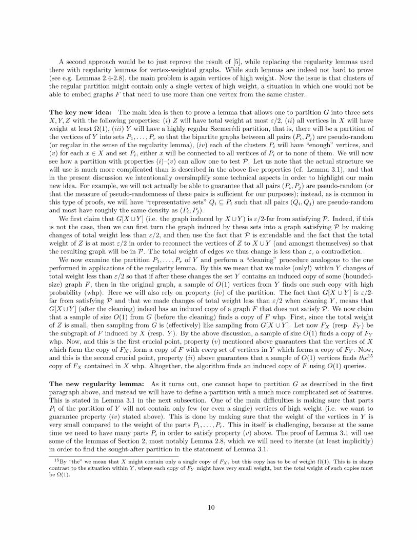
A second approach would be to just reprove the result of [5], while replacing the regularity lemmas usedthere with regularity lemmas for vertex-weighted graphs. While such lemmas are indeed not hard to prove(see e.g. Lemmas 2.4-2.8), the main problem is again vertices of high weight. Now the issue is that clusters ofthe regular partition might contain only a single vertex of high weight, a situation in which one would not beable to embed graphs F that need to use more than one vertex from the same cluster.

The key new idea: The main idea is then to prove a lemma that allows one to partition G into three setsX,Y, Z with the following properties: (i) Z will have total weight at most ε/2, (ii) all vertices in X will haveweight at least Ω(1), (iii) Y will have a highly regular Szemeredi partition, that is, there will be a partition ofthe vertices of Y into sets P1, . . . , Pr so that the bipartite graphs between all pairs (Pi, Pj) are pseudo-random(or regular in the sense of the regularity lemma), (iv) each of the clusters Pi will have “enough” vertices, and(v) for each x ∈ X and set Pi, either x will be connected to all vertices of Pi or to none of them. We will nowsee how a partition with properties (i)–(v) can allow one to test P. Let us note that the actual structure wewill use is much more complicated than is described in the above five properties (cf. Lemma 3.1), and thatin the present discussion we intentionally oversimplify some technical aspects in order to highlight our mainnew idea. For example, we will not actually be able to guarantee that all pairs (Pi, Pj) are pseudo-random (orthat the measure of pseudo-randomness of these pairs is sufficient for our purposes); instead, as is common inthis type of proofs, we will have “representative sets” Qi ⊆ Pi such that all pairs (Qi, Qj) are pseudo-randomand most have roughly the same density as (Pi, Pj).

We first claim that G[X ∪Y ] (i.e. the graph induced by X ∪Y ) is ε/2-far from satisfying P. Indeed, if thisis not the case, then we can first turn the graph induced by these sets into a graph satisfying P by makingchanges of total weight less than ε/2, and then use the fact that P is extendable and the fact that the totalweight of Z is at most ε/2 in order to reconnect the vertices of Z to X ∪ Y (and amongst themselves) so thatthe resulting graph will be in P. The total weight of edges we thus change is less than ε, a contradiction.

We now examine the partition P1, . . . , Pr of Y and perform a “cleaning” procedure analogous to the oneperformed in applications of the regularity lemma. By this we mean that we make (only!) within Y changes oftotal weight less than ε/2 so that if after these changes the set Y contains an induced copy of some (bounded-size) graph F , then in the original graph, a sample of O(1) vertices from Y finds one such copy with highprobability (whp). Here we will also rely on property (iv) of the partition. The fact that G[X ∪ Y ] is ε/2-far from satisfying P and that we made changes of total weight less than ε/2 when cleaning Y , means thatG[X ∪Y ] (after the cleaning) indeed has an induced copy of a graph F that does not satisfy P. We now claimthat a sample of size O(1) from G (before the cleaning) finds a copy of F whp. First, since the total weightof Z is small, then sampling from G is (effectively) like sampling from G[X ∪ Y ]. Let now FX (resp. FY ) bethe subgraph of F induced by X (resp. Y ). By the above discussion, a sample of size O(1) finds a copy of FYwhp. Now, and this is the first crucial point, property (v) mentioned above guarantees that the vertices of Xwhich form the copy of FX , form a copy of F with every set of vertices in Y which forms a copy of FY . Now,and this is the second crucial point, property (ii) above guarantees that a sample of O(1) vertices finds the15

copy of FX contained in X whp. Altogether, the algorithm finds an induced copy of F using O(1) queries.

The new regularity lemma: As it turns out, one cannot hope to partition G as described in the firstparagraph above, and instead we will have to define a partition with a much more complicated set of features.This is stated in Lemma 3.1 in the next subsection. One of the main difficulties is making sure that partsPi of the partition of Y will not contain only few (or even a single) vertices of high weight (i.e. we want toguarantee property (iv) stated above). This is done by making sure that the weight of the vertices in Y isvery small compared to the weight of the parts P1, . . . , Pr. This in itself is challenging, because at the sametime we need to have many parts Pi in order to satisfy property (v) above. The proof of Lemma 3.1 will usesome of the lemmas of Section 2, most notably Lemma 2.8, which we will need to iterate (at least implicitly)in order to find the sought-after partition in the statement of Lemma 3.1.

15By “the” we mean that X might contain only a single copy of FX , but this copy has to be of weight Ω(1). This is in sharpcontrast to the situation within Y , where each copy of FY might have very small weight, but the total weight of such copies mustbe Ω(1).

10

3.2 The Key Lemma

In this subsection we state and prove Lemma 3.1, which is the main ingredient in the proof of the “if” directionof Theorem 1.

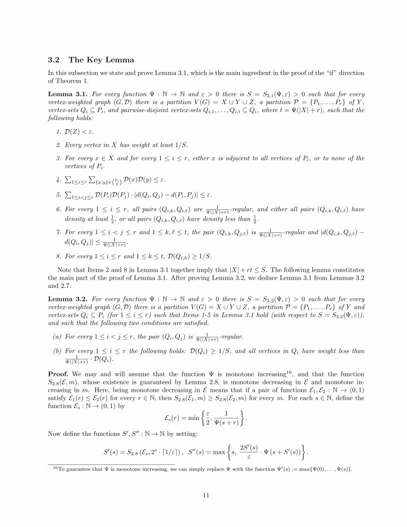
Lemma 3.1. For every function Ψ : N → N and ε > 0 there is S = S3.1(Ψ, ε) > 0 such that for everyvertex-weighted graph (G,D) there is a partition V (G) = X ∪ Y ∪ Z, a partition P = P1, . . . , Pr of Y ,vertex-sets Qi ⊆ Pi, and pairwise-disjoint vertex-sets Qi,1, . . . , Qi,t ⊆ Qi, where t = Ψ(|X|+ r), such that thefollowing holds:

1. D(Z) < ε.

2. Every vertex in X has weight at least 1/S.

3. For every x ∈ X and for every 1 ≤ i ≤ r, either x is adjacent to all vertices of Pi, or to none of thevertices of Pi.

4.∑

1≤i≤r∑x,y∈(Pi2 )D(x)D(y) ≤ ε.

5.∑

1≤i<j≤r D(Pi)D(Pj) · |d(Qi, Qj)− d(Pi, Pj)| ≤ ε.

6. For every 1 ≤ i ≤ r, all pairs (Qi,k, Qi,`) are 1Ψ(|X|+r) -regular, and either all pairs (Qi,k, Qi,`) have

density at least 12 , or all pairs (Qi,k, Qi,`) have density less than 1

2 .

7. For every 1 ≤ i < j ≤ r and 1 ≤ k, ` ≤ t, the pair (Qi,k, Qj,`) is 1Ψ(|X|+r) -regular and |d(Qi,k, Qj,`) −

d(Qi, Qj)| ≤ 1Ψ(|X|+r) .

8. For every 1 ≤ i ≤ r and 1 ≤ k ≤ t, D(Qi,k) ≥ 1/S.

Note that Items 2 and 8 in Lemma 3.1 together imply that |X|+ rt ≤ S. The following lemma constitutesthe main part of the proof of Lemma 3.1. After proving Lemma 3.2, we deduce Lemma 3.1 from Lemmas 3.2and 2.7.

Lemma 3.2. For every function Ψ : N → N and ε > 0 there is S = S3.2(Ψ, ε) > 0 such that for everyvertex-weighted graph (G,D) there is a partition V (G) = X ∪ Y ∪ Z, a partition P = P1, . . . , Pr of Y andvertex-sets Qi ⊆ Pi (for 1 ≤ i ≤ r) such that Items 1-5 in Lemma 3.1 hold (with respect to S = S3.2(Ψ, ε)),and such that the following two conditions are satisfied.

(a) For every 1 ≤ i < j ≤ r, the pair (Qi, Qj) is 1Ψ(|X|+r) -regular.

(b) For every 1 ≤ i ≤ r the following holds: D(Qi) ≥ 1/S, and all vertices in Qi have weight less than1

Ψ(|X|+r) · D(Qi).

Proof. We may and will assume that the function Ψ is monotone increasing16, and that the functionS2.8(E ,m), whose existence is guaranteed by Lemma 2.8, is monotone decreasing in E and monotone in-creasing in m. Here, being monotone decreasing in E means that if a pair of functions E1, E2 : N → (0, 1)satisfy E1(r) ≤ E2(r) for every r ∈ N, then S2.8(E1,m) ≥ S2.8(E2,m) for every m. For each s ∈ N, define thefunction Es : N→ (0, 1) by

Es(r) = min

ε

2,

1

Ψ(s+ r)

.

Now define the functions S′, S′′ : N→ N by setting:

S′(s) = S2.8 (Es, 2s · d1/εe) , S′′(s) = max

s,

2S′(s)

ε·Ψ (s+ S′(s))

.

16To guarantee that Ψ is monotone increasing, we can simply replace Ψ with the function Ψ′(s) := maxΨ(0), . . . ,Ψ(s).

11

Note that S′′(s) ≥ s for every s ∈ N, and that S′ and S′′ are monotone increasing. We define a monotoneincreasing sequence s1, s2, . . . as follows: s1 = 1, and for each i ≥ 2, si = S′′(si−1). We will show that thelemma holds with

S = S3.2(Ψ, ε) = sd2/εe .

Let (G,D) be a vertex-weighted graph. We iteratively define a sequence of pairwise-disjoint vertex-setsX1, X2, . . . ⊆ V (G) as follows: let X1 be the set of all vertices of G of weight at least 1/s1; for each i ≥ 2, let Xi

be the set of all vertices in V (G)\ (X1∪· · ·∪Xi−1) having weight at least 1/si. Since X1, X2, . . . are pairwise-disjoint, there must be 1 ≤ i ≤ d2/εe for which D(Xi) ≤ ε/2. We now set Z ′ = Xi, X = X1 ∪ · · · ∪Xi−1 andY ′ = V (G) \ (X ∪ Z ′) = V (G) \ (X1 ∪ · · · ∪Xi). Note that D(Z ′) ≤ ε/2. Setting s := si−1 ≤ sd2/εe−1 ≤ S,

note that every vertex in X has weight at least 1s (so in particular |X| ≤ s), while every vertex in Y ′ has

weight less than 1si

= 1S′′(s) .

If D(Y ′) < ε2 then D(Y ′ ∪Z ′) < ε, so the assertion of the lemma holds for Y = ∅ and Z = Z ′ ∪ Y ′, and we

are done. So we may and will assume from now on that D(Y ′) ≥ ε2 . Let P ′0 be a partition of Y ′ into d1/εe

parts such that∑P∈P′

0

∑x,y∈(P2)D(x)D(y) ≤ ε, as guaranteed by Lemma 2.1. For every x ∈ X, consider

the partition Px := NY ′(x), Y ′ \NY ′(x) of Y ′. Let P0 be the common refinement of the partitions P ′0 and(Px)x∈X . Then for every x ∈ X and P ∈ P0, either x is adjacent to every vertex of P , or x is not adjacent toany vertex of P . Moreover, we have |P0| ≤ 2|X| · d1/εe ≤ 2s · d1/εe.

Now apply Lemma 2.8 to (G[Y ′],DY ′) with parameters Es and m = 2s · d1/εe, and with the partitionP0 (noting that |P0| ≤ m), to obtain a partition P = P0, P1, . . . , Pr of Y ′ and vertex-sets Qi ⊆ Pi (for1 ≤ i ≤ r), with the properties stated in that lemma. Note that in particular we have

r ≤ S2.8 (Es, 2s · d1/εe) = S′(s). (1)

Set Z = Z ′ ∪ P0 and Y = Y ′ \ P0, noting that D(P0) < Es(0) ≤ ε2 , and hence D(Z) = D(Z ′) + D(P0) < ε,

as required by Item 1 in Lemma 3.1. Items 3 and 4 in Lemma 3.1 hold because each of the sets P1, . . . , Pr iscontained in some part of P0, and hence also in some part of P ′0. Item 2 of Lemma 3.1 was already verifiedabove, and Item 5 of Lemma 3.1 is guaranteed by Lemma 2.8. Item (a) holds because Lemma 2.8 guaranteesthat all pairs (Qi, Qj) are Es(r)-regular, and because Es(r) ≤ 1

Ψ(s+r) ≤1

Ψ(|X|+r) (here we used our choice of Es,the fact that |X| ≤ s, and the monotonicity of Ψ). It remains to prove Item (b). For each 1 ≤ i ≤ r, we have

D(Qi) = DY ′(Qi) · D(Y ′) ≥ DY ′(Qi) ·ε

2≥ ε

2S2.8 (Es, 2s · d1/εe)

=ε

2S′(s)≥ 1

S′′(s)≥ 1

S′′(sd2/εe−1)=

1

sd2/εe=

1

S,

(2)

where in the second inequality we used the guarantees of Lemma 2.8, and later we used our choice of S′ andS′′, the monotonicity of S′′, and the fact that s ≤ sd2/εe−1. Next, fix 1 ≤ i ≤ r and recall that all vertices inQi ⊆ Y ⊆ Y ′ have weight less than

1

S′′(s)≤ 1

Ψ (s+ S′(s))· ε

2S′(s)

≤ 1

Ψ(s+ r)· D(Qi) ≤

1

Ψ(|X|+ r)· D(Qi),

where in the first inequality we used our choice of S′′, in the last two inequalities we used the monotonicityof Ψ, and in the second inequality we also used (1) and an intermediate step in (2). This shows that D(u) <

1Ψ(|X|+r) · D(Qi) for every 1 ≤ i ≤ r and u ∈ Qi, as required.

Proof of Lemma 3.1. Define the functions

ζ : N→ (0, 1), ζ(m) = ζ2.7

(Ψ(m),

1

Ψ(m)

),

and

Ψ′ : N→ N, Ψ′(m) =2Ψ(m)

ζ(m).

12

We may and will assume that the function ζ2.7(t, δ) is monotone decreasing in t and monotone increasing in δ.This assumption implies that the function ζ defined above is monotone decreasing. We prove the lemma with

S = S3.1(Ψ, ε) :=S3.2(Ψ′, ε)

ζ(S3.2(Ψ′, ε))≥ S3.2(Ψ′, ε) .

Let (G,D) be a vertex-weighted graph. Apply Lemma 3.2 to (G,D) with parameters Ψ′ and ε, to obtaina partition V (G) = X ∪ Y ∪ Z, a partition P = P1, . . . , Pr of Y , and subsets Qi ⊆ Pi (for 1 ≤ i ≤ r) suchthat Items 1-5 of Lemma 3.1 hold (with respect to S3.2(Ψ′, ε)), and so do Items (a) and (b) of Lemma 3.2.

Let us now prove that Items 6-8 (in Lemma 3.1) hold. It will be convenient to put m := |X|+ r. By Item(b) in Lemma 3.2 and by our choice of Ψ′, we have

D(u) <1

Ψ′(m)· D(Qi) <

ζ(m)

Ψ(m)· D(Qi) ≤ ζ(m) · D(Qi) (3)

for every 1 ≤ i ≤ r and u ∈ Qi. Recalling our choice of ζ, we see that Lemma 2.7 is applicable to (G[Qi],DQi)with parameters t = Ψ(m) = Ψ(|X|+ r) and δ = 1

Ψ(m) = 1Ψ(|X|+r) . Applying Lemma 2.7 with this input, we

obtain pairwise-disjoint vertex-sets Qi,1, . . . , Qi,t ⊆ Qi satisfying the properties stated in that lemma. Theguarantees of Lemma 2.7 immediately establish Item 6, and also imply that for every 1 ≤ k ≤ t we have

D(Qi,k) ≥ ζ(m) · D(Qi) = ζ(|X|+ r) · D(Qi) ≥ ζ(|X|+ r) · 1

S3.2(Ψ′, ε)≥ ζ(S3.2(Ψ′, ε))

S3.2(Ψ′, ε)=

1

S,

where in the second and third inequalities we used the fact that |X| + r, 1D(Qi)

≤ S3.2(Ψ′, ε), as guaranteed

by Item 2 of Lemma 3.1 and Item (b) of Lemma 3.2; in the third inequality we also used the monotonicityof ζ. This establishes Item 8. It remains to prove Item 7. By Item (a) of Lemma 3.2, the pair (Qi, Qj)

is 1Ψ′(m) -regular for every 1 ≤ i < j ≤ r. Fix any 1 ≤ k, ` ≤ t. Recalling that 1

Ψ′(m) = ζ(m)2Ψ(m) and that

D(Qi,k) ≥ ζ(m) · D(Qi), D(Qj,`) ≥ ζ(m) · D(Qj), we apply Item 1 of Lemma 2.3 to Qi, Qj , Qi,k, Qj,` withparameter α = ζ(m), to conclude that |d(Qi,k, Qj,`) − d(Qi, Qj)| ≤ 1

Ψ′(m) ≤1

Ψ(m) = 1Ψ(|X|+r) , and that the

pair (Qi,k, Qj,`) is 1Ψ(|X|+r) -regular, as required.

3.3 Proof of the Main Result

In this subsection we prove (the “if” direction of) Theorem 1. For a hereditary and extendable graph propertyP, our tester for P will work as follows: given an input (G,D) and a proximity parameter ε, the tester samplesa sequence of vertices u1, . . . , us ∈ V (G) independently and with distribution D, where s = sP(ε) is as inTheorem 4; the tester then accepts if and only if G[u1, . . . , us] satisfies P. Since P is hereditary, this testeraccepts with probability 1 if the input graph satisfies P. In the other direction, Theorem 4 immediately impliesthat if the input (G,D) is ε-far from P then the tester rejects with probability at least 2

3 . So we see that the“if” direction of Theorem 1 follows from Theorem 4.

From now on our goal is to prove Theorem 4. We start by introducing variants of some definitions from[5]. An embedding scheme is a complete graph K with a vertex partition AK ∪BK , such that every vertex inBK is colored black or white, every edge with an endpoint in AK is colored black or white, and every edgecontained in B is colored black, white or grey. Note that one of Ak, Bk may be empty; that the vertices of AKare not colored; and that the edges with at least one endpoint in AK cannot be colored grey. An embeddingfrom a graph F to an embedding scheme K is a map ϕ : V (F )→ V (K) such that the following holds:

1. For every a ∈ AK we have |ϕ−1(a)| ≤ 1.

2. For every b ∈ BK , if b is colored black then ϕ−1(b) induces a complete graph, and if b is colored whitethen ϕ−1(b) induces an empty graph.

3. For every x, y ∈(V (K)

2

), if x, y is colored black then the bipartite graph between ϕ−1(x) and ϕ−1(y)

is complete, and if x, y is colored white then the bipartite graph between ϕ−1(x) and ϕ−1(y) is empty(note that there are no restrictions in the case that x, y is colored grey).

13

Note that Condition 3 implies that for every a ∈ AK and x ∈ V (K) \ a, the bipartite graph between ϕ−1(a)and ϕ−1(x) is either complete or empty. We use the notation F → K to mean that there is an embeddingfrom F to K. For a graph-family F and an integer m, let Fm be the family of all embedding schemes K onat most m vertices, such that there is an embedding from some F ∈ F to K. We now introduce a variant ofthe function ΨF defined in [5].

Definition 3.3. For a graph-family F and an integer m for which Fm 6= ∅, define

ΨF (m) = maxK∈Fm

minF∈F :F→K

|V (F )|.

If Fm = ∅ then define ΨF (m) = 0.

We are now ready to prove Theorem 4 (and thus also the “if” direction of Theorem 1).

Proof of Theorem 4. Let P be a hereditary and extendable graph property. Let F = F(P) be the familyof graphs which do not satisfy P. Fix ε ∈ (0, 1), and let Ψ : N→ N be the function

Ψ(m) = max

8

ε,ΨF (m),

1

δ2.4(ΨF (m), ε8 )

,

where ΨF is defined in Definition 3.3. We may and will assume that the function δ2.4(h, η) is monotonedecreasing in h and monotone increasing in η. Set S := S3.1(Ψ, ε4 ). We prove the theorem with

s = sP(ε) :=2SS+1

δ2.4(S, ε8

) . (4)

Let (G,D) be a vertex-weighted graph which is ε-far from P. Apply Lemma 3.1 to (G,D) with parameterε4 and with Ψ as above, to obtain a partition V (G) = X∪Y ∪Z, a partition P1, . . . , Pr of Y , subsets Qi ⊆ Pi(for 1 ≤ i ≤ r), and pairwise-disjoint subsets Qi,1, . . . , Qi,t ⊆ Qi, such that t = Ψ(|X| + r) and Items 1-8 inLemma 3.1 hold.

We claim that G is 3ε4 -far from any graph G′ on V (G) which satisfies G′[X ∪ Y ] ∈ P. So suppose by

contradiction that there is a graph G′ on V (G) such that G′[X ∪Y ] satisfies P and such that G′ is 3ε4 -close to

G. Since P is extendable, there is a graph G′′ on V (G) = V (G′) such that G′′[X∪Y ] = G′[X∪Y ] and such thatG′′ satisfies P. In order to turn G′ into G′′, we only need to add/delete edges which are incident to vertices ofZ. Therefore, the total weight of edge-changes needed to turn G′ into G′′ is at most D(Z) < ε

4 , as guaranteedby Item 1 of Lemma 3.1. So we see that G can be turned into G′′, which satisfies P, by adding/deleting edgeswhose total weight is less than 3ε

4 + ε4 = ε, in contradiction the assumption that (G,D) is ε-far from P.

We thus proved that G is 3ε4 -far from any graph G′ satisfying G′[X ∪ Y ] ∈ P. Now, let G′ be the graph

obtained from G by doing the following changes:

1. For every 1 ≤ i ≤ r, if d(Qi,k, Qi,`) ≥ 12 for every 1 ≤ k < ` ≤ t then turn Pi into a clique, and if

d(Qi,k, Qi,`) <12 for every 1 ≤ k < ` ≤ t, then turn Pi into an independent set. By Item 6 in Lemma

3.1, one of these options has to hold. The total weight of edge-changes needed in this item is at most ε4

by Item 4 of Lemma 3.1.

2. For every 1 ≤ i < j ≤ r, if d(Qi, Qj) > 1− ε4 then add all edges between Pi and Pj , and if d(Qi, Qj) <

ε4

then remove all edges between Pi and Pj (note that if ε4 ≤ d(Qi, Qj) ≤ 1− ε

4 then no changes are madein the bipartite graph between Pi and Pj). The total weight of edge-changes needed in this item is lessthan ε

2 by Item 5 of Lemma 3.1. Indeed, observe that the total weight of changes between Pi, Pj is lessthan D(Pi)D(Pj) ·

(|d(Qi, Qj)− d(Pi, Pj)|+ ε

4

)by the triangle inequality. Hence, the total weight of

changes is less than ∑1≤i<j≤r

D(Pi)D(Pj) ·(|d(Qi, Qj)− d(Pi, Pj)|+

ε

4

)≤

ε

4+

∑1≤i<j≤r

D(Pi)D(Pj) · |d(Qi, Qj)− d(Pi, Pj)| ≤ε

2.

14

Note that no edge with an endpoint in X was added/deleted in Items 1-2, so G′ and G agree on all edges thatare incident to vertices of X.

We see that the total weight of edge-changes made in Items 1-2 is less than 3ε4 . So G′[X ∪Y ] cannot satisfy

P, implying that G′[X ∪Y ] ∈ F . Note that by definition (see Items 1-2 above), the graph G′ has the followingproperties:

(a) For every 1 ≤ i ≤ r, Pi is either a clique or an independent set in G′. Moreover, Pi is a clique in G′ thendG(Qi,k, Qi,`) ≥ 1

2 for every 1 ≤ k < ` ≤ t, and if Pi is an independent set in G′ then dG(Qi,k, Qi,`) <12

for every 1 ≤ k < ` ≤ t.

(b) For every pair 1 ≤ i < j ≤ r, if there is an edge in G′ between Pi and Pj then dG(Qi, Qj) ≥ ε4 . Then by

Item 7 of Lemma 3.1 we have that dG(Qi,k, Qj,`) ≥ ε4 −

1Ψ(|X|+r) ≥

ε8 for every 1 ≤ k, ` ≤ t. Analogously,

if there is a non-edge in G′ between Pi and Pj then dG(Qi, Qj) ≤ 1 − ε4 , which implies (by Item 7 of

Lemma 3.1) that dG(Qi,k, Qj,`) ≤ 1− ε4 + 1

Ψ(|X|+r) ≤ 1− ε8 for every 1 ≤ k, ` ≤ t.

Now let K be the following embedding scheme: AK = X and BK = b1, . . . , br; for each 1 ≤ i ≤ r, vertexbi is colored black if Pi is a clique in G′ and white if Pi is an independent set in G′; for each x, x′ ∈ X, edgex, x′ is colored black if x, x′ ∈ E(G) and white if x, x′ /∈ E(G); for each x ∈ X, 1 ≤ i ≤ r, edge x, biis colored black if the bipartite graph between x and Pi is complete and white if this bipartite graph is empty(Item 3 in Lemma 3.1 implies that one of these options must hold); finally, for every 1 ≤ i < j ≤ r, edgebi, bj is colored black if the bipartite graph between Pi and Pj is complete in G′, white if the bipartite graphbetween Pi and Pj is empty in G′, and grey otherwise.

Observe that the map ϕ : X ∪ Y → V (K) which maps x to itself (for every x ∈ X = AK) and Pi to bi(for every 1 ≤ i ≤ r), is an embedding from G′[X ∪ Y ] to K. Since |V (K)| = |X| + r, we have K ∈ Fm form := |X|+ r. By the definition of the function ΨF (see Definition 3.3), there is F ∈ F such that F → K and|V (F )| ≤ ΨF (m) = ΨF (|X|+ r) ≤ Ψ(|X|+ r) = t.

Now, fixing an embedding ρ from F to K, write Wi := ρ−1(bi) = wi,1, . . . , wi,fi for 1 ≤ i ≤ r. PutW = W1 ∪ · · · ∪Wr and H = F [W ]. We claim that the sets (Qi,k)1≤i≤r,1≤k≤fi satisfy the requirements 1-2 inLemma 2.4 with respect to h = |V (F )| ≤ ΨF (m), η = ε

8 and H as above, in the graph G. In other words, weshow that one can apply Lemma 2.4 with the sets U1, . . . , Uh being (Qi,k)1≤i≤r,1≤k≤fi , and with G as the hostgraph. We actually already proved that Item 1 in Lemma 2.4 holds; indeed, this follows from the fact thatF → K, the definition of the embedding scheme K, and Items (a)-(b) above. Item 2 of Lemma 2.4 follows fromItems 6-7 of Lemma 3.1, which together imply that for every 1 ≤ i ≤ j ≤ r and 1 ≤ k ≤ fi, 1 ≤ ` ≤ fj (withthe exception of (i, k) = (j, `)), the pair (Qi,k, Qj,`) is δ-regular with δ = 1

Ψ(m) ≤ δ2.4(ΨF (m), ε8 ) ≤ δ2.4(h, ε8 ),

as required.

We thus showed that Lemma 2.4 is applicable to the tuple of sets (Qi,k)1≤i≤r,1≤k≤fi and the graph H =F [W ] (with the parameters defined above). Let U be the set of all tuples (ui,k)1≤i≤r,1≤k≤fi , where ui,k ∈ Qi,k,which induce (in G) a copy of H = F [W ] in which ui,k plays the role of wi,k for every 1 ≤ i ≤ r and 1 ≤ k ≤ fi.By Lemma 2.4, we have

∑(ui,k)i,k∈U

r∏i=1

fi∏k=1

D(ui,k) ≥ δ2.4(h,ε

8

)·r∏i=1

fi∏k=1

D(Ui,k) ≥ δ2.4(

ΨF (m),ε

8

)· S−|W |, (5)

where in the last inequality we used the guarantees of Item 8 in Lemma 3.1 and the monotonicity ofthe function δ2.4. Observe that for every (ui,k)i,k ∈ U , the subgraph of G induced by the vertex-setX ∪ ui,k : 1 ≤ i ≤ r, 1 ≤ k ≤ fi contains an induced copy of F . Indeed, this follows from the definition ofU , the fact that F → K, and the definition of the embedding scheme K. Now sample an (|X|+ |W |)-tuple ofvertices from G according to the distribution D and independently. Note that if every vertex in X appears inthe first |X| vertices of the sample, and if the tuple of the last |W | vertices of the sample belongs to U , thenthe subgraph induced by the sample contains an induced copy of F and hence does not satisfy P (as F ∈ F).The probability for this event is at least

δ2.4

(ΨF (m),

ε

8

)· S−|X|−|W | .

15

Here we used (5) and Item 2 in Lemma 3.1. Next, note that |X| + |W | ≤ |X| + rt ≤ S, where in the lastinequality we used Items 2 and 8 of Lemma 3.1. Similarly, ΨF (m) ≤ t ≤ S. So we see that a sample of Srandom vertices induces a graph which does not satisfy P with probability at least δ2.4

(S, ε8

)·S−S . Therefore,

a sample of s = sP(ε) vertices (see (4)) induces a graph not satisfying P with probability at least

1−(

1− δ2.4(S,ε

8

)· S−S

)s/S= 1−

(1− δ2.4

(S,ε

8

)· S−S

) 2SS

δ2.4(S, ε8 ) ≥ 1− e−2 ≥ 2

3,

as required. This completes the proof.

It is natural to ask about the dependence on ε of the sample complexity of the tester supplied by Theorem 1.One answer is that one cannot prove any upper bound on the sample complexity which holds uniformly forall properties P, because it was shown in [6] that no such bound exists even in the standard model. Supposethen that one is interested only in “simple” properties such as induced H-freeness (for some fixed H). In thiscase, it is not too hard to see that although we are iterating Lemma 2.8, which has wowzer-type (that is,iterated-tower) bounds17 in this setting even for unweighted graphs (see [12, 25]), we are still getting “only”a wowzer-type bound. We should also point out that it might be possible to use the ideas in [12], togetherwith those presented here, in order to get tower-type bounds on the sample complexity of testing inducedH-freeness in the VDF model.

4 VDF-Testable Properties are Extendable and Hereditary

In this section we prove the “only if” direction of Theorem 1. The proof is divided between Propositions 4.1and 4.2. As shown in [19], we can (and will) always assume that a VDF tester only queries the input graphon pairs of vertices which it has sampled.

Proposition 4.1. If a graph property P is not extendable, then P is not testable in the VDF model.

Proof. Since P is not extendable, there is a graph G1 ∈ P, such that no (|V (G1)|+1)-vertex graph satisfyingP contains G1 as an induced subgraph. Let G2 be a graph obtained from G1 by adding a “new” vertex v (andputting an arbitrary bipartite graph between v and V (G1)), let D1 be the uniform distribution on V (G1), andlet D2 be the distribution on V (G2) which assigns weight 1

|V (G1)| to each u ∈ V (G1) ⊆ V (G2) and weight18 0to v.

It is clear that for every integer q, a sample of q vertices from G1 according to D1 is indistinguishable froma sample of q vertices from G2 according to D2. Observe that G1 satisfies P while (G2,D2) is 1

|V (G1)|2 -far

from P. To see that the latter statement is true, observe that by our choice of G1, no matter how we changethe bipartite graph between v and V (G1), we will always get a graph that does not satisfy P. Hence, in orderto make G2 satisfy P, one must change the adjacency relation between a pair of vertices from V (G1), whoseweight (under D2) is 1

|V (G1)| .

Now, the fact that (G1,D1) and (G2,D2) are indistinguishable implies that P is not testable19 in theVDF model.

17To be precise, we mean here that the “standard” way of establishing Lemma 2.8 (which is also the way we prove this lemmain this paper) is via the strong regularity lemma (see Lemma 2.6), which is known to only give wowzer-type bounds [12, 25].In [12], (an unweighted variant of) Lemma 2.8 was proved without the use of the strong regularity lemma, thus giving better,tower-type, bounds. This is alluded to in the following sentence.

18Evidently, if one does not wish to allow vertices of weight 0, then one can instead assign to v a weight tending to 0; or, moreaccurately, a weight that is small enough with respect to (the inverse of) the sample complexity of an alleged tester for P (in aproof by contradiction that such a tester does not exist).

19We note that if P is non-extendable but hereditary, then one can easily obtain infinitely many examples showing that P isnot testable (rather than just the one example given in the proof of Proposition 4.1). Indeed, instead of adding just one vertexto G1, one can add to G1 any number k of vertices (for a large k), and give these new vertices weight o(1/k), while distributingthe remaining weight uniformly among the vertices of G1 (note that such an assignment is precisely what the setting of Theorem

9 forbids). The assumption that P is hereditary implies that every graph obtained in this way is1−o(1)

|V (G1)|2-far from satisfying P.

Also, if the weight given to the “new” vertices is small enough, then these two weighted graphs are indistinguishable by a sampleof any prescribed size.

16

Proposition 4.2. If a graph property P is not hereditary, then P is not testable in the VDF model.

Proof. Since P is not hereditary, there is a graph G1 and an induced subgraph G2 of G1, such that G1

satisfies P but G2 does not. Let D2 be the uniform distribution on V (G2), and let D1 be the distribution onV (G1) which is supported on V (G2) ⊆ V (G1) and uniform when conditioned on V (G2), i.e. D1(u) = 1

|V (G2)|if u ∈ V (G2) and D1(u) = 0 if u ∈ V (G1) \ V (G2). Clearly, for every integer q, a sample of q vertices from G1

according to D1 is indistinguishable from a sample of q vertices from G2 according to D2. Also, G1 satisfiesP, whereas (G2,D2) is 1

|V (G2)|2 -far from P because G2 /∈ P. Thus, P is not testable20 in the VDF model.

5 On Variations of the VDF Model and Related Problems

In the following two subsections we prove Theorems 6, 7, 8 and 9. We then consider two additional problemsrelated to the VDF model; one problem asks if the query complexity in the VDF model is the same as in thestandard model (for P that are testable in the VDF model), and the other asks for a characterization of theproperties that are testable in variants of the VDF model (as in Theorems 6-9). We start by giving the precisedefinitions of the settings considered in Theorems 6-9.

The “large inputs” model In this model, a property P is testable if there exists a function MP : (0, 1)→ Nsuch that for every ε > 0, P is ε-testable with sample complexity depending only on ε under the promise thatinputs (G,D) always satisfy |V (G)| ≥MP(ε).

The “size-aware” model In this model, testers are allowed to receive, as part of the input, the number ofvertices of the input graph.

The “no heavy-weights” (NHW) model In this model, a property P is testable if there exists a functioncP : (0, 1) → (0, 1) such that for every ε > 0, P is ε-testable with sample complexity depending only on εunder the promise that inputs (G,D) always satisfy maxv∈V (G)D(v) ≤ cP(ε).

The “no light-weights” (NLW) model In this model, a property P is testable if for all ε, δ > 0, P isε-testable with sample complexity depending only on ε and δ under the promise that inputs (G,D) alwayssatisfy minv∈V (G)D(v) ≥ δ/|V (G)|.

Theorem 6 (resp. 7, 8, 9) then states that every hereditary property is testable in the “large inputs” (resp.“size-aware”, NHW, NLW) model21.

5.1 Proof of Theorems 6, 7 and 9

In this subsection we prove Theorems 6, 7 and 9, i.e. we show that every hereditary property is testable (withone-sided error) in the “large inputs”, “size-aware” and NLW models. Let us introduce some definitions thatwe will use throughout this subsection. Let P be a hereditary graph property. A graph F is called P-goodif for every r ≥ |V (F )| there is an r-vertex graph which satisfies P and contains F as an induced subgraph;this in particular implies that F itself satisfies P. If F is not P-good then it is called P-bad, and we denoteby rP(F ) the minimal r ≥ |V (F )| such that there is no r-vertex graph which satisfies P and contains F as an

20In analogy to Footnote 19, we note that if P is non-hereditary but extendable then one can obtain infinitely many examplesshowing that P is not testable (rather than just the one given in the proof of Proposition 4.2). Indeed, the extendability of Pimplies that there are arbitrarily large graphs which satisfy P and contain G1 (and hence also G2) as an induced subgraph. Each ofthese graphs (together with an appropriate distribution, as in the proof of Proposition 4.2) is a witness to the non-testability of P.

21Note that if P is testable in the “large inputs” model then it is also testable in the NHW model, because by settingcP (ε) := 1/MP (ε) we can make sure that the input graph has at least MP (ε) vertices. Still, we decided to include a separateproof for Theorem 8 (instead of deducing it from Theorem 6) for two reasons: one is that in the course of the proof we resolveanother open question raised in [19]; and the other is that our proof of Theorem 8 shows that P is testable (in the NHW model)by a tester that accepts if and only if the subgraph induced by the sample satisfies P, whereas the tester given by the proof ofTheorem 6 is not always of this form.

17

induced subgraph. In particular, if F does not satisfy P then it is P-bad and rP(F ) = |V (F )|. Note that sinceP is hereditary, if F is P-bad then there is no graph on r vertices for any r ≥ rP(F ) which satisfies P andcontains F as an induced subgraph. Now let H = H(P) be the property of being P-good. Then H ⊆ P andH is hereditary, which follows from the definition of P-goodness and the fact that P is hereditary. Observemoreover that H is extendable. Indeed, let G ∈ H, and suppose, for the sake of contradiction, that for everyG′ on |V (G)| + 1 vertices which contains G as an induced subgraph, it holds that G′ /∈ H. Then for everysuch G′, there is no graph on rP(G′) vertices that satisfies P and contains G′ as an induced subgraph. Butthis means that there is no graph on maxG′ rP(G′) vertices which satisfies P and contains G as an inducedsubgraph, in contradiction to G ∈ H. We note also that if P itself is extendable then H = P.

For an integer s ≥ 1, let RP(s) be the maximum of rP(F ) over all P-bad graphs F with at most s vertices;if no such graphs exist, we set RP(s) = 0 (this will not matter later on). We are now ready to prove Theorem6, which we rephrase as follows.

Proposition 5.1. For every hereditary property P there are functions MP , sP : (0, 1)→ N such that for everyε > 0, the property P is ε-testable with one-sided error and sample complexity sP(ε) under the promise thatinputs (G,D) always satisfy |V (G)| ≥MP(ε).

Proof. Consider the (extendable and hereditary) property H = H(P) defined above. By Theorem 4, thereis a function sH : (0, 1) → N such that for every ε > 0 and for every vertex-weighted graph (G,D) which isε-far from H, a sample of s vertices from G (taken from D) induces a subgraph which does not satisfy H withprobability at least 2

3 .

Our (“large inputs”-model) tester for P samples sH(ε) vertices, and accepts if and only if the subgraphinduced by the sample satisfies H. We prove the proposition with M = MP(ε) := RP(sH(ε)).

Let (G,D) be a vertex-weighted graph with |V (G)| ≥ M . Suppose first that G satisfies P. Our goal is toshow that the subgraph induced by a sample of sH(ε) vertices, taken from D and independently, satisfiesH withprobability 1. So suppose by contradiction that G contains an induced subgraph F on at most sH(ε) verticeswhich does not satisfy H. In other words, F is P-bad. By the definition of rP(F ), there is no graph on rP(F )vertices which satisfies P and contains F as an induced subgraph. As |V (G)| ≥ M = RP(sH(ε)) ≥ rP(F ),and as P is hereditary, we get that G does not satisfy P, a contradiction.

Suppose now that (G,D) is ε-far from P. Then (G,D) is also ε-far from H, as H ⊆ P. By our choice ofsH(ε), a sample of sH(ε) vertices of G, taken from D and independently, does not satisfy H with probabilityat least 2

3 . So our tester rejects (G,D) with probability at least 23 , as required.

It is natural to ask whether we can replace the function MP(ε) in Lemma 5.1 by a constant dependingonly on P (and not on ε). As is shown in the following proposition, we cannot.

Proposition 5.2. There is a hereditary property P such that for every M > 0, there is no tester for P in theVDF model even if we are guaranteed that the input graph has at least M vertices.

Proof. For each k ≥ 3, let C∗k be the graph obtained from the k-cycle Ck by adding an isolated vertex.Consider the property P = C∗k : k ≥ 3-freeness. Let M > 0. Set G = CM and G′ = C∗M . Let D be theuniform distribution on V (G), and let D′ be the distribution on V (G′) which assigns weight 0 to the isolatedvertex in G′, and is uniform on the rest of the vertices of G′. Then G ∈ P and (G′,D′) is 1

M2 -far from P,but a sample (of any number of vertices) from (G,D) is indistinguishable from a sample of the same size from(G′,D′). This shows that P is not testable even if we require input graphs to have at least M vertices.

We now move on to prove Theorem 7.

Proof of Theorem 7. Let P be a hereditary graph property. Our goal is to design (and prove the correctnessof) a one-sided-error tester for P in the VDF model, provided that the tester receives |V (G)| as part of theinput. Let MP : (0, 1)→ N be as in Lemma 5.1. On input ε ∈ (0, 1), G and D (where G is a graph and D isa distribution on V (G)), our tester works as follows:

1. If |V (G)| ≥ MP(ε), then invoke the tester whose existence is guaranteed by Lemma 5.1, and accept ifand only if this tester accepts.

18

2. Otherwise, i.e. if |V (G)| < MP(ε), then do the following: setting M := MP(ε) and t := M log(3M)/ε,sample vertices u1, . . . , ut ∈ V (G) according to D and independently, and put U := u1, . . . , ut. Acceptif and only if there exists a graph on |V (G)| vertices which satisfies P and contains G[U ] as an inducedsubgraph (in the notation introduced at the beginning of this subsection, this is the same as saying thatrP(G[U ]) > |V (G)|).

Let us prove the correctness of our tester. First, Lemma 5.1 guarantees that if |V (G)| ≥ MP(ε) then thetester works correctly; namely, it accepts with probability 1 if G ∈ P, and rejects with probability at least 2

3if (G,D) is ε-far from P.

So from now on we may assume that |V (G)| < MP(ε). Suppose first that G ∈ P. Evidently, for everyU ⊆ V (G) there is a graph on |V (G)| vertices which satisfies P and contains G[U ] as an induced subgraph(indeed, G is such a graph). Hence, the tester accepts G with probability 1 (see Item 2).

Now suppose that (G,D) is ε-far from P. Observe that for each v ∈ V (G), the probability that v /∈ U is

(1−D(v))t ≤ e−D(v)·t =

(1

3M

)−D(v)·M/ε

.

By taking the union bound over all (at most |V (G)| < m) vertices v ∈ V (G) which satisfy D(v) ≥ ε/M , we seethat the probability that there is v ∈ V (G)\U with D(v) ≥ ε/M , is at most 1

3 . Suppose that every v ∈ V (G)\Usatisfies D(v) < ε/M (this happens with probability at least 2

3 ). Then D(V (G)\U) < |V (G)| ·ε/M < ε (wherein the last inequality we used our assumption that |V (G)| < M). Now, if (by contradiction) there is a graphG′ on |V (G)| vertices which satisfies P and contains G[U ] as an induced subgraph, then one can turn G intoG′ by only adding/deleting edges which are incident to vertices in V (G) \ U . Since D(V (G) \ U) < ε, thisstands in contradiction to the assumption that (G,D) is ε-far from P. We conclude that there is no suchgraph G′. This implies that (G,D) is rejected with probability at least 2

3 , as required.

Finally, we prove Theorem 9, i.e. that every hereditary property is testable in the NLW model. We restatethis theorem as follows.

Proposition 5.3. For every hereditary property P there is a function tP : (0, 1)2 → N such that for allε, δ > 0, the property P is ε-testable with one-sided error and sample complexity tP(ε, δ) under the promisethat inputs (G,D) always satisfy minv∈V (G)D(v) ≥ δ/|V (G)|.

Proof. We start by specifying the function tP(ε, δ). Consider the (extendable and hereditary) propertyH = H(P) defined above. By Theorem 4, there is a function sH : (0, 1) → N such that for every ε > 0 andfor every vertex-weighted graph (G,D) which is ε-far from H, a sample of sH(ε) vertices of G (taken from D)induces a subgraph which does not satisfy H with probability22 at least 5

6 . Now set R := RP(sH(ε)) and

t = tP(ε, δ) := max sH(ε), 2R log(6R)/δ .

Our tester for P in the NLW model simply samples a sequence of tP(ε, δ) vertices of the input and acceptsif and only if the subgraph induced by the sample satisfies P. Evidently, this tester accepts with probability1 if the input satisfies P. So to establish the correctness of our tester, it suffices to show that it rejects withprobability at least 2

3 if the input (G,D) is ε-far from P.

Let ε, δ > 0, and let (G,D) be a vertex-weighted graph on n vertices which is ε-far from P, and in which allvertices have weight at least δ/n. Let u1, . . . , ut be a sequence of t = tP(ε, δ) random vertices of G, sampledaccording to D and independently, and set U = u1, . . . , ut. We need to show that with probability at least23 , G[U ] does not satisfy P. Suppose first that n < 2R. We claim that in this case we have U = V (G) withprobability at least 2

3 (this is clearly sufficient because G itself does not satisfy P). For a vertex v ∈ V (G),the probability that ui 6= v for every 1 ≤ i ≤ t is

(1−D(v))t ≤

(1− δ

n

)t<

(1− δ

2R

)t≤ e− δt

2R ≤ 1

6R.

22The statement of Theorem 4 only guarantees a success probability of 23

, but this can clearly be amplified to 56

by repeatingthe experiment O(1) times.

19

So by the union bound over all n < 2R vertices of G, we see that with probability at least 23 , U = V (G), as

required.

Suppose now that n ≥ 2R. Our choice of s = sH(ε) guarantees that with probability at least 56 , the graph

F := G[u1, . . . , us] does not satisfy H, meaning that it is P-bad. We will now show that with probabilityat least 5

6 , we have |U | ≥ R. This will imply that with probability at least 23 , G[U ] contains as an induced

subgraph a P-bad graph F on at most sH(ε) vertices, and also |U | ≥ R = RP(sH(ε)) ≥ rP(F ). By thedefinition of rP(F ), this would imply that G[U ] does not satisfy P, as required.

So from now on, our goal is to show that |U | ≥ R with probability at least 56 . Fix a partition of V (G) into

R sets V1, . . . , VR, each of size at least b nRc ≥n

2R . For each 1 ≤ i ≤ R, let Ai be the event that U ∩ Vi 6= ∅.Note that if Ai occurs for every 1 ≤ i ≤ R, then |U | ≥ R. Since D(Vi) ≥ |Vi| · δn ≥

n2R ·

δn = δ

2R , the probabilitythat Ai does not occur is at most

(1−D(Vi))t ≤

(1− δ

2R

)t≤ e− δt

2R ≤ 1

6R.

By the union bound, the probability that there is 1 ≤ i ≤ R for which Ai does not occur, is at most 16 , as

required. This completes the proof.

5.2 Proof of Theorem 8

In this subsection we prove Theorem 8, i.e. we show that every hereditary property is testable in the NHWmodel. Again, we rephrase as follows.

Proposition 5.4. For every hereditary property P there are functions tP : (0, 1)→ N and cP : (0, 1)→ (0, 1)such that for every ε > 0, the property P is ε-testable with one-sided error and sample complexity tP(ε) underthe promise that inputs (G,D) always satisfy maxv∈V (G)D(v) ≤ cP(ε).

The key idea in the proof of Proposition 5.4, which appeared in [19], is to “blow up” the vertex-weightedgraph (G,D) by replacing each vertex v with a vertex-set whose size is proportional to D(v), and thus obtainan (unweighted) graph G′, to which one can apply known testability results in the standard model.

Let us introduce some definitions. For a graph G, say on V (G) = v1, . . . , vn, and for integers b1, . . . , bn ≥0, a (b1, . . . , bn)-blowup of G is any graph admitting a vertex-partition V1∪· · ·∪Vn such that |Vi| = bi for every1 ≤ i ≤ n, and such that the bipartite graph between Vi and Vj is complete if vi, vj ∈ E(G) and empty ifvi, vj /∈ E(G). The sets V1, . . . , Vn are called the blowup-sets. Note that we do not pose any restrictions onthe graphs induced by the sets V1, . . . , Vn; these graphs may be arbitrary. For simplicity of presentation, weassume henceforth that all vertex-weights are rational23. Now let D be a distribution on V (G) = v1, . . . , vn,and let N ∈ N be such that D(vi) · N is an integer for every 1 ≤ i ≤ n; such an N is called admissible. A(D, N)-blowup of G is a (b1, . . . , bn)-blowup of G with bi = D(vi) ·N for every 1 ≤ i ≤ n. Note that a blowupis always treated as “unweighted” (in other words, the distribution on its vertices is uniform). Goldreich [19]proved that for every graph F and ε ∈ (0, 1), if a vertex-weighted graph (G,D) is ε-far from being F -free,then for every admissible N , any (D, N)-blowup of G is ε

(|V (F )|2 )

-far from being F -free. Goldreich further asked

whether the(|V (F )|

2

)−1-factor can be avoided. In the following lemma we show that this is indeed the case,

and moreover that an analogous statement holds for every hereditary property. This lemma is also the keyingredient in the proof of Proposition 5.4.

Lemma 5.5. Let P be a hereditary graph property and let (G,D) be a vertex-weighted graph which is ε-farfrom P. Then for every admissible N , any (D, N)-blowup of G is ε-far from P.

23If one allows general (i.e. possibly irrational) weights, then it is necessary to change the definition of a (D, N)-blowup byrounding D(vi) ·N to the closest integer. This results in an additive error of n

Nin the conclusion of Lemma 5.5, due to rounding.

Consequently, in (the proofs of) Propositions 5.4 and 5.7 we need to consider (D, N)-blowups with N →∞ in order to have thiserror term go to 0. We also need to replace ε in several places with (say) ε

2(or any other number smaller than ε). For example,

the conclusion of Proposition 5.7 should be that P is testable in the VDF model by a tester having one-sided error and samplecomplexity qP (ε/2).

20

Proof. Fix any admissible N and let G′ be a (D, N)-blowup of G. As above, we use v1, . . . , vn to denote thevertices of G, and V1, . . . , Vn to denote the corresponding blowup sets. Suppose by contradiction that thereis a graph H ′ on V (G′) that satisfies P and is ε-close to G′. Let H be the random graph defined as follows:the vertex-set of H is V (H) = V (G) = v1, . . . , vn. To define the edge-set of H, sample for each 1 ≤ i ≤ na vertex ui ∈ Vi uniformly at random, and make vi, vj an edge in H if and only if ui, uj is an edge in H ′

(for 1 ≤ i < j ≤ n). Then H satisfies P (with probability 1) because H is isomorphic to an induced subgraphof H ′ and P is hereditary. Let us compute the expected distance between H and G (here the distance is withrespect to the distribution D). For each 1 ≤ i < j ≤ n, the probability that vi, vj ∈ E(G)4E(H) is precisely

|EG′(Vi, Vj)4EH′(Vi, Vj)||Vi||Vj |

=|EG′(Vi, Vj)4EH′(Vi, Vj)|

D(vi)D(vj)N2.

Hence, the expected distance between H and G is∑1≤i<j≤n

D(vi)D(vj) ·|EG′(Vi, Vj)4EH′(Vi, Vj)|

D(vi)D(vj)N2=

1

N2

∑1≤i<j≤n

|EG′(Vi, Vj)4EH′(Vi, Vj)| < ε,

where the last inequality uses the assumption that G′ is ε-close to H ′. So G is ε-close to a graph H whichsatisfies P, a contradiction.

By combining Lemma 5.5 with the result of [5] (that all hereditary properties are testable with one-sidederror in the standard model), we obtain the following: for every hereditary property P, for every vertex-weighted graph (G,D) which is ε-far from P, for every admissible N and for every (D, N)-blowup G′ ofG, it holds that G′ is ε-far from P with respect to the uniform distribution, and hence a sample of somes = sP(ε) vertices of G′, taken uniformly and independently, induces a graph which w.h.p. does not satisfyP. Observe that this induced subgraph of G′ has (essentially) the same distribution as the graph S on [s]obtained by sampling vertices u1, . . . , us ∈ V (G) from D independently, and letting i, j ∈ E(S) if and onlyif ui, uj ∈ E(S) (this is precisely the graph defined in Theorem 5). We thus established Theorem 5, aspromised in Subsection 1.2.

As noted in Subsection 1.2, the graph S defined above is a blowup of an induced subgraph of G, but is notnecessarily a subgraph of G in itself. This is because the sequence u1, . . . , us might contain repeated vertices.In other words, it may be the case that G′ contains “forbidden subgraphs” which use several vertices fromone of the blowup-sets, and thus do not correspond to “forbidden subgraphs” in G. This creates an obstaclefor proving Proposition 5.4, because in order to prove this proposition we need to know that a (suitablychosen) random induced subgraph of G (and not just the blowup thereof) does not satisfy P w.h.p. To avoidthis obstacle, we use the assumption that all vertices in G have relatively small weight, which guaranteesthat it is unlikely to sample more than once from some blowup-set (or in other words, that S is isomorphicto G[u1, . . . , us].). We note that a different way of dealing with this obstacle is to restrict ourselves toproperties for which we can guarantee, by appropriately choosing the graphs inside the blowup-sets, thatthere would not be any minimal forbidden subgraph which uses several vertices from one of the blowup-sets,see Subsection 5.3.

Proof of Proposition 5.4. We start by specifying the functions tP and cP . By the main result of [5], thereis a function qP : (0, 1)→ N such that for every ε > 0 and for every (unweighted) graph G which is ε-far fromP, a sample of qP(ε) vertices from G, taken uniformly at random and independently, induces a graph whichdoes not satisfy P with probability at least 5

6 . Now set tP(ε) := qP(ε) and

cP(ε) :=1

3q2P(ε)

.

Our tester for P in the NHW model simply samples a sequence of t = tP(ε) vertices of the input andaccepts if and only if the subgraph induced by the sample satisfies P. Evidently, this tester accepts with

21

probability 1 if the input satisfies P. So to establish the correctness of our tester, it suffices to show that itrejects with probability at least 2

3 if the input (G,D) is ε-far from P.

Let ε > 0 and let (G,D) be a vertex-weighted graph on n vertices which is ε-far from P, and in whichall vertices have weight at most c, where c = cP(ε). Write V (G) = v1, . . . , vn and fix an admissible N ,that is, a positive integer N such that D(vi) · N is an integer for every 1 ≤ i ≤ n. Let G′ be an arbitrary(D, N)-blowup of G, and denote the blowup-sets by V1, . . . , Vn. By Lemma 5.5, G′ is ε-far from P. Thisimplies that a random sequence u1, . . . , uq of q = qP(ε) vertices of G′, sampled uniformly and independently,induces a graph which does not satisfy P with probability at least 5

6 .

Let ϕ : V (G′) → V (G) be the map which maps all elements of Vi to vi (for every 1 ≤ i ≤ n). Observethat for u ∈ V (G′) sampled uniformly, the random vertex ϕ(u) ∈ V (G) has the distribution D (because|Vi| = D(vi) ·N = D(vi) · |V (G′)|). Furthermore, if a set U ⊆ V (G′) satisfies |Vi ∩U | ≤ 1 for every 1 ≤ i ≤ n,then G[ϕ(U)] is isomorphic to G′[U ]. Let u1, . . . , uq be a random sequence of vertices of G′, sampled uniformlyand independently, and set U := u1, . . . , uq. Recall that G′[U ] does not satisfy P with probability at least56 . Furthermore, the probability that |Vi ∩ U | ≥ 2 for some 1 ≤ i ≤ n is at most

n∑i=1

(q

2

)· D2(vi) ≤

q2

2· c ·

n∑i=1

D(vi) =q2

2· c =

1

6.

We conclude that with probability at least 23 , G′[U ] does not satisfy P and |Vi ∩ U | ≤ 1 for every 1 ≤ i ≤ n,

implying that G[ϕ(U)] does not satisfy P either. This completes the proof.

It is natural to ask whether the function cP(ε) from Proposition 5.4 needs to depend on ε, namely whetherthe statement of Proposition 5.4 holds even if cP is a constant function (depending only on P). The proof ofProposition 5.2 shows, however, that this is not the case. In other words, allowing cP(ε) to depend on ε isunavoidable.

5.3 Testing in the VDF Model vs. Testing in the Standard Model

It is natural to ask about the relation between the sample complexity for testing a property in the VDF modeland the sample complexity for testing it in the standard model. More specifically, it will be interesting toresolve the following:

Problem 5.6. Is it true that every extendable hereditary property P can be tested in the VDF model with thesame (or close to the same) sample complexity as in the (standard) dense graph model?

While at present we cannot answer this question, we can show that many natural properties P can betested in the VDF model with (exactly) the same sample complexity as that of the (optimal) tester for P inthe standard model, which works by sampling a certain number of vertices and accepting if and only if theyinduce a graph which satisfies P. This is explained in the following paragraph.

As mentioned in Subsection 5.2, the assumption made in Proposition 5.4 regarding the non-existence ofhigh-weight vertices is needed in order to handle the possibility of having copies of some (forbidden) graph Fin G′ which do not correspond to copies of F in G (where G′ is some blowup of G). For some graph properties,however, such an assumption is not required, as we can make sure that every copy of a minimal forbiddengraph in G′ will correspond to such a copy in G. To make this precise, we need the following definition. Afamily of graphs F is said to be blowup-avoidable if for every graph G, say on v1, . . . , vn, and for everyn-tuple of integers b1, . . . , bn ≥ 0, there is a (b1, . . . , bn)-blowup G′ of G with blowup-sets V1, . . . , Vn, suchthat there is no induced copy of any F ∈ F in G′ which intersects some Vi in at least 2 vertices; in otherwords, for every F ∈ F , every induced copy of F in G′ corresponds to an induced copy of F in G. We saythat a hereditary property P is blowup-avoidable if the family of minimal forbidden induced subgraphs for Pis blowup-avoidable. We now prove the following proposition, which partially resolves Problem 5.6. The proofis similar to that of Proposition 5.4.

Proposition 5.7. Let P be a hereditary graph property which is blowup-avoidable, and suppose that P admitsa tester in the standard model, which works by sampling qP(ε) vertices uniformly at random and independently,

22

and accepting if and only if the subgraph induced by the sample satisfies P. Then P is testable in the VDFmodel by a tester having one-sided error and sample complexity24 qP(ε).

Proof. Given an input (G,D), the required VDF tester for P samples (from D) a sequence of qP(ε) vertices,and accepts if and only if the subgraph induced by the sample satisfies P. Since P is hereditary, this testeraccepts with probability 1 if the input graph satisfies P. So it remains to show that if the input (G,D) isε-far from P, then with probability at least 2

3 , a sequence of qP(ε) vertices of G, sampled according to D andindependently, induces a graph which does not satisfy P.

Let F = F(P) be the family of minimal forbidden induced subgraphs for P. Let (G,D) be a vertex-weighted graph on n vertices, which is ε-far from P. Write V (G) = v1, . . . , vn and fix an admissible N , thatis, a positive integer N such that D(vi) ·N is an integer for every 1 ≤ i ≤ n. As P is blowup-avoidable, thereis a (D, N)-blowup G′ of G with blowup-sets V1, . . . , Vn, such that there is no induced copy of any F ∈ Fin G′ which intersects some Vi in at least 2 vertices. By Lemma 5.5, G′ is ε-far from P. So by our choiceof qP(ε), with probability at least 2

3 it holds that a sequence of qP(ε) vertices of G′, sampled uniformly andindependently, induces a graph which does not satisfy P, and hence contains an induced copy of some F ∈ F .

Let ϕ : V (G′)→ V (G) be the map which maps all elements of Vi to vi (for every 1 ≤ i ≤ n). Observe thatfor u ∈ V (G′) sampled uniformly, the random vertex ϕ(u) ∈ V (G) has the distribution D. Note that by ourchoice of G′, if u1, . . . , ur ∈ V (G′) span an induced copy of some F ∈ F (in the graph G′), then ϕ|u1,...,ur isinjective (and hence an isomorphism), which implies that ϕ(u1), . . . , ϕ(ur) span an induced copy of F in G. Itis now easy to see that a sequence of qP(ε) vertices of G, sampled from D and independently, does not satisfyP with probability at least 2

3 , as required.

To demonstrate the usefulness of Proposition 5.7, observe that induced F -freeness is blowup-avoidable forevery F ∈ P2, P3, C4 (here Pk is the path with k edges). Indeed, this is established by taking the blowup-sets(in the definition of blowup-avoidability) to be cliques. By combining Proposition 5.7 with known results forthe standard model [5, 3, 16], we immediately get that induced F -freeness is testable in the VDF model withsample complexity poly(1/ε) if F ∈ P2, P3, and with sample complexity at most 2poly(1/ε) if F = C4.

We now describe another corollary of Proposition 5.7. We say that a graph property P is closed underblowups if for every graph G satisfying P, every blowup of G in which the blowup-sets are independent sets alsosatisfies P. We claim that if a hereditary property P is closed under blowups then it is also blowup-avoidable.To see this, let F be the set of minimal forbidden induced subgraphs for P, let G be an n-vertex graph, letb1, . . . , bn ≥ 0 be integers and let G′ be the (b1, . . . , bn)-blowup of G in which the blowup-sets, V1, . . . , Vn, areindependent. Let F ∈ F and suppose that G′ contains an induced copy of F . If, by contradiction, this copyintersects some Vi in more than one vertex, then F is a blowup of some graph F ′ with |V (F ′)| < |V (F )|, wherethe blowup-sets are independent sets. Since P is closed under blowups and F /∈ P, we must have F ′ /∈ P; butthis contradicts the fact that F is a minimal forbidden induced subgraph for P.

So we see that the conclusion of Proposition 5.7 applies to hereditary properties which are closed underblowups. Some examples of such properties include Kt-freeness; the property of having a homomorphism intoa fixed graph H (and in particular the property of being k-colorable); and the property of being the blowupof a fixed graph H (cf. [8]).

On the negative side, there are many natural hereditary properties which are extendable but not blowup-avoidable, such as the property of being H-free for a graph H which is neither a clique nor contains isolatedvertices. It would be interesting to resolve Problem 5.6 for these properties.

5.4 Which Properties are Testable in the Variations of the VDF Model?

It may be interesting to characterize the graph properties which are testable in each of the variations of theVDF model (defined at the beginning of Section 5).

Problem 5.8. Which graph properties are testable in the “large inputs”/“size-aware”/NHW/NLW model?

24Provided that the input distributions are only allowed to assign rational weights. If irrational weights are allowed, then thesample complexity (of the VDF tester for P) should be slightly increased to (say) qP (ε/2), see Footnote 23.

23

While at the moment we are unable to resolve Problem 5.8, we can rule out some initial guesses. A firstguess might be that only hereditary properties are testable in these models. This, however, turns out tobe false; for example, connectivity and hamiltonicity are testable in each of these models, as implied by thefollowing proposition.

Proposition 5.9. Let P be a property such that for every ε > 0 there is M(ε) so that every vertex-weightedgraph on at least M(ε) vertices is ε-close to P. Then P is testable in all four variations of the VDF model.

Proof. The fact that P is testable in the “large inputs” (resp. NHW) model is trivial; indeed, by choosingMP(ε) := M(ε) (resp. cP(ε) := 1/M(ε)) we can make sure that every input graph will be ε-close to P, so atester that simply accepts without making any queries is a valid tester for P.

Let us now consider the NLW model. Given ε, δ > 0 and an input graph (G,D) with all vertex-weights atleast δ

|V (G)| , our tester for P works as follows: setting M := M(ε), the tester samples CM log(M)/δ vertices

according to D and independently (where C is some large constant); if the number of distinct vertices in thesample is at least M then the tester accepts (without making any queries), and otherwise the tester acceptsif and only if the subgraph induced by the sample satisfies P. To see that this is a valid tester, observe thatif G has less than M vertices then w.h.p. the tester samples all the vertices, and if G has at least M verticesthen w.h.p. there are at least M distinct vertices in the sample. This can be argued similarly as in the proofof Proposition 5.3, using that all vertices have weight at least δ

|V (G)| ; we omit the details.

Finally, let us prove that P is testable in the “size-aware” model. On input ε > 0 and (G,D), our tester forP (in the “size-aware” model) does the following: if |V (G)| ≥ M(ε) then the tester accepts without makingany queries, and if |V (G)| < M(ε) then the tester samples t := M log(3M)/ε vertices u1, . . . , ut ∈ V (G)according to the distribution D and independently, where M = M(ε), and accepts if and only if there is agraph on |V (G)| vertices which satisfies P and contains G[u1, . . . , ut] as an induced subgraph. The proof ofcorrectness for this tester is similar to the proof of Theorem 7, and we leave the details to the reader.

In order to apply Proposition 5.9 to the properties of connectivity and hamiltonicity, we observe that anyvertex-weighted graph (G,D) with |V (G)| ≥ 1/ε is ε-close to being hamiltonian (and hence also connected).To see that this holds, take a random (cyclic) ordering v1, . . . , vn of the vertices of G, and observe that forevery pair of distinct u,w ∈ V (G), the probability that there is 1 ≤ i ≤ n such that u,w = vi, vi+1 isn/(n2

)= 2

n−1 . This implies that the expected value of∑ni=1D(vi)D(vi+1) is 2

n−1 ·∑u,w∈V (G)D(u)D(w) =

2n−1 ·

12 ·(

1−∑v∈V (G)D(v)2

)≤ 1

n−1 ·(1− 1

n

)= 1

n , where the last inequality follows from Cauchy-Schwarz

(and the first sum is over unordered pairs u,w). This means that we can create a hamilton cycle by addingedges of total weight at most 1

n ≤ ε. Let us also note that for connectivity there is a simpler argument: if(G,D) is a vertex-weighted graph with |V (G)| ≥ 1/ε, then there is v ∈ V (G) with D(v) ≤ ε, and we can makeG connected by connecting v to all other vertices.

Note that in some of the restricted models (e.g. the NLW model), the tester given by (the proof of)Proposition 5.9 has 2-sided error. It is also not hard to see that the NLW model admits no 1-sided-error testerfor, e.g., connectivity. This shows that (some of) the restricted models allow for properties which are testablewith 2-sided error but not with 1-sided error (unlike the “ordinary” VDF model, where we know that everytestable property can be tested with 1-sided error, as follows from Theorems 1 and 4; see also [19, Theorem 2.3]).

Another natural guess regarding the answer to Problem 5.8 would be that every property which is testablein the standard model is also testable in the restricted models (see [2] for a characterization of the propertiestestable in the standard model). This guess is ruled out by the following proposition, which describes aproperty which is testable in the standard model but not in the restricted models.

Proposition 5.10. The property P of having edge-density25 at most 14 is not testable in either of the four

variants of the VDF model.

Proof. Let G1 be the n-vertex graph consisting of a clique of size n2 and n

2 isolated vertices, and let D1 bethe uniform distribution on V (G1). Let G2 be the n-vertex graph consisting of a clique X of size 3n

4 and n4

25The edge-density of a (possibly vertex-weighted) graph G is defined as 2e(G)/|V (G)|2; in other words, the density is definedwith respect to the uniform distribution on V (G), and not with respect to the given distribution D.

24

isolated vertices, and let D2 be the distribution on V (G2) that assigns weight 23n to every vertex of X, and

weight 2n to every vertex of V (G2)\X. Note that (G1,D1) and (G2,D2) are valid inputs in each of the variants

of the VDF model (provided that n is large enough), and that G1 satisfies P while (G2,D2) is Ω(1)-far fromP. On the other hand, we now show that for every q, a sample of q vertices from (G1,D1) is indistinguishablefrom a sample of q vertices from (G2,D2) (provided that n is large enough with respect to q). To this end,let Ui be a set of q random vertices of Gi sampled according to Di and independently (for i = 1, 2). Thenfor both i = 1, 2, the graph Gi[Ui] consists of a clique and some isolated vertices. Letting Xi be the clique inGi[Ui], we have

P[|X1| = k] = o(1) +

(q

k

)·k−1∏i=0

(n2− i)·q−k−1∏i=0

(n2− i)·(

1

n

)q= (1 + o(1))

(q

k

)·(

1

2

)qand

P[|X2| = k] = o(1) +

(q

k

)·k−1∏i=0

(3n

4− i)·q−k−1∏i=0

(n4− i)·(

2

3n

)k·(

2

n

)q−k= (1 + o(1))

(q

k

)·(

1

2

)q,

where in both cases, the additive term o(1) accounts for the event that some vertex has been sampled morethan once. So we see that |P[|X1| = k]− P[|X2| = k]| = o(1). This implies that the total variation distancebetween the distribution of G1[U1] and the distribution of G2[U2] is o(1). It follows that P is not testable inany of the four variants of the VDF model (note that knowing n does not help to distinguish between (G1,D1)and (G2,D2), since these graphs have the same number of vertices).

The proof of Proposition 5.10 can be adapted to show that other properties are also not testable in eitherof the variants of the VDF model. These properties include the property of having a cut with at least αn2

edges (for 0 < α < 14 ) and the property of containing a clique with at least αn vertices (for 0 < α < 1).

Acknowledgements We are grateful to an anonymous referee for spotting a gap in the proof of Theorem1 in a preliminary version of the paper.

References

[1] N. Alon, E. Fischer, M. Krivelevich and M. Szegedy, Efficient testing of large graphs. Combinatorica 20(2000), 451–476.

[2] N. Alon, E. Fischer, I. Newman and A. Shapira, A combinatorial characterization of the testable graphproperties: it’s all about regularity. SIAM Journal on Computing, 39(1) (2009), 143–167.

[3] N. Alon and J. Fox, Easily testable graph properties, Combin. Probab. Comput. 24 (2015), 646–657.

[4] N. Alon and A. Shapira, A characterization of easily testable induced subgraphs. Combinatorics, Proba-bility and Computing 15 (2006), 791–805.

[5] N. Alon and A. Shapira, A characterization of the (natural) graph properties testable with one-sidederror. SIAM Journal on Computing 37 (2008), 1703–1727.

[6] N. Alon and A. Shapira, Every monotone graph property is testable. SIAM Journal on Computing, 38(2)(2008), 505–522.

25

[7] T. Austin and T. Tao, On the testability and repair of hereditary hypergraph properties, Random Struc-tures and Algorithms 36 (2010), 373–463.

[8] L. Avigad and O. Goldreich, Testing graph blow-up. In Studies in Complexity and Cryptography, Mis-cellanea on the Interplay between Randomness and Computation (2011), pp. 156–172. Springer, Berlin,Heidelberg.

[9] M. Blum, M. Luby and R. Rubinfeld, Self-testing/correcting with applications to numerical problems,Journal of Computer and System Sciences 47 (1993), 549–595.

[10] X. Chen, Z. Liu, R.A. Servedio, Y. Sheng and J. Xie, Distribution-free junta testing. In Proceedings ofthe 50th Annual ACM SIGACT Symposium on Theory of Computing (2018), 749–759.

[11] X. Chen and J. Xie, Tight bounds for the distribution-free testing of monotone conjunctions. In Pro-ceedings of the Twenty-Seventh Annual ACM-SIAM Symposium on Discrete Algorithms, SODA (2016),54–71.

[12] D. Conlon and J. Fox, Bounds for graph regularity and removal lemmas. GAFA 22 (2012), 1191–1256.

[13] D. Conlon and J. Fox, Graph removal lemmas, Surveys in Combinatorics, Cambridge university press,2013, 1–50.

[14] B. Csaba and A. Pluhar, A weighted regularity lemma with applications. International Journal of Com-binatorics, 2014.

[15] E. Dolev and D. Ron, Distribution-free testing for monomials with a sublinear number of queries. Theoryof Computing, 7(1) (2011), 155–176.

[16] L. Gishboliner and A. Shapira, Efficient removal without efficient regularity. Combinatorica, to appear.

[17] D. Glasner and R. A. Servedio. Distribution-free testing lower bound for basic boolean functions. Theoryof Computing 5 (2009), 191–216.

[18] O. Goldreich, Introduction to Property Testing. Cambridge University Press, 2017.

[19] O. Goldreich, Testing Graphs in Vertex-Distribution-Free Models. Preprint available online.

[20] O. Goldreich, S. Goldwasser, and D. Ron, Property testing and its connection to learning and approxi-mation. J. ACM 45 (1998), 653–750.

[21] O. Goldreich and D. Ron, On proximity-oblivious testing. SIAM Journal on Computing 40 (2011), 534–566.

[22] O. Goldreich and D. Ron, Property testing in bounded degree graphs. Algorithmica 32 (2002), 302–343.

[23] O. Goldreich and L. Trevisan, Three theorems regarding testing graph properties. Random Structures &Algorithms 23 (2003), 23–57.

[24] S. Halevy and E. Kushilevitz, Distribution-free property testing. In Approximation, Randomization, andCombinatorial Optimization: Algorithms and Techniques (2003) (pp. 302-317). Springer, Berlin, Heidel-berg.

[25] S. Kalyanasundaram and A. Shapira, A Wowzer-type lower bound for the strong regularity-lemma, Proc.of the London Math Soc 106 (2013), 621–649.

[26] L. Lovasz and B. Szegedy, Testing properties of graphs and functions, Israel J. Math. 178 (2010), 113–156.

[27] D. Ron, Property Testing: A Learning Theory Perspective. Foundations and Trends in Machine Learning,1 (2008), 307–402.

26

[28] R. Rubinfeld and M. Sudan, Robust characterizations of polynomials with applications to program testing,SIAM Journal on Computing 25 (1996), 252–271.

[29] I.Z. Ruzsa and E. Szemeredi, Triple systems with no six points carrying three triangles, in Combinatorics(Keszthely, 1976), Coll. Math. Soc. J. Bolyai 18, Volume II, 939–945.

[30] E. Szemeredi, Regular partitions of graphs. In: Proc. Colloque Inter. CNRS, 1978, 399–401.

[31] L. Valiant, A theory of the learnable. Communications of the ACM, 27(11):1134–1142, 1984.

6 Proof of Lemmas 2.5 and 2.6

Here we prove lemmas 2.5 and 2.6. We start by extending some basic results about regular partitions to thevertex-weighted setting.

Lemma 6.1. Let X,Y be disjoint vertex-sets in a vertex-weighted graph (G,D), and let PX ,PY be partitionsof X,Y , respectively. Then ∑

X′∈PX ,Y ′∈PY

D(X ′)D(Y ′) · d(X ′, Y ′) = D(X)D(Y ) · d(X,Y ),

and ∑X′∈PX ,Y ′∈PY

D(X ′)D(Y ′) · d2(X ′, Y ′) =

D(X)D(Y ) · d2(X,Y ) +∑

X′∈PX ,Y ′∈PY

D(X ′)D(Y ′) · (d(X ′, Y ′)− d(X,Y ))2.

Proof. We start with the first part of the lemma.∑X′∈PX ,Y ′∈PY

D(X ′)D(Y ′) · d(X ′, Y ′) =∑

X′∈PX ,Y ′∈PY

∑(x,y)∈E(X′,Y ′)

D(x)D(y)

=∑

(x,y)∈E(X,Y )

D(x)D(y) = D(X)D(Y ) · d(X,Y ).

To prove the second part, we set ε(X ′, Y ′) = d(X ′, Y ′)− d(X,Y ) for each X ′ ∈ PX , Y ′ ∈ PY . Now,∑X′∈PX ,Y ′∈PY

D(X ′)D(Y ′) · d2(X ′, Y ′) =∑

X′∈PX ,Y ′∈PY

D(X ′)D(Y ′) · (d(X,Y ) + ε(X ′, Y ′))2

=

∑X′∈PX ,Y ′∈PY

D(X ′)D(Y ′) ·(d2(X,Y ) + 2d(X,Y )ε(X ′, Y ′) + ε2(X ′, Y ′)

)=

D(X)D(Y )d2(X,Y ) +∑

X′∈PX ,Y ′∈PY

D(X ′)D(Y ′) · ε2(X ′, Y ′),

where in the last equality we used the first part of the lemma.

Let (G,D) be a vertex-weighted graph, and let P = P1, . . . , Pr be a partition of V (G). The index of P,denoted q(P), is defined as

q(P) =∑

1≤i<j≤r

D(Pi)D(Pj) · d2(Pi, Pj).

Lemma 6.2. For every vertex-partition P of a vertex-weighted graph (G,D), and for every refinement P ′ ofP, we have q(P ′) ≥ q(P).

27

Proof. Write P = P1, . . . , Pr, and for each 1 ≤ i ≤ r put P ′i = P ′ ∈ P ′ : P ′ ⊆ Pi. Then

q(P ′) ≥∑

1≤i<j≤r

∑P ′i∈P′

i,P′j∈P′

j

D(P ′i )D(P ′j) · d2(P ′i , P′j) ≥

∑1≤i<j≤r

D(Pi)D(Pj) · d2(Pi, Pj) = q(P),

where in the second inequality we used the second part of Lemma 6.1.

Lemma 6.3. Let (G,D) be a vertex-weighted graph and let P = P1, . . . , Pr be a non-ε-regular partition ofV (G). Then there is a refinement P ′ of P such that |P ′| ≤ |P| · 2|P| and q(P ′) ≥ q(P) + ε5.

Proof. For each 1 ≤ i < j ≤ r for which (Pi, Pj) is not ε-regular, let Pi,j ⊆ Pi, Pj,i ⊆ Pj be such thatD(Pi,j) ≥ εD(Pi),D(Pj,i) ≥ εD(Pj), and |d(Pi,j , Pj,i) − d(Pi, Pj)| > ε. For each 1 ≤ i ≤ r, let Pi be thepartition of Pi, formed by taking the common refinement of the partitions Pi,j , Pi \ Pi,j, where j runs overall indices for which (Pi, Pj) is not ε-regular. Let P ′ =

⋃ri=1 Pi be the resulting refinement of P. Then

clearly |P ′| ≤ |P| · 2|P|. We now show that q(P ′) ≥ q(P) + ε5. First, observe that by Lemma 6.1, for every1 ≤ i < j ≤ r we have

∑X′∈Pi,Y ′∈Pj D(X ′)D(Y ′) · d2(X ′, Y ′) ≥ D(Pi)D(Pj) · d2(Pi, Pj). Next, fix any pair

1 ≤ i < j ≤ r for which (Pi, Pj) is not ε-regular. By Lemma 6.1 we have∑X′∈Pi,Y ′∈Pj

D(X ′)D(Y ′) · d2(X ′, Y ′) =

D(Pi)D(Pj) · d2(Pi, Pj) +∑

X′∈Pi,Y ′∈Pj

D(X ′)D(Y ′) · (d(X ′, Y ′)− d(Pi, Pj))2 ≥

D(Pi)D(Pj) · d2(Pi, Pj) +∑

X′⊆Pi,j ,Y ′⊆Pj,i

D(X ′)D(Y ′) · (d(X ′, Y ′)− d(Pi, Pj))2

=

D(Pi)D(Pj) · d2(Pi, Pj) +∑

X′⊆Pi,j ,Y ′⊆Pj,i

D(X ′)D(Y ′) · [(d(X ′, Y ′)− d(Pi,j , Pj,i)) + (d(Pi,j , Pj,i)− d(Pi, Pj))]2 ≥

D(Pi)D(Pj) · d2(Pi, Pj) +D(Pi,j)D(Pj,i) · (d(Pi,j , Pj,i)− d(Pi, Pj))2 ≥ D(Pi)D(Pj) · (d2(Pi, Pj) + ε4),

where in the penultimate inequality we used the first part of Lemma 6.1 to infer that∑X′⊆Pi,j ,Y ′⊆Pj,i

D(X ′)D(Y ′) · (d(X ′, Y ′)− d(Pi,j , Pj,i)) = 0.

Denoting by N the set of pairs 1 ≤ i < j ≤ r for which (Pi, Pj) is not ε-regular, we see that

q(P ′) ≥∑

1≤i<j≤r

∑X′∈Pi,Y ′∈Pj

D(X ′)D(Y ′) · d2(X ′, Y ′)

≥∑

1≤i<j≤r

D(Pi)D(Pj) · d2(Pi, Pj) +∑

(i,j)∈N

D(Pi)D(Pj) · ε4

= q(P) + ε4 ·∑

(i,j)∈N

D(Pi)D(Pj) ≥ q(P) + ε5,

where in the last inequality we used the assumption that P is not ε-regular.

Proof of Lemma 2.5. For i ≥ 0, if Pi is not ε-regular then we apply Lemma 6.3 to obtain a partition Pi+1

which refines Pi and satisfies |Pi+1| ≤ |Pi|·2|Pi| and q(Pi+1) ≥ q(Pi)+ε5. Since the index of any partition is atmost 1, this process must end after at most ε−5 steps. When the process ends, we have an ε-regular partition.Since the number of steps depends only on ε, the size of the resulting final partition can be upper-boundedby a function of ε and |P0|, as required.

Proof of Lemma 2.6. We may assume, without loss of generality, that E is monotone decreasing. Let P1

be the partition obtained by applying Lemma 2.5 with parameter ε = E(0) and with the partition P0. Next,

28

for each i ≥ 1, apply Lemma 2.5 with parameter E(|Pi|) and with the partition Pi to obtain a partition Pi+1

which is E(|Pi|)-regular and refines Pi. In light of Lemma 6.2, and as the index of any partition is at most 1,there must be some 1 ≤ i ≤ 1

E2(0) for which q(Pi+1) ≤ q(Pi) +E2(0). For such an i, set P = Pi and Q = Pi+1.

Since |P0| ≤ m and the number of steps in the process is at most E2(0), and since the size of the partitionguaranteed by Lemma 2.5 can be bounded from above by a function of the parameters of this lemma (whichin our case depend only on E and m), we see that |Q| too can be bounded from above by a function of E andm. This proves Item 1.

Item 2 is immediate from our choice of Q. It remains to prove Item 3. By the definition of the index andby our choice of P and Q, we have

q(P) + E2(0) ≥ q(Q) ≥∑

P1,P2∈P

∑Q1⊆P1,Q2⊆P2

D(Q1)D(Q2) · d2(Q1, Q2) =

∑P1,P2∈P

D(P1)D(P2) · d2(P1, P2) +∑

P1,P2∈P

∑Q1⊆P1,Q2⊆P2

D(Q1)D(Q2) · (d(Q1, Q2)− d(P1, P2))2

=

q(P) +∑

P1,P2∈P

∑Q1⊆P1,Q2⊆P2

D(Q1)D(Q2) · (d(Q1, Q2)− d(P1, P2))2,

where in the first equality we used the second part of Lemma 6.1. The above implies that∑P1,P2∈P

∑Q1⊆P1,Q2⊆P2

D(Q1)D(Q2) · (d(Q1, Q2)− d(P1, P2))2 ≤ E2(0),

and hence ∑P1,P2∈P

∑Q1⊆P1,Q2⊆P2

D(Q1)D(Q2) · |d(Q1, Q2)− d(P1, P2)| ≤

√ ∑P1,P2∈P

∑Q1⊆P1,Q2⊆P2

D(Q1)D(Q2) · (d(Q1, Q2)− d(P1, P2))2 ≤ E(0),

where the first inequality follows from Cauchy-Schwarz. This completes the proof.

29