Testing Granger Causality in Heterogenous Panel DataModels with Fixed Coefficients

Christophe Hurlin∗ †

January 2004

Abstract

This paper proposes a simple test of Granger (1969) non causality hypothesis in het-erogeneous panel data models with fixed coefficients. It proposes a statistic of test basedon averaging standard individual Wald statistics of Granger non causality tests. First, thisstatistic is shown to converge sequentially to a standard normal distribution with T tendsto infinity, followed by N . Second, for a fixed T sample the semi-asymptotic distribution ofthe average statistic is characterized. In this case, individual Wald statistics do not havea standard distribution. However, under very general setting, we prove that individualWald statistics are independently distributed with finite second order moments as soon asT > 5+ 2K, where K denotes the number of linear restrictions. For a fixed T sample, theLyapunov central limit theorem is then sufficient to get the semi asymptotic distributionwhen N tends to infinity. The two first moments of this normal distribution correspond toempirical mean of the corresponding theoretical moments of the individual Wald statistics.The issue is then to propose an evaluation of the two first moments of standard Waldstatistics for small T sample. In this paper we propose a general approximation based onthe exact moments of the ratio of quadratic forms in normal variables derived from theMagnus (1986) theorem. For a fixed T sample, we propose simple approximations of themean and the variance of the Wald statistic. Monte Carlo experiments show that theseformulas provide an excellent approximation. Given these approximations, we propose anapproximated standardized average Wald statistic to test the HNC hypothesis in short Tsample. Finally, approximated critical values are proposed for finite N and T sample andcompared to simulated critical values in some experiments.

• Keywords : Granger Causality, Panel data, Wald Test.• J.E.L Classification : C23, C11

∗LEO, University of Orléans. email: christophe.hurlin@univ-orleans.fr. A substantial part of the work forthis paper was undertaken in the Department of Economics of the University Paris IX Dauphine, EURIsCO andin CEPREMAP.

†An earlier version of this paper was presented at the EC2 meeting ”Causality and Exogeneity in Econo-metrics”, CORE Louvain La Neuve, December 2001. I am grateful for comments and advices from AnindyaBanerjee, Pierre-Yves Hénin, Valentin Patilea, Gilbert Colletaz and the participants of the econometric seminarsof the University Paris I and the University of Geneva.

1

1 Introduction

The aim of this paper is to propose a simple Granger (1969) non causality test in heterogeneouspanel data models with fixed coefficients. In the framework of a linear autoregressive datagenerating process, the extension of standard causality tests for panel data implies to test crosssectional linear restrictions on the coefficients of the model. As usually, the use of cross-sectionalinformation may extend the information set on the causality from a given variable to another.Indeed, in many economic problems it is highly probable that if a causal relationship exists for acountry or an individual, it exists also for some other countries or individuals. In this case, thecausality can be tested with more efficiency in a panel context with NT observations. However,the use of the cross-sectional information implies to take into account the heterogeneity acrossindividuals in the definition of the causal relationship. As discussed in Granger (2003), theusual causality test in panel asks ”if some variable, say Xt causes another variable, say Yt,everywhere in the panel [..]. This is rather a strong null hypothesis.” Then, we propose herea simple Granger non causality test for heterogeneous panel data models. This test allows totake into account both dimensions of the heterogeneity in this context: the heterogeneity of thecausal relationships and the heterogeneity of the data generating process (DGP ).

Let us consider the standard implication of the Granger causality definition1. For eachindividual, we say that the variable x is causing y if we are better able to predict y using allavailable information than if the information apart from x had been used (Granger 1969). If xand y are observed on N individuals, the issue consists in determining the optimal informationset used to forecast y. Several solutions could be adopted. The most general is to test thecausality from the variable x observed on the ith individual to the variable y observed for thejth individual, with j = i or j = i. The second solution, is more restrictive and is directly derivedfrom the time series analysis. It implies to test causal relationship for a given individual. Thecross sectional information is then only used to improve the specification of the model and thepower of tests as in Holtz-Eakin, Newey and Rosen (1988). The baseline idea is to assumethat there exists a minimal statistical representation, which is common to x and y at least fora subgroup of individuals. In this paper we use such a model. Then, causality tests could beimplemented and considered as a natural extension of the standard time series tests in the crosssectional dimension.

However, one of the main specific stakes of panel data models is to specify the heterogeneitybetween individuals. In this context, the heterogeneity has two main dimensions as discussed inHurlin and Venet (2001). We propose to distinguish between the heterogeneity of the DGP andthe heterogeneity of the causal relationships from x to y. Indeed, theDGP may be different froman individual to another, whereas there exists a causal relationship from x to y for all individuals.More generally, in a p order linear vectorial autoregressive model, we define four kinds of causalrelationships. The first, denoted Homogenous Non Causality (HNC) hypothesis, implies thatthere does not exist any individual causality relationships from x to y. The symmetric caseis the Homogenous Causality (HC) hypothesis, which occurs when there exists N causalityrelationships, and when the individual predictors of y, obtained conditionally to the past values

1The precise Granger causality definition is based on the ”two precepts that the cause preceded the effect andthe causal series had information about the effect that was not contained in any other series according to theconditional distributions” (Granger 2003). The fact that the cause produces a superior forecasts of the effectis just an implication of these statements. However, it does provide suitable post sample tests as discussed inGranger (1980).

2

of y and x are identical. The dynamics of y is then totally identical for all the individuals ofthe sample. The two last cases correspond to heterogeneous process. Under the HEterogenousCausality (HEC) hypothesis, we assume that there exists N causality relationships as in theHC case, but the dynamics of y is heterogenous. The heterogeneity does not affect the causalityresult. Finally, under the HEterogenous Non Causality (HENC) hypothesis, we assume thatthere exists a subgroup of individuals for which there is a causal relationship from x to y.Symmetrically, there is at least one and at the most N − 1 non causal relationships in themodel. That is why, in this case, the heterogeneity deals with the causality from x to y.To sum it up, in the HNC hypothesis, there does not exist any individual causality from

x to y. On the contrary, in the HC and HEC cases, there is a causality relationships for eachindividual of the sample. In the HC case, the DGP is homogenous, whereas it is not the casein the HEC hypothesis. Finally in the HENC hypothesis, there is an heterogeneity of thecausality relationships since there is a subgroup of N1 units for which the variable x does notcause y.

In this paper, we propose a simple test of the Homogenous Non Causality (HNC) hypothesis.Under the null hypothesis, there is no causal relationship for all the units of the panel. However,we do not test this hypothesis against the HC hypothesis as Holtz-Eakin, Newey and Rosen(1988). We specify the alternative as the HENC hypothesis. There is two subgroups of units:one with causal relationships from x to y, but not necessarily with the same DGP, and ananother subgroup where there is no causal relationships from x to y. For that, our test is leadin an heterogenous panel data model with fixed coefficients. Under the null or the alternative,the unconstrained parameters may be different from individual to another. Then, whatever theresult on the existence of causal relationships, we assume that the dynamic of the individualvariables may be heterogeneous.

As in the literature on unit root tests in heterogeneous panels, and particularly in Im,Pesaran and Shin (2002), this paper proposes a statistic of test based on averaging standardindividual Wald statistics of Granger non causality tests. First, this statistic is shown toconverge sequentially in distribution to a standard normal variate when the time dimension Ttends to infinity, followed by the individual dimension N. Second, for a fixed T sample the semi-asymptotic distribution of the average statistic is characterized. In this case, individual Waldstatistics do not have a standard chi-squared distribution. However, under very general setting,it is shown that individual Wald statistics are independently distributed with finite second ordermoments as soon as T > 5+2K, where K denotes the number of linear restrictions. For a fixedT , the Lyapunov central limit theorem is sufficient to get the distribution of the standardizedaverage Wald statistic when N tends to infinity. The two first moments of this normal semi-asymptotic distribution correspond to empirical mean of the corresponding theoretical momentsof the individual Wald statistics.The issue is then to propose an evaluation of the two first moments of standard Wald sta-

tistics for small T sample. The first solution consists in using bootstrap simulations. However,in this paper we propose an approximation of these moments based on the exact moments ofthe ratio of quadratic forms in normal variables derived from the Magnus (1986) theorem fora fixed T sample, with T > 5 + 2K. Monte Carlo experiments show that these formulas pro-vide an excellent approximation to the true moments. Given these approximations, we proposean approximated standardized average Wald statistic to test the HNC hypothesis in short Tsample. Finally, approximated critical values are proposed for finite T and N sample.

3

The paper is organized as follows. Section 2 is devoted to the definition of the Grangercausality test in heterogenous panel data models. Section 3 sets out the asymptotic distributionsof the average Wald statistic. Section 4 derives the semi-asymptotic distribution for fixed Tsample and section 5 proposes some results of Monte Carlo experiments. Section 6 extends theresults to a fixed N sample and the last section provides some concluding remarks.

2 A non causality test in heterogenous panel data models

Let us consider two covariance stationary variables, denoted x and y, observed on T periodsand on N individuals. For each individual i = 1, .., N, at time t = 1, .., T, we consider thefollowing linear model:

yi,t = αi +K

k=1

γ(k)i yi,t−k +

K

k=1

β(k)i xi,t−k + εi,t (1)

with K ∈ N∗ and βi = β(1)i , ...,β

(K)i . For simplicity, individual effects αi are supposed to

be fixed. Initial conditions (yi,−K , ..., yi,0) and (xi,−K , ..., xi,0) of both individual processes yi,tand xi,t are given and observable. We assume that lag orders K are identical for all cross-section units of the panel and the panel is balanced. In a first part, we allow for autoregressiveparameters γ(k)i and regression coefficients slopes β(k)i to differ across groups. However, contraryto Weinhold (1996) and Nair-Reichert and Weinhold (2001), parameters γ

(k)i and β

(k)i are

constant. It is important to note that our model is not a random coefficient model as in Swamy(1970): it is a fixed coefficients model with fixed individual effects. We make the followingassumptions.

Assumption (A1) For each cross section unit i = 1, .., N, individual residuals εi,t , ∀t = 1, .., Tare independently and normally distributed with E (εi,t) = 0 and finite heterogeneousvariances E ε2i,t = σ2ε,i.

Assumption (A2) Individual residuals εi = (εi,1, .., εi,T ) , are independently distributed acrossgroups. Consequently E (εi,tεj,s) = 0, ∀i = j and ∀ (t, s) .

Assumption (A3) Both individual variables xi = (xi,1, ..., xi,T ) and yi = (yi,1, ..., yi,T ) ,

are covariance stationary with E y2i,t <∞ , E x2i,t <∞, E (xi,txj,z) , E (yi,tyj,z) andE (yi,txj,z) are only function of the difference t − z, whereas E (xi,t) and E (yi,t) areindependent of t.

This simple two variables model constitutes the basic framework to study the Grangercausality in a panel data context. As for time series, the standard causality tests consist intesting linear restrictions on vectors βi. However with a panel data model, one must be verycareful to the issue of heterogeneity between individuals. The first source of heterogeneity isstandard and comes from the presence of individual effects αi. The second source, which ismore crucial, is related to the heterogeneity of the parameters βi. This kind of heterogeneitydirectly affects the paradigm of the representative agent and so, the conclusions about causalityrelationships. It is well known that the estimates of autoregressive parameters βi get underthe wrong hypothesis βi = βj , ∀ (i, j) are biased (see Pesaran and Smith 1995 for an AR(1)process). Then, if we impose the homogeneity of coefficients βi, the statistics of causality tests

4

can lead to a fallacious inference. Intuitively, the estimate β obtained in an homogeneous modelwill converge to a value close to the average of the true coefficients βi, and that if this mean isitself close to zero, we risk to accept at wrong the hypothesis of no causality.Beyond these statistical stakes, it is evident that an homogeneous specification of the relation

between the variables x and y does not allow to give some interpretation of the relations ofcausality as soon as at least one individual of the sample has an economic behavior differentfrom that of the others. For example, let us assume that there exists a relation of causality fora set of N countries, for which vectors βi are strictly identical. If we introduce into the sample,a set of N1 countries for which, on the contrary, there is no relation of causality, what are theconclusions? Whatever the value of the ratio N/N1 is, the test of the causality hypothesis isnonsensical.

Given these observations, we now propose to test the Homogenous Non Causality (HNC)hypothesis. Under the alternative we allow that there exists a subgroup of individuals with nocausality relations and a subgroup of individuals for which the variable x Granger causes y.The null hypothesis of HNC is defined as:

H0 : βi = 0 ∀i = 1, ..N (2)

with βi = β(1)i , ...,β

(K)i . Under the alternative, we allow for βi to differ across groups.

We also allow for some, but not all, of the individual vectors to be equal to 0 (non causalityassumption). We assume that under H1, there are N1 < N individual processes with nocausality from x to y. Then, this test is not a test of the non causality assumption against thecausality from x to y for all the individuals, as in Holtz-Eakin, Newey and Rosen (1988). It ismore general, since we can observe non causality for some units under the alternative:

H1 : βi = 0 ∀i = 1, .., N1 (3)

βi = 0 ∀i = N1 + 1,N1 + 2, .., Nwhere N1 is unknown but satisfies the condition 0 ≤ N1/N < 1. The fraction N1/N is neces-sarily inferior to one, since if N1 = N there is no causality for all the individual of the panel,and then we get the null hypothesis HNC. In the opposite case N1 = 0, there is causality forall the individual of the sample. The structure of this test is similar to the unit root test inheterogenous panels proposed by Im, Pesaran and Shin (2002). In our context, if the null isaccepted the variable x does not Granger cause the variable y for all the units of the panel.On the contrary, let us assume that the HNC is rejected and if N1 = 0, we have seen that xGranger causes y for all the individuals of the panel : in this case we get an homogenous resultas far as causality is concerned. The DGP may be not homogenous, but the causality relationsare observed for all individuals. On the contrary, if N1 > 0, then the causality relationships isheterogeneous : the DGP and the causality relations are different according the individuals ofthe sample.

In this context, we propose to use the average of individual Wald statistics associated to thetest of the non causality hypothesis for units i = 1, .., N .

Definition The average statistic WHncN,T associated to the null Homogenous Non Causality

(HNC) hypothesis is defined as:

WHncN,T =

1

N

N

i=1

Wi,T (4)

5

where Wi,T denotes the individual Wald statistics for the ith cross section unit associatedto the individual test H0 : βi = 0.

In order to express the general form of this statistic, we stack the T periods observationsfor the ith individual’s characteristics into T elements columns as:

y(k)i

(T,1)

=

yi,1−k..yi,T−k

x(k)i

(T,1)

=

xi,1−k..xi,T−k

εi(T,1)

=

εi,1..εi,T

and we define two (T,K) matrices :

Yi = y(1)i : y

(2)i : ... : y

(K)i Xi = x

(1)i : x

(2)i : ... : x

(K)i

Let us denote Zi the (T, 2K + 1) matrix Zi = [e : Yi : Xi] , where e denotes a (T, 1) unit vector,and θi = αi γi βi the vector of parameters of model. The HNC hypothesis test can beexpressed as Rθi = 0 where R is a (K, 2K + 1) matrix with R = [0 : IK ] . The Wald statisticWi,T associated to the individual test H0 : βi = 0 is defined for each i = 1, .., N as:

Wi,T = θiR σ2iR (ZiZi)−1R−1Rθi =

θiR R (ZiZi)−1R−1Rθi

εiεi/ (T − 2K − 1)

where θi is the estimate of parameter θi get under the alternative hypothesis, σ2i the estimate

of the variance of residuals. For a small T sample, the corresponding unbiased estimator2 maybe expressed as σ2i = εiεi/ (T − 2K − 1) . We propose here to express this Wald statistic as aratio of quadratic forms in normal variables corresponding to the true population of residual(cf. appendix A). This expression is:

Wi,T = (T − 2K − 1) εiΦiεi

εiMiεii = 1, .., N (5)

where the (T, 1) vector εi = εi/σε,i is distributed according N (0, IT ) under assumption A1.The matrix Φi and Mi are positive semi definite, symmetric and idempotent (T, T ) matrix.

Φi = Zi (ZiZi)−1R R (ZiZi)

−1R−1R (ZiZi)

−1Zi (6)

Mi = IT − Zi (ZiZi)−1 Zi (7)

where IT is the identity matrix of size T. The matrixMi corresponds to the standard projectionmatrix of the linear regression analysis.

The issue is now to determine the distribution of the average statistic WHncN,T under the null

hypothesis of Homogenous Non Causality. For that, we first consider the asymptotic case whereT and N tends to infinity, and in second part the case where T is fixed.

2 It is also possible to use the standard formula of the Wald statistic by substituting the term (T − 2K − 1)by T. However, several software (as Eviews) use this normalisation.

6

3 Asymptotic distribution

We propose to derive the asymptotic distribution of the average statistic WHncN,T under the null

hypothesis of non causality. For that, we consider the case of a sequential convergence whenT tends to infinity and then N tends to infinity. This sequential convergence result can bededuced from the standard convergence result of the individual Wald statistic Wi,T in a largeT sample. In a non dynamic model, the normality assumption in A1 would be sufficient toestablish the fact for all T, the Wald statistic has a chi-squared distribution with K degrees offreedom. But in our dynamic model, this result can only be achieved asymptotically. Let usconsider the expression (5). Given that under A1 the least squares estimate θi is convergent,we know that plim εiMiεi/ (T − 2K − 1) = σ2ε,i. It implies that:

plimT→∞

εiMiεiT − 2K − 1 = plim

T→∞1

σ2ε,i

εiMiεiT − 2K − 1 = 1

Then, if the statistic Wi,T has a limiting distribution, it is the same distribution of thestatistics that results when the denominator is replaced by its limiting value, that is to say 1.Thus, Wi,T has the same limiting distribution as εiΦiεi. Under assumption A1, the vector εi isdistributed across a N (0, IT ) . Since Φi is idempotent, the quadratic form εiΦiεi is distributedas a chi-squared with a number of degrees of freedom equal to the rank of Φi. The rank ofthe symmetric idempotent matrix Φi is equal to its trace, that is to say K (cf. appendix A).Then, under the null hypothesis of non causality, each individual Wald statistic converges to achi-squared distribution with K degrees of freedom:

Wi,Td−→

T→∞χ2 (K) ∀i = 1, .., N (8)

In other words, when T tends to infinity, individual statistics {Wi,T }Ni=1 are identicallydistributed. They are also independent since under assumption A2, residual εi and εj for j = iare independent. To sum it up: if T tends to infinity individual Wald statistics Wi,T are i.i.d.with E (Wi,T ) = K and V (Wi,T ) = 2K. Then, the distribution of the average Wald statisticWHncN,T when T → ∞ first and then N → ∞, can be deduced from a standard Lindberg-Levy

central limit theorem.

Theorem 1 Under assumption A2, the individual Wi,T statistics for i = 1, ..,N are identicallyand independently distributed with finite second order moments as T → ∞, and therefore byLindberg-Levy central limit theorem under the HNC null hypothesis, the average statisticWHnc

HNC

sequentially converges in distribution.

ZHncN,T =N

2KWHncN,T −K d−→

T,N→∞N (0, 1) (9)

with WHncN,T = (1/N)

Ni=1Wi,T , where T,N →∞ denotes the fact that T →∞ first and then

N →∞.

For a large N and T sample, if the realization of the standardized statistic ZHncN,T is superiorin absolute mean to the normal corresponding critical value for a given level of risk, the homo-geneous non causality (HNC) hypothesis is rejected. This asymptotic result may be useful insome macro panels. However, it should be extended to the case where T and N tend to infinitysimultaneously.

7

4 Fixed T samples and semi-asymptotic distributions

Asymptotically, individual Wald statistics Wi,T for each i = 1, .., N, converge toward an identi-cal chi-squared distribution. However, this convergence result can not be achieved for any timedimension T, even if we assume the normality of residuals. The issue is then to show that fora fixed T dimension, individual Wald statistics have finite second order moments even they donot have the same distribution and they do not have a standard distribution.

Let us consider the expression (5) of Wi,T under assumption A1: this is a ratio of twoquadratic forms in a standard normal vector. Magnus (1986) gives general conditions whichinsure that the expectations of a quadratic form in normal variables exists. Let us considerthe moments E (x Ax/x Bx)

s , when x is normally distributed vector N 0,σ2IT , A is asymmetric (T, T ) matrix and B a positive semi definite (T, T ) matrix of rank r ≥ 1. Let usdenote Q a (T, T − r) matrix of full column rank T −r such that BQ = 0. If r ≤ T −1, Magnus(1986)’s theorem identifies three conditions:

(i) If AQ = 0, then E (x Ax/x Bx)s exists for all s ≥ 0.(ii) If AQ = 0 and Q AQ = 0, then E (x Ax/x Bx)s exists for 0 ≤ s < r and does not exist

for s ≥ r.(iii) IfQ AQ = 0, then E (x Ax/x Bx)s exists for 0 ≤ s < r/2 and does not exist for s ≥ r/2.These general conditions are done in the case where matrices A and B are deterministic. In

our case, the corresponding matrices Mi and Φi are stochastic, even we assume that exogenousvariables Xi are deterministic. However, given a fixed T sample, we propose here to apply theseconditions to the corresponding realisation denoted mi and φi. First, in our case the rank ofthe symmetric idempotent matrix mi is equal to T − 2K − 1 (appendix A). Second, since thematrixmi is the projection matrix associated to the realization zi of Zi, we have by constructionmizi = 0, where zi of full column rank 2K + 1, since T−rank(mi) = 2K + 1 Then, for a givenrealisation φi by construction, the product φizi is different from zero since

φizi = zi (zizi)−1R R (zizi)

−1R−1R = 0

Besides, the product ziφizi is also different from zero, since

ziφizi = R R (zizi)−1R−1R = 0

Then, the Magnus’ theorem allows us to establish that E εiφiεi / εimiεisexists as

soon as 0 ≤ s < rank(mi) /2. We assume that this condition is also satisfied for Wi,T :

E [(Wi,T )s] = (T − 2K − 1)sE εiΦiεi

εiMiεi

s

exists if 0 ≤ s < T − 2K − 12

In particular, given the realizations of Φi andMi, we can identify the condition on T whichassures that second order moments (s = 2) of Wi,T exists.

Proposition 2 For a fixed time dimension T ∈ N, the second order moments of the individualWald statistic Wi,T associated to the test H0,i : βi = 0, exist if and only if:

T > 5 + 2K (10)

8

Hence for a small T , individual Wald statistics Wi,T are not necessarily identically distrib-uted since matrices Φi and Mi are different from an individual to another. Besides, they donot have standard distribution as in previous section. However, the condition which insures theexistence of second order moments are the same for all units. The second order moments ofWi,T exist as soon as T > 5 + 2K or equivalently T ≥ 6 + 2K.

For a fixed T sample, the statistic of non causality test WHncN,T is the average of non iden-

tically distributed variables Wi,T , but with finite second order moments under the conditionof proposition 2. Under assumption A2, residual εi and εj for j = i are independent. Con-sequently, individual Wald Wi,T for i = 1, .., N are also independent. Then, the distributionof the non causality test statistic WHnc

N,T can be derived according the Lyapunov central limittheorem.

Theorem 3 Under assumption A2, if T > 5 + 2K the individual Wi,T statistics ∀i = 1, .., Nare independently but not identically distributed with finite second order moments, and thereforeby Lyapunov central limit theorem under the HNC null hypothesis, the average statistic W b

HNC

converges. If

limN→∞

N

i=1

V ar (Wi,T )

− 12 N

i=1

E |Wi,T −E (Wi,T )|313

= 0

the standardized statistic ZHncN,T converges in distribution:

ZHncN,T =

√N WHnc

N,T −N−1 Ni=1E (Wi,T )

N−1 Ni=1 V ar (Wi,T )

d−→N→∞

N (0, 1) (11)

with WHncN,T = (1/N) N

i=1Wi,T , where E (Wi,T ) and V ar (Wi,T ) respectively denote the meanand the variance of the statistic Wi,T defined by equation (5).

The decision of rule is the same as in the asymptotic case: if the realization of the stan-dardized statistic ZHncN,T is superior in absolute mean to the normal corresponding criticalvalue for a given level of risk, the homogeneous non causality (HNC) hypothesis is rejected.For large T, the moments used in theorem (3) are expected to converge to E (Wi,T ) = K

and V ar (Wi,T ) = 2K since individual statistics Wi,T converge in distribution to a chi-squareddistribution with K degrees of freedom. Then, we find the conditions of the theorem 1. How-ever, these asymptotic moment values could lead to poor test results, when we have small valuesof T. The issue is then to evaluate the mean and the variance of the Wald statisticWi,T , whereasthis statistic does not have a standard distribution for a fixed T.

We have seen in the previous section that the two first moments of Wi,T exist, but whatare their values? This point is particularly essential, since if we can not propose a generalapproximation of these moments, it will be necessary to compute these moments via stochasticsimulations of the Wald under H0. However, these simulations necessitate to specify an assump-tion on the parameters γi and αi, but also on the DGP of exogenous variables xi,t. In order toget more general results, we propose here an approximation of E (Wi,T ) and V ar (Wi,T ) basedon the results of Magnus (1986) theorem.

9

Let us consider the expression of the Wald Wi,T as a ratio of two quadratic forms in astandard normal vector under assumption A1:

Wi,T = (T − 2K − 1) εiΦiεi

εiMiεi(12)

where the (T, 1) vector εi = εi/σε,i is distributed according N (0, IT ) where matrices Φi andMi

are idempotent and symmetric (and consequently positive semi-definite). For a given T sample,let us denote respectively φi and mi, the realizations of matrices Φi andMi.We propose here toapply the Magnus (1986) theorem to the quadratic forms in a standard normal vector definedas:

Wi,T = (T − 2K − 1) εiφiεi

εimiεi(13)

where matrices φi and mi are idempotent and symmetric (and consequently positive semi-definite).

Theorem 4 (Magnus 1986) Let εi be a normal distributed vector with E (εi) = 0 and E εiεi =

IT . Let Pi be an orthogonal (T, T ) matrix and Λi a diagonal (T, T ) matrix such that

PimiPi = Λi PiPi = IT (14)

Then, we have, provided the expectation exists for s = 1, 2, 3.. :

Eεiφiεi

εimiεi

s

=1

(s− 1)!v

γs (v)×∞

0

ts−1 |∆i|s

j=1

[trace (Ri)]nj

dt (15)

where the summation is over all (s, 1) vectors v = (n1, .., ns) whose elements nj are nonnegativeintegers satisfying s

j=1 jnj = s

γs (v) = s! 2s

s

j=1

[nj ! (2j)nj ]−1 (16)

and ∆i is a diagonal positive definite (T, T ) matrix and Ri a symmetric (T, T ) matrix given by:

∆i = (IT + 2 tΛi)−1/2 Ri = ∆i PiφiPi∆i (17)

In our case, we are interested by the two first moments. For the first order moment (s = 1),there is only one scalar v = n1 which is equal to one. Then, the quantity γ1 (v) is equal to one.For the second order moment (s = 2), there are two vectors v = (n1, n2) which are respectivelydefined by v1 = (0, 1) and v2 = (2, 0) . Consequently γ2 (v1) = 2 and γ2 (v2) = 1. Given theseresults, we can compute the exact two corresponding moments of the statistic Wi,T as:

E Wi,T = (T − 2K − 1) ×∞

0

|∆i| trace (Ri) dt (18)

E Wi,T

2

= (T − 2K − 1)2 × 2∞

0

t |∆i| trace (Ri) dt+∞

0

t |∆i| [trace (Ri)]2 dt(19)

where matrices ∆i and Ri are defined in theorem (4). Both quantities |∆i| and trace (Ri) canbe computed analytically in our model given the properties of these matrices. Since Λi is issuedfrom the orthogonal decomposition of the idempotent matrix mi, with rank(mi) = T − 2K − 1

10

(cf. appendix A), this matrix is a zero except the first block which is equal to the T − 2K − 1identity matrix (corresponding to the characteristic roots of mi which are non nul). Then, fora scalar t ∈ R+, the matrix ∆i = (IT + 2 tΛi)−1/2 can be partitioned as:

∆i(T,T )

=

Di (t)(T−2K−1,T−2K−1)

0(T−2K−1,2K+1)

0(2K+1,T−2K−1)

I2K+1(2K+1,2K+1)

where Ip denotes the identity matrix of size p. The diagonal block Di (t) is defined as Di (t) =

(1 + 2t)− 12 IT−2K−1. Then, the determinant of ∆i can be expressed as:

|∆i| = (1 + 2t)−(T−2K−1

2 ) (20)

Besides, the trace of the matrix Ri can be computed as follows. Since for any non singularmatrices B and C, the rank of BAC is equal to rank of A, we have here:

rank (Ri) = rank (∆i PiφiPi∆i) = rank (PiφiPi)

since the matrix ∆i is non singular. With the same transformation, given the non singularityof Pi, we get:

rank (Ri) = rank (PiφiPi) = rank (φi)

Finally, the rank of the realisation φi is equal to K, the rank of Φi (cf. appendix A).

trace (Ri) = K

Given these results, the two first moments (equations 18 and 19) of the statistic Wi,T basedfor a given T sample on realizations φi and mi, can be expressed as:

E Wi,T = (T − 2K − 1) ×K ×∞

0

(1 + 2t)−(T−2K−1

2 ) dt

E Wi,T

2

= (T − 2K − 1)2 × 2K +K2 ×∞

0

t (1 + 2t)−(T−2K−1

2 ) dt

Then, we get the following results.

Proposition 5 For a fixed T sample, where T satisfies the condition of proposition (2), givenrealizations φi and mi of matrices Φi and Mi (equations 6 and 7), the exact two first momentsof the individual statistics Wi,T , for i = 1, ...,N, defined by equation (13) are respectively:

E Wi,T = K × (T − 2K − 1)(T − 2K − 3) (21)

V ar Wi,T = 2K × (T − 2K − 1)2 × (T −K − 3)(T − 2K − 3)2 × (T − 2K − 5) (22)

as soon as the time dimension T satisfies T ≥ 6 + 2K.

The proof of this proposition is done in appendix B. It is important to verify that for largeT sample, the moments of the individual statistic Wi,T tend to the corresponding moments ofthe asymptotic distribution of Wi,T since ∀i = 1, ..., N :

limT→∞

E Wi,T = K limT→∞

V ar Wi,T = 2K

11

Both moments correspond to the moments of a F (K,T − 2K − 1). Indeed, in this dynamicmodel the F distribution can be used as an approximation of the true distribution of the statisticWi,T/K for a small T sample. Then, the use of the Magnus theorem given the realizations φiand mi to approximate the true moments of the Wald statistic is equivalent to assert that thetrue distribution of Wi,T can be approximated by the F distribution.

For a given T ≥ 6 + 2K sample, we propose in this paper to approximate the two firstmoments of the individual Wald statistic Wi,T by the two first moments (equation 21 and 22)of the statistics Wi,T based on the realizations φi and mi of the stochastic matrices Φi andMi.

More precisely, we propose to approximate the two quantities used in theorem 4 for the finiteT distribution of the average statistic WHnc

N,T . If T ≥ 6 + 2K, the following approximations aresupposed to be valid:

N−1N

i=1

E (Wi,T ) N−1N

i=1

E Wi,T = K × (T − 2K − 1)(T − 2K − 3)

N−1N

i=1

V ar (Wi,T ) N−1N

i=1

V ar Wi,T = 2K × (T − 2K − 1)2 × (T −K − 3)(T − 2K − 3)2 × (T − 2K − 5)

Given these approximations, we propose to compute an approximated standardized statisticZHncN,T for the average Wald average statistic WHnc

N,T of the HNC hypothesis.

ZHncN,T =

√N WHnc

N,T −E Wi,T

V ar Wi,T

(23)

After simplifications, the standardized statistic ZHncN,T is defined as:

ZHncN,T =N

2×K × (T − 2K − 5)(T −K − 3) ×

(T − 2K − 3)(T − 2K − 1)W

HncN,T −K (24)

For a large N sample, under the Homogenous Non Causality (HNC) hypothesis, we assumethat the statistic ZHncN,T follow approximately the same distribution as the standardized averageWald statistic ZHncN,T .

Proposition 6 Under assumptions A1 and A2, for a fixed T dimension with T > 5 + 2K, theapproximated standardized statistic ZHncN,T converges in distribution:

ZHncN,T =N

2×K × (T − 2K − 5)(T −K − 3) ×

(T − 2K − 3)(T − 2K − 1)W

HncN,T −K d−→

N→∞N (0, 1) (25)

with WHncN,T = (1/N) N

i=1Wi,T .

The test of the HNC hypothesis is built3 as follows. For each individual of the panel, wecompute the standard Wald statisticsWi,T associated to the individual hypothesis H0,i : βi = 0with βi ∈ RK Given these N realizations, we get a realization of the average Wald statistic

3 If one uses the standard definition of the Wald statistic with the T normalization, it is necessary to adaptthe formula (25) by substituting the quantity T − 2K − 1 by T. More precisely, if the Wald individual statistic

12

WHncN,T . Given the formula (25) we compute the realization of the approximated standardized

statistic ZHncN,T for the T and K values. For a large N sample, if the value of ZHncN,T is supe-rior in absolute mean to the normal corresponding critical value for a given level of risk, thehomogeneous non causality (HNC) hypothesis is rejected.

5 Monte Carlo simulation results

In this section, we propose Monte Carlo experiments to examine the accuracy of the approxi-mated standardized statistic ZHncN,T . The model used is:

yi,t = αi +K

k=1

γ(k)i yi,t−k +

K

k=1

β(k)i xi,t−k + εi,t (26)

considered under H0, that is under the assumption of Homogenous Non Causality hypothesisβi = 0. The others parameters of the model are calibrated as follows. The auto-regressiveparameters γ(k)i are drawn according to a uniform distribution on [−10, 10] under the constraintthat the roots of Γ (z) = K

k=1 γ(k)i zk lie outside the unit circle in order to satisfy the assumption

A3. The fixed individual effects αi, i = 1, .., N are simulated according a N (0, 1). Individualresiduals are drawn in normal distribution (assumption A1) with zero means and heterogeneousvariances σ2ε,i. The variance σ

2ε,i are generated according a uniform distribution on [0.5, 1.5].

In the first set of experiments, we compute by Monte Carlo simulations two estimates ofthe mean and the variance of the Wald statistic Wi,T under the non causality hypothesis for agiven unit i with a residual variance σ2ε,i. The explanatory variable xi,t is simulated according

a N (0, 1) distribution for each set of data. The sequence {yi,t}Tt=1 is simulated under theHNC hypothesis βi = 0 for a particular realization of normal residuals. Given these pseudosamples, we compute the Wald statistic Wi,T associated to the individual non causality test.For different T sample size and lag order K, we use 50 000 replications of the Wald statistics tocompute the empirical mean and variance of Wi,T . The results of the simulated moments arereported in table 1. We can verify that for large T sample, the simulated mean and varianceconverge to their asymptotic respective values, that is K and 2K.

For different values of T and N, we compare the simulated moments of Wi,T to the exactmoments of Wi,T . These exact moments computed from (21) and (22) are reported on table 2.As we can observe there is few differences between simulated moments of Wi,T (table 1) andthe exact moments of Wi,T (table 2). For instance, for T = 15 and K = 1, the simulated meanis 1.21 whereas the exact mean is 1.20. The simulated variance is 3.97 and the exact one is3.96. Even with a higher lag-order, the approximations are quite well. With K = 3 and T = 25the simulated and exact mean (variance) are respectively 3.37 and 3.38 (10.17 and 10.31). Forlarger lag-order and very short T sample (for instance T = 6 + 2K the minimum size for theexistence of second order moment), the approximation is less accurate.

Wi,T is defined as:

Wi,T = θiR R ZiZi−1R

−1Rθi / εiεi/T

then the standardize average Wald statistic ZHncN,T is defined as:

ZHncN,T =N

2×K × (T − 4)(T +K − 2) ×

T − 2T

WHncN,T −K

13

6 Fixed T and fixed N distributions

If N and T are fixed, the standardized statistic ZHncN,T and the average statistic WHncN,T do

not converge to standard distributions under the HNC hypothesis. Two solutions are thenpossible: the first consists in using the mean Wald statistic WHnc

N,T and to compute the exactsample critical values, denoted cN,T (α) , for the corresponding sizes N and T via stochasticsimulations. We propose the results of an example of such a simulation in table 3. As in Im,Pesaran and Shin (2002), the second solution consists in using the approximated standardizedstatistic ZHncN,T and to compute an approximation of the corresponding critical value for a fixedN . Indeed, we can show that:

Prob ZHncN,T < zN,T (α) = Prob WHncN,T < cN,T (α)

where zN,T (α) is the α percent critical value of the distribution of the standardized statisticunder the HNC hypothesis. The critical value cN,T (α) of WHnc

N,T is defined as:

cN,T (α) = zN,T (α) N−1var Wi,T +E Wi,T

where E Wi,T and V ar Wi,T respectively denote the mean and the variance of the individ-

ual Wald statistic defined by equations (21) and (22). Given the result of proposition (6), weknow that the critical value zN,T (α) corresponds to the α percent critical value of the standardnormal distribution, denoted zα if N tends to infinity whatever the size T. For a fixed N , the useof the normal critical value zα to built the corresponding critical value cN,T (α) is not founded,but however we can propose an approximation cN,T (α) based on this value.

cN,T (α) = zα N−1var Wi,T +E Wi,T (27)

or equivalently:

cN,T (α) = zα ×(T − 2K − 1)(T − 2K − 3) ×

2K

N× (T −K − 3)(T − 2K − 5) +

K × (T − 2K − 1)(T − 2K − 3) (28)

On the table (4), the simulated 5% critical values cN,T (0.05) get from 50 000 replicationsof the model under H0 with K = 1 are reproduced (cf. table 3). The approximated 5% criticalvalues cN,T (0.05) are also reported where the corresponding values are get from the equation(28). As we can observe, both critical values are very similar: the same result can be obtainedfor larger lag-order K.

7 Conclusion

In this paper, we propose a simple Granger (1969) causality test in heterogenous panel datamodels with fixed coefficients. Under the null hypothesis, there is no causal relationship forall the units of the panel. We specify the alternative as the HENC hypothesis. There is twosubgroups of units: one with causal relationships from x to y, but not necessarily with the sameDGP, and an another subgroup where there is no causal relationships from x to y.As in the unit root literature, our statistic of test is the average of individual Wald sta-

tistics associated to the standard Granger causality tests based on time series. We derive the

14

asymptotic distribution of this statistic when T and N tend sequentially to infinity. For fixedT sample, the semi-asymptotic distribution is characterized. In this case, individual Wald sta-tistics do not have a standard chi-squared distribution. However, under very general setting, itis shown that individual Wald statistics are independently distributed with finite second ordermoments as soon as T > 5+2K, where K denotes the number of linear restrictions. For a fixedT , the Lyapunov central limit theorem is sufficient to get the distribution of the standardizedaverage Wald statistic when N tends to infinity. The two first moments of this normal semi-asymptotic distribution correspond to empirical mean of the corresponding theoretical momentsof the individual Wald statistics.The issue is then to propose an evaluation of the two first moments of standard Wald

statistics for small T sample. In this paper we propose a general approximation of thesemoments based on the exact moments of the ratio of quadratic forms in normal variablesderived in the Magnus (1986) theorem. For a fixed T sample, we propose two approximationsof the mean and the variance of the Wald statistic. Monte Carlo experiments show that theseformulas provide an excellent approximation to the true moments. Given these approximations,we propose an approximated standardized average Wald statistic to test the HNC hypothesisin short T sample. Finally, approximated critical values are proposed for finite N sample.

Our aim is now to study the size and the power of our panel Granger causality test inseveral configurations. When there is at least one parameter in the dynamics of the endogenousvariable which is common to all individual, it is evident that our panel test would more powerfulthan individual tests lead on individual times series. However, in more general cases the resultsare no so obvious.

15

Appendix

A Individual Wald statistics

The individual Wald statistic Wi,T associated to the test H0 : βi = 0, which can be expressedas Rθi = 0, is defined as, ∀i = 1, .., N :

Wi,T =θiR R (ZiZi)

−1R−1Rθi

εiεi/ (T − 2K − 1)

where θi and εi respectively denote a convergent estimate of θi and the estimated residuals forthe cross section unit i get under H1,i : βi = 0. First, we can express the residual sum of squaresεiεi as a quadratic form defined in the true population of residual εi. For that, we introducethe standard projection matrix Mi.

εiεi = εi IT − Zi (ZiZi)−1 Zi εi = εiMiεi

where εi is the true population of residual for the unit i of the model (1). The numeratorof the Wald statistic is also defined as a quadratic form in the same normal vector εi, if weconsider the expression of θi = θi + (ZiZi)

−1Ziεi. Since under H0,i we have Rθi = 0, we get

Rθi = R (ZiZi)−1Ziεi and consequently:

θiR R (ZiZi)−1R−1Rθi = εiZi (ZiZi)

−1R R (ZiZi)

−1R−1R (ZciZci)

−1Zciεi

The Wald statistic is then defined as a ratio of quadratic form defined in a normal N (0, IT )vector εi = εi/σε,i under assumption A1.

Wi,T

T − 2K − 1 =εiΦiεiεiMiεi

=εiΦiεi

εiMiεi(29)

where the matrices Mi and Φi are idempotent, symmetric and consequently semi positive defi-nite.

Φi = Zi (ZiZi)−1R R (ZiZi)

−1R−1R (ZiZi)

−1Zi (30)

Mi = IT − Zi (ZiZi)−1 Zi (31)

where Zi = [e : Yi : Xi] and R are respectively (T, 2K + 1) and (K, 2K + 1). The rank of thesymmetric idempotent matrix Φi is equal to its trace, which is equal to K since:

trace(Φi) = trace Zi (ZiZi)−1R R (ZiZi)

−1R−1R (ZiZi)

−1Zi

= trace R (ZiZi)−1R−1R (ZiZi)

−1ZiZi (ZiZi)

−1R

= trace R (ZiZi)−1R−1R (ZiZi)

−1R

= trace (IK)

The rank of the projection matrix Mi is also equal to its trace :

trace(Mi) = trace IT − Zi (ZiZi)−1 Zi

16

= trace (IT )− trace Zi (ZiZi)−1 Zi= trace (IT )− trace ZiZi (ZiZi)−1

= trace (IT )− trace (I2K+1)= T − 2K − 1

B Exact moments of individual Wald Wi,T

The two noncentered moments of Wi,T are respectively defined as:

E Wi,T = (T − 2K − 1) ×K ×∞

0

(1 + 2t)−(T−2K−1

2 ) dt

E Wi,T

2

= (T − 2K − 1)2 × 2K +K2 ×∞

0

t (1 + 2t)−(T−2K−1

2 ) dt

Let us denote for simplicity T = (T − 2K − 1) /2. For the first order moment, we get:

E Wi,T = 2T ×K ×∞

0

(1 + 2t)−T dt

= 2T ×K ×(1 + 2t)−T+12 −T + 1

∞0

=2T ×K2 T − 1

Since the quantity 2 T − 1 = T −2K−3 is strictly different from zero under the conditionof proposition (2), we get

E Wi,T = K × (T − 2K − 1)(T − 2K − 3) (32)

For the second order moment, the definition is:

E Wi,T

2

= 4 T 2 × 2K +K2 ×∞

0

t (1 + 2t)−T dt

By integrating by parts, this expression can be transformed as:

E Wi,T

2

= 4 T 2× 2K +K2 × t× (1 + 2t)−T+1

2 −T + 1

∞0

− 1

2 −T + 1×

∞

0

(1 + 2t)−T

dt

Under under the condition of proposition (2) we have T > 1, then:

E Wi,T

2

=4T 2 × 2K +K2

2 T − 1×

∞

0

(1 + 2t)−T dt

=4T 2 × 2K +K2

2 T − 1× (1 + 2t)−T+22 −T + 2

∞0

=4T 2 × 2K +K2

2 T − 1× 1

2 T − 2

17

After simplifications, we have :

E Wi,T

2

=T 2 × 2K +K2

T − 1 T − 2=(T − 2K − 1)2 × 2K +K2

(T − 2K − 3) (T − 2K − 5) (33)

Under the condition T > 5 + 2K, this second order moment exists as it was previouslyestablished in proposition (2).

Finally, we can compute the second order centered moment, V ar Wi,T as:

V ar Wi,T = E Wi,T

2

−E Wi,T

2

=(T − 2K − 1)2 × 2K +K2

(T − 2K − 3) (T − 2K − 5) −K × (T − 2K − 1)(T − 2K − 3)

2

After simplifications, we have:

V ar Wi,T = 2K × (T − 2K − 1)2 × (T −K − 3)

(T − 2K − 3)2 (T − 2K − 5) (34)

18

References

[1] A , T. (1985), ”Advanced Econometrics”, Harvard University Press

[2] G , C.W.J (1969), ”Investigating causal relations by econometric models and cross-spectral methods”, Econometrica, 37(3),424-438.

[3] G , C.W.J (1980), ”Testing for causality”, Journal of Economic Dynamics andControl,2, 329-352

[4] G C.W.J (2003), ”Some aspects of causal relationships”, Journal of Econometrics,112, 69-71

[5] H -E D., N W. R H.S. (1988), ”Estimating vector autoregres-sions with panel data”, Econometrica, 56, 1371-1396.

[6] H , C. (1986), ”Analysis of panel data”, Econometric society Monographs N0 11. Cam-bridge University Press

[7] H C. (2001), ”A note on causality tests in panel data models with random coeffi-cients”, Mimeo

[8] H C., V B., (2001), ”Granger causality tests in panel data models withfixed coefficients”, Working Paper Eurisco 2001-09, Université Paris IX Dauphine

[9] I , K.S., P , M.H., S , Y. (2002), ”Testing for Unit Roots in HeterogenousPanels”, revised version of the DAE, Working Paper 9526, University of Cambridge.

[10] J , R.A., O , A.L. (1999), “Estimating dynamic panel data models: aguide for macroeconomists”, Economic Letters, 65, 9-15.

[11] M , J.R. (1986), ”The exact moments of a ratio of quadratic forms in normal vari-ables”, Annales d’Economie et de Statistiques, 4, 96-109.

[12] N -R , U. W , D. (2001), ”Causality tests for cross-country pan-els: a look at FDI and economic growth in less developed countries”, Oxford Bulletin ofEconomics and Statistics, 63, 153-171

[13] P ,H.M., . S , R (1995), “Estimating long-run relationships from dynamicheterogenous panels”, Journal of Econometrics, 68, 79-113

[14] S , P.A. (1970), ”Efficient inference in a random coefficient regression model”, Econo-metrica, 38, 311-323

[15] W , D. (1996), ”Tests de causalité sur données de panel : une application à l’étudede la causalité entre l’investissement et la croissance”, Economie et Prévision, 126, 163-175.

19

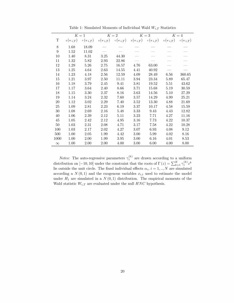
Table 1: Simulated Moments of Individual Wald Wi,T Statistics

K = 1 K = 2 K = 3 K = 4T E(W i,T ) V(W i,T ) E(W i,T ) V(W i,T ) E(W i,T ) V(W i,T ) E(W i,T ) V(W i,T )

8 1.68 18.09 – – – – – –9 1.52 11.02 – – – – – –10 1.40 8.31 3.25 44.30 – – – –11 1.32 5.82 2.93 22.86 – – – –12 1.29 5.26 2.75 16.57 4.76 63.00 – –13 1.25 4.64 2.63 14.55 4.41 40.92 – –14 1.23 4.18 2.56 12.59 4.09 28.49 6.56 360.6515 1.21 3.97 2.50 11.11 3.94 23.34 5.89 65.4716 1.18 3.79 2.45 9.41 3.81 19.52 5.51 43.6217 1.17 3.64 2.40 8.66 3.71 15.68 5.19 30.5918 1.15 3.30 2.37 8.16 3.63 14.56 5.10 27.2919 1.14 3.24 2.32 7.60 3.57 14.29 4.99 25.2120 1.12 3.02 2.29 7.40 3.52 13.30 4.88 21.6925 1.09 2.81 2.23 6.19 3.37 10.17 4.58 15.5930 1.08 2.69 2.16 5.48 3.33 9.43 4.43 12.8240 1.06 2.39 2.12 5.11 3.23 7.71 4.27 11.1645 1.05 2.42 2.12 4.95 3.16 7.73 4.22 10.3750 1.03 2.31 2.08 4.71 3.17 7.58 4.22 10.28100 1.03 2.17 2.02 4.27 3.07 6.93 4.08 9.12500 1.00 2.05 1.99 4.42 3.00 5.99 4.02 8.161000 1.00 2.00 1.99 3.95 3.00 6.16 4.01 8.53∞ 1.00 2.00 2.00 4.00 3.00 6.00 4.00 8.00

Notes: The auto-regressive parameters γ(k)i are drawn according to a uniformdistribution on [−10, 10] under the constraint that the roots of Γ (z) = K

k=1 γ(k)i zk

lie outside the unit circle. The fixed individual effects αi, i = 1, .., N are simulatedaccording a N (0, 1) and the exogenous variables xi,t used to estimate the modelunder H1 are simulated in a N (0, 1) distribution. The empirical moments of theWald statistic Wi,T are evaluated under the null HNC hypothesis.

20

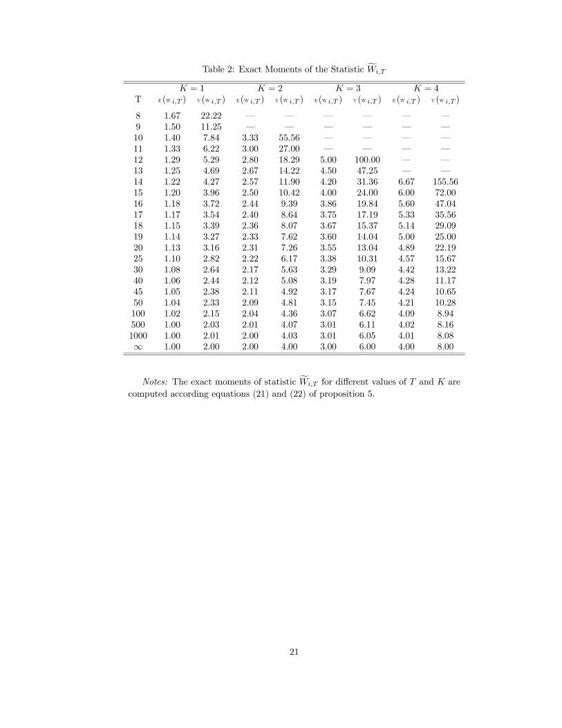
Table 2: Exact Moments of the Statistic Wi,T

K = 1 K = 2 K = 3 K = 4T E(W i,T ) V(W i,T ) E(W i,T ) V(W i,T ) E(W i,T ) V(W i,T ) E(W i,T ) V(W i,T )

8 1.67 22.22 – – – – – –9 1.50 11.25 – – – – – –10 1.40 7.84 3.33 55.56 – – – –11 1.33 6.22 3.00 27.00 – – – –12 1.29 5.29 2.80 18.29 5.00 100.00 – –13 1.25 4.69 2.67 14.22 4.50 47.25 – –14 1.22 4.27 2.57 11.90 4.20 31.36 6.67 155.5615 1.20 3.96 2.50 10.42 4.00 24.00 6.00 72.0016 1.18 3.72 2.44 9.39 3.86 19.84 5.60 47.0417 1.17 3.54 2.40 8.64 3.75 17.19 5.33 35.5618 1.15 3.39 2.36 8.07 3.67 15.37 5.14 29.0919 1.14 3.27 2.33 7.62 3.60 14.04 5.00 25.0020 1.13 3.16 2.31 7.26 3.55 13.04 4.89 22.1925 1.10 2.82 2.22 6.17 3.38 10.31 4.57 15.6730 1.08 2.64 2.17 5.63 3.29 9.09 4.42 13.2240 1.06 2.44 2.12 5.08 3.19 7.97 4.28 11.1745 1.05 2.38 2.11 4.92 3.17 7.67 4.24 10.6550 1.04 2.33 2.09 4.81 3.15 7.45 4.21 10.28100 1.02 2.15 2.04 4.36 3.07 6.62 4.09 8.94500 1.00 2.03 2.01 4.07 3.01 6.11 4.02 8.161000 1.00 2.01 2.00 4.03 3.01 6.05 4.01 8.08∞ 1.00 2.00 2.00 4.00 3.00 6.00 4.00 8.00

Notes: The exact moments of statistic Wi,T for different values of T and K arecomputed according equations (21) and (22) of proposition 5.

21

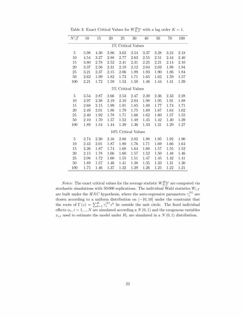
Table 3: Exact Critical Values for WHncN,T with a lag order K = 1.

N\T 10 15 20 25 30 40 50 70 100

1% Critical Values

5 5.98 4.30 3.86 3.62 3.54 3.37 3.28 3.24 3.1810 4.54 3.27 2.88 2.77 2.63 2.55 2.51 2.44 2.4015 3.80 2.78 2.52 2.41 2.31 2.25 2.21 2.14 2.1020 3.37 2.56 2.31 2.19 2.12 2.04 2.03 1.98 1.9425 3.21 2.37 2.15 2.06 1.99 1.93 1.90 1.86 1.8450 2.62 1.99 1.82 1.73 1.71 1.65 1.62 1.59 1.57100 2.21 1.72 1.59 1.53 1.50 1.46 1.44 1.41 1.39

5% Critical Values

5 3.54 2.87 2.66 2.53 2.47 2.39 2.36 2.33 2.2810 2.97 2.38 2.19 2.10 2.04 1.98 1.95 1.91 1.8815 2.68 2.15 1.99 1.91 1.85 1.80 1.77 1.74 1.7120 2.49 2.01 1.86 1.79 1.75 1.69 1.67 1.64 1.6225 2.40 1.92 1.78 1.71 1.66 1.62 1.60 1.57 1.5550 2.10 1.70 1.57 1.52 1.49 1.45 1.42 1.40 1.39100 1.89 1.54 1.44 1.39 1.36 1.33 1.31 1.29 1.27

10% Critical Values

5 2.74 2.30 2.16 2.08 2.02 1.98 1.95 1.92 1.9010 2.43 2.01 1.87 1.80 1.76 1.71 1.69 1.66 1.6415 2.26 1.87 1.74 1.68 1.64 1.60 1.57 1.55 1.5220 2.15 1.78 1.66 1.60 1.57 1.52 1.50 1.48 1.4625 2.08 1.72 1.60 1.55 1.51 1.47 1.45 1.42 1.4150 1.89 1.57 1.46 1.41 1.38 1.35 1.33 1.31 1.30100 1.75 1.46 1.37 1.32 1.29 1.26 1.25 1.22 1.21

Notes: The exact critical values for the average statisticWHncN,T are computed via

stochastic simulations with 50 000 replications. The individual Wald statistics Wi,T

are built under the HNC hypothesis, where the auto-regressive parameters γ(k)i aredrawn according to a uniform distribution on [−10, 10] under the constraint thatthe roots of Γ (z) = K

k=1 γ(k)i zk lie outside the unit circle. The fixed individual

effects αi, i = 1, .., N are simulated according a N (0, 1) and the exogenous variablesxi,t used to estimate the model under H1 are simulated in a N (0, 1) distribution.

22

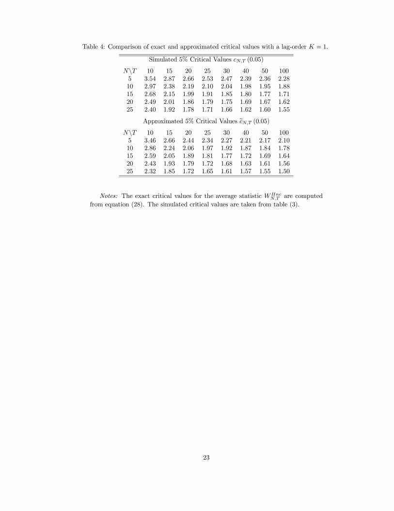
Table 4: Comparison of exact and approximated critical values with a lag-order K = 1.

Simulated 5% Critical Values cN,T (0.05)

N\T 10 15 20 25 30 40 50 1005 3.54 2.87 2.66 2.53 2.47 2.39 2.36 2.2810 2.97 2.38 2.19 2.10 2.04 1.98 1.95 1.8815 2.68 2.15 1.99 1.91 1.85 1.80 1.77 1.7120 2.49 2.01 1.86 1.79 1.75 1.69 1.67 1.6225 2.40 1.92 1.78 1.71 1.66 1.62 1.60 1.55

Approximated 5% Critical Values cN,T (0.05)

N\T 10 15 20 25 30 40 50 1005 3.46 2.66 2.44 2.34 2.27 2.21 2.17 2.1010 2.86 2.24 2.06 1.97 1.92 1.87 1.84 1.7815 2.59 2.05 1.89 1.81 1.77 1.72 1.69 1.6420 2.43 1.93 1.79 1.72 1.68 1.63 1.61 1.5625 2.32 1.85 1.72 1.65 1.61 1.57 1.55 1.50

Notes: The exact critical values for the average statistic WHncN,T are computed

from equation (28). The simulated critical values are taken from table (3).

23