Testing for additivity in nonparametric quantile regression · 2015-08-20 · Testing for additivity in nonparametric quantile regression Holger Dette, Matthias Guhlich Ruhr-Universit

Testing for additivity in nonparametric quantile

regression

Holger Dette, Matthias Guhlich

Ruhr-Universitat Bochum

Fakultat fur Mathematik

44780 Bochum, Germany

e-mail: [email protected]

Natalie Neumeyer

Universitat Hamburg

Fachbereich Mathematik

20146 Hamburg, Germany

e-mail: [email protected]

December 22, 2011

Abstract

In this article we propose a new test for additivity in nonparametric quantile regression

with a high dimensional predictor. Asymptotic normality of the corresponding test statistic

(after appropriate standardization) is established under the null hypothesis, local and fixed

alternatives. We also propose a bootstrap procedure which can be used to improve the

approximation of the nominal level for moderate sample sizes. The methodology is also

illustrated by means of a small simulation study, and a data example is analyzed.

AMS Subject Classification: 62G05, 62G20

Keywords and Phrases: nonparametric regression, quantile regression, bootstrap, additive estima-

tion

1 Introduction

Quantile regression was introduced by Koenker and Bassett (1978) as a complement to least

squares estimation (LSE) or maximum likelihood estimation (MLE) and leads to far-reaching ex-

tensions of “classical” regression analysis by estimating families of conditional quantile surfaces,

which describe the relation between a one-dimensional response y and a high dimensional predic-

tor x. Since its introduction it has found great attraction in mathematical and applied statistics

because of its ease of interpretation and robustness, which yields attractive applications in such

important areas as medicine, economics, engineering and environmental modeling. The interested

reader is referred to the recent monograph of Koenker (2005). Many authors consider parametric

1

quantile regression models but in the last two decades nonparametric methods for estimating con-

ditional quantiles have also been discussed intensively. Most of the literature refers to models with

a univariate predictor [see e.g. Yu and Jones (1997), Yu and Jones (1998), Dette and Volgushev

(2008) and Chernozhukov et al. (2010)]. While from a theoretical point of view there is no difficulty

to generalize this methodology to high-dimensional covariates, it is well known that in practical

applications such nonparametric methods suffer from the curse of dimensionality and therefore do

not yield precise estimates of conditional quantile surfaces for reasonable sample sizes. A common

approach in nonparametric statistics to deal with this problem is to postulate an additive non-

parametric model, which allows the estimation of the regression with one-dimensional rates. In

classical regression (estimating the conditional expectation of the response given in the predictor)

this methodology has found considerable interest in the literature [see Linton and Nielsen (1995),

Mammen et al. (1999), Carroll et al. (2002), Hengartner and Sperlich (2005), Nielsen and Sperlich

(2005), among others]. In quantile regression nonparametric models of this type have only been

discussed more recently. Doksum and Koo (2000) suggest a spline estimate and De Gooijer and

Zerom (2003) introduce a marginal integration estimate of an additive quantile regression model.

Horowitz and Lee (2005) propose a two step procedure, which fits a parametric model in the

first step (with increasing dimension) for each coordinate and smooth it in a second step by the

local polynomial technique. Lee et al. (2010) suggest backfitting methods for additive quantile

regression estimation, while Dette and Scheder (2011) combine marginal integration techniques

with monotone rearrangements [see Dette et al. (2006)] for the construction of additive estimates.

Although these methods estimate the unknown quantile regression with the optimal (one-dimensional)

rate if the assumption of an additive model is correct, they are generally inconsistent if the quan-

tile regression is not additive. In this case the corresponding statistics usually estimate a “best

approximation” of the unknown regression by an additive quantile regression model, but the dif-

ference between the “true” curve and its best approximation can be substantial. For this reason,

it is of some importance to investigate by a statistical test if the hypothesis of an additive quantile

regression is satisfied. In the context of modeling the conditional expectation this problem has

found considerable interest in the literature [see for example Eubank et al. (1995), Gozalo and

Linton (2001), Dette and von Lieres und Wilkau (2001), Derbort et al. (2002) or Abramovich

et al. (2009), among others]. On the other hand, to the best knowledge of the authors, tests

for the hypothesis of an additive quantile regression model have not been considered so far in

the literature, and the purpose of the present paper is to propose and analyze such a procedure

for this problem. In Section 2 we introduce the basic notation and an additive estimate of the

conditional quantile curve. The test statistic for the problem of additive quantile regression uses

the residuals from this additive fit and is introduced in Section 3, where we also study the main

asymptotic properties. In particular, we prove weak convergence of an appropriately standardized

version of the test statistic under the null hypothesis and fixed alternatives with different rates

corresponding to both cases. In Section 4 we present a small simulation study in order to illustrate

the finite sample properties of a bootstrap version of the proposed test. We also investigate a data

2

example testing if the hypothesis of an additive quantile regression is satisfied. Finally, all proofs

and some of the more technical details in the proofs are deferred to an appendix in Section 5, 6

and 7.

2 Preliminaries - an additive estimator

Consider a sequence of independent identically distributed observations (X1, Y1), . . . , (Xn, Yn)

where Xj = (Xj1, . . . , Xjd)T denotes a d−dimensional random variable with density f and fi

is the marginal density of the ith component Xji of Xj (i = 1, . . . , d). Throughout this paper we

denote by F (y|x) the conditional distribution function of Y1 given X1 = x = (x1, . . . , xd)T and by

Q(τ |x) = F−1(y|x) the corresponding conditional quantile function. In the following we fix some

τ ∈ (0, 1) and are interested in the problem of testing the hypothesis of additivity

(2.1) H0 : Q(τ |x) = Q(τ |x1, . . . , xd) =d∑

k=1

Qk(τ |xk) + c(τ)

for some constant c(τ) and functions Qk(τ |xk) (k = 1, . . . , d). Note that the quantities in (2.1)

are not uniquely determined and in order to make these identifiable we assume throughout this

paper the conditions

E[Qk(τ |Xjk)] = 0, k = 1, . . . , d, j = 1, . . . , n.

For the construction of a test for the hypothesis (2.1) let Qadd denote an additive estimate of the

quantile regression function Q (for fixed τ), which will be specified later. We propose the statistic

(2.2) Tn =1

n(n− 1)

n∑i=1

n∑j 6=i

Lg (Xi −Xj) RiRj,

where the random variables Ri are defined by

(2.3) Ri = IYi ≤ Q−iadd(τ |Xi) − τ,

the function L denotes a d-dimensional kernel function with bandwidth g and here and throughout

this paper we use the notation

Lg(Xi −Xj) =1

gdL(Xi −Xj

g

).(2.4)

Throughout this paper we use the notation a and a−i corresponding to estimates from the full

sample (Xj, Yj)|j = 1, . . . , n and the sample without the ith observation, respectively. Thus the

statistic Q−iadd(τ |x) in (2.3) denotes the additive (nonparametric) estimate of the quantile regression

from the sample without the ith observation. Similarly, Q−i,jadd and Q−i,j,kadd denote the corresponding

3

estimators without the ith and jth and the ith, jth and kth observation, respectively. Various ad-

ditive quantile regression estimates have been proposed by De Gooijer and Zerom (2003), Horowitz

and Lee (2005), Lee et al. (2010) and Dette and Scheder (2011).

Note that statistics of the type (2.4) have been introduced by Zheng (1996) in the context of

testing for a specific parametric form in nonparametric regression, and since its introduction has

found considerable interest in the context of goodness-of-fit tests [see Dette and von Lieres und

Wilkau (2001) or Zhang and Dette (2004) among others]. In the following section we will study the

asymptotic properties of the test statistic under the null hypothesis of additivity, local alternatives

and fixed alternatives. In particular, we prove weak convergence of a standardized version of the

statistic Tn defined in (2.2) with different rates corresponding to the null hypothesis and fixed

alternatives. For this discussion which is deferred to Section 3 we therefore recall the definition of

an additive quantile regression estimate which has recently been introduced by Dette and Scheder

(2010) and will be used throughout this paper for a test of an additive quantile regression. Let

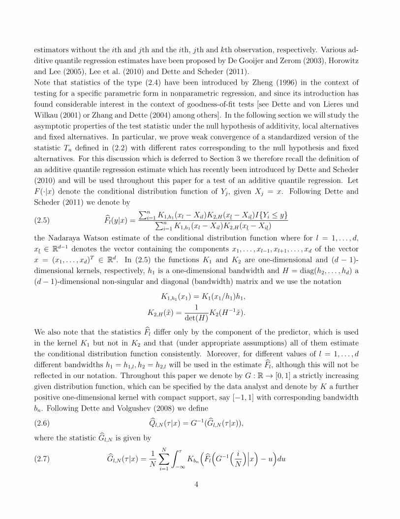
F (·|x) denote the conditional distribution function of Yj, given Xj = x. Following Dette and

Scheder (2011) we denote by

(2.5) Fl(y|x) =

∑ni=1K1,h1(xl −Xil)K2,H(xl −Xil)IYi ≤ y∑n

i=1K1,h1(xl −Xil)K2,H(xl −Xil)

the Nadaraya Watson estimate of the conditional distribution function where for l = 1, . . . , d,

xl ∈ Rd−1 denotes the vector containing the components x1, . . . , xl−1, xl+1, . . . , xd of the vector

x = (x1, . . . , xd)T ∈ Rd. In (2.5) the functions K1 and K2 are one-dimensional and (d − 1)-

dimensional kernels, respectively, h1 is a one-dimensional bandwidth and H = diag(h2, . . . , hd) a

(d− 1)-dimensional non-singular and diagonal (bandwidth) matrix and we use the notation

K1,h1(x1) = K1(x1/h1)h1,

K2,H(x) =1

det(H)K2(H

−1x).

We also note that the statistics Fl differ only by the component of the predictor, which is used

in the kernel K1 but not in K2 and that (under appropriate assumptions) all of them estimate

the conditional distribution function consistently. Moreover, for different values of l = 1, . . . , d

different bandwidths h1 = h1,l, h2 = h2,l will be used in the estimate Fl, although this will not be

reflected in our notation. Throughout this paper we denote by G : R→ [0, 1] a strictly increasing

given distribution function, which can be specified by the data analyst and denote by K a further

positive one-dimensional kernel with compact support, say [−1, 1] with corresponding bandwidth

bn. Following Dette and Volgushev (2008) we define

(2.6) Ql,N(τ |x) = G−1(Gl,N(τ |x)),

where the statistic Gl,N is given by

(2.7) Gl,N(τ |x) =1

N

N∑i=1

∫ τ

−∞Kbn

(Fl

(G−1

( iN

)∣∣∣x)− u)du4

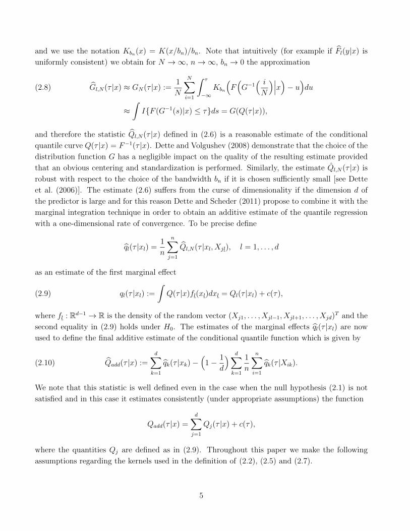
and we use the notation Kbn(x) = K(x/bn)/bn. Note that intuitively (for example if Fl(y|x) is

uniformly consistent) we obtain for N →∞, n→∞, bn → 0 the approximation

Gl,N(τ |x) ≈ GN(τ |x) :=1

N

N∑i=1

∫ τ

−∞Kbn

(F(G−1

( iN

)∣∣∣x)− u)du(2.8)

≈∫IF (G−1(s)|x) ≤ τds = G(Q(τ |x)),

and therefore the statistic Ql,N(τ |x) defined in (2.6) is a reasonable estimate of the conditional

quantile curve Q(τ |x) = F−1(τ |x). Dette and Volgushev (2008) demonstrate that the choice of the

distribution function G has a negligible impact on the quality of the resulting estimate provided

that an obvious centering and standardization is performed. Similarly, the estimate Ql,N(τ |x) is

robust with respect to the choice of the bandwidth bn if it is chosen sufficiently small [see Dette

et al. (2006)]. The estimate (2.6) suffers from the curse of dimensionality if the dimension d of

the predictor is large and for this reason Dette and Scheder (2011) propose to combine it with the

marginal integration technique in order to obtain an additive estimate of the quantile regression

with a one-dimensional rate of convergence. To be precise define

ql(τ |xl) =1

n

n∑j=1

Ql,N(τ |xl, Xjl), l = 1, . . . , d

as an estimate of the first marginal effect

ql(τ |xl) :=

∫Q(τ |x)fl(xl)dxl = Ql(τ |xl) + c(τ),(2.9)

where fl : Rd−1 → R is the density of the random vector (Xj1, . . . , Xjl−1, Xjl+1, . . . , Xjd)T and the

second equality in (2.9) holds under H0. The estimates of the marginal effects ql(τ |xl) are now

used to define the final additive estimate of the conditional quantile function which is given by

(2.10) Qadd(τ |x) :=d∑

k=1

qk(τ |xk)−(

1− 1

d

) d∑k=1

1

n

n∑i=1

qk(τ |Xik).

We note that this statistic is well defined even in the case when the null hypothesis (2.1) is not

satisfied and in this case it estimates consistently (under appropriate assumptions) the function

Qadd(τ |x) =d∑j=1

Qj(τ |x) + c(τ),

where the quantities Qj are defined as in (2.9). Throughout this paper we make the following

assumptions regarding the kernels used in the definition of (2.2), (2.5) and (2.7).

5

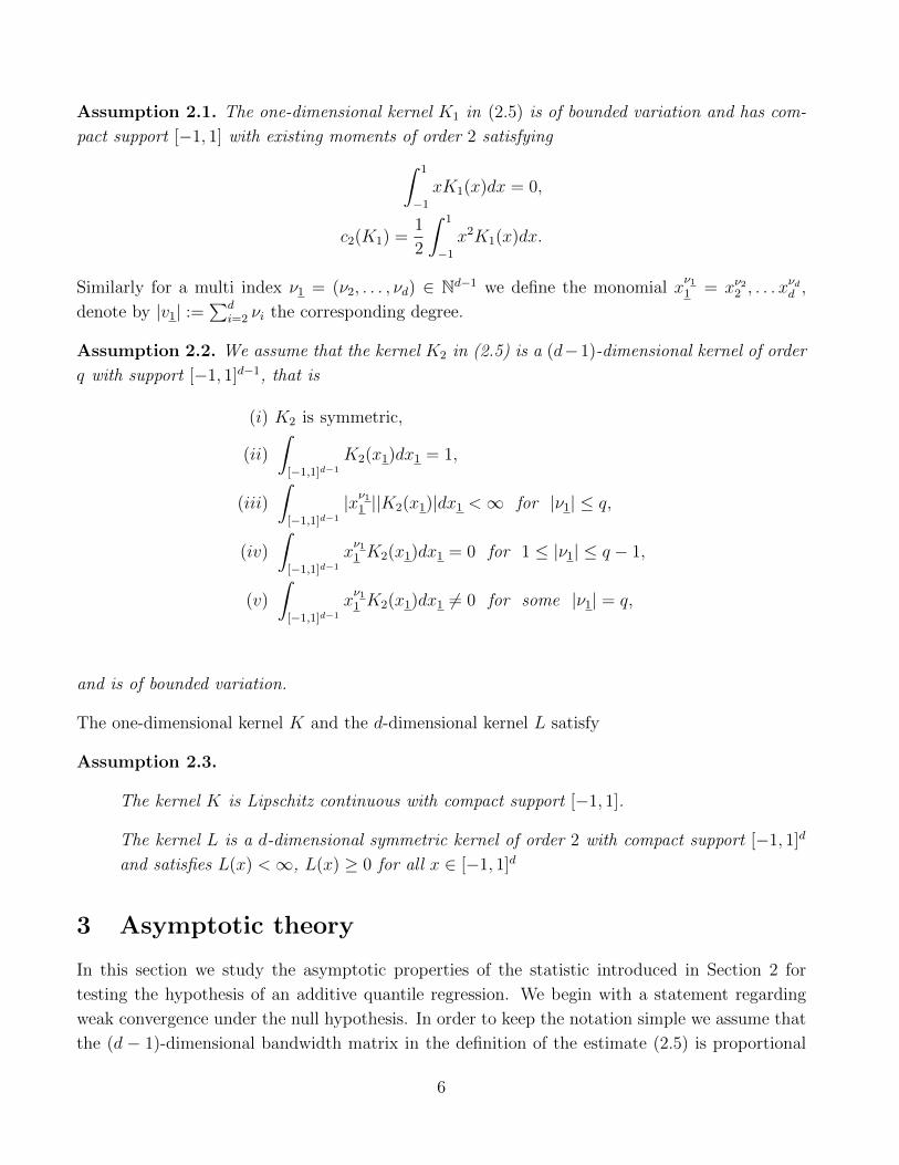
Assumption 2.1. The one-dimensional kernel K1 in (2.5) is of bounded variation and has com-

pact support [−1, 1] with existing moments of order 2 satisfying∫ 1

−1xK1(x)dx = 0,

c2(K1) =1

2

∫ 1

−1x2K1(x)dx.

Similarly for a multi index ν1 = (ν2, . . . , νd) ∈ Nd−1 we define the monomial xν11 = xν22 , . . . x

νdd ,

denote by |v1| :=∑d

i=2 νi the corresponding degree.

Assumption 2.2. We assume that the kernel K2 in (2.5) is a (d−1)-dimensional kernel of order

q with support [−1, 1]d−1, that is

(i) K2 is symmetric,

(ii)

∫[−1,1]d−1

K2(x1)dx1 = 1,

(iii)

∫[−1,1]d−1

|xν11 ||K2(x1)|dx1 <∞ for |ν1| ≤ q,

(iv)

∫[−1,1]d−1

xν11 K2(x1)dx1 = 0 for 1 ≤ |ν1| ≤ q − 1,

(v)

∫[−1,1]d−1

xν11 K2(x1)dx1 6= 0 for some |ν1| = q,

and is of bounded variation.

The one-dimensional kernel K and the d-dimensional kernel L satisfy

Assumption 2.3.

The kernel K is Lipschitz continuous with compact support [−1, 1].

The kernel L is a d-dimensional symmetric kernel of order 2 with compact support [−1, 1]d

and satisfies L(x) <∞, L(x) ≥ 0 for all x ∈ [−1, 1]d

3 Asymptotic theory

In this section we study the asymptotic properties of the statistic introduced in Section 2 for

testing the hypothesis of an additive quantile regression. We begin with a statement regarding

weak convergence under the null hypothesis. In order to keep the notation simple we assume that

the (d − 1)-dimensional bandwidth matrix in the definition of the estimate (2.5) is proportional

6

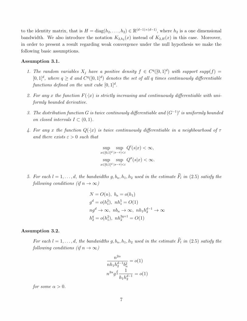
to the identity matrix, that is H = diag(h2, . . . , h2) ∈ R(d−1)×(d−1), where h2 is a one dimensional

bandwidth. We also introduce the notation K2,h2(x) instead of K2,H(x) in this case. Moreover,

in order to present a result regarding weak convergence under the null hypothesis we make the

following basic assumptions.

Assumption 3.1.

1. The random variables Xj have a positive density f ∈ Cq([0, 1]d) with support supp(f) =

[0, 1]d, where q ≥ d and Cq([0, 1]d) denotes the set of all q times continuously differentiable

functions defined on the unit cube [0, 1]d.

2. For any x the function F (·|x) is strictly increasing and continuously differentiable with uni-

formly bounded derivative.

3. The distribution function G is twice continously differentiable and (G−1)′ is uniformly bounded

on closed intervals I ⊂ (0, 1).

4. For any x the function Q(·|x) is twice continuously differentiable in a neighbourhood of τ

and there exists ε > 0 such that

supx∈[0,1]d

sup|s−τ |<ε

Q′(s|x) <∞,

supx∈[0,1]d

sup|s−τ |<ε

Q′′(s|x) <∞.

5. For each l = 1, . . . , d, the bandwidths g, bn, h1, h2 used in the estimate Fl in (2.5) satisfy the

following conditions (if n→∞)

N = O(n), bn = o(h1)

gd = o(h21), nh51 = O(1)

ngd →∞, nbn →∞, nh1hd−12 →∞hq2 = o(h21), nh

2q+12 = O(1)

Assumption 3.2.

For each l = 1, . . . , d, the bandwidths g, bn, h1, h2 used in the estimate Fl in (2.5) satisfy the


n2α

nh1hd−12 b2n

= o(1)

n2αgd2

1

h1hd−12

= o(1)

for some α > 0.

7

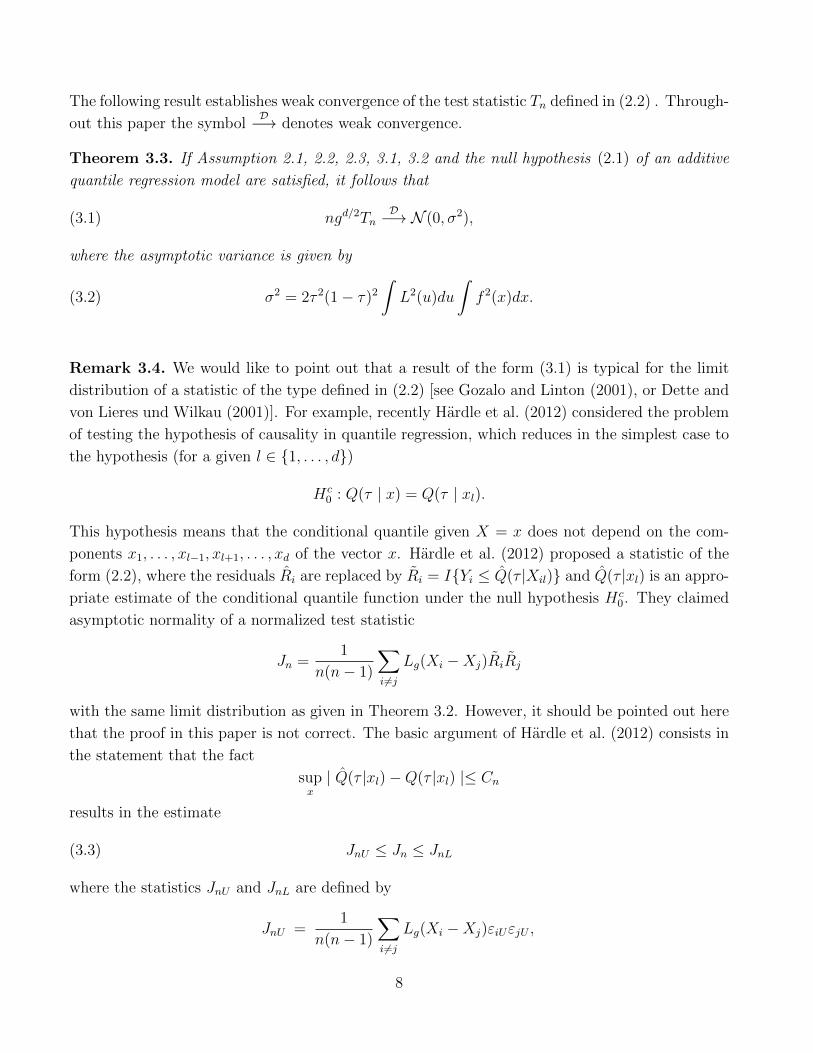
The following result establishes weak convergence of the test statistic Tn defined in (2.2) . Through-

out this paper the symbolD−→ denotes weak convergence.

Theorem 3.3. If Assumption 2.1, 2.2, 2.3, 3.1, 3.2 and the null hypothesis (2.1) of an additive

quantile regression model are satisfied, it follows that

(3.1) ngd/2TnD−→ N (0, σ2),

where the asymptotic variance is given by

(3.2) σ2 = 2τ 2(1− τ)2∫L2(u)du

∫f 2(x)dx.

Remark 3.4. We would like to point out that a result of the form (3.1) is typical for the limit

distribution of a statistic of the type defined in (2.2) [see Gozalo and Linton (2001), or Dette and

von Lieres und Wilkau (2001)]. For example, recently Hardle et al. (2012) considered the problem

of testing the hypothesis of causality in quantile regression, which reduces in the simplest case to

the hypothesis (for a given l ∈ 1, . . . , d)

Hc0 : Q(τ | x) = Q(τ | xl).

This hypothesis means that the conditional quantile given X = x does not depend on the com-

ponents x1, . . . , xl−1, xl+1, . . . , xd of the vector x. Hardle et al. (2012) proposed a statistic of the

form (2.2), where the residuals Ri are replaced by Ri = IYi ≤ Q(τ |Xil) and Q(τ |xl) is an appro-

priate estimate of the conditional quantile function under the null hypothesis Hc0. They claimed

asymptotic normality of a normalized test statistic

Jn =1

n(n− 1)

∑i 6=j

Lg(Xi −Xj)RiRj

with the same limit distribution as given in Theorem 3.2. However, it should be pointed out here

that the proof in this paper is not correct. The basic argument of Hardle et al. (2012) consists in

the statement that the fact

supx| Q(τ |xl)−Q(τ |xl) |≤ Cn

results in the estimate

(3.3) JnU ≤ Jn ≤ JnL

where the statistics JnU and JnL are defined by

JnU =1

n(n− 1)

∑i 6=j

Lg(Xi −Xj)εiUεjU ,

8

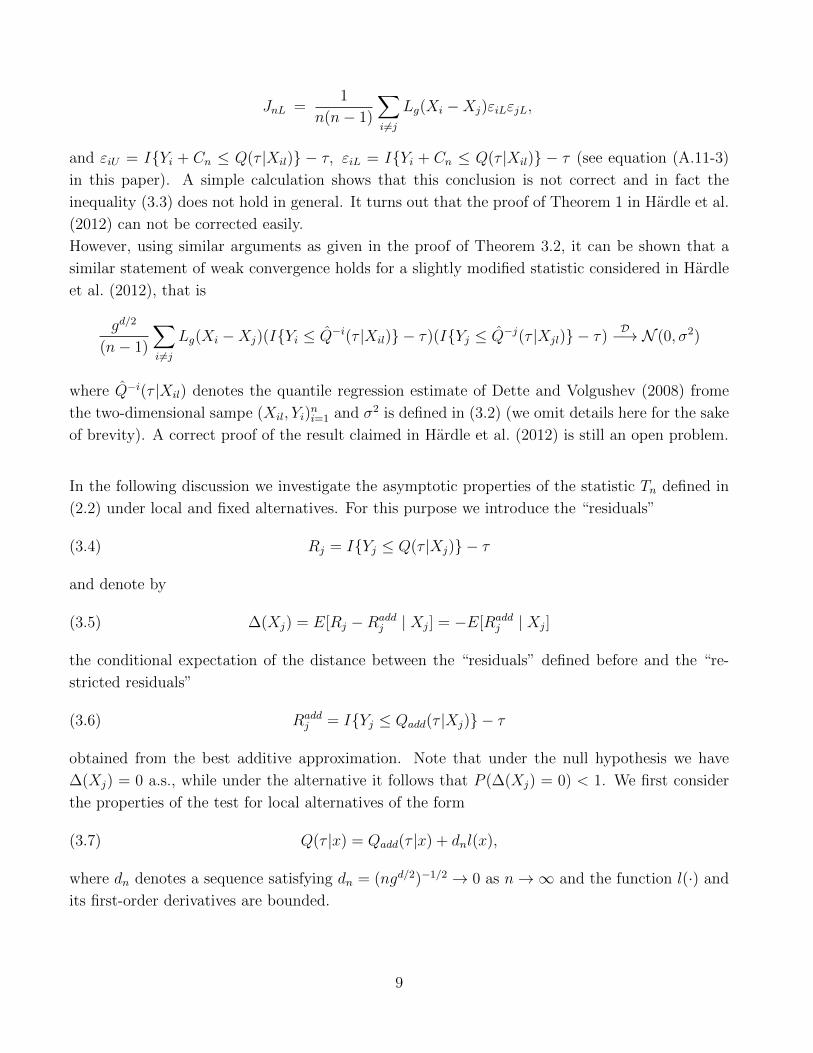
JnL =1

n(n− 1)

∑i 6=j

Lg(Xi −Xj)εiLεjL,

and εiU = IYi + Cn ≤ Q(τ |Xil) − τ, εiL = IYi + Cn ≤ Q(τ |Xil) − τ (see equation (A.11-3)

in this paper). A simple calculation shows that this conclusion is not correct and in fact the

inequality (3.3) does not hold in general. It turns out that the proof of Theorem 1 in Hardle et al.

(2012) can not be corrected easily.

However, using similar arguments as given in the proof of Theorem 3.2, it can be shown that a

similar statement of weak convergence holds for a slightly modified statistic considered in Hardle

et al. (2012), that is

gd/2

(n− 1)

∑i 6=j

Lg(Xi −Xj)(IYi ≤ Q−i(τ |Xil) − τ)(IYj ≤ Q−j(τ |Xjl) − τ)D−→ N (0, σ2)

where Q−i(τ |Xil) denotes the quantile regression estimate of Dette and Volgushev (2008) frome

the two-dimensional sampe (Xil, Yi)ni=1 and σ2 is defined in (3.2) (we omit details here for the sake

of brevity). A correct proof of the result claimed in Hardle et al. (2012) is still an open problem.

In the following discussion we investigate the asymptotic properties of the statistic Tn defined in

(2.2) under local and fixed alternatives. For this purpose we introduce the “residuals”

(3.4) Rj = IYj ≤ Q(τ |Xj) − τ

and denote by

(3.5) ∆(Xj) = E[Rj −Raddj | Xj] = −E[Radd

j | Xj]

the conditional expectation of the distance between the “residuals” defined before and the “re-

stricted residuals”

(3.6) Raddj = IYj ≤ Qadd(τ |Xj) − τ

obtained from the best additive approximation. Note that under the null hypothesis we have

∆(Xj) = 0 a.s., while under the alternative it follows that P (∆(Xj) = 0) < 1. We first consider

the properties of the test for local alternatives of the form

(3.7) Q(τ |x) = Qadd(τ |x) + dnl(x),

where dn denotes a sequence satisfying dn = (ngd/2)−1/2 → 0 as n→∞ and the function l(·) and

its first-order derivatives are bounded.

9

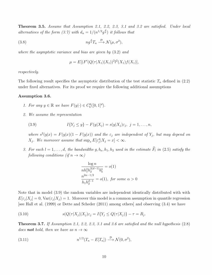
Theorem 3.5. Assume that Assumption 2.1, 2.2, 2.3, 3.1 and 3.2 are satisfied. Under local

alternatives of the form (3.7) with dn = 1/(n1/2gd4 ) it follows that

(3.8) ngd2Tn

D−→ N (µ, σ2),

where the asymptotic variance and bias are given by (3.2) and

µ = E[(F ′(Q(τ |X1)|X1))2l2(X1)f(X1)],

respectively.

The following result specifies the asymptotic distribution of the test statistic Tn defined in (2.2)

under fixed alternatives. For its proof we require the following additional assumptions

Assumption 3.6.

1. For any y ∈ R we have F (y|·) ∈ Cqb ([0, 1]d).

2. We assume the representation

IYj ≤ y − F (y|Xj) = s(y|Xj)εj, j = 1, . . . , n,(3.9)

where s2(y|x) = F (y|x)(1 − F (y|x)) and the εj are independent of Yj, but may depend on

Xj. We moreover assume that supxE[ε4j |Xj = x] <∞.

3. For each l = 1, . . . , d, the bandwidths g, bn, h1, h2 used in the estimate Fl in (2.5) satisfy the


log n

nh21h2(d−1)2 b2n

= o(1)

n2α−1/2

h1hd−12

= o(1), for some α > 0

Note that in model (3.9) the random variables are independent identically distributed with with

E[εj|Xj] = 0, Var(εj|Xj) = 1. Moreover this model is a common assumption in quantile regression

[see Hall et al. (1999) or Dette and Scheder (2011) among others] and observing (3.4) we have

(3.10) s(Q(τ |Xj)|Xj)εj = IYj ≤ Q(τ |Xj) − τ = Rj.

Theorem 3.7. If Assumption 2.1, 2.2, 2.3, 3.1 and 3.6 are satisfied and the null hypothesis (2.8)

does not hold, then we have as n→∞

(3.11) n1/2(Tn − E[Tn])D−→ N (0, σ2),

10

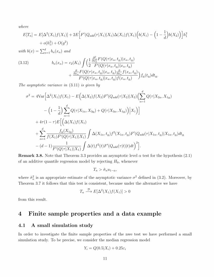
where

E[Tn] = E[∆2(X1)f(X1)] + 2E[F ′(Qadd(τ |X1)|X1)∆(X1)f(X1)

(b(X1)−

(1− 1

d

)b(X2)

)]h21

+ o(h21) +O(g2)

with b(x) =∑d

α=1 bα(xα) and

bα(xα) = c2(K1)

∫ (1

2

∂2

∂x2αF (Q(τ |xα, tα)|xα, tα)

F ′(Q(τ |xα, tα)|xα, tα)(3.12)

+∂∂xα

F (Q(τ |xα, tα)|xα, tα) ∂∂xα

f(xα, tα)

F ′(Q(τ |xα, tα)|xα, tα)f(xα, tα)

)fα(tα)dtα.

The asymptotic variance in (3.11) is given by

σ2 = 4Var[∆2(X1)f(X1)− E

(∆(X2)f(X2)F

′(Qadd(τ |X2)|X2)( d∑α=1

Q(τ |X2α, X1α)

−(

1− 1

d

) d∑α=1

Q(τ |X1α, X3α) +Q(τ |X3α, X1α))∣∣∣X1

)]+ 4τ(1− τ)E

[(∆(X1)f(X1)

+d∑

α=1

fα(X1α)

f(X1)F ′(Q(τ |X1)|X1)

∫∆(X1α, tα)f 2(X1α, tα)F ′(Qadd(τ |X1α, tα)|X1α, tα)dtα

− (d− 1)1

F ′(Q(τ |X1)|X1)

∫∆(t)f 2(t)F ′(Qadd(τ |t)|t)dt

)2].

Remark 3.8. Note that Theorem 3.3 provides an asymptotic level α test for the hypothesis (2.1)

of an additive quantile regression model by rejecting H0, whenever

Tn > σnu1−α,

where σ2n is an appropriate estimate of the asymptotic variance σ2 defined in (3.2). Moreover, by

Theorem 3.7 it follows that this test is consistent, because under the alternative we have

TnD−→ E[∆2(X1)f(X1)] > 0

from this result.

4 Finite sample properties and a data example

4.1 A small simulation study

In order to investigate the finite sample properties of the nwe test we have performed a small

simulation study. To be precise, we consider the median regression model

Yi = Q(0.5|Xi) + 0.25εi

11

where εi are independent, standard normally distributed and independent of the bivariate covari-

ates Xi = (Xi1, Xi2), i = 1, . . . , n. For the choice of the predictor we investigate the following two

scenarios.

(A) Xi are uniformly distributed on the unit square [0, 1]2

Xi = (Xi1, Xi2) ∼ U([0, 1]2), i = 1, . . . , n

(B) Xi = (Xi1, Xi2) are given by

Xi1 =1

2+

1

πarctan(Zi1)

Xi2 =1

2+

1

πarctan(Zi2)

where Zi = (Zi1, Zi2) are (independent) centered normally distributed random variables with

variance 1 and correlation ρ = 0.2, ρ = 0.5, ρ = 0.8.

Note that in Design A the random variables Xi1 and Xi2 are independent, whereas Design B

represents a situation where Xi1 and Xi2 are correlated. In our simulation study we consider three

models for the conditional quantile function, that is

Q(0.5|x1, x2) = x1 + x2(4.1)

Q(0.5|x1, x2) = x21 + x22(4.2)

Q(0.5|x1, x2) = cos(cπ(x1 + x2)), c = 0.5, 1, 2,(4.3)

where the first two cases correspond to the null hypothesis of additivity and (4.3) represents

three alternatives. For all kernels in our estimators we use the Epanechnikov kernel K(t) =34(1− t2)I[−1,1](t), and a product of two kernels of this type as a two-dimensional kernel. Following

Dette and Scheder (2011) the bandwidths are chosen as

h1 = 0.6n−15 , h2 = 0.2n−

15 , bn = 0.1n−

14 , g = 0.1n−

14 .

In similar problems it has been observed by several authors [see Fan and Linton (2003)] that

the asymptotic normal distribution under the null hypothesis does not provide a satisfactory

approximation for the distribution of the statistic Tn for small sample sizes. For this reason many

authors propose the application of a bootstrap in this context to calculate critical values. We

follow this suggestion and use a wild bootstrap for this purpose. To be precise, in the τ -quantile

model we define a bootstrap sample by

Y ∗i = Qadd(τ |Xi) + vi|Yi − QN(τ |Xi)|,

where Qadd and QN are defined in Section 2 and vi denote independent identically distributed

random variables satisfying P (vi = −1) = τ and P (vi = 1) = 1 − τ , which are independent

12

from the original sample. A similar bootstrap data generation was suggested by Sun (2006) The

bootstrap observations, conditionally on the original sample, fulfill H0 and additionally fulfill a

τ -quantile regression model because

P ∗(Y ∗i ≤ Qadd(τ |Xi) | Xi = x) = P (vi ≤ 0) = τ,

where P ∗ denotes the probability conditionally on (Xj, Yj), j = 1, . . . , n. Note also that for the

median model used in the simulations we have τ = 12

and vi are Rademacher variables. The

critical value for the test is then obtained from the bootstrap distribution

P ∗(T ∗n ≥ t∗n,(1−α)) = 1− α,

and the hypothesis of additivity is rejected if Tn ≥ t∗n,(1−α). For the estimation of t∗n,(1−α) we choose

the number of bootstrap replications as B = 100 and we have simulated the rejection probabilities

of this test on the basis of 1000 replications of each experiment.

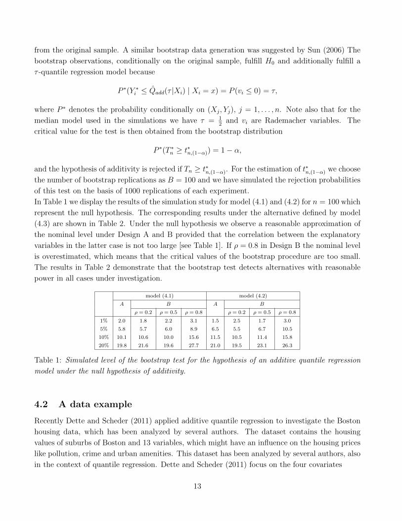
In Table 1 we display the results of the simulation study for model (4.1) and (4.2) for n = 100 which

represent the null hypothesis. The corresponding results under the alternative defined by model

(4.3) are shown in Table 2. Under the null hypothesis we observe a reasonable approximation of

the nominal level under Design A and B provided that the correlation between the explanatory

variables in the latter case is not too large [see Table 1]. If ρ = 0.8 in Design B the nominal level

is overestimated, which means that the critical values of the bootstrap procedure are too small.

The results in Table 2 demonstrate that the bootstrap test detects alternatives with reasonable

power in all cases under investigation.

model (4.1) model (4.2)

A B A B

ρ = 0.2 ρ = 0.5 ρ = 0.8 ρ = 0.2 ρ = 0.5 ρ = 0.8

1% 2.0 1.8 2.2 3.1 1.5 2.5 1.7 3.0

5% 5.8 5.7 6.0 8.9 6.5 5.5 6.7 10.5

10% 10.1 10.6 10.0 15.6 11.5 10.5 11.4 15.8

20% 19.8 21.6 19.6 27.7 21.0 19.5 23.1 26.3

Table 1: Simulated level of the bootstrap test for the hypothesis of an additive quantile regression

model under the null hypothesis of additivity.

4.2 A data example

Recently Dette and Scheder (2011) applied additive quantile regression to investigate the Boston

housing data, which has been analyzed by several authors. The dataset contains the housing

values of suburbs of Boston and 13 variables, which might have an influence on the housing prices

like pollution, crime and urban amenities. This dataset has been analyzed by several authors, also

in the context of quantile regression. Dette and Scheder (2011) focus on the four covariates

13

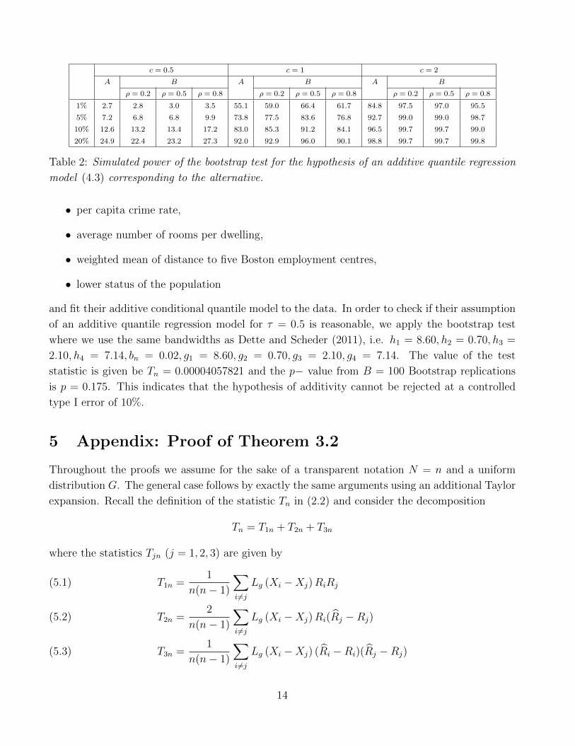
c = 0.5 c = 1 c = 2

A B A B A B

ρ = 0.2 ρ = 0.5 ρ = 0.8 ρ = 0.2 ρ = 0.5 ρ = 0.8 ρ = 0.2 ρ = 0.5 ρ = 0.8

1% 2.7 2.8 3.0 3.5 55.1 59.0 66.4 61.7 84.8 97.5 97.0 95.5

5% 7.2 6.8 6.8 9.9 73.8 77.5 83.6 76.8 92.7 99.0 99.0 98.7

10% 12.6 13.2 13.4 17.2 83.0 85.3 91.2 84.1 96.5 99.7 99.7 99.0

20% 24.9 22.4 23.2 27.3 92.0 92.9 96.0 90.1 98.8 99.7 99.7 99.8

Table 2: Simulated power of the bootstrap test for the hypothesis of an additive quantile regression

model (4.3) corresponding to the alternative.

• per capita crime rate,

• average number of rooms per dwelling,

• weighted mean of distance to five Boston employment centres,

• lower status of the population

and fit their additive conditional quantile model to the data. In order to check if their assumption

of an additive quantile regression model for τ = 0.5 is reasonable, we apply the bootstrap test

where we use the same bandwidths as Dette and Scheder (2011), i.e. h1 = 8.60, h2 = 0.70, h3 =

2.10, h4 = 7.14, bn = 0.02, g1 = 8.60, g2 = 0.70, g3 = 2.10, g4 = 7.14. The value of the test

statistic is given be Tn = 0.00004057821 and the p− value from B = 100 Bootstrap replications

is p = 0.175. This indicates that the hypothesis of additivity cannot be rejected at a controlled

type I error of 10%.

5 Appendix: Proof of Theorem 3.2

Throughout the proofs we assume for the sake of a transparent notation N = n and a uniform

distribution G. The general case follows by exactly the same arguments using an additional Taylor

expansion. Recall the definition of the statistic Tn in (2.2) and consider the decomposition

Tn = T1n + T2n + T3n

where the statistics Tjn (j = 1, 2, 3) are given by

T1n =1

n(n− 1)

∑i 6=j

Lg (Xi −Xj)RiRj(5.1)

T2n =2

n(n− 1)

∑i 6=j

Lg (Xi −Xj)Ri(Rj −Rj)(5.2)

T3n =1

n(n− 1)

∑i 6=j

Lg (Xi −Xj) (Ri −Ri)(Rj −Rj)(5.3)

14

and Ri and Ri are defined in (3.4) and (2.3), respectively. The assertion follows from the following

two statements, which are proved below

ngd2T1n

D−→ N(0, σ2)(5.4)

ngd2Tjn = op(1), j = 2, 3.(5.5)

5.1 Proof of (5.4)

Defining Zi = (Xi, Yi), i = 1, . . . , n, and

Hn(Zi, Zj) = Lg (Xi −Xj) (IYi ≤ Q(τ |Xi) − τ)(IYj ≤ Q(τ |Xj) − τ)

we can write the the statistic ngd2T1n as

ngd2T1n =

gd/2

n− 1

n∑i=1

∑j 6=i

Hn(Zi, Zj)

The assertion then follows from Theorem 1 in Hall (1984) if the assumptions of this statement

can be checked. For this purpose note that we obtain from Assumption 3.2 for i 6= j 6= k 6= i for

some λ > 0

E[E[Hn(Zk, Zi)Hn(Zk, Zj)|Zi, Zj]2]

≤ λ

g4dE[E[L(Xk −Xi

g

)L(Xk −Xj

g

)|Xi, Xj

]2]=

λ

g4d

∫ ∫ [∫L(u)L(u+ v)f(x+ ug)gddu

]2f(x)f(x− vg)gddxdv = O

( 1

gd

)E[H2

n(Zi, Zj)] = τ 2(1− τ)21

g2dE[L2(Xi −Xj

g

)]= τ 2(1− τ)2

1

gd

∫L2(u)du

∫f 2(x)dx+ o

( 1

gd

)=

σ2

2gd+ o( 1

gd

),

where σ2 > 0 is defined in (3.2). In a similar way one establishes the estimate E[H4n(Zi, Zj)] =

O(

1g3d

), which gives

E[E[Hn(Zk, Zi)Hn(Zk, Zj)|Zi, Zj]2] + n−1E[H4n(Zi, Zj)]

(E[H2n(Zi, Zj)])2

= O(gd)

+O( 1

ngd

)= o(1).

Therefore Theorem 1 in Hall (1984) yields ngd2T1n → N(0, σ2), where the asymptotic variance σ2

is given by (3.2).

15

5.2 Proof of (5.5)

For the proof of (5.5) we define for α > 0 defined in Assumption 3.2

(5.6) Cn = nα

√log n

nh1hd−12

; Dn = nα1

nh1

and introduce the set

Ωn = supx|Qadd(τ |x)−Q(τ |x)| ≤ Cn, sup

x

nmaxk=1|Q−kadd(τ |x)− Qadd(τ |x)| ≤ Dn.(5.7)

First we consider the term T3n and introduce the notation

T3nU =1

n(n− 1)

n∑i=1

n∑j 6=i

Lg (Xi −Xj) (RiU −RiL)(RjU −RjL)

where

RiU = IYi ≤ Q(τ |Xi) + 2Cn − τ , RiL = IYi ≤ Q(τ |Xi)− 2Cn − τ.

It is easy to see, that on the set Ωn

IYi ≤ Q(τ |Xi)− 2Cn ≤ IYi ≤ Q−iadd(τ |Xi) ≤ IYi ≤ Q(τ |Xi) + 2Cn

which implies (note that the kernel L is non-negative) 1Ωn|T3n| ≤ 1ΩnT3nU ≤ T3nU . Therefore

we have

E[|T3n|] = E[1Ωn|T3n|] + E[1ΩCn |T3n|] ≤ E[|T3nU |] + (E[|Tn|2]P (ΩC

n ))1/2.

We now calculate

E[|T3nU |] =1

n(n− 1)

∑i

∑j 6=i

E [Lg (Xi −Xj) (RiU −RiL)(RjU −RjL)] .

Observing that f ′(x) and F ′(y|x) are bounded we obtain by a Taylor expansion

E[Lg (Xi −Xj) (RiU −RiL)(RjU −RjL)]

=E[Lg (Xi −Xj) (F (Q(τ |Xi) + Cn|Xi)− F (Q(τ |Xi)− Cn|Xi))

× (F (Q(τ |Xj) + Cn|Xj)− F (Q(τ |Xj)− Cn|Xj))] = O(C2n).

With Assumption 3.2 we have ngd2T3nU = OL1(ng

d2C2

n) = oL1(1) and therefore the proof of (5.5)

in the case j = 3 follows from E[T 23n] = O(1/g2) and the following result.

Lemma 5.1. For Ωn defined in (5.7) we have that

P (ΩCn ) = O

(p(n) exp

(−n2α

))(5.8)

where p(n) is a polynomial in n and α is defined in Assumption 3.2.

16

Proof of Lemma 5.1 For a proof of (5.8) it suffices to show that

P (supx|Qadd(τ |x)−Qadd(τ |x)| > Cn) = O (p(n) exp (−nα))(5.9)

P (supx

maxi|Qadd(τ |x)− Q−iadd(τ |x)| > Dn) = O (p(n) exp (−nα)) ,(5.10)

At first we consider the probability (5.9). We have that

supx|Qadd(τ |x)−Qadd(τ |x)| ≤

d∑k=1

B

(1)nk +

(1− 1

d

)B

(2)nk

(5.11)

where

B(1)nk = sup

xk

|qk(τ |xk)− qk(τ |xk)|

B(2)nk =

1

n

n∑i=1

|qk(τ |Xik)− c(τ)|

and consider the term B(1)n1 (the other cases are treated in exactly the same way). In the following

calculations all constants are denoted by C although they might differ from line to line. With

the similar arguments as in Dette et al. (2006) and the assumptions regarding the bandwidths we

have q1(τ |x1) = q1,n(τ |x1) + o (Cn), uniformly with respect to x1, where

q1,n(τ |x1) =1

n

n∑i=1

Q1,n(τ |(x1, Xi1))(5.12)

and we introduce the notation

Q1,n(τ |x) = G−1(GN(τ |x))

and GN is defined in (2.8). Recalling the definition of Ql,n in (2.6) we obtain by a Taylor expansion

and similar arguments as in Dette and Scheder (2011)

q1(τ |x1)− q1,n(τ |x1) =1

n

n∑j=1

[Q1,n(τ |(x1, Xj1))−Q1,n(τ |(x1, Xj1))]

=1

n2

n∑i,j=1

∫ τ

−∞

1

bnK ′bn

(F( in|(x1, Xj1)

)− u)(F1

( in|(x1, Xj1)

)− F

( in|(x1, Xj1)

))du

+1

n2

n∑i,j=1

∫ τ

−∞

1

bn

(K ′bn (ξi − u)−K ′bn

(F( in|(x1, Xj1)

)− u))

×(F1

( in|(x1, Xj1)

)− F

( in|(x1, Xj1)

))du

=∆(1)n (τ |x1) +

1

2∆(2)n (τ |x1),

17

where the quantities ∆(1)n (τ |x1) and ∆

(2)n (τ |x1) are defined by

∆(1)n (τ |x1) =− 1

n2

n∑j=1

n∑i=1

Kbn

(F( in|(x1, Xj1)

)− τ)(F1

( in|(x1, Xj1)

)− F

( in|(x1, Xj1)

))∆(2)n (τ |x1) =− 1

n2

n∑j=1

n∑i=1

(Kbn

(ξi − τ

)−Kbn

(F( in|(x1, Xj1)

)− τ))

×(F1

( in|(x1, Xj1)

)− F

( in|(x1, Xj1)

))and the random variables ξi = ξi(τ, x1, Xj1) satisfy |ξi − F

(in|(x1, Xj1)

)| ≤ |F1

(in|(x1, Xj1)

)−

F(in|(x1, Xj1)

)| (i = 1, . . . , n). Observing the Lipschitz continuity of the Kernel K it follows with

the notation Dn = supy,x |F1(y|x)− F (y|x)| ≤ bn that

supx1

|∆(2)n (τ |x1)| ≤ sup

x,y2∣∣∣F1(y|x)− F (y|x)

∣∣∣2 supx1

1

n2b2n

n∑j=1

n∑i=1

I|F( in|(x1, Xj1)

)− τ | ≤ 2bn

≤ sup

x,y2∣∣∣F1(y|x)− F (y|x)

∣∣∣2 supx1

1

nb2n

n∑j=1

∫I|F (u|(x1, Xj1))− τ | ≤ 2bndu(1 + o (1))

≤ supx,y

C∣∣∣F1(y|x)− F (y|x)

∣∣∣2 1

bn(1 + o (1))

≤ supx,y

C∣∣∣F1(y|x)− F (y|x)

∣∣∣ (1 + o (1))

on the set Dn. For the term ∆(1)n (τ |x1) we have

supx1

∆(1)n (τ |x1) =− sup

x1

1

n

n∑j=1

∫ 1

0

Kbn(F (t|x1, Xj1)− τ)(F1 (t|(x1, Xj1))− F (t|(x1, Xj1))

)dt(1 + o(1))

≤ supx,y

C∣∣∣F1(y|x)− F (y|x)

∣∣∣ (1 + o(1)),

and therefore we have for sufficiently large n

P(B

(1)n1 > Cn

)= P

(B

(1)n1 > Cn

∣∣Dn)P(Dn)+ P(B

(1)n1 > Cn

∣∣Dcn)P (Dcn)

≤P(

supx,y

C∣∣∣F1(y|x)− F (y|x)

∣∣∣ > Cn

)+ P

(supy,x|F1(y|x)− F (y|x)| > bn

)≤2P

(supx,y

C|F1(y|x)− F (y|x)| > Cn

)(5.13)

(note that Cn = o(bn)). Introducing the following notations

h(x, y) =1

n

n∑k=1

K1,h1(x1 −Xk1)K2,h2(x1 −Xk1)1Yk ≤ y

18

f(x) =1

n

n∑k=1

K1,h1(x1 −Xk1)K2,h2(x1 −Xk1)

h−i(x, y) =1

n

n∑k 6=i

K1,h1(x1 −Xk1)K2,h2(x1 −Xk1)1Yk ≤ y

f−i(x) =1

n

n∑k 6=i

K1,h1(x1 −Xk1)K2,h2(x1 −Xk1)

h(x, y) = F (y|x)f(x)

straightforward calculations yield∣∣∣F1(y|x)− F (y|x)∣∣∣ ≤ Cn1(x, y) + Cn2(x, y)(5.14)

where

Cn1(x, y) =∣∣∣(h(x, y)− h(x, y))

f(x)

∣∣∣Cn2(x, y) =

∣∣∣h(x, y)(f(x)− f(x))

f(x)f(x)

∣∣∣.Using the notation En = supx |f(x)− f(x)| ≤ δ we have for the first term of the right-hand side

of (5.14) (where δ > 0 is chosen sufficiently small)

P (supx1,y

Cn1(x1, y) > Cn) =P (supx1,y

Cn1(x1, y) > Cn∣∣En)P (En) + P (sup

x1,yCn1(x1, y) > Cn

∣∣Ecn)P (Ecn)

≤P(

supx,y

C∣∣∣(h(x, y)− h(x, y))

∣∣∣ > Cn∣∣ En)P (En) + P (Ecn)

≤P(

supx,y

C∣∣∣(h(x, y)− h(x, y))

∣∣∣ > Cn

)+ P (Ecn)

and with similar arguments one can show

P(

supx1,y

Cn2(x1, y) > Cn

)≤ P

(supxC∣∣∣f(x)− f(x)

∣∣∣ > Cn

)+ P (Ecn).

Recalling (5.13) and combining these estimates we obtain

P (B(1)n1 > Cn) ≤ 6P

(C sup

x|f(x)− f(x)| > Cn

)+ 2P

(C sup

x,y|h(x, y)− h(x, y)| > Cn

).(5.15)

For the first probability on the right hand side of (5.15) we have that

P(C sup

x|f(x)− f(x)| > Cn

)≤P(

2C supx|f(x)− E[f(x)]| > Cn

)(5.16)

+ P(

2C supx|E[f(x)]− f(x)| > Cn

).

19

The second term of the right hand side of (5.16) is of order p(n) exp(−na) which can be shown

by calculating the expectation and a Taylor expansion. For the first term we use Lemma 22 from

Nolan and Pollard (1987) and obtain that the class

G =K1

( .− x1a

)K2

( .− x1b

)∣∣∣x ∈ [0, 1]d, a, b ∈ R \ 0

is Euclidean. Furthermore we have that Gn ⊂ G for

Gn =K1

( .− x1h1

)K2

( .− x1h2

)∣∣∣x ∈ [0, 1]d

and therefore the classes Gn are Euclidean with the same constants as G. Now with

σ2Gn = ‖E[g − E[g]]2‖Gn ≤ Ch1h

d−12

Theorem 2.14.16 of van der Vaart and Wellner (1996) yields

P(C sup

x|f(x)− E[f(x)]| > Cn

)≤O(p(n)) exp

(−1

2

KC2nnh1h

d−12

K + 3√nh21h

2(d−1)2

+ Cn

)= O(p(n) exp(−n2α))

where p(n) is a polynomial. The second term in (5.15) can be treated with the same arguments.

For a proof of (5.9) it remains to consider the term B(2)n1 defined in (5.11) (the cases k = 2, . . . , d

are treated in exactly the same way). We have∣∣∣ 1n

n∑i=1

qk(τ |Xik)− c(τ)∣∣∣ =∣∣∣ 1n

n∑i=1

qk(τ |Xik)− qk(τ |Xik) + qk(τ |Xik)− c(τ)∣∣∣

≤ 1

n

n∑i=1

∣∣∣qk(τ |Xik)− qk(τ |Xik)∣∣∣+∣∣∣ 1n

n∑i=1

qk(τ |Xik)− c(τ)∣∣∣

≤ supxk

|qk(τ |xk)− qk(τ |xk)|+∣∣∣ 1n

n∑i=1

qk(τ |Xik)− E[qk(τ |Xik)]∣∣∣

and the assertion follows from what we have shown before and the Markov inequality. Next we

consider the proof of (5.10).

supx

nmaxi=1|Q(τ |x)− Q−i(τ |x)| ≤

d∑k=1

D

(1)nk + (1− 1

d)D

(2)nk

where

D(1)nk = sup

xk

nmaxi=1|qk(τ |xk)− q−ik (τ |xk)|

20

D(2)nk =

nmaxi=1

∣∣∣ 1n

n∑j=1

qk(τ |Xjk)−1

n− 1

∑j 6=i

q−ik (τ |Xjk)∣∣∣.

Considering term D(1)n1 (all other terms in the first sum are treated similarly) we obtain by similar

arguments for sufficiently large n

P (D(1)n1 > Cn) ≤C

(P (Dcn) + P (Ecn) + P

(maxi

1

n

n∑j=1

∣∣∣ |K2,h2(Xj1 −Xi1)|∫|K2(u)|du

− f1(Xi1)∣∣∣ > δ

))=O(p(n) exp(−nα)).

For terms of the form D(2)nk we use the estimate

nmaxi=1

∣∣∣ 1n

n∑j=1

qk(τ |Xjk)−1

n− 1

∑j 6=i

q−ik (τ |Xjk)∣∣∣

≤ nmaxi=1

∣∣∣ 1n

n∑j=1

qk(τ |Xjk)−1

n− 1

∑j 6=i

qk(τ |Xjk)∣∣∣+

nmaxi=1

∣∣∣ 1

n− 1

∑j 6=i

(qk(τ |Xjk)− q−ik (τ |Xjk))∣∣∣

≤ nmaxi=1

∣∣∣ 1

n(n− 1)

n∑j=1

qk(τ |Xjk) +1

n− 1qk(τ |Xik)

∣∣∣+ supxk

nmaxi=1

∣∣∣qk(τ |xk)− q−ik (τ |xk)∣∣∣

≤ supxk

2( 1

n− 1

∣∣∣qk(τ |xk)− qk(τ |xk)∣∣∣+1

n− 1supxk

|qk(τ |xk)|)

+ supxk

nmaxi=1|qk(τ |xk)− q−ik (τ |xk)|

and the assertion of Lemma 5.1 follows by the same arguments as before. 2

Now we prove assertion (5.5) for the term T2n. Recalling its definition in (5.2) we have

T2n = T(1)2n + T

(2)2n ,

where the terms T(i)2n , i = 1, 2 are given by

T(1)2n =

2

n(n− 1)

∑i

∑j 6=i

Lg (Xi −Xj) (Ri − R−ji )Rj

T(2)2n =

2

n(n− 1)

∑i

∑j 6=i

Lg (Xi −Xj) (R−ji −Ri)Rj

with R−ji = IYi ≤ Q−i,jadd (τ |Xi) − τ . Now the random variable T(1)2n can be treated with the

same arguments as the term T3n and we get ngd/2T(1)2n = O(ngd/2Dn) = o(1) (in L1 and thus in

probability), where the last equality follows by Assumption 3.2. For the second term T(2)2n we have

that E[T(2)2n ] = 0 and

(T(2)2n )2 = U1 + U2

21

where

U1 =4

n2(n− 1)2

∑i1,i2,j

j 6=i1,j 6=i2

Lg (Xi1 −Xj)Lg (Xi2 −Xj) (R−ji1 −Ri1)(R−ji2−Ri2)R

2j

U2 =4

n2(n− 1)2

∑i1,i2,j1,j2

j1 6=i1,j2 6=i2,j1 6=j2

Lg (Xi1 −Xj1)Lg (Xi2 −Xj2) (R−j1i1− R−j1,j2i1

+ R−j1,j2i1−Ri1)Rj1

× (R−j2i2− R−j2,j2i2

+ R−j1,j2i2−Ri2)Rj2

with R−j,ki = IYi ≤ Q−i,j,kadd (τ |Xi) − τ . For the second term one obtains E[U2] = E[U2], where

U2 =4

n2(n− 1)2

6=∑i1,i2,j1,j2

Lg (Xi1 −Xj1)Lg (Xi2 −Xj2) (R−j1i1− R−j1,j2i1

)Rj1(R−j2i2− R−j1,j2i2

)Rj2

+8

n2(n− 1)2

6=∑i1,i2,j

Lg (Xi1 −Xi2)Lg (Xi2 −Xj) (R−i2i1− R−i2,ji1

)Ri2(R−ji2−Ri2)Rj

and

6=∑denotes a sum where all indices are distinct. Similarly to the treatment of the term T3n

it can be shown that |E[U2]| ≤ E[|U2|] = O(D2n) + O(CnDn/n) applying Assumption 3.2. The

same assumption yields analogously that |E[U1]| ≤ E[|U1|] = O(C2n/n + Cn/(n

2gd)). Altogether

we have E[(T(2)2n )2] ≤ E[|U1|] + E[|U2|] = o((ngd/2)−2) by the bandwidth conditions. We obtain

that ngd/2T(2)2n = o(1) in L2 and thus in probability, which completes the proof of (5.5).

6 Proof of Theorem 3.5

Recall the definition of Cn and Dn in (5.6) and consider the decomposition

(6.1) Tn = (T1n + 2T2n + T3n) + (−2T4n − 2T5n + T6n)

where T1n is defined in (5.1), the statistics Tjn(j = 2, . . . , 6) are given by

T2n =1

n(n− 1)

∑i 6=j

Lg (Xi −Xj)Ri(Rj −Raddj )

T3n =1

n(n− 1)

∑i 6=j

Lg (Xi −Xj) (Ri −Raddi )(Rj −Radd

j )

T4n =1

n(n− 1)

∑i 6=j

Lg (Xi −Xj)Ri(Rj −Raddj )

T5n =1

n(n− 1)

∑i 6=j


j )

22

T6n =1

n(n− 1)

∑i 6=j


j )

and Ri, Ri and Raddi are defined in (3.4), (2.3) and (3.6), respectively. Observing the proofs of

(5.4) and (5.5), respectively, we have that under the local alternatives of the form (3.7)

(6.2) ngd2T1n

D−→ N (0, σ2); Tjn = o( 1

ngd2

); j = 2, 3

in L1, and it remains to investigate the terms T4n, T5n and T6n in the decomposition (6.1). First

we study the statistic T4n for which we have that E[T4n] = 0 and

E[T 24n] =

1

n2(n− 1)2

n∑i1=1

n∑j1 6=i1

n∑i2=1

n∑j2 6=i2

E[Lg(Xi1 −Xj1)Lg(Xi2 −Xj2)Ri1(Rj1 −Raddj1

)

Ri2(Rj2 −Raddj2

)],

where the expectations in this sum vanish whenever j2 6= i1 6= i2 or i1 6= i2 6= j1. Considering the

case where i1 = i2, j1 6= j2 we obtain by a Taylor expansion for some constant λ (conditioning on

Xi1, Xj1, Xj2 and Yi1)

E[Lg(Xi1 −Xj1)Lg(Xi1 −Xj2)R2i1

(Rj1 −Raddj1

)(Rj2 −Raddj2

)]

= E[Lg(Xi1 −Xj1)Lg(Xi1 −Xj2)R2i1E[Rj1 −Radd

j1|Xj1 ]E[Rj2 −Radd

j2|Xj2 ]]

= E[Lg(Xi1 −Xj1)Lg(Xi1 −Xj2)R2i1

(F (Q(τ |Xj1)|Xj1)− F (Qadd(τ |Xj1)|Xj1))

× F (Q(τ |Xj2)|Xj2)− F (Qadd(τ |Xj2)|Xj2)]

≤ λd2nE[Lg(Xi1 −Xj1)Lg(Xi1 −Xj2)] = O(d2n).

The other cases can be treated with similar arguments and we obtain

E[Lg(Xi1 −Xj1)2R2

i1(Rj1 −Radd

j1)2] = O

(dngd

)E[Lg(Xi1 −Xj1)

2Ri1Rj1(Rj1 −Raddj1

)(Ri1 −Raddi1

)] = O(d2ngd

)Combining these estimates we have

ngd2T4n = op(1).(6.3)

The statistic T5n can be treated with the same arguments as the term T3n under the null hypothesis

and it follows

ngd2T5n = Op

(ng

d2dnCn

)= op(1).(6.4)

Finally, we study the remaining term T6n for which a straightforward calculation yields

E[ngd2T6n] = ng

d2E[Lg(X1 −Xj)(R1 −Radd

1 )(R2 −Radd2 )](6.5)

23

= ngd2E[Lg(X1 −Xj)(F (Qadd(τ |X1) + dnl(X1)|X1)− F (Qadd(τ |X1)|X1))

× (F (Qadd(τ |X2) + dnl(X2)|X2)− F (Qadd(τ |X2)|X2))]

= E[(F ′(Qadd(τ |X1)|X1)l(X1))2f(X1)] + o(1)

and

E[(T6n − E[T6n])2] = o( 1

ngd2

)(6.6)

Thus (3.8) follows from (6.1)–(6.6).

7 Proof of Theorem 3.7

For a proof of Theorem 3.7 we assume for a transparent notation d = 2. The general case follows

by exactly the same arguments. Recall the decomposition (6.1). Observing the proof of Theorem

3.3 we have

Tjn = o( 1√

n

); j = 1, 2, 3,

in L1. Therefore we obtain E[Tn] =∑6

j=4E[Tjn] + o(1/√n) and

√n(Tn − E[Tn]) =

√n

6∑j=4

(Tjn − E[Tjn]) + op (1) ,

and it remains to investigate the statistics T4n, T5n and T6n. We first study the term T4n for which

we have the stochastic expansion

T4n =n∑i=1

RiE[T(i)4n |Xi] + op

( 1√n

)=

1

n

n∑i=1

Ri∆(Xi)f(Xi) + op

( 1√n

)where

T(i)4n =

1

n(n− 1)

n∑j=1,j 6=i

Lg(Xi −Xj)(Rj −Raddj )

and ∆(Xj) is defined in (3.5). A corresponding stochastic expansion for the term T5n requires

substantially more effort. More precisely, we have the following result, which is proved in the

Appendix.

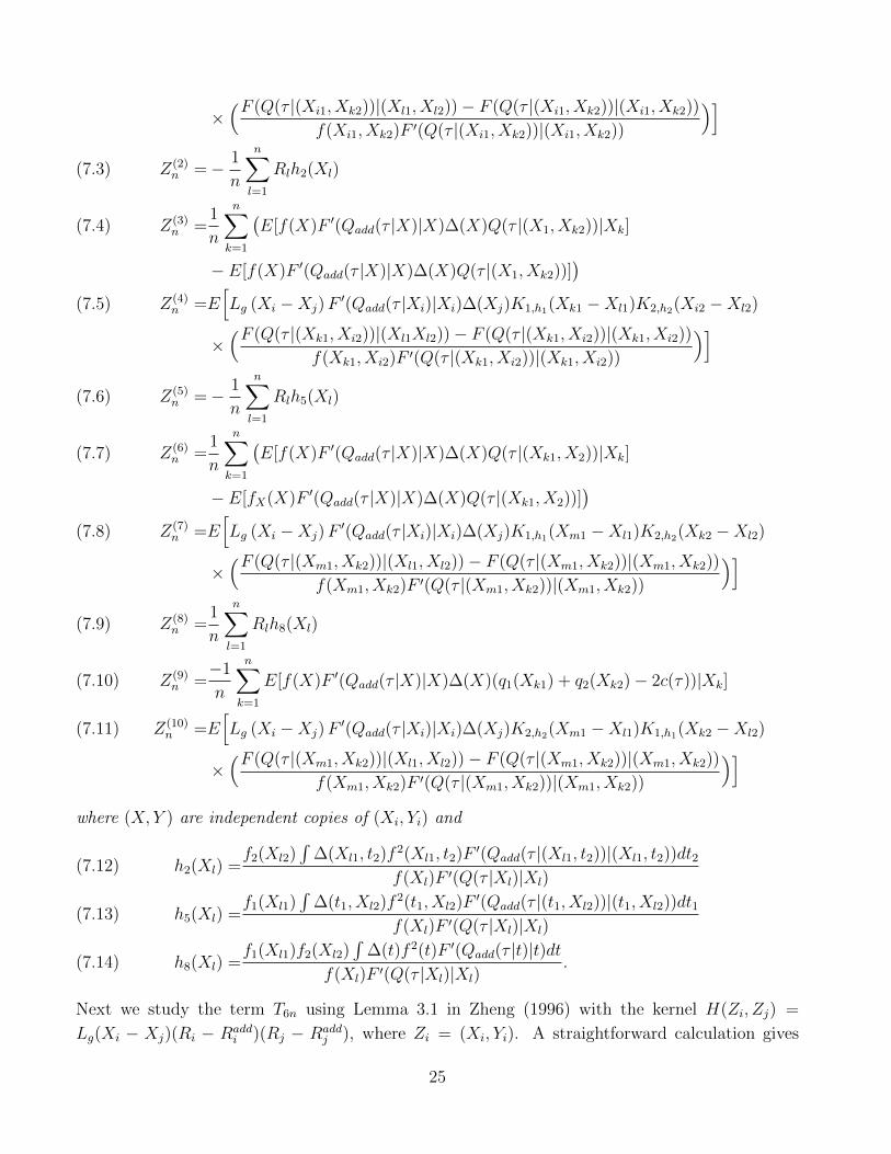
Lemma 7.1. Under the assumptions of Theorem 3.7 we have

(7.1) T5n =10∑j=1

Z(j)n + o

( 1√n

)in L1 where the terms Z

(j)n in this stochastic expansion are defined by

Z(1)n =E

[Lg (Xi −Xj)F

′(Qadd(τ |Xi)|Xi)∆(Xj)K1,h1(Xi1 −Xl1)K2,h2(Xk2 −Xl2)(7.2)

24

×(F (Q(τ |(Xi1, Xk2))|(Xl1, Xl2))− F (Q(τ |(Xi1, Xk2))|(Xi1, Xk2))

f(Xi1, Xk2)F ′(Q(τ |(Xi1, Xk2))|(Xi1, Xk2))

)]Z(2)n =− 1

n

n∑l=1

Rlh2(Xl)(7.3)

Z(3)n =

1

n

n∑k=1

(E[f(X)F ′(Qadd(τ |X)|X)∆(X)Q(τ |(X1, Xk2))|Xk](7.4)

− E[f(X)F ′(Qadd(τ |X)|X)∆(X)Q(τ |(X1, Xk2))])

Z(4)n =E

[Lg (Xi −Xj)F

′(Qadd(τ |Xi)|Xi)∆(Xj)K1,h1(Xk1 −Xl1)K2,h2(Xi2 −Xl2)(7.5)

×(F (Q(τ |(Xk1, Xi2))|(Xl1Xl2))− F (Q(τ |(Xk1, Xi2))|(Xk1, Xi2))

f(Xk1, Xi2)F ′(Q(τ |(Xk1, Xi2))|(Xk1, Xi2))

)]Z(5)n =− 1

n

n∑l=1

Rlh5(Xl)(7.6)

Z(6)n =

1

n

n∑k=1

(E[f(X)F ′(Qadd(τ |X)|X)∆(X)Q(τ |(Xk1, X2))|Xk](7.7)

− E[fX(X)F ′(Qadd(τ |X)|X)∆(X)Q(τ |(Xk1, X2))])

Z(7)n =E

[Lg (Xi −Xj)F

′(Qadd(τ |Xi)|Xi)∆(Xj)K1,h1(Xm1 −Xl1)K2,h2(Xk2 −Xl2)(7.8)

×(F (Q(τ |(Xm1, Xk2))|(Xl1, Xl2))− F (Q(τ |(Xm1, Xk2))|(Xm1, Xk2))

f(Xm1, Xk2)F ′(Q(τ |(Xm1, Xk2))|(Xm1, Xk2))

)]Z(8)n =

1

n

n∑l=1

Rlh8(Xl)(7.9)

Z(9)n =

−1

n

n∑k=1

E[f(X)F ′(Qadd(τ |X)|X)∆(X)(q1(Xk1) + q2(Xk2)− 2c(τ))|Xk](7.10)

Z(10)n =E

[Lg (Xi −Xj)F

′(Qadd(τ |Xi)|Xi)∆(Xj)K2,h2(Xm1 −Xl1)K1,h1(Xk2 −Xl2)(7.11)

×(F (Q(τ |(Xm1, Xk2))|(Xl1, Xl2))− F (Q(τ |(Xm1, Xk2))|(Xm1, Xk2))

f(Xm1, Xk2)F ′(Q(τ |(Xm1, Xk2))|(Xm1, Xk2))

)]where (X, Y ) are independent copies of (Xi, Yi) and

h2(Xl) =f2(Xl2)

∫∆(Xl1, t2)f

2(Xl1, t2)F′(Qadd(τ |(Xl1, t2))|(Xl1, t2))dt2

f(Xl)F ′(Q(τ |Xl)|Xl)(7.12)

h5(Xl) =f1(Xl1)

∫∆(t1, Xl2)f

2(t1, Xl2)F′(Qadd(τ |(t1, Xl2))|(t1, Xl2))dt1

f(Xl)F ′(Q(τ |Xl)|Xl)(7.13)

h8(Xl) =f1(Xl1)f2(Xl2)

∫∆(t)f 2(t)F ′(Qadd(τ |t)|t)dt

f(Xl)F ′(Q(τ |Xl)|Xl).(7.14)

Next we study the term T6n using Lemma 3.1 in Zheng (1996) with the kernel H(Zi, Zj) =

Lg(Xi − Xj)(Ri − Raddi )(Rj − Radd

j ), where Zi = (Xi, Yi). A straightforward calculation gives

25

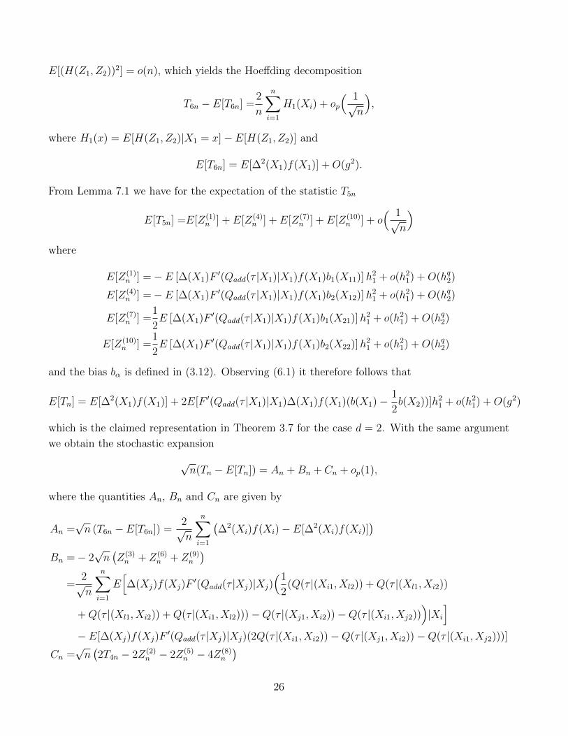
E[(H(Z1, Z2))2] = o(n), which yields the Hoeffding decomposition

T6n − E[T6n] =2

n

n∑i=1

H1(Xi) + op

( 1√n

),

where H1(x) = E[H(Z1, Z2)|X1 = x]− E[H(Z1, Z2)] and

E[T6n] = E[∆2(X1)f(X1)] +O(g2).

From Lemma 7.1 we have for the expectation of the statistic T5n

E[T5n] =E[Z(1)n ] + E[Z(4)

n ] + E[Z(7)n ] + E[Z(10)

n ] + o( 1√

n

)where

E[Z(1)n ] =− E [∆(X1)F

′(Qadd(τ |X1)|X1)f(X1)b1(X11)]h21 + o(h21) +O(hq2)

E[Z(4)n ] =− E [∆(X1)F


E[Z(7)n ] =

1

2E [∆(X1)F


E[Z(10)n ] =

1

2E [∆(X1)F


and the bias bα is defined in (3.12). Observing (6.1) it therefore follows that

E[Tn] = E[∆2(X1)f(X1)] + 2E[F ′(Qadd(τ |X1)|X1)∆(X1)f(X1)(b(X1)−1

2b(X2))]h

21 + o(h21) +O(g2)

which is the claimed representation in Theorem 3.7 for the case d = 2. With the same argument

we obtain the stochastic expansion

√n(Tn − E[Tn]) = An +Bn + Cn + op(1),

where the quantities An, Bn and Cn are given by

An =√n (T6n − E[T6n]) =

2√n

n∑i=1

(∆2(Xi)f(Xi)− E[∆2(Xi)f(Xi)]

)Bn =− 2

√n(Z(3)n + Z(6)

n + Z(9)n

)=

2√n

n∑i=1

E[∆(Xj)f(Xj)F

′(Qadd(τ |Xj)|Xj)(1

2(Q(τ |(Xi1, Xl2)) +Q(τ |(Xl1, Xi2))

+Q(τ |(Xl1, Xi2)) +Q(τ |(Xi1, Xl2)))−Q(τ |(Xj1, Xi2))−Q(τ |(Xi1, Xj2)))|Xi

]− E[∆(Xj)f(Xj)F

′(Qadd(τ |Xj)|Xj)(2Q(τ |(Xi1, Xi2))−Q(τ |(Xj1, Xi2))−Q(τ |(Xi1, Xj2)))]

Cn =√n(2T4n − 2Z(2)

n − 2Z(5)n − 4Z(8)

n

)26

=2√n

n∑i=1

Ri

(∆(Xi)f(Xi) + h2(Xi) + h5(Xi)− h8(Xi)

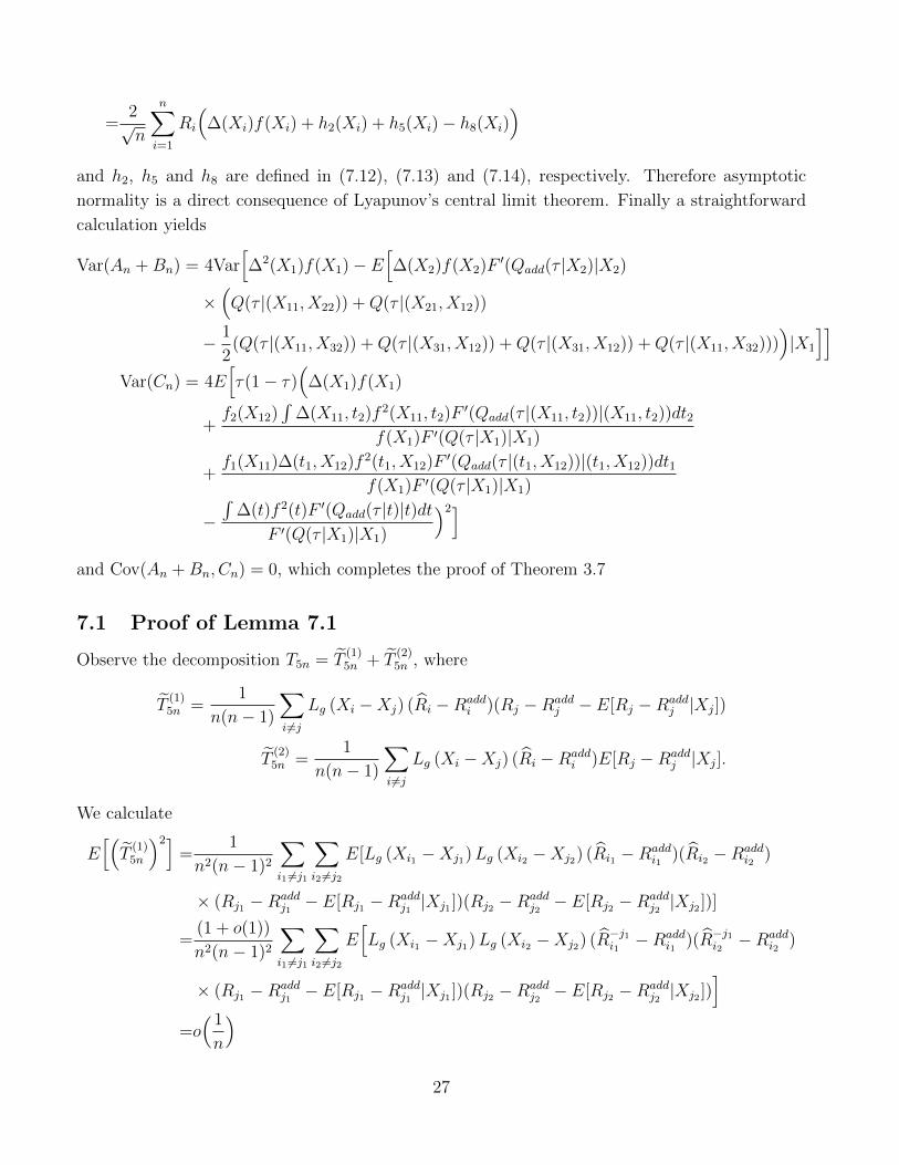
)and h2, h5 and h8 are defined in (7.12), (7.13) and (7.14), respectively. Therefore asymptotic

normality is a direct consequence of Lyapunov’s central limit theorem. Finally a straightforward

calculation yields

Var(An +Bn) = 4Var[∆2(X1)f(X1)− E

[∆(X2)f(X2)F

′(Qadd(τ |X2)|X2)

×(Q(τ |(X11, X22)) +Q(τ |(X21, X12))

− 1

2(Q(τ |(X11, X32)) +Q(τ |(X31, X12)) +Q(τ |(X31, X12)) +Q(τ |(X11, X32)))

)|X1

]]Var(Cn) = 4E

[τ(1− τ)

(∆(X1)f(X1)

+f2(X12)

∫∆(X11, t2)f

2(X11, t2)F′(Qadd(τ |(X11, t2))|(X11, t2))dt2

f(X1)F ′(Q(τ |X1)|X1)

+f1(X11)∆(t1, X12)f

2(t1, X12)F′(Qadd(τ |(t1, X12))|(t1, X12))dt1

f(X1)F ′(Q(τ |X1)|X1)

−∫

∆(t)f 2(t)F ′(Qadd(τ |t)|t)dtF ′(Q(τ |X1)|X1)

)2]and Cov(An +Bn, Cn) = 0, which completes the proof of Theorem 3.7

7.1 Proof of Lemma 7.1

Observe the decomposition T5n = T(1)5n + T

(2)5n , where

T(1)5n =

1

n(n− 1)

∑i 6=j


j − E[Rj −Raddj |Xj])

T(2)5n =

1

n(n− 1)

∑i 6=j

Lg (Xi −Xj) (Ri −Raddi )E[Rj −Radd

j |Xj].

We calculate

E[(T

(1)5n

)2]=

1

n2(n− 1)2

∑i1 6=j1

∑i2 6=j2

E[Lg (Xi1 −Xj1)Lg (Xi2 −Xj2) (Ri1 −Raddi1

)(Ri2 −Raddi2

)

× (Rj1 −Raddj1− E[Rj1 −Radd

j1|Xj1 ])(Rj2 −Radd

j2− E[Rj2 −Radd

j2|Xj2 ])]

=(1 + o(1))

n2(n− 1)2

∑i1 6=j1

∑i2 6=j2

E[Lg (Xi1 −Xj1)Lg (Xi2 −Xj2) (R−j1i1

−Raddi1

)(R−j1i2−Radd

i2)

× (Rj1 −Raddj1− E[Rj1 −Radd

j1|Xj1 ])(Rj2 −Radd

j2− E[Rj2 −Radd

j2|Xj2 ])

]=o( 1

n

)27

where the last estimate follows by similar arguments as given for the term T3n under the null

hypothesis [see Section 5]. With similar arguments we obtain

T(2)5n =

1

n(n− 1)

∑i 6=j

Lg (Xi −Xj) (F (Q−iadd(τ |Xi)|Xi)− F (Q(τ |Xi)|Xi))E[Rj −Raddj |Xj] + o

( 1√n

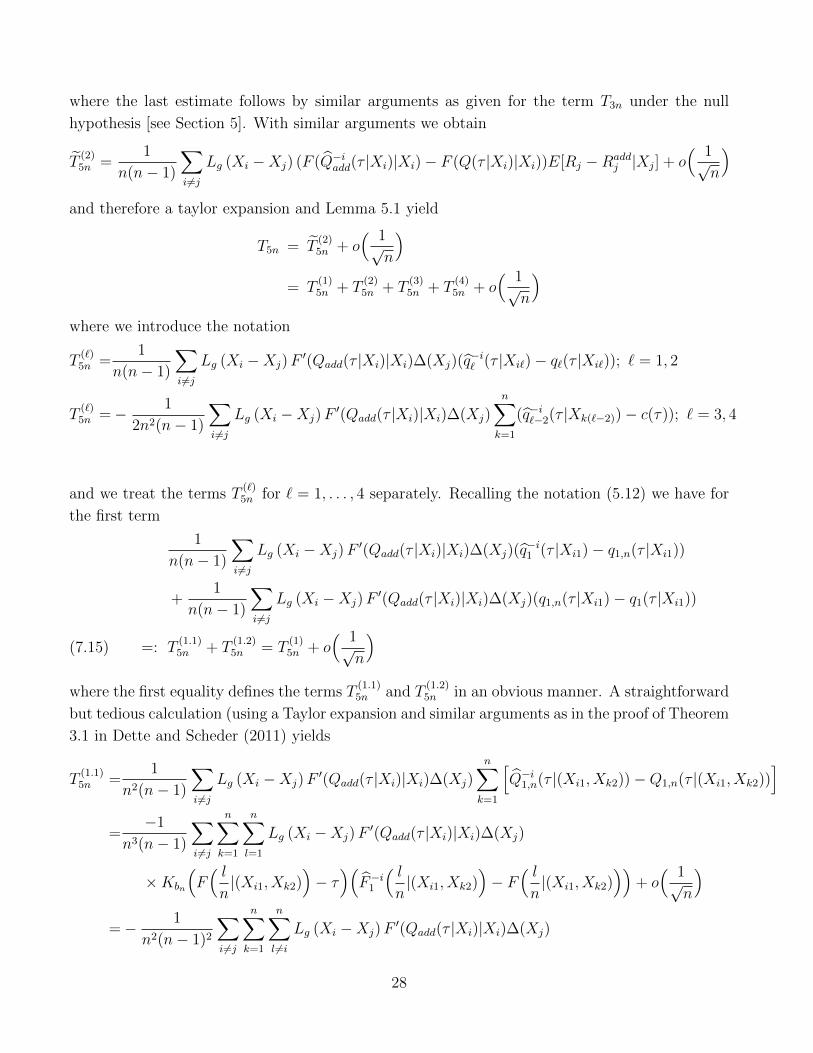
)and therefore a taylor expansion and Lemma 5.1 yield

T5n = T(2)5n + o

( 1√n

)= T

(1)5n + T

(2)5n + T

(3)5n + T

(4)5n + o

( 1√n

)where we introduce the notation

T(`)5n =

1

n(n− 1)

∑i 6=j

Lg (Xi −Xj)F′(Qadd(τ |Xi)|Xi)∆(Xj)(q

−i` (τ |Xi`)− q`(τ |Xi`)); ` = 1, 2

T(`)5n =− 1

2n2(n− 1)

∑i 6=j

Lg (Xi −Xj)F′(Qadd(τ |Xi)|Xi)∆(Xj)

n∑k=1

(q−i`−2(τ |Xk(`−2))− c(τ)); ` = 3, 4

and we treat the terms T(`)5n for ` = 1, . . . , 4 separately. Recalling the notation (5.12) we have for

the first term

1

n(n− 1)

∑i 6=j

Lg (Xi −Xj)F′(Qadd(τ |Xi)|Xi)∆(Xj)(q

−i1 (τ |Xi1)− q1,n(τ |Xi1))

+1

n(n− 1)

∑i 6=j

Lg (Xi −Xj)F′(Qadd(τ |Xi)|Xi)∆(Xj)(q1,n(τ |Xi1)− q1(τ |Xi1))

=: T(1.1)5n + T

(1.2)5n = T

(1)5n + o

( 1√n

)(7.15)

where the first equality defines the terms T(1.1)5n and T

(1.2)5n in an obvious manner. A straightforward

but tedious calculation (using a Taylor expansion and similar arguments as in the proof of Theorem

3.1 in Dette and Scheder (2011) yields

T(1.1)5n =

1

n2(n− 1)

∑i 6=j


n∑k=1

[Q−i1,n(τ |(Xi1, Xk2))−Q1,n(τ |(Xi1, Xk2))

]=

−1

n3(n− 1)

∑i 6=j

n∑k=1

n∑l=1


×Kbn

(F( ln|(Xi1, Xk2)

)− τ)(F−i1

( ln|(Xi1, Xk2)

)− F

( ln|(Xi1, Xk2)

))+ o( 1√

n

)=− 1

n2(n− 1)2

∑i 6=j

n∑k=1

n∑l 6=i


28

×∫ 1

0

Kbn (F (t|(Xi1, Xk2))− τ)K1,h1(Xi1 −Xl1)K2,h2(Xk2 −Xl2)

× IYl ≤ t − F (t|(Xi1, Xk2))

f(Xi1, Xk2)dt+ o

( 1√n

)= Z(1)

n + Z(2)n + o

( 1√n

)where Z

(1)n is defined in (7.2) and

Z(2)n =

−1

n3(n− 1)

∑i 6=j

n∑k=1

n∑l 6=i


×∫ 1

0

Kbn (F (t|(Xi1, Xk2))− τ)K1,h1(Xi1 −Xl1)K2,h2(Xk2 −Xl2)s(t|Xl)εlf(Xi1, Xk2)

dt

=Z(2)n + o

( 1√n

).

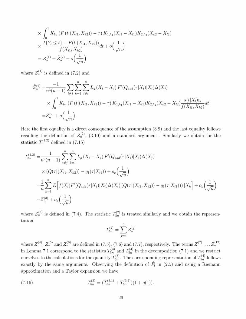
Here the first equality is a direct consequence of the assumption (3.9) and the last equality follows

recalling the definition of Z(2)n , (3.10) and a standard argument. Similarly we obtain for the

statistic T(1.2)n defined in (7.15)

T(1.2)5n =

1

n2(n− 1)

n∑i 6=j

n∑k=1


× (Q(τ |(Xi1, Xk2))− q1(τ |Xi1)) + op

( 1√n

)=

1

n

n∑k=1

E[f(Xi)F

′(Qadd(τ |Xi)|Xi)∆(Xi) (Q(τ |(Xi1, Xk2))− q1(τ |Xi1))) |Xk

]+ op

( 1√n

)=Z(3)

n + op

( 1√n

)where Z

(3)n is defined in (7.4). The statistic T

(2)5n is treated similarly and we obtain the represen-

tation

T(2)5n =

6∑j=4

Z(j)n

where Z(4)n , Z

(5)n and Z

(6)n are defined in (7.5), (7.6) and (7.7), respectively. The terms Z

(7)n , . . . Z

(12)n

in Lemma 7.1 correspond to the statistics T(3)5n and T

(4)5n in the decomposition (7.1) and we restrict

ourselves to the calculations for the quantity T(3)5n . The corresponding representation of T

(4)5n follows

exactly by the same arguments. Observing the definition of Fl in (2.5) and using a Riemann

approximation and a Taylor expansion we have

(7.16) T(3)5n = (T

(3.1)5n + T

(3.2)5n )(1 + o(1)).

29

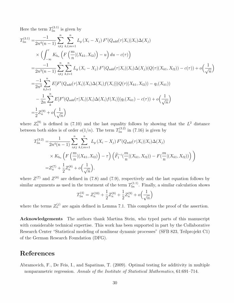
Here the term T(3.1)5n is given by

T(3.1)5n =

−1

2n4(n− 1)

n∑i 6=j

n∑k,l,m=1


×(∫ τ

−∞Kbn

(F(mn|(Xk1, Xl2)

)− u)du− c(τ)

)=

−1

2n3(n− 1)

n∑i 6=j

n∑k,l=1

Lg (Xi −Xj)F′(Qadd(τ |Xi)|Xi)∆(Xj)(Q(τ |(Xk1, Xl2))− c(τ)) + o

( 1√n

)=−1

2n2

n∑k,l=1

E[F ′(Qadd(τ |Xi)|Xi)∆(Xi)f(Xi)](Q(τ |(Xk1, Xl2))− q1(Xk1))

− 1

2n

n∑k

E[F ′(Qadd(τ |Xi)|Xi)∆(Xi)f(Xi)](q1(Xk1)− c(τ)) + o( 1√

n

)=

1

2Z(9)n + o

( 1√n

)where Z

(9)n is defined in (7.10) and the last equality follows by showing that the L2 distance

between both sides is of order o(1/n). The term T(3.2)5n in (7.16) is given by

T(3.2)5n =

1

2n4(n− 1)

n∑i 6=j

n∑k,l,m=1


×Kbn

(F(mn|(Xk1, Xl2)

)− τ)(

F−i1 (m

n|(Xk1, Xl2))− F (

m

n|(Xk1, Xl2))

))=Z(7)

n +1

2Z(8)n + o

( 1√n

),

where Z(7) and Z(8) are defined in (7.8) and (7.9), respectively and the last equation follows by

similar arguments as used in the treatment of the term T(1.1)5n . Finally, a similar calculation shows

T(4)5n = Z(10)

n +1

2Z(8)n +

1

2Z(9)n + o

( 1√n

)where the terms Z

(j)n are again defined in Lemma 7.1. This completes the proof of the assertion.

Acknowledgements The authors thank Martina Stein, who typed parts of this manuscript

with considerable technical expertise. This work has been supported in part by the Collaborative

Research Center “Statistical modeling of nonlinear dynamic processes” (SFB 823, Teilprojekt C1)

of the German Research Foundation (DFG).

References

Abramovich, F., De Feis, I., and Sapatinas, T. (2009). Optimal testing for additivity in multiple

nonparametric regression. Annals of the Institute of Statistical Mathematics, 61:691–714.

30

Carroll, R. J., Hardle, W., and Mammen, E. (2002). Estimation in an additive model when the

parameters are linked parametrically. Econometric Theory, 18(4):886–912.

Chernozhukov, V., Fernandez-Val, I., and Galichon, A. (2010). Quantile and probability curves

without crossing. Econometrica, 78(3):1093–1125.

De Gooijer, J. G. and Zerom, D. (2003). On additive conditional quantiles with high-dimensional

covariates. Journal of the American Statistical Association, 98(461):135–146.

Derbort, S., Dette, H., and Munk, A. (2002). A test for additivity in nonparametric regression.

Annals of the Institute of Statistical Mathematics, 54:60–82.

Dette, H., Neumeyer, N., and Pilz, K. F. (2006). A simple nonparametric estimator of a strictly

monotone regression function. Bernoulli, 12:469–490.

Dette, H. and Scheder, R. (2010). A finite sample comparison of nonparametric estimates of the

effective dose in quantal bioassay. Journal of Statistical Computation and Simulation, 80(5):527–

544.

Dette, H. and Scheder, R. (2011). Estimation of additive quantile regression. Annals of the

Institute of Statistical Mathematics, 63(2):245–265.

Dette, H. and Volgushev, S. (2008). Non-crossing nonparametric estimates of quantile curves.

Journal of the Royal Statistical Society, Ser. B, 70(3):609–627.

Dette, H. and von Lieres und Wilkau, C. (2001). Testing additivity by kernel-based methods -

what is a reasonable test? Bernoulli, 7:669–697.

Doksum, K. and Koo, J. Y. (2000). On spline estimators and prediction intervals in nonparametric

regression. Computational Statistics and Data Analysis, 35:67–82.

Eubank, R. L., Hart, J. D., Simpson, D. G., and Stefanski, L. A. (1995). Testing for additivity in

nonparametric regression. Annals of Statistics, 23(6):1896–1920.

Fan, Y. and Linton, O. (2003). Some higher-order theory for a consistent non-parametric model

specification test. Journal of Statistical Planning and Inference, 109(1-2):125–154.

Gozalo, P. L. and Linton, O. B. (2001). Testing additivity in generalized nonparametric regression

models with estimated parameters. Journal of Econometrics, 104(1):1–48.

Hall, P. (1984). Central limit theorem for integrated square error of multivariate nonparametric

density estimators. Journal of Multivariate Analysis, 14:1–16.

Hall, P., Wolff, R. C. L., and Yao, Q. (1999). Methods for estimating a conditional distribution

function. Journal of the American Statistical Association, 94(445):154–163.

31

Hardle, W., Jeong, K., and Song, R. (2012). A consistent nonparametric test for causality in

quantile. Econometric Theory, to appear.

Hengartner, N. W. and Sperlich, S. (2005). Rate optimal estimation with the integration method

in the presence of many covariates. Journal of Multivariate Analysis, 95(2):246–272.

Horowitz, J. and Lee, S. (2005). Nonparametric estimation of an additive quantile regression

model. Journal of the American Statistical Association, 100(472):1238–1249.

Koenker, R. (2005). Quantile Regression. Cambrige University Press, New York.

Koenker, R. and Bassett, G. (1978). Regression quantiles. Econometrica, 46(1):33–50.

Lee, Y. K., Mammen, E., and U., P. B. (2010). Backfitting and smooth backfitting for additive

quantile models. Annals of Statistics, 38(5):2857–2883.

Linton, O. B. and Nielsen, J. P. (1995). A kernel method of estimating structured nonparametric

regression based on marginal integration. Biometrika, 82(1):93–100.

Mammen, E., Linton, O. B., and Nielsen, J. (1999). The existence and asymptotic properties of a

backfitting projection algorithm under weak conditions. Annals of Statistics, 27(5):1443–1490.

Nielsen, J. P. and Sperlich, S. (2005). Smooth backfitting in practice. Journal of the Royal

Statistical Society, Ser. B, 67(1):43–61.

Nolan, D. and Pollard, D. (1987). U-processes: rates of convergence. The Annals of Statistics,

15(2):780–799.

Sun, Y. (2006). A consistent nonparametric equality test of conditional quantile functions. Econo-

metric Theory, 22:614–632.

van der Vaart, A. W. and Wellner, J. A. (1996). Weak Convergence and Empirical Processes.

Springer Series in Statistics. Springer, New York.

Yu, K. and Jones, M. C. (1997). A comparison of local constant and local linear regression quantile

estimators. Computational Statistics and Data Analysis, 25(2):159–166.

Yu, K. and Jones, M. C. (1998). Local linear quantile regression. Journal of the American

Statistical Association, 93(441):228–237.

Zhang, C. and Dette, H. (2004). A power comparison between nonparametric regression tests.

Statistics and Probability Letters, 66:289–301.

Zheng, J. X. (1996). A consistent test of a functional form via nonparametric estimation tech-

niques. Journal of Econometrics, 75:263–289.

32

Documents

Testing for additivity in nonparametric quantile regression · 2015-08-20 · Testing for additivity in nonparametric quantile regression Holger Dette, Matthias Guhlich Ruhr-Universit