Testing Behavioral Finance Theories Using Trends and Sequences in Financial Performance

Wesley S. Chan wschan@mit.edu, (617) 253-3919

Richard Frankel

frankel@mit.edu, (617) 253-7084

and

S. P. Kothari kothari@mit.edu, (617) 253-0994

Sloan School of Management Massachusetts Institute of Technology

50 Memorial Drive, E52-325 Cambridge, MA 02142

April 18, 2001 Current Draft: July 2002

Abstract

Models based on psychological biases can explain momentum and reversal in stock returns, but risk overfitting of theory to data. We examine a central psychological bias, representativeness, which underlies many behavioral-finance theories. According to this bias, individuals form predictions about future outcomes based on how closely past outcomes fit certain categories. To produce out-of sample tests, we use accounting performance to identify these categories and test the idea that investors misclassify firms and thus make biased forecasts. We find evidence of short-term accounting momentum, consistent with the idea that investors fail to immediately incorporate new information, but find no support for long-term reversal related to accounting performance. Contrary to theory, we find little evidence that the consistency of past accounting performance is related to future returns.

Trends and Sequences in Financial Performance: A Test of Behavioral Theories

I. Introduction

Several papers document momentum in stock returns at horizons ranging from three to

twelve months and reversals at longer horizons (e.g., Jegadeesh and Titman, 1993 and 2001, and

DeBondt and Thaler, 1985 and 1987). This predictability of returns, particularly at long

horizons, has been widely debated (e.g., Fama, 1998), although the notion that it indicates market

inefficiency is rapidly gaining currency (e.g., Shleifer, 2000). Recently, many have attempted to

add rigor to the inefficient markets hypothesis by developing theories based on investors’ biased

information processing.1 Almost invariably, the human information processing bias that

underlies a given model of market inefficiency is a variation of the representativeness hueristic.

Indeed surveys of the literature on biases in human information processing and behavioral

finance suggest the centrality of representativeness to theories of systematic mispricing (see

Daniel, Hirshleifer, and Teoh, 2002, and our discussion in section 2 of the paper). In behavioral

finance models and empirical work, the pattern of past performance is an important driver of

representativeness. We argue that patterns, i.e., trends and sequences, in financial performance

operationalize representativeness. Accordingly, we use a previously unexplored context (i.e.,

patterns in financial performance) to construct out-of-sample tests of behavioral theories that

predict systematic mispricing.

Assessing the predictive ability of behavioral hypotheses using out-of-sample data is

important (see Fama, 1998, Hong and Stein, 1999, and Barberis et al., 1998). Absent such tests,

the potentially boundless set of psychological biases that theorists can use to build behavioral

models and explain observed phenomena creates the potential for ‘theory dredging.’2 Thus, by

1 Some of the notable attempts to construct formal behavioral theories include Barberis, Shleifer, and Vishny (1998), Daniel, Hirschleifer, and Subramanyam (1998), Hong and Stein (1999), and Mullainathan (2001). 2 See Rubinstein (2001), Hirshliefer (2001), and Shiller (1999). Fama (1991) uses the term ‘theory dredging’ to describe the practice for overfitting theories to empirical observation.

2

identifying pervasive psychological biases, forming empirically rejectable hypotheses, and

testing for their validity, we can aid behavioral theorists in isolating the fundamental behavioral

phenomena, if any, that influence asset pricing. Miller (1986) surmises, “That we abstract from

all these stories in building our models is not because the stories are uninteresting but because

they may be too interesting and thereby distract us from the pervasive market forces that should

be our principal concern.” In this spirit, we distill behavioral underpinnings of the theories and

test for the predicted systematic mispricing.

Summary of findings. We examine the relation between past trends and sequences in

financial performance and future returns. We fail to find evidence that investors systematically

over-extrapolate a consistent sequence of financial performance at long horizons. Abnormal

returns in the year after five years of high or low growth are statistically and economically

insignificant. We find some evidence that investors underreact to a one-year trend in accounting

performance, but this phenomenon does not appear to be distinct from post-earnings

announcement drift. In addition, the consistency or pattern of firm performance does not

incrementally influence expectations. Finally, the past trend and pattern of growth do not lead to

predictable returns following subsequent performance that confirms or contradicts this past trend.

Thus, our evidence fails to suggest that patterns or trends in past financial growth rates lead

investors to form biased expectations about future firm performance. These results present a

challenge to the entire class of representativeness-based theories. While investors may form

biased expectations about future firm growth rates using information outside of accounting

statements, to date behavioral theories have not made this distinction.

Caveats. An important maintained hypothesis underlying behavioral theories of

mispricing is that arbitrage is limited and thus it cannot eliminate the mispricing completely (see

De Long et al., 1990, Shleifer and Vishny, 1997, and Barberis, Shleifer, and Vishny, 1998).

Thus, failure to find evidence of mispricing consistent with behavioral theories is not necessarily

3

a strike against the model because the maintained hypothesis of limited arbitrage might not be

descriptive. Future research might attempt to test the predictions in markets that a priori exhibit

variation with respect to the descriptive validity of the maintained hypothesis of limited

arbitrage.

Outline of the paper. Section II discusses the representativeness bias, develops

hypotheses about the stock price consequences of the bias based on the behavioral finance

models, and states the predictions. Section III describes the data and the test methodology.

Section IV discusses results, and section V concludes.

II. Hypotheses development

In section 2.1 we discuss the representativeness bias and its role in the formation of

investor expectations. The discussion seeks to establish that representativeness bias is perhaps

the most prominent in the literature on human information processing and that it underlies many

behavioral finance theories. Section 2.2 describes how we operationalize representativeness bias

in order to conduct empirical tests. Section 2.3 presents our predictions about security return

behavior when investors’ expectations are biased due to representativeness.

2.1 Representativeness bias

Individuals are thought to make biased judgements under uncertainty because limited

time and cognitive resources lead them to apply heuristics like representativeness (Hirshleifer,

2001). Representativeness is the tendency of individuals to classify things into discrete groups

based on similar characteristics. Tversky and Kahneman (1974) note that because individuals

focus on similarities, they diverge from rational reasoning in many ways. First, subjects fail to

consider base rates. For example, they may think a rock is gold because of its salient

characteristics like color and weight and in so doing fail to consider the low probability of

finding gold. Second, subjects fail to incorporate sample size or the precision of qualitative

information in their classifications and predictions. Therefore, they can confidently believe two

companies have significantly different financial prospects despite a limited sample of prior

performance. Finally, in their desire to maintain distinct categories, subjects making predictions

4

fail to realize extreme observations are unlikely to be repeated. Thus, after a history of

outstanding performance, investors are disappointed when future performance regresses to the

mean. In sum, representativeness implies sequences of past performance cause investors to place

a firm into a category, and form predictably biased expectations about future performance.

The centrality of the representativeness heuristic to behavioral theory can be seen from

the number of specific biases that exemplify its logic. For example, in the “halo effect,”

individuals observing a positive characteristic of a firm form expectations about other

characteristics. The “clustering illusion” and the “hot hand” misconceptions predict that

investors seeing a sequence of repeated returns incorrectly characterize them as following a

trend. Consistent with this bias, Sirri and Tufano (1998) find increased flows into mutual funds

with exceptional (but statistically short-lived) past performance. Lakonishok, Shleifer, and

Vishny (1994) cite the base rate bias and investors’ tendency to make categorical predictions to

explain the profitability of contrarian investment strategies.3

The representativeness bias also underlies many recent models in behavioral finance.

While each author uses somewhat different assumptions and approaches in developing their

model, they all assume some investor irrationality that is consistent with representativeness. For

example, Barberis et al. (1998) assume investors always infer an incorrect earnings process on

the basis of recent evidence. A string of good earnings announcements inclines the investors to

incorrectly conclude a trending performance and thus causes an excessive stock price increase.

Mullainathan (2001) assumes that individuals are not Bayesian because they think in discrete

categories and thus assume the most representative scenario, ignoring (i.e., underweighting)

plausible alternative states of the world. Hong and Stein (1999) assume heterogeneous groups of

investors with each group utilizing only a subset of the information. One group, the

3 For a more extensive exposition and discussion of the predictable errors in judgment related to categorical thinking, see Mullainathan (2001) and Rabin (2001). Mullainathan incorporates investors who shift their beliefs abruptly from one category to another when changing their mind, instead of gradually updating probabilities in response to new information as in Barberis et al. (1998).

5

“newswatchers,” underreacts (i.e., is not Bayesian) to new information. The other group,

momentum traders, extrapolates past sequences of price changes and thus corrects for the

newswatchers’ underreaction, but the process ultimately leads to an overreaction. In the Daniel,

Hirschleifer, Subramanyam (1998) set up, a string of good news leads to overreaction because

the public announcements of good news cause investors to be increasingly overconfident of their

private information. That is, a sequence of good news announcements is thought to be

representative of trending expectations and this leads to overpriced stocks. In summary, either

because investors assume the wrong model or because they are not Bayesians, investors form

expectations that are influenced by strings, sequences, or patterns of financial performance and

thus suffer from some form of representativeness bias.

2.2 Operationalizing representativeness

To operationalize the representativeness bias, we focus on trends and sequences of

financial performance. In this respect, Tversky and Kahneman (1974, p. 1125) note that

consistency of past data affects the formation of categories because “People expect that a

sequence of events generated by a random process will represent the essential characteristics of

that process even when the sequence is short.” Thus, we examine whether the consistency of

past financial performance in the subperiods that comprise the overall trend predicts future

returns. Moreover, whereas past models generally focus on earnings performance, we believe the

models are intended to be general. Indeed, Barberis et al. (1998, p. 308) predict that “…

securities with strings of good performance, however measured, receive extremely high

valuations, and these valuations, on average, return to the mean” (emphasis added).

Additional reasons suggest financial performance measures are a credible means of

testing the behavioral theories. “Salience” and “availability” of information are central to

subjects’ representativeness bias and expectation formation (see Tversky and Kahneman, 1974).

Financial performance measures are both salient and easily available to a broad cross-section of

investors. The recent catastrophic reactions to financial reports and disclosures underscore the

salience of accounting information in the capital markets. However, because theory does not

6

suggest which measure of financial performance is most ‘salient’ to investors, we employ growth

rates in three measures: sales, net income, and operating income.

2.3 Predictions

Representativeness can lead investors to incorrectly extrapolate existing trends (Daniel,

Hirshleifer, and Teoh, 2002) and cause overreaction, which reverses at a later date once incorrect

conclusions are proven false. This prediction entails the following three steps that also underlie

previous research (e.g., Bernard and Thomas, 1990, Dechow and Sloan, 1997, and Daniel and

Titman, 2002). First, researchers define a model of biased investor expectations about dividends.

Second, researchers specify a model of how dividends truly evolve. Third, researchers derive the

pattern of errors in expectations, which can predict patterns of stock returns.

With respect to investors’ biased expectations, extant behavioral models do not specify

the length of the past performance window necessary to generate overly optimistic or pessimistic

dividend expectations. For example, the interval could be the prior four quarters, five years, or

something else. At the risk of data dredging, we experiment with long-term (five years) and

medium-term (one year of quarterly) financial performance intervals in part because predictions

about returns following medium-term performance are ambiguous. The empirical findings on

momentum by Jegadeesh and Titman (1993) and others suggest that underreaction to information

occurs. Accordingly, some behavioral finance theories incorporate investor belief in a mean-

reverting category, as in Barberis et al. (1998).4 Investors that believe a sequence comes from a

mean-reverting process will be likely to discount the possibility of trends. However, it is

theoretically possible that investors could believe in a trending category at this horizon.

Therefore, strictly speaking representativeness could predict either drift or reversal in the

medium term. In contrast, the consensus among behavioral theorists appears to be that extreme

financial performance over a five-year horizon would clearly lead to over-optimism or undue

4 This model also leads to overreaction, as the trending performance observations accumulate over a long horizon, investors confidently reclassify the firm to a trending category and thus form over-optimistic or pessimistic expectations.

7

pessimism, and subsequent price reversals. The trend over a longer horizon makes it more likely

that investors will place it into a trending category.

Representativeness bias also suggests that the consistency of performance in the

subintervals that comprise the performance interval (i.e., four quarters or five years) influences

investor optimism or pessimism. A consistent performance pattern should be more salient and

thus lead to more definitive classification by investors. Thus, we examine whether consistent

financial performance over one- and five-year horizons leads to price over-reaction and

subsequent reversals.

We also examine price performance following a confirming or disconfirming

announcement at the end of a string of consistent financial performance announcements. Price

performance following confirming and disconfirming announcements sheds light on whether

investors suffering from a representativeness bias initially overreact, but then de-emphasize an

observation that confirms their bias, or correct for the past overreaction when faced with a

disconfirming observation. Therefore, we test whether the magnitude and consistency of

accounting performance in the prior four quarters or five years generates return momentum

following confirming observations and reversal following disconfirming observations.

Specifically, based on the representativeness heuristic, we predict that investors use the

sequence of past quarterly or annual growth rates to place a firm into one of three categories:

1) Perceived high growth firms. These firms have the highest past growth rates and most consistently positive quarterly (annual) results relative to their peers. Investors expect firms in this category to continue growing, and thus overvalue them.

2) Perceived distressed/low growth firms. These firms experience a sequence of steadily

falling (and possibly negative) growth. Investors expect firms in this category to continue to display unfavorable relative performance and thus undervalue them.

3) Perceived non-trending firms.5 These firms exhibit a cyclical pattern of growth.

Investors likely believe that these firms’ performance will revert in the near term. They may therefore underweight recent public signals and cause momentum in returns.

5 This category includes the “mean-reverting” regime featured in the model of Barberis et al. (1998). We choose to classify firms into “non-trending” because 1) it is not clear that we have enough data to define operating results as

8

The high growth and distressed categories resemble the growth and value dichotomy that

has received much attention in research and the financial press. Because investor expectations of

earnings for the high (low) growth firms are too optimistic (pessimistic) and valuation too high

(low), the high (low) growth firms are expected to underperform (outperform) the market. While

previous research (see, for example, Lakonishok, Shleifer, and Vishny, 1994, and La Porta,

Lakonishok, Shleifer, and Vishny, 1997) makes a similar prediction assuming that investors

extrapolate growth. However, in our analysis, the overall trend and the sequence in performance

are important. That is, an additional prediction based on representativeness bias is that firms

with a consistent prior performance pattern should experience greater reversals.

Performance measurement horizon is also likely to affect the strength of the subsequent

price performance for the high and low growth category firms. Based on previous evidence of

medium-term momentum (Jegadeesh and Titman, 1993) and some evidence of long-term

reversals (see DeBondt and Thaler, 1985 and 1987, and Ball, Kothari, and Shanken, 1995), we

expect the high and low growth firms to exhibit bigger price reversals when assigned to those

categories on the basis of consistency of five-year performance than four-quarter performance.

Returns are expected to exhibit momentum if they fall into the third, non-trending growth

category. In this case, investors seeing the beginnings of a trend will discount it and hold even

more strongly to a belief that performance will revert. As they are surprised by the trending

results, a drift in returns develops. Barberis et al. (1998) and Rabin (2001) rely on this form of

bias to generate momentum. Thus, the behavioral explanation for momentum is that investors

underreact to information, delaying its incorporation into prices and leading to return

predictability. Because information comes from a variety of sources, our tests of financial

performance can be viewed as an attempt to isolate the particular type of information that

investors are slow to assimilate. Cohen, Gompers, Vuolteenaho (2001) argue that investors

truly mean-reverting, and 2) some theories, e.g. Mullainathan (2001), feature broader non-trending categories of investor belief.

9

underreact to information about cash flows, or the part of the return that predicts future financial

performance. A related but simpler idea is that investors underreact to past financial

performance, as opposed to information about growth prospects. Daniel and Titman (2001)

provide evidence that the latter is important to investor misperception. Under this framework,

investors do not fully digest financial performance, and so financial growth forecasts returns in

the same direction over the next several months. Thus, as mentioned above, investors are more

likely to underreact if they classify firms into a non-trending (or even mean-reverting) category.

III. Variable measurement, tests, and data

In the first part of this section we discuss the rationale for examining various

performance measures, long- and medium- horizon prior returns, and the consistency of prior

performance. We do so by relating these research design choices to the representativeness bias.

The second part of this section, details the implementation of these choices.

3.1 Performance measures

Below we describe the performance measures used in the tests and define the trend and

consistency of performance. We calculate financial growth rates over two periods: one year

(four rolling quarters) and five years (using annual data). For each we use three accounting

measures of performance: sales, net income, and operating income. One drawback of sales per

share is that it may have little relation to underlying profitability and this relation may vary

across firms and industries. Therefore, if investors focus on profitability, sales will not measure

the variation in financial performance that they perceive to be a key driver of future dividends.

The remaining two financial performance measures are change in net income per share, NI, and

operating income, OI, scaled by base period assets per share, A. Using assets in the denominator

enables computation of a performance measure in periods where net income is negative. Simple

earnings-per-share growth measures would not be meaningful in these contexts. The third

measure utilizes operating income after depreciation-per-share instead of net income-per-share

because large one-time items can affect the net income measure of financial performance.

10

Specifically, we select all firms each calendar period with data on the specified measure

of financial growth. For tests based on medium-term horizon, we use all firms in the Compustat

quarterly database from 1976-2000 with at least seven past quarters of data.6 Returns for each

firm-quarter observation are computed after the end of each March, June, September, and

December and financial performance is computed based on data from the previous calendar

quarter. The one-quarter lag ensures that financial data are publicly available prior to return

computation. Our financial performance measures are based upon the trend of past growth from

one year to the next, where year is defined as a non-overlapping four-quarter period. To be

precise, quarterly financial performance is computed as

[(St + S t-1 + St-2 + St-3) - (St-4+ St-5 + S t-6 + S t-7)]/(S t-4+ S t-5 + S t-6 + S t-7)

for the sales-per-share measure, and

(NI t + NI t-1 + NI t-2 + NI t-3) - (NI t-4+ NI t-5 + NI t-6 + NI t-7)/A t-4

for the net income measure. At-4 represents assets four calendar quarters before the current

quarter t. A similar method is used to compute the operating income measure. While the growth

measures would be identical to those obtained by replacing the sum of four quarterly figures with

an annual figure, we use the quarterly figures because: (i) we calculate growth rates every

quarter; and (ii) we define consistency in growth on the basis of the pattern of four quarterly

seasonal growth rates within a year.

For the long-horizon growth rates, each year from 1975 to 1999 we select all firms with at

least five years of past data on the Compustat Annual data file.7 Each year we assume that

annual financial data are available by the end of June for fiscal years ending in any of the months

of the preceding calendar year and thus perform return analysis using price data starting on July

1. Five-year sales growth is calculated using annual sales numbers as:

6 This requirement provides the data necessary for the consistency tests discussed below. To control for seasonality of performance, we calculate growth relative to year-ago numbers each quarter.

11

(St – St-5)/St-5

and five-year growth in annual net income is

(NIt – NIt-5)/At-5

and operating income growth is defined by replacing NI with OI.

Trend, consistency, and confirming or disconfirming growth. Below we describe our

classification on the basis of trend and consistency of growth they experience over previous four

quarters or five years. Unless stated otherwise, the description applies to performance measures

for both one and five years.

Trend. Each quarter (year) we rank firms on the basis of each performance measure.

Firms in the top quintile by growth are labeled “high growth” firms, and those in the bottom

quintile are “low growth” firms. Since the assignment of stocks to the growth quintiles is based

only on the growth over the entire horizon, i.e., one or five years, it is a measure of trend.

Consistency. To test for the effects related to consistency of past performance, we rank

firms within each performance quintile by consistency of performance in the sub intervals that

comprise the performance metric. For the one-year (five-year) sample, we examine performance

in each of the four quarters (five years). Consistency ranks for a given firm are determined by

the number of quarters (years) in which that firm experiences above median seasonal quarterly

(year-on-year) growth relative to the entire cross section of firms available in that quarter (year).

Those top growth quintile firms with above median growth in all four quarters (five years) within

the past one-year (five-year) period are labeled “consistent” growers. Those top quintile firms

with only two-or-fewer quarters (three-or-fewer years) of above median growth are called

“inconsistent” growers. We repeat the process for bottom quintile firms, so that firms with four

quarters (five years) of below median growth are “consistent” and firms with two-or-fewer

quarters (three-or-fewer years) of below median growth are “inconsistent.” We choose to use

7 We select this date range to match the quarterly sample period. Note that we require firms to have five years of past data. This sample period reduces survivor bias resulting from Standard and Poors’s incorporation of back-filled data on existing NASDAQ stocks in the mid-seventies.

12

only three consistency categories to ensure adequate observations in each portfolio. Changing

the number of periods used to define a consistency category does not alter the tenor of the results.

Confirming or contradictory growth observation. Another way to determine if

consistency, i.e., the past pattern of growth affects investor expectations is to examine investors’

reaction when a firm’s recent performance contradicts past performance. For example, consistent

high growth firms with a subsequent low growth quarter will disappoint investors, but these

investors may be slower to assimilate information that contradicts a prior categorization. In

contrast, investors should be less resistant to new information on firms that are inconsistent.

Similarly, consistent firms should experience less drift after an additional quarter of confirming

growth, while inconsistent firms should experience more as investors slowly revise their

expectations to include the possibility of a trend.

3.2 Tests of price performance

Price performance following growth trends. To test whether investors react to financial

performance according to the behavioral theories, we construct a trading strategy that involves

buying and selling equal-weight portfolios of high- and low-growth firms, respectively. We hold

these portfolios without rebalancing for three, six, nine, and 12-month horizons and refer to

returns produced by this strategy as “long-short” returns.

Medium-term horizon. As discussed earlier, over medium-term horizons, both over- and

under-reaction are possibilities (depending on the behavioral theory assumed). Positive profits

for the long-short strategy would imply that investors do not rationally and fully adjust to

information contained in publicly available accounting statements, and therefore returns continue

to drift in the same direction as past financial growth. This is the “accounting momentum”

effect. Alternatively, if a one-year growth trend were sufficient for investors to extrapolate into

the future and cause an over-reaction, the long-short strategy would lose money.

To see if the accounting momentum effect is distinct from other known predictors of

medium-term returns, we regress raw returns on the three Fama-French factors (the Market return

13

- Risk free rate, the HML “value” and SMB “size” factor mimicking portfolio returns). Pure

return momentum should simply be a noisy proxy for accounting momentum under the

hypothesis that investors underreact to past financial growth. To account for return momentum,

we add a fourth momentum factor (UMD or “up minus down” courtesy of Ken French, from his

website). Our approach is similar to Carhart’s (1997) decomposition of mutual fund returns by

style.

We compare the performance of the long-short strategy against the return momentum

strategy. Thus, we label high growth (top quintile) firms by the return metric as “winners,” and

low growth (bottom quintile) firms as “losers.” Previous evidence that one-year winners

outperform one-year losers (Jegadeesh and Titman, 1993) provides much of the motivation for

research into investors’ apparent under-reaction to information. Therefore we provide evidence

of momentum associated with prior returns for comparison with predictability after

contemporaneously measured financial performance. Stocks for the comparison return

momentum portfolios are selected at the end of each calendar quarter based on returns over the

past twelve months.

Long horizon. We examine the returns of the long-short strategy for evidence of reversal

related to prior financial performance over five years for the high and low growth portfolios.

Losses to the strategy would be consistent with representativeness bias affecting investor

expectations and security prices. As in the quarterly tests, we control for size, book-to-market,

and price momentum effects using time-series regression. Finally, our comparison group of

firms sorted by past five-year returns is selected each December and held for the next twelve

months.

Price performance following consistent growth. We perform a two-way consistency-

growth quintile sort because investors are expected to definitively categorize firms as high and

low growers when past performance is more consistent. If growth is inconsistent, the firm is

more likely to fall into a non-trending category. Therefore we expect greater momentum in firms

with inconsistent growth patterns over medium-term horizons as investors realize that growth is

14

not mean reverting, but trending. We also predict more pronounced return reversals following

consistent growth patterns over long horizons as investors would be surprised to find that growth

is not trending.

Price performance following confirming and contradictory growth. To test the relation

between the consistency of prior performance and the investors’ reaction to contradictory and

confirming results, we begin with the two-way sort by growth quintile and consistency.

Performance in the next quarter or year would either confirm or contradict their expectation

based on the past sequence of growth for each portfolio. Within these groupings, we calculate

long-short returns for consistent firms during and after confirming or disconfirming quarters

(years). Under the hypothesis that investors form expectations based on the consistency of past

performance, consistent firms should experience less momentum after an additional quarter

(year) of confirming performance because the new information fits the well-established category

into which investors have placed the firm. In addition, consistent firms should experience more

reversal after an additional quarter of contradictory information, because investors resist the

implication that the firm is not trending.

3.3 Descriptive statistics for the data

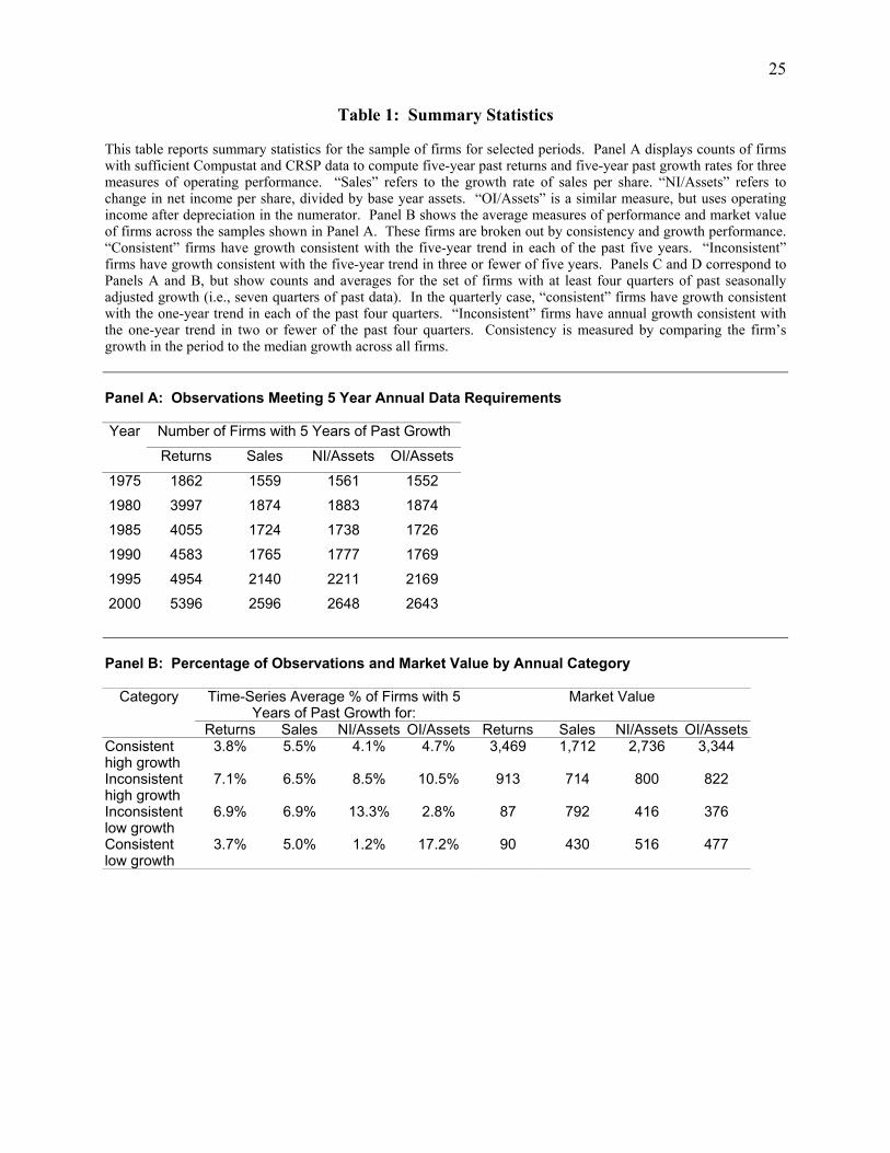
Table 1 reports summary statistics of the one- and five-year data sets. Counts of the five-

year sets of stocks in selected years are displayed in Table 1, Panel A. We report time series

averages of the proportion of firms with five years of past data that fall into consistent and

inconsistent groups on the right, as well as average market value in millions. The total number of

firms falling into high or low growth quintiles in a given year is 20%, by construction.

The sample contains roughly equal numbers of firms with five years of past reported

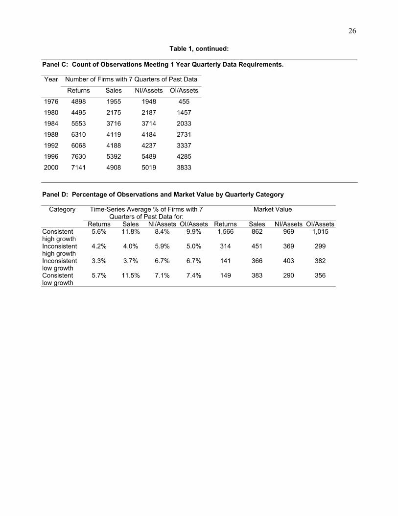
sales, net income over assets, and operating income over assets. Panels C and D of Table 1 show

the same summary statistics as Panels A and B, but for the set of firms with seven quarters of

past data for the calculation of four seasonal growth rates.

Overall, our data sets are relatively balanced between consistent and inconsistent groups.

For the five-year set, consistent high growers are much larger in size than inconsistent high

15

growers, yet they make up a smaller proportion of stocks. Consistent low growers are very

small, but not much smaller than inconsistent low growers. For the one-year set, the same

patterns hold, although consistent firms are relatively more common than inconsistent ones,

suggesting that performance is autocorrelated over shorter time frames. Size dispersion is less

among consistency groups for this set.

[Table 1]

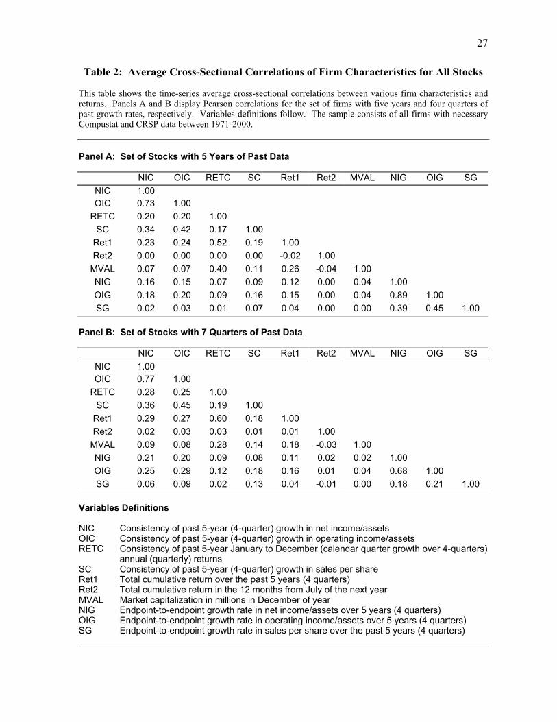
Cross-sectional correlations across our measures of the consistency of performance

appear in Table 2. Panel A reports the time series average of the cross-sectional correlation of

firm consistency ranks (across the four measures of growth), market values, five-year growth

rates, and future returns. The consistency statistics are positively correlated across measures, but

they are far from perfect substitutes. All are correlated with past returns and market values. The

OI measure is closely related to the net income measure. However, it is striking how little the

operating measures of consistency and growth co-move with the return based ones. This result

implies a difference between return-based predictability and accounting predictability. Panel B

tells a similar tale, although with one-year numbers.

[Table 2]

IV. Results

This section discusses the results of our medium- and long-horizon tests, consistency

tests, and tests examining returns following realizations that confirm or contradict a prior trend.

4.1 Medium Horizon Results

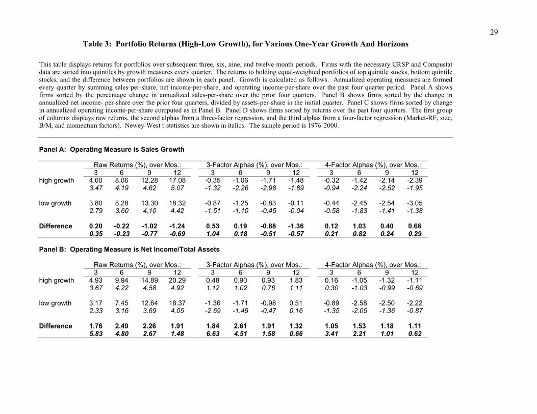
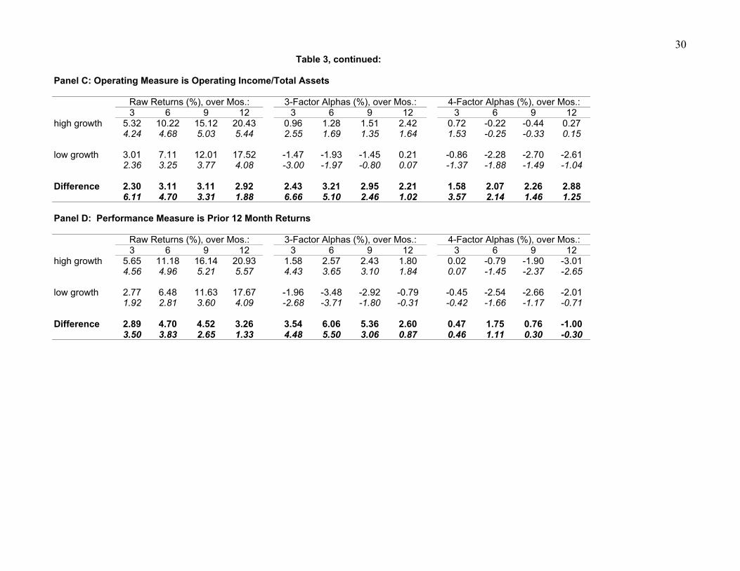
Table 3 reports the return performance of portfolios experiencing growing or declining

trends in a financial performance measure over the past four quarters. Returns are derived from a

strategy of buying an equal-weight portfolio of top-quintile growers and selling an equal-weight

portfolio of bottom-quintile growers. Raw returns over four horizons, three, six, nine, and 12

months, appear in the first four columns, followed by three-factor time series regression

intercepts (middle 4 columns), and four-factor regression intercepts (4 right columns). Return

performance is grouped in panels by growth metric.

16

We present returns to a price momentum strategy for comparison in panel D. These

results are consistent with previous research (Jagadeesh and Titman, 1993, and 2001). Firms

with high past 12-month returns (top quintile) exhibit significantly higher future returns over the

next three, six, nine-month horizons than firms with low past 12-month returns. This abnormal

performance is robust to three-factor controls. As expected, adding a fourth momentum factor,

UMD, eliminates the significance of momentum strategy profits.

We find that past “momentum” in financial performance also predicts future returns. For

the NI and OI measures, a strategy of buying past high growers and selling past low growers

earns 1.84% (t-stat 6.63) and 2.43% (t-stat 6.66), respectively, in the first 3 months using the

Fama-French three-factor model. A strategy based on sales growth, however, fails to generate

significant positive abnormal returns (3-factor alpha is 0.53%, t-statistic 1.04). The abnormal

performance for the NI and OI long-short strategies is similar as more months are added before

becoming indistinguishable from zero at 12 months. The last four columns show that the long-

short strategy’s performance is reduced when abnormal returns are estimated using the four-

factor model.

[Table 3]

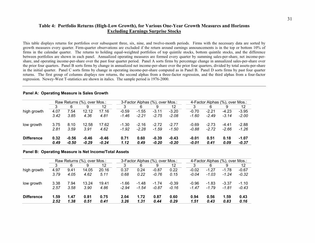
Discriminating between financial momentum and price momentum. The results in

Table 3 for financial momentum based long-short strategy could be due to post-earnings-

announcement drift (Ball and Brown, 1968, Foster, Ohlsen, and Shevlin, 1984, Bernard and

Thomas, 1989). We re-run the long-short strategies for the rolling four-quarter horizon, as in

Table 3, but eliminate all stocks selected by an earnings-surprise filter. This filter screens out

stocks that had returns in a three-day window around the earnings announcement in the top or

bottom quintiles of all such returns for all stocks within the latest quarter. Eliminating these

earnings surprise stocks is an extreme way of testing whether financial momentum is distinct

from drift. Both earnings surprise and financial momentum could theoretically be driven by the

same underreaction to operating results, and therefore would complement each other. However,

using the harsh filter allows us separate investors’ underreaction to short-term surprises (seen in

17

the earnings surprise filter) and to longer horizon trends (seen in the financial momentum

results).

When we eliminate these earnings surprise stocks, we find that abnormal returns to

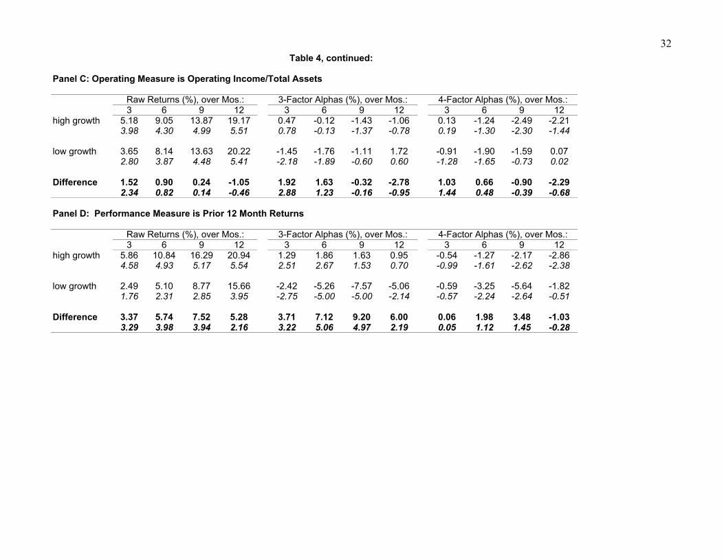
financial momentum are muted. Table 4 displays returns for this filtered set of stocks. The long-

short strategy based on NI and OI yields statistically significant abnormal return of

approximately two percent over a three-month period. However, over longer horizons of six-to-

12 months, neither NI nor OI-based momentum strategies generate significant abnormal returns.

As before, sales momentum is never profitable. The results offer weak evidence that investors

underreact to trends in performance beyond the surprise in earnings announcements.

[Table 4]

4.2 Long-Horizon Results

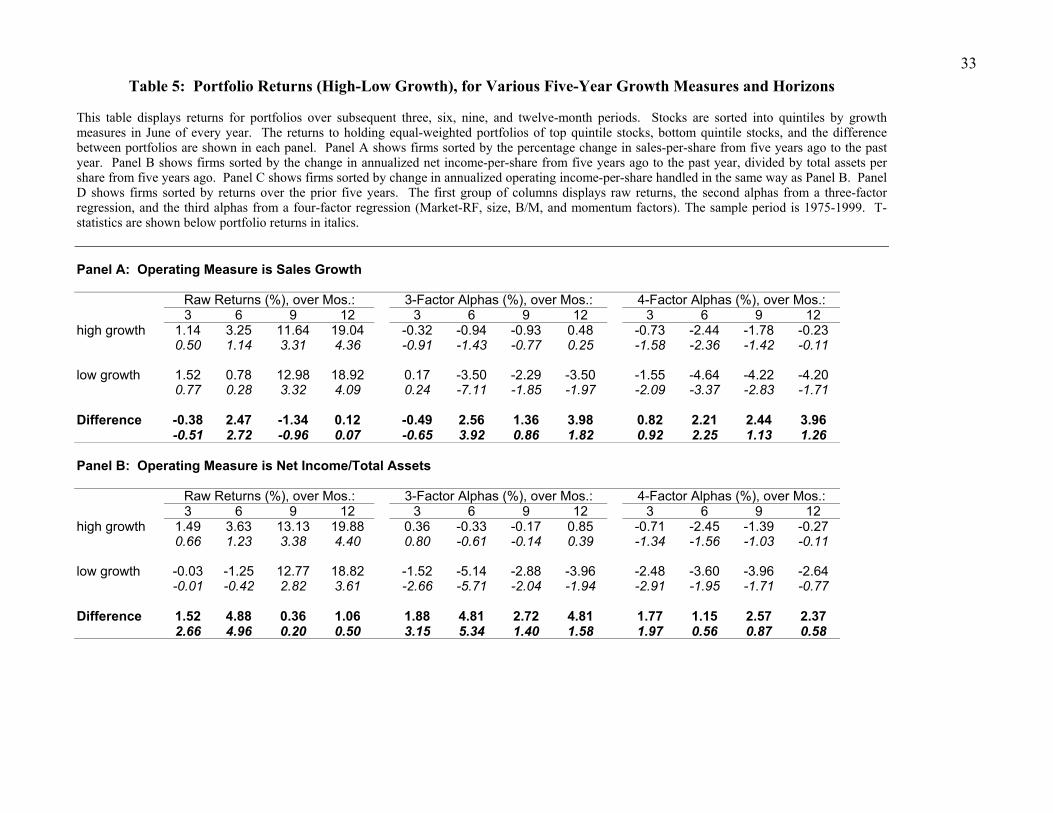
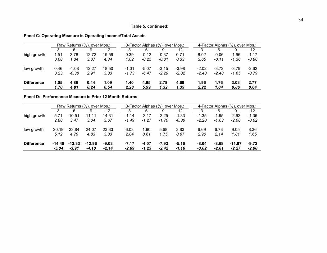
Table 5, Panels A-C report the raw and abnormal returns for portfolios formed on the

basis of five-year trends in sales, NI, and OI. We fail to find evidence of return reversals that

would be consistent with biased expectations attributable to the representativeness bias. The

point estimates of abnormal performance over three, six, nine and 12-month periods are almost

always positive, not negative. Recall that the strategy goes long in the best financial performance

quintile and short in the worst financial performance quintile. Therefore reversal implies

negative returns. The abnormal performance is occasionally significantly positive, but never

significantly negative.

Our evidence contradicts Lakonishok, Shleifer, and Vishny’s (LSV) (1994) findings for

the glamour vs. value stocks. Daniel and Titman (2001) provide a way to reconcile our results

with those of LSV. Daniel and Titman (2001) document a stronger negative relation between

expectations of future growth and future returns when growth cannot be explained by

fundamentals. They attribute their findings to investor overreaction to intangible information,

rather than tangible (i.e. fundamental or operating) information. Consistent with this view, while

we find no reversal following strong fundamental performance, results in panel D of Table 5

indicate reversals following extreme price performance over five years. (See DeBondt and

18

Thaler, 1985 and 1987, and Ball, Kothari, and Shanken, 1995, for past research on investor

overreaction).

[Table 5]

4.3 Results for Consistency of Financial Performance

Our next tests examine the effect of the pattern of prior performance on subsequent

returns. Specifically, we investigate whether consistent prior financial performance generates

less momentum and more reversal than inconsistent prior performance over medium and long

horizons. We detailed our methodology for sorting high and low growth firms by consistency in

section 3.1.

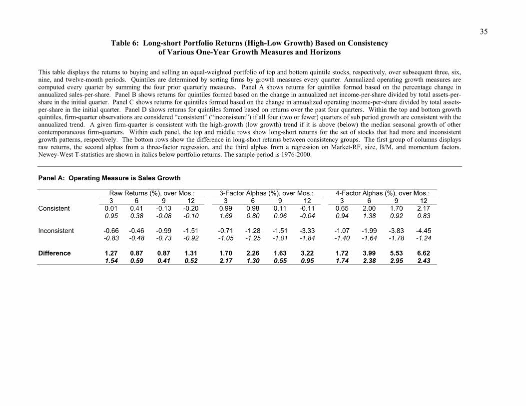
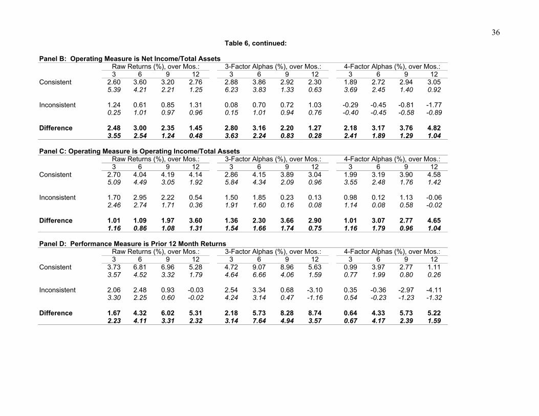
Table 6 shows the results when consistency of prior performance is measured on a

quarterly basis over the prior year. In this table, rows labeled “more consistent” (“less

consistent”) display returns to buying and selling the top and bottom quintiles of consistently

(inconsistently) performing firms. These rows therefore show how much return drift occurs for

consistent and inconsistent stocks. The rows labeled “difference” show the gap in returns

between the more and less consistent long-short strategies.

Returning to the predictions of some theories, all the entries in the “difference” row

should be negative. This is never the case. Table 6 shows that firms with inconsistent prior

performance have less return momentum than those with consistent performance, contrary to the

predictions of the behavioral theories based on representativeness bias. In line with Table 3, we

find no drift for firms sorted by sales-per-share growth. However, the drift that exists in the other

two financial growth measures, NI and OI, is greater in consistent stocks. To be sure, the

difference between consistent and inconsistent drift is rarely statistically significant across

horizons and measures. It is always positive, however, implying that investors underreact more

to trending performance that they have seen repeatedly than to flash-in-the-pan results.

[Table 6]

In Table 7, we repeat the tests in Table 6 using annual performance over the previous five

years to measure consistency. Again, according to the theories based on representativeness bias,

19

all entries in the “difference” rows should be negative because investors should form more biased

expectations about future performance for the stocks exhibiting a consistently growing financial

performance. As with the quarterly measurement period, this is not the case. For almost every

horizon, and every measure of growth, the post-portfolio formation returns of consistent firms are

statistically indistinguishable from those of inconsistent ones. In Table 5, we find no evidence

that investors extrapolate the growth trend and thus form biased expectations about future

growth. Table 7 affirms this view by showing that the past pattern of operating results also has

little effect on investor bias. In sum, tests using a number of performance measures, and two

conditioning horizons fail to uncover signs that the pattern of performance influences returns and

thus we are unable to show that representativeness or “law of small numbers”-based behavioral

biases systematically affect stock prices.

[Table 7]

As an additional test of whether or not the consistency of results affects security prices,

we focus on returns after a marginal period that confirms or disconfirms previously consistent (or

inconsistent) performance. The disconfirming signal in our test is an extra quarter (year) of

financial growth in the opposite direction as the trend for the past four quarters (five years).

Recall that we measure consistency over both past one year and past five years. We expect drift

in the direction of the disconfirming signal to be stronger following consistent prior results as

investors slowly change more strongly held priors.

Specifically, in the one-year period, steadier growth trends are more salient and thus

make underreaction less likely. Therefore, marginal signals that confirm the trend in investors’

minds should have little positive effect, while marginal signals that contradict the trend should

lead to reversal as investors slowly change their strongly held beliefs. For inconsistently growing

firms, the situation is reversed. Investors should hold weaker opinions about the existence of

growth trends and thus act more readily to the disconfirming signal. On the other hand, they will

be skeptical of a trend-confirming signal and thus underreact. Marginal trend-disconfirming

quarters do not tell investors anything new. In sum, inconsistent firms should display more drift

20

than consistent ones after confirming signals. They should also display less reversal after

disconfirming signals. Similar logic can be applied to the five-year context.

Taken together, this logic implies the following test. We form a long-short strategy of

buying high growth firms and selling low growth firms based on various performance measures.

This strategy should be less profitable for consistent firms than for inconsistent ones following a

confirming period, no matter the conditioning horizon. Moreover, it should be less profitable for

consistent firms than for inconsistent ones after a disconfirming period, no matter the horizon.

We provide the one-year horizon results in Table 8. The “difference” row shows the gap

in long-short profits between consistent and inconsistent sets. According to behavioral

arguments, this row should be negative in every case. Before discussing the difference row, we

note that, as expected, confirming financial performance always generates contemporaneous

positive returns and disconfirming performance generates negative returns. However, for the NI

and OI measures, both these returns trend for up to nine months after the marginal quarter. The

returns are also fairly robust to 3- and 4-factor adjustments. The results are more dramatic after

disconfirming quarters, which generate losses between –2% to –8% at 12 months, thus

reinforcing the existence of the “accounting momentum” documented in Table 3. However, for

the sales-per-share measure, only disconfirming information causes persistent and economically

sizeable reversal (-5% to –6%), which is also in line with our previous results.

[Table 8]

We next examine whether consistency of prior performance affects the magnitude of this

momentum and reversal in the face of marginal information. In general, the results do not show

any difference in returns. Hardly any of the entries in the difference row are statistically

significant at the 5% level, and point estimates are often positive. Three- and four-factor

adjustments do no change this conclusion. Again, we confirm the results of Table 6. We find no

evidence that the past pattern of returns causes investors to form biased expectations about future

performance

21

We run similar tests on the five-year sets of stocks. In these tests, we consider the effects

of a marginal year of operating performance on concurrent and subsequent year returns. The

results are shown in Table 9. We find no evidence that focusing on consistent performers

increases the reversal effect following a disconfirming year. The statistical weakness of the

results can be attributed to having fewer observations, as well as the long return-measurement

window. However, the point estimates are often positive, contrary to what we would expect if

consistency affected expectations.8

[Table 9]

V. Conclusions

Many stories about investor behavior rely on some form of the representativeness heuristic.

This heuristic can lead them to form biased expectations. In a typical behavioral financial model,

investors mentally misplace firms into various groups based on the past performance, and are

subsequently surprised or disappointed in predictable ways. This surprise is reflected in returns.

We use accounting data to test whether investors’ tendency classify firms into groups

influences security return behavior as modeled in the behavioral finance theories. We use trends

and sequences of accounting performance to separate firms into high and low growth and further

divide them by consistency of growth patterns. The advantage of this approach is that we use a

specific source of information to model possible investor categories in a simple and

straightforward way. Furthermore, our approach provides out-of-sample tests of the idea that

investors under or over-react to past information. Finally, we use different horizons and growth

metrics to allow for the different information investors could use.

Consistent with findings in previous research, we find evidence of multi-month momentum

in returns after accounting performance. However, this momentum is substantially reduced when

8 The numbers in the difference row are often not the exact arithmetic difference between consistent and inconsistent groups, because in some periods we have no inconsistently growing firms that also have disconfirming marginal years. Therefore we do not have the difference in some years.

22

we control for earnings surprise effects. We find no support for multi-year reversal related to

past accounting performance. Finally, we find little evidence that conditioning on the

consistency of past growth rates improves return predictability. Our evidence indicates that the

sequence of past accounting performance is not related to future returns, and therefore is unlikely

to bias investors’ consensus expectations.

Overall, these results suggest that multi-month momentum and long-term reversal are not

due investors’ mental biases as modeled in the behavioral theories and/or the maintained

hypothesis of limited arbitrage is not descriptive. Our results suggest pricing is not as if investors

extrapolate firms’ growth rates too far into the future. Nor do investors seem to underreact to

incipient trends in performance. All of these conclusions cast doubt on the representativeness

heuristic-based theories of behavioral finance.

One could conclude that representativeness has no place in describing stock return behavior

(and also perhaps investor behavior). However, the predictability of returns documented in the

literature remains an interesting and problematic phenomenon potentially at odds with market

efficiency. Investors may think in categories, but using current theory as our guide, we are

unable to the stock price implications predicted in those theories. Alternatively, we failed to

identify the correct categories, metrics, or horizons necessary to document the consequences of

behavioral information processing biases. Our evidence poses a challenge to behavioral finance

theories and therefore researchers should consider refining their models to guide further

empirical work.

23

VI. References

Ball, R., Brown, P., 1968, “An empirical evaluation of accounting income numbers,” Journal of Accounting Research 6, 159-178.

Ball, R., Kothari, S., Shanken, J., 1995, Problems in measuring portfolio performance: An application to contrarian investment strategies, Journal of Financial Economics 38, 79-107.

Barberis, N., Shleifer, A., Vishny, R., 1998, A model of investor sentiment, Journal of Financial Economics 49, 307-343.

Barth, M., Elliot, J., Finn, M., 1999, Market rewards associated with patterns of increasing earnings, Journal of Accounting Research 37, 387-413.

Bernard, V., Thomas, J., 1989, Post-earnings-announcement drift: Delayed price response or risk premium?, Journal of Accounting Research 27, 1-36.

Bernard, V., Thomas, J., 1990, Evidence that stock prices do not fully reflect the implications of current earnings for future earnings, Journal of Accounting and Economics 13, 305-340.

Carhart, M., 1997, On persistence in mutual fund performance, Journal of Finance 52, 57-82.

Cohen, R., Gompers, P., Vuolteenaho, T., 2001, Who underreacts to cash-flow news? Evidence from trading between individuals and institutions, Harvard University, working Paper.

Daniel, K., Hirshleifer, D., Subrahmanyam, A., 1998, Investor psychology and security market under- and overreactions, Journal of Finance 53, 1839-1885.

Daniel, K., Hirshleifer, D., Teoh, S., 2002, Investor psychology in capital markets: evidence and policy implications, Journal of Monetary Economics 49, 139-209.

Daniel, K., Titman, S., 2001, Market reactions to tangible and intangible information, Northwestern University Working paper.

De Long, J., Shleifer, A., Vishny, R., Waldman, R., 1990, Noise trader risk in financial markets, Journal of Political Economy 98, 703-738.

DeBondt, W., Thaler, R., 1985, Does the stock market overreact? Journal of Finance 40, 793-805.

DeBondt, W., Thaler, R., 1987, Further evidence of investor overreaction and stock market seasonality, Journal of Finance 42, 557-581.

Dechow, P., Sloan, R., 1997, Returns to contrarian investment strategies: Tests of naïve expectations hypotheses, Journal of Financial Economics 43, 3-27.

Fama, E., 1991, Efficient Capital Markets: II, Journal of Finance 46, 1575-1617.

Fama, E., 1998, Market efficiency, long run returns, and behavioral finance, Journal of Financial Economics 49, 283-306.

24

Foster, G., Olsen, C., Shevlin, T., 1984, Earnings releases, anomalies, and the behavior of security returns, Accounting Review 59, 574-603.

Givoly, D., Palmon, D., 1982, Timeliness of annual earnings announcements: Some empirical evidence, Accounting Review 57, 486-508.

Hirshleifer, D., 2001 Investor psychology and asset pricing, Journal of Finance 56, 1533-1598.

Hong, H., Stein, J., 1999, A unified theory of underrreaction, momentum trading, and overreaction in asset markets, Journal of Finance 54, 2143-2184.

Jagadeesh, N., Titman, S., 1993, Returns to buying winners and selling losers: Implications for stock market efficiency, Journal of Finance 48, 65-91.

Jagadeesh, N., Titman, S., 2001, Profitability of momentum strategies: An evaluation of alternative explanations, Journal of Finance 56, 699-720.

La Porta, R., Lakonishok, J., Shleifer, A., Vishny, R., 1997, Good news for value stocks: Further evidence on market efficiency, Journal of Finance, 859-874.

Lakonishok, J., Shleifer, A., Vishny, R., 1994, Contrarian investment, extrapolation, and risk, Journal of Finance 49, 1541-1578.

Miller, M., 1986, Behavioral rationality in finance: The case of dividends, Journal of Business 59, S451-S486.

Mullainathan, S., 2001, Thinking through categories, NBER Working Paper.

Rabin, M., 2001, Inference by Believers in the Law of Small Numbers, Quarterly Journal of Economics, forthcoming.

Rubinstein, M., 2001, Rational markets: yes or no? The affirmative case, Financial Analysts Journal, forthcoming.

Shiller, R., 1999, Human behavior and the efficiency of the financial system, in Handbook of Macroeconomics 1, 1305-1340.

Shleifer, A., 2000, Inefficient markets: An introduction to behavioral finance, Oxford University Press, Oxford, United Kingdom.

Shliefer, A., Vishny, R., 1997, The limits of arbitrage, Journal of Finance 52, 35-55.

Sirri E., Tufano P., 1998, Costly search and mutual fund flows, Journal of Finance 53, 1589-1622.

Tversky, A., Kahneman, D., 1974, Judgement under uncertainty: Heuristics and biases, Science 185, 1124-1131.

25

Table 1: Summary Statistics This table reports summary statistics for the sample of firms for selected periods. Panel A displays counts of firms with sufficient Compustat and CRSP data to compute five-year past returns and five-year past growth rates for three measures of operating performance. “Sales” refers to the growth rate of sales per share. “NI/Assets” refers to change in net income per share, divided by base year assets. “OI/Assets” is a similar measure, but uses operating income after depreciation in the numerator. Panel B shows the average measures of performance and market value of firms across the samples shown in Panel A. These firms are broken out by consistency and growth performance. “Consistent” firms have growth consistent with the five-year trend in each of the past five years. “Inconsistent” firms have growth consistent with the five-year trend in three or fewer of five years. Panels C and D correspond to Panels A and B, but show counts and averages for the set of firms with at least four quarters of past seasonally adjusted growth (i.e., seven quarters of past data). In the quarterly case, “consistent” firms have growth consistent with the one-year trend in each of the past four quarters. “Inconsistent” firms have annual growth consistent with the one-year trend in two or fewer of the past four quarters. Consistency is measured by comparing the firm’s growth in the period to the median growth across all firms. Panel A: Observations Meeting 5 Year Annual Data Requirements Year Number of Firms with 5 Years of Past Growth

Returns Sales NI/Assets OI/Assets

1975 1862 1559 1561 1552 1980 3997 1874 1883 1874 1985 4055 1724 1738 1726 1990 4583 1765 1777 1769 1995 4954 2140 2211 2169 2000 5396 2596 2648 2643 Panel B: Percentage of Observations and Market Value by Annual Category

Category Time-Series Average % of Firms with 5 Years of Past Growth for:

Market Value

Returns Sales NI/Assets OI/Assets Returns Sales NI/Assets OI/AssetsConsistent high growth

3.8% 5.5% 4.1% 4.7% 3,469 1,712 2,736 3,344

Inconsistent high growth

7.1% 6.5% 8.5% 10.5% 913 714 800 822

Inconsistent low growth

6.9% 6.9% 13.3% 2.8% 87 792 416 376

Consistent low growth

3.7% 5.0% 1.2% 17.2% 90 430 516 477

26

Table 1, continued:

Panel C: Count of Observations Meeting 1 Year Quarterly Data Requirements. Year Number of Firms with 7 Quarters of Past Data

Returns Sales NI/Assets OI/Assets

1976 4898 1955 1948 455 1980 4495 2175 2187 1457 1984 5553 3716 3714 2033 1988 6310 4119 4184 2731 1992 6068 4188 4237 3337 1996 7630 5392 5489 4285 2000 7141 4908 5019 3833

Panel D: Percentage of Observations and Market Value by Quarterly Category

Category Time-Series Average % of Firms with 7 Quarters of Past Data for:

Market Value

Returns Sales NI/Assets OI/Assets Returns Sales NI/Assets OI/AssetsConsistent high growth

5.6% 11.8% 8.4% 9.9% 1,566 862 969 1,015

Inconsistent high growth

4.2% 4.0% 5.9% 5.0% 314 451 369 299

Inconsistent low growth

3.3% 3.7% 6.7% 6.7% 141 366 403 382

Consistent low growth

5.7% 11.5% 7.1% 7.4% 149 383 290 356

27

Table 2: Average Cross-Sectional Correlations of Firm Characteristics for All Stocks This table shows the time-series average cross-sectional correlations between various firm characteristics and returns. Panels A and B display Pearson correlations for the set of firms with five years and four quarters of past growth rates, respectively. Variables definitions follow. The sample consists of all firms with necessary Compustat and CRSP data between 1971-2000. Panel A: Set of Stocks with 5 Years of Past Data

NIC OIC RETC SC Ret1 Ret2 MVAL NIG OIG SG NIC 1.00 OIC 0.73 1.00

RETC 0.20 0.20 1.00 SC 0.34 0.42 0.17 1.00

Ret1 0.23 0.24 0.52 0.19 1.00 Ret2 0.00 0.00 0.00 0.00 -0.02 1.00

MVAL 0.07 0.07 0.40 0.11 0.26 -0.04 1.00 NIG 0.16 0.15 0.07 0.09 0.12 0.00 0.04 1.00 OIG 0.18 0.20 0.09 0.16 0.15 0.00 0.04 0.89 1.00 SG 0.02 0.03 0.01 0.07 0.04 0.00 0.00 0.39 0.45 1.00

Panel B: Set of Stocks with 7 Quarters of Past Data

NIC OIC RETC SC Ret1 Ret2 MVAL NIG OIG SG NIC 1.00 OIC 0.77 1.00

RETC 0.28 0.25 1.00 SC 0.36 0.45 0.19 1.00

Ret1 0.29 0.27 0.60 0.18 1.00 Ret2 0.02 0.03 0.03 0.01 0.01 1.00

MVAL 0.09 0.08 0.28 0.14 0.18 -0.03 1.00 NIG 0.21 0.20 0.09 0.08 0.11 0.02 0.02 1.00 OIG 0.25 0.29 0.12 0.18 0.16 0.01 0.04 0.68 1.00 SG 0.06 0.09 0.02 0.13 0.04 -0.01 0.00 0.18 0.21 1.00

Variables Definitions NIC Consistency of past 5-year (4-quarter) growth in net income/assets OIC Consistency of past 5-year (4-quarter) growth in operating income/assets RETC Consistency of past 5-year January to December (calendar quarter growth over 4-quarters)

annual (quarterly) returns SC Consistency of past 5-year (4-quarter) growth in sales per share Ret1 Total cumulative return over the past 5 years (4 quarters) Ret2 Total cumulative return in the 12 months from July of the next year MVAL Market capitalization in millions in December of year NIG Endpoint-to-endpoint growth rate in net income/assets over 5 years (4 quarters) OIG Endpoint-to-endpoint growth rate in operating income/assets over 5 years (4 quarters) SG Endpoint-to-endpoint growth rate in sales per share over the past 5 years (4 quarters)

29

Table 3: Portfolio Returns (High-Low Growth), for Various One-Year Growth And Horizons This table displays returns for portfolios over subsequent three, six, nine, and twelve-month periods. Firms with the necessary CRSP and Compustat data are sorted into quintiles by growth measures every quarter. The returns to holding equal-weighted portfolios of top quintile stocks, bottom quintile stocks, and the difference between portfolios are shown in each panel. Growth is calculated as follows. Annualized operating measures are formed every quarter by summing sales-per-share, net income-per-share, and operating income-per-share over the past four quarter period. Panel A shows firms sorted by the percentage change in annualized sales-per-share over the prior four quarters. Panel B shows firms sorted by the change in annualized net income- per-share over the prior four quarters, divided by assets-per-share in the initial quarter. Panel C shows firms sorted by change in annualized operating income-per-share computed as in Panel B. Panel D shows firms sorted by returns over the past four quarters. The first group of columns displays raw returns, the second alphas from a three-factor regression, and the third alphas from a four-factor regression (Market-RF, size, B/M, and momentum factors). Newey-West t-statistics are shown in italics. The sample period is 1976-2000. Panel A: Operating Measure is Sales Growth Raw Returns (%), over Mos.: 3-Factor Alphas (%), over Mos.: 4-Factor Alphas (%), over Mos.: 3 6 9 12 3 6 9 12 3 6 9 12 high growth 4.00 8.06 12.28 17.08 -0.35 -1.06 -1.71 -1.48 -0.32 -1.42 -2.14 -2.39 3.47 4.19 4.62 5.07 -1.32 -2.26 -2.98 -1.89 -0.94 -2.24 -2.52 -1.95 low growth 3.80 8.28 13.30 18.32 -0.87 -1.25 -0.83 -0.11 -0.44 -2.45 -2.54 -3.05 2.79 3.60 4.10 4.42 -1.51 -1.10 -0.45 -0.04 -0.58 -1.83 -1.41 -1.38 Difference 0.20 -0.22 -1.02 -1.24 0.53 0.19 -0.88 -1.36 0.12 1.03 0.40 0.66 0.35 -0.23 -0.77 -0.69 1.04 0.18 -0.51 -0.57 0.21 0.82 0.24 0.29 Panel B: Operating Measure is Net Income/Total Assets Raw Returns (%), over Mos.: 3-Factor Alphas (%), over Mos.: 4-Factor Alphas (%), over Mos.: 3 6 9 12 3 6 9 12 3 6 9 12 high growth 4.93 9.94 14.89 20.29 0.48 0.90 0.93 1.83 0.16 -1.05 -1.32 -1.11 3.67 4.22 4.58 4.92 1.12 1.02 0.76 1.11 0.30 -1.03 -0.99 -0.69 low growth 3.17 7.45 12.64 18.37 -1.36 -1.71 -0.98 0.51 -0.89 -2.58 -2.50 -2.22 2.33 3.16 3.69 4.05 -2.69 -1.49 -0.47 0.16 -1.35 -2.05 -1.36 -0.87 Difference 1.76 2.49 2.26 1.91 1.84 2.61 1.91 1.32 1.05 1.53 1.18 1.11 5.83 4.80 2.67 1.48 6.63 4.51 1.58 0.66 3.41 2.21 1.01 0.62

30

Table 3, continued:

Panel C: Operating Measure is Operating Income/Total Assets Raw Returns (%), over Mos.: 3-Factor Alphas (%), over Mos.: 4-Factor Alphas (%), over Mos.: 3 6 9 12 3 6 9 12 3 6 9 12 high growth 5.32 10.22 15.12 20.43 0.96 1.28 1.51 2.42 0.72 -0.22 -0.44 0.27 4.24 4.68 5.03 5.44 2.55 1.69 1.35 1.64 1.53 -0.25 -0.33 0.15 low growth 3.01 7.11 12.01 17.52 -1.47 -1.93 -1.45 0.21 -0.86 -2.28 -2.70 -2.61 2.36 3.25 3.77 4.08 -3.00 -1.97 -0.80 0.07 -1.37 -1.88 -1.49 -1.04 Difference 2.30 3.11 3.11 2.92 2.43 3.21 2.95 2.21 1.58 2.07 2.26 2.88 6.11 4.70 3.31 1.88 6.66 5.10 2.46 1.02 3.57 2.14 1.46 1.25 Panel D: Performance Measure is Prior 12 Month Returns Raw Returns (%), over Mos.: 3-Factor Alphas (%), over Mos.: 4-Factor Alphas (%), over Mos.: 3 6 9 12 3 6 9 12 3 6 9 12 high growth 5.65 11.18 16.14 20.93 1.58 2.57 2.43 1.80 0.02 -0.79 -1.90 -3.01 4.56 4.96 5.21 5.57 4.43 3.65 3.10 1.84 0.07 -1.45 -2.37 -2.65 low growth 2.77 6.48 11.63 17.67 -1.96 -3.48 -2.92 -0.79 -0.45 -2.54 -2.66 -2.01 1.92 2.81 3.60 4.09 -2.68 -3.71 -1.80 -0.31 -0.42 -1.66 -1.17 -0.71 Difference 2.89 4.70 4.52 3.26 3.54 6.06 5.36 2.60 0.47 1.75 0.76 -1.00 3.50 3.83 2.65 1.33 4.48 5.50 3.06 0.87 0.46 1.11 0.30 -0.30

31

Table 4: Portfolio Returns (High-Low Growth), for Various One-Year Growth Measures and Horizons Excluding Earnings Surprise Stocks

This table displays returns for portfolios over subsequent three, six, nine, and twelve-month periods. Firms with the necessary data are sorted by growth measures every quarter. Firm-quarter observations are excluded if the return around earnings announcements is in the top or bottom 10% of firms in the calendar quarter. The returns to holding equal-weighted portfolios of top quintile stocks, bottom quintile stocks, and the difference between portfolios are shown in each panel. Annualized operating measures are formed every quarter by summing sales-per-share, net income-per-share, and operating income-per-share over the past four quarter period. Panel A sorts firms by percentage change in annualized sales-per-share over the prior four quarters. Panel B sorts firms by change in annualized net income-per-share over the prior four quarters, divided by total assets-per-share in the initial quarter. Panel C sorts firms by change in operating income-per-share computed as in Panel B. Panel D sorts firms by past four quarter returns. The first group of columns displays raw returns, the second alphas from a three-factor regression, and the third alphas from a four-factor regression. Newey-West T-statistics are shown in italics. The sample period is 1976-2000. Panel A: Operating Measure is Sales Growth Raw Returns (%), over Mos.: 3-Factor Alphas (%), over Mos.: 4-Factor Alphas (%), over Mos.: 3 6 9 12 3 6 9 12 3 6 9 12 high growth 4.07 7.54 12.12 17.16 -0.59 -1.55 -3.11 -3.20 -0.70 -2.21 -4.23 -3.95 3.42 3.85 4.36 4.81 -1.46 -2.21 -2.75 -2.08 -1.60 -2.49 -3.14 -2.00 low growth 3.75 8.10 12.58 17.62 -1.30 -2.16 -2.72 -2.77 -0.69 -2.73 -4.41 -2.88 2.81 3.59 3.91 4.62 -1.92 -2.28 -1.59 -1.50 -0.88 -2.72 -2.66 -1.26 Difference 0.32 -0.56 -0.46 -0.46 0.71 0.60 -0.39 -0.43 -0.01 0.51 0.18 -1.07 0.49 -0.50 -0.29 -0.24 1.12 0.49 -0.20 -0.20 -0.01 0.41 0.09 -0.37

Panel B: Operating Measure is Net Income/Total Assets Raw Returns (%), over Mos.: 3-Factor Alphas (%), over Mos.: 4-Factor Alphas (%), over Mos.: 3 6 9 12 3 6 9 12 3 6 9 12 high growth 4.97 9.41 14.05 20.16 0.37 0.24 -0.87 0.22 -0.02 -1.27 -1.78 -0.67 3.79 4.05 4.62 5.11 0.68 0.22 -0.76 0.15 -0.04 -1.03 -1.24 -0.32 low growth 3.38 7.94 13.24 19.41 -1.66 -1.48 -1.74 -0.39 -0.96 -1.83 -3.37 -1.10 2.57 3.58 3.90 4.86 -2.94 -1.54 -0.87 -0.16 -1.47 -1.79 -1.81 -0.43 Difference 1.59 1.47 0.81 0.75 2.04 1.72 0.87 0.60 0.94 0.56 1.59 0.43 2.52 1.38 0.51 0.41 3.26 1.31 0.44 0.29 1.51 0.43 0.83 0.16

32

Table 4, continued: Panel C: Operating Measure is Operating Income/Total Assets Raw Returns (%), over Mos.: 3-Factor Alphas (%), over Mos.: 4-Factor Alphas (%), over Mos.: 3 6 9 12 3 6 9 12 3 6 9 12 high growth 5.18 9.05 13.87 19.17 0.47 -0.12 -1.43 -1.06 0.13 -1.24 -2.49 -2.21 3.98 4.30 4.99 5.51 0.78 -0.13 -1.37 -0.78 0.19 -1.30 -2.30 -1.44 low growth 3.65 8.14 13.63 20.22 -1.45 -1.76 -1.11 1.72 -0.91 -1.90 -1.59 0.07 2.80 3.87 4.48 5.41 -2.18 -1.89 -0.60 0.60 -1.28 -1.65 -0.73 0.02 Difference 1.52 0.90 0.24 -1.05 1.92 1.63 -0.32 -2.78 1.03 0.66 -0.90 -2.29 2.34 0.82 0.14 -0.46 2.88 1.23 -0.16 -0.95 1.44 0.48 -0.39 -0.68 Panel D: Performance Measure is Prior 12 Month Returns Raw Returns (%), over Mos.: 3-Factor Alphas (%), over Mos.: 4-Factor Alphas (%), over Mos.: 3 6 9 12 3 6 9 12 3 6 9 12 high growth 5.86 10.84 16.29 20.94 1.29 1.86 1.63 0.95 -0.54 -1.27 -2.17 -2.86 4.58 4.93 5.17 5.54 2.51 2.67 1.53 0.70 -0.99 -1.61 -2.62 -2.38 low growth 2.49 5.10 8.77 15.66 -2.42 -5.26 -7.57 -5.06 -0.59 -3.25 -5.64 -1.82 1.76 2.31 2.85 3.95 -2.75 -5.00 -5.00 -2.14 -0.57 -2.24 -2.64 -0.51 Difference 3.37 5.74 7.52 5.28 3.71 7.12 9.20 6.00 0.06 1.98 3.48 -1.03 3.29 3.98 3.94 2.16 3.22 5.06 4.97 2.19 0.05 1.12 1.45 -0.28

33

Table 5: Portfolio Returns (High-Low Growth), for Various Five-Year Growth Measures and Horizons

This table displays returns for portfolios over subsequent three, six, nine, and twelve-month periods. Stocks are sorted into quintiles by growth measures in June of every year. The returns to holding equal-weighted portfolios of top quintile stocks, bottom quintile stocks, and the difference between portfolios are shown in each panel. Panel A shows firms sorted by the percentage change in sales-per-share from five years ago to the past year. Panel B shows firms sorted by the change in annualized net income-per-share from five years ago to the past year, divided by total assets per share from five years ago. Panel C shows firms sorted by change in annualized operating income-per-share handled in the same way as Panel B. Panel D shows firms sorted by returns over the prior five years. The first group of columns displays raw returns, the second alphas from a three-factor regression, and the third alphas from a four-factor regression (Market-RF, size, B/M, and momentum factors). The sample period is 1975-1999. T-statistics are shown below portfolio returns in italics. Panel A: Operating Measure is Sales Growth Raw Returns (%), over Mos.: 3-Factor Alphas (%), over Mos.: 4-Factor Alphas (%), over Mos.: 3 6 9 12 3 6 9 12 3 6 9 12 high growth 1.14 3.25 11.64 19.04 -0.32 -0.94 -0.93 0.48 -0.73 -2.44 -1.78 -0.23 0.50 1.14 3.31 4.36 -0.91 -1.43 -0.77 0.25 -1.58 -2.36 -1.42 -0.11 low growth 1.52 0.78 12.98 18.92 0.17 -3.50 -2.29 -3.50 -1.55 -4.64 -4.22 -4.20 0.77 0.28 3.32 4.09 0.24 -7.11 -1.85 -1.97 -2.09 -3.37 -2.83 -1.71 Difference -0.38 2.47 -1.34 0.12 -0.49 2.56 1.36 3.98 0.82 2.21 2.44 3.96 -0.51 2.72 -0.96 0.07 -0.65 3.92 0.86 1.82 0.92 2.25 1.13 1.26

Panel B: Operating Measure is Net Income/Total Assets Raw Returns (%), over Mos.: 3-Factor Alphas (%), over Mos.: 4-Factor Alphas (%), over Mos.: 3 6 9 12 3 6 9 12 3 6 9 12 high growth 1.49 3.63 13.13 19.88 0.36 -0.33 -0.17 0.85 -0.71 -2.45 -1.39 -0.27 0.66 1.23 3.38 4.40 0.80 -0.61 -0.14 0.39 -1.34 -1.56 -1.03 -0.11 low growth -0.03 -1.25 12.77 18.82 -1.52 -5.14 -2.88 -3.96 -2.48 -3.60 -3.96 -2.64 -0.01 -0.42 2.82 3.61 -2.66 -5.71 -2.04 -1.94 -2.91 -1.95 -1.71 -0.77 Difference 1.52 4.88 0.36 1.06 1.88 4.81 2.72 4.81 1.77 1.15 2.57 2.37 2.66 4.96 0.20 0.50 3.15 5.34 1.40 1.58 1.97 0.56 0.87 0.58

34

Table 5, continued:

Panel C: Operating Measure is Operating Income/Total Assets Raw Returns (%), over Mos.: 3-Factor Alphas (%), over Mos.: 4-Factor Alphas (%), over Mos.: 3 6 9 12 3 6 9 12 3 6 9 12 high growth 1.51 3.78 12.72 19.59 0.39 -0.12 -0.37 0.71 8.02 -0.06 -1.96 -1.17 0.68 1.34 3.37 4.34 1.02 -0.25 -0.31 0.33 3.65 -0.11 -1.36 -0.86 low growth 0.46 -1.08 12.27 18.50 -1.01 -5.07 -3.15 -3.98 -2.02 -3.72 -3.79 -2.62 0.23 -0.38 2.91 3.83 -1.73 -6.47 -2.29 -2.02 -2.48 -2.48 -1.65 -0.79 Difference 1.05 4.86 0.44 1.09 1.40 4.95 2.78 4.69 1.96 1.76 3.03 2.77 1.70 4.81 0.24 0.54 2.28 5.99 1.32 1.39 2.22 1.04 0.86 0.64 Panel D: Performance Measure is Prior 12 Month Returns Raw Returns (%), over Mos.: 3-Factor Alphas (%), over Mos.: 4-Factor Alphas (%), over Mos.: 3 6 9 12 3 6 9 12 3 6 9 12 high growth 5.71 10.51 11.11 14.31 -1.14 -2.17 -2.25 -1.33 -1.35 -1.95 -2.92 -1.36 2.88 3.47 3.04 3.67 -1.49 -1.27 -1.70 -0.80 -2.20 -1.63 -2.08 -0.62 low growth 20.19 23.84 24.07 23.33 6.03 1.90 5.68 3.83 6.69 6.73 9.05 8.36 5.12 4.79 4.83 3.83 2.84 0.61 1.75 0.87 2.90 2.14 1.81 1.65 Difference -14.48 -13.33 -12.96 -9.03 -7.17 -4.07 -7.93 -5.16 -8.04 -8.68 -11.97 -9.72 -5.04 -3.91 -4.10 -2.14 -2.69 -1.23 -2.42 -1.16 -3.02 -2.61 -2.27 -2.00

35

Table 6: Long-short Portfolio Returns (High-Low Growth) Based on Consistency of Various One-Year Growth Measures and Horizons

This table displays the returns to buying and selling an equal-weighted portfolio of top and bottom quintile stocks, respectively, over subsequent three, six, nine, and twelve-month periods. Quintiles are determined by sorting firms by growth measures every quarter. Annualized operating growth measures are computed every quarter by summing the four prior quarterly measures. Panel A shows returns for quintiles formed based on the percentage change in annualized sales-per-share. Panel B shows returns for quintiles formed based on the change in annualized net income-per-share divided by total assets-per-share in the initial quarter. Panel C shows returns for quintiles formed based on the change in annualized operating income-per-share divided by total assets-per-share in the initial quarter. Panel D shows returns for quintiles formed based on returns over the past four quarters. Within the top and bottom growth quintiles, firm-quarter observations are considered “consistent” (“inconsistent”) if all four (two or fewer) quarters of sub period growth are consistent with the annualized trend. A given firm-quarter is consistent with the high-growth (low growth) trend if it is above (below) the median seasonal growth of other contemporaneous firm-quarters. Within each panel, the top and middle rows show long-short returns for the set of stocks that had more and inconsistent growth patterns, respectively. The bottom rows show the difference in long-short returns between consistency groups. The first group of columns displays raw returns, the second alphas from a three-factor regression, and the third alphas from a regression on Market-RF, size, B/M, and momentum factors. Newey-West T-statistics are shown in italics below portfolio returns. The sample period is 1976-2000. Panel A: Operating Measure is Sales Growth Raw Returns (%), over Mos.: 3-Factor Alphas (%), over Mos.: 4-Factor Alphas (%), over Mos.: 3 6 9 12 3 6 9 12 3 6 9 12 Consistent 0.01 0.41 -0.13 -0.20 0.99 0.98 0.11 -0.11 0.65 2.00 1.70 2.17 0.95 0.38 -0.08 -0.10 1.69 0.80 0.06 -0.04 0.94 1.38 0.92 0.83 Inconsistent -0.66 -0.46 -0.99 -1.51 -0.71 -1.28 -1.51 -3.33 -1.07 -1.99 -3.83 -4.45 -0.83 -0.48 -0.73 -0.92 -1.05 -1.25 -1.01 -1.84 -1.40 -1.64 -1.78 -1.24 Difference 1.27 0.87 0.87 1.31 1.70 2.26 1.63 3.22 1.72 3.99 5.53 6.62 1.54 0.59 0.41 0.52 2.17 1.30 0.55 0.95 1.74 2.38 2.95 2.43

36

Table 6, continued:

Panel B: Operating Measure is Net Income/Total Assets Raw Returns (%), over Mos.: 3-Factor Alphas (%), over Mos.: 4-Factor Alphas (%), over Mos.: 3 6 9 12 3 6 9 12 3 6 9 12 Consistent 2.60 3.60 3.20 2.76 2.88 3.86 2.92 2.30 1.89 2.72 2.94 3.05 5.39 4.21 2.21 1.25 6.23 3.83 1.33 0.63 3.69 2.45 1.40 0.92 Inconsistent 1.24 0.61 0.85 1.31 0.08 0.70 0.72 1.03 -0.29 -0.45 -0.81 -1.77 0.25 1.01 0.97 0.96 0.15 1.01 0.94 0.76 -0.40 -0.45 -0.58 -0.89 Difference 2.48 3.00 2.35 1.45 2.80 3.16 2.20 1.27 2.18 3.17 3.76 4.82 3.55 2.54 1.24 0.48 3.63 2.24 0.83 0.28 2.41 1.89 1.29 1.04 Panel C: Operating Measure is Operating Income/Total Assets Raw Returns (%), over Mos.: 3-Factor Alphas (%), over Mos.: 4-Factor Alphas (%), over Mos.: 3 6 9 12 3 6 9 12 3 6 9 12 Consistent 2.70 4.04 4.19 4.14 2.86 4.15 3.89 3.04 1.99 3.19 3.90 4.58 5.09 4.49 3.05 1.92 5.84 4.34 2.09 0.96 3.55 2.48 1.76 1.42 Inconsistent 1.70 2.95 2.22 0.54 1.50 1.85 0.23 0.13 0.98 0.12 1.13 -0.06 2.46 2.74 1.71 0.36 1.91 1.60 0.16 0.08 1.14 0.08 0.58 -0.02 Difference 1.01 1.09 1.97 3.60 1.36 2.30 3.66 2.90 1.01 3.07 2.77 4.65 1.16 0.86 1.08 1.31 1.54 1.66 1.74 0.75 1.16 1.79 0.96 1.04 Panel D: Performance Measure is Prior 12 Month Returns Raw Returns (%), over Mos.: 3-Factor Alphas (%), over Mos.: 4-Factor Alphas (%), over Mos.: 3 6 9 12 3 6 9 12 3 6 9 12 Consistent 3.73 6.81 6.96 5.28 4.72 9.07 8.96 5.63 0.99 3.97 2.77 1.11 3.57 4.52 3.32 1.79 4.64 6.66 4.06 1.59 0.77 1.99 0.80 0.26 Inconsistent 2.06 2.48 0.93 -0.03 2.54 3.34 0.68 -3.10 0.35 -0.36 -2.97 -4.11 3.30 2.25 0.60 -0.02 4.24 3.14 0.47 -1.16 0.54 -0.23 -1.23 -1.32 Difference 1.67 4.32 6.02 5.31 2.18 5.73 8.28 8.74 0.64 4.33 5.73 5.22 2.23 4.11 3.31 2.32 3.14 7.64 4.94 3.57 0.67 4.17 2.39 1.59

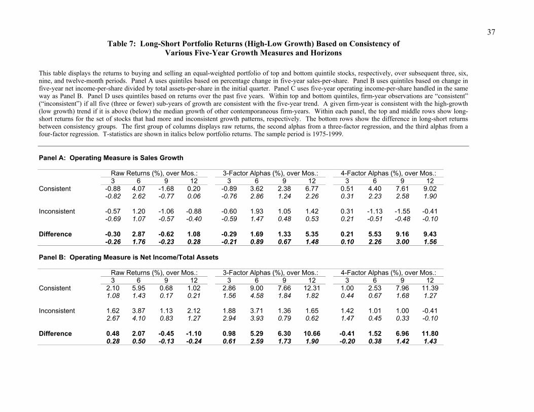
37

Table 7: Long-Short Portfolio Returns (High-Low Growth) Based on Consistency of Various Five-Year Growth Measures and Horizons

This table displays the returns to buying and selling an equal-weighted portfolio of top and bottom quintile stocks, respectively, over subsequent three, six, nine, and twelve-month periods. Panel A uses quintiles based on percentage change in five-year sales-per-share. Panel B uses quintiles based on change in five-year net income-per-share divided by total assets-per-share in the initial quarter. Panel C uses five-year operating income-per-share handled in the same way as Panel B. Panel D uses quintiles based on returns over the past five years. Within top and bottom quintiles, firm-year observations are “consistent” (“inconsistent”) if all five (three or fewer) sub-years of growth are consistent with the five-year trend. A given firm-year is consistent with the high-growth (low growth) trend if it is above (below) the median growth of other contemporaneous firm-years. Within each panel, the top and middle rows show long-short returns for the set of stocks that had more and inconsistent growth patterns, respectively. The bottom rows show the difference in long-short returns between consistency groups. The first group of columns displays raw returns, the second alphas from a three-factor regression, and the third alphas from a four-factor regression. T-statistics are shown in italics below portfolio returns. The sample period is 1975-1999. Panel A: Operating Measure is Sales Growth Raw Returns (%), over Mos.: 3-Factor Alphas (%), over Mos.: 4-Factor Alphas (%), over Mos.: 3 6 9 12 3 6 9 12 3 6 9 12 Consistent -0.88 4.07 -1.68 0.20 -0.89 3.62 2.38 6.77 0.51 4.40 7.61 9.02 -0.82 2.62 -0.77 0.06 -0.76 2.86 1.24 2.26 0.31 2.23 2.58 1.90 Inconsistent -0.57 1.20 -1.06 -0.88 -0.60 1.93 1.05 1.42 0.31 -1.13 -1.55 -0.41 -0.69 1.07 -0.57 -0.40 -0.59 1.47 0.48 0.53 0.21 -0.51 -0.48 -0.10 Difference -0.30 2.87 -0.62 1.08 -0.29 1.69 1.33 5.35 0.21 5.53 9.16 9.43 -0.26 1.76 -0.23 0.28 -0.21 0.89 0.67 1.48 0.10 2.26 3.00 1.56

Panel B: Operating Measure is Net Income/Total Assets Raw Returns (%), over Mos.: 3-Factor Alphas (%), over Mos.: 4-Factor Alphas (%), over Mos.: 3 6 9 12 3 6 9 12 3 6 9 12 Consistent 2.10 5.95 0.68 1.02 2.86 9.00 7.66 12.31 1.00 2.53 7.96 11.39 1.08 1.43 0.17 0.21 1.56 4.58 1.84 1.82 0.44 0.67 1.68 1.27 Inconsistent 1.62 3.87 1.13 2.12 1.88 3.71 1.36 1.65 1.42 1.01 1.00 -0.41 2.67 4.10 0.83 1.27 2.94 3.93 0.79 0.62 1.47 0.45 0.33 -0.10 Difference 0.48 2.07 -0.45 -1.10 0.98 5.29 6.30 10.66 -0.41 1.52 6.96 11.80 0.28 0.50 -0.13 -0.24 0.61 2.59 1.73 1.90 -0.20 0.38 1.42 1.43

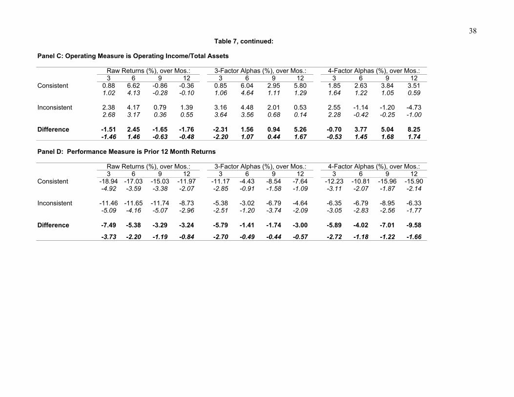
38

Table 7, continued: Panel C: Operating Measure is Operating Income/Total Assets Raw Returns (%), over Mos.: 3-Factor Alphas (%), over Mos.: 4-Factor Alphas (%), over Mos.: 3 6 9 12 3 6 9 12 3 6 9 12 Consistent 0.88 6.62 -0.86 -0.36 0.85 6.04 2.95 5.80 1.85 2.63 3.84 3.51 1.02 4.13 -0.28 -0.10 1.06 4.64 1.11 1.29 1.64 1.22 1.05 0.59 Inconsistent 2.38 4.17 0.79 1.39 3.16 4.48 2.01 0.53 2.55 -1.14 -1.20 -4.73 2.68 3.17 0.36 0.55 3.64 3.56 0.68 0.14 2.28 -0.42 -0.25 -1.00 Difference -1.51 2.45 -1.65 -1.76 -2.31 1.56 0.94 5.26 -0.70 3.77 5.04 8.25 -1.46 1.46 -0.63 -0.48 -2.20 1.07 0.44 1.67 -0.53 1.45 1.68 1.74 Panel D: Performance Measure is Prior 12 Month Returns Raw Returns (%), over Mos.: 3-Factor Alphas (%), over Mos.: 4-Factor Alphas (%), over Mos.: 3 6 9 12 3 6 9 12 3 6 9 12 Consistent -18.94 -17.03 -15.03 -11.97 -11.17 -4.43 -8.54 -7.64 -12.23 -10.81 -15.96 -15.90 -4.92 -3.59 -3.38 -2.07 -2.85 -0.91 -1.58 -1.09 -3.11 -2.07 -1.87 -2.14 Inconsistent -11.46 -11.65 -11.74 -8.73 -5.38 -3.02 -6.79 -4.64 -6.35 -6.79 -8.95 -6.33 -5.09 -4.16 -5.07 -2.96 -2.51 -1.20 -3.74 -2.09 -3.05 -2.83 -2.56 -1.77 Difference -7.49 -5.38 -3.29 -3.24 -5.79 -1.41 -1.74 -3.00 -5.89 -4.02 -7.01 -9.58 -3.73 -2.20 -1.19 -0.84 -2.70 -0.49 -0.44 -0.57 -2.72 -1.18 -1.22 -1.66

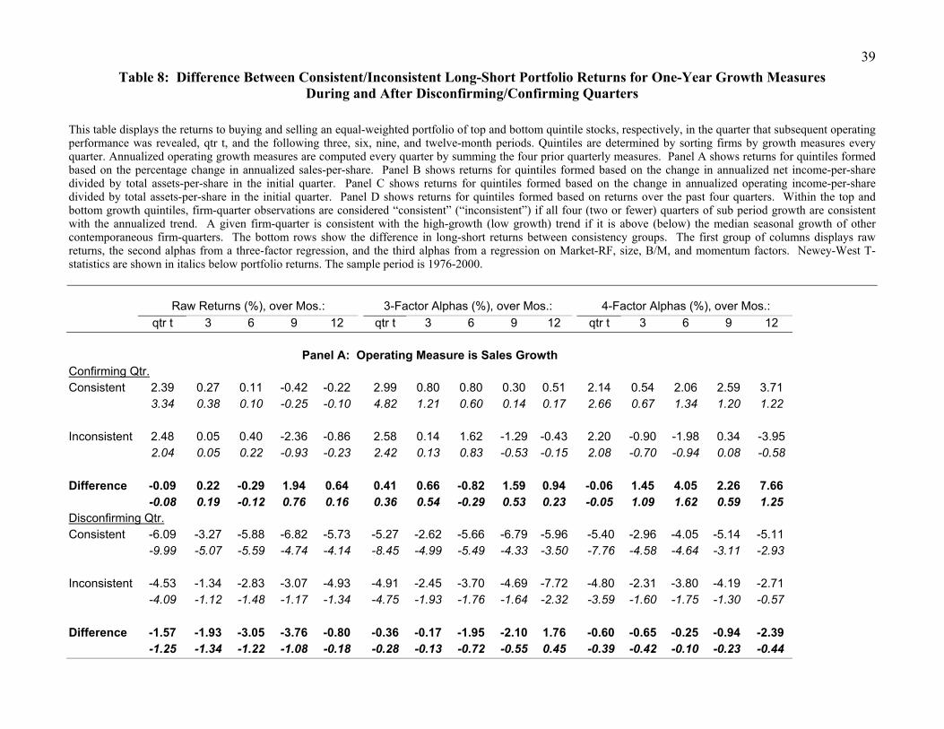
39

Table 8: Difference Between Consistent/Inconsistent Long-Short Portfolio Returns for One-Year Growth Measures During and After Disconfirming/Confirming Quarters

This table displays the returns to buying and selling an equal-weighted portfolio of top and bottom quintile stocks, respectively, in the quarter that subsequent operating performance was revealed, qtr t, and the following three, six, nine, and twelve-month periods. Quintiles are determined by sorting firms by growth measures every quarter. Annualized operating growth measures are computed every quarter by summing the four prior quarterly measures. Panel A shows returns for quintiles formed based on the percentage change in annualized sales-per-share. Panel B shows returns for quintiles formed based on the change in annualized net income-per-share divided by total assets-per-share in the initial quarter. Panel C shows returns for quintiles formed based on the change in annualized operating income-per-share divided by total assets-per-share in the initial quarter. Panel D shows returns for quintiles formed based on returns over the past four quarters. Within the top and bottom growth quintiles, firm-quarter observations are considered “consistent” (“inconsistent”) if all four (two or fewer) quarters of sub period growth are consistent with the annualized trend. A given firm-quarter is consistent with the high-growth (low growth) trend if it is above (below) the median seasonal growth of other contemporaneous firm-quarters. The bottom rows show the difference in long-short returns between consistency groups. The first group of columns displays raw returns, the second alphas from a three-factor regression, and the third alphas from a regression on Market-RF, size, B/M, and momentum factors. Newey-West T-statistics are shown in italics below portfolio returns. The sample period is 1976-2000. Raw Returns (%), over Mos.: 3-Factor Alphas (%), over Mos.: 4-Factor Alphas (%), over Mos.: qtr t 3 6 9 12 qtr t 3 6 9 12 qtr t 3 6 9 12

Panel A: Operating Measure is Sales Growth Confirming Qtr. Consistent 2.39 0.27 0.11 -0.42 -0.22 2.99 0.80 0.80 0.30 0.51 2.14 0.54 2.06 2.59 3.71 3.34 0.38 0.10 -0.25 -0.10 4.82 1.21 0.60 0.14 0.17 2.66 0.67 1.34 1.20 1.22 Inconsistent 2.48 0.05 0.40 -2.36 -0.86 2.58 0.14 1.62 -1.29 -0.43 2.20 -0.90 -1.98 0.34 -3.95 2.04 0.05 0.22 -0.93 -0.23 2.42 0.13 0.83 -0.53 -0.15 2.08 -0.70 -0.94 0.08 -0.58 Difference -0.09 0.22 -0.29 1.94 0.64 0.41 0.66 -0.82 1.59 0.94 -0.06 1.45 4.05 2.26 7.66 -0.08 0.19 -0.12 0.76 0.16 0.36 0.54 -0.29 0.53 0.23 -0.05 1.09 1.62 0.59 1.25 Disconfirming Qtr. Consistent -6.09 -3.27 -5.88 -6.82 -5.73 -5.27 -2.62 -5.66 -6.79 -5.96 -5.40 -2.96 -4.05 -5.14 -5.11 -9.99 -5.07 -5.59 -4.74 -4.14 -8.45 -4.99 -5.49 -4.33 -3.50 -7.76 -4.58 -4.64 -3.11 -2.93 Inconsistent -4.53 -1.34 -2.83 -3.07 -4.93 -4.91 -2.45 -3.70 -4.69 -7.72 -4.80 -2.31 -3.80 -4.19 -2.71 -4.09 -1.12 -1.48 -1.17 -1.34 -4.75 -1.93 -1.76 -1.64 -2.32 -3.59 -1.60 -1.75 -1.30 -0.57 Difference -1.57 -1.93 -3.05 -3.76 -0.80 -0.36 -0.17 -1.95 -2.10 1.76 -0.60 -0.65 -0.25 -0.94 -2.39 -1.25 -1.34 -1.22 -1.08 -0.18 -0.28 -0.13 -0.72 -0.55 0.45 -0.39 -0.42 -0.10 -0.23 -0.44

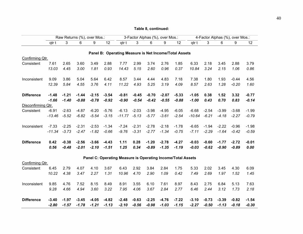
40

Table 8, continued:

Raw Returns (%), over Mos.: 3-Factor Alphas (%), over Mos.: 4-Factor Alphas (%), over Mos.: qtr t 3 6 9 12 qtr t 3 6 9 12 qtr t 3 6 9 12

Panel B: Operating Measure is Net Income/Total Assets Confirming Qtr. Consistent 7.61 2.65 3.60 3.49 2.88 7.77 2.99 3.74 2.76 1.85 6.33 2.18 3.45 2.88 3.79 13.03 4.45 3.00 1.81 0.93 14.43 5.15 2.60 0.96 0.37 10.84 3.24 2.15 1.06 0.86 Inconsistent 9.09 3.86 5.04 5.64 6.42 8.57 3.44 4.44 4.83 7.18 7.38 1.80 1.93 -0.44 4.56 12.39 5.84 4.55 3.76 4.11 11.22 4.93 5.25 3.19 4.09 8.57 2.63 1.28 -0.20 1.60 Difference -1.48 -1.21 -1.44 -2.15 -3.54 -0.81 -0.45 -0.70 -2.07 -5.33 -1.05 0.38 1.52 3.32 -0.77 -1.66 -1.40 -0.88 -0.78 -0.92 -0.90 -0.54 -0.42 -0.55 -0.88 -1.00 0.43 0.70 0.83 -0.14 Disconfirming Qtr. Consistent -6.91 -2.63 -4.87 -6.20 -5.76 -6.13 -2.03 -3.98 -4.95 -6.05 -6.68 -2.54 -3.99 -3.68 -1.99 -13.46 -5.52 -6.82 -5.54 -3.15 -11.77 -5.13 -5.77 -3.61 -2.54 -10.64 -6.21 -4.18 -2.27 -0.79 Inconsistent -7.33 -2.25 -2.31 -2.53 -1.34 -7.24 -2.31 -2.78 -2.18 -1.78 -6.65 -1.94 -2.22 -0.96 -1.98 -11.34 -3.73 -2.47 -1.82 -0.66 -9.76 -3.31 -2.77 -1.34 -0.75 -7.11 -2.29 -1.64 -0.42 -0.59 Difference 0.42 -0.38 -2.56 -3.66 -4.43 1.11 0.28 -1.20 -2.78 -4.27 -0.03 -0.60 -1.77 -2.72 -0.01 0.56 -0.48 -2.01 -2.10 -1.51 1.25 0.34 -0.89 -1.35 -1.19 -0.03 -0.62 -0.90 -0.89 0.00

Panel C: Operating Measure is Operating Income/Total Assets Confirming Qtr. Consistent 6.45 2.79 4.07 4.10 3.67 6.43 2.92 3.84 2.84 1.75 5.33 2.02 3.45 4.30 6.09 10.22 4.38 3.47 2.27 1.31 10.96 4.70 2.90 1.09 0.42 7.49 2.69 1.97 1.52 1.45 Inconsistent 9.85 4.76 7.52 8.15 8.49 8.91 3.55 6.10 7.61 8.97 8.43 2.75 6.84 5.13 7.63 9.28 4.66 4.94 3.60 3.22 7.95 4.06 3.67 2.84 2.77 6.46 2.44 3.12 1.73 2.18 Difference -3.40 -1.97 -3.45 -4.05 -4.82 -2.48 -0.63 -2.25 -4.76 -7.22 -3.10 -0.73 -3.39 -0.82 -1.54 -2.80 -1.57 -1.78 -1.21 -1.13 -2.10 -0.56 -0.98 -1.03 -1.15 -2.27 -0.50 -1.13 -0.18 -0.30

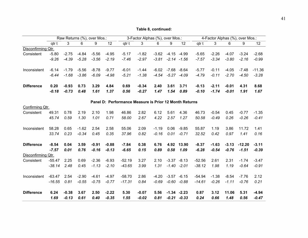
41

Table 8, continued:

Raw Returns (%), over Mos.: 3-Factor Alphas (%), over Mos.: 4-Factor Alphas (%), over Mos.: qtr t 3 6 9 12 qtr t 3 6 9 12 qtr t 3 6 9 12 Disconfirming Qtr. Consistent -5.80 -2.75 -4.84 -5.56 -4.95 -5.17 -1.82 -3.62 -4.15 -4.99 -5.65 -2.26 -4.07 -3.24 -2.68 -9.26 -4.39 -5.28 -3.56 -2.19 -7.46 -2.97 -3.81 -2.14 -1.56 -7.57 -3.34 -3.80 -2.16 -0.99 Inconsistent -6.14 -1.79 -5.56 -8.78 -9.77 -6.01 -1.44 -6.02 -7.68 -8.64 -5.77 -0.11 -4.05 -7.48 -11.36 -6.44 -1.68 -3.86 -6.09 -4.98 -5.21 -1.38 -4.54 -5.27 -4.09 -4.79 -0.11 -2.70 -4.50 -3.28 Difference 0.20 -0.93 0.73 3.29 4.84 0.69 -0.34 2.40 3.61 3.71 -0.13 -2.11 -0.01 4.31 8.68 -0.18 -0.73 0.48 1.61 1.37 0.56 -0.27 1.47 1.54 0.89 -0.10 -1.74 -0.01 1.91 1.67

Panel D: Performance Measure is Prior 12 Month Returns Confirming Qtr. Consistent 49.31 0.78 2.19 2.10 1.98 46.86 2.82 6.12 5.61 4.36 46.73 -0.54 0.45 -0.77 -1.35 45.74 0.59 1.30 1.01 0.71 58.00 2.67 4.22 2.57 1.27 50.58 -0.49 0.26 -0.26 -0.41 Inconsistent 58.28 0.65 -1.62 2.54 2.58 55.06 2.09 -1.19 0.06 -9.85 55.87 1.19 3.86 11.72 1.41 33.74 0.23 -0.34 0.45 0.35 37.96 0.82 -0.16 0.01 -0.71 32.52 0.42 0.97 1.41 0.16 Difference -8.54 0.04 3.59 -0.91 -0.88 -7.84 0.38 6.76 4.92 13.90 -8.37 -1.63 -3.13 -12.20 -3.11 -7.57 0.01 0.76 -0.16 -0.13 -6.65 0.15 0.89 0.58 1.09 -6.28 -0.54 -0.76 -1.51 -0.39 Disconfirming Qtr. Consistent -55.47 2.25 0.69 -2.36 -6.93 -52.19 3.27 2.10 -3.37 -8.13 -52.56 2.61 2.31 -1.74 -3.47 -38.14 2.48 0.45 -1.13 -2.10 -43.65 3.99 1.31 -1.40 -2.01 -38.12 1.98 1.19 -0.64 -0.91 Inconsistent -63.47 2.54 -2.90 -4.61 -4.97 -58.70 2.86 -4.20 -3.57 -6.15 -54.94 -1.38 -8.54 -7.76 2.12 -16.55 0.81 -0.55 -0.75 -0.77 -17.31 0.84 -0.69 -0.60 -0.88 -14.61 -0.26 -1.11 -0.76 0.21 Difference 6.24 -0.38 3.67 2.50 -2.22 5.30 -0.07 5.56 -1.34 -2.23 0.87 3.12 11.06 5.31 -4.94 1.69 -0.13 0.61 0.40 -0.35 1.55 -0.02 0.81 -0.21 -0.33 0.24 0.66 1.48 0.56 -0.47

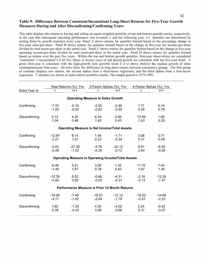
42

Table 9: Difference Between Consistent/Inconsistent Long-Short Returns for Five-Year Growth Measures During and After Disconfirming/Confirming Years This table displays the returns to buying and selling an equal-weighted portfolio of top and bottom quintile stocks, respectively, in the year that subsequent operating performance was revealed, t, and the following year, t+1. Quintiles are determined by sorting firms by growth measures every year. Panel A shows returns for quintiles formed based on the percentage change in five-year sales-per-share. Panel B shows returns for quintiles formed based on the change in five-year net income-per-share divided by total assets-per-share in the initial year. Panel C shows returns for quintiles formed based on the change in five-year operating income-per-share divided by total assets-per-share in the initial year. Panel D shows returns for quintiles formed based on returns over the past five years. Within the top and bottom growth quintiles, firm-year observations are considered “consistent” (“inconsistent”) if all five (three or fewer) years of sub period growth are consistent with the five-year trend. A given firm-year is consistent with the high-growth (low growth) trend if it is above (below) the median growth of other contemporaneous firm-years. All rows show the difference in long-short returns between consistency groups. The first group of columns displays raw returns, the second alphas from a three-factor regression, and the third alphas from a four-factor regression. T-statistics are shown in italics below portfolio returns. The sample period is 1975-1999. Raw Returns (%), Yrs: 3-Factor Alphas (%), Yrs: 4-Factor Alphas (%), Yrs:Extra Year is: t t+1 t t+1 t t+1

Operating Measure is Sales Growth Confirming -7.70 -0.10 -2.55 -2.46 1.71 5.14 -1.83 -0.02 -0.63 -0.50 0.26 0.78 Disconfirming 5.12 4.25 8.30 2.06 13.59 1.80 1.04 0.89 1.83 0.43 1.93 0.29

Operating Measure is Net Income/Total Assets

Confirming -12.97 8.14 1.54 -1.71 3.08 0.71 -2.27 1.91 0.23 -0.34 0.31 0.08 Disconfirming -3.43 -27.36 -4.78 -22.12 9.61 -6.50 -0.28 -1.53 -0.28 -0.72 0.60 -0.26

Operating Measure is Operating Income/Total Assets Confirming -6.46 5.21 3.36 1.39 11.70 7.44 -1.45 1.67 0.76 0.43 1.87 1.45 Disconfirming -12.39 8.52 -0.66 -4.31 -2.16 -12.28 -0.95 0.83 -0.05 -0.31 -0.13 -1.47

Performance Measure is Prior 12 Month Returns Confirming -16.26 -7.40 -18.51 -12.12 -16.52 -14.69 -4.11 -1.62 -2.94 -1.79 -3.53 -2.23 Disconfirming 1.82 -1.39 4.05 -4.02 2.24 -0.42 0.38 -0.32 0.96 -0.66 0.31 -0.07