LAND AND WATER

Test of WRF physics

schemes for Project 6 of the

Victorian Climate Initiative An outline of selected physical parameterisation schemes and other runtime options

Marie Ekström 8 August 2014

ii | P a g e

CSIRO Land and Water Flagship

CSIRO initiated the National Research Flagships to address Australia’s major research challenges and opportunities. They apply large scale, long term, multidisciplinary science and aim for widespread adoption of solutions.

The Land and Water Flagship provides the science to underpin Australia’s economic, social and environmental prosperity through stewardship of land and water resources ecosystems, and urban areas. For more information about the Flagship visit www.csiro.au/LWF

Citation

Ekström M (2014) Test of WRF physics schemes for Project 6 of the Victorian Climate Initiative; an outline of selected physical parameterisation schemes and other runtime options. CSIRO Land and Water Flagship, Australia.

Copyright and disclaimer

© 2014 CSIRO To the extent permitted by law, all rights are reserved and no part of this publication covered by copyright may be reproduced or copied in any form or by any means except with the written permission of CSIRO.

Important disclaimer

CSIRO advises that the information contained in this publication comprises general statements based on scientific research. The reader is advised and needs to be aware that such information may be incomplete or unable to be used in any specific situation. No reliance or actions must therefore be made on that information without seeking prior expert professional, scientific and technical advice. To the extent permitted by law, CSIRO (including its employees and consultants) excludes all liability to any person for any consequences, including but not limited to all losses, damages, costs, expenses and any other compensation, arising directly or indirectly from using this publication (in part or in whole) and any information or material contained in it.

Foreword

The Victorian Climate Initiative (VicCI) is a 3 year State funded initiative involving the Australian Bureau of Meteorology and the CSIRO. With a focus on the State of Victoria, research activities split into 7 projects, aim to assess trends and patterns in the variability of regional drivers of rainfall in current and plausible future climates.

This technical report, details choices about physical parameterisation schemes, choices about dynamical settings and other runtime options, as used in the first set of climate simulation experiments conducted for Project 6 of the Victorian Climate Initiative ‘Convection-resolving dynamical downscaling’. The overall aim of Project 6 is to assess the potential added value of very high resolution dynamical downscaling for the purpose of better resolving the temporal and spatial characteristics of regional rainfall patterns. The difference being that in very high climate simulations, convective rainfall is resolved by the model rather than being parameterised as a sub-grid resolution process.

2 | P a g e

Contents

Foreword ............................................................................................................................................................ 1

Acknowledgments .............................................................................................................................................. 5

Executive summary............................................................................................................................................. 6

1 Introduction .......................................................................................................................................... 7

2 Regional climate model setup and input data ...................................................................................... 8

2.1 Physics schemes .......................................................................................................................... 8

2.2 Physics ensemble specification ................................................................................................. 12

2.3 Other runtime options .............................................................................................................. 13

2.4 Forcing data .............................................................................................................................. 13

3 Case study selection ............................................................................................................................ 14

4 Evaluation of WRF rainfall output ....................................................................................................... 21

4.1 Skill metrics ............................................................................................................................... 21

4.2 Evaluation of simulated rainfall for domain d02 ...................................................................... 23

4.3 Evaluation of simulated rainfall for domain d03 ...................................................................... 27

5 Summary ............................................................................................................................................. 31

Appendix A Parameter file ‘namelist.input’ ................................................................................................. 32

Appendix B Vtable for WRF pre-processor: Vtable.ERA-interim.pl ............................................................. 35

References ........................................................................................................................................................ 36

Figures Figure 1 Map showing the extent of radar coverage for central Victoria (stippled areas indicate areas outside the radar range) ................................................................................................................................... 14

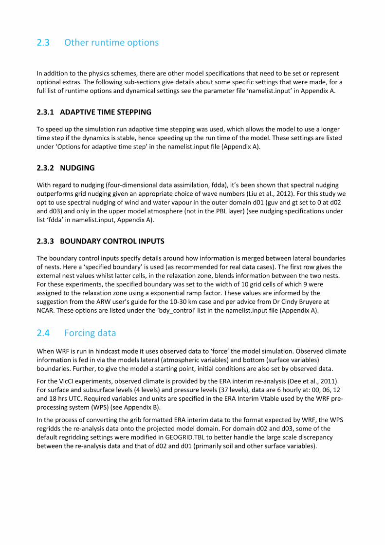
Figure 2 Daily rainfall total maps [mm] for 4th and 5th of September (top row panels) and 13th to 16th of October 2010 (mid and bottom panels). Maps were generated using the BoM online archive for daily rainfall ............................................................................................................................................................... 16

Figure 3 Monthly rainfall total maps [mm] for November 2010 to February 2011 ......................................... 17

Figure 4 Mean sea level pressure analysis (00 UTC) from the top) 15th August 2010, middle) 15th October 2010 and bottom) 5th of February 2011 ........................................................................................................... 18

Figure 5 Spatial extent of the three domains: d01, d02 and d03 (in decreasing size). The red dots denote the outer boundary and the black dots outline the domain excluding the relaxation zone ........................... 20

Figure 6 Extent of the innermost domain d03, with relaxation boundary removed ....................................... 20

Figure 7 Temporal evolution of rainfall in domain d02 (case study 1) displayed as grid total rainfall (mm) for WRF members (blue) and AWAP (orange) in panel a, and as bias (difference in grid total rainfall, WRF-AWAP) in panel b ..................................................................................................................................... 24

Figure 8 Simple skill scores for domain d02. Upper panel shows ensemble members N1-N4 (using pbl scheme MYNN) and lower panel shows ensemble members N6-N9 (using pbl scheme YSU) ........................ 25

Figure 9 FSS for domain d02. Upper panel shows ensemble members N1-N4 (using pbl scheme MYNN) and lower panel shows ensemble members N6-N9 (using pbl scheme YSU). Each group of box plots show the FSS using a neighbourhood length of 1, 3, 5 and 11 grid cells. .................................................................. 26

Figure 10 Temporal evolution of rainfall in domain d03 (case study 1) displayed as grid total rainfall (mm) for WRF members (blue) and AWAP (orange) in panel a, and as bias (difference in grid total rainfall, WRF-AWAP) in panel b ........................................................................................................................ 28

Figure 11 Simple skill scores for domain d03. Upper panel shows ensemble members N1-N4 (using pbl scheme MYNN) and lower panel shows ensemble members N6-N9 (using pbl scheme YSU). ....................... 28

Figure 12 FSS for domain d03. Upper panel shows ensemble members N1-N4 (using pbl scheme MYNN) and lower panel shows ensemble members N6-N9 (using pbl scheme YSU). Each group of box plots show the FSS using a neighbourhood length of 1, 3, 5 and 11 grid cells. .................................................................. 29

Tables Table 1 Proposed mp schemes for domain d01, d02 and d03. The number in brackets denotes the assigned number to use in the namelist.input file ............................................................................................. 9

Table 2 Proposed long and shortwave radiation schemes for domain d01, d02 and d03 and update frequency. The number in brackets denotes the assigned number to use in the namelist.input file ............. 11

Table 3 Proposed pbl schemes for domain d01, d02 and d03. The number in brackets denotes the assigned number to use in the namelist.input file ........................................................................................... 11

Table 4 Proposed surface physics schemes for domain d01, d02 and d03. The number in brackets denotes the assigned number to use in the namelist.input file ....................................................................... 11

Table 5 List of physics options associated with each ensemble member N1-N10........................................... 12

4 | P a g e

Table 6 Contingency table for simple verification metrics ............................................................................... 22

Table 7 For domain d02 and each simple skill score, the median (50th percentile) and the lower and upper quantile (25th and 75th percentile) within brackets ............................................................................... 25

Table 8 For domain d02 and for each FSS (neighbourhood length of: 1, 3, 5 and 11 grid cells), the median (50th percentile) and the lower and upper quantile (25th and 75th percentile) within brackets ...................... 26

Table 9 For domain d03 and each simple skill score, the median (50th percentile) and the lower and upper quantile (25th and 75th percentile) within brackets ............................................................................... 29

Table 10 For domain d03 and for each FSS (neighbourhood length of: 1, 3, 5 and 11 grid cells), the median (50th percentile) and the lower and upper quantile (25th and 75th percentile) within brackets ......... 30

Acknowledgments

The Victorian Climate Initiative (VicCI) is funded by the State of Victoria through the Department of Environment and Primary Industries (DEPI). The author would like to acknowledge the help of John Gallant and Jenet Austin of the CSIRO in formatting the 9s DEM used for these WRF simulations.

6 | P a g e

Executive summary

The Advanced Research Weather and Research Forecasting (WRF) modelling system is a community supported model hosted at the NCAR Mesoscale and Microscale Meteorology division. This model will be used to assess the value of very high resolution (<3km) versus high resolution (~10km) dynamical downscaling for the purpose of better representation of spatial and temporal characteristics of rainfall. Improvements should lead to more informative estimates of regional runoff in a climate change impact context.

WRF is highly configurable, and prior to conducting climate change experiments it is necessary to test the suitability of application relevant physics options. Based on user guidance and peer-review literature, initial testing in Project 6 identified 10 ensemble members, focusing on the sensitivity of rainfall to the microphysics schemes (that generates the grid scale rainfall), in combination with two different planetary boundary schemes.

Three case studies were proposed for the comparison, each a two-week simulation over the same spatial domain. The latter was selected in consultation with stakeholders and research partners, considering (a) criteria for selecting robust domains and (b) limitations imposed by computing resources (storage and time). The chosen structure is a nested configuration (50 km/10 km/ 2km) with the innermost grid focusing on a region about 450 by 600km stretching from just east of the Great dividing range towards east of (but not including) the Grampians national park. In a north to south direction, the innermost domain encompass’ the southern coastline and the state boundary towards New South Wales.

The three temporal domains represent winter, spring and summer, each encompassing a simulation period of 15 days of which one day is removed for model spin-up, the three 14-day case study periods are: 8th to 21st August 2010, 6th to 19th of October 2010 and 31st January to 13th of February 2011 . The selection of case study periods was guided by a discussion with stakeholders, focussing on a multi-month period wherein Victoria experienced repeated extensive flooding. Within this period, three two-week periods were selected based on recorded flooding events and a visual examination of synoptic mean sea level pressure charts and daily rainfall maps.

By the end of the first project year, model simulations for the first case study is completed, with two to follow. Initial assessment of model skill is reported here for the two inner domains d02 (10 km resolution) and d03 (2km resolution) for the first case study (winter).

Simulations were assessed on their native grids to gridded observed rainfall data from the Australian Water Availability (AWAP) project using skill measures adapted for deterministic categorical forecasts, suitable for event based variables.

For domains d02 (10km) and d03 (2km), a somewhat better performance (as judged by the used metrics) was gained by simulations using microphysics scheme WDM6 in combination with the planetary boundary layer scheme MYNN.

Further research will compare model simulations on a single resolution to assess significant distributional differences in rainfall between d02 and d03 in comparison to observed data. Other simulated variables will also be assessed to determine suitability of the different ensemble members for future use within the Victorian Climate Initiative (VicCI).

1 Introduction

This is a technical document, reporting on the regional climate model (RCM) experiments conducted within the first year of Project 6 (Convection-resolving dynamical downscaling) of the Victorian Climate Initiative (VicCI).

VicCI is a 3 year projected funded by the State of Victoria through its Department of Environment and Primary Industries (DEPI), the Australian Bureau of Meteorology (BoM) and the CSIRO. The project is managed by BoM, with CSIRO subcontracted to lead two of the 7 projects aimed at assessing trends and patterns in the variability of regional drivers of rainfall in current and plausible future climates.

Project 6 is the one of the two projects lead by CSIRO and focuses on an assessment of the relative benefit of using very high spatial and temporal resolution downscaling that is convective permitting (<3km) compared to a less computationally expensive spatial resolution for the purpose of supporting water supply and demand climate change projections in Victoria. Of secondary interest is the ability of very high resolution RCM experiments to inform on high intensity rainfall relevant for climate change projections of future flooding. By the end of VicCI, Project 6 aim to provide guidance on whether the computational cost associated with the very high spatial resolution RCM is warranted from a water resource perspective.

The main motivation for this report is to document the model setup choices as well as other runtime options used for the VicCI experiments. Further, this document gives detail on the selection of the case studies used to test the model physics ensemble from which a smaller selection will be used (if time permitting) to conduct climate change impact studies within VicCI.

8 | P a g e

2 Regional climate model setup and input data

The downscaling experiment is conducted using the Weather and Research Forecasting (WRF) system version 3.5.1 (Skamarock and Klemp, 2008) with boundary and initial condition data from the ERA-Interim re-analysis data set (Dee et al., 2011).

The WRF is a community model system that supports two different dynamical cores, the Advanced Research WRF (ARW)1 hosted by the Mesoscale and Microscale Meteorology Division of the U.S. based National Center of Atmospheric Research (NCAR), and the WRF-NMM hosed by the Developmental Testbed Centre (DTC)2 . The ARW core is commonly the choice for regional climate downscaling applications and was the choice for VicCI.

For both cores, a variety of physics options are possible, reflecting the diverse nature of WRF’s application. Further, because it is a community supported model, user groups can introduce new physics schemes that after robust testing are included as viable options in the WRF modelling system. Consequently, for most parameter schemes, there are multiple options to choose from.

The diversity of physics parameter schemes allows the model to be used for different applications across a range of scales. However, on a practical level, the many choices can be a challenge to the user who may be faced with a range of schemes that on their theoretical merits appears more or less equal; so there is no obvious ‘right’ choice. In these instances, it would be prudent to conduct preliminary tests to see what configuration works best for the intended application and geographical region.

The WRF simulations for VicCI can to some extent draw upon tests of physics schemes conducted for the NSW/ACT Regional Climate Modelling (NARCliM) project, where a 36 member ensemble was run for a range of East Coast low events to identify robust model configurations (Evans et al., 2012). In many ways these experiments are comparable, as they: focus on a similar geographical region, are done as a pre-curser to dynamical downscaling of Global Climate Model output and with a particular interest in accurately representing regional rainfall. However, a direct implementation of the Evans et al. (2012) results for VicCI is not appropriate, as the VicCI experiments run at a higher resolution, which puts emphasis on a somewhat different set of parameter schemes, compared to those of primary interest in Evans et al. (2012).

In addition to physics schemes, the model setup involves other decisions with regard to dynamics and other runtime options. All the user defined settings are communicated to the model via a parameter file, ‘namelist.input’ (Appendix A). This chapter gives details on physics settings, the ensemble configuration for VicCI and the input data used to test the physics ensemble.

2.1 Physics schemes

In this section, the choices of physics schemes for the VicCI experiments are detailed and justified. These choices form the basis for selecting the model configurations to be tested for subsequent VicCI downscaling experiments. Guidance on parameter settings are given in the ARW user’s guide (NCAR, 2013), as well as in online tutorials on the operation of WRF3. Additional guidance can be derived from the peer-review literature, in particular work that focus on the Australian region e.g. Evans et al. (2012)

1 http://www.mmm.ucar.edu/wrf/users/ 2 http://www.dtcenter.org/wrf-nmm/users/ 3 http://www.mmm.ucar.edu/wrf/OnLineTutorial/index.htm

2.1.1 MICROPHYSICS SCHEMES

The microphysic (mp) scheme mp_physics describes the physics of atmospheric heat and moisture fluxes and gives the surface resolved-scale rainfall. There are several mp schemes available for WRF reflecting its many usages, which can make selection difficult. In (Evans et al., 2012), the mp scheme was of less importance to the skill of the rainfall simulation in comparison to the planetary boundary layer (pbl) scheme and the cumulative (cu) rainfall scheme. However, given the focus on convective permitting rainfall here, the mp scheme requires careful consideration and could be a source of significant uncertainty.

The first consideration with regard to mp scheme involves whether to use single or double moment schemes; where single moment schemes predict mass (for individual hydrometeor species) using a parameterised distribution of particle size. In the double moment schemes, an additional prediction equation is included to estimate the number concentration per double moment species. The double moment schemes allows for additional processes, such as size sorting during fall-out to be resolved by the scheme. Hence, double moment schemes are more complex with potentially larger capability compared to single moment schemes at high spatial resolutions.

The ARW User’s guide propose the use of a double moment scheme (Thompson) for convective permitting (dx=1-4km) runs and a single moment scheme (WSM6) for regional climate cases (dx=10-30 km). It is noted that whilst resolving graupel is probably not necessary for schemes dx >10km, it should be considered when attempting to resolve individual updrafts, as ice content is important for rainfall. In the shortwave spectrum, less ice leads to more shortwave heating of the surface, more buoyancy and more implicit rain (Hong et al., 2004); where implicit clouds reduce or eliminate convective instability and produce rainfall (Molinari and Dudek, 1986). In the longwave spectrum, less ice implies less longwave heating, higher relative humidity and more explicit rain.

The WRF guide also suggests that the same mp scheme should be used in all domains if possible. For the first case study of Project 6 in VicCI, five setups are proposed testing all double moment types that also consider graupel. These are: the WRF double moment 6-class scheme (WDM6) (Lim and Hong, 2010), the Thompson scheme (Thompson et al., 2008), the Milbrandt scheme (Milbrandt and Yau, 2005), the Morrison scheme (Hong and Pan, 1996) and the NSSL scheme (Mansell et al., 2010) (Table 1).

Table 1 Proposed mp schemes for domain d01, d02 and d03. The number in brackets denotes the assigned number to use in the namelist.input file

D01 D02 D03

MP setup 1 WDM6 [16] WDM6 [16] WDM6 [16]

MP setup 2 Thompson [8] Thompson [8] Thompson [8]

MP setup 3 Milbrandt [9] Milbrandt [9] Milbrandt [9]

MP setup 4 Morrison [10] Morrison [10] Morrison [10]

MP setup 5 NSSL [17] NSSL [17] NSSL [17]

10 | P a g e

2.1.2 LONG AND SHORT WAVE RADIATION

The radiation schemes provide the atmospheric temperature tendency profile and estimates of surface radiative fluxes. Similar to the mp-schemes, long and short wave radiation schemes were noted as less relevant to WRF’s skill in simulating rainfall relative to the cu and pbl schemes in Evans et al. (2012) for southeast Australia. For this application, it is not obvious that radiation should play a larger role compared to that in Evans et al. (2012), though it is noted that radiation schemes interacts with the microphysics schemes via different mass variables. Hence, selected options are required to be compatible with choices of mp schemes. Further, the selected scheme needs to allow for time-varying emission concentrations in preparation for planned climate change runs.

Long wave

The long wave schemes compute clear-sky and cloud upward and downward radiation fluxes, where infra red (IR) radiation generally leads to cooling in clear air, stronger cooling at cloud tops and warming at the cloud base. There are seven schemes to choose from, where key differing properties are microphysics interaction (what mass variables are interacted with), method of representing cloud cover, and how to handle greenhouse gas (GHG) concentrations. Given the need to consider varying GHG concentrations two schemes that use constant, or no GHG concentration are immediately excluded. This leaves, RRTM, CAM and RRTMG of which only RRTM considers interactions with 5 mp mass variables (cloud water, rain, cloud ice, snow and graupel). RRTMG has interaction with 4 mp (excluding graupel) mass variables and CAM 3 mp (excluding rain and graupel) mass variables.

With regard to cloud treatment, RRTM uses simple cloud fraction of 1/0 whilst CAM and RRTMG uses a more advanced method based on RH. For the latter it is necessary to make assumptions about overlay and there may be multiple layers with varying fractions. The CAM and RRTMG methods use maximum-random overlap method (maximum for neighbouring cloudy layers and random for layers separated by clear air), though more sophisticated the maximum-random overlap can be sensitive to the vertical resolution unless the effects of cloud fraction and cloud emissivity are considered separately (Raisanen, 1998).

For the proposed case study, the RRTM (Mlawer et al., 1997) or RRTMG (Iacono et al., 2008) schemes are potential options for long wave radiation treatment.

Short wave

The shortwave schemes compute clear-sky and cloudy solar fluxes, and most consider downward as well as upward (reflected fluxes). The main effects are warming in clear sky and constituting an important component of the surface energy balance. Overall there are seven shortwave radiation schemes, to be matched up with corresponding long wave scheme.

Having eliminated all but two longwave radiation schemes, there are two possible options for shortwave scheme: Dudhia(Dudhia, 1989) and RRTMG (Iacono et al., 2008) (where the former is matched with RRTM). Noteworthy here is that the Dudhia scheme has no treatment of ozone, relevant to maintain a warm stratosphere (important for model tops above ~20 km (50hPa), further RRTMG has the potential to handle trace gases such as N20 and CH4. The handling of clouds is the same as that of the corresponding scheme in the longwave spectrum.

The ARW User’s guide recommends RRTMG for the 1-4 km case and CAM (nb 3) for the 10-30km case. For the increased ability to consider gaseous constituents in the atmosphere that could be important in a climate change context, the RRTMG scheme is chosen. The time step for the radiation update is recommended to be set at about 1 min per km resolution and unless 2-way nesting is used, each nest can have its own value. However, on the recommendation from WRF support we use the same interval for updates in each domain (here 10 min).

Table 2 Proposed long and shortwave radiation schemes for domain d01, d02 and d03 and update frequency. The number in brackets denotes the assigned number to use in the namelist.input file

D01 D02 D03

Ra_lw and Ra_sw RRTMG [4] RRTMG [4] RRTMG [4]

radt 10 min 10min 10min

2.1.3 MIXING OF SURFACE FLUXES INTO THE BOUNDARY LAYER

The mixing of surface fluxes into the boundary layers is governed by the surface physics scheme (sf_sfclay_physics), land surface model (LSM) scheme (sf_surface_physics) and the pbl scheme (bl_pbl_physics). The calling sequence of schemes starts with the surface layer, providing information about e.g. moisture and heat fluxes to the land surface (unless over water) and then the pbl scheme. Essentially there are two choices to be made as the pbl scheme is generally tied to a specific surface physics scheme. Hence the surface physics scheme depends on what pbl scheme is selected.

Numerous evaluations exists of WRF pbl schemes in the literature, and particular relevant paper for convection permitting cases were conducted by (Coniglio et al., 2013), comparing three ‘local’ schemes and two ‘non-local’ schemes; where local and non-local refers to the closure schemes for the vertical mixing, where local schemes consider only adjacent fields for solving equations for unknown variables. Low biased results were given by the local scheme Mellor-Yamada Nakanishi and Niino Level 2.5 (MYNN WRF option 5). Other more general advice from the WRF user website, suggest to go with established tested PBL schemes such as the local scheme Mellor-Yamada-Janjic (MYJ) or the non-local closure scheme Yonsei University (YSU) scheme. We note that the ARW User’s guide propose the YSU scheme for the 10-30 km case and the MYJ scheme for the 1-4 km case. Here, we propose to use MYNN (local) (Nakanishi and Niino, 2006) and contrast it with YSU (non-local)(Hong et al., 2006).

Table 3 Proposed pbl schemes for domain d01, d02 and d03. The number in brackets denotes the assigned number to use in the namelist.input file

D01 D02 D03

PBL option 1 MYNN [5] MYNN [5] MYNN [5]

PBL option 2 YSU [1] YSU [1] YSU [1]

From these choices of pbl schemes follows that MYNN can be combined with three different surface physics schemes, whilst YSU can only be combined with one scheme; MM5 is common to both (Table 4). For this case study, MM5 is chosen so to reduce the number of varying schemes (Table 4).

Table 4 Proposed surface physics schemes for domain d01, d02 and d03. The number in brackets denotes the assigned number to use in the namelist.input file

POSSIBLE OPTIONS D01 D02 D03

sf_sfclay_physics (for PBL option 1)

MM5 similarity [1], Janjic [2] or MYNN [5]

MM5

similarity [1]

MM5

similarity [1]

MM5

similarity [1]

sf_sfclay_physics (for PBL option 2)

MM5

similarity [1]

MM5

similarity [1]

MM5

similarity [1]

MM5

similarity [1]

12 | P a g e

The LSM handles soil moisture and soil temperature, as well as fluxes associated with vegetation cover (e.g., evapotranspiration and leaf effects). WRF has six different LSM options of various complexities. For this case study we are interested in a model of intermediate complexity, hence we select a tried and tested LSM, which also is the proposed scheme for 1-4km and 10-30km experiments, the Noah LSM (WRF option 2).

2.1.4 CUMULUS SCHEME

The convective scheme is used to re-distribute air in atmospheric column to account for non-resolved vertical (convective) fluxes. These schemes determine when to trigger convection and how fast the convection acts. For cumulus one scheme is used. Analysis in (Evans et al., 2012) showed that the combination of the pbl scheme YSU with radiation scheme RRTMG performed consistently bad when paired with the cu scheme Kain-Fritsch (KF). For this reason the second cu scheme tested in (Evans et al., 2012), the Betts-Miller-Janjic (BMJ) scheme is selected, as YSU and RRTMG are used in this experiment set-up.

Note that this scheme (WRF option 2) is only implemented in domain d01 and d02. The BMJ scheme is the only WRF cu scheme that is of an ‘adjustment type’ (rather than ‘mass-flux type’) by which values are relaxed towards a post-convective (mixed) sounding (Janjic, 2000, Janjic, 1994).

2.2 Physics ensemble specification

The physic settings identified as relevant for VicCI are summarised in Table 5, outlining the physics ensemble used for initial tests of WRF for VicCI. The ensemble tests five mp schemes in combination with two pbl schemes, giving a total of 10 ensemble members.

Table 5 List of physics options associated with each ensemble member N1-N10

NB PBL MP SURF_PHYS RA SW/LW LSM CU D01/D02

1 MYNN WDM6 MM5 RRTMG Noah BMJ

2 MYNN Thompson MM5 RRTMG Noah BMJ

3 MYNN Milbrandt MM5 RRTMG Noah BMJ

4 MYNN Morrison MM5 RRTMG Noah BMJ

5 MYNN NSSL MM5 RRTMG Noah BMJ

6 YSU WDM6 MM5 RRTMG Noah BMJ

7 YSU Thompson MM5 RRTMG Noah BMJ

8 YSU Milbrandt MM5 RRTMG Noah BMJ

9 YSU Morrison MM5 RRTMG Noah BMJ

10 YSU NSSL MM5 RRTMG Noah BMJ

2.3 Other runtime options

In addition to the physics schemes, there are other model specifications that need to be set or represent optional extras. The following sub-sections give details about some specific settings that were made, for a full list of runtime options and dynamical settings see the parameter file ‘namelist.input’ in Appendix A.

2.3.1 ADAPTIVE TIME STEPPING

To speed up the simulation run adaptive time stepping was used, which allows the model to use a longer time step if the dynamics is stable, hence speeding up the run time of the model. These settings are listed under ‘Options for adaptive time step’ in the namelist.input file (Appendix A).

2.3.2 NUDGING

With regard to nudging (four-dimensional data assimilation, fdda), it’s been shown that spectral nudging outperforms grid nudging given an appropriate choice of wave numbers (Liu et al., 2012). For this study we opt to use spectral nudging of wind and water vapour in the outer domain d01 (guv and gt set to 0 at d02 and d03) and only in the upper model atmosphere (not in the PBL layer) (see nudging specifications under list ‘fdda’ in namelist.input, Appendix A).

2.3.3 BOUNDARY CONTROL INPUTS

The boundary control inputs specify details around how information is merged between lateral boundaries of nests. Here a ‘specified boundary’ is used (as recommended for real data cases). The first row gives the external nest values whilst latter cells, in the relaxation zone, blends information between the two nests. For these experiments, the specified boundary was set to the width of 10 grid cells of which 9 were assigned to the relaxation zone using a exponential ramp factor. These values are informed by the suggestion from the ARW user’s guide for the 10-30 km case and per advice from Dr Cindy Bruyere at NCAR. These options are listed under the ‘bdy_control’ list in the namelist.input file (Appendix A).

2.4 Forcing data

When WRF is run in hindcast mode it uses observed data to ‘force’ the model simulation. Observed climate information is fed in via the models lateral (atmospheric variables) and bottom (surface variables) boundaries. Further, to give the model a starting point, initial conditions are also set by observed data.

For the VicCI experiments, observed climate is provided by the ERA interim re-analysis (Dee et al., 2011). For surface and subsurface levels (4 levels) and pressure levels (37 levels), data are 6 hourly at: 00, 06, 12 and 18 hrs UTC. Required variables and units are specified in the ERA Interim Vtable used by the WRF pre-processing system (WPS) (see Appendix B).

In the process of converting the grib formatted ERA interim data to the format expected by WRF, the WPS regridds the re-analysis data onto the projected model domain. For domain d02 and d03, some of the default regridding settings were modified in GEOGRID.TBL to better handle the large scale discrepancy between the re-analysis data and that of d02 and d01 (primarily soil and other surface variables).

14 | P a g e

3 Case study selection

Consultation with DEPI and BoM stakeholders in June 2013 suggested that it would be interesting to develop a case study on the 2010-2011 floods in Victoria focusing on the region north of Melbourne, encompassing the southernmost part of the Dividing range and its western slopes. The area would be about 200 by 200 km and should, if possible, overlap with the geographical extent of radar products for the region (see Figure 1).

Figure 1 Map showing the extent of radar coverage for central Victoria (stippled areas indicate areas outside the radar range)

Source: BoM

3.1.1 CASE STUDY PERIOD

A subsequent evaluation of rainfall events for this period was undertaken to assess a suitable time period for evaluation of the proposed physics schemes. Details on when severe flooding occurred were taken from the Final Report of the Review of the 2010-11 Flood Warnings and Response commissioned by the Victorian Government (Comrie, 2011). The report indicates the following dates of interest (as reported in the section The weather influence on the 2010-11 floods (Comrie, 2011:p.18-19)):

3rd September 2010 and onwards

12 October 2010 until the weekend

November and December 2010

9-15th January 2011

Early February 2011

Rainfall maps downloaded from the Australian Bureau of Meteorology’s (BoM) online archive of daily rainfall totals for Australia4 were then viewed for these dates and periods with regard to the spatial extent of rainfall patterns associated with the reported flood events.

For the 3-5th of September period, rainfall was most widespread on the 4th and 5th with regions of intense rainfall occurring in central Victoria and in the Mt Buller area (50-100 mm) on the 4th with somewhat higher totals in the Mt Buller are on the 5th (100-150 mm) (Figure 2a and b). For the mid-October period, the largest totals were recorded on the 15th and 16th of October, with widespread rainfall occurring on both days (Figure 2c and d). The heavier rainfall was observed in western Victoria and northeastern part of the Victorian Alps, particularly in the latter on the 16th of October (100-150 mm with smaller region experiencing excess of 150 mm).

4 http://www.bom.gov.au/jsp/awap/rain/archive.jsp?colour=colour&map=totals&period=daily&area=nat

16 | P a g e

Figure 2 Daily rainfall total maps [mm] for 4th

and 5th

of September (top row panels) and 13th

to 16th

of October 2010 (mid and

bottom panels). Maps were generated using the BoM online archive for daily rainfall

Source: Maps were generated using the BoM online archive for daily rainfall

A visual inspection of monthly rainfall totals for the November 2010 to February 2011 period suggests that rainfall in Victoria was generally in excess of 25 mm across the entire state with higher totals occurring foremost in the Victorian Alps (ranging from 200- 600 mm; larger totals in February) (Figure 3a-d). An exception is January when the higher rainfall totals are recorded for a central region between Ballarat and Bendigo (Figure 3c).

Figure 3 Monthly rainfall total maps [mm] for November 2010 to February 2011

Source: Maps were generated using the BoM online archive for daily rainfall

To test the physics ensembles selected for VicCI, three case studies are selected that represent different seasonal characteristics and takes into consideration the periods mentioned in the Victorian Government review of the 2010-11 Flood Warnings and Response. Each case study is 14 days (15 days simulation time, with first day removed as spin-up) and includes at least one major rainfall event. These are described below.

The first study represents a winter (or cold season: April to October) case (8th to 21st of August 2010) and pre-dates the flooding events mentioned above. During this period, rainfall occurs in conjunction with an upper level trough, and low level cold front associated with a low pressure system. This low pressure system develops on the 10th of August over Victoria and subsequently moves westward over the following couple of days. Further passages of cold fronts occur during the period 15-17th of August (Figure 4a), and again on the 19th-20th of August. Rainfall is associated with these passages.

The second study represents the shoulder season between the cold and warm (November to March) season and includes the heavy rainfall noted for mid-October: 6th to 19st October 2010. Notable rainfall events during this period occur in conjunction with a cold front passage on the 7th, an upper level trough on the 13th followed intense rainfall associated with a deep low centred over Victoria on the 15-16th (Figure 4b).

The third study represents the summer (or warm season) and encompasses the early February flooding events noted above: 31th January to 13th of February 2011). This period includes the passage of tropical cyclone Yasi, north of the study region; the passage enabling advection of a moist tropical air mass ahead of the, from the west, approaching prefrontal westerly trough (Figure 4c).

18 | P a g e

Figure 4 Mean sea level pressure analysis (00 UTC) from the top) 15th

August 2010, middle) 15th

October 2010 and bottom) 5

th of February 2011

Source: Maps are generated using the BoM online Analysis Chart Archive

3.1.2 CASE STUDY REGION

The experiment will make use of three nests to achieve the spatial resolution necessary for convective permitting runs (<3km). In a climate change context, downscaling is preformed so to resolve processes occurring on a sub-grid cell scale of the global climate models. Hence, the domain set up for the case study should, as far as possible, take into consideration physical reasons (unresolved geographical detail and dynamical responses) for why smaller scale processes may occur that are not well represented by GCMs. Further considerations are necessary with regard to the placement of boundaries, as these reflect a merger of two different physics schemes (in particular along the lateral boundaries of the outer nest). One would want to locate this blend of nests in an area where it will cause least disturbance to circulation patterns that influence the case study region and away from major topographical features.

For VicCI, we propose to place the outer (~50km grid) so that its relaxation band ends outside the coastline of Australia, with somewhat larger extension to the east and south. The first nest at 10 km resolution will be focused on southeast Australia covering the coastal border in the south and east with some extension into the ocean to resolve coastal circulation. The second nest (2km) is focused on an inland area, where the central low lands of Victoria rise towards the Alps in the eastern part of the state. This is the region that is covered by radar imagery and received heavy rainfall during the identified study period.

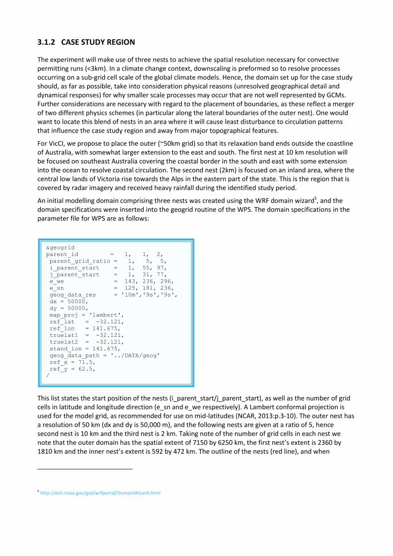
An initial modelling domain comprising three nests was created using the WRF domain wizard5, and the domain specifications were inserted into the geogrid routine of the WPS. The domain specifications in the parameter file for WPS are as follows:

This list states the start position of the nests (i_parent_start/j_parent_start), as well as the number of grid cells in latitude and longitude direction (e_sn and e_we respectively). A Lambert conformal projection is used for the model grid, as recommended for use on mid-latitudes (NCAR, 2013:p.3-10). The outer nest has a resolution of 50 km (dx and dy is 50,000 m), and the following nests are given at a ratio of 5, hence second nest is 10 km and the third nest is 2 km. Taking note of the number of grid cells in each nest we note that the outer domain has the spatial extent of 7150 by 6250 km, the first nest’s extent is 2360 by 1810 km and the inner nest’s extent is 592 by 472 km. The outline of the nests (red line), and when

5 http://esrl.noaa.gov/gsd/wrfportal/DomainWizard.html

&geogrid

parent_id = 1, 1, 2,

parent_grid_ratio = 1, 5, 5,

i_parent_start = 1, 55, 97,

j_parent_start = 1, 31, 77,

e_we = 143, 236, 296,

e_sn = 125, 181, 236,

geog_data_res = '10m','9s','9s',

dx = 50000,

dy = 50000,

map_proj = 'lambert',

ref_lat = -32.121,

ref_lon = 141.675,

truelat1 = -32.121,

truelat2 = -32.121,

stand_lon = 141.675,

geog_data_path = '../DATA/geog'

ref_x = 71.5,

ref_y = 62.5,

/

20 | P a g e

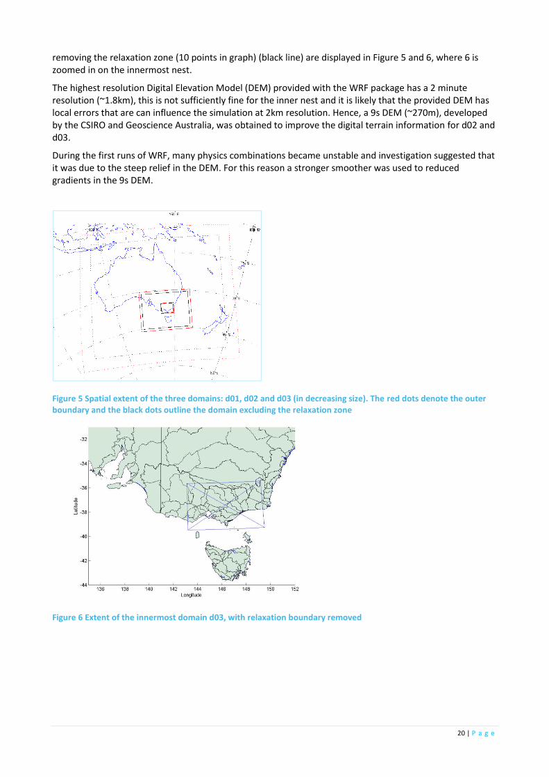
removing the relaxation zone (10 points in graph) (black line) are displayed in Figure 5 and 6, where 6 is zoomed in on the innermost nest.

The highest resolution Digital Elevation Model (DEM) provided with the WRF package has a 2 minute resolution (~1.8km), this is not sufficiently fine for the inner nest and it is likely that the provided DEM has local errors that are can influence the simulation at 2km resolution. Hence, a 9s DEM (~270m), developed by the CSIRO and Geoscience Australia, was obtained to improve the digital terrain information for d02 and d03.

During the first runs of WRF, many physics combinations became unstable and investigation suggested that it was due to the steep relief in the DEM. For this reason a stronger smoother was used to reduced gradients in the 9s DEM.

Figure 5 Spatial extent of the three domains: d01, d02 and d03 (in decreasing size). The red dots denote the outer boundary and the black dots outline the domain excluding the relaxation zone

Figure 6 Extent of the innermost domain d03, with relaxation boundary removed

4 Evaluation of WRF rainfall output

WRF runs on the high performance computing system Raijin of the National Computing Infrastructure (NCI). At the submission of this report, the first case study is completed. WRF rainfall output is assessed against the daily gridded observed rainfall from the Australian Water Availability (AWAP) project (Jones et al., 2009) available on a 5 by 5 km resolution grid.

The evaluation is conducted on the native grid of the model; hence the AWAP data is re-gridded to the model domains d02 and d03. Further, model output is aggregated to daily totals matching the local time (model output is hourly UTC in domain d02 and d03 following the timestamp of the input data).

Note that assessment of relative skill of d02 rainfall versus d03 rainfall should not be done, as the latter has a spatial resolution finer than that of the AWAP grid (although AWAP has been re-gridded to the d03 domain). For the results to be compared on an even basis, all data sets would need to be compared on the resolution of the coarsest grid (e.g. that of d02). However, of interest to this report is the relative performance of different ensemble members on the native resolution of each domain.

Methods and evaluation of rainfall results are outlined in the following sections.

4.1 Skill metrics

Model skill in simulating rainfall is assessed using skill measures (or scores) adapted for deterministic categorical forecasts, i.e. for variables that are event based. Five measures are considered, four simple scores and one more complex. The simple scores being:

Bias score (a measure of over/under simulation of rainfall; Equation 1)

A value of 1= unbiased forecast, whilst values smaller than one indicate under-forecast and

values above one indicate over-forecast.

Simple accuracy score (fraction correct; Equation 2)

This score takes values between 0 and 1, where the best score is 1

False alarm ratio (fraction of simulated events that were false; Equation 3)

This score takes values between 0 and 1, where the best score is 0

Threat score (fraction of hits relative to all forecasted or observed events; Equation 4)

This score takes values between 0 and 1, where the best score is 1

All simple scores use the same input, but in somewhat different form (a more detailed description of these scores can be found in Wilks (2006)). The inputs are described in Table 6.

22 | P a g e

Table 6 Contingency table for simple verification metrics

Observation

Marginal of

simulation

Yes No

Simulation

Yes a (hits) b (false alarm)

(a+b) total ‘yes’ for sim

No c (misses) d (correct rejects)

(c+d) total ‘no’ for sim

Marginal of obs (a+c) total ‘yes’ for obs

(b+d) total ‘no’ for obs

(1)

(2)

(3)

(4)

The simple scores are useful as indicators of performance, but have some weaknesses. For example, what is a good score? Furthermore, how does one combine the information of different scores? Here, they are used to compare ensemble runs relative to each other, hence their absolute value are of less importance.

In addition to the simple scores, a more complex score is also considered, the Fractions Skill Score (FSS) (Roberts and Lean, 2008, Roberts, 2008, Mittermaier et al., 2013). The reason being that the simple scores use a grid cell to grid cell comparison, which will penalise high resolution grids relative to coarser resolution grids (which will appear smoother), as with greater spatial detail the high resolution model will be doubly penalised in skill metrics as a spatial shift in predicted rainfall relative to observed data will be recorded both as a miss and a false alarm (the ‘double penalty’). The FSS metric is a spatial skill metric that attempts to compensate for the ‘double penalty’ problem by conducting the skill calculation on fraction of rainfall occurring within a neighbourhood area.

The FSS method involves three steps:

1. Observed and forecast field are converted to binary fields where grid cells with rainfall above a

certain threshold is denoted with 1 and those below with 0. To avoid strong sensitivity to bias in

magnitude between the WRF and observed fields thresholds are based on individual percentiles

(here the 99th percentile to identify the area with highest accumulated rainfall).

2. Calculate fractions for every grid cell based on its surrounding grid cells within a defined

neighbourhood, i.e. for every grid point in the binary field a fraction is computed of surrounding

grid cells within a given square of length n that have a value of 1 (where n defines the length of the

neighbourhood in the column and row direction:

(5)

(6)

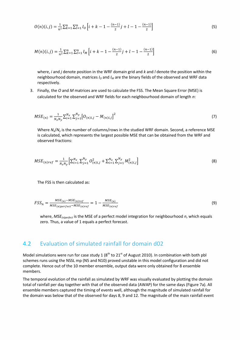
where, i and j denote position in the WRF domain grid and k and l denote the position within the neighbourhood domain, matrices IO and IM are the binary fields of the observed and WRF data respectively.

3. Finally, the O and M matrices are used to calculate the FSS. The Mean Square Error (MSE) is

calculated for the observed and WRF fields for each neighbourhood domain of length n:

(7)

Where Nx/Ny is the number of columns/rows in the studied WRF domain. Second, a reference MSE is calculated, which represents the largest possible MSE that can be obtained from the WRF and observed fractions:

(8)

The FSS is then calculated as:

(9)

where, MSE(n)perfect is the MSE of a perfect model integration for neighbourhood n, which equals zero. Thus, a value of 1 equals a perfect forecast.

4.2 Evaluation of simulated rainfall for domain d02

Model simulations were run for case study 1 (8th to 21st of August 2010). In combination with both pbl schemes runs using the NSSL mp (N5 and N10) proved unstable in this model configuration and did not complete. Hence out of the 10 member ensemble, output data were only obtained for 8 ensemble members.

The temporal evolution of the rainfall as simulated by WRF was visually evaluated by plotting the domain total of rainfall per day together with that of the observed data (AWAP) for the same days (Figure 7a). All ensemble members captured the timing of events well, although the magnitude of simulated rainfall for the domain was below that of the observed for days 8, 9 and 12. The magnitude of the main rainfall event

24 | P a g e

on day 3 to 5 is, however, well captured. The ensemble members show only minor variability in terms of total magnitude rainfall for the simulated domain, with ensemble member N1 (using the combination pbl=MYNN and mp=WDM6) showing marginally smaller bias (Figure 7b).

Simple skill scores were calculated for each day and each completed ensemble member (Figure 8 and Table 7). The bias measure shows that WRF both under and overestimate rainfall occurrence for the simulated time period for all ensemble members but N3, N4 and N8. Overall however, values are close to 1. The accuracy measure (ACC), measuring the fraction of correct simulations relative to all simulations show values in the inter-quartile range of 0.91 and 0.97, with very little variability amongst ensemble members. The false alarm ratio (fraction of false alarms relative to simulated events) and the threat score (hits over all forecasted or observed events) show similar small variability amongst ensemble members, indicating that when using the simple scores there is little to separate the ensemble members in terms of skill.

Figure 7 Temporal evolution of rainfall in domain d02 (case study 1) displayed as grid total rainfall (mm) for WRF members (blue) and AWAP (orange) in panel a, and as bias (difference in grid total rainfall, WRF-AWAP) in panel b

Figure 8 Simple skill scores for domain d02. Upper panel shows ensemble members N1-N4 (using pbl scheme MYNN) and lower panel shows ensemble members N6-N9 (using pbl scheme YSU)

Table 7 For domain d02 and each simple skill score, the median (50th

percentile) and the lower and upper quantile (25

th and 75

th percentile) within brackets

ENSEMBLE MEMBER B ACC FAR TS

N1 1.00 (0.97,1.02) 0.94 (0.91,0.97) 0.03 (0.02,0.04) 0.94 (0.90,0.97)

N2 1.01 (0.98,1.03) 0.93 (0.91,0.96) 0.03 (0.02,0.05) 0.93 (0.91,0.96)

N3 1.02 (1.01,1.05) 0.94 (0.91,0.96) 0.04 (0.03,0.07) 0.93 (0.91,0.96)

N4 1.02 (1.00,1.03) 0.93 (0.91,0.97) 0.04 (0.03,0.05) 0.93 (0.90,0.97)

N6 1.00 (0.98,1.01) 0.94 (0.91,0.97) 0.03 (0.02,0.04) 0.94 (0.90,0.97)

N7 1.00 (0.98,1.01) 0.94 (0.92,0.97) 0.03 (0.02,0.05) 0.93 (0.91,0.97)

N8 1.02 (1.01,1.03) 0.93 (0.92,0.97) 0.04 (0.03,0.06) 0.93 (0.91,0.97)

N9 1.00 (0.99,1.03) 0.94 (0.91,0.97) 0.04 (0.02,0.05) 0.93 (0.91,0.97)

Looking at the FSS, somewhat larger separation can be seen although clearly the ensemble members still show similar skill levels (Figure 9 and Table 8 show results for neighbourhoods of n=1, 3, 5 and 11 grid cells). FSS scores increase, as expected for larger neighbourhoods. Arguably, neighbourhoods corresponding to distances less than 100km would be challenging to obtain a high FSS score as this is the typical spatial scale of convective systems. Nevertheless, this initial evaluation focuses more on relative difference amongst ensemble members than the absolute skill in capturing the observed climate. In this regard, we can see that FSS scores show larger variability between ensemble members of different mp schemes than pbl schemes (Figure 9), where mp scheme Milbrandt (N3 and N8) has the overall lower values and mp scheme WDM6 has overall higher values (N1 and N6). The mp scheme Thompson further

26 | P a g e

show the smallest spread of FSS scores over the 14 day period with somewhat lower values then the Thompson simulations, but generally higher scores than the Milbrandt simulations (Figure 9 and Table 8).

Thus, whilst there appears to be little variability amongst the ensemble members in terms of skill, as assessed using the above metrics, the ensemble member that appeared to perform best (relatively) was N1 using mp scheme WDM6 and pbl scheme MYNN.

Figure 9 FSS for domain d02. Upper panel shows ensemble members N1-N4 (using pbl scheme MYNN) and lower panel shows ensemble members N6-N9 (using pbl scheme YSU). Each group of box plots show the FSS using a neighbourhood length of 1, 3, 5 and 11 grid cells.

Table 8 For domain d02 and for each FSS (neighbourhood length of: 1, 3, 5 and 11 grid cells), the median (50th

percentile) and the lower and upper quantile (25

th and 75

th percentile) within brackets

ENSEMBLE MEMBER FSS, N=1 FSS, N=3 FSS, N=5 FSS, N=11

N1 0.34 (0.18,0.44) 0.46 (0.25,0.62) 0.52 (0.28,0.70) 0.72 (0.40,0.81)

N2 0.30 (0.16,0.34) 0.41 (0.25,0.48) 0.45 (0.29,0.55) 0.60 (0.39,0.68)

N3 0.17 (0.11,0.31) 0.21 (0.16,0.40) 0.23 (0.19,0.47) 0.33 (0.22,0.72)

N4 0.22 (0.07,0.34) 0.30 (0.10,0.50) 0.36 (0.11,0.63) 0.46 (0.26,0.77)

N6 0.30 (0.23,0.42) 0.42 (0.31,0.60) 0.48 (0.38,0.66) 0.66 (0.43,0.76)

N7 0.27 (0.16,0.39) 0.37 (0.22,0.47) 0.41 (0.25,0.53) 0.48 (0.30,0.68)

N8 0.25 (0.10,0.39) 0.33 (0.12,0.58) 0.43 (0.13,0.66) 0.64 (0.14,0.73)

N9 0.23 (0.09,0.36) 0.33 (0.16,0.56) 0.39 (0.23,0.65) 0.49 (0.32,0.79)

4.3 Evaluation of simulated rainfall for domain d03

Model simulations were run for case study 1 (8th to 21st of August 2010). In combination with both pbl schemes, runs using the NSSL mp (N5 and N10) proved unstable in this model configuration and did not complete. Hence out of the 10 member ensemble, output data were only obtained for 8 ensemble members.

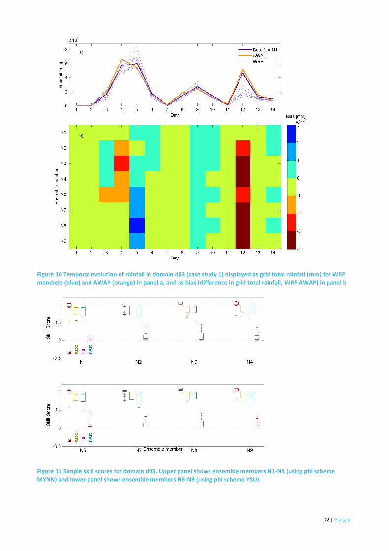
The temporal evolution of the rainfall as simulated by WRF was visually evaluated by plotting the domain total of rainfall per day together with that of the observed data (AWAP) for the same days (Figure 10a). All ensemble members captured the timing of events well up until the last rainfall event of the 14-day period (day 12). For the final event, all but ensemble member N1 underestimated the rainfall falling within domain d03 (Figure 10a and b). The ensemble members showed only minor variability in terms of total magnitude rainfall for the simulated domain, with ensemble member N1 (using the combination pbl=MYNN and mp=WDM6) having the smaller bias (Figure 10b).

Simple skill scores were calculated for each day and each completed ensemble member (Figure 11 and Table 9). The bias measure shows that with the exception of N1, N6 and N7, most ensemble members tend to slightly overestimate rainfall as based on the inter-quantile range (Table 9). The accuracy measure (ACC), measuring the fraction of correct simulations relative to all simulations show that ensemble members are broadly equal in skill with somewhat higher (better) values for simulations using mp schemes Milbrandt and Morrison (N3, N4, N8 and N9), results that largely resonates with results for the threat score (hits over all forecasted or observed events). However, conversely those two schemes together with the Thompson scheme (N2 and N7), perform somewhat worse if considering the false alarm ratio (fraction of false alarms relative to simulated events), where lowest scores are shown for the simulations using the WDM6 mp scheme (N1, N6).

Looking at the FSS, we can clearly see differences in according to mp schemes as well as pbl schemes (Figure 12 and Table 10). Amongst mp schemes, overall larger values (when in combination with a particular pbl scheme) are shown for mp scheme WDM6, and absolutely so when in combination with YSU. Interestingly, mp scheme Milbrandt in combination with pbl scheme MYNN (N3) appears to also show relatively reasonable results, but when in combination with pbl scheme YSU (N8), results are the poorest when compared to other mp schemes. Another mp schemes that appear to perform somewhat better with a particular pbl scheme is Thompson with pbl scheme YSU (N7) (Figure 12).

As in the previous section we note that neighbourhoods corresponding to distances less than 100km would be challenging to obtain a high FSS scores for as this is the typical spatial scale of convective systems. Nevertheless, this initial evaluation focuses more on relative difference amongst ensemble members than the absolute skill in capturing the observed climate.

As for domain d02, whilst there appears to be little variability amongst the ensemble members in terms of skill, as assessed using the above metrics, the ensemble member that appeared to perform best (relatively) was N1 using mp scheme WDM6 and pbl scheme MYNN.

We note that a visual inspection of the rainfall in d03 appears to contain a spurious striation in the rainfall pattern that is not present in the rainfall patterns of d02. It is likely that this pattern arises due to the complex topography or due to disturbances from the lateral boundaries. Further investigation is required to attempt to determine the cause and mitigate using different dynamical settings.

28 | P a g e

Figure 10 Temporal evolution of rainfall in domain d03 (case study 1) displayed as grid total rainfall (mm) for WRF members (blue) and AWAP (orange) in panel a, and as bias (difference in grid total rainfall, WRF-AWAP) in panel b

Figure 11 Simple skill scores for domain d03. Upper panel shows ensemble members N1-N4 (using pbl scheme MYNN) and lower panel shows ensemble members N6-N9 (using pbl scheme YSU).

Table 9 For domain d03 and each simple skill score, the median (50th

percentile) and the lower and upper quantile (25

th and 75

th percentile) within brackets

ENSEMBLE B ACC FAR TS

N1 1.00 (0.96,1.04) 0.93 (0.72,0.97) 0.03 (0.01,0.07) 0.92 (0.69,0.97)

N2 1.01 (1.00,1.03) 0.94 (0.72,0.97) 0.05 (0.02,0.16) 0.93 (0.70,0.97)

N3 1.04 (1.01,1.08) 0.93 (0.78,0.97) 0.07 (0.03,0.20) 0.93 (0.78,0.97)

N4 1.02 (1.00,1.09) 0.92 (0.79,0.98) 0.07 (0.02,0.13) 0.92 (0.79,0.98)

N6 1.00 (0.97,1.02) 0.91 (0.75,0.97) 0.04 (0.01,0.08) 0.91 (0.72,0.97)

N7 1.01 (0.99,1.03) 0.93 (0.78,0.97) 0.05 (0.02,0.13) 0.93 (0.70,0.97)

N8 1.04 (1.01,1.09) 0.92 (0.79,0.97) 0.07 (0.03,0.20) 0.92 (0.79,0.97)

N9 1.03 (1.00,1.08) 0.92 (0.79,0.97) 0.07 (0.03,0.15) 0.92 (0.79,0.97)

Figure 12 FSS for domain d03. Upper panel shows ensemble members N1-N4 (using pbl scheme MYNN) and lower panel shows ensemble members N6-N9 (using pbl scheme YSU). Each group of box plots show the FSS using a neighbourhood length of 1, 3, 5 and 11 grid cells.

30 | P a g e

Table 10 For domain d03 and for each FSS (neighbourhood length of: 1, 3, 5 and 11 grid cells), the median (50th

percentile) and the lower and upper quantile (25

th and 75

th percentile) within brackets

ENSEMBLE MEMBER FSS, N=1 FSS, N=3 FSS, N=5 FSS, N=11

N1 0.16 (0.00,0.23) 0.16 (0.00,0.28) 0.16 (0.00,0.31) 0.17 (0.00,0.40)

N2 0.09 (0.00,0.17) 0.11 (0.00,0.21) 0.14 (0.00,0.25) 0.21 (0.00,0.28)

N3 0.06 (0.00,0.28) 0.08 (0.00,0.33) 0.10 (0.00,0.36) 0.17 (0.00,0.35)

N4 0.07 (0.00,0.22) 0.09 (0.00,0.22) 0.10 (0.00,0.24) 0.16 (0.00,0.30)

N6 0.12 (0.00,0.27) 0.13 (0.00,0.34) 0.14 (0.00,0.39) 0.15 (0.00,0.47)

N7 0.09 (0.00,0.25) 0.12 (0.00,0.30) 0.14 (0.00,0.34) 0.20 (0.00,0.40)

N8 0.06 (0.00,0.11) 0.09 (0.00,0.15) 0.10 (0.00,0.18) 0.13 (0.00,0.31)

N9 0.03 (0.00,0.18) 0.05 (0.00,0.24) 0.06 (0.00,0.28) 0.13 (0.00,0.40)

5 Summary

This technical report records the decisions underpinning the experimental setup of WRF modelling system for Project 6 of VicCI and provides a rationale for the temporal and spatial dimensions of the case studies used to assess the selected WRF configuration.

A 10-member ensemble was identified for testing, focusing in particular on more complex microphysics schemes in combination with two different pbl schemes, the MYNN and YSU.

Further, three case study periods were identified focusing on catchments to the west and south of the Great Dividing Range. The three case study periods were identified in a two stage process involving consultation with stakeholders at DEPI and BoM and a visual assessment of rainfall events and synoptic circulation during the identified period of interest. In total three study periods of 2 weeks each were selected: 8th to 21st of August 2010, 6th to 19th of October 2010 and 31st of January 2011 to 13th of February 2011.

A three nested configuration (50 km/10 km/2 km) of WRF was applied to the first case study period. During this run only 8 of 10 ensemble members proved stable under the chosen configuration; runs using the mp scheme NSSL became unstable and terminated.

A first look at results from the first case study suggests that simulation of rainfall in the 10km domain had good skill as judged by a number of skill scores. However, model performance in the innermost domain (2km) proved worse, and a visual assessment of rainfall patterns indicate spurious striation in the rainfall pattern, which may be corrected by different choices of dampening or movement of the lateral boundaries away from complex topography.

Using a set of skill metrics and visual evaluation, rainfall magnitudes and patterns were assessed for domain d02 (10km) and d03 (2km) against observed data set AWAP. For both domains, a somewhat better performance (as judged by the used metrics) was gained by simulations using mp scheme WDM6 in combination with pbl scheme MYNN. To separate skill amongst WRF configurations, further evaluation is required, e.g. looking at other variables and assessing why rainfall patterns differ amongst the ensemble members.

32 | P a g e

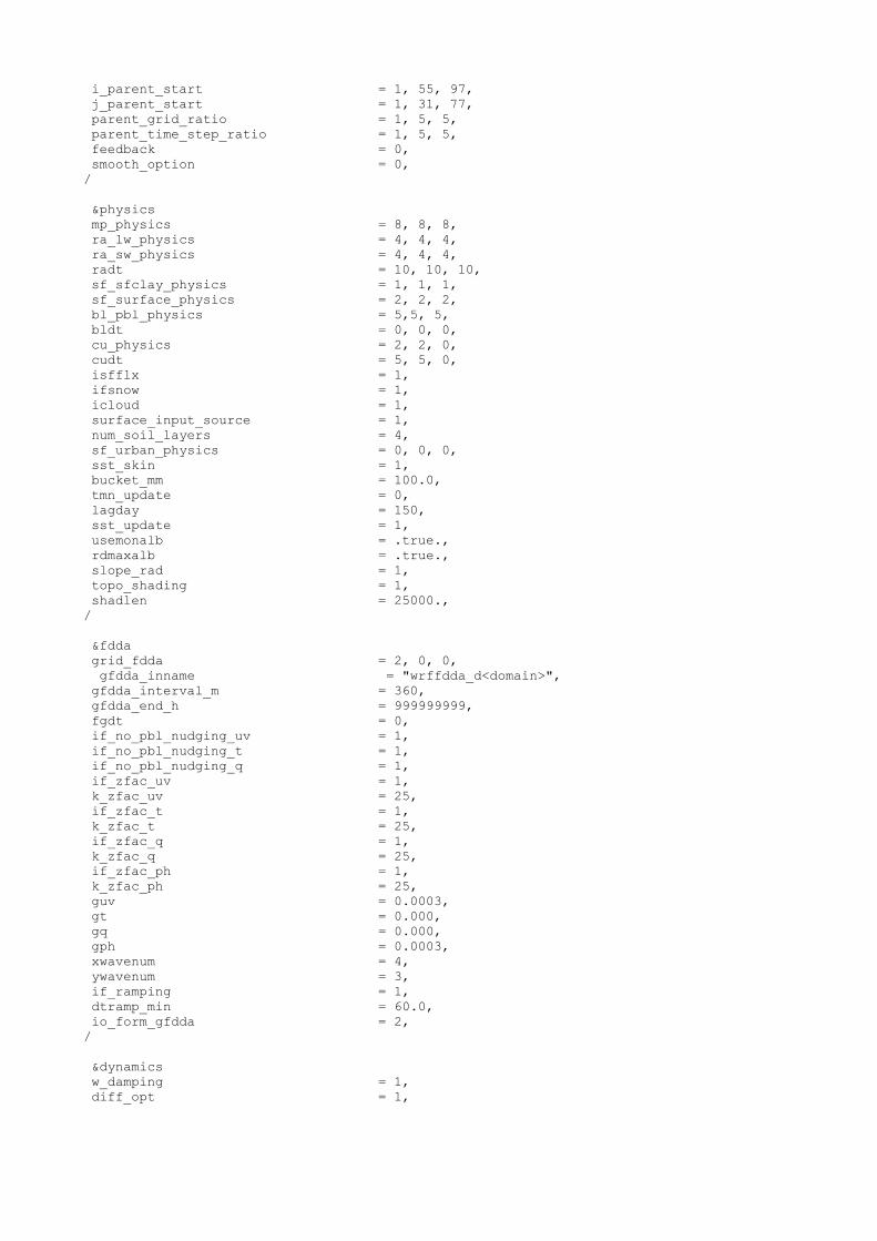
Appendix A Parameter file ‘namelist.input’

Below follows an example of a parameter file (here for Study region 1, ensemble member N3):

&time_control

run_days = 0,

run_hours = 00,

run_minutes = 0,

run_seconds = 0,

start_year = 2010, 2010, 2010,

start_month = 08, 08, 08,

start_day = 06, 06, 06,

start_hour = 00, 00, 00,

start_minute = 00, 00, 00,

start_second = 00, 00, 00,

end_year = 2010, 2010, 2010,

end_month = 08, 08, 08,

end_day = 22, 22, 22,

end_hour = 00, 00, 00,

end_minute = 00, 00, 00,

end_second = 00, 00, 00,

interval_seconds = 21600

input_from_file = .true.,.true.,.true.,

history_interval = 180, 60, 60,

frames_per_outfile = 8, 24, 24,

restart = .false.,

restart_interval = 21600,

io_form_history = 2

io_form_restart = 2

io_form_input = 2

io_form_boundary = 2

debug_level = 0

auxinput4_inname = "wrflowinp_d<domain>"

io_form_auxinput4 = 2

auxinput4_interval = 360, 360, 360,

/

&Options for adaptive time step

use_adaptive_time_step = .true.,

step_to_output_time = .true.,

adjust_output_times = .true.,

target_cfl = 1.2, 1.2, 1.2,

target_hcfl = 0.84, 0.84, 0.84,

max_step_increase_pct = 5, 51, 51,

starting_time_step = -1, -1, -1,

max_time_step = 360, 120, 40,

min_time_step = 90, 30, 10,

adaptation_domain = 1,

/

&domains

time_step = 300

time_step_fract_num = 0,

time_step_fract_den = 1,

max_dom = 3,

e_we = 143, 236, 296,

e_sn = 125, 181, 236,

e_vert = 40, 40, 40,

p_top_requested = 5000,

num_metgrid_levels = 38,

num_metgrid_soil_levels = 4,

dx = 50000, 10000, 2000,

dy = 50000, 10000, 2000,

grid_id = 1, 2, 3,

parent_id = 0, 1, 2,

i_parent_start = 1, 55, 97,

j_parent_start = 1, 31, 77,

parent_grid_ratio = 1, 5, 5,

parent_time_step_ratio = 1, 5, 5,

feedback = 0,

smooth_option = 0,

/

&physics

mp_physics = 8, 8, 8,

ra_lw_physics = 4, 4, 4,

ra_sw_physics = 4, 4, 4,

radt = 10, 10, 10,

sf_sfclay_physics = 1, 1, 1,

sf_surface_physics = 2, 2, 2,

bl_pbl_physics = 5,5, 5,

bldt = 0, 0, 0,

cu_physics = 2, 2, 0,

cudt = 5, 5, 0,

isfflx = 1,

ifsnow = 1,

icloud = 1,

surface_input_source = 1,

num_soil_layers = 4,

sf_urban_physics = 0, 0, 0,

sst_skin = 1,

bucket_mm = 100.0,

tmn_update = 0,

lagday = 150,

sst_update = 1,

usemonalb = .true.,

rdmaxalb = .true.,

slope_rad = 1,

topo_shading = 1,

shadlen = 25000.,

/

&fdda

grid_fdda = 2, 0, 0,

gfdda_inname = "wrffdda_d<domain>",

gfdda_interval_m = 360,

gfdda_end_h = 999999999,

fgdt = 0,

if_no_pbl_nudging_uv = 1,

if_no_pbl_nudging_t = 1,

if_no_pbl_nudging_q = 1,

if_zfac_uv = 1,

k_zfac_uv = 25,

if_zfac_t = 1,

k_zfac_t = 25,

if_zfac_q = 1,

k_zfac_q = 25,

if_zfac_ph = 1,

k_zfac_ph = 25,

guv = 0.0003,

gt = 0.000,

gq = 0.000,

gph = 0.0003,

xwavenum = 4,

ywavenum = 3,

if_ramping = 1,

dtramp_min = 60.0,

io_form_gfdda = 2,

/

&dynamics

w_damping = 1,

diff_opt = 1,

34 | P a g e

km_opt = 4,

diff_6th_opt = 2, 2, 2,

diff_6th_factor = 0.12, 0.12, 0.12,

base_temp = 290.

damp_opt = 3,

zdamp = 5000., 5000., 5000.,

dampcoef = 0.2, 0.2, 0.2,

khdif = 0, 0, 0,

kvdif = 0, 0, 0,

non_hydrostatic = .true.,.true.,.true.,

moist_adv_opt = 1, 1, 1,

scalar_adv_opt = 1, 1, 1,

gwd_opt = 1,

epssm = 0.2, 0.2, 0.2,

/

&bdy_control

spec_bdy_width = 10,

spec_zone = 1,

relax_zone = 9,

specified = .true.,.false.,.false.,

spec_exp = 0.33,

nested = .false.,.true.,.true.,

/

&grib2

/

&namelist_quilt

nio_tasks_per_group = 0,

nio_groups = 1,

/

Appendix B Vtable for WRF pre-processor: Vtable.ERA-interim.pl

GRIB | Level| Level| Level| metgrid | metgrid | metgrid |

Code | Code | 1 | 2 | Name | Units | Description |

-----+------+------+------+----------+----------+------------------------------------------+

129 | 100 | * | | GEOPT | m2 s-2 | |

| 100 | * | | HGT | m | Height |

130 | 100 | * | | TT | K | Temperature |

131 | 100 | * | | UU | m s-1 | U |

132 | 100 | * | | VV | m s-1 | V |

157 | 100 | * | | RH | % | Relative Humidity |

165 | 1 | 0 | | UU | m s-1 | U | At 10 m

166 | 1 | 0 | | VV | m s-1 | V | At 10 m

167 | 1 | 0 | | TT | K | Temperature | At 2 m

168 | 1 | 0 | | DEWPT | K | | At 2 m

| 1 | 0 | | RH | % | Relative Humidity | At 2 m

172 | 1 | 0 | | LANDSEA | 0/1 Flag | Land/Sea flag |

129 | 1 | 0 | | SOILGEO | m2 s-2 | |

| 1 | 0 | | SOILHGT | m | Terrain field of source analysis |

134 | 1 | 0 | | PSFC | Pa | Surface Pressure |

151 | 1 | 0 | | PMSL | Pa | Sea-level Pressure |

235 | 1 | 0 | | SKINTEMP | K | Sea-Surface Temperature |

31 | 1 | 0 | | SEAICE | fraction | Sea-Ice Fraction |

34 | 1 | 0 | | SST | K | Sea-Surface Temperature |

33 | 1 | 0 | | SNOW_DEN | kg m-3 | |

141 | 1 | 0 | | SNOW_EC | m | |

| 1 | 0 | | SNOW | kg m-2 |Water Equivalent of Accumulated Snow Depth|

| 1 | 0 | | SNOWH | m | Physical Snow Depth |

139 | 112 | 0 | 7 | ST000007 | K | T of 0-7 cm ground layer |

170 | 112 | 7 | 28 | ST007028 | K | T of 7-28 cm ground layer |

183 | 112 | 28 | 100 | ST028100 | K | T of 28-100 cm ground layer |

236 | 112 | 100 | 255 | ST100255 | K | T of 100-255 cm ground layer |

39 | 112 | 0 | 7 | SM000007 | m3 m-3 | Soil moisture of 0-7 cm ground layer |

40 | 112 | 7 | 28 | SM007028 | m3 m-3 | Soil moisture of 7-28 cm ground layer |

41 | 112 | 28 | 100 | SM028100 | m3 m-3 | Soil moisture of 28-100 cm ground layer |

42 | 112 | 100 | 255 | SM100255 | m3 m-3 | Soil moisture of 100-255 cm ground layer |

-----+------+------+------+----------+----------+------------------------------------------+

#

# For use with ERA-interim pressure-level output.

#

# Grib codes are from Table 128

# http://www.ecmwf.int/services/archive/d/parameters/order=grib_parameter/table=128/

#

# snow depth is converted to the proper units in rrpr.F

#

# For ERA-interim data at NCAR, use the pl (sc and uv) and sfc sc files.

36 | P a g e

References

COMRIE, N. 2011. Review of the 2010–11 Flood Warnings & Response Melbourne, Victoria, Australia. CONIGLIO, M. C., CORREIA, J., JR., MARSH, P. T. & KONG, F. 2013. Verification of Convection-Allowing WRF Model Forecasts of the

Planetary Boundary Layer Using Sounding Observations. Weather and Forecasting, 28, 842-862. DEE, D. P., UPPALA, S. M., SIMMONS, A. J., BERRISFORD, P., POLI, P., KOBAYASHI, S., ANDRAE, U., BALMASEDA, M. A., BALSAMO, G.,

BAUER, P., BECHTOLD, P., BELJAARS, A. C. M., VAN DE BERG, L., BIDLOT, J., BORMANN, N., DELSOL, C., DRAGANI, R., FUENTES, M., GEER, A. J., HAIMBERGER, L., HEALY, S. B., HERSBACH, H., HOLM, E. V., ISAKSEN, L., KALLBERG, P., KOEHLER, M., MATRICARDI, M., MCNALLY, A. P., MONGE-SANZ, B. M., MORCRETTE, J. J., PARK, B. K., PEUBEY, C., DE ROSNAY, P., TAVOLATO, C., THEPAUT, J. N. & VITART, F. 2011. The ERA-Interim reanalysis: configuration and performance of the data assimilation system. Quarterly Journal of the Royal Meteorological Society, 137, 553-597.

DUDHIA, J. 1989. NUMERICAL STUDY OF CONVECTION OBSERVED DURING THE WINTER MONSOON EXPERIMENT USING A MESOSCALE TWO-DIMENSIONAL MODEL. Journal of the Atmospheric Sciences, 46, 3077-3107.

EVANS, J. P., EKSTROEM, M. & JI, F. 2012. Evaluating the performance of a WRF physics ensemble over South-East Australia. Climate Dynamics, 39, 1241-1258.

HONG, S.-Y., NOH, Y. & DUDHIA, J. 2006. A new vertical diffusion package with an explicit treatment of entrainment processes. Monthly Weather Review, 134, 2318-2341.

HONG, S. Y., DUDHIA, J. & CHEN, S. H. 2004. A revised approach to ice microphysical processes for the bulk parameterization of clouds and precipitation. Monthly Weather Review, 132, 103-120.

HONG, S. Y. & PAN, H. L. 1996. Nonlocal boundary layer vertical diffusion in a Medium-Range Forecast Model. Monthly Weather Review, 124, 2322-2339.

IACONO, M. J., DELAMERE, J. S., MLAWER, E. J., SHEPHARD, M. W., CLOUGH, S. A. & COLLINS, W. D. 2008. Radiative forcing by long-lived greenhouse gases: Calculations with the AER radiative transfer models. Journal of Geophysical Research-Atmospheres, 113.

JANJIC, Z. I. 1994. THE STEP-MOUNTAIN ETA COORDINATE MODEL - FURTHER DEVELOPMENTS OF THE CONVECTION, VISCOUS SUBLAYER, AND TURBULENCE CLOSURE SCHEMES. Monthly Weather Review, 122, 927-945.

JANJIC, Z. I. 2000. Comments on "Development and evaluation of a convection scheme for use in climate models". Journal of the Atmospheric Sciences, 57, 3686-3686.

JONES, D. A., WANG, W. & FAWCETT, R. 2009. High-quality spatial climate data-sets for Australia. Australian Meteorological and Oceanographic Journal, 58, 233-248.

LIM, K.-S. S. & HONG, S.-Y. 2010. Development of an Effective Double-Moment Cloud Microphysics Scheme with Prognostic Cloud Condensation Nuclei (CCN) for Weather and Climate Models. Monthly Weather Review, 138, 1587-1612.

LIU, P., TSIMPIDI, A. P., HU, Y., STONE, B., RUSSELL, A. G. & NENES, A. 2012. Differences between downscaling with spectral and grid nudging using WRF. Atmospheric Chemistry and Physics, 12.

MANSELL, E. R., ZIEGLER, C. L. & BRUNING, E. C. 2010. Simulated Electrification of a Small Thunderstorm with Two-Moment Bulk Microphysics. Journal of the Atmospheric Sciences, 67, 171-194.

MILBRANDT, J. A. & YAU, M. K. 2005. A multimoment bulk microphysics parameterization. Part II: A proposed three-moment closure and scheme description. Journal of the Atmospheric Sciences, 62, 3065-3081.

MITTERMAIER, M., ROBERTS, N. & THOMPSON, S. A. 2013. A long-term assessment of precipitation forecast skill using the Fractions Skill Score. Meteorological Applications, 20, 176-186.

MLAWER, E. J., TAUBMAN, S. J., BROWN, P. D., IACONO, M. J. & CLOUGH, S. A. 1997. Radiative transfer for inhomogeneous atmospheres: RRTM, a validated correlated-k model for the longwave. Journal of Geophysical Research-Atmospheres, 102, 16663-16682.

MOLINARI, J. & DUDEK, M. 1986. IMPLICIT VERSUS EXPLICIT CONVECTIVE HEATING IN NUMERICAL WEATHER PREDICTION MODELS. Monthly Weather Review, 114, 1822-1831.

NAKANISHI, M. & NIINO, H. 2006. An improved mellor-yamada level-3 model: Its numerical stability and application to a regional prediction of advection fog. Boundary-Layer Meteorology, 119, 397-407.

NCAR 2013. ARW Version 3 Modelling System User's Guide. Mesoscale & Microscale Meteorology Division, National Centre for Atmospheric Research

RAISANEN, P. 1998. Effective longwave cloud fraction and maximum-random overlap of clouds: A problem and a solution. Monthly Weather Review, 126, 3336-3340.

ROBERTS, N. 2008. Assessing the spatial and temporal variation in the skill of precipitation forecasts from an NWP model. Meteorological Applications, 15, 163-169.

ROBERTS, N. M. & LEAN, H. W. 2008. Scale-selective verification of rainfall accumulations from high-resolution forecasts of convective events. Monthly Weather Review, 136, 78-97.

SKAMAROCK, W. C. & KLEMP, J. B. 2008. A time-split nonhydrostatic atmospheric model for weather research and forecasting applications. Journal of Computational Physics, 227, 3465-3485.

THOMPSON, G., FIELD, P. R., RASMUSSEN, R. M. & HALL, W. D. 2008. Explicit Forecasts of Winter Precipitation Using an Improved Bulk Microphysics Scheme. Part II: Implementation of a New Snow Parameterization. Monthly Weather Review, 136, 5095-5115.

WILKS, D. 2006. Statistical methods in the atmospheric sciences, US, Elsevier.

38 | P a g e

CONTACT US

t 1300 363 400 +61 3 9545 2176 e enquiries@csiro.au w www.csiro.au

YOUR CSIRO

Australia is founding its future on science and innovation. Its national science agency, CSIRO, is a powerhouse of ideas, technologies and skills for building prosperity, growth, health and sustainability. It serves governments, industries, business and communities across the nation.

FOR FURTHER INFORMATION

CLW/Unit Name Marie Ekström t +61 2 6246 5986 e marie.ekstrom@csiro.au w www.csiro.au