Tessellation and Lyubich-Minsky laminations associated withquadratic maps I: Pinching semiconjugacies

Tomoki KawahiraGraduate School of Mathematics, Nagoya University

May 13, 2007

Abstract

We introduce tessellation of the filled Julia sets for hyperbolic and parabolicquadratic maps. Then the dynamics inside their Julia sets are organized by tileswhich work like external rays outside. We also construct continuous families of pinch-ing semiconjugacies associated with hyperblic-to-parabolic degenerations without us-ing quasiconformal deformation. Instead we use tessellation and investigation on thehyperbolic-to-parabolic degeneration of linearizing coordinates inside the Julia set.

1 Introduction

After the works by Douady and Hubbard, dynamics of quadratic map f = fc : z �→z2 + c with an attracting or parabolic cycle has been investigated in detail, because suchparameters c of fc are contained in the Mandelbrot set and they are very importantelements that determine the topology of the Mandelbrot set. (See [DH] or [Mi2].)

The aim of this paper is to provide a new method to describe combinatorial changesof dynamics when the parameter c moves from one hyperbolic component to another viaa “parabolic parameter” (i.e., c of fc with a parabolic cycle).

For example, the simplest case is the motion in the Mandelbrot set along a path joiningc = 0 and the center cp/q of the p/q-satellite component of the main cardioid via the rootof p/q-limb. In particular, we join them by the two segments characterized as follows:

(s1) c of fc which has a fixed point of multiplier re2πip/q with 0 < r ≤ 1; and

(s2) c of fc which has a q-periodic cycle of multiplier 1 ≥ r > 0.

Note that we avoid the hyperbolic centers (i.e., c of fc with superattracting cycle) becausewe regard them as non-generic special cases far away from parabolic bifurcations.

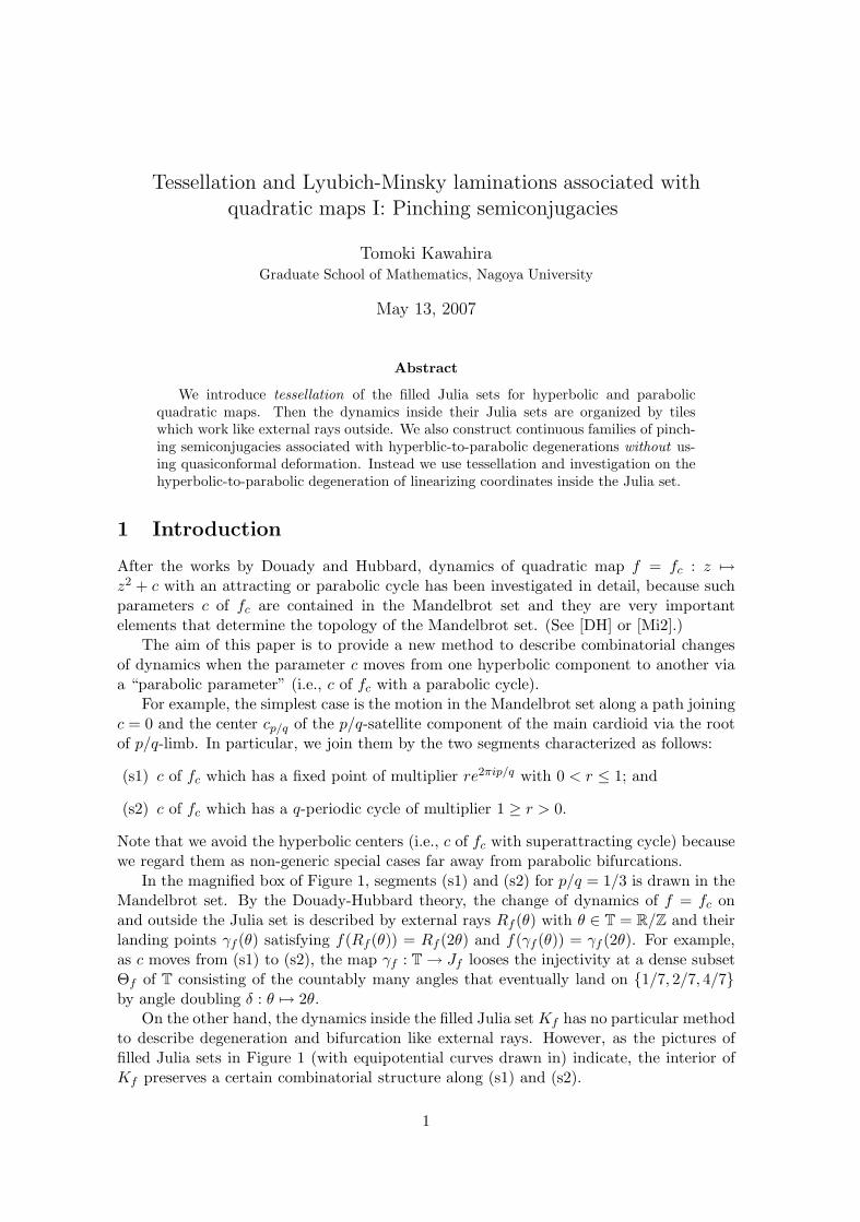
In the magnified box of Figure 1, segments (s1) and (s2) for p/q = 1/3 is drawn in theMandelbrot set. By the Douady-Hubbard theory, the change of dynamics of f = fc onand outside the Julia set is described by external rays Rf (θ) with θ ∈ T = R/Z and theirlanding points γf (θ) satisfying f(Rf (θ)) = Rf (2θ) and f(γf (θ)) = γf (2θ). For example,as c moves from (s1) to (s2), the map γf : T → Jf looses the injectivity at a dense subsetΘf of T consisting of the countably many angles that eventually land on {1/7, 2/7, 4/7}by angle doubling δ : θ �→ 2θ.

On the other hand, the dynamics inside the filled Julia setKf has no particular methodto describe degeneration and bifurcation like external rays. However, as the pictures offilled Julia sets in Figure 1 (with equipotential curves drawn in) indicate, the interior ofKf preserves a certain combinatorial structure along (s1) and (s2).

1

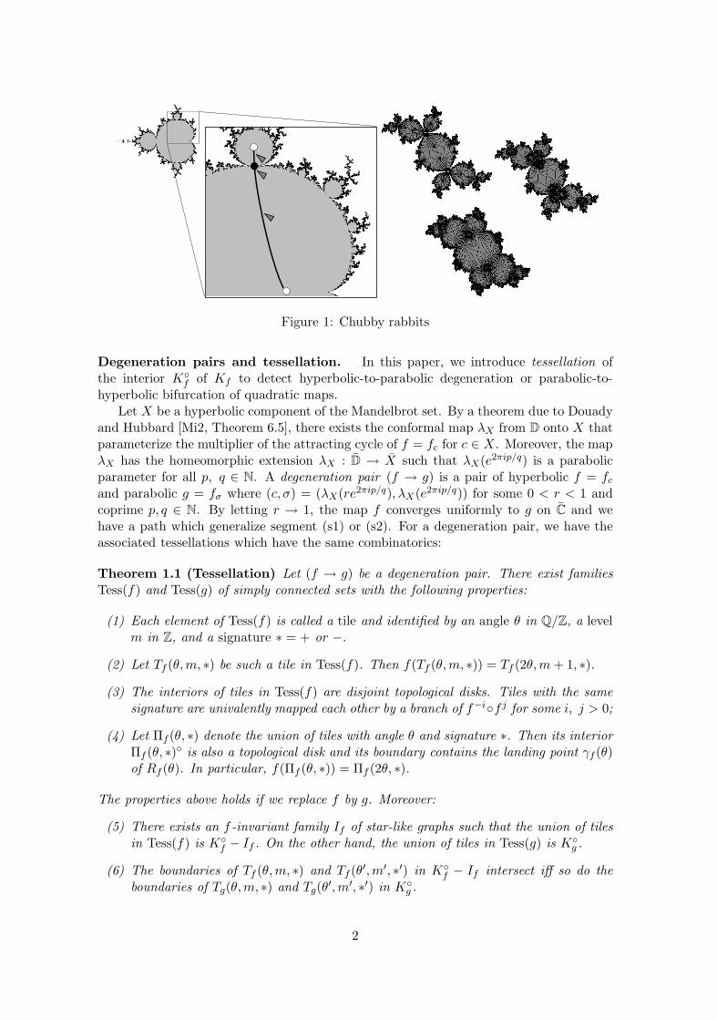
Figure 1: Chubby rabbits

Degeneration pairs and tessellation. In this paper, we introduce tessellation ofthe interior K◦

f of Kf to detect hyperbolic-to-parabolic degeneration or parabolic-to-hyperbolic bifurcation of quadratic maps.

Let X be a hyperbolic component of the Mandelbrot set. By a theorem due to Douadyand Hubbard [Mi2, Theorem 6.5], there exists the conformal map λX from D onto X thatparameterize the multiplier of the attracting cycle of f = fc for c ∈ X. Moreover, the mapλX has the homeomorphic extension λX : D → X such that λX(e2πip/q) is a parabolicparameter for all p, q ∈ N. A degeneration pair (f → g) is a pair of hyperbolic f = fc

and parabolic g = fσ where (c, σ) = (λX(re2πip/q), λX(e2πip/q)) for some 0 < r < 1 andcoprime p, q ∈ N. By letting r → 1, the map f converges uniformly to g on C and wehave a path which generalize segment (s1) or (s2). For a degeneration pair, we have theassociated tessellations which have the same combinatorics:

Theorem 1.1 (Tessellation) Let (f → g) be a degeneration pair. There exist familiesTess(f) and Tess(g) of simply connected sets with the following properties:

(1) Each element of Tess(f) is called a tile and identified by an angle θ in Q/Z, a levelm in Z, and a signature ∗ = + or −.

(2) Let Tf (θ,m, ∗) be such a tile in Tess(f). Then f(Tf (θ,m, ∗)) = Tf (2θ,m+ 1, ∗).(3) The interiors of tiles in Tess(f) are disjoint topological disks. Tiles with the same

signature are univalently mapped each other by a branch of f−i◦f j for some i, j > 0;

(4) Let Πf (θ, ∗) denote the union of tiles with angle θ and signature ∗. Then its interiorΠf (θ, ∗)◦ is also a topological disk and its boundary contains the landing point γf (θ)of Rf (θ). In particular, f(Πf (θ, ∗)) = Πf (2θ, ∗).

The properties above holds if we replace f by g. Moreover:

(5) There exists an f -invariant family If of star-like graphs such that the union of tilesin Tess(f) is K◦

f − If . On the other hand, the union of tiles in Tess(g) is K◦g .

(6) The boundaries of Tf (θ,m, ∗) and Tf (θ′,m′, ∗′) in K◦f − If intersect iff so do the

boundaries of Tg(θ,m, ∗) and Tg(θ′,m′, ∗′) in K◦g .

2

1/7

167/819215/819167/819167/819

215/819215/819

167/819

164/819

164/819

164/819164/819

1/7

0

00

1/3

1/3

2/3 2/3

1/3

22/6322/63

25/63

25/63

37/63 3/7

3/7

4/7

2/7

2/7 4/15

4/15

1/5

1/5

4/7

1/72/7

4/7

Figure 2: Samples of tessellation. For the two figures at the upper left, parameters aretaken from period 12 and 4 hyperbolic components of the Mandelbrot set as indicated inthe figure of a small Mandelbrot set.

3

Here angles of tiles must be the angles of external rays which eventually land on theparabolic cycle of g. (For example, if (f → g) are on (s1) or (s2) in Figure 1, the set ofangles of tiles coincides with Θf .) See Sections 2 and 3 for construction of tessellation andFigure 2 for examples. One can find that the combinatorics of tessellations are preservedalong (s1) and (s2). (This is justified in Section 4 more generally.) Since fc ∈ X−{λX(0)}is structurally stable, we have the tessellation of Kfc with the same properties of Tess(f).

Pinching semiconjugacy. As an application of tessellation, we show that there existsa pinching semiconjugacy from f to g for the degeneration pair (f → g). In Sections 4and 5 we will establish:

Theorem 1.2 (Pinching semiconjugacy) Let (f → g) be a degeneration pair. Thereexists a semiconjugacy h : C → C from f to g such that:

(1) h only pinches If to the grand orbit of the parabolic cycle of g.

(2) h sends all possible Tf (θ,m, ∗) to Tg(θ,m, ∗), Rf (θ) to Rg(θ), and γf (θ) to γg(θ).

(3) h tends to the identity as f tends to g.

One may easily imagine the situation by seeing the figures of tessellation. As a corollary,we have convergence of the tiles when f of (f → g) tends to g (Corollary 5.2).

We first prove the existence of h with properties (1) and (2) in Section 4 (Theorem4.1) by using combinatorial properties of tessellation. Property (3) is proved in Section 5(Theorem 5.1) by means of the continuity results about the extended Bottcher coordinates(Theorem 5.4) on and outside the Julia sets and the linearizing coordinates (i.e., the Konigsand Fatou coordinates) inside the Julia sets associated with (f → g) (Theorem 5.5).

In Appendix, we will give some useful results on perturbation of parabolics used forthe proof.

Notes.

1. For any fc ∈ X −{λX(0)}, we have a semiconjugacy hc which has similar propertiesto (1) and (2) by structural stability. By results of Cui ([Cu]), Haıssinsky andTan Lei([Ha2], [HT]), it is already known that such a semiconjugacy exists. Theirmethod is based on the quasiconformal deformation theory and works even for somegeometrically infinite rational maps. On the other hand, our method is faithful tothe quadratic dynamics and the semiconjugacy is constructed in a more explicit waywithout using quasiconformal deformation. It is possible to extend our results tosome class of higher degree polynomials or rational maps but it is out of our scope.

2. This paper is the first part of works on Lyubich-Minsky laminations. In [LM], theyintroduced the hyperbolic 3-laminations associated with rational maps as an ana-logue of the hyperbolic 3-manifolds associated with Kleinian groups. In the secondpart of this paper [Ka3], we will investigate combinatorial and topological changeof 3-laminations associated with hyperbolic-to-parabolic degeneration of quadraticmaps by means of tessellation and pinching semiconjugacies.

3. The most recent version of this paper and author’s other articles are available at:http://www.math.nagoya-u.ac.jp/~kawahira

Acknowledgments. I would like to thank M. Lyubich for giving opportunities to visitSUNY at Stony Brook, University of Toronto, and the Fields Institute where a part of this

4

work was being prepared. This research is partially supported by JSPS Research Fellow-ships for Young Scientists, JSPS Grant-in-Aid for Young Scientists, Nagoya University,the Circle for the Promotion of Science and Engineering, and Inamori Foundation.

2 Degeneration pair and degenerating arc system

Segments (s1) and (s2) in the previous section are considered as hyperbolic-to-parabolicdegeneration processes of two distinct directions. Degeneration pairs generalize all ofsuch processes in the quadratic family. The aim of this section is to give a dichotomousclassification of the degeneration pairs {(f → g)} and to define invariant families of star-like graphs (degenerating arc systems) for each f of (f → g).

Classification of degeneration pairs. We first fix some notation used throughoutthis paper. Let p and q be relatively prime positive integers, and set ω := exp(2πip/q).(We allow the case of p = q = 1.) Take an r from the interval (0, 1) and set λ := rω. As inthe previous section, we take a hyperbolic component X of the Mandelbrot set. Then wehave a degeneration pair (f → g) that is a pair of hyperbolic f = fc and parabolic g = fσ

where (c, σ) = (λX(re2πip/q), λX(e2πip/q)).For the degeneration pair (f → g), let Of := {α1, . . . , αl} be the attracting cycle

of f with multiplier λ = rω and f(αj) = αj+1 (taking subscripts modulo l). Similarly,let Og := {β1, . . . , βl′} be the parabolic cycle of g with g(βj′) = βj′+1 (taking subscriptsmodulo l′). Let ω′ = e2πip′/q′ denote the multiplier of Og with relatively prime positiveintegers p′ and q′. (Then Og is a parabolic cycle with q′ repelling petals.)

Our fundamental classification is described by the following proposition:

Proposition 2.1 Any degeneration pair (f → g) satisfies either

Case (a): q = q′ and l = l′; or

Case (b): q = 1 < q′ and l = l′q′.

For both cases, we have lq = l′q′.

The proof is given by summing up results in sections 2, 4 and 6 of [Mi2]. For example,a degeneration pair (f → g) on segment (s1) (resp. (s2)) with q > 1 is a Case (a) (resp.Case(b)) above. Degeneration pairs (fc → fσ) with σ = 1/4 or σ = −7/4 satisfy q = q′ = 1and thus Case (a).

Note on terminology. According to [Mi2], a parabolic g with q′ = 1 is called primitive.The parabolic g = fσ with σ = 1/4 is also called trivial. For these g’s any degeneration pair(f → g) is automatically Case (a) by the proposition above. When we define tessellationfor non-trivial primitive (f → g), a little extra care will be required.

Perturbation of Og and degenerating arcs. For a degeneration pair (f → g) withr ≈ 1, the parabolic cycle Og is approximated by an attracting or repelling cycle O′

f withthe same period l′ and multiplier λ′ ≈ e2πip′/q′ . Let α′

1 be the point in O′f with α′

1 → β1

as r → 1. (cf. [Mi2, §4])In Case (a), the cycle O′

f is attracting (thus O′f = Of ) and there are q′ symmetrically

arrayed repelling periodic points around α1 = α′1. Then we will show that there exits

an f l′-invariant star-like graph I(α′1) that joins α′

1 and the repelling periodic points by q′

arcs. In Case (b), the cycle O′f is repelling and there are q′ = l/l′ symmetrically arrayed

5

attracting periodic points around α′1. Then we will show that there exits an f l′-invariant

star-like graph I(α′1) that joins α′

1 and the attracting periodic points by q′ arcs.In both cases, we define degenerating arc system If by

If :=⋃n≥0

f−n(I(α′1)).

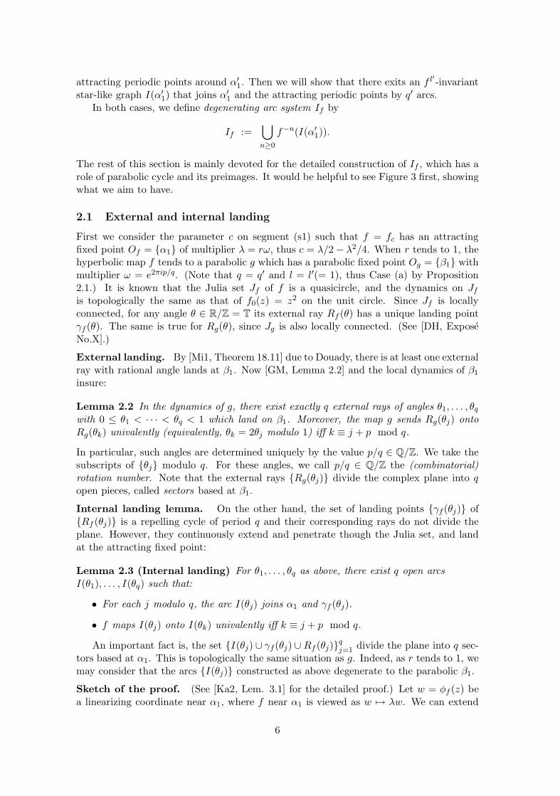
The rest of this section is mainly devoted for the detailed construction of If , which has arole of parabolic cycle and its preimages. It would be helpful to see Figure 3 first, showingwhat we aim to have.

2.1 External and internal landing

First we consider the parameter c on segment (s1) such that f = fc has an attractingfixed point Of = {α1} of multiplier λ = rω, thus c = λ/2 − λ2/4. When r tends to 1, thehyperbolic map f tends to a parabolic g which has a parabolic fixed point Og = {β1} withmultiplier ω = e2πip/q. (Note that q = q′ and l = l′(= 1), thus Case (a) by Proposition2.1.) It is known that the Julia set Jf of f is a quasicircle, and the dynamics on Jf

is topologically the same as that of f0(z) = z2 on the unit circle. Since Jf is locallyconnected, for any angle θ ∈ R/Z = T its external ray Rf (θ) has a unique landing pointγf (θ). The same is true for Rg(θ), since Jg is also locally connected. (See [DH, ExposeNo.X].)

External landing. By [Mi1, Theorem 18.11] due to Douady, there is at least one externalray with rational angle lands at β1. Now [GM, Lemma 2.2] and the local dynamics of β1

insure:

Lemma 2.2 In the dynamics of g, there exist exactly q external rays of angles θ1, . . . , θq

with 0 ≤ θ1 < · · · < θq < 1 which land on β1. Moreover, the map g sends Rg(θj) ontoRg(θk) univalently (equivalently, θk = 2θj modulo 1) iff k ≡ j + p mod q.

In particular, such angles are determined uniquely by the value p/q ∈ Q/Z. We take thesubscripts of {θj} modulo q. For these angles, we call p/q ∈ Q/Z the (combinatorial)rotation number. Note that the external rays {Rg(θj)} divide the complex plane into qopen pieces, called sectors based at β1.

Internal landing lemma. On the other hand, the set of landing points {γf (θj)} of{Rf (θj)} is a repelling cycle of period q and their corresponding rays do not divide theplane. However, they continuously extend and penetrate though the Julia set, and landat the attracting fixed point:

Lemma 2.3 (Internal landing) For θ1, . . . , θq as above, there exist q open arcsI(θ1), . . . , I(θq) such that:

• For each j modulo q, the arc I(θj) joins α1 and γf (θj).

• f maps I(θj) onto I(θk) univalently iff k ≡ j + p mod q.

An important fact is, the set {I(θj) ∪ γf (θj) ∪Rf (θj)}qj=1 divide the plane into q sec-

tors based at α1. This is topologically the same situation as g. Indeed, as r tends to 1, wemay consider that the arcs {I(θj)} constructed as above degenerate to the parabolic β1.

Sketch of the proof. (See [Ka2, Lem. 3.1] for the detailed proof.) Let w = φf (z) bea linearizing coordinate near α1, where f near α1 is viewed as w �→ λw. We can extend

6

it to φf : K◦f → C and normalize it so that φf (0) = 1 [Mi1, §8]. Now we pull-back the

q-th root of the negative real axis in w-plane, which are q symmetrically arrayed invariantradial rays, to the original dynamics. Then we can show that the pulled-back arcs land ata unique repelling cycle with external angles determined by the rotation number p/q. Inparticular, they are disjoint from the critical orbit. �

Degenerating arcs. Note that in the construction of {I(θj)} above we make a particularchoice of such arcs so that they are laid opposite to the critical orbit in w-plane. We callthese arcs degenerating arcs.

2.2 Degenerating arc system

Let us return to a general degeneration pair (f → g) as we first defined.

Renormalization. Let B1 be the Fatou component containing the critical value c. Wemay assume that B1 is the immediate basin of α1 for f l. Then it is known that there existsa topological disk U containing B1 such that f l maps U over itself properly by degree two.That is, the map f l : U → f(U) is a quadratic-like map which is a renormalization of f .See [Mi2, §8] or [Ha1, Partie 1]. In particular, the map f l : U → f(U) is hybrid equivalentto f1(z) = z2 + c1 with c1 = λ/2−λ2/4 in segment (s1), which we dealt with above. Moreprecisely, the dynamics of f l near B1 (resp. on B1) is topologically (resp. conformally)identified as that of f1 near Kf1 (resp. on K◦

f1).

Degenerating arc system. In Kf1 , we have q degenerating arcs associated with theattracting fixed point f1. By pulling them back to the closure of B1 with respect to theconformal identification above, we have q open arcs {Ij}q

j=1 which are cyclic under f l.When q = q′ and l = l′, thus in Case (a), the arcs {Ij}q

j=1 join q′ repelling points(cyclic under f l = f l′) and α1 = α′

1. In this case we define I(α′1) by the closure of the

union of {Ij}qj=1. When 1 = q < q′ = l/l′, thus in Case (b), we only have I1 that joins the

repelling point α′1 (fixed under f l′) and α1. In this case we define I(α′

1) by the closure of

the union of{fkl′(I1)

}q′−1

k=0. In both cases, we have I(α′

1) as desired. Now we define thedegenerating arc system of f by

If :=⋃n>0

f−n(I(α′1)).

For z ∈ If , it is useful to denote the connected component of If containing z by I(z).For later usage, we define the set of all points that eventually land on the attracting

cycle Of , by αf :=⋃

n>0 f−n(α1). Note that If and αf are forward and backward invari-

ant, and disjoint from the critical orbit. In particular, for any z ∈ If , the componentsI(z) and I(α′

1) are homeomorphic. In Case (a), the points in αf and the connected com-ponents of If have one-to-one correspondence. In Case (b), however, they are q′-to-onecorrespondence. See Figure 3 and Proposition 2.5.

Correspondingly, for g of degeneration pair (f → g) and one of its parabolic pointβ1 ∈ Og, we define

Ig :=⋃n>0

g−n(β1).

We will see that this naturally corresponds to If rather than αf .

Types. After [GM], we define the type Θ(z) of z in Jf (or Jg) by the set of all anglesof external rays which land on z. Let δ : T → T be the angle doubling map. Since Jf has

7

2/7 1/7

4/7

23/2825/28

1/28

2/7 1/7

4/7

23/2825/28

1/28

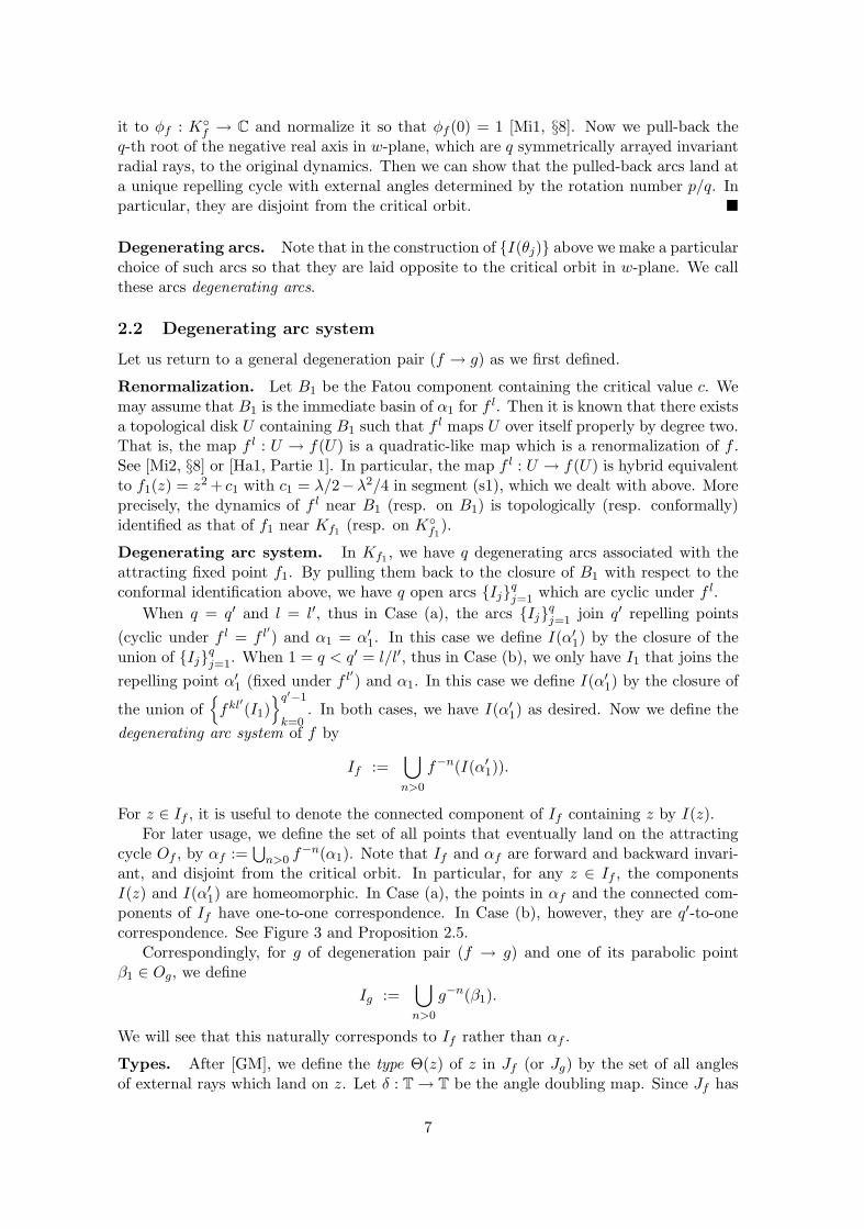
Figure 3: Left, the Julia set of an f in segment (s2) for p/q = 1/3, and right, one in segment(s1), with their degenerating arc system roughly drawn in. Attracting cycles are shownin heavy dots. Degenerating arcs with types {1/7, 2/7/4/7} and {1/28, 23/28, 25/28} areemphasized.

no critical points, one can easily see that δ(Θ(z)) coincides with Θ(f(z)). The same holdsfor g. Now a fact originally due to Thurston implies:

Lemma 2.4 For any point z in Jf or Jg, the set Θ(z) consists of finitely many angles.

See [Ki] for a generalized statement and the proof.We abuse the notation Θ(·) like this: For any subset E of the filled Julia set, its type

Θ(E) is the set of angles of the external rays that land on E. For each ζ in αf , we formallydefine the type of ζ by Θ(ζ) := Θ(I(ζ)). Then one can easily see that δn(Θ(ζ)) = Θ(α1)for some n > 0. We also set Θf := Θ(If ) and Θg := Θ(Ig). We will show that Θf equalsto Θg in the next proposition.

Valence. For any ζ ∈ αf , the component I(ζ) of If is univalently mapped onto I(α1)by iteration of f . Thus the value val(f) := card(Θ(ζ)) is a constant for f . Similarly, sincea small neighborhood of ξ in Ig is sent univalently over β1 by iteration of g, the valueval(g) := card(Θ(ξ)) is constant for g. Now we claim:

Proposition 2.5 For any degeneration pair (f → g), we have Θf = Θg and val(f) =val(g). Moreover,

• if q = q′ = 1 and l = l′ > 1 (thus Case (a) and non-trivial primitive), then val(g) = 2.

• Otherwise val(g) = q′.

We call val(f) = val(g) the valence of (f → g). Note that the valence depends only on g.

Proof. The two possibilities of val(g) above is shown in [Mi2, Lemma 2.7, §6]. If weshow that Θ(α′

1) = Θ(β1), then Θf = Θg and val(f) = val(g) automatically follow.

Case (a): q = q0. (Recall that in this case we have l = l′ and α1 = α′1.) First we

consider the case of q = q′ = 1. In this case by the argument of [Mi2, Theorem 4.1] thereexists a repelling cycle {γ1, . . . , γl′} of f satisfying γj′ → βj′ as f → g and Θ(γj′) = Θ(βj′)for j′ = 1, . . . , l′. Take the degenerating arc {I1} in the construction of If . Then I1 joinsα1(= α′

1) and γ1 thus Θ(α′1) = Θ(I(α1)) = Θ(γ1) = Θ(β1).

8

Next we consider the case of q = q′ > 1. When f is in segment (s1), the identityΘ(α′

1) = Θ(β1) is clear by Lemma 2.3. In the general case, we use renormalization.Let us take a path η in the parameter space joining c to σ according to the motion

as r → 1. By [Ha1, Theoreme 1], there is an analytic family of quadratic-like maps{f l

c′ : Uc′ → f lc′(Uc′)

}over a neighborhood of η such that the straightening maps are con-

tinuous and they give one-to-one correspondence between η and (s1).Let α1 ∈ Of and β1 ∈ Og be the attracting and parabolic fixed points of f l = f l

c :Uc → f l

c(Uc) and gl = f lσ : Uσ → f l

σ(Uσ) respectively, satisfying α1 → β1 as f → g. ByLemma 2.2, we can find q external rays landing at β1 in the original dynamics of g, whichis cyclic under gl. In particular, there are no more rays landing at β1 since such raysmust be cyclic of period q under gl and this contradicts [Mi2, Lemma 2.7]. Similarly inthe dynamics of f , by Lemma 2.3 and continuity of the straightening, there are exactlyq external rays of angles in Θ(β1) landing at q ends of I(α1) = I(α′

1). In fact, if there isanother ray of angle t /∈ Θ(β1) landing on such an end, then Rg(t) must land on β1 byorbit forcing ([Mi2, Lemma 7.1]). This is a contradiction. Thus Θ(α1) = Θ(α′

1) = Θ(β1).

Case (b): q = 1 < q0. By the argument of [Mi2, Theorem 4.1], the repelling pointsO′

f ={α′

1, . . . , α′l′}

must satisfy Θ(α′j′) = Θ(βj′) for j′ = 1, . . . , l′. �

In both Cases (a) and (b), it is convinient to assume that αj′ , αj′+l′ , . . . , αj′+(q′−1)l′

has the same types as that of βj′ for each j′ = 1, . . . , l′. Equivalently, we assume that

I(αj′) = I(αj′+l′) = · · · = I(αj′+(q′−1)l′)

throughout this papar.

2.3 Critical sectors

For ξ in Ig, the external rays of angles in Θ(ξ) cut the plane up into val(g) open regions,called sectors based at ξ. Similarly, for ζ in αf , the union of the external rays of anglesin Θ(ζ) and I(ζ) cut the plane up into val(f) = val(g) open regions. We abuse the termsectors based at I(ζ) for these regions.

Let B0 be the Fatou component of g that contains the critical point z = 0. Wemay ssume that β0 = βl′ is on the boundary of B0. Now one of the sectors based atβ0 contains the critical point 0, which is called the critical sector. For later usage, letθ+0 , θ

−0 ∈ R/Z denote the angles of external rays bounding the critical sector such that if

we take representatives θ+0 < θ−0 ≤ θ+

0 + 1 the external ray of angle θ with θ+0 < θ < θ−0

is contained in the critical sector. For example, we define θ+0 := 4/7 and θ−0 := 1/7 in

the case of Figure 3. In the case of Figure 8, we define θ+0 := 5/7 and θ−0 := 2/7. We

also define the critical sector based at I(α0) by one of the sector bounded by I(α0) andRf (θ±0 ).

3 Tessellation

In this section, we develop (and compactify) the method in [Ka2], and construct tessella-tion of the interior of the filled Julia sets for a degeneration pair (f → g).

For each θ ∈ Θf = Θg and some m ∈ Z (with a condition depending on θ), we willdefine the tiles Tf (θ,m,±) and Tg(θ,m,±) with the properties listed in Theorem 1.1. Theidea of tessellation is so simple as one can see in Figure 2, but we need to construct themprecisely to figure out their detailed combinatorial structure.

9

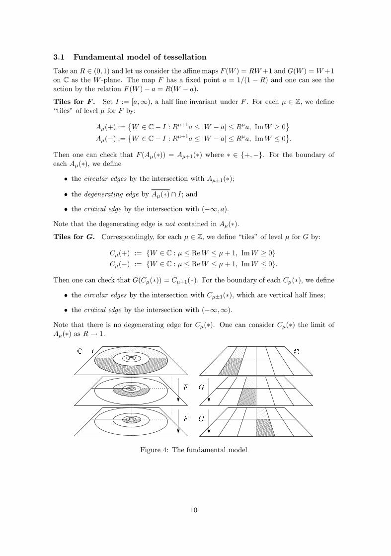
3.1 Fundamental model of tessellation

Take an R ∈ (0, 1) and let us consider the affine maps F (W ) = RW+1 and G(W ) = W+1on C as the W -plane. The map F has a fixed point a = 1/(1 − R) and one can see theaction by the relation F (W ) − a = R(W − a).

Tiles for F . Set I := [a,∞), a half line invariant under F . For each μ ∈ Z, we define“tiles” of level μ for F by:

Aμ(+) :={W ∈ C − I : Rμ+1a ≤ |W − a| ≤ Rμa, ImW ≥ 0

}Aμ(−) :=

{W ∈ C − I : Rμ+1a ≤ |W − a| ≤ Rμa, ImW ≤ 0

}.

Then one can check that F (Aμ(∗)) = Aμ+1(∗) where ∗ ∈ {+,−}. For the boundary ofeach Aμ(∗), we define

• the circular edges by the intersection with Aμ±1(∗);• the degenerating edge by Aμ(∗) ∩ I; and

• the critical edge by the intersection with (−∞, a).

Note that the degenerating edge is not contained in Aμ(∗).Tiles for G. Correspondingly, for each μ ∈ Z, we define “tiles” of level μ for G by:

Cμ(+) := {W ∈ C : μ ≤ ReW ≤ μ+ 1, ImW ≥ 0}Cμ(−) := {W ∈ C : μ ≤ ReW ≤ μ+ 1, ImW ≤ 0}.

Then one can check that G(Cμ(∗)) = Cμ+1(∗). For the boundary of each Cμ(∗), we define

• the circular edges by the intersection with Cμ±1(∗), which are vertical half lines;

• the critical edge by the intersection with (−∞,∞).

Note that there is no degenerating edge for Cμ(∗). One can consider Cμ(∗) the limit ofAμ(∗) as R→ 1.

Figure 4: The fundamental model

10

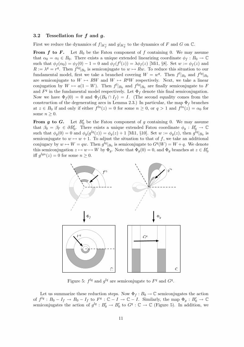
3.2 Tessellation for f and g.

First we reduce the dynamics of f |K◦f

and g|K◦g

to the dynamics of F and G on C.

From f to F . Let B0 be the Fatou component of f containing 0. We may assumethat α0 = αl ∈ B0. There exists a unique extended linearizing coordinate φf : B0 → C

such that φf (α0) = φf (0) − 1 = 0 and φf (f l(z)) = λφf (z) [Mi1, §8]. Set w := φf (z) andR := λq = rq. Then f lq|B0 is semiconjugate to w �→ Rw. To reduce this situation to ourfundamental model, first we take a branched covering W = wq. Then f l|B0 and f lq|B0

are semiconjugate to W �→ RW and W �→ RqW respectively. Next, we take a linearconjugation by W �→ a(1 − W ). Then f l|B0 and f lq|B0 are finally semiconjugate to Fand F q in the fundamental model respectively. Let Φf denote this final semiconjugation.Now we have Φf (0) = 0 and Φf (B0 ∩ If ) = I. (The second equality comes from theconstruction of the degenerating arcs in Lemma 2.3.) In particular, the map Φf branchesat z ∈ B0 if and only if either f ln(z) = 0 for some n ≥ 0, or q > 1 and f ln(z) = α0 forsome n ≥ 0.

From g to G. Let B′0 be the Fatou component of g containing 0. We may assume

that β0 = βl′ ∈ ∂B′0. There exists a unique extended Fatou coordinate φg : B′

0 → C

such that φg(0) = 0 and φg(glq(z)) = φg(z) + 1 [Mi1, §10]. Set w := φg(z), then glq|B0 issemiconjugate to w �→ w + 1. To adjust the situation to that of f , we take an additionalconjugacy by w �→W = qw. Then glq|B0 is semiconjugate to Gq(W ) = W + q. We denotethis semiconjugation z �→ w �→W by Φg. Note that Φg(0) = 0, and Φg branches at z ∈ B′

0

iff glqn(z) = 0 for some n ≥ 0.

Figure 5: f lq and glq are semiconjugate to F q and Gq.

Let us summarize these reduction steps. Now Φf : B0 → C semiconjugates the actionof f lq : B0 − If → B0 − If to F q : C − I → C − I. Similarly, the map Φg : B′

0 → C

semiconjugates the action of glq : B′0 → B′

0 to Gq : C → C (Figure 5). In addition, we

11

have one important property as follows:

Proposition 3.1 The branched linearization Φf do not ramify over C − (−∞, 0] or C −(−∞, 0]∪{a} according to q = 1 or q > 1. Similarly, the branched linearization Φg do notramify over C − (−∞, 0]. In particular, both Φf and Φg do not ramify over tiles of levelμ > 0.

See Theorem 5.5 for another important property of Φf and Φg.

Definition of tiles. A subset T ⊂ K◦f is a tile for f if there exist n ∈ N and μ ∈ Z

such that fn(T ) is contained in B0 and Φf ◦ fn maps T homeomorphically onto Aμ(+) orAμ(−). We define circular, degenerating, and critical edges for T by their correspondingedges of Aμ(±). We call the collection of such tiles the tessellation of K◦

f − If , and denoteit by Tess(f). In fact, one can easily check that

K◦f − If =

⋃T∈Tess(f)

T

and each z ∈ K◦f − If is either in the interior of an unique T ∈ Tess(f); a vertex shared

by four or eight tiles in Tess(f) if fm(z) = fn(0) for some n,m > 0; or on an edge sharedby two tiles in Tess(f) otherwise.

Tiles for g and tessellation of K◦g − Ig = K◦

g are also defined by replacing f , B0, andAμ(±) by g, B′

0, and Cμ(±) respectively.

Addresses. Each tile is identified by an address, which consists of an angle, a level, anda signature defined as followings:

Level and signature. For T ∈ Tess(f) above, i.e., fn(T ) ⊂ B0 and Φf ◦fn(T ) = Aμ(∗)with ∗ = + or −, we say that T has level m = μl − n and signature ∗. Then the criticalpoint z = 0 is a vertex of eight tiles of level 0 and −l.

For a tile T ′ ∈ Tess(g), its level and signature is defined in the same way.

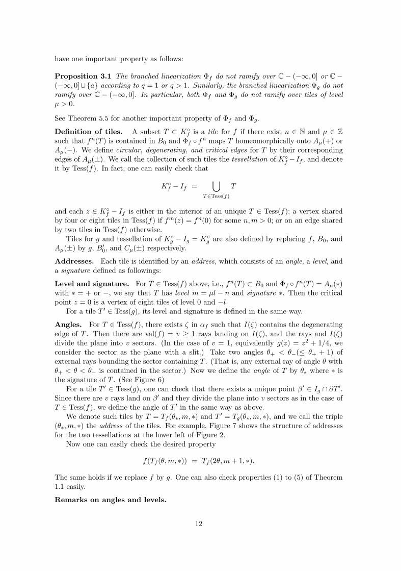
Angles. For T ∈ Tess(f), there exists ζ in αf such that I(ζ) contains the degeneratingedge of T . Then there are val(f) = v ≥ 1 rays landing on I(ζ), and the rays and I(ζ)divide the plane into v sectors. (In the case of v = 1, equivalently g(z) = z2 + 1/4, weconsider the sector as the plane with a slit.) Take two angles θ+ < θ−(≤ θ+ + 1) ofexternal rays bounding the sector containing T . (That is, any external ray of angle θ withθ+ < θ < θ− is contained in the sector.) Now we define the angle of T by θ∗ where ∗ isthe signature of T . (See Figure 6)

For a tile T ′ ∈ Tess(g), one can check that there exists a unique point β′ ∈ Ig ∩ ∂T ′.Since there are v rays land on β′ and they divide the plane into v sectors as in the case ofT ∈ Tess(f), we define the angle of T ′ in the same way as above.

We denote such tiles by T = Tf (θ∗,m, ∗) and T ′ = Tg(θ∗,m, ∗), and we call the triple(θ∗,m, ∗) the address of the tiles. For example, Figure 7 shows the structure of addressesfor the two tessellations at the lower left of Figure 2.

Now one can easily check the desired property

f(Tf (θ,m, ∗)) = Tf (2θ,m+ 1, ∗).

The same holds if we replace f by g. One can also check properties (1) to (5) of Theorem1.1 easily.

Remarks on angles and levels.

12

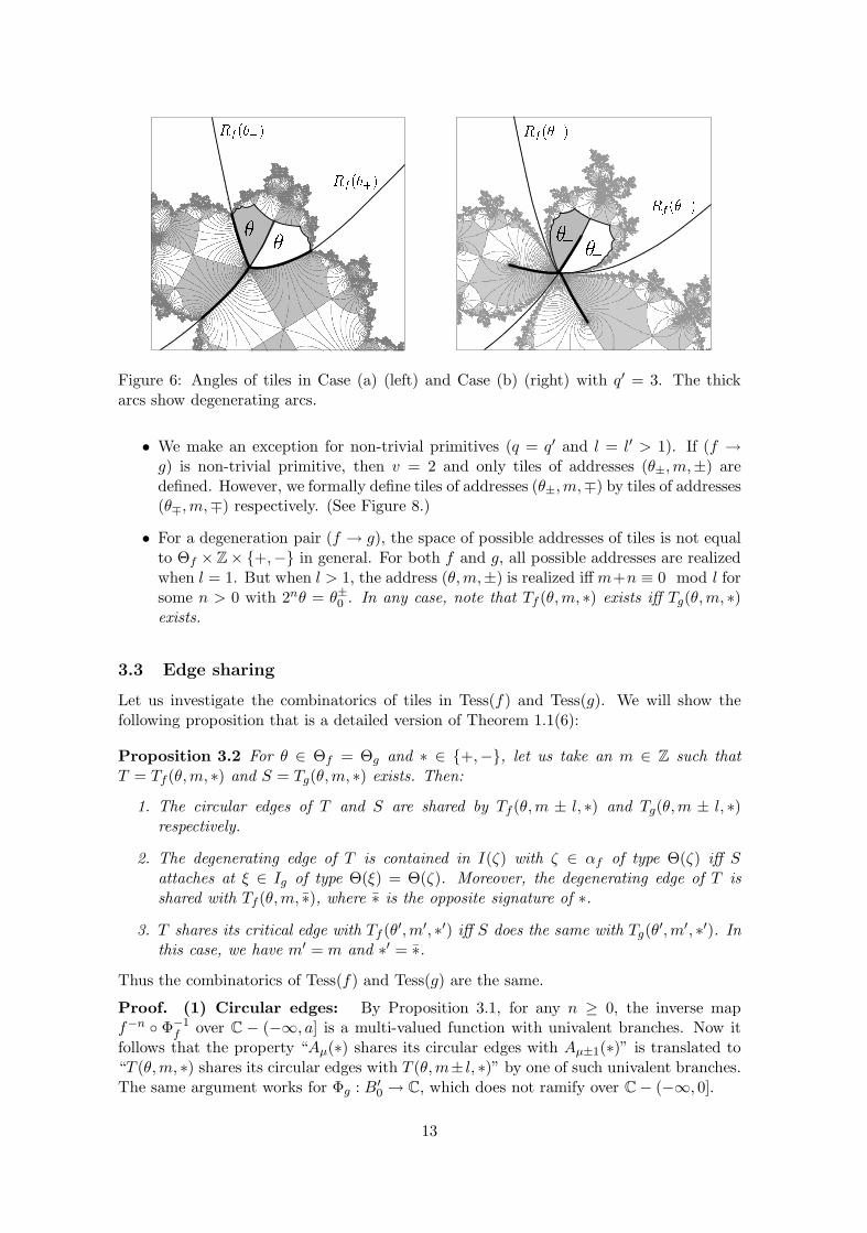
Figure 6: Angles of tiles in Case (a) (left) and Case (b) (right) with q′ = 3. The thickarcs show degenerating arcs.

• We make an exception for non-trivial primitives (q = q′ and l = l′ > 1). If (f →g) is non-trivial primitive, then v = 2 and only tiles of addresses (θ±,m,±) aredefined. However, we formally define tiles of addresses (θ±,m,∓) by tiles of addresses(θ∓,m,∓) respectively. (See Figure 8.)

• For a degeneration pair (f → g), the space of possible addresses of tiles is not equalto Θf × Z × {+,−} in general. For both f and g, all possible addresses are realizedwhen l = 1. But when l > 1, the address (θ,m,±) is realized iff m+n ≡ 0 mod l forsome n > 0 with 2nθ = θ±0 . In any case, note that Tf (θ,m, ∗) exists iff Tg(θ,m, ∗)exists.

3.3 Edge sharing

Let us investigate the combinatorics of tiles in Tess(f) and Tess(g). We will show thefollowing proposition that is a detailed version of Theorem 1.1(6):

Proposition 3.2 For θ ∈ Θf = Θg and ∗ ∈ {+,−}, let us take an m ∈ Z such thatT = Tf (θ,m, ∗) and S = Tg(θ,m, ∗) exists. Then:

1. The circular edges of T and S are shared by Tf (θ,m ± l, ∗) and Tg(θ,m ± l, ∗)respectively.

2. The degenerating edge of T is contained in I(ζ) with ζ ∈ αf of type Θ(ζ) iff Sattaches at ξ ∈ Ig of type Θ(ξ) = Θ(ζ). Moreover, the degenerating edge of T isshared with Tf (θ,m, ∗), where ∗ is the opposite signature of ∗.

3. T shares its critical edge with Tf (θ′,m′, ∗′) iff S does the same with Tg(θ′,m′, ∗′). Inthis case, we have m′ = m and ∗′ = ∗.

Thus the combinatorics of Tess(f) and Tess(g) are the same.

Proof. (1) Circular edges: By Proposition 3.1, for any n ≥ 0, the inverse mapf−n ◦ Φ−1

f over C − (−∞, a] is a multi-valued function with univalent branches. Now itfollows that the property “Aμ(∗) shares its circular edges with Aμ±1(∗)” is translated to“T (θ,m, ∗) shares its circular edges with T (θ,m± l, ∗)” by one of such univalent branches.The same argument works for Φg : B′

0 → C, which does not ramify over C − (−∞, 0].

13

5/24

5/24

5/24

1/6

1/61/6

1/12

1/121/12

11/12

11/1211/12

5/6

5/6 5/6

19/24

19/24

17/24

17/24

2/3

2/3

-1

-1

-1

-2

-2

-2

-2

-2

-2

-2

-2

-3

-3

-3

-3

-3

-3

-3

-3

-3

-3

-2

-2 -2

-200

0 0

1 1

1

2 0 0 0 0

-4

-4 -4

-4 -4

-4 -5

-5 -5

-5

-5

-5

-5

-5

-5

-5

-5

-5

-5

-5

-5

-5 -7

-7

-7

-7 -7

-7 -7

-7

-5 -5

-5

-5

-4 -4

-4

-4

-4

-4 -6 -8

-8-8

-8

-6 -6

-6

-4 -4

-4 -4

2 -1 -1

-1-1

-3

-3

-5

-5 -5

-5

-1 -1

-1

2/3

7/12

7/127/12

5/12

5/125/12

1/3

1/31/3

7/24

7/24

17/24 19/24

7/24

+

+-

-

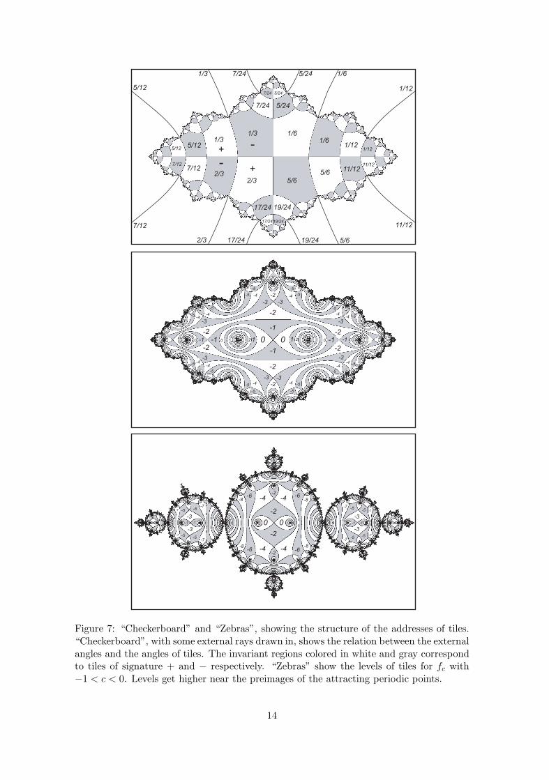
Figure 7: “Checkerboard” and “Zebras”, showing the structure of the addresses of tiles.“Checkerboard”, with some external rays drawn in, shows the relation between the externalangles and the angles of tiles. The invariant regions colored in white and gray correspondto tiles of signature + and − respectively. “Zebras” show the levels of tiles for fc with−1 < c < 0. Levels get higher near the preimages of the attracting periodic points.

14

2/73/7

4/75/7 6/7

1/72/7

5/7

(2/7, m, -)

(5/7, m, +)

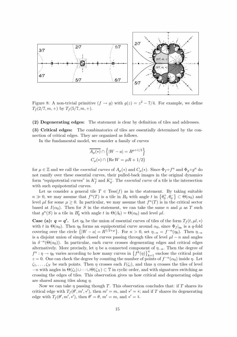
Figure 8: A non-trivial primitive (f → g) with g(z) = z2 − 7/4. For example, we defineTf (2/7,m,+) by Tf (5/7,m,+).

(2) Degenerating edges: The statement is clear by definition of tiles and addresses.

(3) Critical edges: The combinatorics of tiles are essentially determined by the con-nection of critical edges. They are organized as follows.

In the fundamental model, we consider a family of curves

Aμ(∗) ∩{|W − a| = Rμ+1/2

}

Cμ(∗) ∩ {ReW = μR+ 1/2}

for μ ∈ Z and we call the essential curves of Aμ(∗) and Cμ(∗). Since Φf ◦fn and Φg ◦gn donot ramify over these essential curves, their pulled-back images in the original dynamicsform “equipotential curves” in K◦

f and K◦g . The essential curve of a tile is the intersection

with such equipotential curves.Let us consider a general tile T ∈ Tess(f) as in the statement. By taking suitable

n � 0, we may assume that fn(T ) is a tile in B0 with angle t in{θ+0 , θ

−0

} ⊂ Θ(α0) andlevel μl for some μ ≥ 0. In particular, we may assume that fn(T ) is in the critical sectorbased at I(α0). Then for S in the statement, we can take the same n and μ as T suchthat gn(S) is a tile in B′

0 with angle t in Θ(β0) = Θ(α0) and level μl.

Case (a): q = q0. Let η0 be the union of essential curves of tiles of the form Tf (t, μl, ∗)with t in Θ(α0). Then η0 forms an equipotential curve around α0, since Φf |η0 is a q-foldcovering over the circle

{|W − a| = R1/2+μ}. For n > 0, set η−n = f−n(η0). Then η−n

is a disjoint union of simple closed curves passing through tiles of level μl − n and anglesin δ−n(Θ(α0)). In particular, each curve crosses degenerating edges and critical edgesalternatively. More precisely, let η be a connected component of η−n. Then the degree offn : η → η0 varies according to how many curves in

{fk(η)

}n

k=1enclose the critical point

z = 0. One can check the degree by counting the number of points of f−n(α0) inside η. Letζ1, . . . , ζN be such points. Then η crosses each I(ζi), and thus η crosses the tiles of level−n with angles in Θ(ζ1)∪· · ·∪Θ(ζN) ⊂ T in cyclic order, and with signatures switching ascrossing the edges of tiles. This observation gives us how critical and degenerating edgesare shared among tiles along η.

Now we can take η passing though T . This observation concludes that: if T shares itscritical edge with Tf (θ′,m′, ∗′), then m′ = m, and ∗′ = ∗; and if T shares its degeneratingedge with Tf (θ′,m′, ∗′), then θ′ = θ, m′ = m, and ∗′ = ∗.

15

For S, consider a circle around β0 which is so small that the circle and the essentialcurves of tiles with angle θ ∈ Θ(β0) and level μl bound a flower-like disk (Figure 9). Letus denote the boundary of the disk by η′0, which works as η0. Since the combinatorics ofpulled-back sectors based at β0 and I(α0) is the same, the observation of g−n(η′0) = η′−n

must be the same as that of η−n. This concludes the statement.

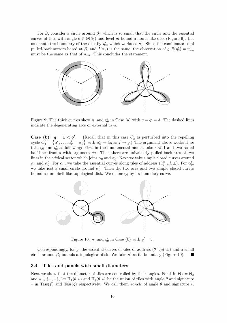
Figure 9: The thick curves show η0 and η′0 in Case (a) with q = q′ = 3. The dashed linesindicate the degenerating arcs or external rays.

Case (b): q = 1 < q0. (Recall that in this case Og is perturbed into the repellingcycle O′

f ={α′

1, . . . , α′l′ = α′

0

}with α′

0 → β0 as f → g.) The argument above works if wetake η0 and η′0 as following: First in the fundamental model, take ε � 1 and two radialhalf-lines from a with argument ±ε. Then there are univalently pulled-back arcs of twolines in the critical sector which joins α0 and α′

0. Next we take simple closed curves aroundα0 and α′

0. For α0, we take the essential curves along tiles of address (θ±0 , μl,±). For α′0,

we take just a small circle around α′0. Then the two arcs and two simple closed curves

bound a dumbbell-like topological disk. We define η0 by its boundary curve.

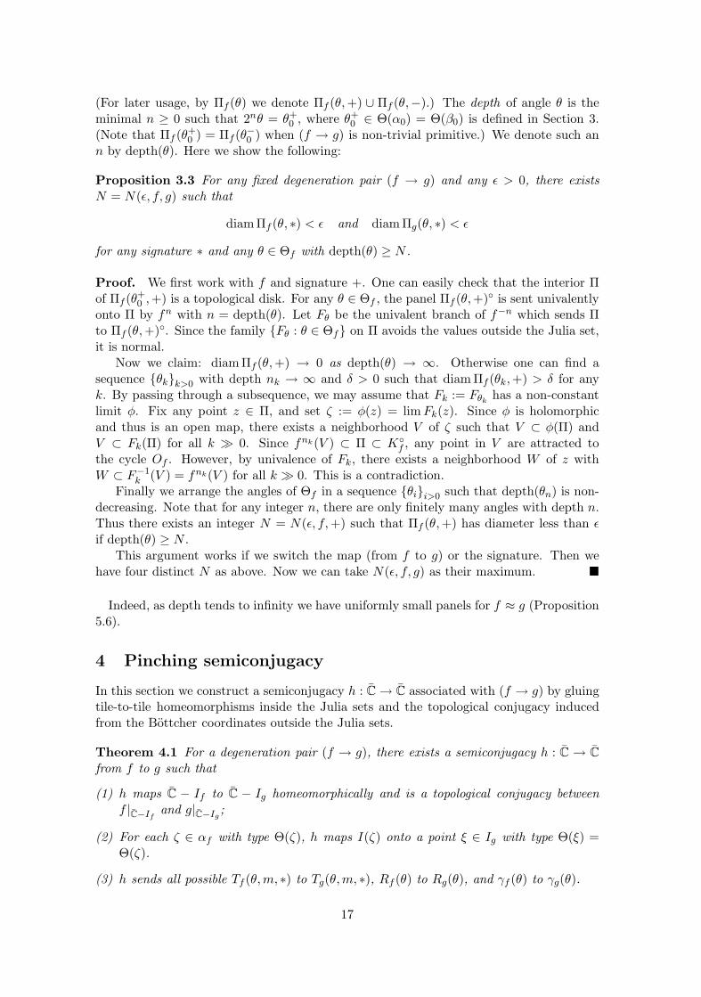
Figure 10: η0 and η′0 in Case (b) with q′ = 3.

Correspondingly, for g, the essential curves of tiles of address (θ±0 , μl,±) and a smallcircle around β0 bounds a topological disk. We take η′0 as its boundary (Figure 10). �

3.4 Tiles and panels with small diameters

Next we show that the diameter of tiles are controlled by their angles. For θ in Θf = Θg

and ∗ ∈ {+,−}, let Πf (θ, ∗) and Πg(θ, ∗) be the union of tiles with angle θ and signature∗ in Tess(f) and Tess(g) respectively. We call them panels of angle θ and signature ∗.

16

(For later usage, by Πf (θ) we denote Πf (θ,+) ∪ Πf (θ,−).) The depth of angle θ is theminimal n ≥ 0 such that 2nθ = θ+

0 , where θ+0 ∈ Θ(α0) = Θ(β0) is defined in Section 3.

(Note that Πf (θ+0 ) = Πf (θ−0 ) when (f → g) is non-trivial primitive.) We denote such an

n by depth(θ). Here we show the following:

Proposition 3.3 For any fixed degeneration pair (f → g) and any ε > 0, there existsN = N(ε, f, g) such that

diam Πf (θ, ∗) < ε and diam Πg(θ, ∗) < ε

for any signature ∗ and any θ ∈ Θf with depth(θ) ≥ N .

Proof. We first work with f and signature +. One can easily check that the interior Πof Πf (θ+

0 ,+) is a topological disk. For any θ ∈ Θf , the panel Πf (θ,+)◦ is sent univalentlyonto Π by fn with n = depth(θ). Let Fθ be the univalent branch of f−n which sends Πto Πf (θ,+)◦. Since the family {Fθ : θ ∈ Θf} on Π avoids the values outside the Julia set,it is normal.

Now we claim: diam Πf (θ,+) → 0 as depth(θ) → ∞. Otherwise one can find asequence {θk}k>0 with depth nk → ∞ and δ > 0 such that diam Πf (θk,+) > δ for anyk. By passing through a subsequence, we may assume that Fk := Fθk

has a non-constantlimit φ. Fix any point z ∈ Π, and set ζ := φ(z) = limFk(z). Since φ is holomorphicand thus is an open map, there exists a neighborhood V of ζ such that V ⊂ φ(Π) andV ⊂ Fk(Π) for all k � 0. Since fnk(V ) ⊂ Π ⊂ K◦

f , any point in V are attracted tothe cycle Of . However, by univalence of Fk, there exists a neighborhood W of z withW ⊂ F−1

k (V ) = fnk(V ) for all k � 0. This is a contradiction.Finally we arrange the angles of Θf in a sequence {θi}i>0 such that depth(θn) is non-

decreasing. Note that for any integer n, there are only finitely many angles with depth n.Thus there exists an integer N = N(ε, f,+) such that Πf (θ,+) has diameter less than εif depth(θ) ≥ N .

This argument works if we switch the map (from f to g) or the signature. Then wehave four distinct N as above. Now we can take N(ε, f, g) as their maximum. �

Indeed, as depth tends to infinity we have uniformly small panels for f ≈ g (Proposition5.6).

4 Pinching semiconjugacy

In this section we construct a semiconjugacy h : C → C associated with (f → g) by gluingtile-to-tile homeomorphisms inside the Julia sets and the topological conjugacy inducedfrom the Bottcher coordinates outside the Julia sets.

Theorem 4.1 For a degeneration pair (f → g), there exists a semiconjugacy h : C → C

from f to g such that

(1) h maps C − If to C − Ig homeomorphically and is a topological conjugacy betweenf |C−If

and g|C−Ig;

(2) For each ζ ∈ αf with type Θ(ζ), h maps I(ζ) onto a point ξ ∈ Ig with type Θ(ξ) =Θ(ζ).

(3) h sends all possible Tf (θ,m, ∗) to Tg(θ,m, ∗), Rf (θ) to Rg(θ), and γf (θ) to γg(θ).

17

This theorem emphasizes the combinatorial property of h. In the next section we willshow that h→ id as f uniformly tends to g.

Trans-component partial conjugacy and subdivision of tessellation. Let (f1 →g1) and (f2 → g2) be distinct satellite degeneration pair with g1 = g2. More precisely, weconsider (f1 → g1) and (f2 → g2) are tuned copy of degeneration pairs in segment (s1)and (s2) with q > 1 by the same tuning operator. By composing homeomorphic parts ofthe conjugacies associated with (f1 → g1) and (f2 → g2), we have:

Corollary 4.2 There exists a topological conjugacy κ = κf1,f2 : C − If1 → C − If2 fromf1 to f2.

For example, the panel Πf1(θ, ∗) is mapped to the panel Πf2(θ, ∗). Now we can compareTess(f1) and Tess(f2) via Tess(gi). By comparing Tess(g1) and Tess(g2), one can easilycheck that

Tg2(θ, μ, ∗) =q−1⋃j=0

Tg1(θ, μ+ lj, ∗)

for any Tg2(θ, μ, ∗) ∈ Tess(g2). Thus Tess(g1) is just a subdivision of Tess(g2).Take a tile Tf1(θ,m, ∗) ∈ Tess(f1). Then there is a homeomorphic image T ′

2(θ,m, ∗) :=κ(Tf1(θ,m, ∗)) in K◦

f2. We say the family

Tess′(f2) := {κ(T ) : T ∈ Tess(f1)}is the subdivided tessellation of K◦

f2− If2. Since Tess(f1) and Tess(f2) have the same

combinatorics as Tess(g1) and Tess(g2) respectively,

Tf2(θ, μ, ∗) =q−1⋃j=0

T ′f2

(θ, μ+ lj, ∗)

for any Tf2(θ, μ, ∗) ∈ Tess(f2). Now we have a natural tile-to-tile correspondence betweenTess(f1), Tess(g1) and Tess′(f2). In other word, combinatorial property of tessellation ispreserved under the degeneration from f1 to g and the bifurcation from g to f2.

In Part II of this paper, we will use this property to investigate the structure of theLyubich-Minsky hyperbolic 3-laminations associated with f1, g, and f2.

4.1 Proof of Theorem 4.1

The rest of this section is devoted to the proof of the theorem. The proof breaks into fivesteps.

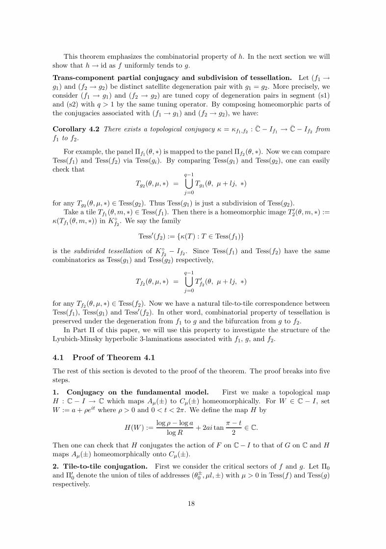
1. Conjugacy on the fundamental model. First we make a topological mapH : C − I → C which maps Aμ(±) to Cμ(±) homeomorphically. For W ∈ C − I, setW := a+ ρeit where ρ > 0 and 0 < t < 2π. We define the map H by

H(W ) :=log ρ− log a

logR+ 2ai tan

π − t

2∈ C.

Then one can check that H conjugates the action of F on C− I to that of G on C and Hmaps Aμ(±) homeomorphically onto Cμ(±).

2. Tile-to-tile conjugation. First we consider the critical sectors of f and g. Let Π0

and Π′0 denote the union of tiles of addresses (θ±0 , μl,±) with μ > 0 in Tess(f) and Tess(g)

respectively.

18

Figure 11: H maps A0(+) to C0(+).

By Proposition 3.1, the map Φf : Π0 → C is univalent and we can choose a univalentbranch Ψg of Φ−1

g which sends {W : ReW ≥ 1} to Π′0. For each point in Π0, we define

h := Ψg ◦ H ◦ Φf |Π0 . Then we have a conjugacy between f lq|Π0 and glq|Π′0. Any tile

eventually lands on tiles in Π0 or Π′0. According to the combinatorics of tiles determined

by pulling-back essential curves in Π0 and Π′0, we can pull-back h over K◦

f − If andh : K◦

f − If → K◦g is a conjugacy.

3. Continuous extension to degenerating arc system. Take any ζ ∈ αf . For anypoint z in I(ζ), we define h(z) by the unique ξ ∈ Ig with Θ(ξ) = Θ(ζ).

Now we show the continuity of h : K◦f ∪ If → K◦

g ∪ Ig which we have defined. Take anyz in I(ζ). We claim that any sequence zn ∈ K◦

f ∪ If converging to z satisfies h(zn) → ξ.First when z is neither ζ nor one of the endpoints of I(ζ), it is enough to consider the

case of zn ∈ K◦f −If for all n. Now z is on the degenerating edges of at most four tiles. Let

T = Tf (θ,m,+) be one of such tiles. The subsequence zni of zn contained in T is mappedto Tg(θ,m,+). In the fundamental model, the sequence h(zni) corresponds to a sequencewhose imaginary part is getting higher. Thus h(zni) converges to ξ with type containingθ, which must coincide with Θ(ζ). By changing the choice of T , we have h(zn) → ξ withΘ(ξ) = Θ(ζ).

Next, if z is ζ or one of the endpoints of I(ζ), it is an attracting or repelling periodicpoint. If z is attracting, the levels of tiles containing zn go to +∞. According to thefundamental model, we have h(zn) → ξ.

The last case is when z is repelling, thus in the Julia set. We deal with this case inthe next paragraph.

4. Continuous extension to the Julia set. Take any z ∈ Jf and any sequencezn ∈ K◦

f ∪ If converging to z. Then we take a sequence θn ∈ Θf such that zn ∈ Πf (θn).After passing to a subsequence we may assume θn and h(zn) converge to some θ ∈ T andw ∈ Kg respectively.

We first claim that z = γf (θ), that is, θ ∈ Θ(z). If the depth of θn is bounded, thenθn = θ ∈ Θf for all n � 0. This implies zn ∈ Πf (θ) for all n � 0 and it follows thatz ∈ Πf (θ) ∩ Jf . Thus z = γf (θ) by definition of Πf (θ). If the depth of θn is unbounded,it is enough to consider the subsequences with the depth of θn monotonously increasing.Take any ε > 0. For n� 0, we have |γf (θn)−zn| < ε by Proposition 3.3, and we also have|γf (θn) − γf (θ)| < ε by continuity of γf : T → Jf . Finally |z − zn| < ε for n � 0 implies|z − γf (θ)| < 3ε and conclude the claim.

Since h(zn) ∈ Πg(θn), the same argument works for h(zn) and w. Hence we also claimthat w = γg(θ) ∈ Jg. It follows that the original zn → z implies h(zn) accumulates only

19

on γg(θ) with θ ∈ Θ(z).By Theorem A.1, there exists a semiconjugacy hJ : Jf → Jg with hJ ◦ γf = γg. Since

γf (θ) = γf (θ′) for any θ and θ′ in Θ(z), we have γg(θ) = γg(θ′). This implies that h(zn)accumulates on a unique point γg(θ). Thus h continuously extends to the Julia set byh(γf (θ)) := γg(θ) for each θ ∈ T.

5. Global extension. Finally we define h : C−Kf → C−Kg by the conformal conjugacybetween f |C−Kf

and g|C−Kggiven via Bottcher coordinates. This conjugacy and the

semiconjugacy above continuously glued along the Julia set thus we have a semiconjugacyon the sphere.

Properties (2) and (3) are clear by construction. To check property (1), we need toshow that h−1 : C − If → C − Ig is continuous. Continuity in C −Kg and K◦

g is obviousby construction. Take any point w ∈ Jg − Ig. A similar argument to step 4 shows thatany sequence wn → w within C − Ig is mapped to a convergent sequence zn → z withinC − If satisfying Θ(z) = Θ(w) ⊂ T − Θg. �

5 Continuity of pinching semiconjugacies

In this section we deal with continuity of the dynamics of the degeneration pair (f → g)as f tends to g. We will establish:

Theorem 5.1 Let h : C → C be the semiconjugacy associated with a degeneration pair(f → g) that is given in Theorem 4.1. Then h tends to identity as f tends to g.

Here are two immediate corollaries:

Corollary 5.2 The closures of Tf (θ,m, ∗) and Πf (θ, ∗) in Tess(f) uniformly converge tothose of Tg(θ,m, ∗) and Πg(θ, ∗) in Tess(g) in the Hausdorff topology.

Corollary 5.3 As f → g, the diameters of connected components of If uniformly tendsto 0.

Let us start with some terminologies for the proof. Two degeneration pair (f1 → g1)and (f2 → g2) are equivalent if g1 = g2 and both f1 and f2 are in the same hyperboliccomponent. For a degeneration pair (f → g) by f ≈ g we mean f is sufficiently close tog. In other words, the multiplier rω of Of is sufficiently close to ω, i.e., r ≈ 1.

Formally we consider a family of equivalent degeneration pairs {(f → g)} parameter-ized by 0 < r < 1 and its behavior when r tends to 1. To show the theorem, it suffices toshow the following:

(i) For any compact set K in C−Kg, we have K ⊂ C−Kf for all f ≈ g and h→ id onK.

(ii) For any compact set K in K◦g , we have K ⊂ K◦

f for all f ≈ g and h→ id on K.

(iii) h is equicontinuous as f → g on the sphere.

In fact, any sequence hk associated with fk → g has a subsequential limit h∞ whichis identity on C − Jg and continuous on C. Since C − Jg is open and dense, the map h∞must be identity on the whole sphere.

20

5.1 Proof of (i)

Let Bf : C − D → C −K◦f be the extended Bottcher coordinate of Kf , i.e., Bf : C − D →

C − Kf is a conformal map with Bf (w2) = f(Bf (w)); Bf (w)/w → 1 as w → ∞; andBf (e2πiθ) := γf (θ) ∈ Jf . Now (i) follows immediately from this stronger claim:

Theorem 5.4 (Bottcher convergence) As f → g, we have a uniform convergenceBf → Bg on C − D.

Note that the uniform convergence on compact sets in C− D is not difficult. Our proof isa mild generalization of the proof of Theorem 2.11 in [Po].

Proof. By Corollary A.2 one can easily check that C −Kf converges to C −Kg in thesense of Caratheodory kernel convergence with respect to ∞. Thus pointwise convergenceBf → Bg on each z ∈ C − D is given by [Po, Theorem 1.8] and B′

f (∞) = B′g(∞) = 1. To

show the theorem, it is enough to show that Kf is uniformly locally connected as f → gby [Po, Corollary 2.4]. That is, for any ε > 0, there exists δ > 0 such that for any f ≈ gand any a, b ∈ Kf with |a− b| < δ, there exists a continuum E such that diamE < ε.

Suppose we have a sequence of equivalent degenerating pairs (fn → g) such that:fn → g uniformly; for fn there exist an and a′n in Jfn with |an − a′n| → 0 which cannot be contained in the same continuum in Kfn of diameter less than ε0 > 0. We mayset an = γfn(θn) and a′n = γfn(θ′n) for some θn, θ

′n ∈ T since γfn maps T onto Jfn .

By passing to a subsequence, we may also assume that θn → θ and θ′n → θ′. Sinceγfn → γg uniformly by Corollary A.3, the assumption |an − a′n| → 0 implies that we haveγg(θ) = γg(θ′) =: w ∈ Jg.

Case 1: θ = θ′. We may assume that θn ≤ θ′n and both tend to θ. Set En :={γfn(t) : t ∈ [θn, θ

′n]}, which is a continuum containing an and a′n. Then for any t ∈ [θn, θ

′n],

we have |γfn(t)−w| ≤ |γfn(t)− γg(t)|+ |γg(t)− γg(θ)| → 0 since γfn → γg uniformly andγg is continuous. This implies diamEn → 0 and is a contradiction.

Case 2-1: θ �= θ′ and w /∈ Ig. First we show that γfn(θ) = γfn(θ′). Let hn : Jfn → Jg bethe semiconjugacy given by Theorem A.1. Since hn ◦ γfn = γg, we have

w = hn ◦ γfn(θ) = hn ◦ γfn(θ′) /∈ Ig.

By property 1 of Theorem A.1, this implies γfn(θ) = γfn(θ′). Now set

En :={γfn(t) : |t− θ| ≤ |θn − θ| or |t− θ′| ≤ |θ′n − θ′|},

which is a continuum containing an and a′n. Again one can easily check that |γfn(t)−w| →0 uniformly for any γfn(t) ∈ En and diamEn → 0.

Case 2-2: θ �= θ′ and w ∈ Ig. There exists an m ≥ 0 such that gm(w) = β0. Sincehn ◦ γfn = γg we have γfn(θ), γfn(θ′) ∈ h−1

n (w) ⊂ Jfn ∩ Ifn . If q = 1, then hn is homeo-morphism by Theorem A.1. Thus γfn(θ) = γfn(θ′) and a contradiction follows from thesame argument as above.

Suppose q > 1. Then Case (a) (q = q′ and l = l′) by Proposition 2.1. In particular, wehave wn ∈ αfn such that wn → w and fm

n (wn) is an attracting periodic point α0,n ∈ Ofn

which tends to β0. Let λn = rne2πip/q be the multiplier of Ofn with rn ↗ 1. On a fixed

small neighborhood of w, we have

f−m ◦ f lq ◦ fm(z) = rqnz (1 + zq +O(z2q))

−→ g−m ◦ glq ◦ gm(z) = z (1 + zq +O(z2q))

21

by looking though suitable local coordinates as in Appendix A.2. (For simplicity, weabbreviate conjugations by the local coordinates.)

By Lemma A.7, we can find a small continuum E′n ⊂ Kfn which joins wn and preperi-

odic points γfn(θ), γfn(θ′). Set En as in Case 2-1. Now E′n∪En is a continuum containing

an and a′n. Since diam (E′n ∪ En) → 0, we have a contradiction again. �

5.2 Proof of (ii)

Let us start with the following theorem:

Theorem 5.5 (Linearization convergence) Let K be any compact set in K◦g . Then

K ⊂ K◦f for f ≈ g and Φf → Φg uniformly on K.

Proof. One can easily check that K ⊂ K◦f if f ≈ g by Corollary A.2. Let β0 ∈ Og ∩∂B′

0.We may assume that K ′ = gN (K) is sufficiently close to β0 and contained in B′

0 by takinga suitable N � 0. Then K ′ is attracted to β0 along the attracting direction associatedwith B′

0 by iteration of gl′q′ . For simplicity, set l := lq = l′q′.Recall that Φf and Φg semiconjugate f l and gl to F q and Gq in the fundamental model

respectively. We will construct other semiconjugacies Φf and Φg with the same propertyplus Φf → Φg on compact subsets of a small attracting petal in B′

0. Then we will showthat they coincide.

By Appendix A.2, there exist local coordinates ζ = ψf (z) and ζ = ψg(z) with ψf → ψg

near β0 such that we can view f l → gl as

f l(ζ) = Λζ (1 + ζq′ +O(ζ2q′))

−→ gl(ζ) = ζ (1 + ζq′ +O(ζ2q′))

where Λ→ 1. (To simplify notation, we abbreviate conjugations by these local coordinates.For example, by f l(ζ) we mean ψf ◦ f l ◦ ψ−1

f (ζ).) Now there are two cases for Λ:

• In Case (a) (q = q′ and l = l′), the fixed point ζ = 0 is attracting and Λ = λq =rq = R < 1.

• In Case (b) (q = 1 < q′ = l/l′), the fixed point ζ = 0 is repelling and |Λ| > 1.

Next by taking branched coordinate changes w = Ψf (ζ) = −Λq′/(q′ζq′) and w = Ψg(ζ) =−1/(q′ζq′) respectively, we can view f l → gl as

f l(w) = Λ−q′w + 1 +O(1/w)

−→ gl(w) = w + 1 +O(1/w).

Case (a). Set τ = Λ−q′ = R−q > 1. By simultaneous linearization in AppendixA.3, we have convergent coordinate changes W = uf (w) → ug(w) on compact sets ofPρ := {Rew > ρ� 0} such that f l → gl is viewed as

F (W ) := f l(W ) = τW + 1

−→ G(W ) := gl(W ) = W + 1.

Let us adjust F → G to F q → Gq in the fundamental model. Recall that the mapF (W ) = RW + 1 has the attracting fixed point at a = 1/(1−R). On the other hand, the

22

map F has the repelling fixed point a = 1/(1−R−q) instead. Set Tf (W ) := aW/(W − a).Then Tf (W ) = qW (1 + O(W/a)) → Tg(W ) = qW on any compact sets on the W -planeas R → 1. By taking conjugations with Tf and Tg, we can view F → G as F q → Gq onany compact sets of the domain of G.

Case (b). By Rouche’s theorem, there exists a fixed point b of f l(w) = Λ−q′w +1 + O(1/w) of the form b = 1/(1 − Λ−q′) + O(1). Indeed, this b is one of the image ofthe attracting cycle Of hence its multiplier is r < 1. Set Sf (w) := bw/(b − w). ThenSf (w) = w(1 + O(w/b)) → Sg(w) = w on any compact sets of w-plane as r → 1. Bytaking conjugations by Sf and Sg, we can view f l(w) → gl(w) as

f l(w) = τw + 1 +O(1/w)

−→ gl(w) = w + 1 +O(1/w)

where τ = 1/r > 1. By simultaneous linearization, we have convergent coordinate changesW = uf (w) → ug(w) on compact sets of Pρ such that f l → gl is again viewed as

F (W ) := f l(W ) = τW + 1

−→ G(W ) := gl(W ) = W + 1.

Since q = 1, we adjust F → G to F → G in the fundamental model. Set b := 1/(1−τ) andTf (W ) := bW/(b−W ). Then Tf (W ) = W (1 +O(W/b)) → Tg(W ) = W on any compactsets on the W -plane as r → 1. By taking conjugations by Tf and Tg, we can view F → Gas F → G on any compact sets of the domain of G.

Adjusting critical orbits. Now we denote these final local coordinates conjugatingf l → gl to F q → Gq by Φf → Φg, where the convergence holds on compact subsets of asmall attracting petal P ′ in B′

0 corresponding to Pρ in the w-plane.We need to adjust the positions of the images of the critical orbits on the W -plane by

Φf → Φg to those by Φf and Φg. We may assume that gnl(0) ∈ P ′ for fixed n� 0. Thenfnl(0) ∈ P ′ for all f ≈ g. Set s := Φf (fnl(0)) and s′ := Φg(gnl(0)). Then s→ s′ as f → g.On the other hand, we have

Φf (fnl(0)) = Fnq(Φf (0)) = Fnq(0) = Rnq−1 + · · · + 1 =: Rn

and Φg(gnl(0)) = nq. Set Uf (W ) := k(W − a) + a and Ug(W ) := W + nq − s′ wherek = (Rn − a)/(s − a). Then one can check that Uf → Ug on any compact sets in theW -plane as f → g and Uf and Ug commute with F and G respectively. By defining Φf

and Φg by Uf ◦ Φf and Ug ◦ Φg respectively, we have Φf → Φg on compact sets of P ′ withΦf (fnl(0)) = Rn and Φg(gnl(0)) = nq.

Finally we need to check that Φf = Φf and Φg = Φg. The latter equality is clear byuniqueness of the Fatou coordinate ([Mi1, §8]). For the former, recall that W = Φf (z) isgiven by

z �→ φf (z) = w �→ wq = W �→ a(1 −W ) =: Φf (z)

and φf is uniquely determined under the condition of φf (0) = 1 ([Mi1, §10]). Let usconsider the local coordinate φf on a compact set of P ′ given by

z �→ Φf (z) = W �→(

1 − W

a

)1/q

=: φf (z) = w,

23

where we take a suitable branch of qth root such that φf (fnl(0)) = λnq on the w-plane.Then φf (f(z)) = λφf (z). Since φf (0) = 1 is equivalent to φf (fnl(0)) = λnq, the map φf

coincide with φf . This implies the former equality.Now we may assume that K ′ = gN (K) ⊂ D � P ′ for some open set D. If f ≈ g, then

fN(K) ⊂ D and we have the uniform convergence Φg → Φf on D. We finally obtain theuniform convergence on K by Φf (z) = F−N (Φf (fN (z))) → G−N (Φg(gN (z)) = Φg(z) forz ∈ K. �

Proof of (ii). We first work with the fundamental model. Suppose ε ↘ 0, and setR = 1 − ε. Then F (W ) = RW + 1 fixes aε = 1/(1 − R) = ε−1. For a fixed γ with1/2 < γ < 1, we define a compact set Qε ⊂ C by:

Qε :={W = aε + ρe(π−t)i ∈ C : |t| ≤ εγ , |ρ− aε| ≤ aε sin εγ

}.

Let D be any bounded set in C. For all ε � 1, the compact set Qε contains D. LetH : C−[aε,∞) → C be the conjugacy between F and G(W ) = W+1 as in Section 4. Thenone can easily check that |ReW−ReH(W )| = O(ε2γ−1) and |ImW−ImH(W )| = O(ε2γ−1)on Qε. Thus H → id uniformly on D.

Let K be any compact set in K◦g , and let D be the 1/10-neighborhood of Φg(K). For

all f ≈ g, we have K ⊂ K◦f and Φf (K) ⊂ D by Theorem 5.5. By the argument above on

the fundamental model, the restriction h|K is a branch of Φ−1g ◦H ◦Φf that converges to

the identity. (The branch is determined by the tile-to-tile correspondence given by h.) �

5.3 Proof of (iii)

To show (iii) we need two propositions on properties of panels as f → g. The first one isa refinement of Proposition 3.3, and the second one is on the convergence of panels witha fixed angle:

Proposition 5.6 (Uniformly small panels) For any ε > 0, there exists N = N(ε)such that for all f ≈ g, ∗ = ± and θ ∈ Θg with depth(θ) ≥ N ,

diam Πf (θ, ∗) < ε and diam Πg(θ, ∗) < ε.

Proposition 5.7 (Hausdorff convergence to a panel) For fixed angle θ ∈ Θg andsignature ∗ = + or −, we have Πf (θ, ∗) → Πg(θ, ∗) as f → g in the Hausdorff topology.

Let us show (iii) first by assuming them:

Proof of (iii). By (i) we have equicontinuity near ∞. Assume that there exist degener-ation pairs (fk → g) with semiconjugacies hk as in Theorem 4.1, points ak, a

′k ∈ C with

|ak − ak| → 0, and bk = hk(ak), b′k = hk(a′k) with |bk − b′k| ≥ ε0 > 0.Suppose that ak, a

′k ∈ C−K◦

f thus bk, b′k ∈ C−K◦g . Then there exists wk, w

′k ∈ C−D

such that ak = Bfk(wk), a′k = Bfk

(w′k) and bk = Bg(wk), b′k = Bg(w′

k). By Theorem 5.4,we have Bfk

→ Bg. Thus |ak − a′k| → 0 implies |bk − b′k| → 0, a contradiction.Now it is enough to show the case where ak, a

′k ∈ Kfk

thus bk, b′k ∈ Kg. By takingsubsequences, we may assume that ak → a, a′k → a, bk → b, and b′k → b′ with |b − b′| ≥ε0/2 > 0. Since Kfk

→ Kg in the Hausdorff topology, a, b and b′ are all in Kg.First let us consider the case where a is bounded distance away from Jg. Then we have

a compact neighborhood E of a such that hk|E → id|E and ak, a′k ∈ E for all k � 0. This

implies that |bk − b′k| → 0, a contradiction.

24

Next we consider the case where a ∈ Jg. For ak → a and bk → b, we will claim thata = b. Then by the same argument we have a = b′ and this is a contradiction.

For ak ∈ Kfk, we take any θk ∈ T such that: ak = γfk

(θk) if ak ∈ Jfk; otherwise ak is

contained in the closure of Πfk(θk). (Then bk = γg(θk) or bk is in the closure of Πg(θk).)

By passing to a subsequence, we may assume that θk → θ for some θ ∈ T.If θk /∈ Θg, we define its depth by ∞. Then there are two more cases according to

lim supdepth(θk) = ∞ or not.If lim supdepth(θk) = ∞, we take a subsequence again and assume that depth(θk) is

strictly increasing. Then by Proposition 5.6 we have |ak − γfk(θk)| → 0. Since θk → θ and

γfk→ γg uniformly (Corollary A.3), we have |ak − γg(θ)| → 0, thus a = γg(θ). Similarly

we conclude that b = γg(θ) and this implies a contradiction.If lim supdepth(θk) < ∞, we take a subsequence again and assume that θk = θ ∈ Θg

for all k � 0. By Proposition 5.7 ak ∈ Πfk(θ) are approximated by some ck ∈ Πg(θ) with

|ak − ck| → 0 thus ck → a ∈ Jg. Since Πg(θ) ∩ Jg = {γg(θ)}, we have a = γg(θ). Onthe other hand, if bk ∈ Πg(θ) is bounded distance away from Jg, there exists a compactneighborhood E′ ⊂ K◦

g of b where hk|E′ → id|E′ and it leads to a contradiction. Thusb ∈ Jg and it must be γg(θ). Now we obtain a = b. �

To complete the proof of Theorem 5.1, let us finish the proofs of the propositions.

Proof of Proposition 5.6. We modify the argument of Proposition 3.3. Suppose thatthere exist fk → g which determine equivalent degeneration pairs (fk → g) and θk withnk = depth(θk) ↗ ∞ such that diam Πfk

(θk,+) ≥ ε0 > 0 for all k. Then we can take abranch Fk of f−nk

k such that Fk maps Πfk(θ+

0 ,+)◦ onto Πfk(θk,+)◦ univalently.

Take a small ball B � Tg(θ+0 , 0,+) and fix a point z ∈ B. By (ii), we may assume

that B � Tfk(θ+

0 , 0,+) for all k � 0. Since Fk|B avoid values near ∞, they form a normalfamily. By passing to a subsequence, we may also assume that there exists φ = limFk|Bthat is non-constant by assumption. Now we have a small open set V � φ(B) withV ⊂ Fk(B) for all k � 0, thus fnk

k (V ) ⊂ B ⊂ K◦fk

. This implies that V ⊂ K◦fk

forall k � 0 hence by Corollary A.2 we have V ⊂ K◦

g too. Since V is open, there exist atile T = Tg(θ,m,+) and a small ball B′ such that B′ � (T ∩ V )◦. By B′ ⊂ T and (ii)again, we have B′ ⊂ Tk := Tfk

(θ,m,+) for all k � 0. Moreover, since B′ ⊂ V we havefnk

k (B′) ⊂ B ⊂ Tfk(θ+

0 , 0,+). Thus fnkk (Tk) must be Tfk

(θ+0 , 0,+) but fnk

k (Tk) has levelm+ nk → ∞. It is a contradiction.

Finally one can finish the proof by the same argument as Proposition 3.3. �

Proof of Proposition 5.7. It is enough to consider the case of θ = θ+0 and ∗ = +.

Recall that the attracting cycle Of has the multiplier re2πip/q. We introduce a parameterε ∈ [0, 1) of f → g such that rq = R = 1 − ε. Set Πε := Πf (θ+

0 ,+) and Π0 := Πg(θ+0 ,+).

Then the semiconjugacy h = hε sends Πε to Π0. To show the statement it is enough toshow the following: For any δ > 0, we have Π0 ⊂ Nδ(Πε) and Πε ⊂ Nδ(Π0) for all ε � 1,where Nδ(·) denotes the δ-neighborhood.

It is easy to check Π0 ⊂ Nδ(Πε): We can take a compact set K such that K ⊂Π◦

0 � Nδ(K). Since hε → id on K, we have K ⊂ Π◦ε for all ε � 1. Thus we have

Π0 ⊂ Nδ(K) ⊂ Nδ(Πε).The proof of Πε ⊂ Nδ(Π0) is more technical. Here let us assume that q = q′, Case (a).

Case (b) (q = 1 < q′) is merely analogous and left to the reader.

Local coordinates. Set B := B(β0, δ). For fixed δ that is small enough, there existsa convergent family of local coordinates ζ = ψε(z) → ψ0(z) on B with the following

25

properties for all 0 ≤ ε� 1:

• There exists δ′ > 0 such that Δ := B(0, δ′) � ψε(B).

• Set fε := f lq, f0 := glq, and Rε = 1 − ε. Then fε(ζ) = Rεζ (1 + ζq + O(ζ2q)) on Δ.(See Appendix A.2.)

• ψε maps Πε ∩ ψ−1ε (Δ) into Δ′ := {ζ ∈ Δ : −π/2q < arg ζ < 3π/2q}. (This is just a

technical assumption.)

• Set Eε := {ζ ∈ Δ′ : | arg ζq| ≤ π/3, |ζq| ≥ ε/2}. Then f−10 (E0) ⊂ E0 ∪ {0} and

f−1ε (Eε) ⊂ Eε for all 0 < ε� 1. (See the argument of Lemma A.7).

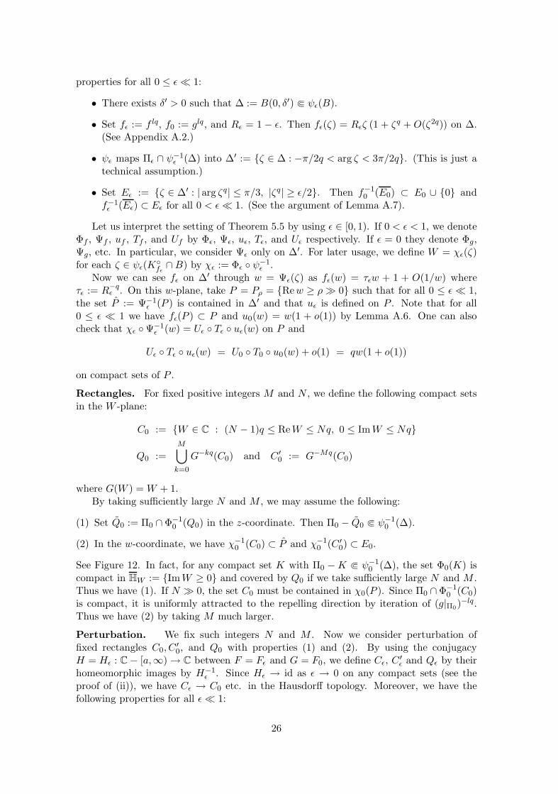
Let us interpret the setting of Theorem 5.5 by using ε ∈ [0, 1). If 0 < ε < 1, we denoteΦf , Ψf , uf , Tf , and Uf by Φε, Ψε, uε, Tε, and Uε respectively. If ε = 0 they denote Φg,Ψg, etc. In particular, we consider Ψε only on Δ′. For later usage, we define W = χε(ζ)for each ζ ∈ ψε(K◦

fε∩B) by χε := Φε ◦ ψ−1

ε .Now we can see fε on Δ′ through w = Ψε(ζ) as fε(w) = τεw + 1 + O(1/w) where

τε := R−qε . On this w-plane, take P = Pρ = {Rew ≥ ρ� 0} such that for all 0 ≤ ε � 1,

the set P := Ψ−1ε (P ) is contained in Δ′ and that uε is defined on P . Note that for all

0 ≤ ε � 1 we have fε(P ) ⊂ P and u0(w) = w(1 + o(1)) by Lemma A.6. One can alsocheck that χε ◦ Ψ−1

ε (w) = Uε ◦ Tε ◦ uε(w) on P and

Uε ◦ Tε ◦ uε(w) = U0 ◦ T0 ◦ u0(w) + o(1) = qw(1 + o(1))

on compact sets of P .

Rectangles. For fixed positive integers M and N , we define the following compact setsin the W -plane:

C0 := {W ∈ C : (N − 1)q ≤ ReW ≤ Nq, 0 ≤ ImW ≤ Nq}

Q0 :=M⋃

k=0

G−kq(C0) and C ′0 := G−Mq(C0)

where G(W ) = W + 1.By taking sufficiently large N and M , we may assume the following:

(1) Set Q0 := Π0 ∩ Φ−10 (Q0) in the z-coordinate. Then Π0 − Q0 � ψ−1

0 (Δ).

(2) In the w-coordinate, we have χ−10 (C0) ⊂ P and χ−1

0 (C ′0) ⊂ E0.

See Figure 12. In fact, for any compact set K with Π0 −K � ψ−10 (Δ), the set Φ0(K) is

compact in HW := {ImW ≥ 0} and covered by Q0 if we take sufficiently large N and M .Thus we have (1). If N � 0, the set C0 must be contained in χ0(P ). Since Π0 ∩Φ−1

0 (C0)is compact, it is uniformly attracted to the repelling direction by iteration of (g|Π0)

−lq.Thus we have (2) by taking M much larger.

Perturbation. We fix such integers N and M . Now we consider perturbation offixed rectangles C0, C

′0, and Q0 with properties (1) and (2). By using the conjugacy

H = Hε : C − [a,∞) → C between F = Fε and G = F0, we define Cε, C ′ε and Qε by their

homeomorphic images by H−1ε . Since Hε → id as ε → 0 on any compact sets (see the

proof of (ii)), we have Cε → C0 etc. in the Hausdorff topology. Moreover, we have thefollowing properties for all ε� 1:

26

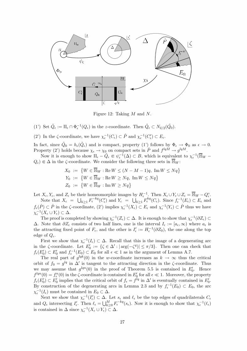
Figure 12: Taking M and N .

(1’) Set Qε := Πε ∩ Φ−1ε (Qε) in the z-coordinate. Then Qε ⊂ Nδ/2(Q0).

(2’) In the ζ-coordinate, we have χ−1ε (Cε) ⊂ P and χ−1

ε (C ′ε) ⊂ Eε.

In fact, since Q0 = hε(Qε) and is compact, property (1’) follows by Φε → Φ0 as ε → 0.Property (2’) holds because χε → χ0 on compact sets in P and f lqM → glqM .

Now it is enough to show Πε − Qε � ψ−1ε (Δ) ⊂ B, which is equivalent to χ−1

ε (HW −Qε) � Δ in the ζ-coordinate. We consider the following three sets in HW :

X0 :={W ∈ HW : ReW ≤ (N −M − 1)q, ImW ≤ Nq

}Y0 :=

{W ∈ HW : ReW ≥ Nq, ImW ≤ Nq

}Z0 :=

{W ∈ HW : ImW ≥ Nq

}Let Xε, Yε, and Zε be their homeomorphic images by H−1

ε . Then Xε ∪Yε∪Zε = HW −Q◦ε .

Note that Xε =⋃

k≥1 F−kqε (C ′

ε) and Yε =⋃

k≥1 Fkqε (Cε). Since f−1

ε (Eε) ⊂ Eε andfε(P ) ⊂ P in the ζ-coordinate, (2’) implies χ−1

ε (Xε) ⊂ Eε and χ−1ε (Yε) ⊂ P thus we have

χ−1ε (Xε ∪ Yε) ⊂ Δ.

The proof is completed by showing χ−1ε (Zε) ⊂ Δ. It is enough to show that χ−1

ε (∂Zε) ⊂Δ. Note that ∂Zε consists of two half lines, one is the interval Iε := [aε,∞) where aε isthe attracting fixed point of Fε, and the other is I ′ε := H−1

ε (∂Z0), the one along the topedge of Qε.

First we show that χ−1ε (Iε) ⊂ Δ. Recall that this is the image of a degenerating arc

in the ζ-coordinate. Let E′0 := {ζ ∈ Δ′ : | arg(−ζq)| ≤ π/3}. Then one can check that

fε(E′0) ⊂ E′

0 and f−1ε (E0) ⊂ E0 for all ε� 1 as in the argument of Lemma A.7.

The real part of glqk(0) in the w-coordinate increases as k → ∞ thus the criticalorbit of f0 = glq in Δ′ is tangent to the attracting direction in the ζ-coordinate. Thuswe may assume that glqn(0) in the proof of Theorem 5.5 is contained in E′

0. Hencef lqn(0) = fn

ε (0) in the ζ-coordinate is contained in E′0 for all ε� 1. Moreover, the property

fε(E′0) ⊂ E′

0 implies that the critical orbit of fε = f lq in Δ′ is eventually contained in E′0.

By construction of the degenerating arcs in Lemma 2.3 and by f−1ε (E0) ⊂ E0, the arc

χ−1ε (Iε) must be contained in E0 ⊂ Δ.

Next we show that χ−1ε (I ′ε) ⊂ Δ. Let sε and �ε be the top edges of quadrilaterals Cε

and Qε intersecting I ′ε. Then �ε =⋃M

k≥0 F−kqε (sε). Now it is enough to show that χ−1

ε (�ε)is contained in Δ since χ−1

ε (Xε ∪ Yε) ⊂ Δ.

27

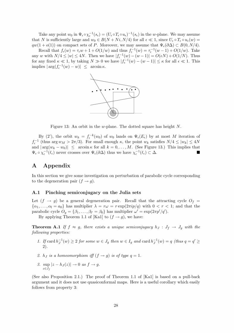
Take any point w0 in Ψε◦χ−1ε (sε) = (Uε◦Tε◦uε)−1(sε) in the w-plane. We may assume

that N is sufficiently large and w0 ∈ B(N +Ni,N/4) for all ε� 1, since Uε ◦Tε ◦uε(w) =qw(1 + o(1)) on compact sets of P . Moreover, we may assume that Ψε(∂Δ) ⊂ B(0, N/4).

Recall that fε(w) = τεw+ 1 +O(1/w) and thus f−1ε (w) = τ−1

ε (w− 1) +O(1/w). Takeany w with N/4 ≤ |w| ≤ 4N . Then we have |f−1

ε (w)− (w− 1)| = O(εN)+O(1/N). Thusfor any fixed κ� 1, by taking N � 0 we have |f−1

ε (w) − (w − 1)| ≤ κ for all ε� 1. Thisimplies | arg(f−1

ε (w) − w)| ≤ arcsinκ.

Figure 13: An orbit in the w-plane. The dotted square has height N .

By (2’), the orbit wk = f−kε (w0) of w0 lands on Ψε(Eε) by at most M iteration of

f−1ε (thus argwM > 2π/3). For small enough κ, the point wk satisfies N/4 ≤ |wk| ≤ 4N

and | arg(wk − w0)| ≤ arcsin κ for all k = 0, . . . ,M . (See Figure 13.) This implies thatΨε ◦ χ−1

ε (�ε) never crosses over Ψε(∂Δ) thus we have χ−1ε (�ε) ⊂ Δ. �

A Appendix

In this section we give some investigation on perturbation of parabolic cycle correspondingto the degeneration pair (f → g).

A.1 Pinching semiconjugacy on the Julia sets

Let (f → g) be a general degeneration pair. Recall that the attracting cycle Of ={α1, . . . , αl = a0} has multiplier λ = rω = r exp(2πip/q) with 0 < r < 1; and that theparabolic cycle Og = {β1, . . . , βl′ = β0} has multiplier ω′ = exp(2πp′/q′).

By applying Theorem 1.1 of [Ka1] to (f → g), we have:

Theorem A.1 If f ≈ g, there exists a unique semiconjugacy hJ : Jf → Jg with thefollowing properties:

1. If cardh−1J (w) ≥ 2 for some w ∈ Jg then w ∈ Ig and cardh−1

J (w) = q (thus q = q′ ≥2).

2. hJ is a homeomorphism iff (f → g) is of type q = 1.

3. supz∈Jf

|z − hJ(z)| → 0 as f → g.

(See also Proposition 2.1.) The proof of Theorem 1.1 of [Ka1] is based on a pull-backargument and it does not use quasiconformal maps. Here is a useful corollary which easilyfollows from property 3:

28

Corollary A.2 As f → g, the Julia set Jf converges to Jg in the Hausdorff topology.

Since hJ ◦ γf and γg determines the same ray equivalence, we have hJ ◦ γf = γg. Forθ ∈ T, put γf (θ) into z in property 3 of the theorem above. Then we have:

Corollary A.3 As f → g, the map γf : T → Jf converges uniformly to γg : T → Jg.

A.2 Normalized form of local perturbation

For a degeneration pair (f → g), the parabolic cycle Og is approximated by an attractingor repelling cycle O′

f with the same period l′ and multiplier λ′ ≈ ω′ = e2πip′/q′ . (SeeSection 2.) Let α′

0 ∈ O′f with α′

0 → β0. Then by looking through the local coordinatesψf (z) = z − α′

0 and ψg(z) = z − β0 near β0 one can view the convergence f l′ → gl′ asfollows:

ψf ◦ f l′ ◦ ψ−1f (z) = λ′z +O(z2)

−→ ψg ◦ gl′ ◦ ψ−1g (z) = ω′z +O(z2).

Here we claim that by replacing ψf → ψg with better local coordinates, we have a nor-malized form of convergence:

ψf ◦ f l′ ◦ ψ−1f (z) = λ′z + zq′+1 +O(z2q′+1)

−→ ψg ◦ gl′ ◦ ψ−1g (z) = ω′z + zq′+1 +O(z2q′+1).

More generally, we have:

Proposition A.4 For ε ∈ [0, 1], let {fε} be a family of holomorphic maps on a neighbor-hood of 0 such that as ε→ 0,

fε(z) = λεz +O(z2) −→ f0(z) = λ0z +O(z2)

where λ0 is a primitive qth root of unity. Then we have a family of holomorphic maps{φε} such that

φε ◦ fε ◦ φ−1ε (z) = λεz + zq+1 +O(z2q+1).

and φε → φ0 near z = 0.

Proof. First suppose that fε(z) = λεz+Aεzn+O(zn+1) where 2 ≤ n ≤ q. Let us consider

a coordinate change by z �→ z − Bεzn with Bε = Aε/(λn+1

ε − λε). Note that λn+1ε − λε is

bounded distance away from 0 when ε� 1, because λε converges to a primitive qth root ofunity. In particular, the coordinate change z �→ z −Bεz

n also converges to z �→ z −B0zn

near 0. By applying these coordinate changes, we can view the family {fε} as

fε(z) = λεz +O(zn+1).

By repeating this process until n = q, we have the family {fε} of the form

fε(z) = λεz + Cεzq+1 +A′

εzn +O(zn+1)

where q + 2 ≤ n ≤ 2q. Next for each ε take a linear coordinate change by z �→ C1/qε z to

normalize Cε to be 1. By taking another coordinate change of the form z �→ ζ = z−B′εz

n

with B′ε = A′

ε/(λn+1ε − λε) again, we have

fε(z) = λεz + zq+1 +O(zn+1).

We can repeat this process until n = 2q and we have the desired form of convergence. �

29

For this new family{fε(z) = λεz + zq+1 +O(z2q+1)

}and n ≥ 0, one can easily check

thatfn

ε (z) = λnε z + Cε,nz

q+1 +O(z2q+1)

where Cε,n is given by the recursive formula Cε,n+1 = λq+1ε Cε,n + λn

ε . Let n = q and setΛε := λq

ε (→ 1 as ε→ 0). By taking linear coordinate changes with z �→ (Cε,q/Λε)1/qz, wehave the convergence of the form

f qε (z) = Λεz (1 + zq +O(z2q))

−→ f q0 (z) = z (1 + zq +O(z2q)).

By further coordinate changes with w = Ψε(z) = −Λqε/(qzq), we have

Ψε ◦ f qε ◦ Ψ−1

ε (w) = Λ−qε w + 1 +O(1/w)

−→ Ψ0 ◦ f q0 ◦ Ψ−1

0 (w) = w + 1 +O(1/w)

on a neighborhood of infinity. Note that we have a similar representation for f l′q′ → gl′q′ .

A.3 Simultaneous linearization

Recently T.Ueda [Ue] showed the simultaneous linearization theorem that explains hyperbolic-to-parabolic degenerations of linearizing coordinates. Here we give a simple version of thetheorem which is enough for our investigation. For R ≥ 0, let ER denote the region{z ∈ C : Re z ≥ R}.

Theorem A.5 (Ueda) For ε ∈ [0, 1], let {fε} be a family of holomorphic maps on{|z| ≥ R > 0} such that

fε(z) = τεz + 1 +O(1/z)−→ f0(z) = z + 1 +O(1/z)

uniformly as ε → 0 where τε = 1 + ε. If R � 0, then for any ε ∈ [0, 1] there exists aholomorphic map uε : ER → C such that

uε(fε(z)) = τεuε(z) + 1

and uε → u0 uniformly on compact sets of ER.

Indeed, Ueda’s original theorem in [Ue] claims that a similar holds for any radialconvergence τε → 1 outside the unit disk. In [Ka4] an alternative proof is given and theerror term O(1/z) is refined to be O(z−1/n) for any n ≥ 1.

Lemma A.6 u0(z) = z(1 + o(1)) as Re z → ∞.

Indeed, it is well-known that if f0(z) = z + 1 + a0/z + · · · then the Fatou coordinate is ofthe form u0(z) = z − a0 log z +O(1). See [Sh] for example.

30

A.4 Small invariant paths joining perturbed periodic points

For a degeneration pair (f → g) in Case (a) (q = q′), we may consider that the paraboliccycle Og is perturbed into the attracting cycle Of with the same period l = l′. (SeeProposition 2.1). In this case, the convergence f lq → glq is viewed as

f lq(z) = rqz + zq +O(z2q) −→ glq(z) = z + zq +O(z2q)

with rq ↗ 1 through suitable local coordinates near β0 ∈ Og as in Appendix A.2.By taking an additional linear coordinate change by z �→ z/r, we consider a family of

holomorphic maps {fε} of the form

fε(z) = λεz(1 + zq +O(z2q))

instead, where we set rq = λε = 1 − ε ↗ 1. Then the local solution of fε(z) = z is z = 0or zq = ε + O(ε2). The latter means q symmetrically arrayed repelling fixed points aregenerated by the perturbation of a parabolic point with multiplicity q+1. Here we claim:

Lemma A.7 For ε � 1, there exist q fε-invariant paths of diameter O(ε1/q) joining thecentral attracting point z = 0 and each of symmetrically arrayed repelling fixed points.

Proof. First we show that D := {z : |z|q ≤ ε/2} satisfies fε(D) ⊂ D◦. By checking thereal part of log fε(z), we have

|fε(z)| = λε|z|(1 + Re zq +O(z2q)).

Since Re zq ≤ ε/2 on D, we have |fε(z)| = |z|(1 − ε/2 +O(ε2)) < |z|.Next we set

E :={z :

ε

2≤ |zq| ≤ 4ε and | arg zq| ≤ π

3

}.

Note that E has q connected components around the repelling fixed points. Now we claimthat E satisfies f−1

ε (E) ⊂ E◦. Since f−1ε is univalent near 0, it is enough to show that

f−1ε (∂E) ⊂ E◦. Set

e1 :={z : |zq| =

ε

2and | arg zq| ≤ π

3

}

e2 :={z : |zq| = 4ε and | arg zq| ≤ π

3

}

e±3 :={z :

ε

2≤ |zq| ≤ 4ε and arg zq = ±π

3

}.

By checking log f−1ε (z), we have

|f−1ε (z)| = λ−1

ε |z|(1 − λ−qε Re zq +O(z2q))

arg f−1ε (z) = arg z − λ−q

ε Im zq +O(z2q).

If z ∈ e1, we have Re zq ≤ ε/2 thus |fε(z)| ≥ |z|(1 + ε/2 + O(ε2)) > |z|. If z ∈ e2, wehave Re zq ≥ 2ε thus |fε(z)| ≤ |z|(1 − ε + O(ε2)) < |z|. For z ∈ e±3 , set |zq| = ρ withε/2 ≤ ρ ≤ 4ε. Then arg f−1

ε (z) = arg z∓ (√

3/2)ρ(1+O(ρ)). Thus we have f−1ε (∂E) ⊂ E◦

in total.Take any q points {z1, · · · , zq} from each connected component of e1. Let ηj be the

segment joining zj and fε(zj). Then the path⋃

k∈Zfk

ε (ηj) has the desired property. �

31

Remark. In Case (b) (q = 1 < q′), the cycle O′f in Appendix A.2 is repelling. By taking

f−l′q′ → g−l′q′ near Og, we have a similar form of the convergence

fε(z) = λεz(1 + zq′ +O(z2q′))

to the case of q = q′, where λε = 1− ε+O(ε2) ∈ C∗. This λε comes from the fact that thenon-zero solutions of fε(z) = z has derivative 0 < r < 1 (Since they are actually pointsin Of in a different coordinate.) One can easily check that the argument of Lemma A.7above also works for this fε and the statement is also true by replacing q with q′.

References

[Cu] G. Cui. Geometrically finite rational maps with given combinatorics. Preprint, 1997.

[DH] A. Douady and J. H. Hubbard. Etude dynamique des polynomes complexes I & II.Pub. Math. Orsay 84–02, 85–05, 1984/85.

[GM] L.R. Goldberg and J. Milnor. Fixed points of polynomial maps, Part II: Fixed pointportraits. Ann. Sci. Ec. Norm. Super. 26(1993), 51–98.

[Ha1] P. Haıssinsky. Modulation dans l’ensemble de Mandelbrot. The Mandelbrot est,Theme and Variations. Tan Lei (ed.), Lond. Math. Soc. Lec. Note Ser. 274, CambridgeUniversity Press, 2000, 37–65.

[Ha2] P. Haıssinsky. Pincement de polynomes. Comment. Math. Helv. 77(2002), 1–23.

[HT] P. Haıssinsky and Tan Lei. Convergence of pinching deformations and matings ofgeometrically finite polynomials. Fund. Math. 181(2004), 143–188.

[Ka1] T. Kawahira. Semiconjugacies between the Julia sets of geometrically finite rationalmaps. Ergodic Theory Dyn. Syst. 23(2003), 1125–1152.

[Ka2] T. Kawahira. Semiconjugacies in complex dynamics with parabolic cycles. Thesis,University of Tokyo, 2003. Available at the Thesis Server in I.M.S. the DynamicalSystems Page:http://www.math.sunysb.edu/dynamics/theses/index.html

[Ka3] T. Kawahira. Tessellation and Lyubich-Minsky laminations associated withquadratic maps II: Topological structures of 3-laminations. Preprint 2006.(arXiv:math.DS/0609836)

[Ka4] T. Kawahira. A proof of simultaneous linearization with a polylog estimate. Toappear in Bull. Polish Acad. Sci. Math. (arXiv:math.DS/0609165)

[Ki] J. Kiwi. Wandering orbit portrait. Trans. Am. Math. Soc. 354(2001) 1437–1485.

[LM] M. Lyubich and Y. Minsky. Laminations in holomorphic dynamics. J. Differ. Geom.47(1997) 17–94.

[Mi1] J. Milnor. Dynamics in one complex variable (3rd edition). Annals of Math Studies160, Princeton University Press, 2006.

32

[Mi2] J. Milnor. Periodic orbits, external rays, and the Mandelbrot set: An expository ac-count. Geometrie complexe et systemes dynamiques., M. Flexor (ed.) et al. Asterisque261(2000), 277-333.

[Po] Ch. Pommerenke. Boundary behaviour of conformal maps. Springer-Verlag, 1992.

[Sh] M. Shishikura. The Hausdorff dimension of the boundary of the Mandelbrot set andJulia sets. Ann. of Math. 147(1998), 225–267.

[T] Tan Lei. On pinching deformation of rational maps. Ann. Sci. Ec. Norm. Super.35(2002), 353–370.

[Ue] T. Ueda. Schroder equation and Abel equation. Manuscript.

33