Tesfamariam, S., & Goda, K. (2015). Loss estimation for non-ductilereinforced concrete building in Victoria, British Columbia, Canada:effects of mega-thrust Mw9-class subduction earthquakes andaftershocks. Earthquake Engineering and Structural Dynamics,44(13), 2303-2320. https://doi.org/10.1002/eqe.2585

Peer reviewed version

Link to published version (if available):10.1002/eqe.2585

Link to publication record in Explore Bristol ResearchPDF-document

This is the peer reviewed version of the following article: Tesfamariam, S., and Goda, K. (2015) Loss estimationfor non-ductile reinforced concrete building in Victoria, British Columbia, Canada: effects of mega-thrust Mw9-class subduction earthquakes and aftershocks. Earthquake Engng Struct. Dyn., 44: 2303–2320, which has beenpublished in final form at http://dx.doi.org/10.1002/eqe.2585. This article may be used for non-commercialpurposes in accordance with Wiley Terms and Conditions for Self-Archiving.

University of Bristol - Explore Bristol ResearchGeneral rights

This document is made available in accordance with publisher policies. Please cite only thepublished version using the reference above. Full terms of use are available:http://www.bristol.ac.uk/red/research-policy/pure/user-guides/ebr-terms/

Loss estimation for non-ductile reinforced concrete building in Victoria, British Columbia, Canada: Effects of mega-thrust Mw9-class

subduction earthquakes and aftershocks

Solomon Tesfamariam1,,†1 and Katsuichiro Goda2

1School of Engineering, The University of British Columbia, Kelowna, British Columbia, Canada V1V 1V7 2Department of Civil Engineering, University of Bristol, University Walk, Bristol, United Kingdom BS8 1TR

SUMMARY

This paper presents, within the performance-based earthquake engineering framework, a comprehensive probabilistic seismic loss estimation method that accounts for main sources of uncertainty related to hazard, vulnerability, and loss. The loss assessment rigorously integrates multiple engineering demand parameters (maximum and residual inter-story drift ratio, and peak floor acceleration) with consideration of mainshock-aftershock sequences. A 4-story non-ductile reinforced concrete building located in Victoria, British Colombia, Canada is considered as a case study. For 100 mainshock and mainshock-aftershock earthquake records, incremental dynamic analysis is performed, and the three engineering demand parameters are fitted with a probability distribution and corresponding dependence computed. Finally, with consideration of different demolition limit states, loss assessment is performed. From the results, it can be shown that when seismic vulnerability models are integrated with seismic hazard, the aftershock effects are relatively minor in terms of overall seismic loss (1-4% increase). Moreover, demolition limit state parameters, uncertainties of collapse fragility and non-collapse seismic demand prediction models have showed significant contribution to the loss assessment. The seismic loss curves for the reference case and for cases with the varied parameters can differ by as large as about 150%.

KEY WORDS: Peak inter-story drift, Residual inter-story drift, Non-ductile reinforced concrete frame, Loss assessment

1. INTRODUCTION

Victoria is the capital city of British Columbia (BC), Canada, on Vancouver Island, facing the Strait of Juan de Fuca. Three earthquake types, namely shallow crustal earthquakes, deep inslab earthquakes, and mega-thrust Cascadia subduction earthquakes, contribute significantly to overall seismic hazard [1,2]. Since 1900, several destructive earthquakes have occurred: 1918 and 1946 earthquakes in Vancouver Island and 1949, 1965, and 2001 (Nisqually) deep earthquakes in Washington, USA. Moreover, paleoseismic data, such as onshore tsunami deposits and submarine turbidite deposits [3], indicate that mega-thrust earthquakes had occurred repeatedly in the Cascadia subduction zone, involving the oceanic

1*Correspondence to: Solomon Tesfamariam, School of Engineering, The University of British Columbia, 3333 University Way, Kelowna, British Columbia, Canada V1V 1V7 †E-mail: solomon.tesfamariam@ubc.ca

2

Juan de Fuca, Gorda, and Explorer plates moving against the continental North American plate. Because of different source and path characteristics of these earthquakes, amplitude, duration, and frequency content of typical ground motions for the three types differ. A previous regional seismic risk assessment exercise carried out by Onur et al. [4] indicated that seismic risk to vulnerable parts of older constructions in Victoria is high. In addition, a recent study by AIR Worldwide [5] suggested that regional economic loss associated with a hypothetical Mw9 Cascadia earthquake scenario can be significant.

An accurate assessment of potential impact of future destructive earthquakes is essential for effective disaster risk reduction and requires decision-support tools that facilitate the quantitative seismic loss estimation. Probabilistic seismic risk analysis (PSRA) entails comprehensive understanding of ground shaking information, such as fault rupture process, wave propagation, and site effects, as well as vulnerability of structures, such as structural damage accumulation, seismic loss generation, and societal/economic impact [6-8]. Through probabilistic calculus, PSRA evaluates the potential damage and loss that a certain group of structures is likely to experience due to various seismic events.

A seismic demand model characterizes a probabilistic relationship between seismic intensity measure (IM) and engineering demand parameter (EDP). For such purposes, incremental dynamic analysis (IDA) has been adopted widely [9]. In IDA, a series of nonlinear dynamic analyses are conducted by scaling a set of input ground motions based on an adopted IM, and prediction equations of EDP at different IM levels are developed. Luco and Bazzurro [10] indicated that excessive record scaling can induce bias in the estimated seismic demand and that ensuring the similarity of the response spectral shape of the selected records with a target response spectrum is a crucial factor. To avoid significant bias in assessing seismic performance of a structure, Baker [11] proposed a record selection method using conditional mean spectra (CMS) as target, rather than uniform hazard spectrum (UHS) as specified in building codes, by taking into account inter-period correlation of response spectral ordinates at different vibration periods. Furthermore, Goda and Atkinson [12] extended the CMS-based record selection approach by defining multiple target CMS for different earthquake types in subduction zones.

EDP is either uni-variate or multi-variate. When a scalar parameter that correlates well with damage severity (e.g. inter-story drift ratio, ISDR) is adopted, detailed probabilistic models are developed using seismic demand estimation methods for structures of interest. The multi-variate case is often implemented using fragility models for different types of damage sensitivity (e.g. drift-sensitive versus acceleration-sensitive). However, the fragility curves for different EDP parameters are often evaluated separately, and thus dependence of the EDP for a given IM is not taken into account explicitly. Recently, Ruiz-Garcia and Miranda [13] and Ramirez and Miranda [14] have included residual drift as EDP, in addition to maximum ISDR and peak floor acceleration (PFA). Performance matrices based on both maximum and residual drifts have been recently proposed [15,16]. In the above-mentioned approaches, assessment of maximum and residual drift ratios, which are physically inter-related and thus statistically correlated, has not been elaborated. Therefore, rigorous evaluation of joint probability distributions of the maximum and residual drift ratios for realistic multi-degree-of-freedom (MDOF) systems is necessary.

Incorporating aftershock ground motions into conventional PSRA, which mainly concerns mainshock ground motions, is a timely research topic [17-20]. As repairs of mainshock-damaged buildings are not usually completed during an ongoing aftershock

3

sequence (up to a few months after a mainshock), large aftershocks potentially increase the damage severity of mainshock-damaged buildings and cause additional damage and loss.

The main objective of this study is to develop a comprehensive PSRA framework that rigorously integrates multiple EDPs (maximum and residual ISDR and PFA) with consideration of mainshock-aftershock (MSAS) earthquake sequences. The innovative features of the developed PSRA tool are: (1) the incorporation of strong-motion mainshock records as well as MSAS sequence records from the 2011 Mw9 Tohoku, Japan earthquake, which is the best available proxy to a future Cascadia subduction event (Sections 2.2 and 2.3); (2) updating of IDA-based seismic vulnerability models using the extensive set of input records that are carefully selected by reflecting regional seismic hazard (Sections 2.3 and 2.4); and (3) extension of the conventional uni-variate seismic fragility models into copula-based multi-variate models (Section 2.5), facilitating the consideration of multiple seismic loss generation mechanisms (i.e. non-collapse damage, collapse, and demolition). The developed framework is applied to a 4-story non-ductile reinforced concrete (RC) building located in Victoria, BC as a case study. This type of structures is more susceptible to seismic damage in comparison with modern code-conforming RC buildings [21,22]. The building used in this study was modeled by Liel and Deierlein [23] and designed according to the provisions of the 1967 Uniform Building Code (UBC) [24]. Albeit with some modifications, the Canadian design code adopted in the 1960’s followed the UBC [25]. For the seismicity of Victoria, BC, mega-thrust Mw9-class subduction earthquakes and aftershocks are considered.

2. FRAMEWORK FOR SEISMIC LOSS MODEL

The major consideration in modeling seismic loss is the proper treatment of uncertainties in the quantification of demand and capacity, and cost incurred due to unsatisfactory performance. The uncertainty in demand, capacity, and ensuing damage can be quantified probabilistically through inelastic seismic demand prediction models, seismic fragility models, and damage-loss functions. For this purpose, the performance-based earthquake engineering (PBEE) methodology can be employed to assess seismic vulnerability of facilities and components that contribute to specified levels of consequences [7-9]. Typically, an analytical procedure of PBEE consists of seismic hazard analysis, structural analysis, damage analysis, and loss analysis. A computational flow of the PBEE is illustrated in Figure 1.

In the PBEE-based seismic loss estimation method, hazard analysis evaluates ground motion intensity measures (IM) based on seismological and geotechnical data. Typically, hazard analysis is conducted to express seismic hazard in terms of mean annual probability of exceedance, p[IM], which is specific to the location and design characteristics of a facility. The second step is structural analysis in which an appropriate structural model is used to calculate EDP and to estimate collapse capacity/probability. The structural behavior can be characterized in terms of displacement, force, and other quantities. To assess the probability of attaining a specific structural response level, conditioned on seismic excitation p[EDP|IM], various methods are used. Subsequently, damage analysis relates the EDP to damage measures (DM), which describe physical extent of structural damage. The output of damage analysis is a fragility function that estimates the probability of attaining various damage levels conditioned on structural response, p[DM|EDP]. Finally, loss analysis evaluates seismic performance, parameterized with different decision variables (DV), conditioned on damage, p[DV|DM]. DV is often taken to represent repair and reconstruction costs, downtime (loss of operability), and casualties.

4

Figure 1. Probabilistic seismic risk analysis procedure.

2.1 Building model

The 4-story office building (Figure 2a), with an RC space frame lateral resisting system (ID 3004 in Liel and Deierlein [23]), has a floor plan measuring 125 ft by 175 ft and columns spaced at 25 ft. The total height of the structure is 54 ft, with ground and higher floor levels story heights being 15 ft and 13 ft, respectively. The 1967 UBC seismic provisions are applied. The structure is designed as a space frame, such that all columns and beams are part of the lateral resisting system, and with concrete strength f’c = 27.6 MPa and reinforcing bars with fy = 413.7 MPa in both beams and columns. All beam and column elements have the same amount of over-strength, such that each element is 15% stronger than the code-

5

minimum design level. The design is governed by strength and stiffness requirements, as the 1967 UBC had few requirements for special seismic design or ductile detailing.

The non-ductile structure is modeled in OpenSees following a lumped plasticity approach (see Liel and Deierlein [23] for details). The lumped plasticity element models used to simulate plastic hinges in beam-column elements (Figure 2b) adopt a nonlinear spring model developed by Ibarra et al. [26]. This model is capable of capturing important modes of deterioration that lead to side-sway collapse of RC frames. Modal analysis of the finite-element model indicates that the first three modal periods of the 4-story frame are 1.92, 0.55, and 0.27 s, respectively. The first vibration period of the structural model is relatively long for a typical 4-story building. The reasons for this are attributed to [23]: (i) neglected stiffness contributions from non-structural components and structural components that are not part of the lateral resisting system; (ii) additional flexibility resulting from the use of the secant stiffness to model RC elements; and (iii) consideration of bond-slip deformations in RC elements.

Figure 2. Nonlinear finite-element model (a) and backbone curve for beam-column elements (b) of 4-story non-ductile RC frame. The figure is modified after [23].

2.2 Seismic hazard and input ground motion selection

The case study site is focused upon Victoria, where non-seismically designed vulnerable RC frames exist and are still in use. There are mainly three potential sources of damaging earthquakes: shallow crustal earthquakes, off-shore mega-thrust interface earthquakes from the Cascadia subduction zone, and deep inslab earthquakes [1]. The expected moment magnitude of the Cascadia subduction events is in the range of 8 to 9, and its mean recurrence period ranges from 500 to 600 years (note: the last event occurred in 1700). Atkinson and Goda [2] carried out the regional seismic hazard assessment by taking into account: (1) use of a longer earthquake catalog based on a uniform moment magnitude scale in developing revised magnitude-recurrence relationships for seismic source zones; (2) use of newer ground motion prediction equations with proper distance measure conversion by accounting for finite fault plane size; (3) logic-tree representation of alternative equations to account for epistemic uncertainty in ground motion prediction; and (4) probabilistic scenarios for the potential mega-thrust Cascadia earthquakes. The seismic hazard modeling is implemented using Monte Carlo simulation and thus can generate a synthetic earthquake

6

catalog, containing information on occurrence time, location and magnitude of an earthquake, geometry of fault rupture, and predicted ground motion parameters (i.e. IM). A full range of uncertainties, as implemented in probabilistic seismic hazard analysis (PSHA), is considered in the assessment. The values of IM are then employed to estimate EDP using inelastic seismic demand prediction models.

Figure 3 shows UHS and seismic deaggregation for Victoria (site class C) at the return period of 2500 years. The vibration period for seismic deaggregation is 2.0s (i.e. spectral period for IM). It is important to recognize that the UHS ordinates are computed based on numerous earthquake scenarios that may occur in a seismic region of interest, and dominant scenarios at different spectral periods are not identical, as source, path, and site characteristics affect frequency content of ground motions differently. In deaggregation plot, dominant scenarios are represented in terms of magnitude, distance, and earthquake type (crustal/interface/inslab). Different earthquake types are associated with distinct event features in terms of magnitude and distance. For instance, the magnitude and distance of the Cascadia subduction events range between 8 and 9 and between 50 and 100 km, respectively, which are constrained by physical characteristics of the Cascadia scenarios. At the return period of 2500 years, 50% of the dominant scenarios are originated from the mega-thrust subduction zone. This is an important consideration for seismic performance evaluation of (relatively flexible) structures in south-western BC.

Figure 3. Comparison of UHS and CMS (a) and seismic deaggregation (b) for Victoria (site class C) at return period of 2500 years.

The ground motion input should reflect regional seismic hazard characteristics in south-western BC. To include suitable ground motion records for the mega-thrust Cascadia subduction events, a new database for real MSAS records has been compiled by incorporating the 2011 Mw9 Tohoku earthquake records. The database combines recordings from the PEER-NGA database and from the three national/regional networks in Japan (i.e. K-NET/KiK-net and SK-net). The Tohoku dataset is particularly relevant to the Cascadia subduction event, because of anticipated macro-level similarity between these two mega-thrust subduction events, which is not present in ground motion data from other smaller earthquakes.

7

The database consists of 606 MSAS sequences; 75 sequences from the PEER-NGA database (same sequences used by Goda and Taylor [27]) and 531 sequences from the Japanese databases. All records (i.e. both mainshocks and aftershocks) satisfy the following criteria: (i) moment magnitude is greater than or equal to 5.0 (note: minimum magnitude for mainshocks is set to 5.9), (ii) focal depth is less than 150 km, (iii) average shear-wave velocity in the top 30 m is between 50 and 2500 m/s (note: majority of records are for site classes C and D), (iv) source-to-site distance is less than 300 km (as a function of moment magnitude), and (v) average peak ground acceleration (PGA) of the two horizontal components is greater than 75 cm/s2. The MSAS sequences are constructed by applying time-space windows (typically, 100 days before and after a reference event and space window is defined in terms of magnitude of the reference event) and by limiting the difference of focal depths within 30 km. The search process is iterative and continued until all candidate events are identified and included in the MSAS database. In each sequence, an event with the largest magnitude and the second largest magnitude is designated as mainshock and major aftershock, respectively. The magnitudes of mainshocks are greater by approximately one magnitude unit than those of major aftershocks. An implication of the differences is that spectral content of mainshock records and aftershock records differ significantly (on average), which is important when record scaling is implemented in IDA [28].

2.3 Response spectra matching to target conditional mean spectra

For south-western BC, where seismic events having distinct response spectral features contribute significantly to overall seismic hazard (Figure 3b), a multiple-conditional mean spectra (CMS)-based method should be considered by defining target CMS for each of the major earthquake sources [12]. Figure 3a compares UHS and CMS for three earthquake event types for Victoria at the return period of 2500 years. The anchor vibration period in developing CMS is 2 s, which is close to the fundamental vibration period of the frame (i.e. 1.92 s). The CMS are usually lower than the corresponding UHS. The response spectral shape for crustal events has more spectral content in the short vibration period range in comparison with that for interface events, reflecting complicated interactions of dominant earthquake scenarios and ground motion models used in PSHA for different earthquakes.

Using the new database for MSAS sequences and the constructed CMS, record selection is carried out. The matching of individual response spectra with target CMS is implemented for mainshock records within individual sequences, consistent with how CMS are constructed (i.e. aftershock effects are not included in PSHA). For the return period of 2500 years, 50 records (2 horizontal components for each record) are chosen such that response spectra of these records match the target CMS closely in a least squares sense. The matching of the target and candidate response spectra is performed based on the geometric mean of two horizontal components for the vibration period range between 0.3 and 3.0 s. This range includes both longer and shorter sides of vibration periods with respect to the anchor vibration period (i.e. 2 s). The match in the longer side of the vibration period range is important, when a structure undergoes large displacement and its vibration period becomes longer. On the other hand, the match in the shorter side of the vibration period range can be important when high vibration modes are excited by input ground motions. In particular, for the 4-story non-ductile RC frame, the considered vibration period range covers the main vibration periods of interest. The number of records for each earthquake type (crustal/interface/inslab), out of 50 records, is determined based on its relative contribution to seismic hazard using seismic deaggregation results. At the return period level of 2500 years, the number of records for crustal, interface, and inslab events is 13, 25, and 12, respectively.

8

2.4 Seismic demand modeling

To incorporate the aftershock effects in the assessment, seismic demand models of the 4-story non-ductile RC frame, are developed using MSAS sequences as seismic input [19,20]. Moreover, damage-loss models involve multiple EDP variables because different building components are sensitive to different types of seismic effects (e.g. acceleration-sensitive versus drift-sensitive). Typical EDP parameters include the maximum ISDR and PFA for structural and non-structural components [14,29]. In addition to the transient EDP parameters, residual ISDR may be a critical parameter in determining the usability of damaged structures in a post-earthquake situation [14,16]. Therefore, the EDP considered in this study includes the maximum ISDR (MaxISDR), residual ISDR (ResISDR), and peak floor acceleration (PFA). The above situation requires the joint probabilistic modeling of multi-variate EDP. This study addresses this problem by adopting multi-variate seismic demand models for which detailed characterizations of marginal probability distributions for MaxISDR, ResISDR, and PFA (at various IM levels) and dependence (copula) models between MaxISDR and ResISDR are carried out and reported in Goda and Tesfamariam [30].

2.5 Damage-loss modeling

The damage-loss analysis is conducted by using a so-called story-based loss estimation following Ramirez and Miranda [14], where for each EDP corresponding damage/loss at story level is computed. The formulation of the story-based seismic loss estimation simplifies a process of calculating seismic loss (i.e. DV) as a function of EDP, rather than DM, and it requires less information on structural details and their costs. The seismic loss LT for given EDP can be expressed as [14]:

CDNCT LLLL (1)

where LNC, LD, and LC are the seismic losses for non-collapse repairs (NC), demolition (D), and collapse (C) cases, respectively. The three situations are disjoint and mutually exclusive. The numerical evaluation of LT in PSRA calculations is facilitated as follows: (i) collapse probability is assessed for the EDP; if collapse is predicted, then LT = LC; (ii) demolition is considered for non-collapsed structure and it is determined according to a realized value of ResISDR (contained in EDP) in comparison with the (uncertain) limit state function for demolition; if demolition is predicted, then LT = LD; and (iii) otherwise, LNC is assessed by using EDP-DV functions for non-collapse cases. It is noted that LNC, LD, and LC are random variables. Ramirez and Miranda [14] adopted the limit state function for demolition representing a lognormal fragility curve (i.e. G(D|ResISDR) = 1-(log(ResISDR/D)/D), where is the standard normal distribution function, and D and D are the median and logarithmic standard deviation of the demolition fragility curve, respectively).

The procedure for developing the EDP-DV functions for the 4-story non-ductile RC frame follows the method suggested by Ramirez and Miranda [14]. First, component fragility groups (i.e. damage sensitivity) and story-based cost distributions are assigned to major building components. The expected (normalized) loss in component j conditioned on non-collapse (NC) and EDP, E[Lj|NC,EDPj] is a function of the component’s repair cost when it is in a different damage state and the probability of being in each damage state:

m

ijiijjj EDPNCdsDSpDSNCLEEDPNCLE

1

,|,|,| (2)

where m is the number of damage states for component j, E[Lj|NC,DSi] is the expected value of the normalized loss for component j when it is in a damage state i, DSi, and

9

p(DS=dsi|NC,EDPj) is the probability of the jth component being in a damage state i, dsi, given that it is subjected to a demand of EDPj. The probability of being in each damage state for component j can be obtained from component-specific fragility functions. The EDP-DV functions are developed based subcontractor category (e.g. concrete, finish, and mechanical), in addition to story as well as damage sensitivity. The main reason for such development is to take into account uncertainties of damage-loss functions adequately, noting that probability distribution type (i.e. lognormal distribution) and variability (i.e. coefficient of variation) for the EDP-DV functions are available for subcontractor basis only. Figure 4 shows mean EDP-DV functions for 9 subcontractor-sensitivity combinations at ground floor (normalized by story-level loss). The corresponding coefficients of variation are indicated inside the parentheses of the figure legend.

Figure 4. EDP-DV functions for 9 subcontractor-sensitivity combinations (ground floor). The coefficient of variation for each EDP-DV function is included in the parentheses.

3. RESULTS AND DISCUSSION

IDA is carried out for the 4-story non-ductile RC frame using a set of 50 MSAS sequences (i.e. 100 horizontal components) as well as a set of 50 MS records (to evaluate the effect of aftershocks). The seismic intensity level (i.e. IM) is specified in terms of spectral acceleration at 2 s and ranges from 0.05 to 0.7 g (in total, 30 levels). For each nonlinear dynamic analysis, MaxISDR, ResISDR, and PFA at all four story levels for individual record segments are stored for post-processing. In general, numerical instability is encountered when the ISDR of the frame exceeds 0.10. The occurrence of such large-deformation responses for the first time is treated as ‘collapse’ in this study. This definition of collapse capacity is consistent with Vamvatsikos and Cornell [9]. Two out of 50 sequences have major foreshocks prior to mainshocks; in these cases, the nonlinear responses due to MSAS sequences can be less than those due to MS records only (depending on the IM level).

In Figure 5, time-history responses (floor acceleration and inter-story drift ratio) of the 4-story non-ductile RC frame subjected to a MSAS sequence (input accelerogram is scaled to a seismic intensity level of 0.2 g) are depicted. The mainshock is for Mw = 9.1 recorded at a distance of 109 km, whereas the aftershock is for Mw = 7.1 recorded at a distance of 59 km. From the figure, it can be shown that the maximum ISDR at the ground floor is higher, and

10

decreases with increase in the story level. There is an appreciable residual ISDR. On the other hand, the difference in the acceleration at all story levels is minimal (more on this will be discussed in the subsequent section).

Figure 5. Time-history responses (floor acceleration and inter-story drift ratio) of the 4-story non-ductile RC frame subjected to a MSAS sequence (input accelerogram is scaled to a

seismic intensity level of 0.2 g).

3.1 Incremental dynamic analysis

The main IDA results for both MS records and MSAS sequences are shown in Figure 6. To present the uncertainty of the IDA results succinctly, two sets of percentile curves, i.e. 16th-84th curves and 2.5th-97.5th curves, are included in the figure. The two sets approximately correspond to mean plus/minus one standard deviation and mean plus/minus two standard deviations. The results shown in Figure 6 suggest that the overall characteristics of the IDA curves for MaxISDR and ResISDR are different; the former increases gradually with the seismic intensity level, while the latter increases rapidly when the seismic intensity level reaches about 0.15 g (at which the corresponding median MaxISDR is about 0.025). It is noteworthy that the uncertainty of ResISDR is much greater than that of MaxISDR. The IDA results for PFA show linear trends. Looking at the EDP-DV functions for the non-ductile RC frame (Figure 4), impact due to acceleration may be less significant in comparison with that due to drift.

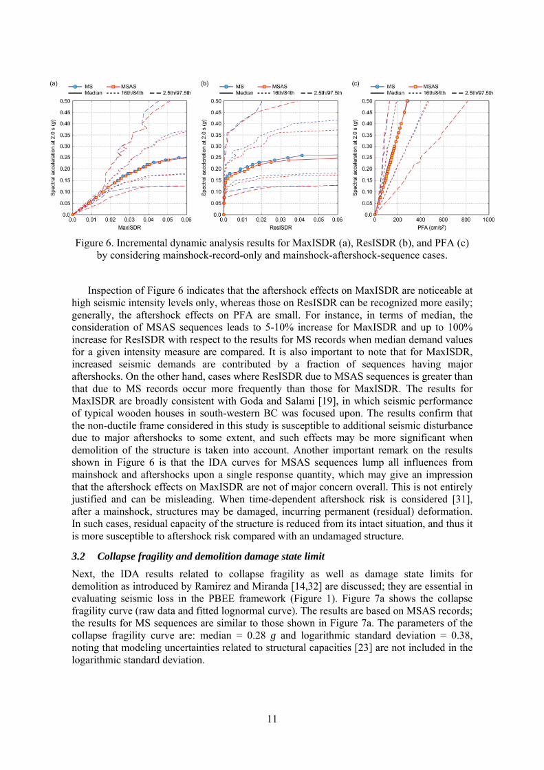
11

Figure 6. Incremental dynamic analysis results for MaxISDR (a), ResISDR (b), and PFA (c) by considering mainshock-record-only and mainshock-aftershock-sequence cases.

Inspection of Figure 6 indicates that the aftershock effects on MaxISDR are noticeable at high seismic intensity levels only, whereas those on ResISDR can be recognized more easily; generally, the aftershock effects on PFA are small. For instance, in terms of median, the consideration of MSAS sequences leads to 5-10% increase for MaxISDR and up to 100% increase for ResISDR with respect to the results for MS records when median demand values for a given intensity measure are compared. It is also important to note that for MaxISDR, increased seismic demands are contributed by a fraction of sequences having major aftershocks. On the other hand, cases where ResISDR due to MSAS sequences is greater than that due to MS records occur more frequently than those for MaxISDR. The results for MaxISDR are broadly consistent with Goda and Salami [19], in which seismic performance of typical wooden houses in south-western BC was focused upon. The results confirm that the non-ductile frame considered in this study is susceptible to additional seismic disturbance due to major aftershocks to some extent, and such effects may be more significant when demolition of the structure is taken into account. Another important remark on the results shown in Figure 6 is that the IDA curves for MSAS sequences lump all influences from mainshock and aftershocks upon a single response quantity, which may give an impression that the aftershock effects on MaxISDR are not of major concern overall. This is not entirely justified and can be misleading. When time-dependent aftershock risk is considered [31], after a mainshock, structures may be damaged, incurring permanent (residual) deformation. In such cases, residual capacity of the structure is reduced from its intact situation, and thus it is more susceptible to aftershock risk compared with an undamaged structure.

3.2 Collapse fragility and demolition damage state limit

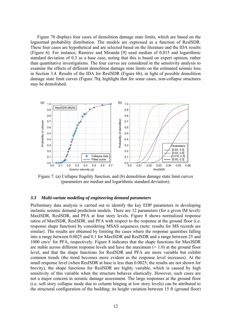
Next, the IDA results related to collapse fragility as well as damage state limits for demolition as introduced by Ramirez and Miranda [14,32] are discussed; they are essential in evaluating seismic loss in the PBEE framework (Figure 1). Figure 7a shows the collapse fragility curve (raw data and fitted lognormal curve). The results are based on MSAS records; the results for MS sequences are similar to those shown in Figure 7a. The parameters of the collapse fragility curve are: median = 0.28 g and logarithmic standard deviation = 0.38, noting that modeling uncertainties related to structural capacities [23] are not included in the logarithmic standard deviation.

12

Figure 7b displays four cases of demolition damage state limits, which are based on the lognormal probability distribution. The models are expressed as a function of ResISDR. These four cases are hypothetical and are selected based on the literature and the IDA results (Figure 6). For instance, Ramirez and Miranda [9] used median of 0.015 and logarithmic standard deviation of 0.3 as a base case, noting that this is based on expert opinion, rather than quantitative investigations. The four curves are considered in the sensitivity analysis to examine the effects of different demolition damage state limits on the estimated seismic loss in Section 3.4. Results of the IDA for ResISDR (Figure 6b), in light of possible demolition damage state limit curves (Figure 7b), highlight that for some cases, non-collapse structures may be demolished.

Figure 7. (a) Collapse fragility function, and (b) demolition damage state limit curves (parameters are median and logarithmic standard deviation).

3.3 Multi-variate modeling of engineering demand parameters

Preliminary data analysis is carried out to identify the key EDP parameters in developing inelastic seismic demand prediction models. There are 12 parameters (for a given IM level): MaxISDR, ResISDR, and PFA at four story levels. Figure 8 shows normalized response ratios of MaxISDR, ResISDR, and PFA with respect to the response at the ground floor (i.e. response shape function) by considering MSAS sequences (note: results for MS records are similar). The results are obtained by limiting the cases where the response quantities falling into a range between 0.0025 and 0.1 for MaxISDR and ResISDR and a range between 25 and 1000 cm/s2 for PFA, respectively. Figure 8 indicates that the shape functions for MaxISDR are stable across different response levels and have the maximum (= 1.0) at the ground floor level, and that the shape functions for ResISDR and PFA are more variable but exhibit common trends (the trend becomes more evident as the response level increases). At the small response level (when ResISDR at base is less than 0.0025; the results are not shown for brevity), the shape functions for ResISDR are highly variable, which is caused by high sensitivity of this variable when the structure behaves elastically. However, such cases are not a major concern in seismic damage assessment. The large responses at the ground floor (i.e. soft story collapse mode due to column hinging at low story levels) can be attributed to the structural configuration of the building; its height variation between 15 ft (ground floor)

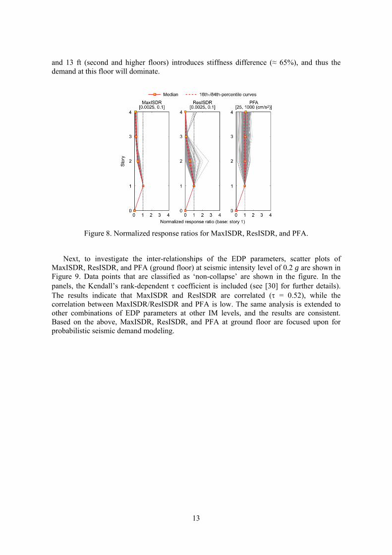
13

and 13 ft (second and higher floors) introduces stiffness difference (≈ 65%), and thus the demand at this floor will dominate.

Figure 8. Normalized response ratios for MaxISDR, ResISDR, and PFA.

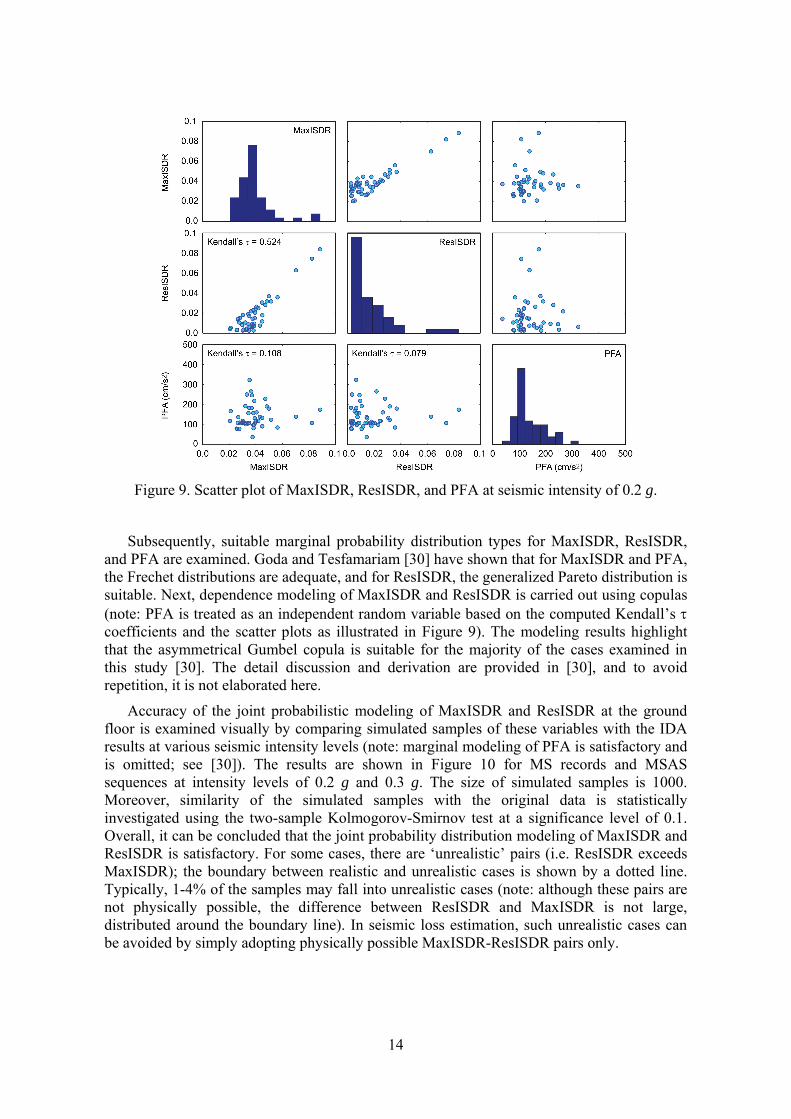
Next, to investigate the inter-relationships of the EDP parameters, scatter plots of MaxISDR, ResISDR, and PFA (ground floor) at seismic intensity level of 0.2 g are shown in Figure 9. Data points that are classified as ‘non-collapse’ are shown in the figure. In the panels, the Kendall’s rank-dependent coefficient is included (see [30] for further details). The results indicate that MaxISDR and ResISDR are correlated ( = 0.52), while the correlation between MaxISDR/ResISDR and PFA is low. The same analysis is extended to other combinations of EDP parameters at other IM levels, and the results are consistent. Based on the above, MaxISDR, ResISDR, and PFA at ground floor are focused upon for probabilistic seismic demand modeling.

14

Figure 9. Scatter plot of MaxISDR, ResISDR, and PFA at seismic intensity of 0.2 g.

Subsequently, suitable marginal probability distribution types for MaxISDR, ResISDR, and PFA are examined. Goda and Tesfamariam [30] have shown that for MaxISDR and PFA, the Frechet distributions are adequate, and for ResISDR, the generalized Pareto distribution is suitable. Next, dependence modeling of MaxISDR and ResISDR is carried out using copulas (note: PFA is treated as an independent random variable based on the computed Kendall’s coefficients and the scatter plots as illustrated in Figure 9). The modeling results highlight that the asymmetrical Gumbel copula is suitable for the majority of the cases examined in this study [30]. The detail discussion and derivation are provided in [30], and to avoid repetition, it is not elaborated here.

Accuracy of the joint probabilistic modeling of MaxISDR and ResISDR at the ground floor is examined visually by comparing simulated samples of these variables with the IDA results at various seismic intensity levels (note: marginal modeling of PFA is satisfactory and is omitted; see [30]). The results are shown in Figure 10 for MS records and MSAS sequences at intensity levels of 0.2 g and 0.3 g. The size of simulated samples is 1000. Moreover, similarity of the simulated samples with the original data is statistically investigated using the two-sample Kolmogorov-Smirnov test at a significance level of 0.1. Overall, it can be concluded that the joint probability distribution modeling of MaxISDR and ResISDR is satisfactory. For some cases, there are ‘unrealistic’ pairs (i.e. ResISDR exceeds MaxISDR); the boundary between realistic and unrealistic cases is shown by a dotted line. Typically, 1-4% of the samples may fall into unrealistic cases (note: although these pairs are not physically possible, the difference between ResISDR and MaxISDR is not large, distributed around the boundary line). In seismic loss estimation, such unrealistic cases can be avoided by simply adopting physically possible MaxISDR-ResISDR pairs only.

15

Figure 10. Comparison of scatter plots of MaxISDR and ResISDR based on the IDA results and simulated samples at seismic intensity levels of 0.2 g (a) and 0.3 g (b).

Finally, to evaluate the relative contributions of different types of seismic failure modes (i.e. collapse, demolition, and non-collapse damage), the mean IM-DV functions are developed by generating 10,000 samples of seismic damage costs for each IM level. Figure 11 shows the results for two sets of parameters for the demolition damage limit state (i.e. median and logarithmic standard deviation): [0.015, 0.3] and [0.03, 0.3] (Figure 7b). In each figure, four IM-DV functions for collapse, demolition, non-collapse damage, and total damage are included for MS records and MSAS sequences. The key observations from Figure 11 are:

i. The collapse IM-DV curves for MS records and MSAS sequences are almost identical.

ii. The differences between MS records and MSAS sequences for the non-collapse IM-DV curves are small. MSAS sequences result in greater seismic loss for the IM levels less than 0.2 g; the seismic loss for MSAS sequences becomes less than that for MS records for the IM levels greater than 0.2 g, because the demolition failure mode becomes more dominant at higher IM levels (given no collapse).

iii. The effects of aftershocks on seismic loss are most noticeable on the demolition failure mode. This is caused by the increased residual seismic demand due to major aftershocks (Figure 6).

iv. The effects due to aftershocks on seismic loss are sensitive to the adopted demolition damage state limits. When the median limit state for demolition is small (Figure 11a), the demolition failure mode consists of about 30% of the entire failures (peaked at around IM equal to 0.22 g). When the median is larger (Figure 11b), the frequency of the demolition becomes smaller and the collapse failure mode becomes more dominant.

16

Figure 11. Comparison of IM-DV functions for collapse, demolition, non-collapse damage, and total cost by considering two sets of demolition damage state limit parameters: (a)

[0.015, 0.3] and (b) [0.03, 0.3].

3.4 Seismic loss estimation

To investigate the key issues related to the developed seismic loss estimation tool and to investigate the effects of aftershocks on the estimated seismic loss, twelve analysis cases are set up (Table 1). The common setting for all twelve cases is: the marginal probability distribution types for MaxISDR, ResISDR, and PFA are the Frechet, generalized Pareto, and Frechet models, respectively; the dependence (copula) function for MaxISDR and ResISDR is the asymmetrical Gumbel model; the fitted functions for the mean and standard deviation of the MaxISDR, ResISDR, and PFA are quadratic, linear, and quadratic, respectively; and the constant model is used for the dependence parameters. The justification for the probabilistic models of MaxISDR, ResISDR, and PFA can be found in [30]. The varied analysis setting is: demolition limit state parameters (i.e. median and logarithmic standard deviation; see Figure 7b); additional sources of uncertainty for collapse fragility, non-collapse vulnerability models, and EDP-DV functions; and lower IM limits for MaxISDR, ResISDR, and PFA (i.e. extrapolation of the developed statistical seismic demand models to lower IM levels). A summary of the varied parameters is listed in Table 1. The seismic loss estimation of the 4-story non-ductile RC building is carried out for these cases using Monte Carlo simulation. The simulation duration is set to 5 million years. The seismic loss estimation results, i.e. annual loss occurrence rate, mean of annual loss, standard deviation of annual loss, and 0.999-/0.9999-fractile, are summarized in Table 2; the table includes the results for MSAS sequences only.

17

Table 1. Twelve analysis cases for loss assessment.

Case Demolition limit state parameter

Additional uncertainty (coefficient of variation) [collapse, non-collapse, EDP-DV]

Lower IM limit (g)

Case 1 [0.03, 0.3] [0.0, 0.0, 0.0] [0.05, 0.14, 0.05]Case 2 [0.015, 0.3] [0.0, 0.0, 0.0] [0.05, 0.14, 0.05] Case 3 [0.05, 0.3] [0.0, 0.0, 0.0] [0.05, 0.14, 0.05] Case 4 [0.03, 0.5] [0.0, 0.0, 0.0] [0.05, 0.14, 0.05] Case 5 [0.03, 0.3] [0.25, 0.25, 0.25] [0.05, 0.14, 0.05] Case 6 [0.03, 0.3] [0.5, 0.25, 0.25] [0.05, 0.14, 0.05] Case 7 [0.03, 0.3] [0.0, 0.0, 0.0] [0.025, 0.1, 0.025] Case 8 [0.03, 0.3] [0.0, 0.0, 0.0] [0.025, 0.05, 0.025] Case 9 [0.03, 0.3] [0.0, 0.0, 0.0] [0.05, 0.05, 0.05]

Case 10 [0.03, 0.3] [0.5, 0.25, 0.25] [0.025, 0.05, 0.025] Case 11 [0.015, 0.3] [0.5, 0.25, 0.25] [0.025, 0.05, 0.025] Case 12 [0.05, 0.3] [0.5, 0.25, 0.25] [0.025, 0.05, 0.025]

Table 2. Summary of loss assessment for twelve analysis cases (MSAS earthquake sequence only). The values shown in the parentheses are the loss ratios in terms of total replacement cost (= $12.8 million).

Case Annual loss

rate Mean loss (million $)

Standard deviation

(million $)

0.999-fractile (million $)

0.9999-fractile (million $)

Case 1 0.007 0.019 [0.0015] 0.417 [0.0326] 4.001 [0.313] 19.213 [1.501] Case 2 0.007 0.021 [0.0016] 0.465 [0.0363] 6.091[0.476] 20.174 [1.576] Case 3 0.007 0.018 [0.0014] 0.399 [0.0312] 3.805 [0.297] 18.296 [1.429] Case 4 0.007 0.019 [0.0015] 0.424 [0.0331] 4.128 [0.323] 19.130 [1.495] Case 5 0.007 0.020 [0.0016] 0.461 [0.0360] 4.890 [0.382] 20.646 [1.613] Case 6 0.007 0.022 [0.0017] 0.496 [0.0388] 5.924 [0.463] 22.238 [1.737] Case 7 0.017 0.021 [0.0016] 0.420 [0.0328] 4.111 [0.321] 18.995 [1.484] Case 8 0.017 0.021 [0.0016] 0.420 [0.0328] 4.102 [0.320] 18.935 [1.479] Case 9 0.007 0.019 [0.0015] 0.417 [0.0326] 4.046 [0.316] 18.749 [1.465] Case 10 0.017 0.025 [0.0020] 0.514 [0.0402] 6.444 [0.503] 22.724 [1.775] Case 11 0.017 0.030 [0.0023] 0.596 [0.0466] 9.376 [0.733] 24.635 [1.925] Case 12 0.017 0.024 [0.0019] 0.481 [0.0376] 5.381 [0.420] 21.201 [1.656]

For Case 1, four seismic loss curves (i.e. plot of seismic loss as a function of annual probability) are obtained by considering MS-based and MSAS-based seismic demand models with and without demolition, and are shown in Figure 12. The aftershocks increase the seismic loss slightly (about 1-4%), indicating that the overall aftershock effects are relatively minor. The consideration of the demolition failure modes increases the seismic loss curve noticeably (about 4-8%). The breakdown of the total seismic loss for different failure modes depends on the probability level; at fractile levels less than 0.999, dominant failure modes are non-collapse damage, while at higher fractile levels, collapse and demolition failures become more frequent. For Case 1 with MSAS-based demand models, at the 0.999-fractile level, 4.8%, 0.8%, and 94.4% of the failures are due to collapse, demolition, and non-collapse damage, respectively. At the 0.9999-fractile level, these percentages change to 83.4%, 16.6%, and 0.0% for the collapse, demolition, and non-collapse modes, respectively. These observations are applicable to other analysis cases.

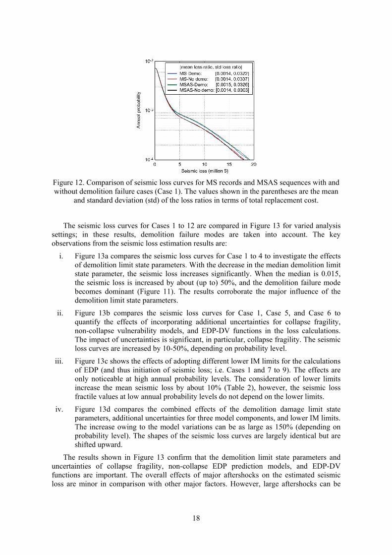
18

Figure 12. Comparison of seismic loss curves for MS records and MSAS sequences with and without demolition failure cases (Case 1). The values shown in the parentheses are the mean

and standard deviation (std) of the loss ratios in terms of total replacement cost.

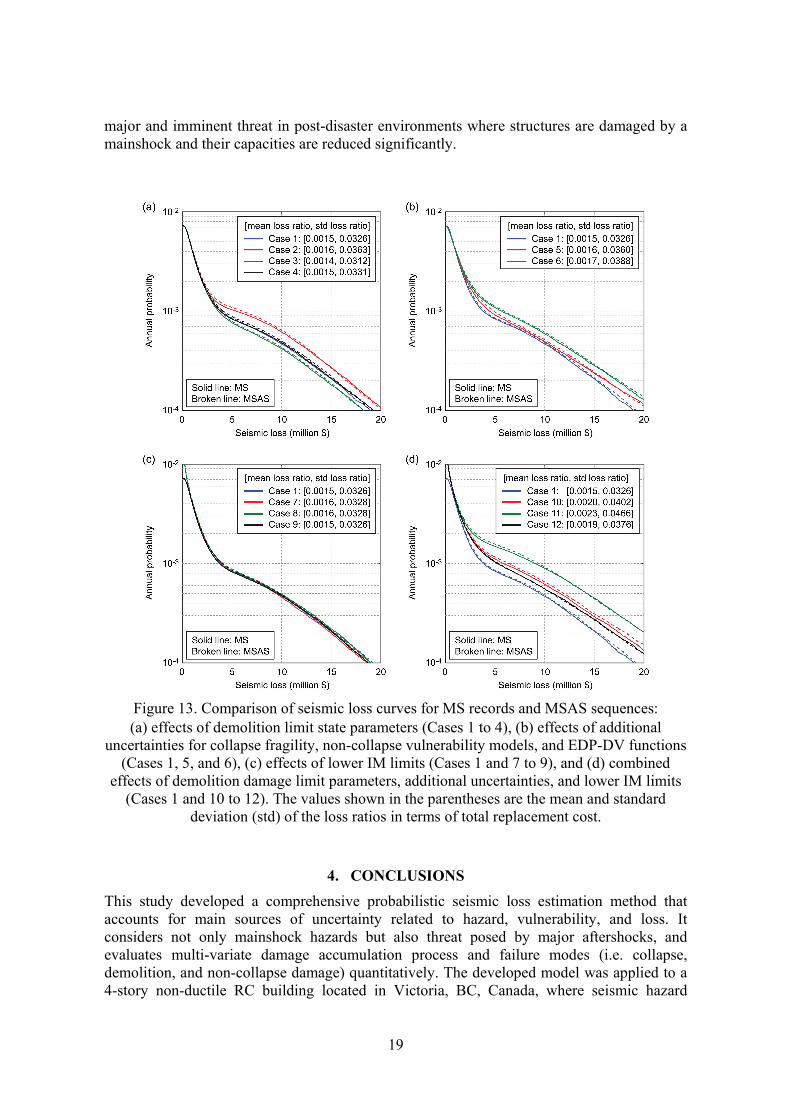
The seismic loss curves for Cases 1 to 12 are compared in Figure 13 for varied analysis settings; in these results, demolition failure modes are taken into account. The key observations from the seismic loss estimation results are:

i. Figure 13a compares the seismic loss curves for Case 1 to 4 to investigate the effects of demolition limit state parameters. With the decrease in the median demolition limit state parameter, the seismic loss increases significantly. When the median is 0.015, the seismic loss is increased by about (up to) 50%, and the demolition failure mode becomes dominant (Figure 11). The results corroborate the major influence of the demolition limit state parameters.

ii. Figure 13b compares the seismic loss curves for Case 1, Case 5, and Case 6 to quantify the effects of incorporating additional uncertainties for collapse fragility, non-collapse vulnerability models, and EDP-DV functions in the loss calculations. The impact of uncertainties is significant, in particular, collapse fragility. The seismic loss curves are increased by 10-50%, depending on probability level.

iii. Figure 13c shows the effects of adopting different lower IM limits for the calculations of EDP (and thus initiation of seismic loss; i.e. Cases 1 and 7 to 9). The effects are only noticeable at high annual probability levels. The consideration of lower limits increase the mean seismic loss by about 10% (Table 2), however, the seismic loss fractile values at low annual probability levels do not depend on the lower limits.

iv. Figure 13d compares the combined effects of the demolition damage limit state parameters, additional uncertainties for three model components, and lower IM limits. The increase owing to the model variations can be as large as 150% (depending on probability level). The shapes of the seismic loss curves are largely identical but are shifted upward.

The results shown in Figure 13 confirm that the demolition limit state parameters and uncertainties of collapse fragility, non-collapse EDP prediction models, and EDP-DV functions are important. The overall effects of major aftershocks on the estimated seismic loss are minor in comparison with other major factors. However, large aftershocks can be

19

major and imminent threat in post-disaster environments where structures are damaged by a mainshock and their capacities are reduced significantly.

Figure 13. Comparison of seismic loss curves for MS records and MSAS sequences: (a)effects of demolition limit state parameters (Cases 1 to 4), (b) effects of additional

uncertainties for collapse fragility, non-collapse vulnerability models, and EDP-DV functions (Cases 1, 5, and 6), (c) effects of lower IM limits (Cases 1 and 7 to 9), and (d) combined

effects of demolition damage limit parameters, additional uncertainties, and lower IM limits (Cases 1 and 10 to 12). The values shown in the parentheses are the mean and standard

deviation (std) of the loss ratios in terms of total replacement cost.

4. CONCLUSIONS

This study developed a comprehensive probabilistic seismic loss estimation method that accounts for main sources of uncertainty related to hazard, vulnerability, and loss. It considers not only mainshock hazards but also threat posed by major aftershocks, and evaluates multi-variate damage accumulation process and failure modes (i.e. collapse, demolition, and non-collapse damage) quantitatively. The developed model was applied to a 4-story non-ductile RC building located in Victoria, BC, Canada, where seismic hazard

20

characteristics are contributed by shallow crustal earthquakes, deep inslab earthquakes, and mega-thrust Cascadia subduction earthquakes. To reflect realistic and relevant ground motion information for Victoria, a new strong motion database from Japanese earthquakes was compiled and integrated into the existing database for MSAS sequences. The database includes records from the 2011 Tohoku earthquake, which may be regarded as the closest surrogate to the possible Mw9 Cascadia subduction earthquake. A suitable set of input ground motion records was selected using the multiple CMS method based on detailed PSHA results. A finite-element model that takes into account key hysteretic characteristics of non-ductile RC frames was adopted.

Seismic vulnerability of the RC frame was characterized through rigorous IDA and joint probabilistic modeling of multiple EDP variables (Goda and Tesfamariam [30]). The seismic loss estimation adopts a story-based damage-loss methodology. One of the major objectives in developing rigorous quantitative seismic loss estimation tools is to promote a risk-based seismic assessment approach for prioritization of seismic retrofitting.

The key findings and results from this study are:

i. In inelastic seismic demand modeling, aftershock effects are more noticeable for ResISDR than MaxISDR/PFA. This leads to moderate influence of major aftershocks on seismic loss caused by demolition (IM-DV functions). Moreover, the aftershocks effects are sensitive to the demolition damage state limits. However, when the seismic vulnerability models are integrated with seismic hazard, the aftershock effects are relatively minor in terms of overall seismic loss (1-4% increase).

ii. The most significant contributors in terms of annual seismic loss curve are the demolition limit state parameters and uncertainties of collapse fragility, non-collapse EDP prediction models, and EDP-DV functions. The increase due to the combined effects of varied model components can be as large as about 150%, depending on probability level.

The collapse in the analysis is associated with flexure or flexure-shear deterioration, and does not consider gravity load collapse due to limitations in currently available simulation models [23]. In [23], the limitation was dealt with by post-processing the drift values. Indeed, less pronounced effects of the MaxISDR/PFA demands on the aftershock risks may be partly attributed to this.

ACKNOWLEDGEMENTS

The authors acknowledge Abbie Liel for generously sharing her OpenSees model for the non-code conforming RC building. Matiyas Bezabeh’s assistance in the simulation is acknowledged. Ground motion data for Japanese earthquakes and worldwide crustal earthquakes were obtained from the K-NET/KiK-net/SK-net databases at http://www.kyoshin.bosai.go.jp/ and http://www.sknet.eri.u-tokyo.ac.jp/, and the PEER-NGA database at http://peer.berkeley.edu/nga/index.html, respectively. This work was supported by the Engineering and Physical Sciences Research Council (EP/M001067/1).

21

REFERENCES

1. Hyndman, R.D., and Rogers, G.C. (2010). Great earthquakes on Canada’s west coast: a review. Canadian Journal of Earth Sciences 47: 801–820.

2. Atkinson, G. M., and Goda, K. (2011). Effects of seismicity models and new ground-motion prediction equations on seismic hazard assessment for four Canadian cities. Bulletin of the Seismological Society of America, 101: 176–189.

3. Goldfinger, C., Nelson, C.H., Morey, A.E., Johnson, J.E., Patton, J., Karabanov, E., Gutierrez-Pastor, J., Eriksson, A.T., Gracia, E., Dunhill, G., Enkin, R.J., Dallimore, A., and Vallier, T. (2012). Turbidite event history - methods and implications for Holocene paleoseismicity of the Cascadia subduction zone. U.S. Geological Survey Professional Paper 1661–F, 170 p.

4. Onur, T., Ventura, C.E., and Finn, W.D.L. (2005). Regional seismic risk in British Columbia - damage and loss distribution in Victoria and Vancouver. Canadian Journal of Civil Engineering 32, 361–371.

5. AIR Worldwide (2013). Study of impact and the insurance and economic cost of a major earthquake in British Columbia and Ontario/Québec. Insurance Bureau of Canada, Toronto, Canada, 345 p.

6. Cornell, C.A., Jalayer, F., Hamburger, R.O., and Foutch, D.A. (2002). Probabilistic basis for 2000 SAC Federal Emergency Management Agency steel moment frame guidelines. Journal of Structural Engineering 128: 526–533.

7. Goulet, C.A., Haselton, C.B., Mitrani-Reiser, J., Beck, J.L., Deierlein, G.G., Porter, K.A., and Stewart, J.P. (2007). Evaluation of the seismic performance of a code-conforming reinforced-concrete frame building - from seismic hazard to collapse safety and economic losses. Earthquake Engineering and Structural Dynamics 36: 1973–1997.

8. Jayaram, N., Shome, N., and Rahnama, M. (2012). Development of earthquake vulnerability functions for tall buildings. Earthquake Engineering and Structural Dynamics 41, 1495–1514.

9. Vamvatsikos, D., and Cornell, C.A. (2002). Incremental dynamic analysis. Earthquake Engineering and Structural Dynamics 31: 491–514.

10. Luco, N., and Bazzurro, P. (2007). Does amplitude scaling of ground motion records result in biased nonlinear structural drift responses? Earthquake Engineering and Structural Dynamics 36: 1813–1835.

11. Baker, J.W. (2011). The conditional mean spectrum: a tool for ground motion selection. Journal of Structural Engineering 137: 322–331.

12. Goda, K., and Atkinson, G.M. (2011). Seismic performance of wood-frame houses in south-western British Columbia. Earthquake Engineering and Structural Dynamics 40: 903–924.

13. Ruiz-García, J., and Miranda, E. (2006). Evaluation of residual drift demands in regular multi-storey frames for performance-based seismic assessment. Earthquake Engineering and Structural Dynamics 35: 1609–1629.

14. Ramirez, C.M., and Miranda, E. (2012). Significance of residual drifts in building earthquake loss estimation. Earthquake Engineering and Structural Dynamics 41: 1477–1493.

15. Uma, S.R., Pampanin, S., and Christopoulos, C. (2010). Development of probabilistic framework for performance-based seismic assessment of structures considering residual deformations. Journal of Earthquake Engineering 14: 1092–1111.

16. Christopoulos, C., Pampanin, S., and Priestley, M.J.N. (2003). Performance-based seismic response of frame structures including residual deformations - part I: single-degree-of-freedom system. Journal of Earthquake Engineering 7: 97–118.

17. Li, Q., and Ellingwood, B.R. (2007). Performance evaluation and damage assessment of steel frame buildings under main shock-aftershock earthquake sequences. Earthquake Engineering and Structural Dynamics 36: 405–427.

18. Ruiz-García, J. (2012). Mainshock-aftershock ground motion features and their influence in building’s seismic response. Journal of Earthquake Engineering 16: 719–737.

19. Goda, K. and Salami, M.R. (2014). Inelastic seismic demand estimation of wood-frame houses subjected to mainshock-aftershock sequences. Bulletin of Earthquake Engineering 12: 855–874.

20. Tesfamariam, S., Goda, K., and Mondal, G. (2014). Seismic vulnerability of RC frame with unreinforced masonry infill due to mainshock-aftershock earthquake sequences. Earthquake Spectra, doi: 10.1193/042313EQS111M.

21. Haselton, C.B., Liel, A.B., Deierlein, G.G., Dean, B., and Chou, J. (2011). Seismic collapse safety of reinforced concrete buildings. I: assessment of ductile moment frames. Journal of Structural Engineering 137: 481–491.

22

22. ICBO (1967). Uniform building code. International Conference of Building Officials, Pasadena, CA.

23. Liel, A.B., and Deierlein, G.G. (2008). Assessing the collapse risk of California’s existing reinforced concrete frame structures: metrics for seismic safety decisions. Technical Report No. 166, John A. Blume Center Earthquake Engineering Center, Stanford, CA.

24. Liel, A.B., Haselton, C.B., and Deierlein, G.G. (2011). Seismic collapse safety of reinforced concrete buildings. II: comparative assessment of non-ductile and ductile moment frames. Journal of Structural Engineering 137: 492–502.

25. Uzumeri, S.M. Otani, S., and Collins, M.P. (1978). An overview of Canadian code requirements for earthquake resistant concrete buildings. Canadian Journal of Civil Engineering 5: 427–441.

26. Ibarra, L.F., Medina, R.A., and Krawinkler, H. (2005). Hysteretic models that incorporate strength and stiffness deterioration. Earthquake Engineering and Structural Dynamics 34: 1489–1511.

27. Goda, K., and Taylor, C.A. (2012). Effects of aftershocks on peak ductility demand due to strong ground motion records from shallow crustal earthquakes. Earthquake Engineering and Structural Dynamics 41: 2311–2330.

28. Goda, K. (2014). Record selection for aftershock incremental dynamic analysis. Earthquake Engineering and Structural Dynamics, doi: 10.1002/eqe.2513.

29. Porter, K.A., Kiremidjian, A.S., and LeGrue, J.S. (2001). Assembly-based vulnerability of buildings and its use in performance evaluation. Earthquake Spectra 17: 291–321.

30. Goda, K., and Tesfamariam, S. (2014). Multi-variate seismic demand modelling using copulas: application to non-ductile reinforced concrete frame in Victoria, Canada. Structural Safety (In review).

31. Jalayer, F., Asprone, D., Prota, A., and Manfredi, G. (2011). A decision support system for post-earthquake reliability assessment of structures subjected to aftershocks: an application to L’Aquila earthquake, 2009. Bulletin of Earthquake Engineering 9: 997–1014.

32. Ramirez, C.M., and Miranda, E. (2009). Building-specific loss estimation methods & tools for simplified performance-based earthquake engineering. Technical Report No. 171, John A. Blume Center Earthquake Engineering Center, Stanford, CA.