Embed Size (px)
Citation preview
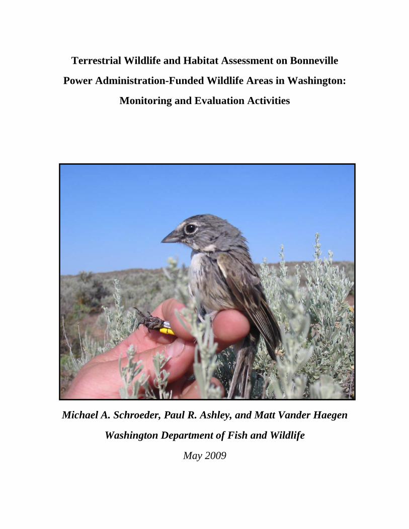
Terrestrial Wildlife and Habitat Assessment on Bonneville
Power Administration-Funded Wildlife Areas in Washington:
Monitoring and Evaluation Activities
Michael A. Schroeder, Paul R. Ashley, and Matt Vander Haegen
Washington Department of Fish and Wildlife
May 2009

2
TABLE OF CONTENTS TABLE OF CONTENTS.......................................................................................................2 EXECUTIVE SUMMARY ...................................................................................................5 INTRODUCTION .................................................................................................................8
VISION............................................................................................................................8 WASHINGTON DEPARTMENT OF FISH AND WILDLIFE .....................................8 NORTHWEST POWER PLANNING COUNCIL........................................................11
Purpose.....................................................................................................................11 The Importance of Monitoring and Evaluation .......................................................15 Adaptive Management .............................................................................................17
MONITORING AND EVALUATION ...............................................................................18 FOCAL SPECIES AND HABITATS ...........................................................................18
Justification..............................................................................................................18 Description of Focal Habitats ..................................................................................19 Description of Focal Species ...................................................................................20
HABITAT EVALUATION PROCEDURES................................................................34 General Description .................................................................................................34 Methods for Open Habitats......................................................................................37 Methods for Forest and Riparian Habitats ...............................................................44 Application of HEP Data to Wildlife.......................................................................46
MODIFIED HABITAT ASSESSMENT PROCEDURES............................................49 Justification for Modification ..................................................................................49 Habitat Methods.......................................................................................................51
WILDLIFE MONITORING AND EVALUATION .....................................................53 Pygmy Rabbit...........................................................................................................54 Beaver ......................................................................................................................54 Western Gray Squirrel .............................................................................................55 Big Game .................................................................................................................55 Prairie Grouse ..........................................................................................................56 Great Blue Heron .....................................................................................................56 Mallard.....................................................................................................................56 Owls and Woodpeckers ...........................................................................................57 Songbirds .................................................................................................................57 Miscellaneous Surveys.............................................................................................60
SAGEBRUSH FLAT WILDLIFE AREA...........................................................................62 DESCRIPTION..............................................................................................................62 UPPER MIDDLE MAINSTEM SUBBASIN ...............................................................65 MONITORING AND EVALUATION .........................................................................66
Habitat......................................................................................................................66 Mule Deer ................................................................................................................68 Prairie Grouse ..........................................................................................................69 General Bird Surveys...............................................................................................70 Miscellaneous Surveys.............................................................................................75
SCOTCH CREEK WILDLIFE AREA................................................................................77 DESCRIPTION..............................................................................................................77

3
UPPER MIDDLE MAINSTEM AND UPPER COLUMBIA SUBBASINS................80 MONITORING AND EVALUATION .........................................................................82
Habitat......................................................................................................................82 Mule Deer and White-tailed Deer............................................................................84 Prairie Grouse ..........................................................................................................84 General Bird Surveys...............................................................................................86
BIRD SPECIES .............................................................................................................88 SWANSON LAKES WILDLIFE AREA ............................................................................93
DESCRIPTION..............................................................................................................93 CRAB CREEK SUBBASIN..........................................................................................97 MONITORING AND EVALUATION .........................................................................97
Habitat......................................................................................................................97 Mule Deer ................................................................................................................98 Prairie Grouse ..........................................................................................................98 General Bird Surveys.............................................................................................100 Miscellaneous Surveys...........................................................................................104
SUNNYSIDE WILDLIFE AREA .....................................................................................105 DESCRIPTION............................................................................................................105 YAKIMA SUBBASIN ................................................................................................106 MONITORING AND EVALUATION .......................................................................107
Elk ..........................................................................................................................107 Mule Deer ..............................................................................................................108 Miscellaneous Surveys...........................................................................................108
WENAS WILDLIFE AREA..............................................................................................109 DESCRIPTION............................................................................................................109 YAKIMA SUBBASIN ................................................................................................111 FOCAL ........................................................................................................................111 MONITORING AND EVALUATION .......................................................................112
Habitat....................................................................................................................112 Elk ..........................................................................................................................113 Mule Deer ..............................................................................................................114 Bighorn Sheep........................................................................................................115 Prairie Grouse ........................................................................................................115 General Bird Surveys.............................................................................................116
ASOTIN CREEK WILDLIFE AREA...............................................................................119 DESCRIPTION............................................................................................................119 ASOTIN SUBBASIN ..................................................................................................121 MONITORING AND EVALUATION .......................................................................121
Habitat....................................................................................................................121 Elk ..........................................................................................................................124 Mule Deer ..............................................................................................................125 Bighorn Sheep........................................................................................................125 Great Blue Heron ...................................................................................................125 Prairie Grouse ........................................................................................................125 General Bird Surveys.............................................................................................125
BIRDS/POINT.............................................................................................................126

4
SHILLAPOO WILDLIFE AREA......................................................................................127 DESCRIPTION............................................................................................................127 LOWER COLUMBIA TRIBUTARIES SUBBASIN (LCTS)....................................129 MONITORING AND EVALUATION .......................................................................129
Deer........................................................................................................................129 Great Blue Heron ...................................................................................................129 Miscellaneous Surveys...........................................................................................129
DESERT WILDLIFE AREA.............................................................................................130 DESCRIPTION............................................................................................................130 CRAB CREEK SUBBASIN........................................................................................131 MONITORING AND EVALUATION .......................................................................131
Habitat....................................................................................................................131 Deer........................................................................................................................131 Great Blue Heron ...................................................................................................131 Miscellaneous Surveys...........................................................................................132
DISCUSSION AND RECOMENDATIONS ....................................................................133 LITERATURE CITED ......................................................................................................140 APPENDIX A: ACRONYMS AND ABBREVIATIONS ...............................................149 APPENDIX B: SCIENTIFIC NAMES ............................................................................151
PLANTS ......................................................................................................................151 MAMMALS ................................................................................................................153 BIRDS..........................................................................................................................154 REPTILES AND AMPBIBIANS................................................................................160
APPENDIX C: SAMPLE DATA FORMS ......................................................................161
5
EXECUTIVE SUMMARY
The Washington Department of Fish and Wildlife strives to manage its wildlife areas to protect and provide the habitat necessary to support healthy and diverse fish and wildlife populations, and provide compatible recreational opportunities. Effective management of fish and wildlife, and habitats upon which they depend, requires an adaptive approach. The Northwest Power Planning Council stated “management actions must be taken in an adaptive, experimental manner because ecosystems are inherently variable and highly complex. These include using experimental designs and techniques as part of management actions, and integrating monitoring and research with management actions to evaluate effects on the ecosystem.” Monitoring and evaluation are critical in this process because they provide the information necessary to evaluate management activities in the past and to improve management activities in the future.
Habitat protection and enhancement is the fundamental strategy used by the Bonneville Power Administration to compensate for habitat lost during the construction and operation of hydroelectric projects in the Columbia Basin. Habitat monitoring and evaluation procedures are used to make these determinations based on documented relationships between focal habitats and species. Focal habitats used for this habitat evaluation methodology include shrubsteppe (grassland ecosystem in which shrubs usually contribute to the overstory), interior riparian wetlands (diverse mixture of herbaceous vegetation, shrubs, and trees in close proximity to water), and Ponderosa pine (relatively open and dry forest type with a variable density of Ponderosa pine, but usually characterized by an understory of bunchgrasses, forbs, and shrubs). The rationale for concentrating on focal habitats is to draw attention to ecosystems most in need of conservation.
Focal species were selected with a rational similar to that used for focal habitats. Focal species reflect the features and conditions necessary in a functioning ecosystem. In some instances, extirpated or nearly extirpated species (e.g., pygmy rabbit, sharp-tailed grouse, greater sage-grouse) can be included as focal species, because their populations can potentially be re-established and/or enhanced they are indicative of desirable habitat conditions. In other instances, focal species can be selected, based on localized management priorities, or based on the assumption that they provide insights into the integrity of the larger ecological system to which they belong, hence serving as ‘umbrella’ or ‘indicator’ species. The distribution and abundance of these focal species must be regularly monitored and the data used in evaluations of: 1) the presumed relationship between the focal species and its primary habitat; 2) the usefulness of the species in reflecting the ‘health’ of the larger ecosystem; and 3) adaptive management strategies.
Focal mammal species considered in this report include elk, mule deer, bighorn sheep, pygmy rabbit, beaver, and western gray squirrel. Monitoring of elk, mule deer, and bighorn sheep has followed WDFW regional big game survey protocols. These include annual population estimates, classification by sex and age composition, survival rates, and trend analyses. Aerial surveys and harvest data provide most of this information, but local pellet count transects have also been employed. Pygmy rabbit
6
surveys adhere to protocols developed in conjunction with WDFW and the Pygmy Rabbit Recovery Team and include population estimates, identification of distribution, trend analyses, and habitat condition assessments. Beaver surveys have been coordinated with other WDFW regional aerial surveys to include population estimates, documentation of lodges, population distribution, and trend analyses. Western gray squirrel surveys follow standard procedures identified by the WDFW for specific wildlife areas where squirrel distribution is possible. Once squirrel presence is identified, nest tree surveys for western gray squirrels are conducted.
Focal bird species include great blue heron, mallard, sharp-tailed grouse, greater sage-grouse, flammulated owl, Lewis’ woodpecker, white-headed woodpecker, gray flycatcher, willow flycatcher, red-eyed vireo, pygmy nuthatch, sage thrasher, yellow warbler, yellow-breasted chat, grasshopper sparrow, Brewer’s sparrow, sage sparrow, and red-winged blackbird. Specific sampling techniques include annual nest colony surveys for herons, mid-winter and summer aerial surveys for mallards (and other migratory waterfowl), lek searches and pellet counts for sharp-tailed grouse and greater sage-grouse, call surveys for owls and woodpeckers, and breeding bird surveys, nest searches, and winter surveys for songbirds. Standard protocols are available for most species.
Monitoring and evaluation of wildlife areas occurs at different levels of intensity. At the simplest level, there are assessments of progress of individual operations and maintenance projects. Mitigation and enhancement projects are also being monitored with designated sampling procedures developed and approved by WDFW. Focal wildlife species and habitats are being monitored using sampling procedures from national, subbasin, and WDFW regional level surveys, with application to each wildlife area. Monitoring and evaluation are being conducted to assure that mitigation and enhancement activities and overall management of BPA-funded wildlife areas is contributing to the continued health of the local ecosystem and its associated wildlife and habitats.
The monitoring and evaluation strategy will be enhanced and expanded on the wildlife areas. The purpose of this strategy will be to collect data on habitats and species that permits: 1) temporal evaluations of habitat suitability and species abundance; 2) tests of assumptions of the umbrella species concept; 3) examination of specific relationships between focal species and habitats; 4) determination of the habitat enhancement credits due to the Bonneville Power Administration; 5) consideration of alternate methods for monitoring both habitat and wildlife; and 6) integration of monitoring and evaluation efforts across all BPA-funded wildlife areas.
This report outlines the background of major BPA-funded wildlife areas in Washington. These Wildlife Areas, and their associated units, include Asotin Creek, Desert, Sagebrush Flat, Scotch Creek, Shillapoo, Sunnyside, Swanson Lakes, and Wenas. The management of these wildlife areas is integrated with, and supported by, numerous subbasin plans, within the Columbia River Basin watershed. These subbasin plans, produced by the Northwestern Power Planning Council, include the Asotin, Crab Creek, Lower Columbia Tributaries, Okanogan, Upper Columbia, Upper Middle Mainstem, and Yakima. This final report outlines some of the information available on focal species and

7
habitats, as well as some of the assumptions made concerning their usefulness in the overall monitoring and evaluation strategy. This report also describes some of the available results from past monitoring activities, as well as insights into a monitoring and evaluation strategy for the future.
Recommended citation:
Schroeder, M. A., P. R. Ashley, and M. Vander Haegen. 2009. Terrestrial wildlife and habitat assessment on Bonneville Power Administration-funded Wildlife Areas in the State of Washington: Monitoring and evaluation activities of the past and recommendations for the future. Washington Department of Fish and Wildlife, Olympia, Washington.
8
INTRODUCTION
VISION
This report has been designed to examine the history of terrestrial wildlife and habitat monitoring efforts on Wildlife Areas managed by the Washington Department of Fish and Wildlife (WDFW), particularly those funded by the Bonneville Power Administration (BPA). Our intention was to evaluate data already collected on the Wildlife Areas and design and implement a consistent monitoring and evaluation procedure for the future. With that in mind, this report first examines the mandates of the principal agencies involved in management of these Wildlife Areas. We focus primarily on goals, objectives, and strategies that pertain to the monitoring and evaluation of fish and wildlife resources, and the habitats upon which they depend. We then examine the specific Wildlife Areas that receive funding from the Bonneville Power Administration. This examination includes basic information on Wildlife Area configuration and history, but most importantly on the management goals, objectives, and strategies for their wildlife and habitats. These objectives not only include those stated in the management plans for the specific Wildlife Areas, but also those stated in the relevant Columbia River Basin subbasin plans that were published by the Northwest Power Planning Council. We then examine available data for each Wildlife Area, providing analysis when appropriate. Finally, we provide details for a continuing monitoring and evaluation strategy for the BPA-funded Wildlife Areas.
A great deal of thought and effort has been expended by countless individuals on the subjects of management, mitigation, monitoring, and evaluation of Columbia Basin ecosystems. By necessity, we borrowed heavily from their voluminous reports and publications, as illustrated by the frequent quotations and references. Any failure on our part to adequately reference the appropriate and/or original sources for the information was accidental. To shorten the length of the report, we regularly used acronyms and abbreviations (see Appendix A for list). Scientific names for plants and animals are in Appendix B.
WASHINGTON DEPARTMENT OF FISH AND WILDLIFE
The Washington Department of Fish and Wildlife serves Washington’s citizens by protecting, restoring and enhancing fish and wildlife and their habitats, while providing sustainable and wildlife-related recreational and commercial opportunities (WDFW 2004b).
The first goal listed in the WDFW strategic plan is to ensure healthy and diverse fish and wildlife populations and habitats within the state of Washington (WDFW 2004b). There are several objectives listed in association with this goal including:
1. Develop, integrate and disseminate sound fish, wildlife and habitat science.
9
2. Protect, restore and enhance fish and wildlife populations and their habitats.
3. Ensure WDFW activities, programs, facilities and lands are consistent with local, state and federal regulations that protect and recover fish, wildlife and their habitats.
4. Influence the decisions of others that affect fish, wildlife and their habitats.
5. Minimize adverse interactions between humans and wildlife.
The second goal listed in the WDFW strategic plan is to support sustainable fish and wildlife-related opportunities (WDFW 2004b). There are three objectives listed in association with this goal including:
1. Provide sustainable fish and wildlife-related recreational and commercial opportunities compatible with maintaining healthy fish and wildlife populations and habitats.
2. Work with Tribal governments to ensure fish and wildlife management objectives are achieved.
3. Improve the economic well-being of Washington by providing diverse, high quality recreational and commercial opportunities.
The third goal listed in the WDFW strategic plan is to insure operational excellence and professional service (WDFW 2004b). There are four objectives listed in association with this goal including:
1. Provide excellent professional service.
2. Improve the effectiveness and efficiency of WDFW's operational and support activities.
3. Provide sound operational management of WDFW lands, facilities and access sites.
4. Develop Information Systems infrastructure and coordinate data systems to provide access to services and information.
5. Recruit, develop and retain a diverse workforce with high professional standards.
6. Maintain a safe work environment.
7. Reconnect with those interested in Washington's fish and wildlife.
10
In association with these stated goals, there are many strategies that are relevant to the management of fish and wildlife resources, and the habitats supporting them, on state-managed Wildlife Areas (WDFW 2004b). Some of these are listed below:
“WDFW will provide leadership in developing, integrating and disseminating the best applied science for use in policy and management decisions affecting fish and wildlife and their habitats” (WDFW 2004b:22).
“WDFW will continue to improve access to priority scientific data and information for key partners and the public” (WDFW 2004b:22).
“WDFW will utilize multi-species, habitat-based approaches to resource management and conservation to improve the effectiveness in maintaining healthy populations and recovering those that are not” (WDFW 2004b:22).
“WDFW will manage its wildlife areas to protect and provide habitat to achieve healthy and diverse fish and wildlife populations, and provide for compatible fish and wildlife recreational opportunities” (WDFW 2004b:22).
“WDFW will ensure that Department actions, lands and facilities meet local, state and federal regulations that protect and recover fish, wildlife and their habitats. Impairments to fish and wildlife recovery on WDFW lands and facilities will be identified and addressed” (WDFW 2004b:24).
“WDFW will collaborate with landowners, local governments, land management agencies and tribal, state and federal governments that influence decisions important to fish, wildlife and habitat” (WDFW 2004b:24).
“WDFW will work with other land management entities to identify where habitat protection can occur most effectively and efficiently. WDFW will work with these entities to protect priority habitats through numerous strategies including incentives, easements, agreements, and acquisitions” (WDFW 2004b:24).
“WDFW will provide technical review and technical assistance as well as provide access to information and management recommendations to assist others in protecting and restoring fish, wildlife and their habitats. WDFW will actively seek feedback on the value of the information and technical assistance it provides in order to improve service” (WDFW 2004b:24).
11
“WDFW will provide sustainable fish and wildlife opportunities through effective management decisions while improving the economic well-being of the state” (WDFW 2004b:25).
“WDFW will learn more about what fish and wildlife opportunities the public is interested in to develop ways to meet this interest while maintaining healthy fish and wildlife populations” (WDFW 2004b:25).
“WDFW will increase the watchable fish and wildlife opportunities and information it provides to the public” (WDFW 2004b:25).
“WDFW will continue to foster and improve volunteer activities and partnerships that assist in achieving mutual goals of protecting and enhancing fish and wildlife and their habitats” (WDFW 2004b:30).
“Strategies will be developed to ensure sound sustainable operational management is based on solid, reliable, easily accessible information and scientific data” (WDFW 2004b:30).
NORTHWEST POWER PLANNING COUNCIL
Purpose
The Northwest Power Planning Council was authorized in 1980 by the United States Congress “to prepare a program to protect, mitigate and enhance fish and wildlife of the Columbia River Basin that have been affected by the construction and operation of hydroelectric dams while also assuring the Pacific Northwest an adequate, efficient, economical and reliable power supply” (NPPC 2000:7). The NPPC provides guidance and recommendations to the Bonneville Power Administration (BPA) for expenditures to mitigate the impact of 29 hydroelectric dams and one non-federal nuclear power plant on fish and wildlife in the Columbia River Basin. The funding is provided by BPA from the sale of electricity and is targeted toward the protection, mitigation, and enhancement of fish and wildlife. The program also “includes procedures for monitoring and evaluating biological benefits gained by actions taken under the program. The evaluation process feeds information back into the program planning and project review process, with adaptive management mechanisms for revising program objectives or actions if what has been adopted proves unsuccessful” (NPPC 2000:7).
The NPPC has an established program for fish and wildlife in the Columbia River Basin (NPPC 2000). This program includes provisions for the overall Columbia River Basin, such as a ‘vision’ (NPCC 2000:13).
“The vision for this program is a Columbia River ecosystem that sustains an abundant, productive, and diverse community of fish and wildlife, mitigating across the basin for the adverse effects to fish and wildlife caused by the development and operation of the hydrosystem and providing the benefits from fish and wildlife valued by the people of the
12
region. This ecosystem provides abundant opportunities for tribal trust and treaty right harvest and for non-tribal harvest and the conditions that allow for the recovery of the fish and wildlife affected by the operation of the hydrosystem and listed under the Endangered Species Act.
Whenever feasible, this program will be accomplished by protecting and restoring the natural ecological functions, habitats, and biological diversity of the Columbia River Basin. In those places where this is not feasible, other methods that are compatible with naturally reproducing fish and wildlife populations will be used. Where impacts have irrevocably changed the ecosystem, the program will protect and enhance the habitat and species assemblages compatible with the altered ecosystem. Actions taken under this program must be cost-effective and consistent with an adequate, efficient, economical and reliable electrical power supply.”
Several assumptions also underlie the NPPC (2000:13) vision including:
“No single activity is sufficient to recover and rebuild fish and wildlife species in the Columbia River Basin. Successful protection, mitigation, and recovery efforts must involve a broad range of strategies for habitat protection and improvement, hydrosystem reform, artificial production, and harvest management.
This is a habitat-based program, rebuilding healthy, naturally producing fish and wildlife populations by protecting, mitigating, and restoring habitats and the biological systems within them, including anadromous fish corridors. Artificial production and other non-natural interventions should be consistent with the central effort to protect and restore habitat and avoid adverse impacts to native fish and wildlife species.
Management actions must be taken in an adaptive, experimental manner because ecosystems are inherently variable and highly complex. This includes using experimental designs and techniques as part of management actions, and integrating monitoring and research with those management actions to evaluate their effects on the ecosystem.
There is an obligation to provide fish and wildlife mitigation where habitat has been permanently lost due to hydroelectric development.”
The NPPC has an established scientific foundation for their fish and wildlife program in the Columbia River Basin (NPPC 2000). This includes the foundational principle of relying on the best available science, as well as the following specific principles (NPPC 2000:15):
“The abundance, productivity and diversity of organisms are integrally linked to the characteristics of their ecosystems.
13
Ecosystems are dynamic, resilient and develop over time.
Biological systems operate on various spatial and time scales that can be organized hierarchically.
Habitats develop, and are maintained, by physical and biological processes.
Species play key roles in developing and maintaining ecological conditions.
Biological diversity allows ecosystems to persist in the face of environmental variation.
Ecological management is adaptive and experimental.
Ecosystem function, habitat structure and biological performance are affected by human actions.”
The NPCC has many objectives regarding the protection, mitigation, management, and enhancement of fish and wildlife in the Columbia River Basin. These include overarching objectives for the overall Columbia River Basin, as well as many specific objectives for provinces and subbasins within the overall basin. Although these “specific objectives will be considered as guidance for subbasin planning” (http://www.nwcouncil.org/fw/subbasinplanning/), some of the more general objectives are listed below (NPCC 2000:16):
“A Columbia River ecosystem that sustains an abundant, productive, and diverse community of fish and wildlife.
Mitigation across the basin for the adverse effects to fish and wildlife caused by the development and operation of the hydrosystem.
Sufficient populations of fish and wildlife for abundant opportunities for tribal trust and treaty right harvest and for non-tribal harvest.
Recovery of the fish and wildlife affected by the development and operation of the hydrosystem that are listed under the Endangered Species Act.”
With specific reference to direct and indirect losses of wildlife through the construction and operation of hydrosystems, the NPPC (2000:17) includes “implementation projects to obtain and protect habitat units in mitigation for these calculated construction/inundation losses. Operational and secondary losses have not been estimated or addressed. The program includes a commitment to mitigate for these losses. More specific wildlife objectives are:”

14
“Quantify wildlife losses caused by the construction, inundation, and operation of the hydropower projects.
Develop and implement habitat acquisition and enhancement projects to fully mitigate for identified losses.
Coordinate mitigation activities throughout the basin and with fish mitigation and restoration efforts, specifically by coordinating habitat restoration and acquisition with aquatic habitats to promote connectivity of terrestrial and aquatic areas.
Maintain existing and created habitat values.
Monitor and evaluate habitat and species responses to mitigation actions.”
“Strategies are plans of action to accomplish the biological objectives” (NPPC 2000:19). Some of the basic recommended strategies include:
“Where the habitat for a target population is largely intact, then the biological objectives for that habitat will be to preserve the habitat and restore the population of the target species up to the sustainable capacity of the habitat.
Where the habitat for a target population is absent or severely diminished, but can be restored through conventional techniques and approaches, then the biological objective for that habitat will be to restore the habitat with the degree of restoration depending on the biological potential of the target population.
Where the habitat for a target population is absent or substantially diminished and cannot reasonably be fully restored, then the biological objective for that habitat will depend on the biological potential of the target species.
Where habitat for a target population is irreversibly altered or blocked, and therefore there are no opportunities to rebuild the target population by improving its opportunities for growth and survival in other parts of its life history, then the biological objective will be to provide a substitute. In the case of wildlife, where the habitat is inundated, substitute habitat would include setting aside and protecting land elsewhere that is home to a similar ecological community.
Identify the current condition and biological potential of the habitat, and then protect or restore it to the extent described in the biological objectives.
15
Complete the current mitigation program for construction and inundation losses and include wildlife mitigation for all operational losses as an integrated part of habitat protection and restoration.”
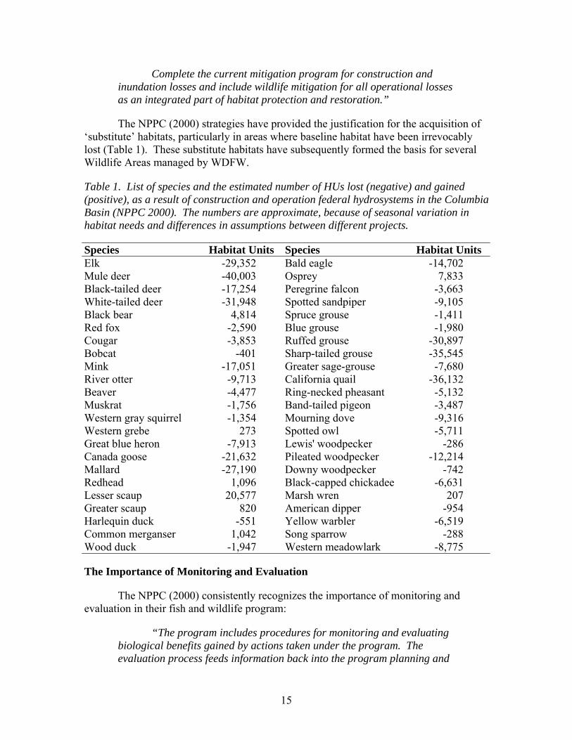
The NPPC (2000) strategies have provided the justification for the acquisition of ‘substitute’ habitats, particularly in areas where baseline habitat have been irrevocably lost (Table 1). These substitute habitats have subsequently formed the basis for several Wildlife Areas managed by WDFW.
Table 1. List of species and the estimated number of HUs lost (negative) and gained (positive), as a result of construction and operation federal hydrosystems in the Columbia Basin (NPPC 2000). The numbers are approximate, because of seasonal variation in habitat needs and differences in assumptions between different projects.
Species Habitat Units Species Habitat Units Elk -29,352 Bald eagle -14,702 Mule deer -40,003 Osprey 7,833 Black-tailed deer -17,254 Peregrine falcon -3,663 White-tailed deer -31,948 Spotted sandpiper -9,105 Black bear 4,814 Spruce grouse -1,411 Red fox -2,590 Blue grouse -1,980 Cougar -3,853 Ruffed grouse -30,897 Bobcat -401 Sharp-tailed grouse -35,545 Mink -17,051 Greater sage-grouse -7,680 River otter -9,713 California quail -36,132 Beaver -4,477 Ring-necked pheasant -5,132 Muskrat -1,756 Band-tailed pigeon -3,487 Western gray squirrel -1,354 Mourning dove -9,316 Western grebe 273 Spotted owl -5,711 Great blue heron -7,913 Lewis' woodpecker -286 Canada goose -21,632 Pileated woodpecker -12,214 Mallard -27,190 Downy woodpecker -742 Redhead 1,096 Black-capped chickadee -6,631 Lesser scaup 20,577 Marsh wren 207 Greater scaup 820 American dipper -954 Harlequin duck -551 Yellow warbler -6,519 Common merganser 1,042 Song sparrow -288 Wood duck -1,947 Western meadowlark -8,775
The Importance of Monitoring and Evaluation
The NPPC (2000) consistently recognizes the importance of monitoring and evaluation in their fish and wildlife program:
“The program includes procedures for monitoring and evaluating biological benefits gained by actions taken under the program. The evaluation process feeds information back into the program planning and
16
project review process, with adaptive management mechanisms for revising program objectives or actions if what has been adopted proves unsuccessful” (NPPC 2000:11).
“Management actions must be taken in an adaptive, experimental manner because ecosystems are inherently variable and highly complex. This includes using experimental designs and techniques as part of management actions, and integrating monitoring and research with those management actions to evaluate their effects on the ecosystem” (NPPC 2000:13).
“Biological objectives describe physical and biological changes needed to achieve the vision, based on the information we now have and thereby fulfill the vision. Biological objectives have two components: (1) biological performance, describing responses of populations to habitat conditions, described in terms of capacity, abundance, productivity and life history diversity, and (2) environmental characteristics, which describe the environmental conditions or changes sought to achieve the desired population characteristics. Where possible, biological objectives are intended to be empirically measurable and based on an explicit scientific rationale. Objectives at the basin level are more qualitative, but objectives should become increasingly quantitative and measurable at the province and subbasin levels. These basinwide objectives will help determine the amount of change needed across the basin to fulfill the vision. They will also help determine the cost effectiveness of program strategies, and provide a basis for monitoring, evaluation and accountability” (NPPC 2000:16).
Monitor and evaluate habitat and species responses to mitigation actions” (NPPC 2000:17).
“These objectives and the strategies that follow are to be used as guidance for developing province and subbasin plans, as the basis for development of more specific objectives, and as a basis for Council recommendations to the Bonneville Power Administration regarding project funding. Proposed measures will be evaluated for consistency with these objectives and strategies. A primary function of the monitoring and evaluation components of this program is to measure progress toward achieving these objectives” (NPPC 2000:18).
“Habitat enhancement credits should be provided to Bonneville when habitat management activities funded by Bonneville lead to a net increase in habitat value when compared to the level identified in the baseline habitat inventory and subsequent habitat inventories. This determination should be made through the periodic monitoring of the project site using the Habitat Evaluation Procedure (HEP) methodology.
17
Bonneville should be credited for habitat enhancement efforts at a ratio of one habitat unit credited for every habitat unit gained” (NPPC 2000:31).
“The purpose of the monitoring and evaluation strategies is to assure that the effects of actions taken under this program are measured, that these measurements are analyzed so that we have better knowledge of the effects of the action, and that this improved knowledge is used to choose future actions” (NPPC 2000:32).
Adaptive Management
The adaptive management cycle is a fundamental component of NPPC plans (NPPC 2004a-g). The basic cycle consists of four steps (Ringold et al. 1996): 1) Resource objectives are developed to describe the desired condition; 2) Management is designed to meet the resource objectives; 3) Resources are monitored to evaluate whether the management objective has been met; and 4) Management is altered if objectives have not been reached.
Monitoring methods should be driven by management objectives, used especially when there are opportunities for adaptive management. If no alternative management options are available, it may not be useful to expend resources for monitoring (this does not preclude general inventories). In such cases, most resource monitoring should be directed towards opportunities where management options are available.
18
MONITORING AND EVALUATION
A broad goal in resource management is protection of the full range of biodiversity with the aid of ‘conservation networks’ that consider habitat condition of core areas, habitat quantity, patch connectivity, and buffer zones. Although management at the ecoregional scale can consider broad goals and objectives, management at the subbasin and wildlife area scale focuses on quantity, quality, and configuration of important habitats and the individual species and the species guilds they reflect.
FOCAL SPECIES AND HABITATS
Justification
Lambeck (1997) recommends monitoring and evaluation of focal species whose life history requirements for persistence define the habitat attributes that must be present if a landscape is to meet the requirements for all species that occur there. The key characteristic of a focal species is that its status and trend provide insights into the integrity of the larger ecological system to which it belongs; in essence they should function as ‘umbrella’ species. Each subbasin plan (see NPPC 2004a-g for examples) includes a list of focal species, to be considered in monitoring and evaluation. Species listed in mitigation losses for dams are not necessarily the species selected as ‘focal’ species. Similarly, some species listed as ‘priorities’ in Wildlife Area management plans were not selected necessarily as focal species for the subbasin/s in which the Wildlife Areas were located. Likewise, focal species in one subbasin were not necessarily considered in other subbasins, even if the species were present.
The rationale for using focal species is to draw immediate attention to habitat features and conditions most in need of conservation, or most important in a functioning ecosystem (NPPC 2000). In some instances, extirpated or nearly extirpated species (e.g., pygmy rabbit, sharp-tailed grouse, greater sage-grouse) can be included as focal species, because their populations potentially can be re-established and/or enhanced and they are indicative of desirable habitat conditions. The selection of these focal species, and the focal habitats upon which they reflect and depend, has been based on a variety of sources including PIF, Washington Priority Habitats and Species, Washington GAP Analysis Project, National Wetland Inventory, Ecoregional Conservation Assessment, and IBIS (Andelman et al. 1999, Ashley and Stovall 2004a,b).
A ‘coarse filter/fine filter’ approach was used to select focal habitats (Haufler 2002). The coarse filter compares the current availability of focal species habitat against historic availability to evaluate the relative status of a given habitat and its suite of obligate species. The coarse filter habitat analysis was combined with a single species or ‘fine filter’ analysis of one or more obligate species to further ensure that species viability for the suite of species was maintained. The following key principles/assumptions were used to guide selection of focal habitats: 1) Focal habitats were identified by WDFW at the coarse filter scale where they can be used to evaluate ecosystem health and establish management priorities; and 2) Focal species/guilds were selected to represent focal

19
habitats and to infer and/or measure response to changing habitat conditions at the fine filter or subbasin scale.
Description of Focal Habitats
Although many different habitats are addressed in subbasin plans within the Columbia River Basin, only three focal habitats were selected for this effort, including Shrubsteppe, Interior Riparian Wetlands, and Ponderosa Pine Forest (NPPC 2000). Ponderosa Pine Forest can be defined as a relatively open and dry forest type with a variable density of Ponderosa pine, but usually characterized by an understory consisting of bunchgrasses, forbs, and shrubs. The overstory may include other trees, such as oak and Douglas fir. Shrubsteppe can be defined as a grassland ecosystem, in which shrubs usually contribute to the overstory. Because grassland habitats that have few, if any, shrubs also can be defined botanically as shrubsteppe, there is some ambiguity about the definition of Shrubsteppe (used here) versus grassland (used in wildlife area management by WDFW). Consequently, interior grasslands were combined with shrubsteppe habitats in this report to form a single Shrubsteppe category. In the case of the Asotin Creek Wildlife Area (ACWA), the Wildlife Area with the most extensive grasslands, the combination of grassland and shrubsteppe into a single Shrubsteppe category had little effect, because most of the same focal species were considered in each of the ‘separate’ grassland and shrubsteppe habitats. Riparian Wetland can be defined as a diverse mixture of herbs, shrubs, and trees (many obligate and facultative species) in close proximity to water. Once again, herbaceous wetlands were combined within the Interior Riparian Wetland category, because the delineation between the two habitats was ambiguous and some of the same focal species were used in both descriptions. Heavily forested and/or high elevation habitats were not addressed in this report, because the Wildlife Areas funded for BPA-mitigation were, by design, relatively low in elevation.
Monitoring of focal habitats employs a stratified random sampling design which, at a minimum, identifies plant species composition; percent canopy cover by species and by vegetation layer (ground cover, biological crust, grasses, forbs, shrubs, trees); plant species height, diameter, and density; tree diameter at breast height, and height; percent cover of rock, litter, woody material, and bare ground; and number and classification of snags. Sampling incorporates multiple methods, including a standard Habitat Evaluation Procedure (HEP), but allows the testing and application of alternate procedures designed to provide habitat information accurately and efficiently. For operation and maintenance projects, such as roadwork, culvert removal, fencing changes, construction, etc., before and after photographs serve to document the progress and completion of the project. Seasonal or annual photographs of work in progress are used to document long-term projects. Projects involving restoration activities, such as disking, seeding, planting, herbicide application, biological control, irrigation, and controlled burning require more extensive documentation of progress. Wildlife area staff periodically monitor projects associated with seasonal manipulations to change plant species composition or plant succession, by using standardized sampling procedures to identify the progress and results of manipulations.
20
Description of Focal Species
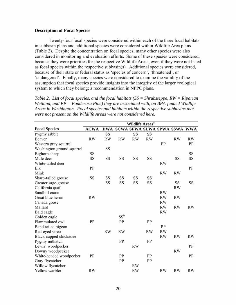
Twenty-four focal species were considered within each of the three focal habitats in subbasin plans and additional species were considered within Wildlife Area plans (Table 2). Despite the concentration on focal species, many other species were also considered in monitoring and evaluation efforts. Some of these species were considered, because they were priorities for the respective Wildlife Areas, even if they were not listed as focal species within the respective subbasin(s). Additional species were considered, because of their state or federal status as ‘species of concern’, ‘threatened’, or ‘endangered’. Finally, many species were considered to examine the validity of the assumption that focal species provide insights into the integrity of the larger ecological system to which they belong; a recommendation in NPPC plans.
Table 2. List of focal species, and the focal habitats (SS = Shrubsteppe, RW = Riparian Wetland, and PP = Ponderosa Pine) they are associated with, on BPA-funded Wildlife Areas in Washington. Focal species and habitats within the respective subbasins that were not present on the Wildlife Areas were not considered here.
Wildlife Areasa Focal Species ACWA DWA SCWA SFWA SLWA SPWA SSWA WWAPygmy rabbit SS SS SS Beaver RW RW RW RW RW RW RW Western gray squirrel PP PP Washington ground squirrel SS Bighorn sheep SS SS Mule deer SS SS SS SS SS SS SS White-tailed deer RW Elk PP PP Mink RW RW Sharp-tailed grouse SS SS SS SS SS Greater sage-grouse SS SS SS SS SS SS California quail RW Sandhill crane RW Great blue heron RW RW RW Canada goose RW Mallard RW RW RW Bald eagle RW Golden eagle SSb Flammulated owl PP PP PP Band-tailed pigeon PP Red-eyed vireo RW RW RW RW Black-capped chickadee RW RW RW Pygmy nuthatch PP PP Lewis’ woodpecker RW PP Downy woodpecker RW White-headed woodpecker PP PP PP PP Gray flycatcher PP PP Willow flycatcher RW Yellow warbler RW RW RW RW RW
21
Yellow-breasted chat RW RW RW Sage thrasher SS SS SS Western meadowlark SS SS SS SS SS Grasshopper sparrow SS SS Red-winged blackbird RW Brewer’s sparrow SS SS SS Western pond turtle RW Oregon spotted frog RW Larch Mountain salamander RW
aWildlife Areas included: Asotin Creek Wildlife Area (ACWA), Desert Wildlife Area (DWA), Scotch Creek Wildlife Area (SCWA), Sagebrush Flat Wildlife Area (SFWA), Swanson Lakes Wildlife Area (SLWA), Shillapoo Wildlife Area (SPWA), Sunnyside Wildlife Area (SSWA), and Wenas Wildlife Area (WWA).
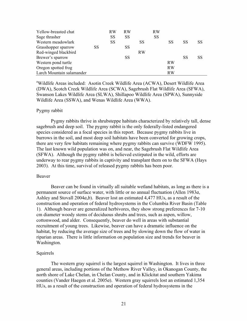
Pygmy rabbit
Pygmy rabbits thrive in shrubsteppe habitats characterized by relatively tall, dense sagebrush and deep soil. The pygmy rabbit is the only federally-listed endangered species considered as a focal species in this report. Because pygmy rabbits live in burrows in the soil, and most deep soil habitats have been converted for growing crops, there are very few habitats remaining where pygmy rabbits can survive (WDFW 1995). The last known wild population was on, and near, the Sagebrush Flat Wildlife Area (SFWA). Although the pygmy rabbit is believed extirpated in the wild, efforts are underway to rear pygmy rabbits in captivity and transplant them on to the SFWA (Hays 2003). At this time, survival of released pygmy rabbits has been poor.
Beaver
Beaver can be found in virtually all suitable wetland habitats, as long as there is a permanent source of surface water, with little or no annual fluctuation (Allen 1983a, Ashley and Stovall 2004a,b). Beaver lost an estimated 4,477 HUs, as a result of the construction and operation of federal hydrosystems in the Columbia River Basin (Table 1). Although beaver are generalized herbivores, they show strong preferences for 7-10 cm diameter woody stems of deciduous shrubs and trees, such as aspen, willow, cottonwood, and alder. Consequently, beaver do well in areas with substantial recruitment of young trees. Likewise, beaver can have a dramatic influence on the habitat, by reducing the average size of trees and by slowing down the flow of water in riparian areas. There is little information on population size and trends for beaver in Washington.
Squirrels
The western gray squirrel is the largest squirrel in Washington. It lives in three general areas, including portions of the Methow River Valley, in Okanogan County, the north shore of Lake Chelan, in Chelan County, and in Klickitat and southern Yakima counties (Vander Haegen et al. 2005a). Western gray squirrels lost an estimated 1,354 HUs, as a result of the construction and operation of federal hydrosystems in the
22
Columbia Basin (Table 1). No population is known to exist on any BPA-funded Wildlife Areas, but there is a possibility that some western gray squirrels may be on or near portions of the Wenas Wildlife Area (WWA). One reason for this possibility is that western portions of the WWA are dominated by Ponderosa pine, mixed with Oregon oak, which is the primary habitat for the western gray squirrel. There is little available information on statewide populations and trends [see Vander Haegen et al. (2004a) for local exception]. In contrast to the gray squirrel, the Washington ground squirrel is closely associated with shrub-steppe habitat, primarily on the SFWA and DWA (Finger et al. 2007). Because of this close association, it is a species of great interest on BPA-funded wildlife areas.
Bighorn sheep
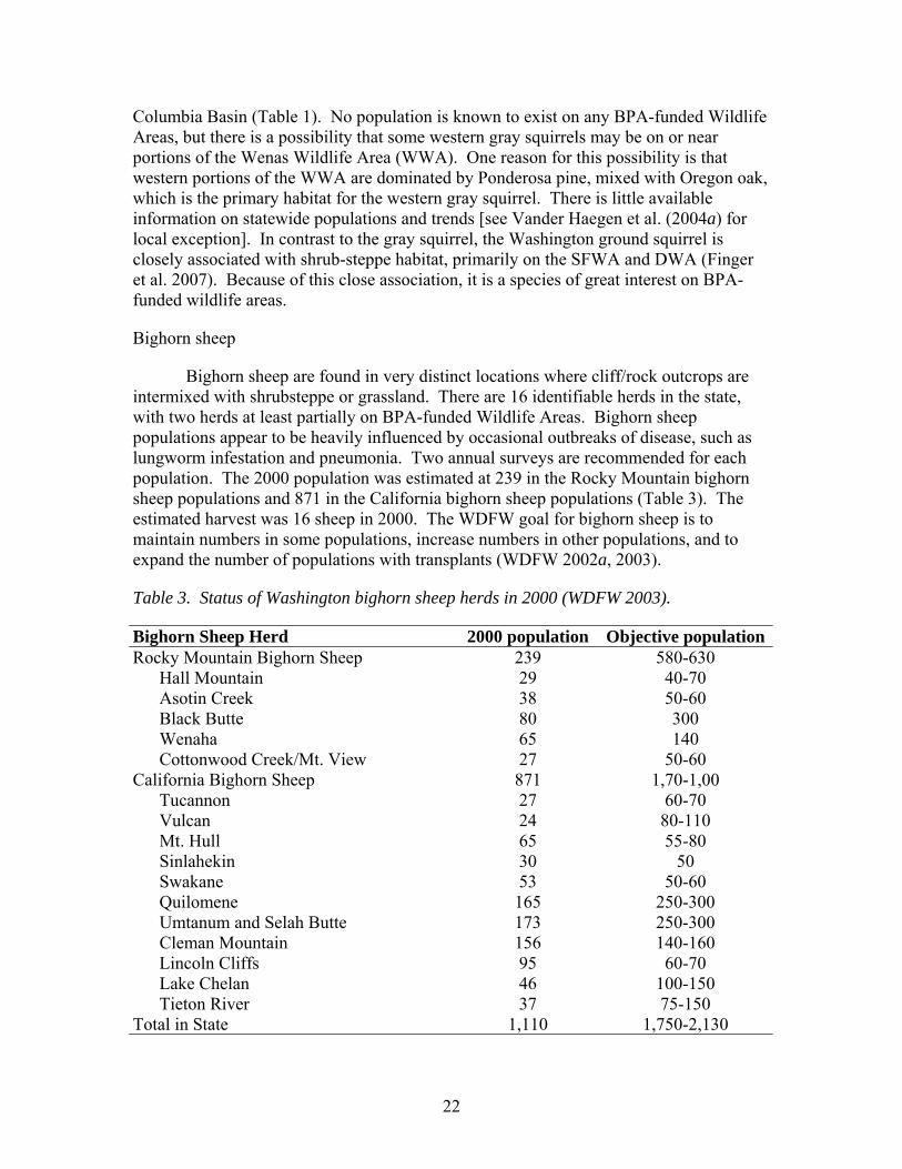
Bighorn sheep are found in very distinct locations where cliff/rock outcrops are intermixed with shrubsteppe or grassland. There are 16 identifiable herds in the state, with two herds at least partially on BPA-funded Wildlife Areas. Bighorn sheep populations appear to be heavily influenced by occasional outbreaks of disease, such as lungworm infestation and pneumonia. Two annual surveys are recommended for each population. The 2000 population was estimated at 239 in the Rocky Mountain bighorn sheep populations and 871 in the California bighorn sheep populations (Table 3). The estimated harvest was 16 sheep in 2000. The WDFW goal for bighorn sheep is to maintain numbers in some populations, increase numbers in other populations, and to expand the number of populations with transplants (WDFW 2002a, 2003).
Table 3. Status of Washington bighorn sheep herds in 2000 (WDFW 2003).
Bighorn Sheep Herd 2000 population Objective populationRocky Mountain Bighorn Sheep 239 580-630 Hall Mountain 29 40-70 Asotin Creek 38 50-60 Black Butte 80 300 Wenaha 65 140 Cottonwood Creek/Mt. View 27 50-60 California Bighorn Sheep 871 1,70-1,00 Tucannon 27 60-70 Vulcan 24 80-110 Mt. Hull 65 55-80 Sinlahekin 30 50 Swakane 53 50-60 Quilomene 165 250-300 Umtanum and Selah Butte 173 250-300 Cleman Mountain 156 140-160 Lincoln Cliffs 95 60-70 Lake Chelan 46 100-150 Tieton River 37 75-150 Total in State 1,110 1,750-2,130
23
Deer
Deer are found throughout the state in almost every habitat. Black-tailed deer are most common on the west side of the Cascade Mountains; mule deer are common in the eastern two thirds; and white-tailed deer are increasingly common in the eastern portions of Washington. Mule deer lost an estimated 40,003 HUs, as a result of the construction and operation of federal hydrosystems in the Columbia River Basin (Table 1). Mule deer populations are believed influenced by severe winter weather and over-harvest. As a consequence, multiple annual surveys are recommended to monitor populations. Although there is no statewide estimate of mule deer populations, the estimated harvest was 11,883 in 2000. The WDFW goal for mule deer is to maintain numbers within limits of landowner tolerance (WDFW 2002a, 2003). WDFW also attempts to maintain a buck:doe ratio of at least 15:100 after the hunting season. In general, mule deer depend on habitats with a substantial layer of shrubs (Ashley and Berger 1999).
Elk
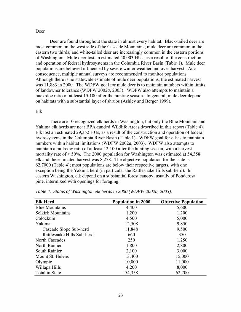
There are 10 recognized elk herds in Washington, but only the Blue Mountain and Yakima elk herds are near BPA-funded Wildlife Areas described in this report (Table 4). Elk lost an estimated 29,352 HUs, as a result of the construction and operation of federal hydrosystems in the Columbia River Basin (Table 1). WDFW goal for elk is to maintain numbers within habitat limitations (WDFW 2002a, 2003). WDFW also attempts to maintain a bull:cow ratio of at least 12:100 after the hunting season, with a harvest mortality rate of < 50%. The 2000 population for Washington was estimated at 54,358 elk and the estimated harvest was 8,278. The objective population for the state is 62,7000 (Table 4); most populations are below their respective targets, with one exception being the Yakima herd (in particular the Rattlesnake Hills sub-herd). In eastern Washington, elk depend on a substantial forest canopy, usually of Ponderosa pine, intermixed with openings for foraging.
Table 4. Status of Washington elk herds in 2000 (WDFW 2002b, 2003).
Elk Herd Population in 2000 Objective Population Blue Mountains 4,400 5,600 Selkirk Mountains 1,200 1,200 Colockum 4,500 5,000 Yakima 12,508 9,850 Cascade Slope Sub-herd 11,848 9,500 Rattlesnake Hills Sub-herd 660 350 North Cascades 250 1,250 North Rainier 1,800 2,800 South Rainier 2,100 3,000 Mount St. Helens 13,400 15,000 Olympic 10,000 11,000 Willapa Hills 4,200 8,000 Total in State 54,358 62,700

24
Mink
The mink is a predatory mammal that lives in semi-aquatic habitats (Allen 1984b). Because the mink has a variable diet, its use of habitat can fluctuate depending on prey availability. Even with the variability, mink are generally associated with the ecotones between habitats that provide cover (usually with structural complexity) and those that provide food.
Sharp-tailed grouse
Sharp-tailed grouse depend on herbaceous-dominated shrubsteppe for nesting and brood-rearing (Schroeder et al. 2000a, Ashley 2006b). They also depend on the deciduous trees and shrubs associated with riparian wetlands for wintering, especially when snow covers the ground. Both of these habitats have been altered and/or have diminished substantially in Washington, which is why the sharp-tailed grouse has declined in both distribution (97% from historical range) and abundance (82% between 1965 and 2008; Fig. 1, see also Schroeder et al. 2000a). The 2008 statewide population was estimated to be 782 and some of the remaining birds were located on SLWA, SCWA, and SFWA, but there is also potential for birds to occur on ACWA. Sharp-tailed grouse lost an estimated 35,545 Habitat Units, as a result of the construction and operation of federal hydrosystems in the Columbia River Basin (Table 1). BPA-funded wildlife areas also have been the focus of recent efforts to augment populations with grouse translocated from other regions.
Fig. 1. Long-term population trends of sharp-tailed grouse in Washington (Schroeder et al. 2000a, with more recent data added).
0
500
1000
1500
2000
2500
3000
3500
4000
4500
1964 1968 1972 1976 1980 1984 1988 1992 1996 2000 2004 2008
Popu
latio
n es
timat
e
25
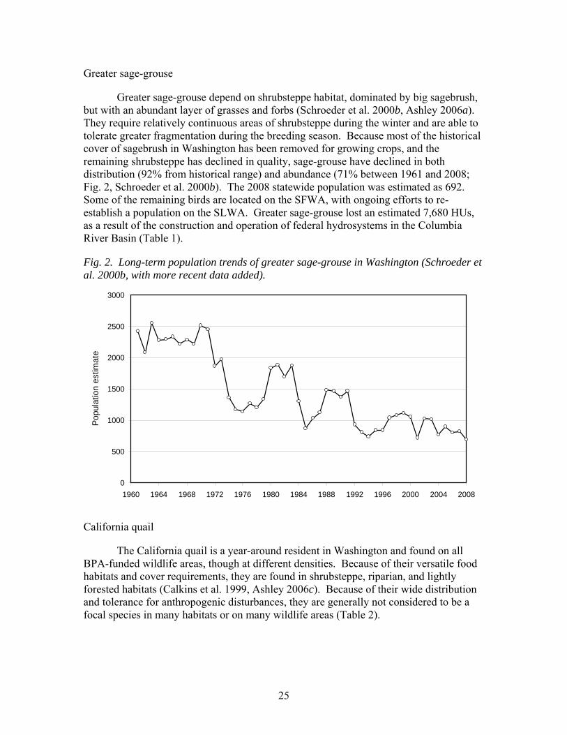
Greater sage-grouse
Greater sage-grouse depend on shrubsteppe habitat, dominated by big sagebrush, but with an abundant layer of grasses and forbs (Schroeder et al. 2000b, Ashley 2006a). They require relatively continuous areas of shrubsteppe during the winter and are able to tolerate greater fragmentation during the breeding season. Because most of the historical cover of sagebrush in Washington has been removed for growing crops, and the remaining shrubsteppe has declined in quality, sage-grouse have declined in both distribution (92% from historical range) and abundance (71% between 1961 and 2008; Fig. 2, Schroeder et al. 2000b). The 2008 statewide population was estimated as 692. Some of the remaining birds are located on the SFWA, with ongoing efforts to re-establish a population on the SLWA. Greater sage-grouse lost an estimated 7,680 HUs, as a result of the construction and operation of federal hydrosystems in the Columbia River Basin (Table 1).
Fig. 2. Long-term population trends of greater sage-grouse in Washington (Schroeder et al. 2000b, with more recent data added).
0
500
1000
1500
2000
2500
3000
1960 1964 1968 1972 1976 1980 1984 1988 1992 1996 2000 2004 2008
Popu
latio
n es
timat
e
California quail
The California quail is a year-around resident in Washington and found on all BPA-funded wildlife areas, though at different densities. Because of their versatile food habitats and cover requirements, they are found in shrubsteppe, riparian, and lightly forested habitats (Calkins et al. 1999, Ashley 2006c). Because of their wide distribution and tolerance for anthropogenic disturbances, they are generally not considered to be a focal species in many habitats or on many wildlife areas (Table 2).
26
Sandhill crane
The sandhill crane is found throughout much of Washington, but primarily during the spring and autumn migrations. Because they are associated with wetlands during the breeding season (Armbruster 1987), and wetlands are not very common on our wildlife areas, they are only considered to be a focal species on the Shillapoo Wildlife Area (Table 2).
Great blue heron
The great blue heron is found in suitable habitat throughout most of Washington. Great blue herons lost an estimated 7,913 HUs, as a result of the construction and operation of federal hydrosystems in the Columbia River Basin (Table 1). Trends in portions of northwestern North America appear to be negative, but the 1966-2003 trends in the Columbia River Basin were not significant, based on Breeding Bird Survey (BBS) data (P = 0.880; Sauer et al. 2004). Great blue herons have a close association with wetlands, where they feed on a large diversity of aquatic and marine animals found in shallow water (Short and Cooper 1985, Quinn and Milner 1999). In addition, great blue herons tend to aggregate during the breeding season, often nesting in colonies.
Canada goose
The Canada goose is an extremely important game bird in North America and in Washington. It is considered to be a focal species only on the Shillapoo Wildlife Area, primarily because of its dominant wetlands. Even so, the Canada goose is associated with other wildlife areas, but largely during migration and then only in the relatively restricted wetland habitats (Martin et al. 1987).
Mallard
The mallard is one of the most important game birds in North America and it is the most abundant duck species in Washington, where it is widely distributed. Mallards depend on riparian wetland or grassland habitat, near water, for nesting (Martin et al. 1987). Wide distribution of nesting habitat tends to improve nest success. Mallards lost an estimated 27,190 HUs, as a result of the construction and operation of federal hydrosystems in the Columbia River Basin (Table 1); a substantial amount of this lost habitat was in the Yakima Subbasin (YS), where surveys started in the 1940s (NPPC 2004g). Documented declines were substantial, particularly in the area near the Sunnyside Wildlife Area (SWA) and WWA, where the mallard is a focal species. Trends in North America appear to be a function of which dates are surveyed (Johnson and Shaffer 1987), but were not significant for the 1966 to 2003 period (P = 0.761, Sauer et al. 2004). Harvest data also illustrate the importance of mallards in the YS; Yakima County had the highest duck harvest in 2003 (28,327 mallards) (WDFW 2004a).
Bald eagle
Bald eagles are widely distributed in Washington, but primarily associated with aquatic habitats (Martin et al. 1987). Consequently, the Shillapoo Wildlife Area is the
27
only area that considers them a focal species. Habitat management primarily focuses on reducing the use of lead shot for waterfowl hunting, retention of suitable trees for nesting and roosting, and reduction of disturbance near nest sites, particularly during the breeding season (Martin et al. 1987, Buehler 2000). The bald eagle lost an estimated 14,702 HUs, as a result of the construction and operation of federal hydrosystems in the Columbia River Basin (Table 1).
Golden eagle
The golden eagle is sparsely distributed, but present on most wildlife areas in eastern Washington. One reason why golden eagles are uncommon is that they have large home ranges and depend primarily on cliff habitats for placement of nest sites (McCall and Musser 2000). Their foraging habitat is variable, but primarily in shrubsteppe, grassland, and open Ponderosa pine, all common on wildlife areas in eastern Washington.
Flammulated owl
Flammulated owls are found in a relatively narrow band of Ponderosa pine/Douglas fir forest. They appear to depend on old trees, open forests, and snags. Because of their relatively small distribution and infrequent sightings, there is not enough BBS data to illustrate changes in their range-wide distribution, or to examine the significance of long-term changes in populations (Sauer et al. 2004). Even though their population status is unknown, their lack of abundance and narrow habitat preferences have resulted in their use as a focal species on multiple wildlife areas.
Band-tailed pigeon
The band-tailed pigeon is primarily associated with coniferous forests in western Washington (Lewis et al. 2003). The only BPA-funded wildlife area in the range of the band-tailed pigeon is the Shillapoo Wildlife Area. Although the band-tailed pigeon is considered a game birds, the season has been closed in Washington since 1991. The primary management considerations include protection of mineral springs that are required during the breeding and brood-rearing seasons and protection of their coniferous habitat.
Red-eyed vireo
The red-eyed vireo appears to have a very patchy distribution in the state of Washington, associated mostly with black cottonwood in riparian corridors. There was not enough data to statistically examine long-term population trends in the Columbia River Basin, but the BBS range map appeared to suggest that there were long-term declines, particularly in Washington (Sauer et al. 2004).
Black-capped chickadee
The black-capped chickadee is found in suitable habitat throughout most of Washington. Within the wildlife area system, these suitable habitats largely include the
28
riparian areas, particular woodland. The black-capped chickadee is a cavity nester and an insectivorous gleaner (Schroeder 1983a). Chickadees lost an estimated 6,631 HUs a result of the construction and operation of federal hydrosystems in the Columbia River Basin (Table 1).
Pygmy nuthatch
The pygmy nuthatch is closely associated with dry Ponderosa pine forests; even there, nuthatch distribution is patchy. They appear to select areas with very old trees and abundant snags. There was no indication of any long-term population trend (P = 0.622; Sauer et al. 2004), but the BBS range map appeared to suggest that there were long-term increases, particularly in Washington (Sauer et al. 2004).
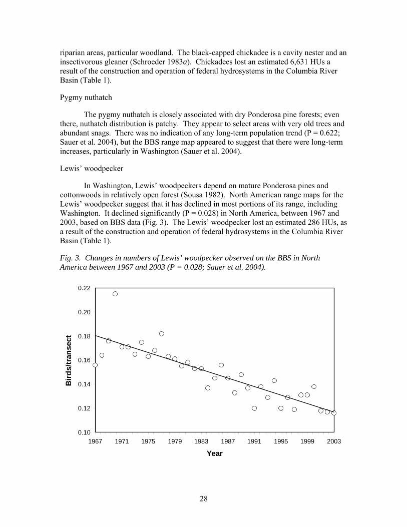
Lewis’ woodpecker
In Washington, Lewis’ woodpeckers depend on mature Ponderosa pines and cottonwoods in relatively open forest (Sousa 1982). North American range maps for the Lewis’ woodpecker suggest that it has declined in most portions of its range, including Washington. It declined significantly (P = 0.028) in North America, between 1967 and 2003, based on BBS data (Fig. 3). The Lewis’ woodpecker lost an estimated 286 HUs, as a result of the construction and operation of federal hydrosystems in the Columbia River Basin (Table 1).
Fig. 3. Changes in numbers of Lewis’ woodpecker observed on the BBS in North America between 1967 and 2003 (P = 0.028; Sauer et al. 2004).
0.10
0.12
0.14
0.16
0.18
0.20
0.22
1967 1971 1975 1979 1983 1987 1991 1995 1999 2003
Year
Bird
s/tr
anse
ct
29
Downy woodpecker
The downy woodpecker is widespread, but considered a focal species only in the riparian habitats of the Sunnyside Wildlife Area. The downy woodpecker is an insectivorous cavity nester that is dependent on woodland habitats for selection of both its nesting and foraging sites (Schroeder 1982a). Although deciduous trees seem to be preferred, downy woodpeckers may also use coniferous habitats, often in situations that are relatively open. The Downy woodpecker lost an estimated 742 HUs, as a result of the construction and operation of federal hydrosystems in the Columbia River Basin (Table 1).
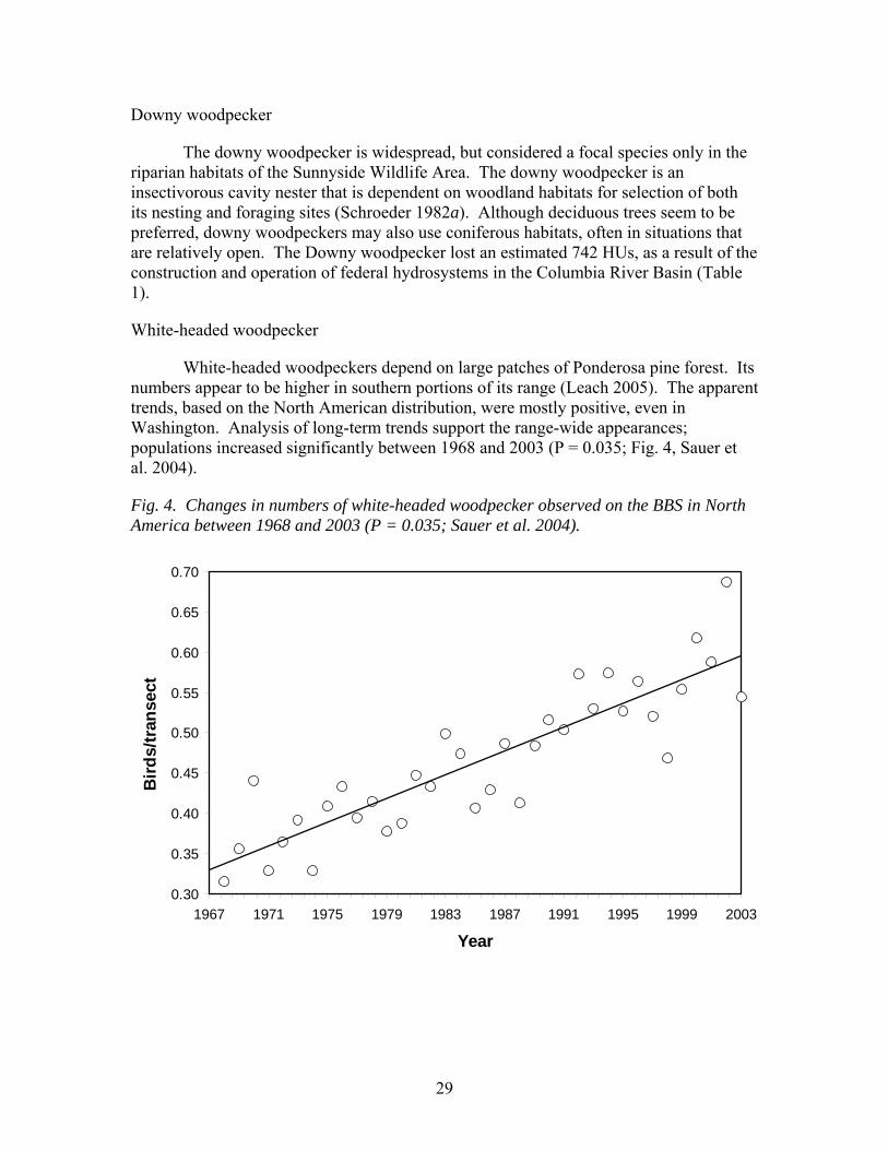
White-headed woodpecker
White-headed woodpeckers depend on large patches of Ponderosa pine forest. Its numbers appear to be higher in southern portions of its range (Leach 2005). The apparent trends, based on the North American distribution, were mostly positive, even in Washington. Analysis of long-term trends support the range-wide appearances; populations increased significantly between 1968 and 2003 (P = 0.035; Fig. 4, Sauer et al. 2004).
Fig. 4. Changes in numbers of white-headed woodpecker observed on the BBS in North America between 1968 and 2003 (P = 0.035; Sauer et al. 2004).
0.30
0.35
0.40
0.45
0.50
0.55
0.60
0.65
0.70
1967 1971 1975 1979 1983 1987 1991 1995 1999 2003
Year
Bird
s/tr
anse
ct
30
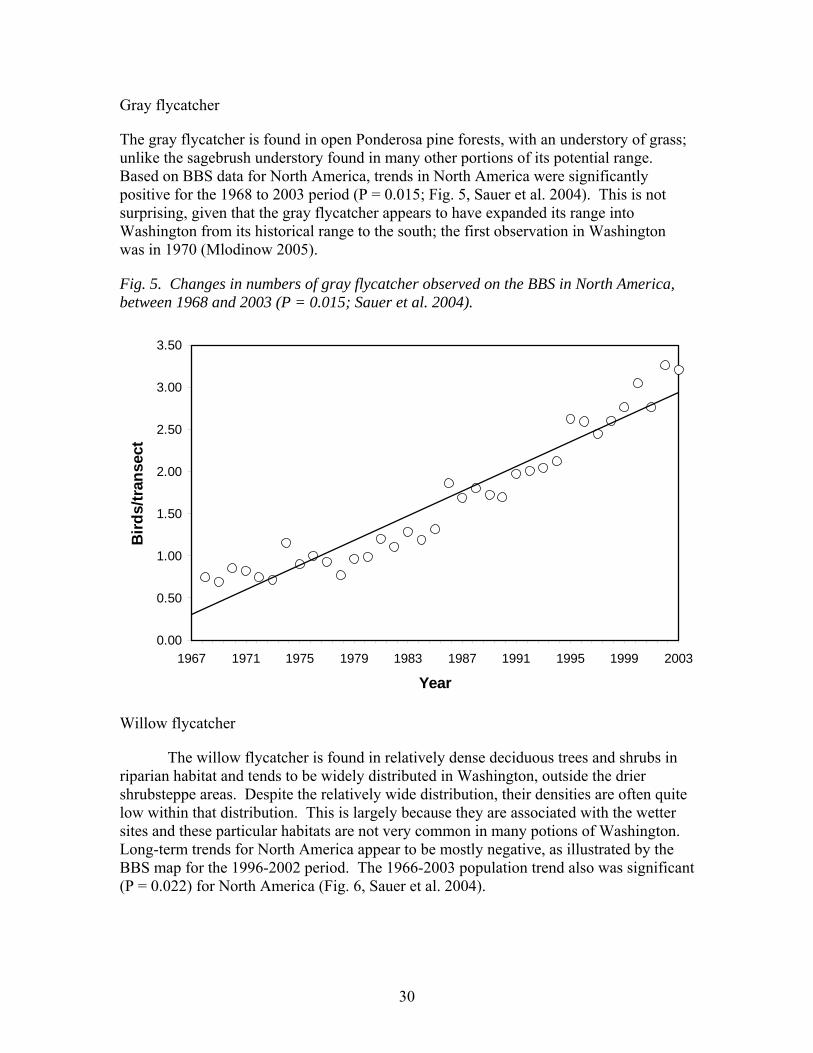
Gray flycatcher
The gray flycatcher is found in open Ponderosa pine forests, with an understory of grass; unlike the sagebrush understory found in many other portions of its potential range. Based on BBS data for North America, trends in North America were significantly positive for the 1968 to 2003 period (P = 0.015; Fig. 5, Sauer et al. 2004). This is not surprising, given that the gray flycatcher appears to have expanded its range into Washington from its historical range to the south; the first observation in Washington was in 1970 (Mlodinow 2005).
Fig. 5. Changes in numbers of gray flycatcher observed on the BBS in North America, between 1968 and 2003 (P = 0.015; Sauer et al. 2004).
0.00
0.50
1.00
1.50
2.00
2.50
3.00
3.50
1967 1971 1975 1979 1983 1987 1991 1995 1999 2003
Year
Bird
s/tr
anse
ct
Willow flycatcher
The willow flycatcher is found in relatively dense deciduous trees and shrubs in riparian habitat and tends to be widely distributed in Washington, outside the drier shrubsteppe areas. Despite the relatively wide distribution, their densities are often quite low within that distribution. This is largely because they are associated with the wetter sites and these particular habitats are not very common in many potions of Washington. Long-term trends for North America appear to be mostly negative, as illustrated by the BBS map for the 1996-2002 period. The 1966-2003 population trend also was significant (P = 0.022) for North America (Fig. 6, Sauer et al. 2004).

31
Fig. 6. Changes in numbers of willow flycatcher observed on the BBS in the Columbia Basin, between 1966 and 2003 (P = 0.022; Sauer et al. 2004).
1.00
1.05
1.10
1.15
1.20
1.25
1.30
1.35
1.40
1.45
1966 1970 1974 1978 1982 1986 1990 1994 1998 2002
Year
Bird
s/tr
anse
ct
Yellow warbler
The yellow warbler is common and widespread in suitable habitat, primarily deciduous shrubs/trees in riparian areas (Schroeder 1982d). The yellow warbler population trends in the Columbia River Basin have been insignificant (P = 0.819) and the North American range map illustrates regional variation in long-term trends (Sauer et al. 2004). Nevertheless, the North American map suggests that yellow warbler numbers have declined in much of the Columbia River Basin. Yellow warblers lost an estimated 6,519 HUs, as a result of the construction and operation of federal hydrosystems in the Columbia River Basin (Table 1).
Yellow-breasted chat
The yellow-breasted chat nests in thick and diverse riparian wetland habitats. There have been no indications of a long-term population change in the Columbia River Basin (P = 0.893; Sauer et al. 2004). The North American range map suggests that the yellow-breasted chat actually may have increased in portions of the Columbia River Basin, including Washington (Sauer et al. 2004).
Sage thrasher
The sage thrasher depends almost entirely on sagebrush; and so, it is rarely found far from sagebrush-dominated shrubsteppe. They appear to select areas with relatively
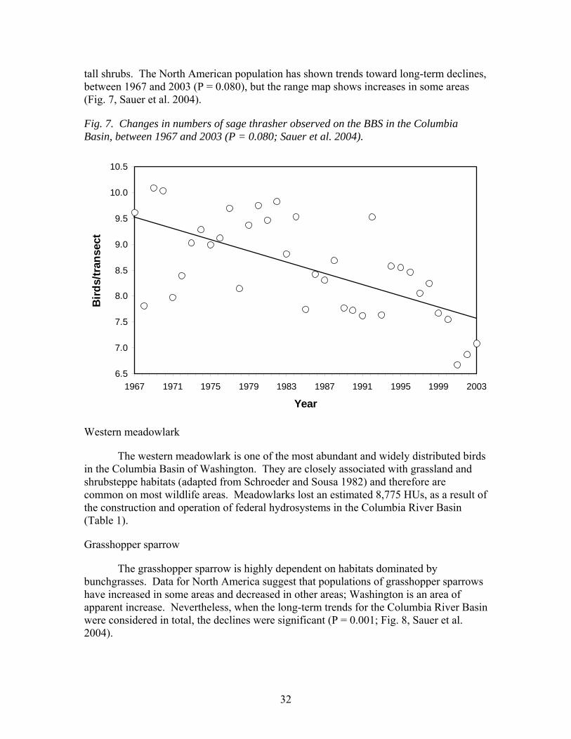
32
tall shrubs. The North American population has shown trends toward long-term declines, between 1967 and 2003 (P = 0.080), but the range map shows increases in some areas (Fig. 7, Sauer et al. 2004).
Fig. 7. Changes in numbers of sage thrasher observed on the BBS in the Columbia Basin, between 1967 and 2003 (P = 0.080; Sauer et al. 2004).
6.5
7.0
7.5
8.0
8.5
9.0
9.5
10.0
10.5
1967 1971 1975 1979 1983 1987 1991 1995 1999 2003
Year
Bird
s/tr
anse
ct
Western meadowlark
The western meadowlark is one of the most abundant and widely distributed birds in the Columbia Basin of Washington. They are closely associated with grassland and shrubsteppe habitats (adapted from Schroeder and Sousa 1982) and therefore are common on most wildlife areas. Meadowlarks lost an estimated 8,775 HUs, as a result of the construction and operation of federal hydrosystems in the Columbia River Basin (Table 1).
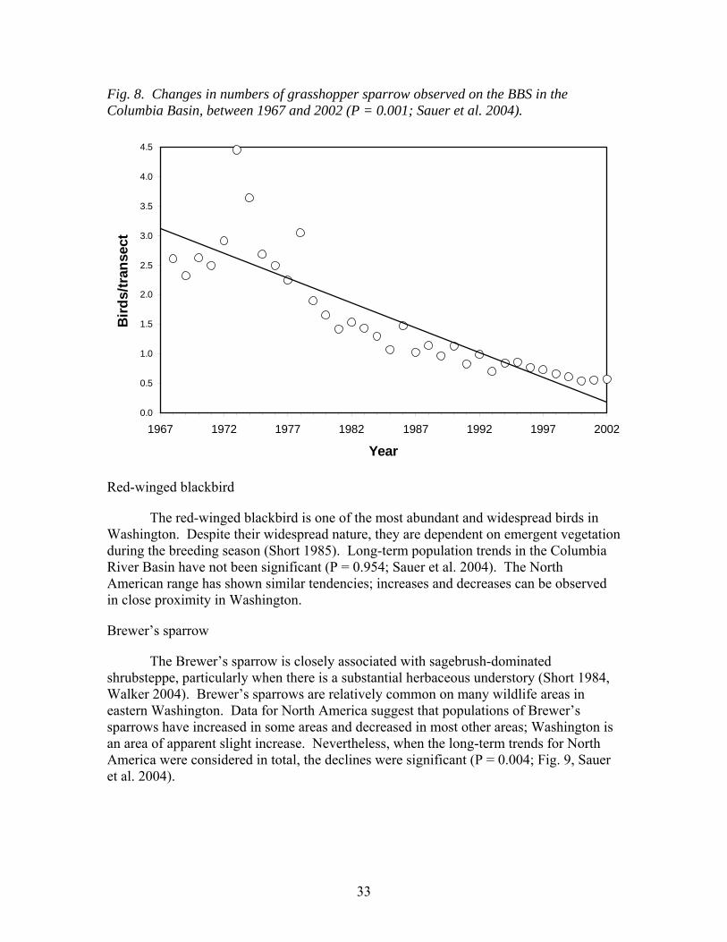
Grasshopper sparrow
The grasshopper sparrow is highly dependent on habitats dominated by bunchgrasses. Data for North America suggest that populations of grasshopper sparrows have increased in some areas and decreased in other areas; Washington is an area of apparent increase. Nevertheless, when the long-term trends for the Columbia River Basin were considered in total, the declines were significant (P = 0.001; Fig. 8, Sauer et al. 2004).
33
Fig. 8. Changes in numbers of grasshopper sparrow observed on the BBS in the Columbia Basin, between 1967 and 2002 (P = 0.001; Sauer et al. 2004).
0.0
0.5
1.0
1.5
2.0
2.5
3.0
3.5
4.0
4.5
1967 1972 1977 1982 1987 1992 1997 2002
Year
Bird
s/tr
anse
ct
Red-winged blackbird
The red-winged blackbird is one of the most abundant and widespread birds in Washington. Despite their widespread nature, they are dependent on emergent vegetation during the breeding season (Short 1985). Long-term population trends in the Columbia River Basin have not been significant (P = 0.954; Sauer et al. 2004). The North American range has shown similar tendencies; increases and decreases can be observed in close proximity in Washington.
Brewer’s sparrow
The Brewer’s sparrow is closely associated with sagebrush-dominated shrubsteppe, particularly when there is a substantial herbaceous understory (Short 1984, Walker 2004). Brewer’s sparrows are relatively common on many wildlife areas in eastern Washington. Data for North America suggest that populations of Brewer’s sparrows have increased in some areas and decreased in most other areas; Washington is an area of apparent slight increase. Nevertheless, when the long-term trends for North America were considered in total, the declines were significant (P = 0.004; Fig. 9, Sauer et al. 2004).
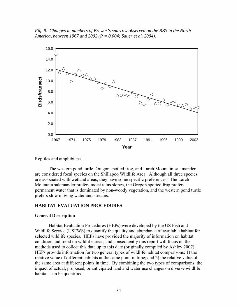
34
Fig. 9. Changes in numbers of Brewer’s sparrow observed on the BBS in the North America, between 1967 and 2002 (P = 0.004; Sauer et al. 2004).
0.0
2.0
4.0
6.0
8.0
10.0
12.0
14.0
16.0
1967 1971 1975 1979 1983 1987 1991 1995 1999 2003
Year
Bird
s/tr
anse
ct
Reptiles and amphibians
The western pond turtle, Oregon spotted frog, and Larch Mountain salamander are considered focal species on the Shillapoo Wildlife Area. Although all three species are associated with wetland areas, they have some specific preferences. The Larch Mountain salamander prefers moist talus slopes, the Oregon spotted frog prefers permanent water that is dominated by non-woody vegetation, and the western pond turtle prefers slow moving water and streams.
HABITAT EVALUATION PROCEDURES
General Description
Habitat Evaluation Procedures (HEPs) were developed by the US Fish and Wildlife Service (USFWS) to quantify the quality and abundance of available habitat for selected wildlife species. HEPs have provided the majority of information on habitat condition and trend on wildlife areas, and consequently this report will focus on the methods used to collect this data up to this date (originally compiled by Ashley 2007). HEPs provide information for two general types of wildlife habitat comparisons: 1) the relative value of different habitats at the same point in time; and 2) the relative value of the same area at different points in time. By combining the two types of comparisons, the impact of actual, proposed, or anticipated land and water use changes on diverse wildlife habitats can be quantified.
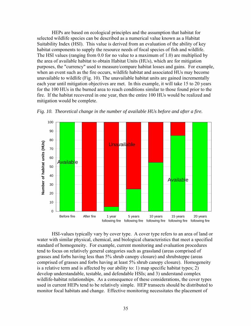
35
HEPs are based on ecological principles and the assumption that habitat for selected wildlife species can be described as a numerical value known as a Habitat Suitability Index (HSI). This value is derived from an evaluation of the ability of key habitat components to supply the resource needs of focal species of fish and wildlife. The HSI values (ranging from 0.0 for no value to a maximum of 1.0) are multiplied by the area of available habitat to obtain Habitat Units (HUs), which are for mitigation purposes, the "currency" used to measure/compare habitat losses and gains. For example, when an event such as the fire occurs, wildlife habitat and associated HUs may become unavailable to wildlife (Fig. 10). The unavailable habitat units are gained incrementally each year until mitigation objectives are met. In this example, it will take 15 to 20 years for the 100 HUs in the burned area to reach conditions similar to those found prior to the fire. If the habitat recovered in one year, then the entire 100 HUs would be realized and mitigation would be complete.
Fig. 10. Theoretical change in the number of available HUs before and after a fire.
Available
Unavailable
Available
0
10
20
30
40
50
60
70
80
90
100
Before fire After fire 1 yearfollowing fire
5 yearsfollowing fire
10 yearsfollowing fire
15 yearsfollowing fire
20 yearsfollowing fire
Num
ber
of h
abita
t uni
ts (H
Us)
HSI-values typically vary by cover type. A cover type refers to an area of land or water with similar physical, chemical, and biological characteristics that meet a specified standard of homogeneity. For example, current monitoring and evaluation procedures tend to focus on relatively general categories such as grassland (areas comprised of grasses and forbs having less than 5% shrub canopy closure) and shrubsteppe (areas comprised of grasses and forbs having at least 5% shrub canopy closure). Homogeneity is a relative term and is affected by our ability to: 1) map specific habitat types; 2) develop understandable, testable, and defendable HSIs; and 3) understand complex wildlife-habitat relationships. As a consequence of these considerations, the cover types used in current HEPs tend to be relatively simple. HEP transects should be distributed to monitor focal habitats and change. Effective monitoring necessitates the placement of
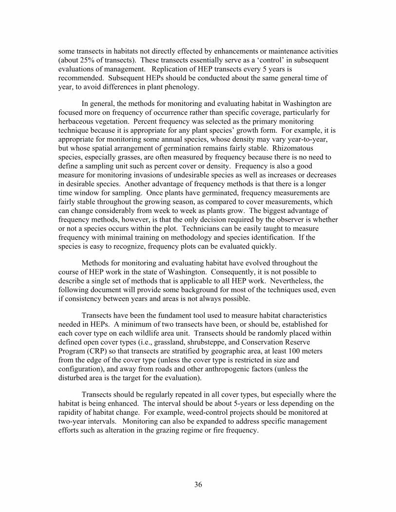
36
some transects in habitats not directly effected by enhancements or maintenance activities (about 25% of transects). These transects essentially serve as a ‘control’ in subsequent evaluations of management. Replication of HEP transects every 5 years is recommended. Subsequent HEPs should be conducted about the same general time of year, to avoid differences in plant phenology.
In general, the methods for monitoring and evaluating habitat in Washington are focused more on frequency of occurrence rather than specific coverage, particularly for herbaceous vegetation. Percent frequency was selected as the primary monitoring technique because it is appropriate for any plant species’ growth form. For example, it is appropriate for monitoring some annual species, whose density may vary year-to-year, but whose spatial arrangement of germination remains fairly stable. Rhizomatous species, especially grasses, are often measured by frequency because there is no need to define a sampling unit such as percent cover or density. Frequency is also a good measure for monitoring invasions of undesirable species as well as increases or decreases in desirable species. Another advantage of frequency methods is that there is a longer time window for sampling. Once plants have germinated, frequency measurements are fairly stable throughout the growing season, as compared to cover measurements, which can change considerably from week to week as plants grow. The biggest advantage of frequency methods, however, is that the only decision required by the observer is whether or not a species occurs within the plot. Technicians can be easily taught to measure frequency with minimal training on methodology and species identification. If the species is easy to recognize, frequency plots can be evaluated quickly.
Methods for monitoring and evaluating habitat have evolved throughout the course of HEP work in the state of Washington. Consequently, it is not possible to describe a single set of methods that is applicable to all HEP work. Nevertheless, the following document will provide some background for most of the techniques used, even if consistency between years and areas is not always possible.
Transects have been the fundament tool used to measure habitat characteristics needed in HEPs. A minimum of two transects have been, or should be, established for each cover type on each wildlife area unit. Transects should be randomly placed within defined open cover types (i.e., grassland, shrubsteppe, and Conservation Reserve Program (CRP) so that transects are stratified by geographic area, at least 100 meters from the edge of the cover type (unless the cover type is restricted in size and configuration), and away from roads and other anthropogenic factors (unless the disturbed area is the target for the evaluation).
Transects should be regularly repeated in all cover types, but especially where the habitat is being enhanced. The interval should be about 5-years or less depending on the rapidity of habitat change. For example, weed-control projects should be monitored at two-year intervals. Monitoring can also be expanded to address specific management efforts such as alteration in the grazing regime or fire frequency.
37
Methods for Open Habitats
Two types of transects configurations are used in open habitats. In one technique, 100-meter baseline transects are oriented along a random azimuth. An alternate azimuth (random or varied by 45 degrees from first azimuth) is used if the first baseline transect exits the cover type. Ten 30-meter transects are anchored on the baseline transect and oriented at a 90 degree angle (perpendicular) to the baseline transect. The location of the first perpendicular transect is selected at random location between 0-10 meters from the start point on the baseline transect. The following perpendicular transects are placed systematically at ten-meter intervals on the baseline transect. For example, if the first perpendicular transect is positioned at the 5-meter mark, the second transect is placed at the 15-meter mark, the third at the 25-meter, and so on until 10 perpendicular transects are established (Fig. 11).
Fig. 11. Layout of baseline and perpendicular transects for HEP work.
Baseline transect – 100 m
Perp
endi
cula
r tra
nsec
ts –
30 m
10 m
Baseline transect – 100 m
Perp
endi
cula
r tra
nsec
ts –
30 m
10 m
In the second type of transect configuration, the baseline transect is used as the primary data-collection transect with no perpendicular transects. The techniques are generally similar, except that the baseline transect is longer in the second technique and the distances between data collection points varies. In addition, with the second technique, the transect direction is altered every 100 meters (or 300 feet depending on the type of tape measure used), or if the cover type changes. In situations where a new azimuth is needed, either a random direction is chosen, or a 45-degree turn is used and the ‘right or left’ decision is determined with the flip of a coin. Regardless of the transect configuration used, transect start, end, and turn points are permanently marked with a 36-centimeter (14-inch) long 0.6-centimeter (¼-inch) rebar stakes painted fluorescent orange or red.
Start, end, and turn points on the baseline transects are determined with GPS equipment. Other relevant information, including observers, date, and azimuths (controlled for declination) are also be recorded. At least one photo is taken at the start point on each baseline transect. The camera is positioned one meter above the ground (use 1-m cover board or similar device for camera rest). The photo includes a 1.5-meter cover board (1.5 m X 0.1 m rectangle with alternating white and red bands at 1-dm

38
intervals) 10-meters in front of the camera, as well as the transect photo board (relevant information for transect identification). The photo is taken from the start point of the baseline transect and facing the transect direction. The camera type, aperture, distance and azimuth to cover board, cover board dimensions, date, time of day, transect/location identification, GPS coordinates, and photographer are recorded. Additional photos are used to document the habitat, but basic information such as date, location, and direction is critical.
Herbaceous vegetation (forbs, grasses, and noxious weeds), biological crusts, bare ground, and rock are measured with the aid of microplots. Microplots are positioned systematically at 3-meter intervals along each perpendicular transect from a random start point (Fig. 12) or at intervals of 6.10 meters (20 feet) or 7.62 meters (25 feet) on the baseline transect. The placement of microplots on the perpendicular transects is determined by selecting a random number between 0 and 3 (the first data collection point for the perpendicular transect). Starting at the first data collection point, place the microplots at 3-meter intervals along the perpendicular transect until 10 microplot measurements are taken. For example, if the first data point is located at 2 meters on the perpendicular transect, the second data point is at 5 meters, the third is at 8 meters, and so forth. The long axis of the microplot (if there is a long axis) is placed perpendicular to the transect azimuth with the microplot edge on the line and the corner at the appropriate transect point (Fig. 12).
Fig. 12. Layout of microplots on perpendicular transects for HEP work.
Microplots – spaced at 3-m intervals on perpendicular transect
Baseline transect
Microplots – spaced at 3-m intervals on perpendicular transect
Baseline transect
Herbaceous vegetation frequency, abundance, and density are collected using the microplots. Microplots vary in size; 0.04-meters2 (20 cm X 20 cm), 0.1-meters2 (31.6 cm X 31.6 cm), 0.16-meters2 (40 cm X 40 cm), and 0.5-meters2 (50 cm X 100 cm). Regardless of the type of microplot used, it is critical that its dimensions and characteristics be recorded, since the frequency of occurrence of many species will be affected by the size of the microplot. In general, species have a greater frequency of occurrence in larger microplots. The 0.5-meter2 microplot is usually used in shrublands and is divided into equal 0.1-meter2 rectangles (10 cm X 50 cm rectangles) to facilitate collection of abundance and percent cover data (Fig. 13). The 0.16-meter2 microplot is nested within a small 10 cm X 10 cm area (0.01-m2) and a medium sized 20 cm X 20 cm area (0.04-m2) that includes the previous small 0.01-meter2 area. The 0.1-meter2 microplot is usually used in grasslands and is nested within five 0.01-meter2 rectangles and a larger 0.05-meter2 rectangle (Fig. 14).
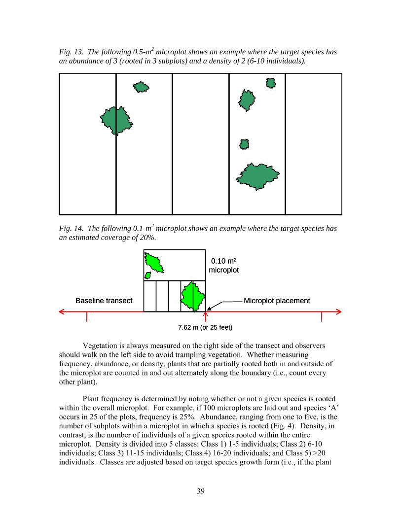
39
Fig. 13. The following 0.5-m2 microplot shows an example where the target species has an abundance of 3 (rooted in 3 subplots) and a density of 2 (6-10 individuals).
Fig. 14. The following 0.1-m2 microplot shows an example where the target species has an estimated coverage of 20%.
7.62 m (or 25 feet)
Baseline transect Microplot placement
0.10 m2
microplot
7.62 m (or 25 feet)
Baseline transect Microplot placement
0.10 m2
microplot
Vegetation is always measured on the right side of the transect and observers should walk on the left side to avoid trampling vegetation. Whether measuring frequency, abundance, or density, plants that are partially rooted both in and outside of the microplot are counted in and out alternately along the boundary (i.e., count every other plant).
Plant frequency is determined by noting whether or not a given species is rooted within the overall microplot. For example, if 100 microplots are laid out and species ‘A’ occurs in 25 of the plots, frequency is 25%. Abundance, ranging from one to five, is the number of subplots within a microplot in which a species is rooted (Fig. 4). Density, in contrast, is the number of individuals of a given species rooted within the entire microplot. Density is divided into 5 classes: Class 1) 1-5 individuals; Class 2) 6-10 individuals; Class 3) 11-15 individuals; Class 4) 16-20 individuals; and Class 5) >20 individuals. Classes are adjusted based on target species growth form (i.e., if the plant
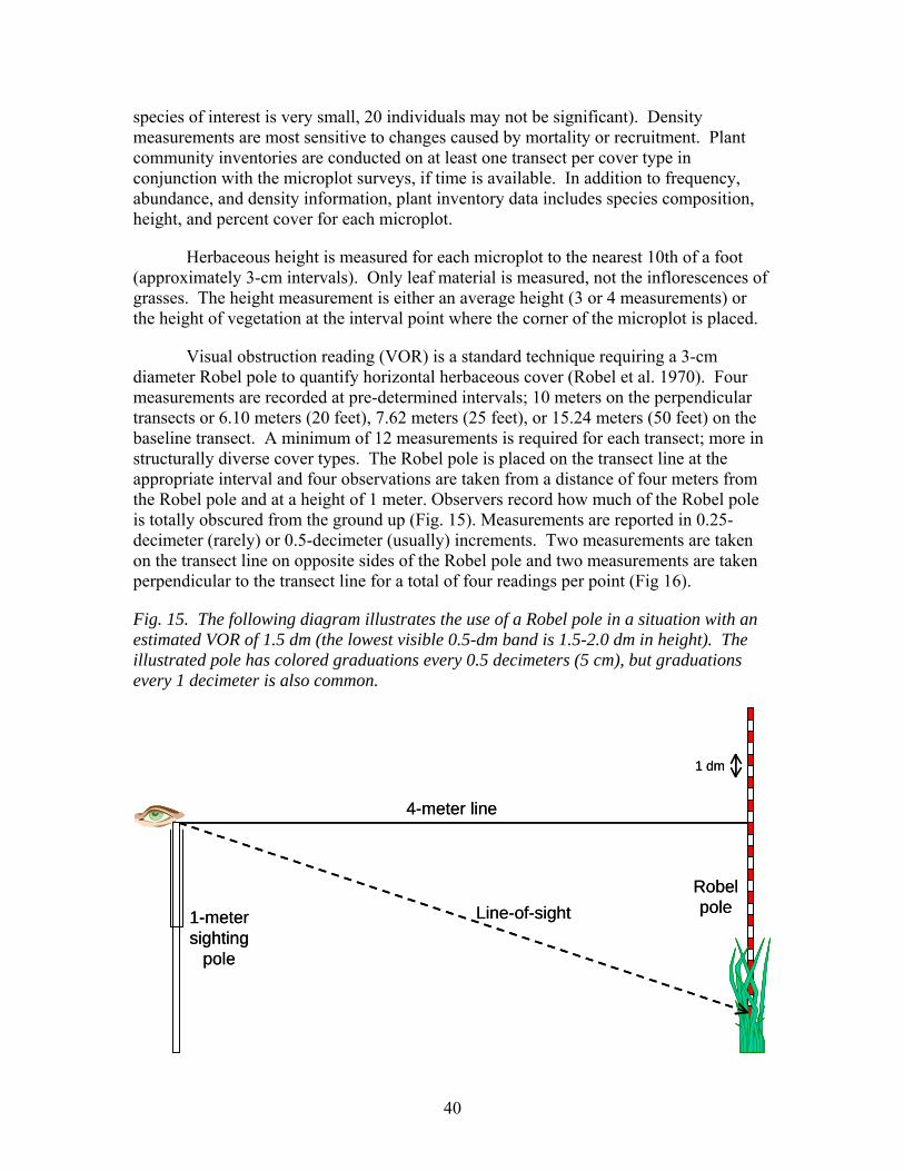
40
species of interest is very small, 20 individuals may not be significant). Density measurements are most sensitive to changes caused by mortality or recruitment. Plant community inventories are conducted on at least one transect per cover type in conjunction with the microplot surveys, if time is available. In addition to frequency, abundance, and density information, plant inventory data includes species composition, height, and percent cover for each microplot.
Herbaceous height is measured for each microplot to the nearest 10th of a foot (approximately 3-cm intervals). Only leaf material is measured, not the inflorescences of grasses. The height measurement is either an average height (3 or 4 measurements) or the height of vegetation at the interval point where the corner of the microplot is placed.
Visual obstruction reading (VOR) is a standard technique requiring a 3-cm diameter Robel pole to quantify horizontal herbaceous cover (Robel et al. 1970). Four measurements are recorded at pre-determined intervals; 10 meters on the perpendicular transects or 6.10 meters (20 feet), 7.62 meters (25 feet), or 15.24 meters (50 feet) on the baseline transect. A minimum of 12 measurements is required for each transect; more in structurally diverse cover types. The Robel pole is placed on the transect line at the appropriate interval and four observations are taken from a distance of four meters from the Robel pole and at a height of 1 meter. Observers record how much of the Robel pole is totally obscured from the ground up (Fig. 15). Measurements are reported in 0.25-decimeter (rarely) or 0.5-decimeter (usually) increments. Two measurements are taken on the transect line on opposite sides of the Robel pole and two measurements are taken perpendicular to the transect line for a total of four readings per point (Fig 16).
Fig. 15. The following diagram illustrates the use of a Robel pole in a situation with an estimated VOR of 1.5 dm (the lowest visible 0.5-dm band is 1.5-2.0 dm in height). The illustrated pole has colored graduations every 0.5 decimeters (5 cm), but graduations every 1 decimeter is also common.
4-meter line
1-meter sighting
pole
Line-of-sightRobel pole
1 dm
4-meter line
1-meter sighting
pole
Line-of-sightRobel pole
1 dm
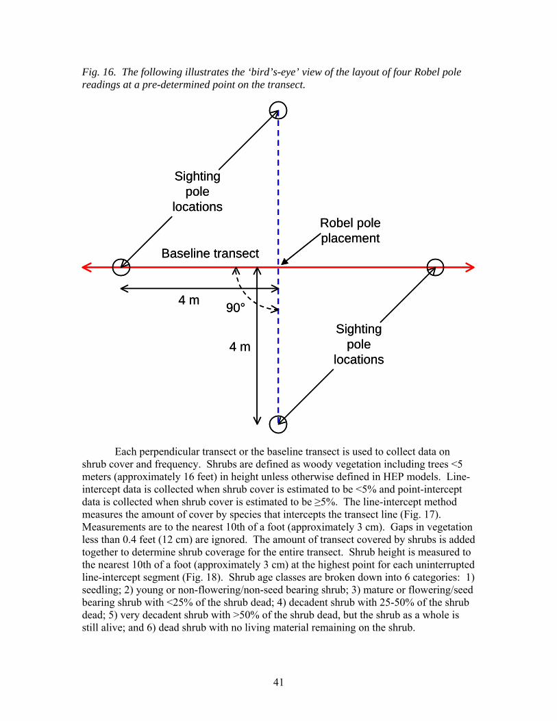
41
Fig. 16. The following illustrates the ‘bird’s-eye’ view of the layout of four Robel pole readings at a pre-determined point on the transect.
Baseline transect
Robel pole placement
Sighting pole
locations
Sighting pole
locations
4 m
4 m
90°
Baseline transect
Robel pole placement
Sighting pole
locations
Sighting pole
locations
4 m
4 m
90°
Each perpendicular transect or the baseline transect is used to collect data on shrub cover and frequency. Shrubs are defined as woody vegetation including trees <5 meters (approximately 16 feet) in height unless otherwise defined in HEP models. Line-intercept data is collected when shrub cover is estimated to be <5% and point-intercept data is collected when shrub cover is estimated to be ≥5%. The line-intercept method measures the amount of cover by species that intercepts the transect line (Fig. 17). Measurements are to the nearest 10th of a foot (approximately 3 cm). Gaps in vegetation less than 0.4 feet (12 cm) are ignored. The amount of transect covered by shrubs is added together to determine shrub coverage for the entire transect. Shrub height is measured to the nearest 10th of a foot (approximately 3 cm) at the highest point for each uninterrupted line-intercept segment (Fig. 18). Shrub age classes are broken down into 6 categories: 1) seedling; 2) young or non-flowering/non-seed bearing shrub; 3) mature or flowering/seed bearing shrub with <25% of the shrub dead; 4) decadent shrub with 25-50% of the shrub dead; 5) very decadent shrub with >50% of the shrub dead, but the shrub as a whole is still alive; and 6) dead shrub with no living material remaining on the shrub.
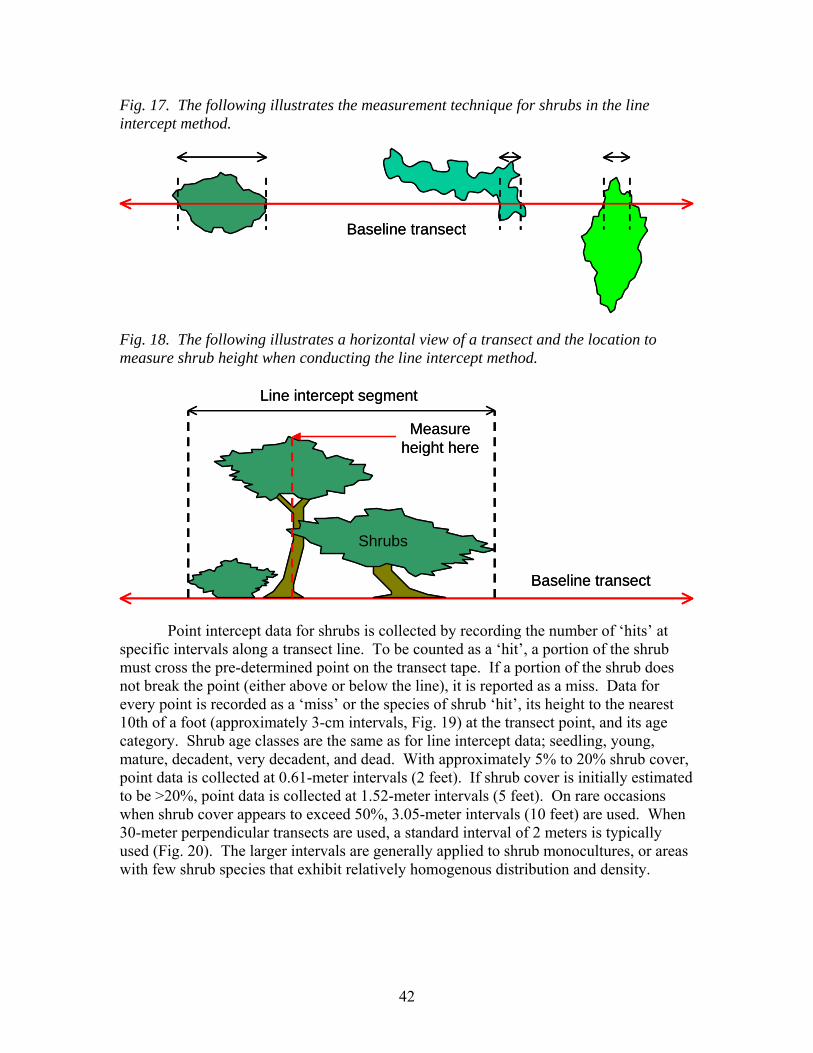
42
Fig. 17. The following illustrates the measurement technique for shrubs in the line intercept method.
Baseline transectBaseline transect
Fig. 18. The following illustrates a horizontal view of a transect and the location to measure shrub height when conducting the line intercept method.
Baseline transect
Line intercept segment
Measure height here
Shrubs
Baseline transect
Line intercept segment
Measure height here
Shrubs
Point intercept data for shrubs is collected by recording the number of ‘hits’ at specific intervals along a transect line. To be counted as a ‘hit’, a portion of the shrub must cross the pre-determined point on the transect tape. If a portion of the shrub does not break the point (either above or below the line), it is reported as a miss. Data for every point is recorded as a ‘miss’ or the species of shrub ‘hit’, its height to the nearest 10th of a foot (approximately 3-cm intervals, Fig. 19) at the transect point, and its age category. Shrub age classes are the same as for line intercept data; seedling, young, mature, decadent, very decadent, and dead. With approximately 5% to 20% shrub cover, point data is collected at 0.61-meter intervals (2 feet). If shrub cover is initially estimated to be >20%, point data is collected at 1.52-meter intervals (5 feet). On rare occasions when shrub cover appears to exceed 50%, 3.05-meter intervals (10 feet) are used. When 30-meter perpendicular transects are used, a standard interval of 2 meters is typically used (Fig. 20). The larger intervals are generally applied to shrub monocultures, or areas with few shrub species that exhibit relatively homogenous distribution and density.
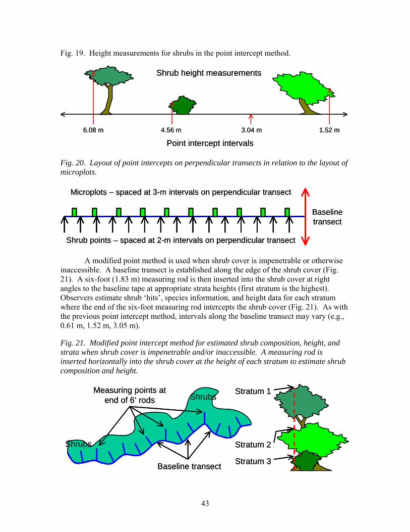
43
Fig. 19. Height measurements for shrubs in the point intercept method.
1.52 m3.04 m4.56 m6.08 m
Point intercept intervals
Shrub height measurements
1.52 m3.04 m4.56 m6.08 m
Point intercept intervals
Shrub height measurements
Fig. 20. Layout of point intercepts on perpendicular transects in relation to the layout of microplots.
Microplots – spaced at 3-m intervals on perpendicular transect
Shrub points – spaced at 2-m intervals on perpendicular transect
Baseline transect
Microplots – spaced at 3-m intervals on perpendicular transect
Shrub points – spaced at 2-m intervals on perpendicular transect
Baseline transect
A modified point method is used when shrub cover is impenetrable or otherwise inaccessible. A baseline transect is established along the edge of the shrub cover (Fig. 21). A six-foot (1.83 m) measuring rod is then inserted into the shrub cover at right angles to the baseline tape at appropriate strata heights (first stratum is the highest). Observers estimate shrub ‘hits’, species information, and height data for each stratum where the end of the six-foot measuring rod intercepts the shrub cover (Fig. 21). As with the previous point intercept method, intervals along the baseline transect may vary (e.g., 0.61 m, 1.52 m, 3.05 m).
Fig. 21. Modified point intercept method for estimated shrub composition, height, and strata when shrub cover is impenetrable and/or inaccessible. A measuring rod is inserted horizontally into the shrub cover at the height of each stratum to estimate shrub composition and height.
Measuring points at end of 6’ rods
Baseline transect
Shrubs
Shrubs
Stratum 1
Stratum 2
Stratum 3
Measuring points at end of 6’ rods
Baseline transect
Shrubs
Shrubs
Stratum 1
Stratum 2
Stratum 3

44
Shrubs can also be partitioned by type depending on preference. For example, preferred shrubs for deer do not include rabbitbrush whereas hydrophytic shrubs for yellow warblers include quaking aspen, cottonwood, water birch, willow, woods rose, red osier dogwood, and chokecherry.
Methods for Forest and Riparian Habitats
Baseline transects are about 300 meters in length, partitioned into 30-meter sampling units. Each baseline transect is oriented along a random azimuth when possible, but in riparian areas, the transects, by definition, follow the course of the riparian area. The size of the sample area strongly influences transect length. In small cover types, data from several short (100-m) transects may be ‘pooled’ in order to obtain adequate data. Transect start, end and turn points are permanently marked with a 36-centimeter (14-inch) long 0.6-centimeter (¼-inch) rebar stakes painted fluorescent orange or red.
Each transect is documented with photos from the start point. One photograph is taken along the baseline transect facing the transect direction. The camera is positioned one meter above the ground for the photo or photos (use one meter cover board or similar device for camera rest). For each photo use a 1.5-meter cover board (1.5 m X 0.1 m rectangle with alternating white and red bands at 0.1-m intervals) 10-meters in front of the camera as well as the transect photo board (relevant information for transect identification). If vegetation is too dense, photograph from a point along side or perpendicular to the transect. Record camera type, aperture, distance and azimuth to cover board, cover board dimensions, date, time of day, transect/location identification, GPS coordinates, and photographer.
Two different configurations are used to sample snag and/or tree basal area information. In one, information is collected from within 0.04 ha circular plots (radius of 11.3 m) located at 30-meter intervals along the baseline transect (Fig. 22). In the other configuration, information is collected from within areas of the same size (0.04 ha), but configured as rectangular belts (100’ X 44’ or 30.48 m X 13.41 m). The rectangular belts configured end-to-end and centered on the baseline transect with the long axis paralleling the transect (Fig. 23).
Fig. 22. Design of one type of transects in forest and riparian cover types. The circles represent 0.04 ha areas (11.3 m radius from the center point) used for estimation of tree and snag density and tree basal cover. Other characteristics such as shrub and tree composition and herbaceous cover are measured along the baseline at standardized intervals.
0 30 60 90 120 150 180 210 240 270 300
Baseline transect – 300 m
0 30 60 90 120 150 180 210 240 270 300
Baseline transect – 300 m
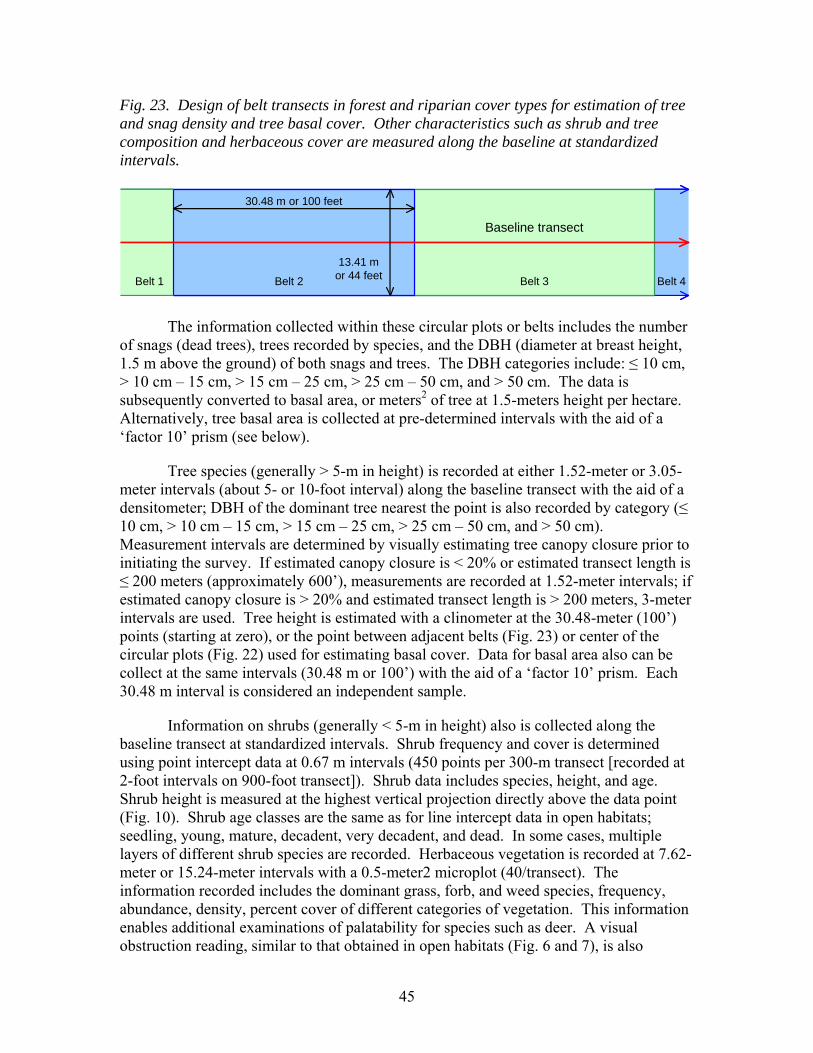
45
Fig. 23. Design of belt transects in forest and riparian cover types for estimation of tree and snag density and tree basal cover. Other characteristics such as shrub and tree composition and herbaceous cover are measured along the baseline at standardized intervals.
Baseline transect
30.48 m or 100 feet
13.41 m or 44 feetBelt 1 Belt 2 Belt 3 Belt 4
Baseline transect
30.48 m or 100 feet
13.41 m or 44 feetBelt 1 Belt 2 Belt 3 Belt 4
The information collected within these circular plots or belts includes the number of snags (dead trees), trees recorded by species, and the DBH (diameter at breast height, 1.5 m above the ground) of both snags and trees. The DBH categories include: ≤ 10 cm, > 10 cm – 15 cm, > 15 cm – 25 cm, > 25 cm – 50 cm, and > 50 cm. The data is subsequently converted to basal area, or meters2 of tree at 1.5-meters height per hectare. Alternatively, tree basal area is collected at pre-determined intervals with the aid of a ‘factor 10’ prism (see below).
Tree species (generally > 5-m in height) is recorded at either 1.52-meter or 3.05-meter intervals (about 5- or 10-foot interval) along the baseline transect with the aid of a densitometer; DBH of the dominant tree nearest the point is also recorded by category (≤ 10 cm, > 10 cm – 15 cm, > 15 cm – 25 cm, > 25 cm – 50 cm, and > 50 cm). Measurement intervals are determined by visually estimating tree canopy closure prior to initiating the survey. If estimated canopy closure is < 20% or estimated transect length is ≤ 200 meters (approximately 600’), measurements are recorded at 1.52-meter intervals; if estimated canopy closure is > 20% and estimated transect length is > 200 meters, 3-meter intervals are used. Tree height is estimated with a clinometer at the 30.48-meter (100’) points (starting at zero), or the point between adjacent belts (Fig. 23) or center of the circular plots (Fig. 22) used for estimating basal cover. Data for basal area also can be collect at the same intervals (30.48 m or 100’) with the aid of a ‘factor 10’ prism. Each 30.48 m interval is considered an independent sample.
Information on shrubs (generally < 5-m in height) also is collected along the baseline transect at standardized intervals. Shrub frequency and cover is determined using point intercept data at 0.67 m intervals (450 points per 300-m transect [recorded at 2-foot intervals on 900-foot transect]). Shrub data includes species, height, and age. Shrub height is measured at the highest vertical projection directly above the data point (Fig. 10). Shrub age classes are the same as for line intercept data in open habitats; seedling, young, mature, decadent, very decadent, and dead. In some cases, multiple layers of different shrub species are recorded. Herbaceous vegetation is recorded at 7.62-meter or 15.24-meter intervals with a 0.5-meter2 microplot (40/transect). The information recorded includes the dominant grass, forb, and weed species, frequency, abundance, density, percent cover of different categories of vegetation. This information enables additional examinations of palatability for species such as deer. A visual obstruction reading, similar to that obtained in open habitats (Fig. 6 and 7), is also
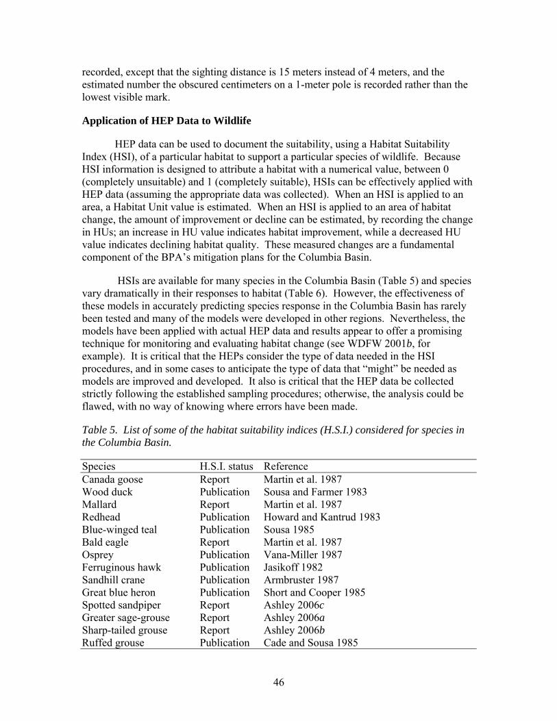
46
recorded, except that the sighting distance is 15 meters instead of 4 meters, and the estimated number the obscured centimeters on a 1-meter pole is recorded rather than the lowest visible mark.
Application of HEP Data to Wildlife
HEP data can be used to document the suitability, using a Habitat Suitability Index (HSI), of a particular habitat to support a particular species of wildlife. Because HSI information is designed to attribute a habitat with a numerical value, between 0 (completely unsuitable) and 1 (completely suitable), HSIs can be effectively applied with HEP data (assuming the appropriate data was collected). When an HSI is applied to an area, a Habitat Unit value is estimated. When an HSI is applied to an area of habitat change, the amount of improvement or decline can be estimated, by recording the change in HUs; an increase in HU value indicates habitat improvement, while a decreased HU value indicates declining habitat quality. These measured changes are a fundamental component of the BPA’s mitigation plans for the Columbia Basin.
HSIs are available for many species in the Columbia Basin (Table 5) and species vary dramatically in their responses to habitat (Table 6). However, the effectiveness of these models in accurately predicting species response in the Columbia Basin has rarely been tested and many of the models were developed in other regions. Nevertheless, the models have been applied with actual HEP data and results appear to offer a promising technique for monitoring and evaluating habitat change (see WDFW 2001b, for example). It is critical that the HEPs consider the type of data needed in the HSI procedures, and in some cases to anticipate the type of data that “might” be needed as models are improved and developed. It also is critical that the HEP data be collected strictly following the established sampling procedures; otherwise, the analysis could be flawed, with no way of knowing where errors have been made.
Table 5. List of some of the habitat suitability indices (H.S.I.) considered for species in the Columbia Basin.
Species H.S.I. status Reference Canada goose Report Martin et al. 1987 Wood duck Publication Sousa and Farmer 1983 Mallard Report Martin et al. 1987 Redhead Publication Howard and Kantrud 1983 Blue-winged teal Publication Sousa 1985 Bald eagle Report Martin et al. 1987 Osprey Publication Vana-Miller 1987 Ferruginous hawk Publication Jasikoff 1982 Sandhill crane Publication Armbruster 1987 Great blue heron Publication Short and Cooper 1985 Spotted sandpiper Report Ashley 2006c Greater sage-grouse Report Ashley 2006a Sharp-tailed grouse Report Ashley 2006b Ruffed grouse Publication Cade and Sousa 1985

47
Blue (dusky) grouse Publication Schroeder 1984 California quail Report Ashley 2006c Spotted owl Publication Layman et al. 1985 Belted kingfisher Publication Prose 1985 Hairy woodpecker Publication Sousa 1987 Downy woodpecker Publication Schroeder 1982a Lewis’ woodpecker Publication Sousa 1982 Williamson’s sapsucker Publication Sousa 1983 Pileated woodpecker Publication Schroeder 1982b Black-capped chickadee Publication Schroeder 1983a Marsh wren Publication Gutzwiller 1987 Yellow warbler Publication Schroeder 1982d Brewer’s sparrow Publication Short 1984 Western meadowlark Publication Ashley 2006 (from Schroeder and Sousa 1982) Red-winged blackbird Publication Short 1985 Yellow-headed blackbird Publication Schroeder 1982c Beaver Publication Allen 1983a Muskrat Publication Allen and Hoffman 1984 Fox squirrel Publication Allen 1982a Snowshoe hare Publication Carreker 1985 Fisher Publication Allen 1983b Mink Publication Allen 1984b Marten Publication Allen 1982b Mule deer Report Ashley and Berger 1999 White-tailed deer Report Martin et al. 1987
Table 6. Sample of focal species and the habitats and habitat features with which they are associated (adapted from Ashley and Stovall 2004a,b). A focal species and/or habitat in one subbasin was not necessarily considered in other subbasins, even if the species and/or habitat was present. In addition, focal species associated with habitats that were not substantially present on the Wildlife Areas were not considered here.
Species Habitat Type Key Feature Indicator Canopy > 70% and height > 12 m Sagebrush height > 50 cm Elk Ponderosa
Pine Herbaceous cover > 10%
Healthy forest canopy intermixed with openings for foraging
Preferred shrub cover 30-60% Preferred shrubs 1-1.5 m Mule deer Shrubsteppe At least 3 preferred shrub species
Healthy and diverse shrub layer
Bighorn sheep Grassland Steep grassy areas close to escape cover such as rocky outcrops
Grass/forb cover intermixed with steep rocky escape cover
Western gray squirrel
Ponderosa Pine
Prefers mixed stands of Ponderosa pine and oak; large pines essential
Healthy mix of pine mixed with oak
Pygmy rabbit Shrubsteppe Sagebrush cover > 20% and > 1 m in height in deep soils
Healthy shrubsteppe habitat in deep soils
Beaver Riparian Tree/shrub canopy 40-60% Healthy regenerating
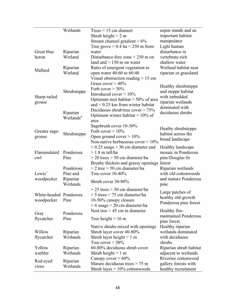
48
Trees < 15 cm diamert Shrub height > 2 m
Wetlands
Stream channel gradient < 6%
aspen stands and an important habitat manipulator
Tree grove > 0.4 ha < 250 m from water Great blue
heron Riparian Wetland Disturbance-free zone > 250 m on
land and > 150 m on water
Light human disturbance in vertebrate-rich shallow water
Mallard Riparian Wetland
Ratio of emergent vegetation to open water 40:60 to 60:40
Wetland habitat near riparian or grassland
Visual obstruction reading > 15 cm Grass cover > 40% Forb cover > 30% Introduced cover < 10% Shrubsteppe
Optimum nest habitat > 50% of area and < 0.25 km from winter habitat Deciduous shrub/tree cover > 75%
Sharp-tailed grouse
Riparian Wetlandsa Optimum winter habitat > 10% of
area
Healthy shrubsteppe and steppe habitat with imbedded riparian wetlands dominated with deciduous shrubs
Sagebrush cover 10-30% Forb cover > 10% Open ground cover > 10%
Greater sage-grouse Shrubsteppe
Non-native herbaceous cover < 10%
Heathy shrubsteppe habitat across the broad landscape
> 0.25 snags > 30 cm diameter and > 1.8 m tall/ha > 20 trees > 50 cm diameter/ha
Flammulated owl
Ponderosa Pine
Brushy thickets and grassy openings
Healthy landscape mosaic in Ponderosa pine/Douglas fir forest
> 2 tree > 50 cm diameter/ha Tree cover 10-40% Lewis’
woodpecker
Ponderosa Pine and Riparian Wetlands Shrub cover 30-80%
Riparian wetlands with old cottonwoods and mature Ponderosa pine
> 25 trees > 50 cm diameter/ha > 5 trees > 75 cm diameter/ha 10-50% canopy closure
White-headed woodpecker
Ponderosa Pine
> 4 snags > 20 cm diameter/ha
Large patches of healthy old-growth Ponderosa pine forest
Nest tree > 45 cm in diameter Gray flycatcher
Ponderosa Pine Tree height > 16 m
Healthy fire-maintained Ponderosa pine forest.
Native shrubs mixed with openings Shrub layer cover 40-80% Shrub layer height > 1 m
Willow flycatcher
Riparian Wetlands
Tree cover < 30%
Healthy riparian wetlands dominated with deciduous shrubs
60-80% deciduous shrub cover Yellow warbler
Riparian Wetlands Shrub height > 1 m
Riparian shrub habitat adjacent to wetlands
Canopy cover > 60% Mature deciduous trees > 75 m Red-eyed
vireo Riparian Wetlands Shrub layer > 10% cottonwoods
Riverine cottonwood gallery forests with healthy recruitment
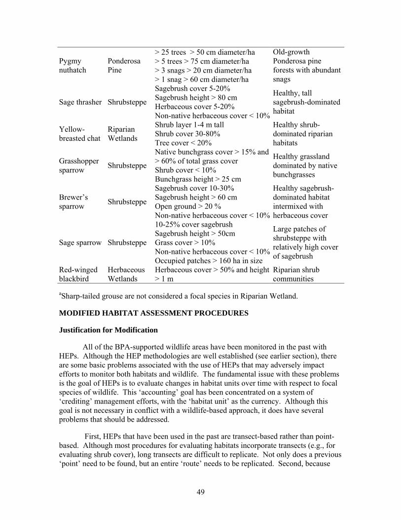
49
> 25 trees > 50 cm diameter/ha > 5 trees > 75 cm diameter/ha > 3 snags > 20 cm diameter/ha
Pygmy nuthatch
Ponderosa Pine
> 1 snag > 60 cm diameter/ha
Old-growth Ponderosa pine forests with abundant snags
Sagebrush cover 5-20% Sagebrush height > 80 cm Herbaceous cover 5-20% Sage thrasher Shrubsteppe
Non-native herbaceous cover < 10%
Healthy, tall sagebrush-dominated habitat
Shrub layer 1-4 m tall Shrub cover 30-80% Yellow-
breasted chat Riparian Wetlands Tree cover < 20%
Healthy shrub-dominated riparian habitats
Native bunchgrass cover > 15% and > 60% of total grass cover Shrub cover < 10%
Grasshopper sparrow Shrubsteppe
Bunchgrass height > 25 cm
Healthy grassland dominated by native bunchgrasses
Sagebrush cover 10-30% Sagebrush height > 60 cm Open ground > 20 %
Brewer’s sparrow Shrubsteppe
Non-native herbaceous cover < 10%
Healthy sagebrush-dominated habitat intermixed with herbaceous cover
10-25% cover sagebrush Sagebrush height > 50cm Grass cover > 10% Non-native herbaceous cover < 10%
Sage sparrow Shrubsteppe
Occupied patches > 160 ha in size
Large patches of shrubsteppe with relatively high cover of sagebrush
Red-winged blackbird
Herbaceous Wetlands
Herbaceous cover > 50% and height > 1 m
Riparian shrub communities
aSharp-tailed grouse are not considered a focal species in Riparian Wetland.
MODIFIED HABITAT ASSESSMENT PROCEDURES
Justification for Modification
All of the BPA-supported wildlife areas have been monitored in the past with HEPs. Although the HEP methodologies are well established (see earlier section), there are some basic problems associated with the use of HEPs that may adversely impact efforts to monitor both habitats and wildlife. The fundamental issue with these problems is the goal of HEPs is to evaluate changes in habitat units over time with respect to focal species of wildlife. This ‘accounting’ goal has been concentrated on a system of ‘crediting’ management efforts, with the ‘habitat unit’ as the currency. Although this goal is not necessary in conflict with a wildlife-based approach, it does have several problems that should be addressed.
First, HEPs that have been used in the past are transect-based rather than point-based. Although most procedures for evaluating habitats incorporate transects (e.g., for evaluating shrub cover), long transects are difficult to replicate. Not only does a previous ‘point’ need to be found, but an entire ‘route’ needs to be replicated. Second, because

50
transects can be long, they may cross cover types that were thought to be insignificant at the time, or perhaps non-existent at the time (perhaps altered due to management activity and/or unplanned event such as a fire). Third, transects do not offer an effective tool for linking habitat data with wildlife data. Methods for surveying wildlife are often point-based to a certain degree. Even when a wildlife survey is based on transects, transect are unlikely to be directly compatible with the HEP transects. Fourth, there is a tradeoff between the time spent sampling a unit and the number of units that can be sampled. Long transects reduce the number of units that can be sampled with the available resources. Fifth, past HEP transects have focused on characteristics of the habitat that were associated with specific habitat suitability indices (HSIs) for specific species of wildlife in specific habitats. Consequently, the data collected were not necessarily consistent between transects. The problem with this approach over the long term is that it offers limited opportunities for adaptive management. Many of the HSIs currently used have not been adequately tested. It’s possible that future models will be different than the current models and past HEPs may not be versatile enough to allow future models to be tested.
We recommend a modified habitat assessment that uses random points on wildlife areas as the foundational unit for monitoring and evaluating habitat. Although locations are selected randomly, there are additional considerations. For example, survey locations are stratified by cover type, management activities, and/or historical considerations. For example, even though points form the basis for the monitoring procedure, many of the points are linked up with HEP transects that have been monitored in the past. Although it is difficult to exactly replicate past surveys, coordination offers insight into long-term changes. The number of points to be surveyed within each ‘cover’ type ultimately reflects the size of the area, the diversity of cover types, and the goals for detecting changes in habitat.
The habitat at monitoring and evaluation points is assessed with consistent methodologies, regardless of the different wildlife species associated with the habitat. This consistency will improve the versatility of the techniques with long-term monitoring of both habitat and wildlife. This does not mean that current habitat suitability indices for wildlife are not considered. Techniques for collection of habitat data are used that insure the collection of useful data, and that the data is consistent with established models. Most HSI models use similar parameters such as percent cover of grasses, forbs, herbaceous species (grasses and forbs combined), and shrubs. Average heights are also commonly used. Many models also consider specific species. Fortunately, if the data is collected by species, these can be grouped up later without altering the field methods. Many of the models also incorporate slope and/or landscape features (e.g., distance to cropland or other alternate habitat or percent cover of a particular habitat within a pre-determined distance). In most cases these characteristics can be gathered remotely with Geographical Information Systems. However, this is not always the case. For example, the HSI for the western meadowlark uses the distance to a suitable perch (shrub, fence post, etc.) as a characteristic. Consequently, it is important to have a place on a data form for characteristics such as this. The most difficult situations are those that combine characteristics into one modeling objective. For example, the mule deer model (Ashley
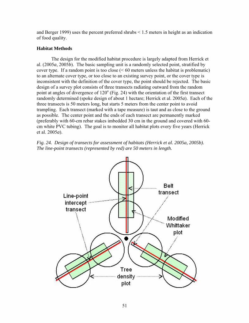
51
and Berger 1999) uses the percent preferred shrubs < 1.5 meters in height as an indication of food quality.
Habitat Methods
The design for the modified habitat procedure is largely adapted from Herrick et al. (2005a, 2005b). The basic sampling unit is a randomly selected point, stratified by cover type. If a random point is too close (< 60 meters unless the habitat is problematic) to an alternate cover type, or too close to an existing survey point, or the cover type is inconsistent with the definition of the cover type, the point should be rejected. The basic design of a survey plot consists of three transects radiating outward from the random point at angles of divergence of 120o (Fig. 24) with the orientation of the first transect randomly determined (spoke design of about 1 hectare; Herrick et al. 2005a). Each of the three transects is 50 meters long, but starts 5 meters from the center point to avoid trampling. Each transect (marked with a tape measure) is taut and as close to the ground as possible. The center point and the ends of each transect are permanently marked (preferably with 60-cm rebar stakes imbedded 30 cm in the ground and covered with 60-cm white PVC tubing). The goal is to monitor all habitat plots every five years (Herrick et al. 2005a).
Fig. 24. Design of transects for assessment of habitats (Herrick et al. 2005a, 2005b). The line-point transects (represented by red) are 50 meters in length.

52
In some situations (i.e., riparian corridors), it is impossible to place a plot in the configuration of a spoke design. In these cases, the transect is oriented perpendicular to the habitat feature, but threw the random point. In the case of a narrow riparian corridor, the transect starts 5 meters outside the riparian corridor and extends across the habitat to 5 meters beyond the other side (maximum of 50 meters). Additional transects are placed parallel to the first transect (perpendicular to the habitat feature), but separated by 25 meters. The combined transect distance for the plot is between 120 and 180 meters.
All points are monitored with photos based on standard protocols (Hall 2002). Photos of previously conducted HEP transects are also replicated when possible. In all cases the photos are used to provide a qualitative assessment of long-term changes. In order to insure their usefulness, digital photos and hard copies are labeled with appropriate reference information (e.g., date, UTM Zone, UTM, and direction). A photo point board (chalk or whiteboard) is used to in the lower part of the photo to provide a reference label. Each photo is taken at a height of 1.5 meters directly over the center stake and in the direction of each transect. In the case of riparian transects with no center point, photos are taken from the start of each transect and in the direction of the transect. In addition, photos are taken from the center of drainages, facing upstream and downstream.
The line-point intercept is the fundament technique used to assess habitat on each transect. In order to avoid trampling at the start and end of each transect, the intercept ‘points’ are at each ½ meter on the line (50 points per 50-meter transect or 150 points per plot, fewer with shorter transects). A wire pin dropped vertically from a predetermined height or a laser pointer adjacent to the tape is used to determine what is intercepted. The laser pointer also works best in an area with overhead cover (trees). Every species intercepted is recorded from top to bottom, but each species intercepted is recorded only once. In addition to plants, the surface of the ground at the intercept point is recorded: rock fragment (> 5 mm in diameter), bedrock, litter (detached dead stems and leaves in contact with the ground), woody litter (greater than 5 mm in diameter and in direct contact with soil), embedded litter (removal of litter would leave indentation in soil surface), duff (no clear boundary between litter and soil), moss, lichen crust on soil, lichen crust on rock, soil, and bare ground (occurs only when there is no top canopy). If a plant species is not known it can be recorded by genus, annual forb, perennial forb, annual grass, perennial grass, shrub, or tree. Unknown specimens are collected and referenced on the data sheet by number so that they can be identified later (Appendix C, Herrick et al. 2005b).
Following collection of the line-point intercept data, the same transects are used to record the height and species of the nearest tree (if present), shrub (if present), and herbaceous species (grass or forb) to each 5-meter interval on the tape (not counting the start and finish for each line). The heights are recorded to the nearest cm as drop height (or rounded to nearest 10-cm or meter depending on the height of the shrub or tree); do not extend the leaves to make a measurement. In addition to plant height, visual obstruction readings are taken in non-forested habitats with the aid of a Robel pole (Robel et al. 1970) at each 5-meter interval (not counting the start and finish for each line). The Robel pole is placed at the 5-meter marks on the line and the observer records
53
the 5-cm portions of the pole that are obstructed from a distance of 4 meters away from the transect.
A belt transect is used to record invasive species in non-forested habitats (Appendix C, Herrick et al. 2005b). Although the width of the belt transect can be varied depending on the density of species to be counted, we recommend using the same 1.5-meter pole that is used to standardize photos. This same pole also can be used as the Robel pole. The transect should be along the side the three 50-meter transects (Fig. 24). We recommend using the transect as an outer edge and walking alongside the transect, rather than on top of the transect. All invasive plants are counted that have at least half their base rooted under the PVC pipe.
A modified Whittaker approach is used to evaluate species richness (Appendix C, Herrick et al. 2005b). A 10 X 30-meter plot is centered on each of the three transects starting at the 5-meter mark (Fig. 24). The long side of the rectangle is parallel to the line-point intercept transect (Herrick et al. 2005a). All species observed in each area are recorded.
In forested habitats, circular plots with a radius of 11.3 meters (0.04 ha in area) are used to sample snag and/or tree basal area (Appendix C, Herrick et al. 2005b). With transects of 50 meters, one circle is centered at the 10-meter mark and the other is centered at the 35-meter mark (Fig. 24). With shorter transects, the circle is placed at the midpoint of the transect. The information collected within these circular plots includes the number of snags (dead trees), trees recorded by species, and the DBH (diameter at breast height, 1.5 m above the ground) of both snags and trees. The DBH categories include: ≤ 10 cm, > 10 cm – 15 cm, > 15 cm – 25 cm, > 25 cm – 50 cm, and > 50 cm. The data is subsequently converted to basal area, or meters2 of tree at 1.5-meters height per hectare. Alternatively, tree basal area can be collected at pre-determined intervals with the aid of a ‘factor 10’ prism.
In general, the habitat methods are designed to be consistent, regardless of the focal species present in a particularly area. The methods are also designed to collect the vast majority of the data needed to evaluate habitat suitability indices for many of the species (Table 5 and 6). The primary exceptions are when landscape data is needed, such as the distance to a specific habitat type or the area of a habitat patch. However, it is doubtful that this type of data could be collected as efficiently in the field as it can be with the aid of Geographical Information Systems.
WILDLIFE MONITORING AND EVALUATION
Monitoring consists of trend studies (measuring change over time), baseline studies, long-term ecological studies, and basic inventories. Monitoring and evaluation are directed towards wildlife or the habitats upon which they depend. Protocols and techniques are subject to modification as new information and techniques become available (Ashley and Stovall 2004a,b). The following four basic types of monitoring and evaluation surveys have been, or are being conducted: 1) HEP surveys (five-year intervals); 2) modified habitat assessments (five-year intervals); 3) Site specific

54
enhancement and maintenance activity surveys (one- to five-year intervals); and 4) Wildlife species response/trend surveys (one- to three-year intervals).
Several specific techniques are being used to monitor and evaluate wildlife populations on wildlife areas. Several high profile, threatened and endangered, unusually distributed, and/or rare species may survey techniques that are species specific. In contrast, other relatively common and somewhat evenly distributed species may be monitored with surveys that permit several species to be surveyed simultaneously.
The number of techniques that can provide insight to animal abundance and distribution is virtually limitless. The descriptions below focus on techniques that are relatively standard, and hence, somewhat universal and repeatable. In addition, the following discussion deals mostly with techniques that are currently being used to address focal species. However, there are many regular surveys that are being conducted on non-focal species. The results of these surveys will offer critical insight into the relationship between focal species and the ecosystems they represent. Consequently, we also provide a discussion of additional survey techniques and the species that may be addressed.
Pygmy Rabbit
Data on populations and trends of pygmy rabbits have been based on burrow surveys (WDFW 1995). Burrow surveys consist of: 1) Counts conducted between late autumn and early spring; 2) 100% surveys within randomly-selected circular sub-samples of larger areas; 3) Description of the openness of the burrow passages; and 4) Presence and appearance of fecal pellets. Application of this technique in the SFWA has been closely associated with other estimates of population abundance (WDFW 1995, Hays 2003). A more statistically defensible procedure, such as a capture-recapture technique, has not been developed for pygmy rabbits. Because of the extirpation of pygmy rabbits in the state, burrow surveys are not currently being conducted. These will be resumed once a population has been re-established.
Beaver
Surveys for beavers focus on the direct observations of beavers and the presence of fresh sign, such as beaver-cut trees and/or food caches (Smith 1998). Because beavers accumulate freshly cut branches in floating caches adjacent to their lodges, the presence of these caches is used to establish presence. Caches are detected with ground surveys, or relatively efficiently by aerial surveys. Smith (1998) was able to survey more that 300 km of potential beaver habitat along rivers and streams in Yellowstone National Park with about 19 hours of fixed-wing aircraft flight time. The best time to conduct these surveys is in autumn, after most leaves have fallen from deciduous trees and before the water has frozen; this survey period usually equates to the first half of November in eastern Washington). Once each beaver colony is detected and mapped, the population is estimated by assuming an average number of 6 beavers per colony (Novak 1987).
55
Western Gray Squirrel
Surveys for western gray squirrels are focused in areas where their occurrence is likely, based on habitat suitability, and/or possible observations of animals and signs. The best way to monitor squirrels is with the identification and description of nests. The nest description should include: 1) Observation of squirrels; 2) Type of nest (shelter or platform); 3) Condition (intact or deteriorating); 4) Color (indication of condition); 5) Height in tree; and 6) DBH of nest tree (Vander Haegen et al. 2004a, 2005a). Other considerations for conducting population surveys, such as capture-recapture analyses, have not been tested on a broad scale for western gray squirrels (Vander Haegen et al. 2004a).
Big Game
Aerial surveys are an efficient and relatively inexpensive way to monitor elk. Fowler (2001) estimated that a 30-hour aerial survey by helicopter for elk would require approximately 300 hours of ground survey. Consequently, in Washington, aerial surveys are used to monitor population size and sex composition of the Blue Mountain and Yakima elk herds. Each of these surveys consists of about 10 hours of flying time in September and about 30 hours of flying time in winter (usually February or March). Approximately 70% of the survey units are flown, and a sightability factor is used to convert the number of observed elk into a population estimate (Samuel et al. 1987, WDFW 2002b). A model using information on sex, age, and harvest is used to estimate population size (Bender and Spencer 1999).
Aerial surveys are used to monitor mule deer and white-tailed deer populations in eastern Washington (supplemented with ground surveys). For both species, surveys (often ground surveys) are typically conducted during the late summer or early autumn, prior to the hunting season (WDFW 2002a, 2003). These surveys provide data on the ratio of bucks:does and legal bucks:does (legal bucks are those that can be legally harvested). Additional surveys (usually by helicopter) are conducted after the harvest in early winter (before deer shed their antlers) to estimate population size and buck survival. In the case of white-tailed deer, additional surveys may be conducted in spring to evaluate winter survival. The same tools used in elk population analysis, such as sightability considerations (Samuel et al. 1987) and population modeling (Bender and Spencer 1999), also apply to deer monitoring and evaluation.
Aerial or ground surveys are used to monitor and evaluate bighorn sheep populations (WDFW 2002a, 2003). Surveys are conducted during lambing or rutting periods and data are used to estimate lamb recruitment, sex ratio, adult survival, population size, and percentage of mature rams in the population. WDFW has an objective to monitor bighorn sheep herds at a level where a 20% change in population size can be detected within 3 years. Similar to deer and elk, sightability is considered in bighorn sheep surveys (Bodie et al. 1995).
Occasionally, aerial surveys are used for other species in the Columbia River Basin, but these surveys tend to be more opportunistic and less standardized. For

56
example, aerial surveys are often used to check raptor nests in inaccessible locations. They can also be used to find sharp-tailed grouse and greater sage-grouse display sites (leks), great blue heron nesting colonies, and beaver ponds. Despite the potential for using aerial surveys, this report will focus on techniques that are more standardized, more applicable, and in most cases less expensive.
Prairie Grouse
Male sharp-tailed grouse and greater sage-grouse (collectively referred to as prairie grouse) congregate on traditionally-occupied lek sites during the spring to display to, and breed with, females. The CCT, DOD, and WDFW annually survey most known leks, with at least 3 visits for each sage-grouse lek and as few as 1 visit to each sharp-tailed grouse lek (Schroeder et al. 2000a, b). In some areas of Washington, these surveys have been conducted since the 1950’s. In the case of greater sage-grouse, where males are readily distinguishable from females, each sex is identified and counted. In the case of sharp-tailed grouse, where males and females are difficult to distinguish from a distance, the total number of birds is recorded. The high counts, within a year, for each lek (male sage-grouse and all sharp-tailed grouse), are tallied, to estimate the total number of birds of each species. The population of sharp-tailed grouse is estimated by doubling the maximum counts within a year (assuming about half the birds are observed). The population of greater sage-grouse is estimated by multiplying the maximum counts by 2.6 (assuming that most males are counted and the sex ratio of females to males is 1.6:1.0). Although this procedure has been questioned, with regard to population estimation (Walsh et al. 2004), the technique does provide reliable information on long-term trends (Connelly et al. 2004).
Great Blue Heron
Because of their patchy distribution, great blue herons can be difficult to survey. Surveys often target key habitats associated with shallow water (Quinn and Milner 1999). In addition, because they tend to nest in colonies, one of the most useful techniques for monitoring herons is to find and monitor traditional nesting colonies. Special care should be taken to avoid disturbing these sites, as great blue herons are easily disturbed. Some of the data that should be recorded at nest sites includes: 1) Location; 2) Tree species, DBH, and height; 3) Date and time; 4) Observer; 5) Occupancy; and 6) Number of eggs, young, and fledglings (not likely obtained without disturbing the birds).
Mallard
Because mallards are widespread, abundant, and often isolated from humans, surveys from fixed-wing aircraft are typically used to monitor their populations. In Washington, aerial surveys are conducted by USFWS, YIN, and WDFW biologists in mid-winter and sometimes during the summer breeding season. In cases where rivers are surveyed, two trained biologists are on each flight, so that both sides of the aircraft can be monitored. When this is done in Washington, all duck species are recorded; hence, the same survey can be used to monitor many species in addition to mallards. Care is taken to control for missed sections of river and/or lakes, so that long-term trends are not biased
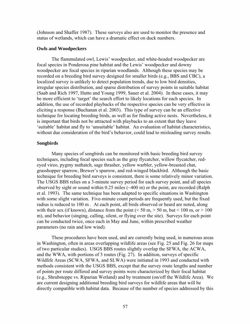
57
(Johnson and Shaffer 1987). These surveys also are used to monitor the presence and status of wetlands, which can have a dramatic effect on duck numbers.
Owls and Woodpeckers
The flammulated owl, Lewis’ woodpecker, and white-headed woodpecker are focal species in Ponderosa pine habitat and the Lewis’ woodpecker and downy woodpecker are focal species in riparian woodlands. Although these species may be recorded on a breeding bird survey designed for smaller birds (e.g., BBS and CBC), a localized survey is unlikely to detect population trends, due to low bird densities, irregular species distribution, and sparse distribution of survey points in suitable habitat (Saab and Rich 1997, Hutto and Young 1999, Sauer et al. 2004). In these cases, it may be more efficient to ‘target’ the search effort to likely locations for each species. In addition, the use of recorded playbacks of the respective species can be very effective in eliciting a response (Buchanan et al. 2003). This type of survey can be an effective technique for locating breeding birds, as well as for finding active nests. Nevertheless, it is important that birds not be attracted with playbacks to an extent that they leave ‘suitable’ habitat and fly to ‘unsuitable’ habitat. An evaluation of habitat characteristics, without due consideration of the bird’s behavior, could lead to misleading survey results.
Songbirds
Many species of songbirds can be monitored with basic breeding bird survey techniques, including focal species such as the gray flycatcher, willow flycatcher, red-eyed vireo, pygmy nuthatch, sage thrasher, yellow warbler, yellow-breasted chat, grasshopper sparrow, Brewer’s sparrow, and red-winged blackbird. Although the basic technique for breeding bird surveys is consistent, there is some relatively minor variation. The USGS BBS relies on a 3-minute survey period for each survey point, and all species observed by sight or sound within 0.25 miles (~400 m) or the point, are recorded (Ralph et al. 1993). The same technique has been adapted to specific situations in Washington with some slight variation. Five-minute count periods are frequently used, but the fixed radius is reduced to 100 m . At each point, all birds observed or heard are noted, along with their sex (if known), distance from the point (< 50 m, > 50 m, but < 100 m, or > 100 m), and behavior (singing, calling, silent, or flying over the site). Surveys for each point can be conducted twice, once each in May and June, within prescribed weather parameters (no rain and low wind).
These procedures have been used, and are currently being used, in numerous areas in Washington, often in areas overlapping wildlife areas (see Fig. 25 and Fig. 26 for maps of two particular studies). USGS BBS routes slightly overlap the SFWA, the ACWA, and the WWA, with portions of 3 routes (Fig. 27). In addition, surveys of specific Wildlife Areas (SCWA, SFWA, and SLWA) were initiated in 1993 and conducted with methods consistent with the USGS BBS, except that the survey route lengths and number of points per route differed and survey points were characterized by their focal habitat (e.g., Shrubsteppe vs. Riparian Wetland) and by treatment (on/off the Wildlife Area). We are current designing additional breeding bird surveys for wildlife areas that will be directly compatible with habitat data. Because of the number of species addressed by this
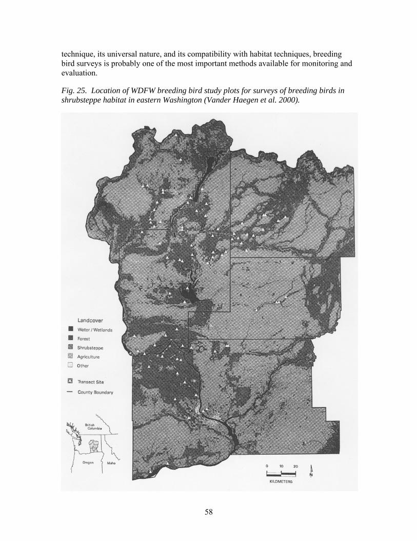
58
technique, its universal nature, and its compatibility with habitat techniques, breeding bird surveys is probably one of the most important methods available for monitoring and evaluation.
Fig. 25. Location of WDFW breeding bird study plots for surveys of breeding birds in shrubsteppe habitat in eastern Washington (Vander Haegen et al. 2000).
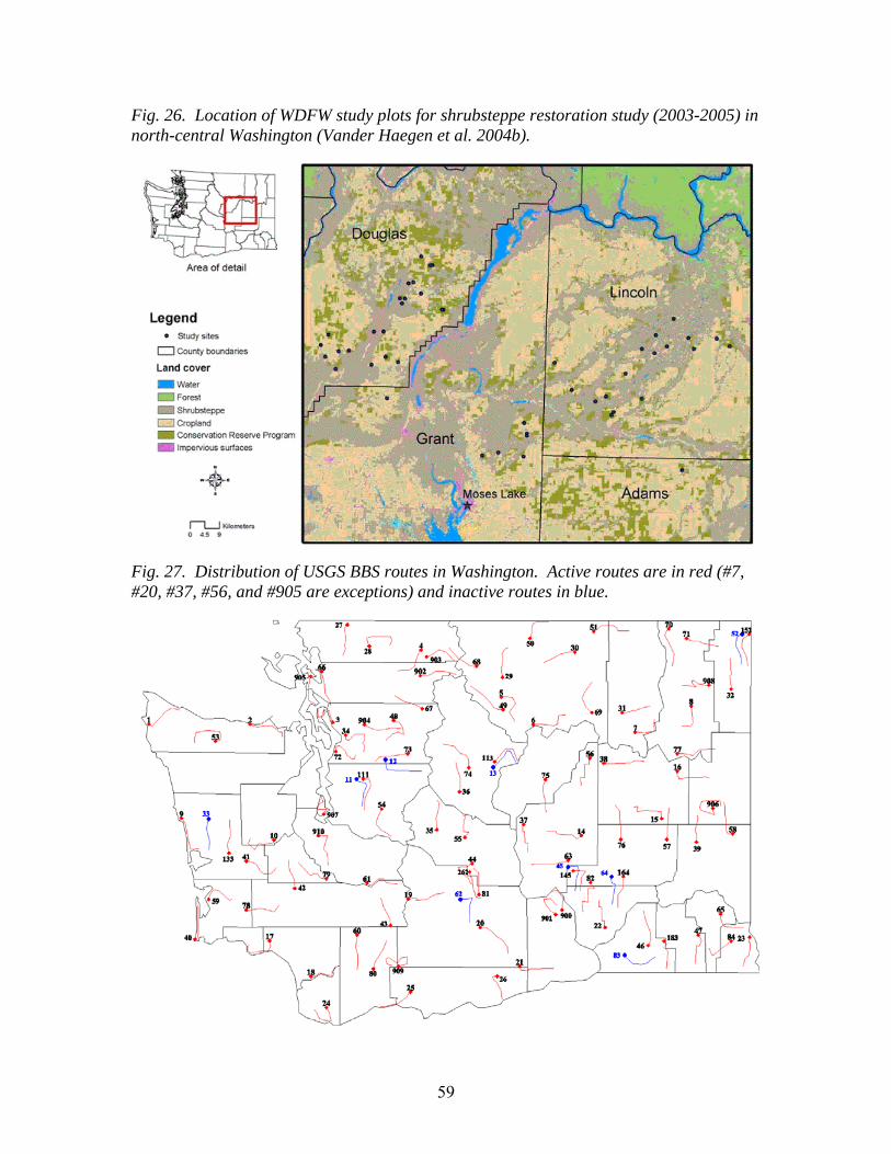
59
Fig. 26. Location of WDFW study plots for shrubsteppe restoration study (2003-2005) in north-central Washington (Vander Haegen et al. 2004b).
Fig. 27. Distribution of USGS BBS routes in Washington. Active routes are in red (#7, #20, #37, #56, and #905 are exceptions) and inactive routes in blue.
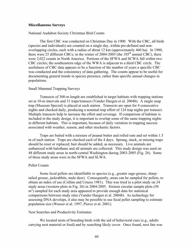
60
Miscellaneous Surveys
National Audubon Society Christmas Bird Counts
The first CBC was conducted on Christmas Day in 1900. With the CBC, all birds (species and individuals) are counted on a single day, within pre-defined and non-overlapping circles, each with a radius of about 12 km (approximately 460 ha). In 1900, there were 25 different CBCs; in the winter of 2004-2005 (the 105th annual CBC), there were 2,022 counts in North America. Portions of the SFWA and SCWA fall within two CBC circles; the southeastern edge of the WWA is adjacent to a third CBC circle. The usefulness of CBC data appears to be a function of the number of years a specific CBC was conducted and the consistency of data gathering. The counts appear to be useful for documenting general trends in species presence, rather than specific annual changes in populations.
Small Mammal Trapping Surveys
Transects of 300-m length are established in target habitats with trapping stations set at 10-m intervals and 31 traps/transect (Vander Haegen et al. 2004b). A single snap trap (Museum Special) is placed at each station. Transects are open for 4 consecutive nights and checked daily, producing a nominal trap effort of 124 trap nights per transect. Multiple transects help to increase the effort and coverage. If comparison of habitats is included in the study design, it is important to overlap some of the same trapping nights in different habitats. This is important, because of daily variation in trapping success associated with weather, season, and other stochastic factors.
Traps are baited with a mixture of peanut butter and rolled oats and set within 1.5 m of each station. Traps are checked each of the 4 days. Sprung, stuck, or missing traps should be reset or replaced; bait should be added, as necessary. Live animals are euthanized with halothane and all animals are collected. This study design was used on 48 different study areas in north-central Washington during 2003-2005 (Fig. 26). Some of these study areas were in the SFWA and SLWA.
Pellet Counts
Some fecal pellets are identifiable to species (e.g., greater sage-grouse, sharp-tailed grouse, jackrabbits, mule deer). Consequently, areas can be sampled for pellets, to obtain an index of use (Collins and Urness 1981). This was tried in a pilot study on 24 study areas (western plots in Fig. 26) in 2004-2005. Sixteen circular sample plots (50 m2) sampled for each study area appeared to provide enough data for statistical comparisons between study sites (Vander Haegen et al. 2004b). As technology for assessing DNA develops, it also may be possible to use fecal pellet sampling to estimate population size (Wasser et al. 1997, Pierce et al. 2001).
Nest Searches and Productivity Estimates
We located nests of breeding birds with the aid of behavioral cues (e.g., adults carrying nest material or food) and by searching likely cover. Once found, nest fate was
61
monitored and assessed with a modified Vickery technique (Vickery et al. 1992). This study design was used on 36 of 48 study areas in north-central Washington during 2003-2005 (Fig. 26). Some of these study areas were in the SFWA and SLWA (Vander Haegen et al. 2004b).
Reptile and Amphibian Surveys
We evaluated reptile and amphibian abundance with area- and time-constrained visual searches. These constraints are essential to reduce potential biases among observers, habitats, times, and dates. Pooling incidental observations and formal survey data results in a more thorough species list for each site, than by using formal survey information alone. Funnel traps can also be used. These study designs were used on 48 study areas in north-central Washington, during 2003-2005 (Fig. 26), some of which were in the SFWA and SLWA.
Hunter Harvest Surveys
Questionnaires (WDFW 2003, 2004a), check stations, wing barrels, bag checks, and mandatory hunter reports are used to monitor and evaluate hunter harvest. Harvest data are then used to evaluate the population in question with specific data, such as the sex ratio of the harvested species, hunter success rates, regional harvest comparisons, and age structure of the harvested population. Although all of the BPA-funded Wildlife Areas are encompassed by at least one hunter harvest survey, depending on the species of interest, some of the statistics are summarized by county, some by Game Management Unit (GMU), but none specifically by Wildlife Area.
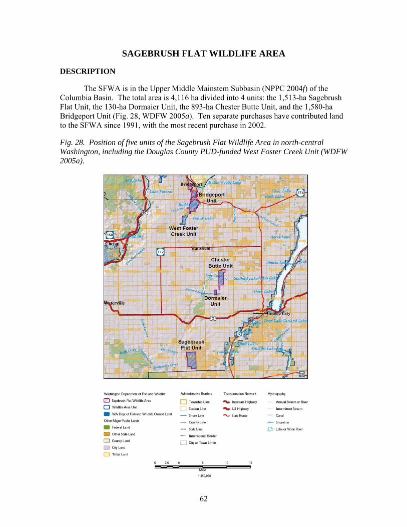
62
SAGEBRUSH FLAT WILDLIFE AREA
DESCRIPTION
The SFWA is in the Upper Middle Mainstem Subbasin (NPPC 2004f) of the Columbia Basin. The total area is 4,116 ha divided into 4 units: the 1,513-ha Sagebrush Flat Unit, the 130-ha Dormaier Unit, the 893-ha Chester Butte Unit, and the 1,580-ha Bridgeport Unit (Fig. 28, WDFW 2005a). Ten separate purchases have contributed land to the SFWA since 1991, with the most recent purchase in 2002.
Fig. 28. Position of five units of the Sagebrush Flat Wildlife Area in north-central Washington, including the Douglas County PUD-funded West Foster Creek Unit (WDFW 2005a).
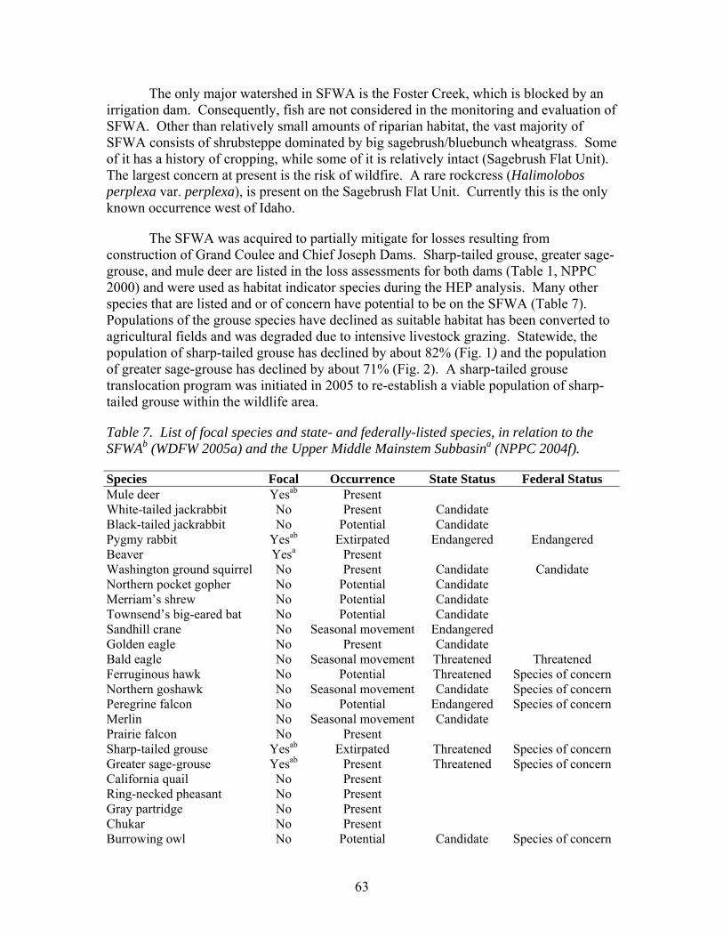
63
The only major watershed in SFWA is the Foster Creek, which is blocked by an irrigation dam. Consequently, fish are not considered in the monitoring and evaluation of SFWA. Other than relatively small amounts of riparian habitat, the vast majority of SFWA consists of shrubsteppe dominated by big sagebrush/bluebunch wheatgrass. Some of it has a history of cropping, while some of it is relatively intact (Sagebrush Flat Unit). The largest concern at present is the risk of wildfire. A rare rockcress (Halimolobos perplexa var. perplexa), is present on the Sagebrush Flat Unit. Currently this is the only known occurrence west of Idaho.
The SFWA was acquired to partially mitigate for losses resulting from construction of Grand Coulee and Chief Joseph Dams. Sharp-tailed grouse, greater sage-grouse, and mule deer are listed in the loss assessments for both dams (Table 1, NPPC 2000) and were used as habitat indicator species during the HEP analysis. Many other species that are listed and or of concern have potential to be on the SFWA (Table 7). Populations of the grouse species have declined as suitable habitat has been converted to agricultural fields and was degraded due to intensive livestock grazing. Statewide, the population of sharp-tailed grouse has declined by about 82% (Fig. 1) and the population of greater sage-grouse has declined by about 71% (Fig. 2). A sharp-tailed grouse translocation program was initiated in 2005 to re-establish a viable population of sharp-tailed grouse within the wildlife area.
Table 7. List of focal species and state- and federally-listed species, in relation to the SFWAb (WDFW 2005a) and the Upper Middle Mainstem Subbasina (NPPC 2004f).
Species Focal Occurrence State Status Federal Status Mule deer Yesab Present White-tailed jackrabbit No Present Candidate Black-tailed jackrabbit No Potential Candidate Pygmy rabbit Yesab Extirpated Endangered Endangered Beaver Yesa Present Washington ground squirrel No Present Candidate Candidate Northern pocket gopher No Potential Candidate Merriam’s shrew No Potential Candidate Townsend’s big-eared bat No Potential Candidate Sandhill crane No Seasonal movement Endangered Golden eagle No Present Candidate Bald eagle No Seasonal movement Threatened Threatened Ferruginous hawk No Potential Threatened Species of concern Northern goshawk No Seasonal movement Candidate Species of concern Peregrine falcon No Potential Endangered Species of concern Merlin No Seasonal movement Candidate Prairie falcon No Present Sharp-tailed grouse Yesab Extirpated Threatened Species of concern Greater sage-grouse Yesab Present Threatened Species of concern California quail No Present Ring-necked pheasant No Present Gray partridge No Present Chukar No Present Burrowing owl No Potential Candidate Species of concern
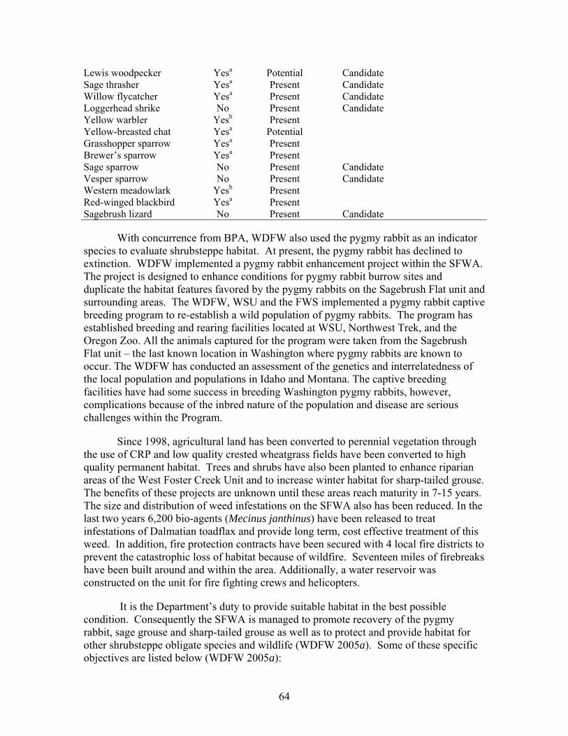
64
Lewis woodpecker Yesa Potential Candidate Sage thrasher Yesa Present Candidate Willow flycatcher Yesa Present Candidate Loggerhead shrike No Present Candidate Yellow warbler Yesb Present Yellow-breasted chat Yesa Potential Grasshopper sparrow Yesa Present Brewer’s sparrow Yesa Present Sage sparrow No Present Candidate Vesper sparrow No Present Candidate Western meadowlark Yesb Present Red-winged blackbird Yesa Present Sagebrush lizard No Present Candidate
With concurrence from BPA, WDFW also used the pygmy rabbit as an indicator species to evaluate shrubsteppe habitat. At present, the pygmy rabbit has declined to extinction. WDFW implemented a pygmy rabbit enhancement project within the SFWA. The project is designed to enhance conditions for pygmy rabbit burrow sites and duplicate the habitat features favored by the pygmy rabbits on the Sagebrush Flat unit and surrounding areas. The WDFW, WSU and the FWS implemented a pygmy rabbit captive breeding program to re-establish a wild population of pygmy rabbits. The program has established breeding and rearing facilities located at WSU, Northwest Trek, and the Oregon Zoo. All the animals captured for the program were taken from the Sagebrush Flat unit – the last known location in Washington where pygmy rabbits are known to occur. The WDFW has conducted an assessment of the genetics and interrelatedness of the local population and populations in Idaho and Montana. The captive breeding facilities have had some success in breeding Washington pygmy rabbits, however, complications because of the inbred nature of the population and disease are serious challenges within the Program.
Since 1998, agricultural land has been converted to perennial vegetation through the use of CRP and low quality crested wheatgrass fields have been converted to high quality permanent habitat. Trees and shrubs have also been planted to enhance riparian areas of the West Foster Creek Unit and to increase winter habitat for sharp-tailed grouse. The benefits of these projects are unknown until these areas reach maturity in 7-15 years. The size and distribution of weed infestations on the SFWA also has been reduced. In the last two years 6,200 bio-agents (Mecinus janthinus) have been released to treat infestations of Dalmatian toadflax and provide long term, cost effective treatment of this weed. In addition, fire protection contracts have been secured with 4 local fire districts to prevent the catastrophic loss of habitat because of wildfire. Seventeen miles of firebreaks have been built around and within the area. Additionally, a water reservoir was constructed on the unit for fire fighting crews and helicopters.
It is the Department’s duty to provide suitable habitat in the best possible condition. Consequently the SFWA is managed to promote recovery of the pygmy rabbit, sage grouse and sharp-tailed grouse as well as to protect and provide habitat for other shrubsteppe obligate species and wildlife (WDFW 2005a). Some of these specific objectives are listed below (WDFW 2005a):
65
1. Protect and restore shrubsteppe habitat. The strategies listed for these objectives are: 1) Perform shrubsteppe condition surveys to assess habitat quality issues; 2) Restore old agriculture fields and other disturbed sites to native shrubsteppe habitat; 3) Irrigate grass seeding in old orchard site as needed; 4) Control noxious weeds on the area using integrated pest management principles; 5) Maintain boundary fences to prevent trespass cattle grazing; 6) Maintain fire protection contracts with local fire districts and develop fire plans for each Unit; 7) Coordinate with other agencies and internal WDFW divisions to perform a survey for rare plants; and 8) Protect and preserve cryptogrammic soils.
2. Develop and maintain quality habitat that will provide life requisites for a diversity of species. The strategies listed for these objectives are: 1) Determine species use by performing surveys for breeding birds, amphibians, and other wildlife where practical; 2) Assess restoration efforts and use adaptive management to create and enhance shrubsteppe habitat suitable for a diversity of species; and 3) Protect shrubsteppe.
3. Protect and restore riparian habitat. The strategies listed for these objectives are: 1) Plant suitable shrubs and trees within the West Foster Creek corridor; 2) Protect newly planted shrubs and trees with deer fencing where practical; 3) Build irrigation system to water established water birch trees; and 4) Assess insect infestation of established water birch trees and release suitable bio-control agents. Coordinate with Washington State University Extension office.
4. Manage for upland birds. The SFWA was purchased to protect and enhance shrubsteppe habitat for shrubsteppe obligates. This habitat also provides habitat for upland birds and big game. Upland birds provide recreational opportunities. The strategies listed are the same as those listed above for the protection and restoration of shrubsteppe.
5. Maintain big game populations. The SFWA was purchased to protect and enhance shrubsteppe habitat for shrubsteppe obligates. This habitat also provides habitat for big game and upland birds. Big game provides recreational opportunities. In addition to the strategies listed above for the protection and restoration of shrubsteppe, the recommended strategies include using locally-collected bitterbrush seeds in seed mixes used in the restoration of critical agricultural fields.
UPPER MIDDLE MAINSTEM SUBBASIN
Because SFWA is entirely within the UMMS, the relationship between the appropriate management plan (NPPC 2004f) and the SFWA is considered here. For example, the UMMS Plan recommends the use of numerous ‘focal’ species whose life history requirements for persistence define the habitat attributes that must be present if a landscape is to meet the requirements for all species that occur there (Lambeck (1997).
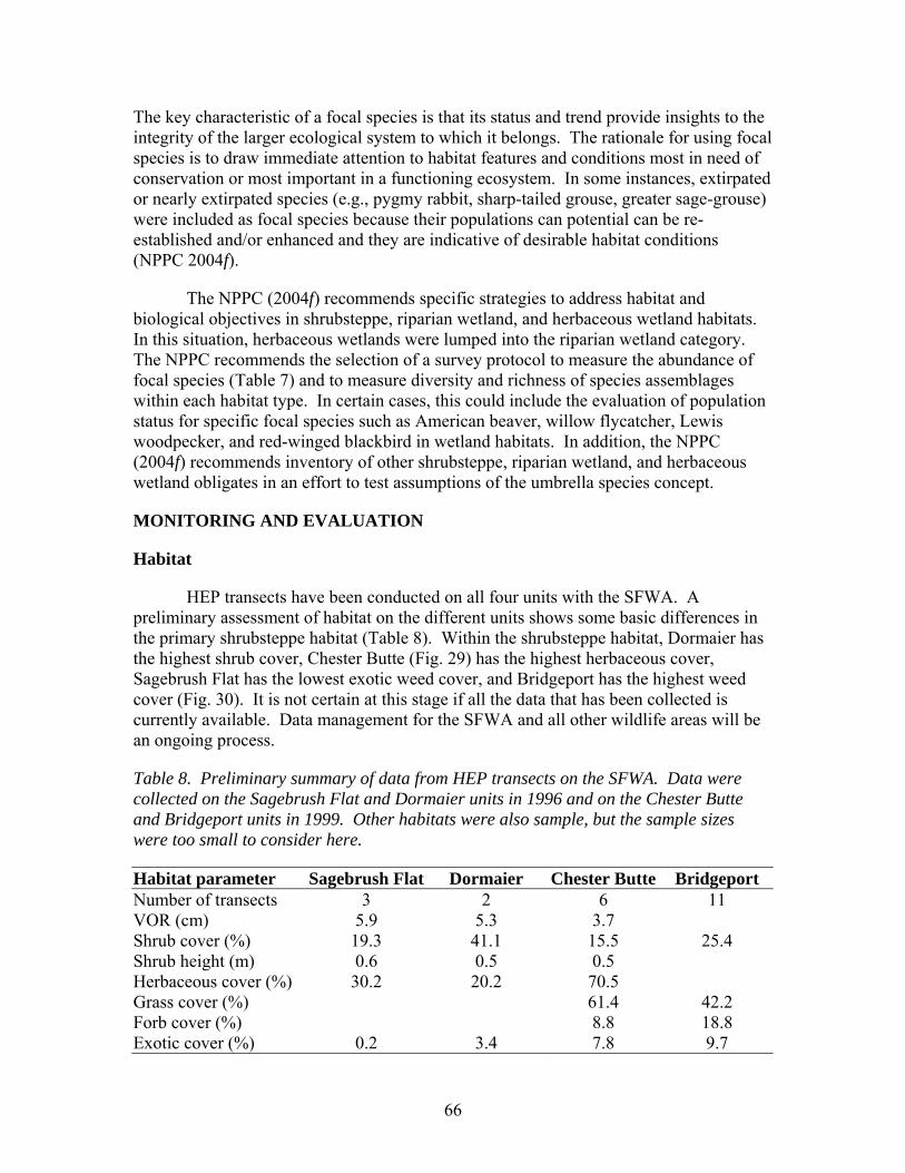
66
The key characteristic of a focal species is that its status and trend provide insights to the integrity of the larger ecological system to which it belongs. The rationale for using focal species is to draw immediate attention to habitat features and conditions most in need of conservation or most important in a functioning ecosystem. In some instances, extirpated or nearly extirpated species (e.g., pygmy rabbit, sharp-tailed grouse, greater sage-grouse) were included as focal species because their populations can potential can be re-established and/or enhanced and they are indicative of desirable habitat conditions (NPPC 2004f).
The NPPC (2004f) recommends specific strategies to address habitat and biological objectives in shrubsteppe, riparian wetland, and herbaceous wetland habitats. In this situation, herbaceous wetlands were lumped into the riparian wetland category. The NPPC recommends the selection of a survey protocol to measure the abundance of focal species (Table 7) and to measure diversity and richness of species assemblages within each habitat type. In certain cases, this could include the evaluation of population status for specific focal species such as American beaver, willow flycatcher, Lewis woodpecker, and red-winged blackbird in wetland habitats. In addition, the NPPC (2004f) recommends inventory of other shrubsteppe, riparian wetland, and herbaceous wetland obligates in an effort to test assumptions of the umbrella species concept.
MONITORING AND EVALUATION
Habitat
HEP transects have been conducted on all four units with the SFWA. A preliminary assessment of habitat on the different units shows some basic differences in the primary shrubsteppe habitat (Table 8). Within the shrubsteppe habitat, Dormaier has the highest shrub cover, Chester Butte (Fig. 29) has the highest herbaceous cover, Sagebrush Flat has the lowest exotic weed cover, and Bridgeport has the highest weed cover (Fig. 30). It is not certain at this stage if all the data that has been collected is currently available. Data management for the SFWA and all other wildlife areas will be an ongoing process.
Table 8. Preliminary summary of data from HEP transects on the SFWA. Data were collected on the Sagebrush Flat and Dormaier units in 1996 and on the Chester Butte and Bridgeport units in 1999. Other habitats were also sample, but the sample sizes were too small to consider here.
Habitat parameter Sagebrush Flat Dormaier Chester Butte Bridgeport Number of transects 3 2 6 11 VOR (cm) 5.9 5.3 3.7 Shrub cover (%) 19.3 41.1 15.5 25.4 Shrub height (m) 0.6 0.5 0.5 Herbaceous cover (%) 30.2 20.2 70.5 Grass cover (%) 61.4 42.2 Forb cover (%) 8.8 18.8 Exotic cover (%) 0.2 3.4 7.8 9.7
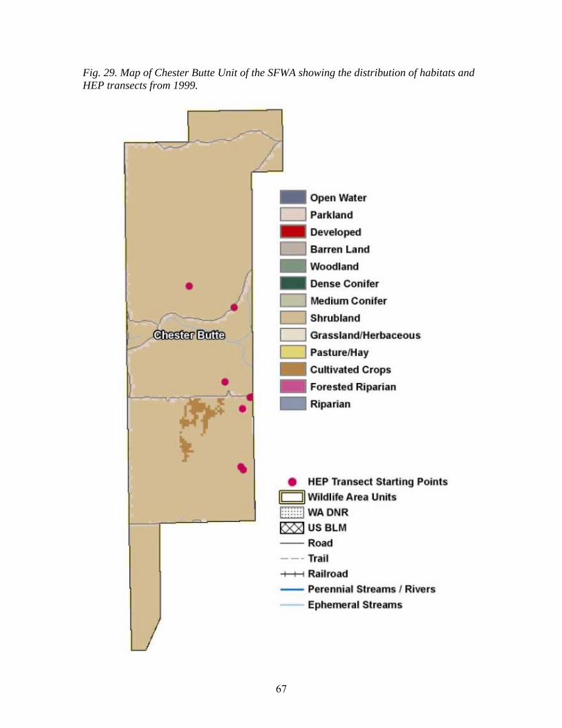
67
Fig. 29. Map of Chester Butte Unit of the SFWA showing the distribution of habitats and HEP transects from 1999.

68
Fig. 30. Map of Bridgeport Unit of the SFWA showing the distribution of habitats and HEP transects from 1999.
Mule Deer
Surveys for mule deer are regularly conducted in the region, not specifically associated with the SFWA, but to monitor populations and harvest. Both aerial and ground surveys are used to monitor populations and sex ratio (WDFW 2002a, 2003). Surveys are conducted before and after the harvest, and sightability is considered in the population estimates. Check stations and questionnaires are also used to estimate the harvest. The two GMUs containing the SFWA had an estimated harvest of 200 bucks
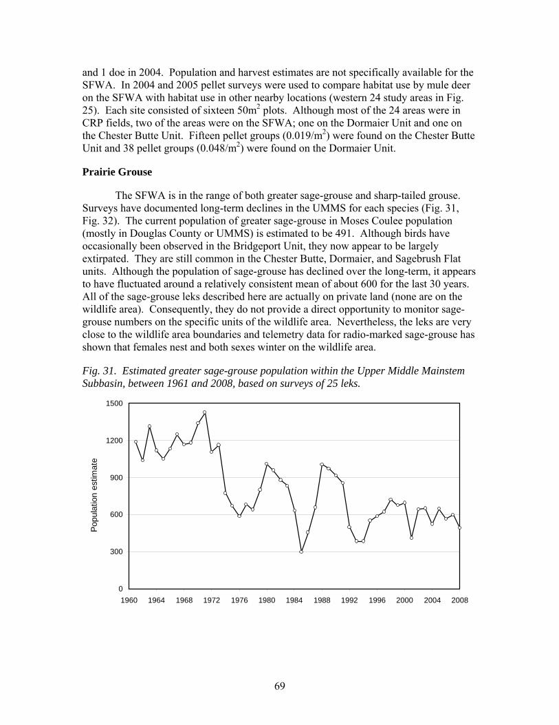
69
and 1 doe in 2004. Population and harvest estimates are not specifically available for the SFWA. In 2004 and 2005 pellet surveys were used to compare habitat use by mule deer on the SFWA with habitat use in other nearby locations (western 24 study areas in Fig. 25). Each site consisted of sixteen 50m2 plots. Although most of the 24 areas were in CRP fields, two of the areas were on the SFWA; one on the Dormaier Unit and one on the Chester Butte Unit. Fifteen pellet groups (0.019/m2) were found on the Chester Butte Unit and 38 pellet groups (0.048/m2) were found on the Dormaier Unit.
Prairie Grouse
The SFWA is in the range of both greater sage-grouse and sharp-tailed grouse. Surveys have documented long-term declines in the UMMS for each species (Fig. 31, Fig. 32). The current population of greater sage-grouse in Moses Coulee population (mostly in Douglas County or UMMS) is estimated to be 491. Although birds have occasionally been observed in the Bridgeport Unit, they now appear to be largely extirpated. They are still common in the Chester Butte, Dormaier, and Sagebrush Flat units. Although the population of sage-grouse has declined over the long-term, it appears to have fluctuated around a relatively consistent mean of about 600 for the last 30 years. All of the sage-grouse leks described here are actually on private land (none are on the wildlife area). Consequently, they do not provide a direct opportunity to monitor sage-grouse numbers on the specific units of the wildlife area. Nevertheless, the leks are very close to the wildlife area boundaries and telemetry data for radio-marked sage-grouse has shown that females nest and both sexes winter on the wildlife area.
Fig. 31. Estimated greater sage-grouse population within the Upper Middle Mainstem Subbasin, between 1961 and 2008, based on surveys of 25 leks.
0
300
600
900
1200
1500
1960 1964 1968 1972 1976 1980 1984 1988 1992 1996 2000 2004 2008
Popu
latio
n es
timat
e
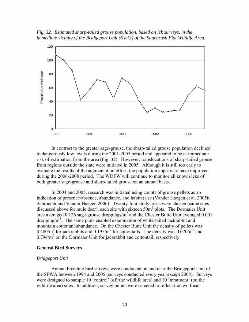
70
Fig. 32. Estimated sharp-tailed grouse population, based on lek surveys, in the immediate vicinity of the Bridgeport Unit (6 leks) of the Sagebrush Flat Wildlife Area.
0
20
40
60
80
100
120
1990 1994 1998 2002 2006
Popu
latio
n es
timat
e
In contrast to the greater sage-grouse, the sharp-tailed grouse population declined to dangerously low levels during the 2001-2005 period and appeared to be at immediate risk of extirpation from the area (Fig. 32). However, translocations of sharp-tailed grouse from regions outside the state were initiated in 2005. Although it is still too early to evaluate the results of the augmentation effort, the population appears to have improved during the 2006-2008 period. The WDFW will continue to monitor all known leks of both greater sage-grouse and sharp-tailed grouse on an annual basis.
In 2004 and 2005, research was initiated using counts of grouse pellets as an indication of presence/absence, abundance, and habitat use (Vander Haegen et al. 2005b, Schroeder and Vander Haegen 2006). Twenty-four study areas were chosen (same sites discussed above for mule deer), each site with sixteen 50m2 plots. The Dormaier Unit area averaged 0.126 sage-grouse droppings/m2 and the Chester Butte Unit averaged 0.001 dropping/m2. The same plots enabled examination of white-tailed jackrabbit and mountain cottontail abundance. On the Chester Butte Unit the density of pellets was 0.480/m2 for jackrabbits and 0.195/m2 for cottontails. The density was 0.070/m2 and 0.794/m2 on the Dormaier Unit for jackrabbit and cottontail, respectively.
General Bird Surveys
Bridgeport Unit
Annual breeding bird surveys were conducted on and near the Bridgeport Unit of the SFWA between 1994 and 2005 (surveys conducted every year except 2004). Surveys were designed to sample 10 ‘control’ (off the wildlife area) and 10 ‘treatment’ (on the wildlife area) sites. In addition, survey points were selected to reflect the two focal
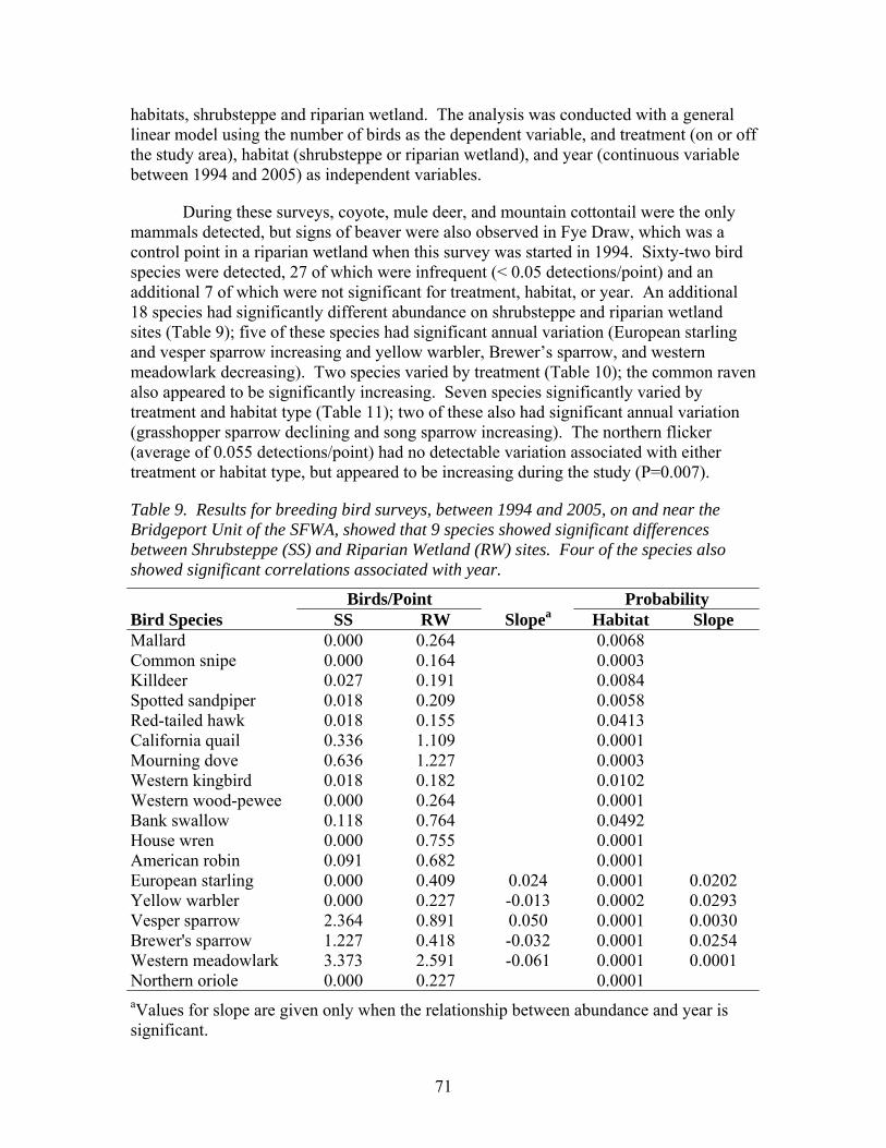
71
habitats, shrubsteppe and riparian wetland. The analysis was conducted with a general linear model using the number of birds as the dependent variable, and treatment (on or off the study area), habitat (shrubsteppe or riparian wetland), and year (continuous variable between 1994 and 2005) as independent variables.
During these surveys, coyote, mule deer, and mountain cottontail were the only mammals detected, but signs of beaver were also observed in Fye Draw, which was a control point in a riparian wetland when this survey was started in 1994. Sixty-two bird species were detected, 27 of which were infrequent (< 0.05 detections/point) and an additional 7 of which were not significant for treatment, habitat, or year. An additional 18 species had significantly different abundance on shrubsteppe and riparian wetland sites (Table 9); five of these species had significant annual variation (European starling and vesper sparrow increasing and yellow warbler, Brewer’s sparrow, and western meadowlark decreasing). Two species varied by treatment (Table 10); the common raven also appeared to be significantly increasing. Seven species significantly varied by treatment and habitat type (Table 11); two of these also had significant annual variation (grasshopper sparrow declining and song sparrow increasing). The northern flicker (average of 0.055 detections/point) had no detectable variation associated with either treatment or habitat type, but appeared to be increasing during the study (P=0.007).
Table 9. Results for breeding bird surveys, between 1994 and 2005, on and near the Bridgeport Unit of the SFWA, showed that 9 species showed significant differences between Shrubsteppe (SS) and Riparian Wetland (RW) sites. Four of the species also showed significant correlations associated with year.
Birds/Point Probability Bird Species SS RW Slopea Habitat Slope Mallard 0.000 0.264 0.0068 Common snipe 0.000 0.164 0.0003 Killdeer 0.027 0.191 0.0084 Spotted sandpiper 0.018 0.209 0.0058 Red-tailed hawk 0.018 0.155 0.0413 California quail 0.336 1.109 0.0001 Mourning dove 0.636 1.227 0.0003 Western kingbird 0.018 0.182 0.0102 Western wood-pewee 0.000 0.264 0.0001 Bank swallow 0.118 0.764 0.0492 House wren 0.000 0.755 0.0001 American robin 0.091 0.682 0.0001 European starling 0.000 0.409 0.024 0.0001 0.0202 Yellow warbler 0.000 0.227 -0.013 0.0002 0.0293 Vesper sparrow 2.364 0.891 0.050 0.0001 0.0030 Brewer's sparrow 1.227 0.418 -0.032 0.0001 0.0254 Western meadowlark 3.373 2.591 -0.061 0.0001 0.0001 Northern oriole 0.000 0.227 0.0001 aValues for slope are given only when the relationship between abundance and year is significant.
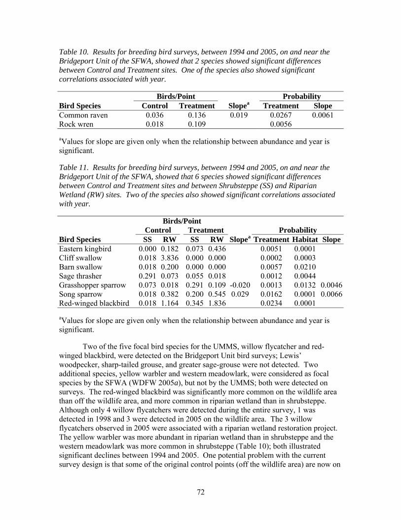
72
Table 10. Results for breeding bird surveys, between 1994 and 2005, on and near the Bridgeport Unit of the SFWA, showed that 2 species showed significant differences between Control and Treatment sites. One of the species also showed significant correlations associated with year.
Birds/Point Probability Bird Species Control Treatment Slopea Treatment Slope Common raven 0.036 0.136 0.019 0.0267 0.0061 Rock wren 0.018 0.109 0.0056
aValues for slope are given only when the relationship between abundance and year is significant.
Table 11. Results for breeding bird surveys, between 1994 and 2005, on and near the Bridgeport Unit of the SFWA, showed that 6 species showed significant differences between Control and Treatment sites and between Shrubsteppe (SS) and Riparian Wetland (RW) sites. Two of the species also showed significant correlations associated with year.
Birds/Point Control Treatment Probability Bird Species SS RW SS RW Slopea Treatment Habitat SlopeEastern kingbird 0.000 0.182 0.073 0.436 0.0051 0.0001 Cliff swallow 0.018 3.836 0.000 0.000 0.0002 0.0003 Barn swallow 0.018 0.200 0.000 0.000 0.0057 0.0210 Sage thrasher 0.291 0.073 0.055 0.018 0.0012 0.0044 Grasshopper sparrow 0.073 0.018 0.291 0.109 -0.020 0.0013 0.0132 0.0046Song sparrow 0.018 0.382 0.200 0.545 0.029 0.0162 0.0001 0.0066Red-winged blackbird 0.018 1.164 0.345 1.836 0.0234 0.0001
aValues for slope are given only when the relationship between abundance and year is significant.
Two of the five focal bird species for the UMMS, willow flycatcher and red-winged blackbird, were detected on the Bridgeport Unit bird surveys; Lewis’ woodpecker, sharp-tailed grouse, and greater sage-grouse were not detected. Two additional species, yellow warbler and western meadowlark, were considered as focal species by the SFWA (WDFW 2005a), but not by the UMMS; both were detected on surveys. The red-winged blackbird was significantly more common on the wildlife area than off the wildlife area, and more common in riparian wetland than in shrubsteppe. Although only 4 willow flycatchers were detected during the entire survey, 1 was detected in 1998 and 3 were detected in 2005 on the wildlife area. The 3 willow flycatchers observed in 2005 were associated with a riparian wetland restoration project. The yellow warbler was more abundant in riparian wetland than in shrubsteppe and the western meadowlark was more common in shrubsteppe (Table 10); both illustrated significant declines between 1994 and 2005. One potential problem with the current survey design is that some of the original control points (off the wildlife area) are now on
73
the wildlife area because of a recent acquisition. It will be important to re-evaluate the survey, and perhaps to potentially add some control points.
Results for the breeding bird surveys on the Bridgeport Unit were examined within each of the two focal habitats to evaluate relationships between species. Five species were significantly more abundant in shrubsteppe than in riparian wetland habitats including vesper sparrow, Brewer’s sparrow, western meadowlark, sage thrasher, and grasshopper sparrow; four of these species showed significant trends between 1994 and 2005 (grasshopper sparrow, Brewer’s sparrow, and western meadowlark were down and vesper sparrow was up). Although none was considered a focal species within the UMMS, the western meadowlark was considered a focal species on the SFWA. In addition, the sage thrasher, grasshopper sparrow, Brewer’s sparrow, and western meadowlark were often considered focal species in other subbasins and wildlife areas (Table 2). Many species were more common in riparian wetlands including: mallard, sora, American coot, common snipe, killdeer, spotted sandpiper, red-tailed hawk, California quail, mourning dove, eastern kingbird. western kingbird. western wood-pewee, bank swallow, cliff swallow, barn swallow, house wren, marsh wren, American robin, European starling, yellow warbler, song sparrow, and red-winged blackbird (regardless of sample size issues). Three of these species illustrated significant trends between 1994 and 2005; the European starling and song sparrow were increasing and the yellow warbler was decreasing.
Audubon-sponsored Christmas Bird Counts were conducted near Bridgeport starting in 1996. These counts completely included the Bridgeport Unit of the SFWA. The vast majority of the 141 species and the annual average of 21,000 birds were associated with the Columbia River and the habitats close to the river. Nevertheless, the Bridgeport Unit of the SFWA was characterized by many raptors (golden eagle, bald eagle, northern harrier, red-tailed hawk, rough-legged hawk, American kestrel, Cooper’s hawk, sharp-shinned hawk, prairie falcon, and northern goshawk. In addition great-horned owl, short-eared owl, sharp-tailed grouse, chukar, gray partridge, ring-necked pheasant, and many riparian wetland birds were observed. Most of the typical shrubsteppe birds, other than the horned lark, were not present because they had migrated off their breeding range. No attempt was made to evaluate trends.
Dormaier and Chester Butte Units
Breeding birds were examined in the Dormaier and Chester Butte units as part of research on shrubsteppe restoration between 2003 and 2005 (Vander Haegen et al. 2005a, 2005b). Forty-eight study areas were examined throughout north-central Washington in shrubsteppe and CRP habitats (Fig. 26). One study area was placed in the Dormaier Unit and one was placed in the Chester Butte Unit; each study area had 4 points that were used for surveys of breeding birds. Each of the study areas was surveyed twice each year.
The western meadowlark, vesper sparrow, Brewer’s sparrow, sage thrasher, mourning dove, and horned lark were the six most common species on the study sites. The ring-necked pheasant, California quail, savannah sparrow, Brewer’s sparrow, sage sparrow, western meadowlark, and brown-headed cowbird had significant variation
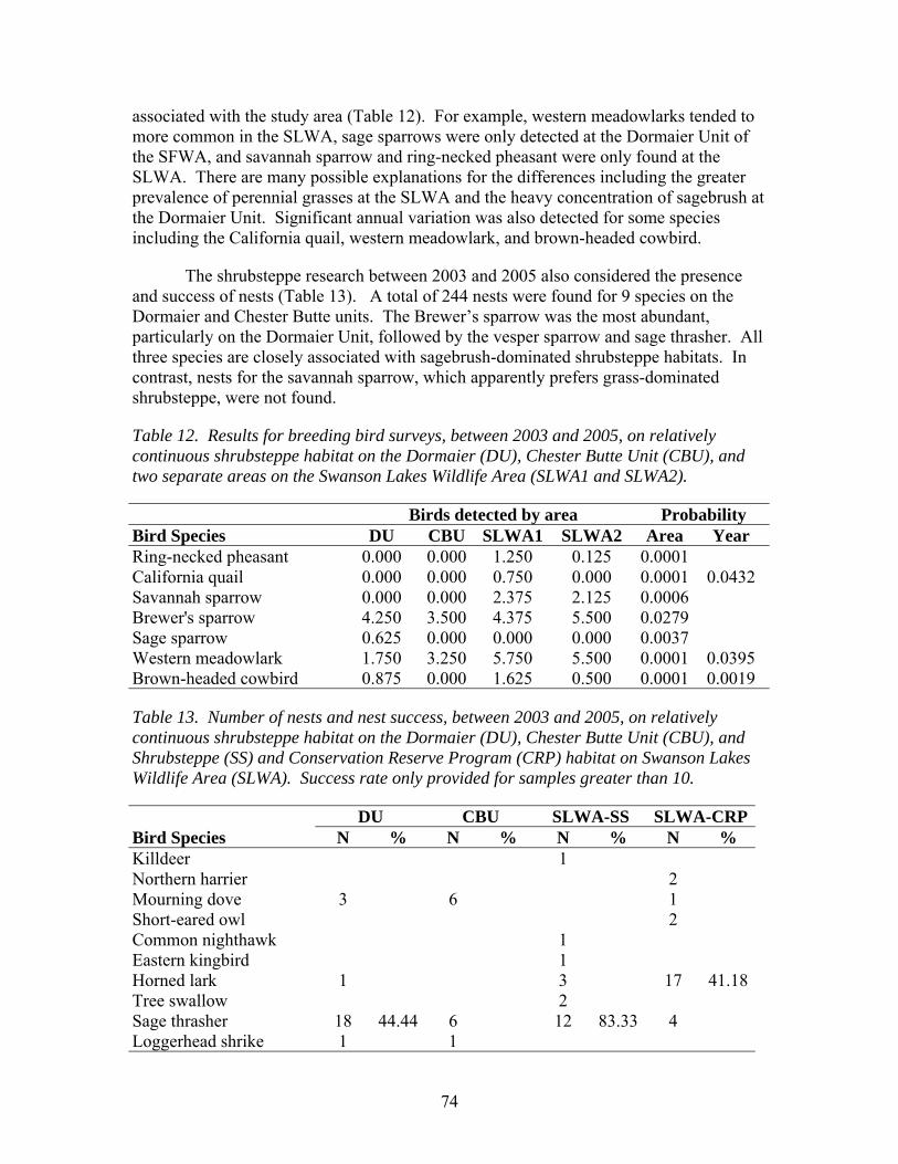
74
associated with the study area (Table 12). For example, western meadowlarks tended to more common in the SLWA, sage sparrows were only detected at the Dormaier Unit of the SFWA, and savannah sparrow and ring-necked pheasant were only found at the SLWA. There are many possible explanations for the differences including the greater prevalence of perennial grasses at the SLWA and the heavy concentration of sagebrush at the Dormaier Unit. Significant annual variation was also detected for some species including the California quail, western meadowlark, and brown-headed cowbird.
The shrubsteppe research between 2003 and 2005 also considered the presence and success of nests (Table 13). A total of 244 nests were found for 9 species on the Dormaier and Chester Butte units. The Brewer’s sparrow was the most abundant, particularly on the Dormaier Unit, followed by the vesper sparrow and sage thrasher. All three species are closely associated with sagebrush-dominated shrubsteppe habitats. In contrast, nests for the savannah sparrow, which apparently prefers grass-dominated shrubsteppe, were not found.
Table 12. Results for breeding bird surveys, between 2003 and 2005, on relatively continuous shrubsteppe habitat on the Dormaier (DU), Chester Butte Unit (CBU), and two separate areas on the Swanson Lakes Wildlife Area (SLWA1 and SLWA2).
Birds detected by area Probability Bird Species DU CBU SLWA1 SLWA2 Area Year Ring-necked pheasant 0.000 0.000 1.250 0.125 0.0001 California quail 0.000 0.000 0.750 0.000 0.0001 0.0432 Savannah sparrow 0.000 0.000 2.375 2.125 0.0006 Brewer's sparrow 4.250 3.500 4.375 5.500 0.0279 Sage sparrow 0.625 0.000 0.000 0.000 0.0037 Western meadowlark 1.750 3.250 5.750 5.500 0.0001 0.0395 Brown-headed cowbird 0.875 0.000 1.625 0.500 0.0001 0.0019
Table 13. Number of nests and nest success, between 2003 and 2005, on relatively continuous shrubsteppe habitat on the Dormaier (DU), Chester Butte Unit (CBU), and Shrubsteppe (SS) and Conservation Reserve Program (CRP) habitat on Swanson Lakes Wildlife Area (SLWA). Success rate only provided for samples greater than 10.
DU CBU SLWA-SS SLWA-CRPBird Species N % N % N % N % Killdeer 1 Northern harrier 2 Mourning dove 3 6 1 Short-eared owl 2 Common nighthawk 1 Eastern kingbird 1 Horned lark 1 3 17 41.18Tree swallow 2 Sage thrasher 18 44.44 6 12 83.33 4 Loggerhead shrike 1 1
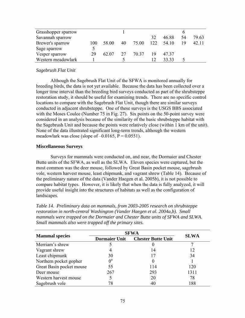
75
Grasshopper sparrow 1 6 Savannah sparrow 32 46.88 54 79.63Brewer's sparrow 100 58.00 40 75.00 122 54.10 19 42.11Sage sparrow 5 Vesper sparrow 29 62.07 27 70.37 19 47.37 Western meadowlark 1 5 12 33.33 5
Sagebrush Flat Unit
Although the Sagebrush Flat Unit of the SFWA is monitored annually for breeding birds, the data is not yet available. Because the data has been collected over a longer time interval than the breeding bird surveys conducted as part of the shrubsteppe restoration study, it should be useful for examining trends. There are no specific control locations to compare with the Sagebrush Flat Unit, though there are similar surveys conducted in adjacent shrubsteppe. One of these surveys is the USGS BBS associated with the Moses Coulee (Number 75 in Fig. 27). Six points on the 50-point survey were considered in an analysis because of the similarity of the basic shrubsteppe habitat with the Sagebrush Unit and because the points were relatively close (within 1 km of the unit). None of the data illustrated significant long-term trends, although the western meadowlark was close (slope of –0.0165, P = 0.0551).
Miscellaneous Surveys
Surveys for mammals were conducted on, and near, the Dormaier and Chester Butte units of the SFWA, as well as the SLWA. Eleven species were captured, but the most common was the deer mouse, followed by Great Basin pocket mouse, sagebrush vole, western harvest mouse, least chipmunk, and vagrant shrew (Table 14). Because of the preliminary nature of the data (Vander Haegen et al. 2005b), it is not possible to compare habitat types. However, it is likely that when the data is fully analyzed, it will provide useful insight into the structures of habitats as well as the configuration of landscapes.
Table 14. Preliminary data on mammals, from 2003-2005 research on shrubsteppe restoration in north-central Washington (Vander Haegen et al. 2004a,b). Small mammals were trapped on the Dormaier and Chester Butte units of SFWA and SLWA. Small mammals also were trapped off the primary sites.
SFWA Mammal species Dormaier Unit Chester Butte Unit SLWA
Merriam’s shrew 5 0 7 Vagrant shrew 4 14 12 Least chipmunk 30 17 34 Northern pocket gopher 0a 0 1 Great Basin pocket mouse 55 114 120 Deer mouse 267 293 1311 Western harvest mouse 5 20 78 Sagebrush vole 78 40 188
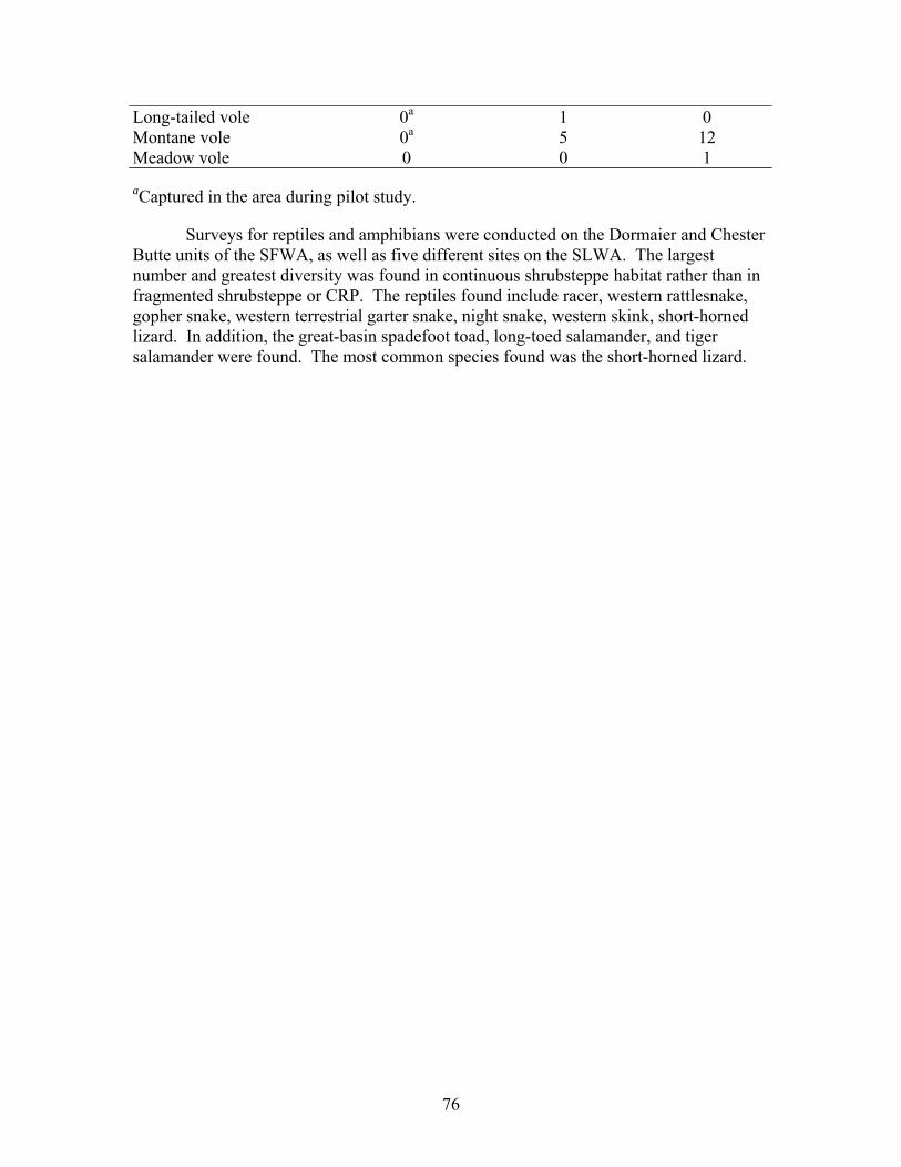
76
Long-tailed vole 0a 1 0 Montane vole 0a 5 12 Meadow vole 0 0 1
aCaptured in the area during pilot study.
Surveys for reptiles and amphibians were conducted on the Dormaier and Chester Butte units of the SFWA, as well as five different sites on the SLWA. The largest number and greatest diversity was found in continuous shrubsteppe habitat rather than in fragmented shrubsteppe or CRP. The reptiles found include racer, western rattlesnake, gopher snake, western terrestrial garter snake, night snake, western skink, short-horned lizard. In addition, the great-basin spadefoot toad, long-toed salamander, and tiger salamander were found. The most common species found was the short-horned lizard.
77
SCOTCH CREEK WILDLIFE AREA
DESCRIPTION
Acquisition of the SCWA began in 1991 with the purchase of the Metcalf Ranch near Conconully, Washington to permanently protect Sharp-tailed grouse and shrubsteppe habitat (WDFW 2005b). Since the initial acquisition, addition purchases have expanded the property boundaries. The SCWA now consist of 5 separate units in North Central Washington (WDFW 2005b; Fig. 33); Scotch Creek, Mineral Hill, Pogue Mountain, Tunk Valley, and Chesaw. All units but the Chesaw Unit are in the OKS (NPPC 2004d); the Chesaw Unit is within the UCS (NPPC 2004e).
The 3,518-ha Scotch Creek unit consists of 1,719 ha of shrub-dominated shrubsteppe (> 15% shrub cover), 1,503 ha of grass-dominated shrubsteppe (< 15% shrub cover), 211 ha of conifer forest, 32 ha maintained in agricultural (sharecrop fields), 30 ha riparian, and 23 ha in surface water. The Scotch Creek Unit supports the core of the sharp-tailed grouse population on the SCWA. The 372-ha Mineral Hill Unit consists of 247 ha conifer forest, 102 has of grass-dominated shrubsteppe, and 23 ha of riparian Forest. It is along the West Fork of Salmon Creek. A natural waterfall barrier downstream from this property prevents anadromous fish from utilizing this stream. The 484-ha Pogue Mountain Unit consists of 291 ha of shrubsteppe, 192 ha of conifer forest, and 1 ha of surface water. The unit is managed as mule deer winter range, however there are historical accounts of sharp-tailed grouse use on the lower elevations. The 566-ha Tunk Valley Unit consists of shrubsteppe with a small amount of forest. The area also supports a variety of species including mule deer, white-tailed deer, sharp-tailed grouse, ruffed grouse, California quail, and gray partridge. The 1,745-ha Chesaw Unit consists of 882 ha of grass-dominated shrubsteppe, 608 ha of shrub-dominated shrubsteppe, 181 ha of conifer forest, 58 ha of riparian wetland, and 16 ha of surface water. The area supports sharp-tailed grouse as well as mule deer, white-tailed deer, ruffed grouse, and blue (dusky) grouse.
In 1997, the BPA accepted management responsibilities to mitigate for losses resulting from the construction of Grand Coulee and Chief Joseph hydroelectric dams (Table 1). These losses include sharp-tailed grouse (35,013 HUs), mule deer (29,125 HUs), white-tailed deer (21,362 HUs), Lewis woodpecker (286 HUs), and mourning dove (9,316 HUs) (NPPC 2000).
Management goals for the SCWA are to preserve habitat and species diversity for wildlife resources, maintain healthy populations of game and non-game species, protect and restore native plant communities, and provide diverse opportunities for the public to encounter, utilize, and appreciate wildlife and wild areas (WDFW 2005b). Although the SCWA is primarily managed to promote recovery of the sharp-tailed grouse, management is also directed toward the protection and management of other shrubsteppe obligate species (WDFW 2005b). Some of these specific wildlife objectives are listed below:
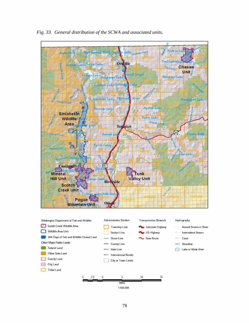
78
Fig. 33. General distribution of the SCWA and associated units.
79
1. Preserve, protect, perpetuate, and manage deer and their habitat to ensure healthy, productive, and sustainable populations. Strategies for this broad objective include: 1) Conduct prescribed fuels treatments including logging and prescribed fire; 2) Acquire conservation easements to provide long-term protection of critical habitat; 3) Use well-managed livestock grazing where appropriate as a tool to improve habitat; and 4) Seed or plant bitterbrush in burned and/or disturbed areas.
2. Identify, improve, and maintain fish populations along Scotch Creek, West Fork Salmon Creek, Tunk Creek, and Mary Ann Creek.
3. Manage upland birds and their habitats, in particular sharp-tailed grouse and the shrubsteppe and riparian wetland habitats upon which they depend. Strategies include: 1) Avoid accidental harvest of sharp-tailed grouse by hunters of other upland birds (ring-neck pheasants, gray partridge, chukar, California quail, blue grouse); 2) Maintain springs and guzzlers to provide water for upland birds and other species; 3) Restore and protect the shrubsteppe and riparian wetlands upon which sharp-tailed grouse depend.
4. Develop and maintain quality habitat that will provide life requisites for a diversity of species. Nearly all activities on the wildlife area benefit a diversity of species. Strategies include: 1) performing surveys for breeding birds, amphibians, mammals, and reptiles; 2) Assess timber-thinning projects to reduce potential insect and catastrophic fire danger and create forest conditions more suitable to a diversity of species; and 3) Cooperate with agencies and non-governmental groups to acquire information on wildlife use of the area.
5. Protect and restore riparian habitat. The agency has prioritized riparian habitat management and protection. Riparian areas provide habitat for a large diversity of fish and wildlife species, high densities of animals, important breeding areas, and movement corridors. Strategies include: 1) Restore stretch of Scotch Creek to mimic a natural stream corridor (low gradient) with a wide, narrow, and deep meandering channel and replanted riparian vegetation; and 2) In areas permitted for grazing by domestic livestock on Chesaw and Scotch Creek, fence riparian habitats to protect them from unmanaged grazing impacts.
6. Protect and restore shrubsteppe habitat. The SCWA has the highest priority to protect and enhance shrubsteppe habitat. The agency has also prioritized shrubsteppe habitat management and protection. Shrubsteppe areas provide habitat for a diversity of fish and wildlife species and for comparatively high densities of animals. Shrubsteppe is also very vulnerable to habitat conversion and alteration practices. Over the past 14 years (since acquisition) all units of the SCWA have undergone native shrubsteppe restoration. Over 1,000 ha have been restored from an
80
agricultural field composition to a diverse mix of native grasses and forbs. Additional strategies include: 1) Perform shrubsteppe condition surveys to assess habitat quality issues; 2) Continue to restore old agriculture fields to native shrubsteppe habitat at the rate of 100 acres per year for the next 5 years; 3) Conduct, with the cooperation of the DNR and other fire districts, prescribed fire on the shrubsteppe habitat of the Tunk Valley unit to promote a higher cover of herbaceous plants and create a mosaic of woody species to increase overall diversity; 4) Collect seeds of native plant species on the SCWA to have commercially grown to provide a large quantity of locally adapted seed stock for restoration purposes; 5) Evaluate and use prescribed fires on all areas where appropriate to rejuvenate and improve shrub-steppe habitat and reduce the risk of catastrophic fires; and 6) Manage weeds consistent with state and county rules and to protect and recover fish and wildlife and their habitats.
7. Protect and manage other species dependent on high quality shrubsteppe, forest, and riparian habitat conditions to enhance obligate species protection. Strategies include: 1) Protection and creation of nesting and foraging habitat for several woodpecker species; and 2) Expansion and maintenance of nest boxes.
8. Manage species and habitats in compliance with the ESA and Washington State fish passage, road management and forest practice rules. Strategies include: 1) Protection of buffers adjacent to wetlands and riparian habitat; 2) Identify fish passage structures and sedimentation issues; 3) Map all ESA species and their habitats on the SCWA and address relevant management practices.
UPPER MIDDLE MAINSTEM AND UPPER COLUMBIA SUBBASINS
The NPPC (2004e) recommends specific strategies to address habitat and biological objectives in three focal habitats; shrubsteppe, riparian wetland, and Ponderosa pine. While all habitats are important, these focal habitats were selected in part because they are disproportionately vulnerable to anthropogenic impacts, and likely have received the highest level of impacts within the subbasin. Some of the identified impacts are, for all practical purposes, irreversible and others are already being mitigated through ongoing management. The NPPC (2004d) recommends consideration of the same three focal habitats, but in addition considers cliff/rock outcrop, and herbaceous wetland. However, because the Chesaw Unit only includes shrubsteppe, riparian wetland, and Ponderosa pine habitats, and because the Chesaw Unit was the only portion of the SCWA within the UCS, cliff/rock outcrop and herbaceous wetland were not considered here. The focal species considered here within these focal habitats included: 1) white-headed woodpecker, pygmy nuthatch, gray flycatcher, and flammulated owl in Ponderosa pine; 2) sharp-tailed grouse, greater sage-grouse, mule deer, Brewer’s sparrow, and grasshopper sparrow in shrubsteppe; and 3) red-eyed vireo, yellow-breasted chat, and American beaver in riparian wetlands.
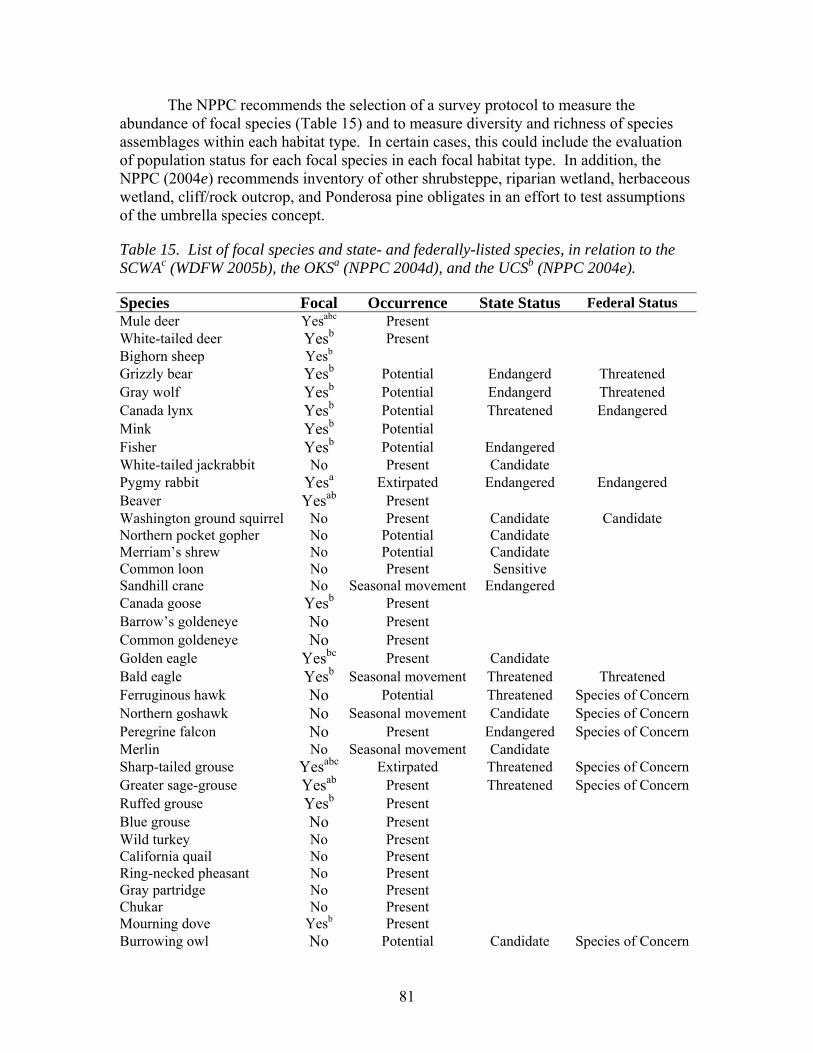
81
The NPPC recommends the selection of a survey protocol to measure the abundance of focal species (Table 15) and to measure diversity and richness of species assemblages within each habitat type. In certain cases, this could include the evaluation of population status for each focal species in each focal habitat type. In addition, the NPPC (2004e) recommends inventory of other shrubsteppe, riparian wetland, herbaceous wetland, cliff/rock outcrop, and Ponderosa pine obligates in an effort to test assumptions of the umbrella species concept.
Table 15. List of focal species and state- and federally-listed species, in relation to the SCWAc (WDFW 2005b), the OKSa (NPPC 2004d), and the UCSb (NPPC 2004e).
Species Focal Occurrence State Status Federal Status Mule deer Yesabc Present White-tailed deer Yesb Present Bighorn sheep Yesb Grizzly bear Yesb Potential Endangerd Threatened Gray wolf Yesb Potential Endangerd Threatened Canada lynx Yesb Potential Threatened Endangered Mink Yesb Potential Fisher Yesb Potential Endangered White-tailed jackrabbit No Present Candidate Pygmy rabbit Yesa Extirpated Endangered Endangered Beaver Yesab Present Washington ground squirrel No Present Candidate Candidate Northern pocket gopher No Potential Candidate Merriam’s shrew No Potential Candidate Common loon No Present Sensitive Sandhill crane No Seasonal movement Endangered Canada goose Yesb Present Barrow’s goldeneye No Present Common goldeneye No Present Golden eagle Yesbc Present Candidate Bald eagle Yesb Seasonal movement Threatened Threatened Ferruginous hawk No Potential Threatened Species of Concern Northern goshawk No Seasonal movement Candidate Species of Concern Peregrine falcon No Present Endangered Species of Concern Merlin No Seasonal movement Candidate Sharp-tailed grouse Yesabc Extirpated Threatened Species of Concern Greater sage-grouse Yesab Present Threatened Species of Concern Ruffed grouse Yesb Present Blue grouse No Present Wild turkey No Present California quail No Present Ring-necked pheasant No Present Gray partridge No Present Chukar No Present Mourning dove Yesb Present Burrowing owl No Potential Candidate Species of Concern
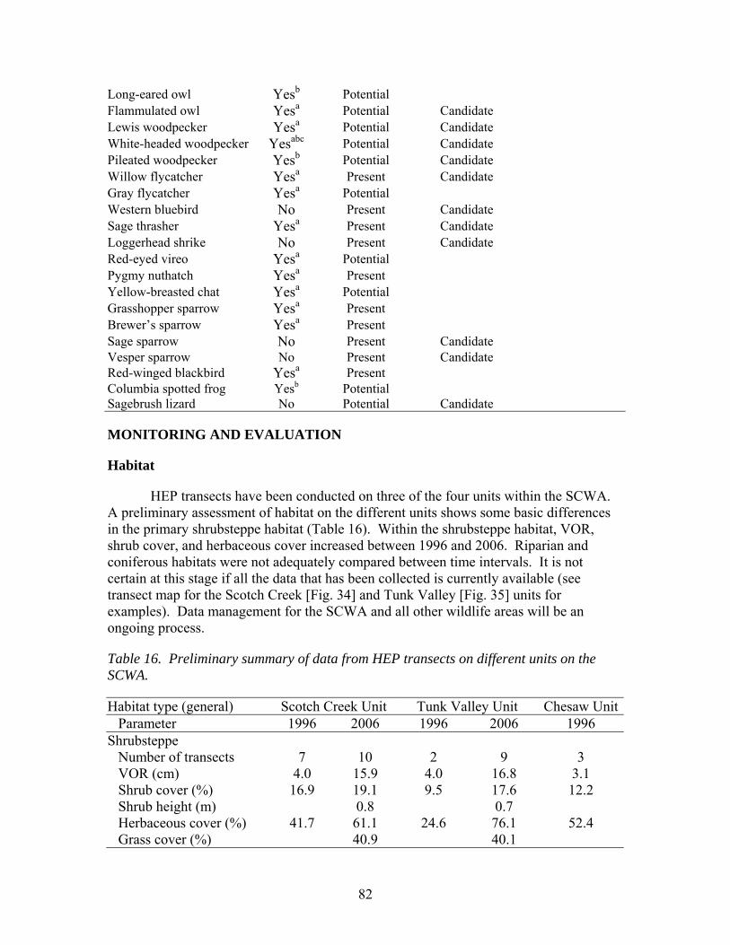
82
Long-eared owl Yesb Potential Flammulated owl Yesa Potential Candidate Lewis woodpecker Yesa Potential Candidate White-headed woodpecker Yesabc Potential Candidate Pileated woodpecker Yesb Potential Candidate Willow flycatcher Yesa Present Candidate Gray flycatcher Yesa Potential Western bluebird No Present Candidate Sage thrasher Yesa Present Candidate Loggerhead shrike No Present Candidate Red-eyed vireo Yesa Potential Pygmy nuthatch Yesa Present Yellow-breasted chat Yesa Potential Grasshopper sparrow Yesa Present Brewer’s sparrow Yesa Present Sage sparrow No Present Candidate Vesper sparrow No Present Candidate Red-winged blackbird Yesa Present Columbia spotted frog Yesb Potential Sagebrush lizard No Potential Candidate
MONITORING AND EVALUATION
Habitat
HEP transects have been conducted on three of the four units within the SCWA. A preliminary assessment of habitat on the different units shows some basic differences in the primary shrubsteppe habitat (Table 16). Within the shrubsteppe habitat, VOR, shrub cover, and herbaceous cover increased between 1996 and 2006. Riparian and coniferous habitats were not adequately compared between time intervals. It is not certain at this stage if all the data that has been collected is currently available (see transect map for the Scotch Creek [Fig. 34] and Tunk Valley [Fig. 35] units for examples). Data management for the SCWA and all other wildlife areas will be an ongoing process.
Table 16. Preliminary summary of data from HEP transects on different units on the SCWA.
Habitat type (general) Scotch Creek Unit Tunk Valley Unit Chesaw Unit Parameter 1996 2006 1996 2006 1996 Shrubsteppe Number of transects 7 10 2 9 3 VOR (cm) 4.0 15.9 4.0 16.8 3.1 Shrub cover (%) 16.9 19.1 9.5 17.6 12.2 Shrub height (m) 0.8 0.7 Herbaceous cover (%) 41.7 61.1 24.6 76.1 52.4 Grass cover (%) 40.9 40.1
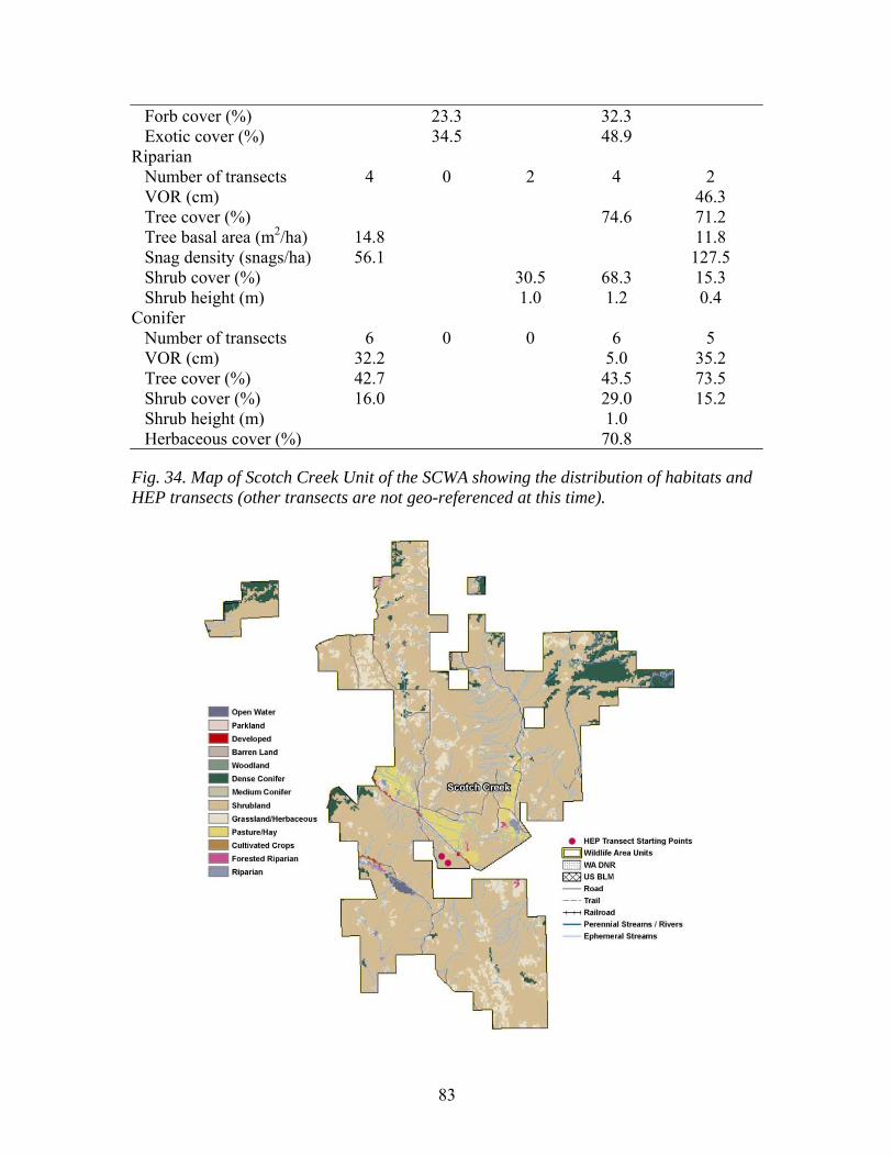
83
Forb cover (%) 23.3 32.3 Exotic cover (%) 34.5 48.9 Riparian Number of transects 4 0 2 4 2 VOR (cm) 46.3 Tree cover (%) 74.6 71.2 Tree basal area (m2/ha) 14.8 11.8 Snag density (snags/ha) 56.1 127.5 Shrub cover (%) 30.5 68.3 15.3 Shrub height (m) 1.0 1.2 0.4 Conifer Number of transects 6 0 0 6 5 VOR (cm) 32.2 5.0 35.2 Tree cover (%) 42.7 43.5 73.5 Shrub cover (%) 16.0 29.0 15.2 Shrub height (m) 1.0 Herbaceous cover (%) 70.8
Fig. 34. Map of Scotch Creek Unit of the SCWA showing the distribution of habitats and HEP transects (other transects are not geo-referenced at this time).
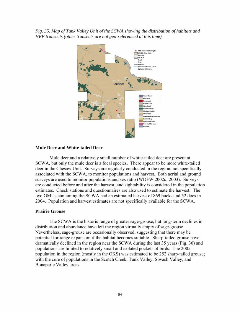
84
Fig. 35. Map of Tunk Valley Unit of the SCWA showing the distribution of habitats and HEP transects (other transects are not geo-referenced at this time).
Mule Deer and White-tailed Deer
Mule deer and a relatively small number of white-tailed deer are present at SCWA, but only the mule deer is a focal species. There appear to be more white-tailed deer in the Chesaw Unit. Surveys are regularly conducted in the region, not specifically associated with the SCWA, to monitor populations and harvest. Both aerial and ground surveys are used to monitor populations and sex ratio (WDFW 2002a, 2003). Surveys are conducted before and after the harvest, and sightability is considered in the population estimates. Check stations and questionnaires are also used to estimate the harvest. The two GMUs containing the SCWA had an estimated harvest of 869 bucks and 52 does in 2004. Population and harvest estimates are not specifically available for the SCWA.
Prairie Grouse
The SCWA is the historic range of greater sage-grouse, but long-term declines in distribution and abundance have left the region virtually empty of sage-grouse. Nevertheless, sage-grouse are occasionally observed, suggesting that there may be potential for range expansion if the habitat becomes suitable. Sharp-tailed grouse have dramatically declined in the region near the SCWA during the last 35 years (Fig. 36) and populations are limited to relatively small and isolated pockets of birds. The 2005 population in the region (mostly in the OKS) was estimated to be 252 sharp-tailed grouse; with the core of populations in the Scotch Creek, Tunk Valley, Siwash Valley, and Bonaparte Valley areas.
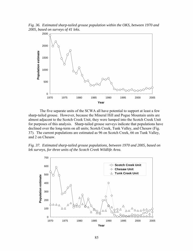
85
Fig. 36. Estimated sharp-tailed grouse population within the OKS, between 1970 and 2005, based on surveys of 41 leks.
0
500
1000
1500
2000
2500
1970 1975 1980 1985 1990 1995 2000 2005
Year
Popu
latio
n es
timat
e
The five separate units of the SCWA all have potential to support at least a few sharp-tailed grouse. However, because the Mineral Hill and Pogue Mountain units are almost adjacent to the Scotch Creek Unit, they were lumped into the Scotch Creek Unit for purposes of this analysis. Sharp-tailed grouse surveys indicate that populations have declined over the long-term on all units; Scotch Creek, Tunk Valley, and Chesaw (Fig. 37). The current populations are estimated as 96 on Scotch Creek, 66 on Tunk Valley, and 2 on Chesaw.
Fig. 37. Estimated sharp-tailed grouse populations, between 1970 and 2005, based on lek surveys, for three units of the Scotch Creek Wildlife Area.
0
100
200
300
400
500
600
700
1970 1975 1980 1985 1990 1995 2000 2005
Year
Popu
latio
n es
timat
e
Scotch Creek UnitChesaw UnitTunk Creek Unit

86
In the mid- and late 1990s the population declined so much on the Scotch Creek Unit, that sharp-tailed grouse were translocated from other populations (mostly from Idaho, but also from the Nespelem area in Washington) in an effort to augment the population. This was predicted to have beneficial effects on the genetics of birds in Washington as well as the demography of the ‘new’ mixed population. The population at the Scotch Creek Unit appears to have responded positively through an increase in the number of birds and the number of leks upon which they display (Fig. 38). There are now three sharp-tailed grouse leks on the Scotch Creek Unit and a single lek on the Chesaw Unit. There are leks near the Tunk Valley Unit, but there are not on the public land. The WDFW will continue to monitor all known leks of sharp-tailed grouse on an annual basis.
Fig. 38. Estimated sharp-tailed grouse population, before, during (triangles), and after translocation in the Scotch Creek Unit of the Scotch Creek Wildlife Area, 1978-2008.
0
50
100
150
200
250
300
1978 1983 1988 1993 1998 2003 2008
Popu
latio
n es
timat
e
Before translocation
During and after translocation
General Bird Surveys
Scotch Creek Unit
Annual breeding bird surveys were conducted on and near the Scotch Creek Unit of the SCWA between 1993 and 2005 (surveys conducted every year except 2004). Surveys were designed to sample ‘control’ (off the wildlife areas) and ‘treatment’ (on the wildlife area) sites. In addition, survey points were selected to reflect the two focal habitats, shrubsteppe and riparian wetland, as well as Honey Lake on the SCWA and Hess Lake off the SCWA. The analysis was conducted with a general linear model using the number of birds as the dependent variable, and treatment (on or off the study area), habitat (shrubsteppe or riparian wetland), and year (continuous variable between 1993 and 2005) as independent variables.
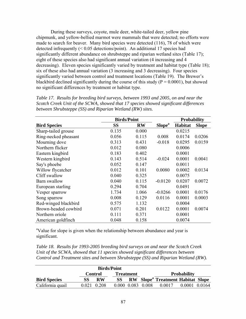
87
During these surveys, coyote, mule deer, white-tailed deer, yellow pine chipmunk, and yellow-bellied marmot were mammals that were detected; no efforts were made to search for beaver. Many bird species were detected (116), 78 of which were detected infrequently (< 0.05 detections/point). An additional 17 species had significantly different abundance on shrubsteppe and riparian wetland sites (Table 17); eight of these species also had significant annual variation (4 increasing and 4 decreasing). Eleven species significantly varied by treatment and habitat type (Table 18); six of these also had annual variation (3 increasing and 3 decreasing). Four species significantly varied between control and treatment locations (Table 19). The Brewer’s blackbird declined significantly during the course of this study (P = 0.0001), but showed no significant differences by treatment or habitat type.
Table 17. Results for breeding bird surveys, between 1993 and 2005, on and near the Scotch Creek Unit of the SCWA, showed that 17 species showed significant differences between Shrubsteppe (SS) and Riparian Wetland (RW) sites.
Birds/Point Probability Bird Species SS RW Slopea Habitat Slope Sharp-tailed grouse 0.135 0.000 0.0215 Ring-necked pheasant 0.056 0.115 0.008 0.0174 0.0206 Mourning dove 0.313 0.431 -0.018 0.0295 0.0159 Northern flicker 0.012 0.080 0.0006 Eastern kingbird 0.183 0.402 0.0001 Western kingbird 0.143 0.514 -0.024 0.0001 0.0041 Say's phoebe 0.052 0.147 0.0011 Willow flycatcher 0.012 0.101 0.0080 0.0002 0.0134 Cliff swallow 0.040 0.325 0.0075 Barn swallow 0.040 0.115 -0.0120 0.0207 0.0072 European starling 0.294 0.704 0.0491 Vesper sparrow 1.734 1.066 -0.0266 0.0001 0.0176 Song sparrow 0.008 0.129 0.0116 0.0001 0.0003 Red-winged blackbird 0.575 1.132 0.0004 Brown-headed cowbird 0.071 0.201 0.0122 0.0001 0.0074 Northern oriole 0.111 0.371 0.0001 American goldfinch 0.048 0.158 0.0074
aValue for slope is given when the relationship between abundance and year is significant.
Table 18. Results for 1993-2005 breeding bird surveys on and near the Scotch Creek Unit of the SCWA, showed that 11 species showed significant differences between Control and Treatment sites and between Shrubsteppe (SS) and Riparian Wetland (RW).
Birds/Point Control Treatment Probability Bird Species SS RW SS RW Slopea Treatment Habitat SlopeCalifornia quail 0.021 0.208 0.000 0.083 0.008 0.0017 0.0001 0.0164
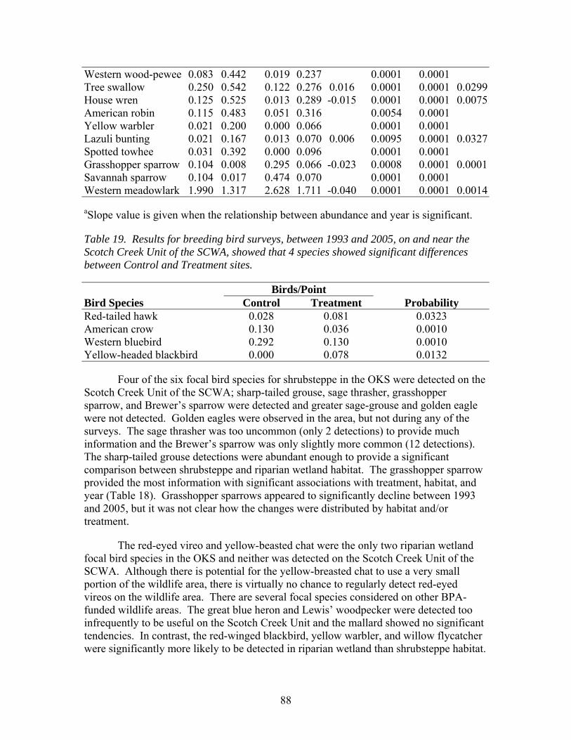
88
Western wood-pewee 0.083 0.442 0.019 0.237 0.0001 0.0001 Tree swallow 0.250 0.542 0.122 0.276 0.016 0.0001 0.0001 0.0299House wren 0.125 0.525 0.013 0.289 -0.015 0.0001 0.0001 0.0075American robin 0.115 0.483 0.051 0.316 0.0054 0.0001 Yellow warbler 0.021 0.200 0.000 0.066 0.0001 0.0001 Lazuli bunting 0.021 0.167 0.013 0.070 0.006 0.0095 0.0001 0.0327Spotted towhee 0.031 0.392 0.000 0.096 0.0001 0.0001 Grasshopper sparrow 0.104 0.008 0.295 0.066 -0.023 0.0008 0.0001 0.0001Savannah sparrow 0.104 0.017 0.474 0.070 0.0001 0.0001 Western meadowlark 1.990 1.317 2.628 1.711 -0.040 0.0001 0.0001 0.0014
aSlope value is given when the relationship between abundance and year is significant.
Table 19. Results for breeding bird surveys, between 1993 and 2005, on and near the Scotch Creek Unit of the SCWA, showed that 4 species showed significant differences between Control and Treatment sites.
Birds/Point Bird Species Control Treatment Probability Red-tailed hawk 0.028 0.081 0.0323 American crow 0.130 0.036 0.0010 Western bluebird 0.292 0.130 0.0010 Yellow-headed blackbird 0.000 0.078 0.0132
Four of the six focal bird species for shrubsteppe in the OKS were detected on the Scotch Creek Unit of the SCWA; sharp-tailed grouse, sage thrasher, grasshopper sparrow, and Brewer’s sparrow were detected and greater sage-grouse and golden eagle were not detected. Golden eagles were observed in the area, but not during any of the surveys. The sage thrasher was too uncommon (only 2 detections) to provide much information and the Brewer’s sparrow was only slightly more common (12 detections). The sharp-tailed grouse detections were abundant enough to provide a significant comparison between shrubsteppe and riparian wetland habitat. The grasshopper sparrow provided the most information with significant associations with treatment, habitat, and year (Table 18). Grasshopper sparrows appeared to significantly decline between 1993 and 2005, but it was not clear how the changes were distributed by habitat and/or treatment.
The red-eyed vireo and yellow-beasted chat were the only two riparian wetland focal bird species in the OKS and neither was detected on the Scotch Creek Unit of the SCWA. Although there is potential for the yellow-breasted chat to use a very small portion of the wildlife area, there is virtually no chance to regularly detect red-eyed vireos on the wildlife area. There are several focal species considered on other BPA-funded wildlife areas. The great blue heron and Lewis’ woodpecker were detected too infrequently to be useful on the Scotch Creek Unit and the mallard showed no significant tendencies. In contrast, the red-winged blackbird, yellow warbler, and willow flycatcher were significantly more likely to be detected in riparian wetland than shrubsteppe habitat.
89
In addition the willow flycatcher significantly increased between 1993 and 2005 (Table 17).
Results for the breeding bird surveys on the Scotch Creek Unit were examined within each of the two focal habitats to evaluate relationships between species. Seven species were significantly more abundant in shrubsteppe than in riparian wetland habitats including sharp-tailed grouse, gray partridge, short-eared owl, grasshopper sparrow, vesper sparrow, savannah sparrow, and western meadowlark (regardless of sample size issues); three of these species showed significant downward trends between 1993 and 2005 (grasshopper sparrow, vesper sparrow, and western meadowlark). The sharp-tailed grouse and grasshopper sparrow were both considered focal species within the OKS. Thirty-two species were more common in riparian wetlands than in shrubsteppe habitats. Seven of these species (California quail, ring-necked pheasant, willow flycatcher, tree swallow, Lazuli bunting, song sparrow, and brown-headed cowbird) significantly increased between 1993 and 2005. Four of these species (mourning dove, western kingbird, barn swallow, and house wren) significantly decreased. None is considered a focal species in the OKS, though the willow flycatcher is a focal species in the UMMS.
Seventy-six species were observed on the Omak Christmas Bird Count during 2002-2004. The most common species observed were, in order of abundance: California quail, Canada goose, European starling, dark-eyed junco, house sparrow, mallard, house finch, and rock pigeon. None of the common birds appeared to be the characteristic birds of shrubsteppe, riparian wetland, and Ponderosa pine. Black-capped chickadee, mourning dove, red-winged blackbird, white-crowned sparrow, pygmy nuthatch, American tree sparrow, and blue grouse were observed, but in low numbers.
Chesaw Unit
Annual breeding bird surveys were conducted on and near the Chesaw Unit of the SCWA between 1993 and 2005 (surveys conducted every year except 2004). Surveys were designed to sample ‘control’ (off the wildlife areas) and ‘treatment’ (on the wildlife area) sites. In addition, survey points were selected to reflect the two focal habitats, shrubsteppe and riparian wetland, as well as small lakes on and off the Chesaw Unit. The analysis was conducted with a general linear model using the number of birds as the dependent variable, and treatment (on or off the study area), habitat (shrubsteppe or riparian wetland), and year (continuous variable between 1993 and 2005) as independent variables. Although birds observed at lakes were not considered in the statistical analysis, different species of birds that were detected at the lakes, but not found elsewhere, were recorded.
During these surveys muskrat, American beaver, coyote, mule deer, white-tailed deer, elk, yellow pine chipmunk, red squirrel, yellow-bellied marmot, and Columbian ground squirrel were mammals that were detected. Many bird species were detected (113), 71 of which were detected infrequently (< 0.05 detections/point). An additional 10 species had significantly different abundance on shrubsteppe and riparian wetland sites (Table 20); four of these species also had significant annual variation (1 increasing and 3 decreasing). Five species significantly varied between control and treatment locations
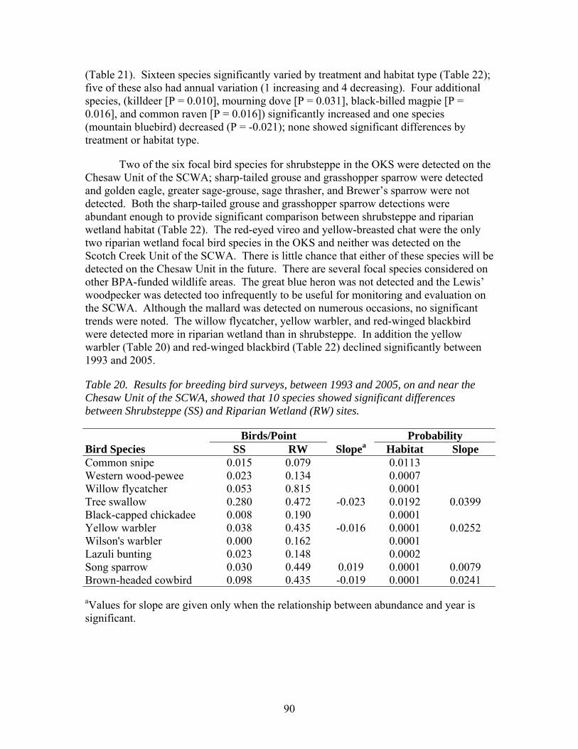
90
(Table 21). Sixteen species significantly varied by treatment and habitat type (Table 22); five of these also had annual variation (1 increasing and 4 decreasing). Four additional species, (killdeer [P = 0.010], mourning dove [P = 0.031], black-billed magpie [P = 0.016], and common raven [P = 0.016]) significantly increased and one species (mountain bluebird) decreased (P = -0.021); none showed significant differences by treatment or habitat type.
Two of the six focal bird species for shrubsteppe in the OKS were detected on the Chesaw Unit of the SCWA; sharp-tailed grouse and grasshopper sparrow were detected and golden eagle, greater sage-grouse, sage thrasher, and Brewer’s sparrow were not detected. Both the sharp-tailed grouse and grasshopper sparrow detections were abundant enough to provide significant comparison between shrubsteppe and riparian wetland habitat (Table 22). The red-eyed vireo and yellow-breasted chat were the only two riparian wetland focal bird species in the OKS and neither was detected on the Scotch Creek Unit of the SCWA. There is little chance that either of these species will be detected on the Chesaw Unit in the future. There are several focal species considered on other BPA-funded wildlife areas. The great blue heron was not detected and the Lewis’ woodpecker was detected too infrequently to be useful for monitoring and evaluation on the SCWA. Although the mallard was detected on numerous occasions, no significant trends were noted. The willow flycatcher, yellow warbler, and red-winged blackbird were detected more in riparian wetland than in shrubsteppe. In addition the yellow warbler (Table 20) and red-winged blackbird (Table 22) declined significantly between 1993 and 2005.
Table 20. Results for breeding bird surveys, between 1993 and 2005, on and near the Chesaw Unit of the SCWA, showed that 10 species showed significant differences between Shrubsteppe (SS) and Riparian Wetland (RW) sites.
Birds/Point Probability Bird Species SS RW Slopea Habitat Slope Common snipe 0.015 0.079 0.0113 Western wood-pewee 0.023 0.134 0.0007 Willow flycatcher 0.053 0.815 0.0001 Tree swallow 0.280 0.472 -0.023 0.0192 0.0399 Black-capped chickadee 0.008 0.190 0.0001 Yellow warbler 0.038 0.435 -0.016 0.0001 0.0252 Wilson's warbler 0.000 0.162 0.0001 Lazuli bunting 0.023 0.148 0.0002 Song sparrow 0.030 0.449 0.019 0.0001 0.0079 Brown-headed cowbird 0.098 0.435 -0.019 0.0001 0.0241
aValues for slope are given only when the relationship between abundance and year is significant.
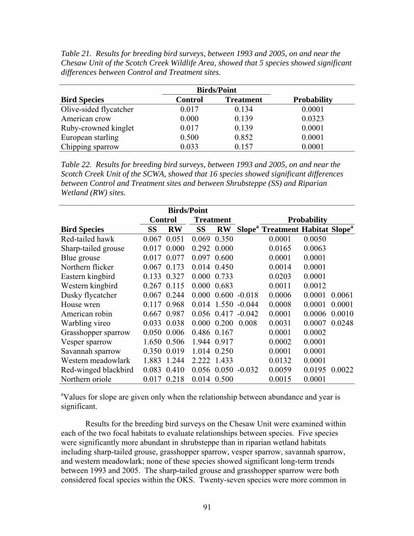
91
Table 21. Results for breeding bird surveys, between 1993 and 2005, on and near the Chesaw Unit of the Scotch Creek Wildlife Area, showed that 5 species showed significant differences between Control and Treatment sites.
Birds/Point Bird Species Control Treatment Probability Olive-sided flycatcher 0.017 0.134 0.0001 American crow 0.000 0.139 0.0323 Ruby-crowned kinglet 0.017 0.139 0.0001 European starling 0.500 0.852 0.0001 Chipping sparrow 0.033 0.157 0.0001
Table 22. Results for breeding bird surveys, between 1993 and 2005, on and near the Scotch Creek Unit of the SCWA, showed that 16 species showed significant differences between Control and Treatment sites and between Shrubsteppe (SS) and Riparian Wetland (RW) sites.
Birds/Point Control Treatment Probability Bird Species SS RW SS RW Slopea Treatment Habitat Slopea
Red-tailed hawk 0.067 0.051 0.069 0.350 0.0001 0.0050 Sharp-tailed grouse 0.017 0.000 0.292 0.000 0.0165 0.0063 Blue grouse 0.017 0.077 0.097 0.600 0.0001 0.0001 Northern flicker 0.067 0.173 0.014 0.450 0.0014 0.0001 Eastern kingbird 0.133 0.327 0.000 0.733 0.0203 0.0001 Western kingbird 0.267 0.115 0.000 0.683 0.0011 0.0012 Dusky flycatcher 0.067 0.244 0.000 0.600 -0.018 0.0006 0.0001 0.0061House wren 0.117 0.968 0.014 1.550 -0.044 0.0008 0.0001 0.0001American robin 0.667 0.987 0.056 0.417 -0.042 0.0001 0.0006 0.0010Warbling vireo 0.033 0.038 0.000 0.200 0.008 0.0031 0.0007 0.0248Grasshopper sparrow 0.050 0.006 0.486 0.167 0.0001 0.0002 Vesper sparrow 1.650 0.506 1.944 0.917 0.0002 0.0001 Savannah sparrow 0.350 0.019 1.014 0.250 0.0001 0.0001 Western meadowlark 1.883 1.244 2.222 1.433 0.0132 0.0001 Red-winged blackbird 0.083 0.410 0.056 0.050 -0.032 0.0059 0.0195 0.0022Northern oriole 0.017 0.218 0.014 0.500 0.0015 0.0001
aValues for slope are given only when the relationship between abundance and year is significant.
Results for the breeding bird surveys on the Chesaw Unit were examined within each of the two focal habitats to evaluate relationships between species. Five species were significantly more abundant in shrubsteppe than in riparian wetland habitats including sharp-tailed grouse, grasshopper sparrow, vesper sparrow, savannah sparrow, and western meadowlark; none of these species showed significant long-term trends between 1993 and 2005. The sharp-tailed grouse and grasshopper sparrow were both considered focal species within the OKS. Twenty-seven species were more common in
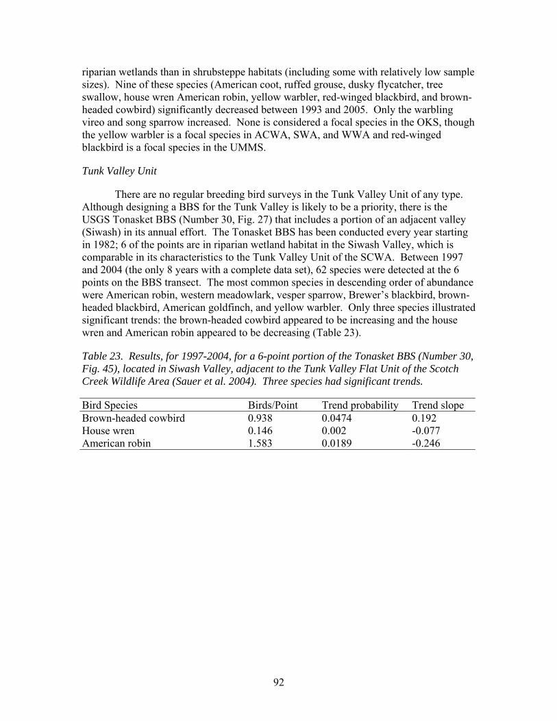
92
riparian wetlands than in shrubsteppe habitats (including some with relatively low sample sizes). Nine of these species (American coot, ruffed grouse, dusky flycatcher, tree swallow, house wren American robin, yellow warbler, red-winged blackbird, and brown-headed cowbird) significantly decreased between 1993 and 2005. Only the warbling vireo and song sparrow increased. None is considered a focal species in the OKS, though the yellow warbler is a focal species in ACWA, SWA, and WWA and red-winged blackbird is a focal species in the UMMS.
Tunk Valley Unit
There are no regular breeding bird surveys in the Tunk Valley Unit of any type. Although designing a BBS for the Tunk Valley is likely to be a priority, there is the USGS Tonasket BBS (Number 30, Fig. 27) that includes a portion of an adjacent valley (Siwash) in its annual effort. The Tonasket BBS has been conducted every year starting in 1982; 6 of the points are in riparian wetland habitat in the Siwash Valley, which is comparable in its characteristics to the Tunk Valley Unit of the SCWA. Between 1997 and 2004 (the only 8 years with a complete data set), 62 species were detected at the 6 points on the BBS transect. The most common species in descending order of abundance were American robin, western meadowlark, vesper sparrow, Brewer’s blackbird, brown-headed blackbird, American goldfinch, and yellow warbler. Only three species illustrated significant trends: the brown-headed cowbird appeared to be increasing and the house wren and American robin appeared to be decreasing (Table 23).
Table 23. Results, for 1997-2004, for a 6-point portion of the Tonasket BBS (Number 30, Fig. 45), located in Siwash Valley, adjacent to the Tunk Valley Flat Unit of the Scotch Creek Wildlife Area (Sauer et al. 2004). Three species had significant trends.
Bird Species Birds/Point Trend probability Trend slope Brown-headed cowbird 0.938 0.0474 0.192 House wren 0.146 0.002 -0.077 American robin 1.583 0.0189 -0.246
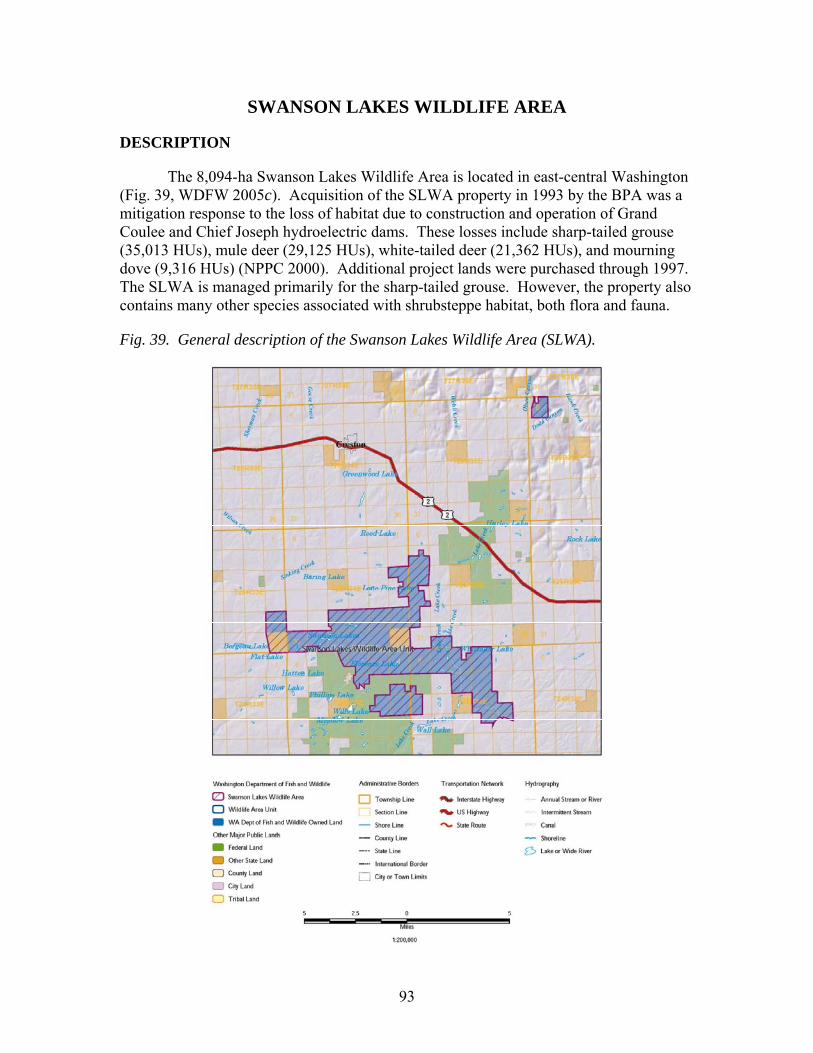
93
SWANSON LAKES WILDLIFE AREA
DESCRIPTION
The 8,094-ha Swanson Lakes Wildlife Area is located in east-central Washington (Fig. 39, WDFW 2005c). Acquisition of the SLWA property in 1993 by the BPA was a mitigation response to the loss of habitat due to construction and operation of Grand Coulee and Chief Joseph hydroelectric dams. These losses include sharp-tailed grouse (35,013 HUs), mule deer (29,125 HUs), white-tailed deer (21,362 HUs), and mourning dove (9,316 HUs) (NPPC 2000). Additional project lands were purchased through 1997. The SLWA is managed primarily for the sharp-tailed grouse. However, the property also contains many other species associated with shrubsteppe habitat, both flora and fauna.
Fig. 39. General description of the Swanson Lakes Wildlife Area (SLWA).
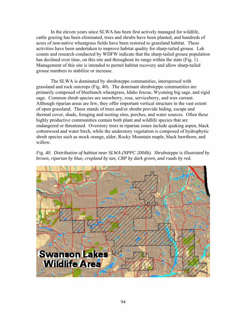
94
In the eleven years since SLWA has been first actively managed for wildlife, cattle grazing has been eliminated, trees and shrubs have been planted, and hundreds of acres of non-native wheatgrass fields have been restored to grassland habitat. These activities have been undertaken to improve habitat quality for sharp-tailed grouse. Lek counts and research conducted by WDFW indicate that the sharp-tailed grouse population has declined over time, on this site and throughout its range within the state (Fig. 1). Management of this site is intended to permit habitat recovery and allow sharp-tailed grouse numbers to stabilize or increase.
The SLWA is dominated by shrubsteppe communities, interspersed with grassland and rock outcrops (Fig. 40). The dominant shrubsteppe communities are primarily composed of bluebunch wheatgrass, Idaho fescue, Wyoming big sage, and rigid sage. Common shrub species are snowberry, rose, serviceberry, and wax currant. Although riparian areas are few, they offer important vertical structure in the vast extent of open grassland. These stands of trees and/or shrubs provide hiding, escape and thermal cover, shade, foraging and nesting sites, perches, and water sources. Often these highly productive communities contain both plant and wildlife species that are endangered or threatened. Overstory trees in riparian zones include quaking aspen, black cottonwood and water birch, while the understory vegetation is composed of hydrophytic shrub species such as mock orange, alder, Rocky Mountain maple, black hawthorn, and willow.
Fig. 40. Distribution of habitat near SLWA (NPPC 2004b). Shrubsteppe is illustrated by brown, riparian by blue, cropland by tan, CRP by dark green, and roads by red.
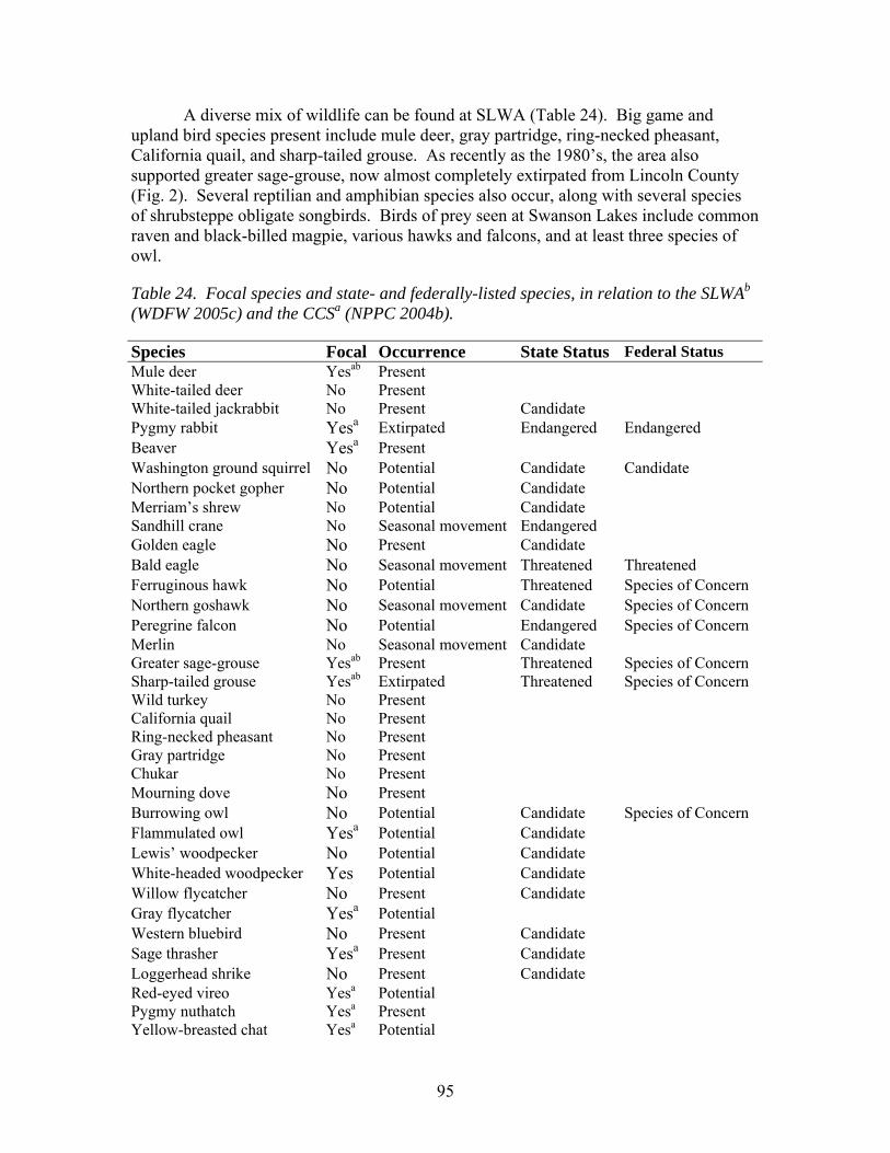
95
A diverse mix of wildlife can be found at SLWA (Table 24). Big game and upland bird species present include mule deer, gray partridge, ring-necked pheasant, California quail, and sharp-tailed grouse. As recently as the 1980’s, the area also supported greater sage-grouse, now almost completely extirpated from Lincoln County (Fig. 2). Several reptilian and amphibian species also occur, along with several species of shrubsteppe obligate songbirds. Birds of prey seen at Swanson Lakes include common raven and black-billed magpie, various hawks and falcons, and at least three species of owl.
Table 24. Focal species and state- and federally-listed species, in relation to the SLWAb (WDFW 2005c) and the CCSa (NPPC 2004b).
Species Focal Occurrence State Status Federal Status Mule deer Yesab Present White-tailed deer No Present White-tailed jackrabbit No Present Candidate Pygmy rabbit Yesa Extirpated Endangered Endangered Beaver Yesa Present Washington ground squirrel No Potential Candidate Candidate Northern pocket gopher No Potential Candidate Merriam’s shrew No Potential Candidate Sandhill crane No Seasonal movement Endangered Golden eagle No Present Candidate Bald eagle No Seasonal movement Threatened Threatened Ferruginous hawk No Potential Threatened Species of Concern Northern goshawk No Seasonal movement Candidate Species of Concern Peregrine falcon No Potential Endangered Species of Concern Merlin No Seasonal movement Candidate Greater sage-grouse Yesab Present Threatened Species of Concern Sharp-tailed grouse Yesab Extirpated Threatened Species of Concern Wild turkey No Present California quail No Present Ring-necked pheasant No Present Gray partridge No Present Chukar No Present Mourning dove No Present Burrowing owl No Potential Candidate Species of Concern Flammulated owl Yesa Potential Candidate Lewis’ woodpecker No Potential Candidate White-headed woodpecker Yes Potential Candidate Willow flycatcher No Present Candidate Gray flycatcher Yesa Potential Western bluebird No Present Candidate Sage thrasher Yesa Present Candidate Loggerhead shrike No Present Candidate Red-eyed vireo Yesa Potential Pygmy nuthatch Yesa Present Yellow-breasted chat Yesa Potential
96
Grasshopper sparrow No Present Brewer’s sparrow No Present Sage sparrow No Present Candidate Vesper sparrow No Present Candidate Sagebrush lizard No Potential Candidate
Management goals for the SLWA are to preserve habitat and species diversity for wildlife resources, maintain healthy populations of game and non-game species, protect and restore native plant communities, and provide diverse opportunities for the public to encounter, utilize, and appreciate wildlife and wild areas (WDFW 2005c). Although the SLWA is primarily managed to promote recovery of the sharp-tailed grouse, management is also directed toward the protection and management of other shrubsteppe obligate species (WDFW 2005c). Some of these specific objectives are listed below:
1. Manage for upland birds including sharp-tailed grouse, gray partridge, California quail, and ring-necked pheasant. Strategies include: 1) Conduct annual lek surveys for sharp-tailed grouse; 2) Restore native-like grasslands; 3) Maintain upland feeders, food plots, and guzzlers; 4) Genetically augmentation of the sharp-tailed grouse population; and 5) Remove man-made nesting structures used by common ravens.
2. Manage and protect diverse assemblages of species. Strategies include: 1) Management of Spalding’s catchfly to ensure that weed control activities, and other activities on the ground, do not damage existing colonies; 2) Continue to support BLM and WSU in their study of badger movements; 3) Continue to work with WDNR to map and manage species of concern; 4) Assist WDFW and other agency staff in finding and assessing sites at SLWA for possible pygmy rabbit introductions; 5) Continue to support WDFW’s comprehensive shrubsteppe study; 6) Protect and maintain waterfowl and shorebird habitats; and 7) Assist in non-game activities and surveys.
3. Manage populations of big game, particularly mule deer. Many of the same strategies applied to sharp-tailed grouse will also benefit mule deer. In addition, controlled burns and guzzlers will be considered.
4. Improve and maintain fish populations, although no native fish populations are known to exist in the upper reaches of Lake Creek, which runs through SLWA. Strategies include restoration of riparian habitat and associated fences along Lake Creek.
5. Protect and restore riparian habitat by planting trees and shrubs and/or fencing where necessary.
6. Protect and restore shrubsteppe habitat by: 1) Assessing habitat quality and mapping; 2) Applying integrated pest management to areas with noxious weeds; and 3) Consideration of local plant biotypes in future plantings.
97
CRAB CREEK SUBBASIN
The NPPC (2004b) recommends specific strategies to address habitat and biological objectives in three focal habitats; shrubsteppe, riparian wetland, and Ponderosa pine. While all habitats are important, these focal habitats were selected in part because they are disproportionately vulnerable to anthropogenic impacts, and likely have received the highest level of impacts within the subbasin. Some of the identified impacts are, for all practical purposes, irreversible and others are already being mitigated through ongoing management. Many focal species (Table 24) are considered within these focal habitats including: 1) white-headed woodpecker, pygmy nuthatch, gray flycatcher, and flammulated owl in Ponderosa pine; 2) sharp-tailed grouse, greater sage-grouse, mule deer, sage thrasher, and pygmy rabbit in shrubsteppe; and 3) red-eyed vireo, yellow-breasted chat, and American beaver in riparian wetlands.
The NPPC (2004b) recommends the development of an integrated monitoring program that influences adaptive management. The NPPC also recommends selection of a survey protocol to measure the abundance of focal species (Table 23) and to measure diversity and richness of species assemblages within each habitat type. In certain cases, this could include the evaluation of population status for each focal species in each focal habitat type. In addition, the NPPC (2004b) recommends inventory of other shrubsteppe, riparian wetland, and Ponderosa pine obligates in an effort to test assumptions of the umbrella species concept.
MONITORING AND EVALUATION
Habitat
HEP transects have been conducted on the SLWA between 1990 and 2006 (Table 25). Much of the habitat data was collected to address specific management questions, rather than providing the baseline data for long-term monitoring. A preliminary assessment of habitat shows that there were trends in the data (Table 25). VOR, grass cover, and forb cover appeared to increase in shrubsteppe habitats. Grass cover tended to increase and VOR tended to decrease in CRP habitats. Riparian habitats had data that was too limited for long-term analysis (Table 25). It is not certain at this stage if all the data that has been collected is currently available (see transect map for the SLWA (Fig. 41). Data management for the SLWA and all other wildlife areas will be an ongoing process.
Table 25. Preliminary summary of data from HEP transects on the SLWA.
Shrubsteppe CRP Riparian Habitat parameter 1990-1996 2000-2006 1990-1996 2000-2006 1995 Number of transects 35 39 14 3 6 VOR (cm) 4.2 5.1 7.4 6.0 Tree cover (%) 13.3 Shrub cover (%) 10.8 9.7 0.1 0.4 41.9 Shrub height (m) 0.5 0.5 0.2
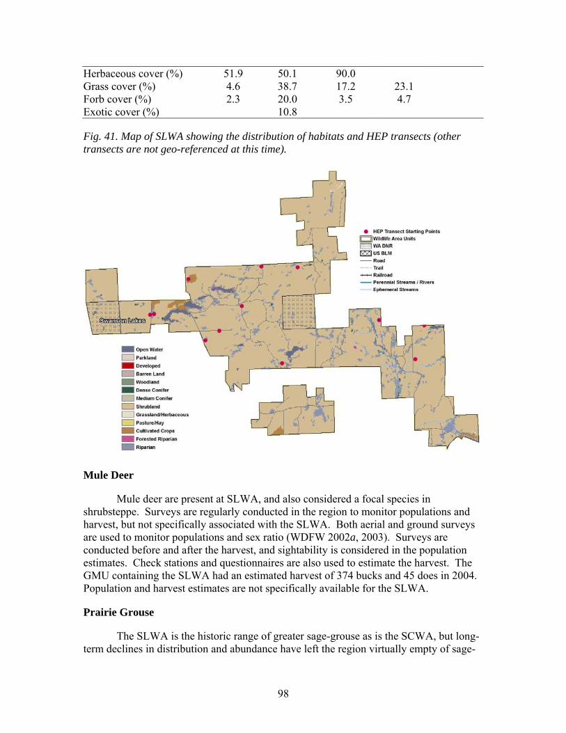
98
Herbaceous cover (%) 51.9 50.1 90.0 Grass cover (%) 4.6 38.7 17.2 23.1 Forb cover (%) 2.3 20.0 3.5 4.7 Exotic cover (%) 10.8
Fig. 41. Map of SLWA showing the distribution of habitats and HEP transects (other transects are not geo-referenced at this time).
Mule Deer
Mule deer are present at SLWA, and also considered a focal species in shrubsteppe. Surveys are regularly conducted in the region to monitor populations and harvest, but not specifically associated with the SLWA. Both aerial and ground surveys are used to monitor populations and sex ratio (WDFW 2002a, 2003). Surveys are conducted before and after the harvest, and sightability is considered in the population estimates. Check stations and questionnaires are also used to estimate the harvest. The GMU containing the SLWA had an estimated harvest of 374 bucks and 45 does in 2004. Population and harvest estimates are not specifically available for the SLWA.
Prairie Grouse
The SLWA is the historic range of greater sage-grouse as is the SCWA, but long-term declines in distribution and abundance have left the region virtually empty of sage-

99
grouse (Fig. 42). The last confirmed active lek disappeared after 1986 adjacent to the SLWA. Sage-grouse are occasionally observed in the area, suggesting that there may be potential for range expansion or habitat support for a translocated group of birds. An effort to re-establish sage-grouse in the area was initiated in 2008.
Fig. 42. Estimated greater sage-grouse population, based on lek surveys, between 1957 and 2005, in the CCS and in the immediate vicinity of the SLWA.
0
100
200
300
400
500
600
1955 1960 1965 1970 1975 1980 1985 1990 1995 2000 2005
Year
Popu
latio
n es
timat
e
Crab Creek Subbasin
Swanson Lakes Wildlife Area
Similar to sage-grouse, sharp-tailed grouse have dramatically declined in the region near the SLWA during the last 35 years and populations are limited to relatively small and isolated pockets of birds. The CCS and SLWA populations show similar tendencies to the rangewide population (Fig. 43). The 2005 population in the region was estimated to be approximately 42 in the CCS and 28 in the SLWA.
Fig. 43. Estimated sharp-tailed grouse population, based on lek surveys, between 1964 and 2008, in the CCS and in the immediate vicinity of the SLWA.
0
50
100
150
200
250
300
350
400
450
1964 1968 1972 1976 1980 1984 1988 1992 1996 2000 2004 2008
Popu
latio
n es
timat
e
100
Because the low number of birds on SLWA (estimated to be 62 in 2008) is not believed to be viable, an augmentation program for sharp-tailed grouse was initiated in 2005. Sharp-tailed grouse have been captured in the wild in southern British Columbia, southeastern Idaho, and northern Utah and translocated to Washington in each year through at least 2009. It is hoped that these birds will interbred with the resident birds and strength the population both genetically and demographically.
General Bird Surveys
Annual breeding bird surveys were conducted on and near the SLWA between 1994 and 2005 (surveys conducted every year except 2004). Surveys were designed to sample ‘control’ (off the wildlife areas) and ‘treatment’ (on the wildlife area) sites. In addition, survey points were selected to reflect the two focal habitats, shrubsteppe and riparian wetland, as well as small lakes on and off the SLWA. The analysis was conducted with a general linear model using the number of birds as the dependent variable, and treatment (on or off the study area), habitat (shrubsteppe or riparian wetland), and year (continuous variable between 1994 and 2005) as independent variables. Although the lakes were not considered in the statistical analysis, different species of birds that were detected at the lakes were included in the results.
During these surveys, muskrat, coyote, mule deer, yellow pine chipmunk, yellow-bellied marmot, and Washington ground squirrel were mammals that were detected. Many bird species were detected (101), 66 of which were detected infrequently (< 0.05 detections/point). Eighteen species had significantly different abundance on shrubsteppe and riparian wetland sites (Table 26); five of these species also had significant annual variation (1 increasing and 4 decreasing). Three species significantly varied between control and treatment locations (Table 27); one significantly declined between 1994 and 2005. Ten species significantly varied by treatment and habitat type (Table 28); three of these also had annual variation (2 increasing and 1 decreasing). The red-tailed hawk (P = 0.0312) and morning dove (P = 0.0001) both declined significantly during the course of this study, but showed no significant differences by treatment or habitat type.
Two of the three focal bird species for shrubsteppe in the CCS were detected on the SLWA; sharp-tailed grouse and sage thrasher were detected and the greater sage-grouse was not detected. The sharp-tailed grouse was not observed enough to provide much data for analysis. Data for the sage thrasher indicated that they were significantly more common in shrubsteppe than in riparian wetland and more common on SLWA than off SLWA. The red-eyed vireo and yellow-breasted chat were the only two riparian wetland focal bird species in the CCS and neither was detected on the SLWA. There is not much potential habitat for either of these species on the SLWA. There are other focal species considered on BPA-funded wildlife areas that were also considered here. The great blue heron was only observed in shallow lakes and not in the previously defined riparian wetland. The Lewis’ woodpecker was not observed. Mallard, willow flycatcher, yellow warbler, and red-winged blackbird were all observed in greater abundance in riparian wetland than in shrubsteppe (Table 26, Table 28). The sage sparrow was not observed, but the grasshopper sparrow and Brewer’s sparrow were more common in shrubsteppe than riparian wetland.
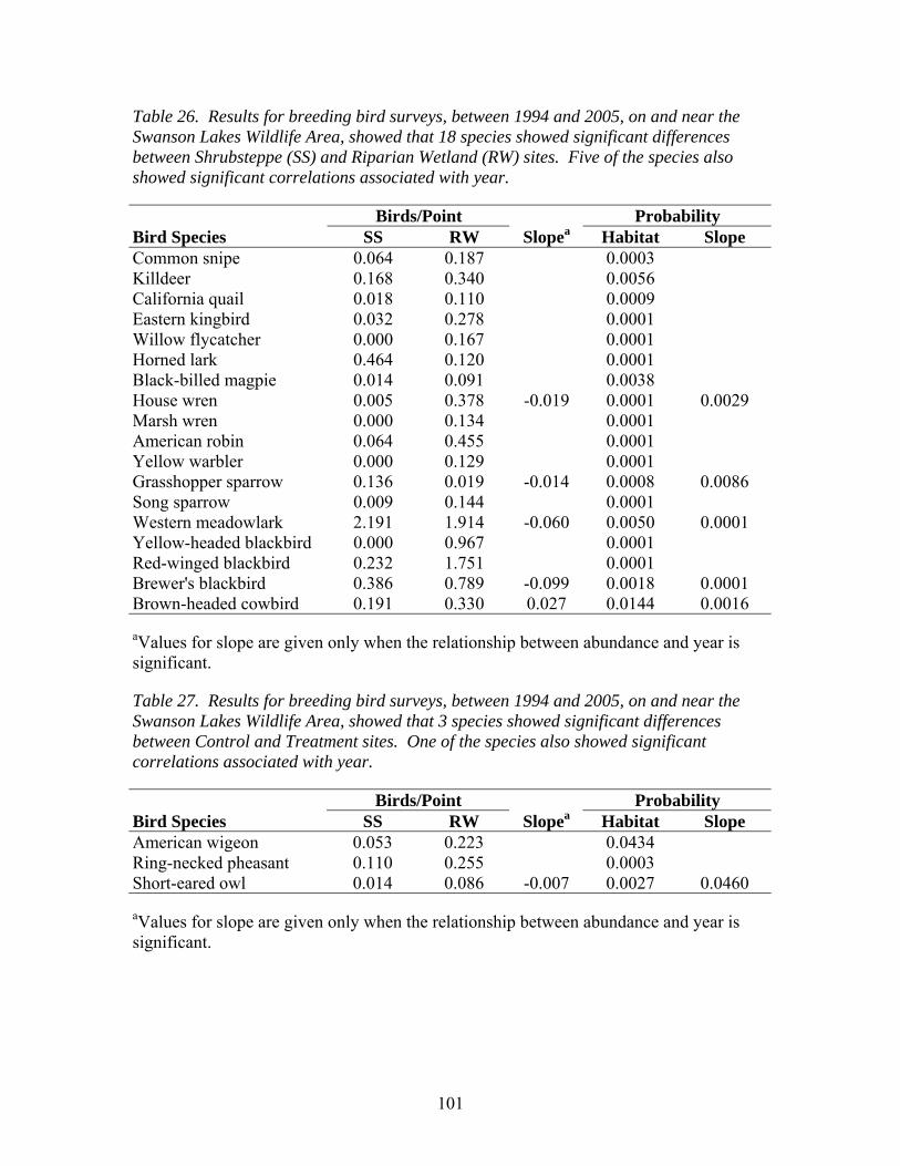
101
Table 26. Results for breeding bird surveys, between 1994 and 2005, on and near the Swanson Lakes Wildlife Area, showed that 18 species showed significant differences between Shrubsteppe (SS) and Riparian Wetland (RW) sites. Five of the species also showed significant correlations associated with year.
Birds/Point Probability Bird Species SS RW Slopea Habitat Slope Common snipe 0.064 0.187 0.0003 Killdeer 0.168 0.340 0.0056 California quail 0.018 0.110 0.0009 Eastern kingbird 0.032 0.278 0.0001 Willow flycatcher 0.000 0.167 0.0001 Horned lark 0.464 0.120 0.0001 Black-billed magpie 0.014 0.091 0.0038 House wren 0.005 0.378 -0.019 0.0001 0.0029 Marsh wren 0.000 0.134 0.0001 American robin 0.064 0.455 0.0001 Yellow warbler 0.000 0.129 0.0001 Grasshopper sparrow 0.136 0.019 -0.014 0.0008 0.0086 Song sparrow 0.009 0.144 0.0001 Western meadowlark 2.191 1.914 -0.060 0.0050 0.0001 Yellow-headed blackbird 0.000 0.967 0.0001 Red-winged blackbird 0.232 1.751 0.0001 Brewer's blackbird 0.386 0.789 -0.099 0.0018 0.0001 Brown-headed cowbird 0.191 0.330 0.027 0.0144 0.0016
aValues for slope are given only when the relationship between abundance and year is significant.
Table 27. Results for breeding bird surveys, between 1994 and 2005, on and near the Swanson Lakes Wildlife Area, showed that 3 species showed significant differences between Control and Treatment sites. One of the species also showed significant correlations associated with year.
Birds/Point Probability Bird Species SS RW Slopea Habitat Slope American wigeon 0.053 0.223 0.0434 Ring-necked pheasant 0.110 0.255 0.0003 Short-eared owl 0.014 0.086 -0.007 0.0027 0.0460
aValues for slope are given only when the relationship between abundance and year is significant.
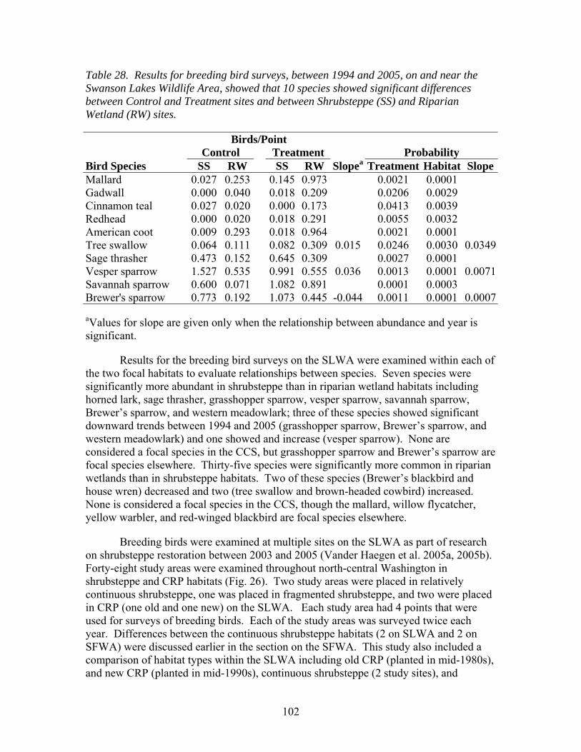
102
Table 28. Results for breeding bird surveys, between 1994 and 2005, on and near the Swanson Lakes Wildlife Area, showed that 10 species showed significant differences between Control and Treatment sites and between Shrubsteppe (SS) and Riparian Wetland (RW) sites.
Birds/Point Control Treatment Probability Bird Species SS RW SS RW Slopea Treatment Habitat SlopeMallard 0.027 0.253 0.145 0.973 0.0021 0.0001 Gadwall 0.000 0.040 0.018 0.209 0.0206 0.0029 Cinnamon teal 0.027 0.020 0.000 0.173 0.0413 0.0039 Redhead 0.000 0.020 0.018 0.291 0.0055 0.0032 American coot 0.009 0.293 0.018 0.964 0.0021 0.0001 Tree swallow 0.064 0.111 0.082 0.309 0.015 0.0246 0.0030 0.0349Sage thrasher 0.473 0.152 0.645 0.309 0.0027 0.0001 Vesper sparrow 1.527 0.535 0.991 0.555 0.036 0.0013 0.0001 0.0071Savannah sparrow 0.600 0.071 1.082 0.891 0.0001 0.0003 Brewer's sparrow 0.773 0.192 1.073 0.445 -0.044 0.0011 0.0001 0.0007
aValues for slope are given only when the relationship between abundance and year is significant.
Results for the breeding bird surveys on the SLWA were examined within each of the two focal habitats to evaluate relationships between species. Seven species were significantly more abundant in shrubsteppe than in riparian wetland habitats including horned lark, sage thrasher, grasshopper sparrow, vesper sparrow, savannah sparrow, Brewer’s sparrow, and western meadowlark; three of these species showed significant downward trends between 1994 and 2005 (grasshopper sparrow, Brewer’s sparrow, and western meadowlark) and one showed and increase (vesper sparrow). None are considered a focal species in the CCS, but grasshopper sparrow and Brewer’s sparrow are focal species elsewhere. Thirty-five species were significantly more common in riparian wetlands than in shrubsteppe habitats. Two of these species (Brewer’s blackbird and house wren) decreased and two (tree swallow and brown-headed cowbird) increased. None is considered a focal species in the CCS, though the mallard, willow flycatcher, yellow warbler, and red-winged blackbird are focal species elsewhere.
Breeding birds were examined at multiple sites on the SLWA as part of research on shrubsteppe restoration between 2003 and 2005 (Vander Haegen et al. 2005a, 2005b). Forty-eight study areas were examined throughout north-central Washington in shrubsteppe and CRP habitats (Fig. 26). Two study areas were placed in relatively continuous shrubsteppe, one was placed in fragmented shrubsteppe, and two were placed in CRP (one old and one new) on the SLWA. Each study area had 4 points that were used for surveys of breeding birds. Each of the study areas was surveyed twice each year. Differences between the continuous shrubsteppe habitats (2 on SLWA and 2 on SFWA) were discussed earlier in the section on the SFWA. This study also included a comparison of habitat types within the SLWA including old CRP (planted in mid-1980s), and new CRP (planted in mid-1990s), continuous shrubsteppe (2 study sites), and
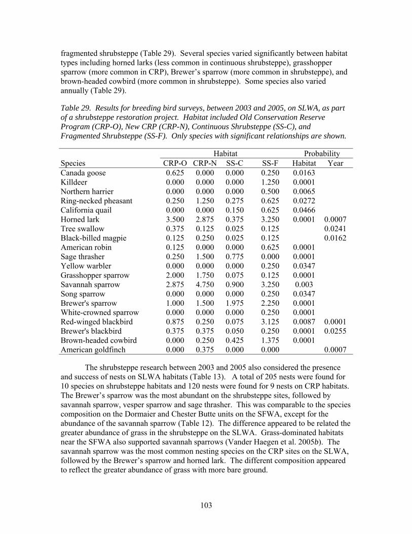
103
fragmented shrubsteppe (Table 29). Several species varied significantly between habitat types including horned larks (less common in continuous shrubsteppe), grasshopper sparrow (more common in CRP), Brewer’s sparrow (more common in shrubsteppe), and brown-headed cowbird (more common in shrubsteppe). Some species also varied annually (Table 29).
Table 29. Results for breeding bird surveys, between 2003 and 2005, on SLWA, as part of a shrubsteppe restoration project. Habitat included Old Conservation Reserve Program (CRP-O), New CRP (CRP-N), Continuous Shrubsteppe (SS-C), and Fragmented Shrubsteppe (SS-F). Only species with significant relationships are shown.
Habitat Probability Species CRP-O CRP-N SS-C SS-F Habitat Year Canada goose 0.625 0.000 0.000 0.250 0.0163 Killdeer 0.000 0.000 0.000 1.250 0.0001 Northern harrier 0.000 0.000 0.000 0.500 0.0065 Ring-necked pheasant 0.250 1.250 0.275 0.625 0.0272 California quail 0.000 0.000 0.150 0.625 0.0466 Horned lark 3.500 2.875 0.375 3.250 0.0001 0.0007 Tree swallow 0.375 0.125 0.025 0.125 0.0241 Black-billed magpie 0.125 0.250 0.025 0.125 0.0162 American robin 0.125 0.000 0.000 0.625 0.0001 Sage thrasher 0.250 1.500 0.775 0.000 0.0001 Yellow warbler 0.000 0.000 0.000 0.250 0.0347 Grasshopper sparrow 2.000 1.750 0.075 0.125 0.0001 Savannah sparrow 2.875 4.750 0.900 3.250 0.003 Song sparrow 0.000 0.000 0.000 0.250 0.0347 Brewer's sparrow 1.000 1.500 1.975 2.250 0.0001 White-crowned sparrow 0.000 0.000 0.000 0.250 0.0001 Red-winged blackbird 0.875 0.250 0.075 3.125 0.0087 0.0001 Brewer's blackbird 0.375 0.375 0.050 0.250 0.0001 0.0255 Brown-headed cowbird 0.000 0.250 0.425 1.375 0.0001 American goldfinch 0.000 0.375 0.000 0.000 0.0007
The shrubsteppe research between 2003 and 2005 also considered the presence and success of nests on SLWA habitats (Table 13). A total of 205 nests were found for 10 species on shrubsteppe habitats and 120 nests were found for 9 nests on CRP habitats. The Brewer’s sparrow was the most abundant on the shrubsteppe sites, followed by savannah sparrow, vesper sparrow and sage thrasher. This was comparable to the species composition on the Dormaier and Chester Butte units on the SFWA, except for the abundance of the savannah sparrow (Table 12). The difference appeared to be related the greater abundance of grass in the shrubsteppe on the SLWA. Grass-dominated habitats near the SFWA also supported savannah sparrows (Vander Haegen et al. 2005b). The savannah sparrow was the most common nesting species on the CRP sites on the SLWA, followed by the Brewer’s sparrow and horned lark. The different composition appeared to reflect the greater abundance of grass with more bare ground.
104
Miscellaneous Surveys
Surveys for reptiles and amphibians were conducted on five different sites on the SLWA. The largest number and greatest diversity was found in continuous shrubsteppe habitat rather than in fragmented shrubsteppe or CRP. Some of the reptiles found include racer, western rattlesnake, gopher snake, western terrestrial garter snake, night snake, western skink, short-horned lizard. In addition, the great-basin spadefoot toad, long-toed salamander, and tiger salamander were found. The most common species found was the short-horned lizard. Surveys for mammals were conducted on, and near, the SLWA. Eleven species were captured (some on SFWA), but the most common was the deer mouse, followed by Great Basin pocket mouse, sagebrush vole, western harvest mouse, least chipmunk, and vagrant shrew (Table 14). Because of the preliminary nature of the data (Vander Haegen et al. 2005b), it is not possible to compare habitat types. However, it is likely that when the data is fully analyzed, it will provide useful insight into the structures of habitats as well as the configuration of landscapes.
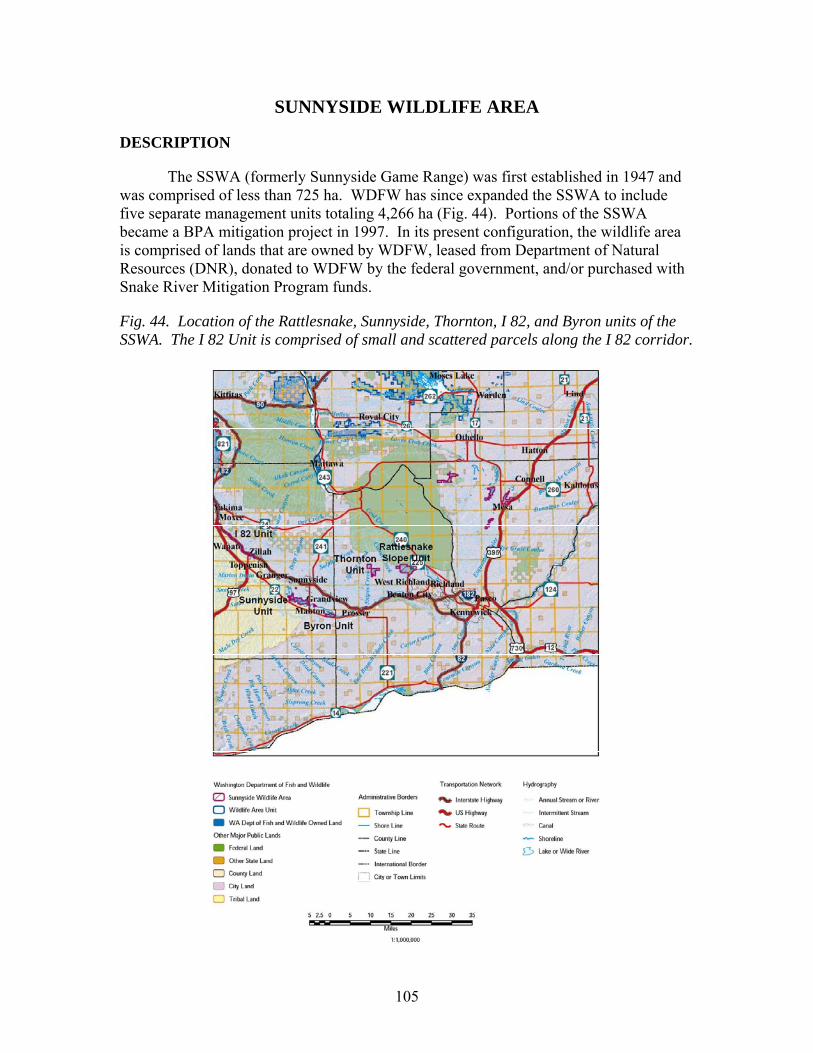
105
SUNNYSIDE WILDLIFE AREA
DESCRIPTION
The SSWA (formerly Sunnyside Game Range) was first established in 1947 and was comprised of less than 725 ha. WDFW has since expanded the SSWA to include five separate management units totaling 4,266 ha (Fig. 44). Portions of the SSWA became a BPA mitigation project in 1997. In its present configuration, the wildlife area is comprised of lands that are owned by WDFW, leased from Department of Natural Resources (DNR), donated to WDFW by the federal government, and/or purchased with Snake River Mitigation Program funds.
Fig. 44. Location of the Rattlesnake, Sunnyside, Thornton, I 82, and Byron units of the SSWA. The I 82 Unit is comprised of small and scattered parcels along the I 82 corridor.
106
The SSWA consists of the 1,128-ha Sunnyside Unit, the 397-ha I-82 Unit(s), 417-ha Byron Unit, the 1,482-ha Rattlesnake Slope Unit, and the 842-ha Thornton Unit. The SSWA has been approved as a wildlife mitigation project by BPA. This project will partially meet BPA's mitigation obligation to compensate for wildlife losses resulting from the construction of Grand Coulee, McNary and John Day Dams (Table 1). By funding the enhancement and reasonable operation and maintenance of the SSWA for the life of the project, BPA will receive credit towards its mitigation debt. Mallard, western meadowlark, Canada goose, yellow warbler, downy woodpecker, mink, California quail, black-capped chickadee, great blue heron, mule deer and greater sage-grouse were identified in the loss assessments and were used as HEP indicator species (Howerton 1986, BPA 1989, WDFW 1998).
Specific objectives include (WDFW 1998): 1) Provide optimum habitat for threatened and endangered species, priority species, waterfowl, upland birds, and shrubsteppe obligates; 2) Maximize public recreational opportunities; 3) Control the proliferation and spread of noxious weeds on upland, riparian, and wetland habitats; 4) Protect, maintain, and enhance shrubsteppe and riparian wetlands; 5) Maintain alfalfa fields and food plots to reduce waterfowl depredation on adjoining private croplands; 6) Provide and promote public recreational opportunities and enforcement of wildlife and environmental laws; 7) Improve water quality in wetlands and water flowing into the Yakima River; 8) Coordinate land management activities with the YIN, irrigation districts, NRCS, USFWS, Ducks Unlimited, and other interested stakeholders; and 9) Monitor wildlife populations in conjunction with monitoring and evaluation needs and established protocols.
YAKIMA SUBBASIN
The NPPC (2004f) recommends specific strategies to address habitat and biological objectives in four focal habitats; montane coniferous wetlands, Ponderosa Pine/Oregon white oak, shrubsteppe/interior grasslands, and interior riparian wetlands. Although shrubsteppe was lumped with grasslands in the subbasin plan, the habitat is considered shrubsteppe here because the SSWA is relatively low elevation and mostly in shrubsteppe. While all habitats are important, these focal habitats were selected in part because they are disproportionately vulnerable to anthropogenic impacts, and likely have received the highest level of impacts within the subbasin, and in adjacent subbasins. Some of the identified impacts are, for all practical purposes, irreversible and others are already being mitigated through ongoing management. Although many focal species are considered within these habitats (Table 30), only those on SSWA are considered here including: 1) Mule deer, Brewer’s sparrow, and greater sage-grouse in shrubsteppe; and 2) Yellow warbler, American beaver, and mallard in interior riparian wetlands.
Table 30. List of focal species and state- and federally-listed species, in relation to the SSWAb (WDFW 1998) and the YSa (NPPC 2004h).
Species Focal Occurrence State Status Federal Status Elk No Present Mule deer Yesab Present
107
Mink Yesb Potential Beaver Yesa Present Western gray squirrel Yesa Absent Threatened Species of Concern Great blue heron Yesb Present Sandhill crane Yesa Potential Endangered Canada goose No Present Mallard Yesab Present Golden eagle No Potential Candidate Bald eagle No Present Threatened Threatened Ferruginous hawk No Potential Threatened Species of Concern Northern goshawk No Potential Candidate Species of Concern Peregrine falcon No Potential Endangered Species of Concern Merlin No Potential Candidate Greater sage-grouse Yesab Extirpated Threatened Candidate California quail Yesb Present Burrowing owl No Potential Candidate Species of Concern Lewis’ woodpecker Yesa Potential Candidate White-headed woodpecker Yesa Potential Candidate Downy woodpecker Yesb Present Willow flycatcher No Potential Candidate Sage thrasher No Present Candidate Loggerhead shrike No Present Candidate Black-capped chickadee Yesb Present Yellow warbler Yesab Present Grasshopper sparrow Yesa Present Brewer’s sparrow Yesa Present Sage sparrow No Potential Candidate Vesper sparrow No Present Candidate Western meadowlark Yesb Present Western toad Yesa Potential Candidate Species of Concern
The NPPC (2004f) recommends the development of an integrated monitoring program that influences adaptive management. The NPPC also recommends selection of a survey protocol to measure the abundance of focal species (Table 30) and to measure diversity and richness of species assemblages within each habitat type. In certain cases, this could include the evaluation of population status for each focal species in each focal habitat type. In addition, the NPPC (2004f) recommends inventory of other shrubsteppe/grassland and riparian wetland obligates in an effort to test assumptions of the umbrella species concept.
MONITORING AND EVALUATION
Elk
The Yakima elk herd encompasses portions of the SSWA, but it is not a focal species. Nevertheless the herd is monitored annually, and its management is a fundamental issue on the wildlife area. The Yakima elk herd is divided into two sub-herds, the Cascade Slope sub-herd and the Rattlesnake Hills sub-herd (WDFW 2002b).
108
The Rattlesnake Hills sub-herd spends most of the year in the Rattlesnake Hills (managed mostly by DOE), but can be found over a broad area, particularly in winter. Because it is primarily found in the Rattlesnake Hills, elk regularly use the Rattlesnake Slope Unit of the SSWA. The estimates for this sub-herd averaged 686 between 1999 and 2001, which is substantially higher than the target number (about 375). In addition, the WDFW has a goal for a bull:cow ratio of 15:100 to 35:100 before the hunting season and 12:100 to 20:100 after the hunting season (WDFW 2002a). Consequently efforts are underway to reduce the sub-herd. The 2004 harvest in the GMU was estimated to be 13 bulls and 33 cows. Elk from this sub-herd also were translocated to ACWA in 2000. Aerial surveys are conducted in summer following the calving season and in winter following the hunting season. DOE plans to continue conducting annual surveys of the Yakima elk herd.
Mule Deer
Mule deer are present on the SSWA, and are considered a focal species in shrubsteppe. Surveys are regularly conducted in the region, not specifically associated with the SSWA, to monitor populations and harvest. Both aerial and ground surveys are used to monitor populations and sex ratio (WDFW 2002a, 2003). Surveys are conducted before and after the harvest, and sightability is considered in the population estimates. Check stations and questionnaires are also used to estimate the harvest. The GMU containing the SSWA had an estimated harvest of 93 bucks and 1 doe in 2004. Population and harvest estimates are not specifically available for the SSWA.
Miscellaneous Surveys
Waterfowl surveys are regularly conducted in, and around, the SSWA. This data is currently unavailable. The SSWA is the historic range of greater sage-grouse and sharp-tailed grouse, but long-term declines in distribution and abundance have left the region essentially empty of prairie grouse. Lek surveys are done annually in all areas with known populations. Unfortunately, there are no USGS BBSs near the SSWA (Fig. 27). Consequently, establishment of breeding bird surveys is an important first step for obtaining baseline information on priority species.
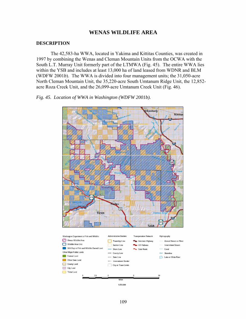
109
WENAS WILDLIFE AREA
DESCRIPTION
The 42,583-ha WWA, located in Yakima and Kittitas Counties, was created in 1997 by combining the Wenas and Cleman Mountain Units from the OCWA with the South L.T. Murray Unit formerly part of the LTMWA (Fig. 45). The entire WWA lies within the YSB and includes at least 13,000 ha of land leased from WDNR and BLM (WDFW 2001b). The WWA is divided into four management units; the 31,050-acre North Cleman Mountain Unit, the 35,220-acre South Umtanum Ridge Unit, the 12,852-acre Roza Creek Unit, and the 26,099-acre Umtanum Creek Unit (Fig. 46).
Fig. 45. Location of WWA in Washington (WDFW 2001b).
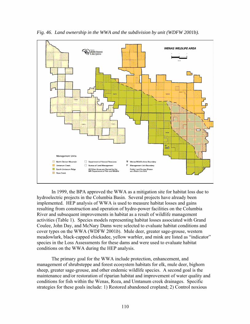
110
Fig. 46. Land ownership in the WWA and the subdivision by unit (WDFW 2001b).
In 1999, the BPA approved the WWA as a mitigation site for habitat loss due to hydroelectric projects in the Columbia Basin. Several projects have already been implemented. HEP analysis of WWA is used to measure habitat losses and gains resulting from construction and operation of hydro-power facilities on the Columbia River and subsequent improvements in habitat as a result of wildlife management activities (Table 1). Species models representing habitat losses associated with Grand Coulee, John Day, and McNary Dams were selected to evaluate habitat conditions and cover types on the WWA (WDFW 2001b). Mule deer, greater sage-grouse, western meadowlark, black-capped chickadee, yellow warbler, and mink are listed as “indicator” species in the Loss Assessments for these dams and were used to evaluate habitat conditions on the WWA during the HEP analysis.
The primary goal for the WWA include protection, enhancement, and management of shrubsteppe and forest ecosystem habitats for elk, mule deer, bighorn sheep, greater sage-grouse, and other endemic wildlife species. A second goal is the maintenance and/or restoration of riparian habitat and improvement of water quality and conditions for fish within the Wenas, Roza, and Umtanum creek drainages. Specific strategies for these goals include: 1) Restored abandoned cropland; 2) Control noxious
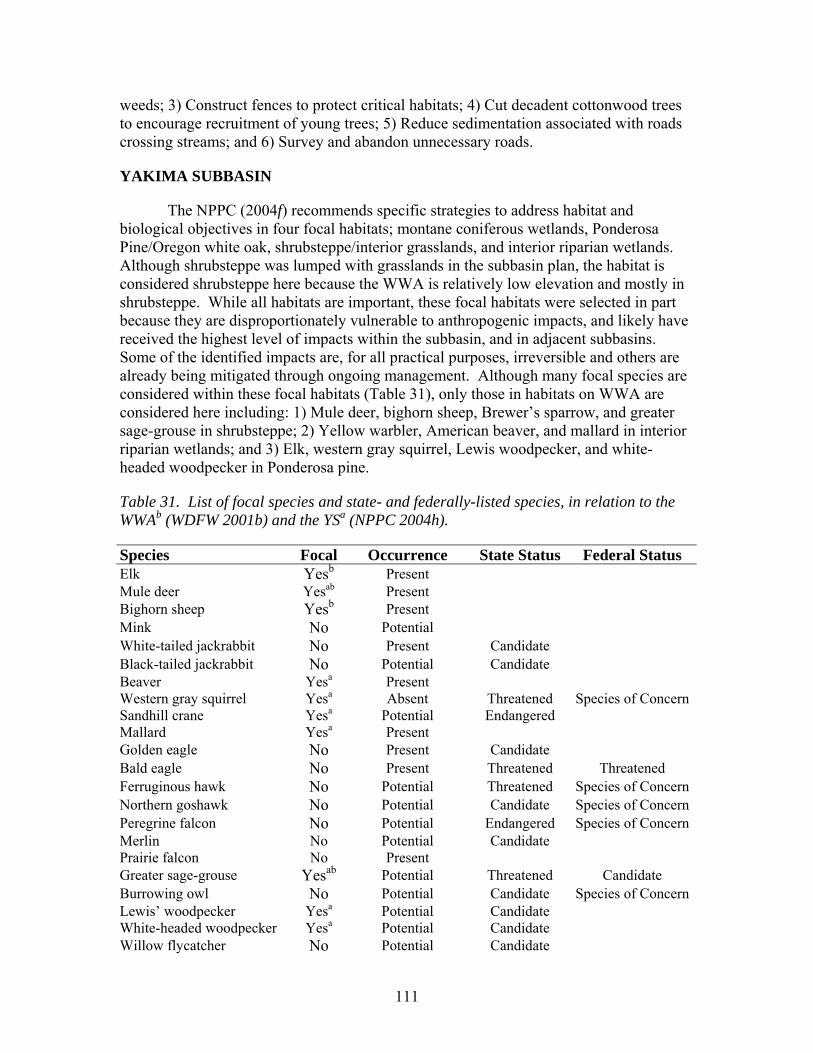
111
weeds; 3) Construct fences to protect critical habitats; 4) Cut decadent cottonwood trees to encourage recruitment of young trees; 5) Reduce sedimentation associated with roads crossing streams; and 6) Survey and abandon unnecessary roads.
YAKIMA SUBBASIN
The NPPC (2004f) recommends specific strategies to address habitat and biological objectives in four focal habitats; montane coniferous wetlands, Ponderosa Pine/Oregon white oak, shrubsteppe/interior grasslands, and interior riparian wetlands. Although shrubsteppe was lumped with grasslands in the subbasin plan, the habitat is considered shrubsteppe here because the WWA is relatively low elevation and mostly in shrubsteppe. While all habitats are important, these focal habitats were selected in part because they are disproportionately vulnerable to anthropogenic impacts, and likely have received the highest level of impacts within the subbasin, and in adjacent subbasins. Some of the identified impacts are, for all practical purposes, irreversible and others are already being mitigated through ongoing management. Although many focal species are considered within these focal habitats (Table 31), only those in habitats on WWA are considered here including: 1) Mule deer, bighorn sheep, Brewer’s sparrow, and greater sage-grouse in shrubsteppe; 2) Yellow warbler, American beaver, and mallard in interior riparian wetlands; and 3) Elk, western gray squirrel, Lewis woodpecker, and white-headed woodpecker in Ponderosa pine.
Table 31. List of focal species and state- and federally-listed species, in relation to the WWAb (WDFW 2001b) and the YSa (NPPC 2004h).
Species Focal Occurrence State Status Federal Status Elk Yesb Present Mule deer Yesab Present Bighorn sheep Yesb Present Mink No Potential White-tailed jackrabbit No Present Candidate Black-tailed jackrabbit No Potential Candidate Beaver Yesa Present Western gray squirrel Yesa Absent Threatened Species of Concern Sandhill crane Yesa Potential Endangered Mallard Yesa Present Golden eagle No Present Candidate Bald eagle No Present Threatened Threatened Ferruginous hawk No Potential Threatened Species of Concern Northern goshawk No Potential Candidate Species of Concern Peregrine falcon No Potential Endangered Species of Concern Merlin No Potential Candidate Prairie falcon No Present Greater sage-grouse Yesab Potential Threatened Candidate Burrowing owl No Potential Candidate Species of Concern Lewis’ woodpecker Yesa Potential Candidate White-headed woodpecker Yesa Potential Candidate Willow flycatcher No Potential Candidate
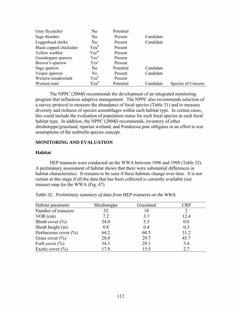
112
Gray flycatcher No Potential Sage thrasher No Present Candidate Loggerhead shrike No Present Candidate Black-capped chickadee Yesb Present Yellow warbler Yesab Present Grasshopper sparrow Yesa Present Brewer’s sparrow Yesa Present Sage sparrow No Potential Candidate Vesper sparrow No Present Candidate Western meadowlark Yesb Present Western toad Yesa Potential Candidate Species of Concern
The NPPC (2004f) recommends the development of an integrated monitoring program that influences adaptive management. The NPPC also recommends selection of a survey protocol to measure the abundance of focal species (Table 31) and to measure diversity and richness of species assemblages within each habitat type. In certain cases, this could include the evaluation of population status for each focal species in each focal habitat type. In addition, the NPPC (2004f) recommends, inventory of other shrubsteppe/grassland, riparian wetland, and Ponderosa pine obligates in an effort to test assumptions of the umbrella species concept.
MONITORING AND EVALUATION
Habitat
HEP transects were conducted on the WWA between 1996 and 1998 (Table 32). A preliminary assessment of habitat shows that there were substantial differences in habitat characteristics. It remains to be seen if these habitats change over time. It is not certain at this stage if all the data that has been collected is currently available (see transect map for the WWA (Fig. 47).
Table 32. Preliminary summary of data from HEP transects on the WWA.
Habitat parameter Shrubsteppe Grassland CRP Number of transects 32 18 2 VOR (cm) 7.2 3.7 12.4 Shrub cover (%) 24.0 5.5 0.6 Shrub height (m) 0.8 0.4 0.3 Herbaceous cover (%) 64.2 60.5 51.2 Grass cover (%) 28.8 29.7 45.7 Forb cover (%) 34.3 29.1 3.4 Exotic cover (%) 17.9 15.5 2.7

113
Fig. 47. Map of WWA showing the distribution of habitats and HEP transects.
Elk
The Yakima elk herd encompasses portions of the WWA, but it is not a focal species within the YS. Nevertheless the herd is monitored annually, and its management is a fundamental issue on the wildlife areas. The Yakima elk herd is divided into two sub-herds, the Cascade Slope sub-herd and the Rattlesnake Hills sub-herd (WDFW 2002b). The Cascade Slope sub-herd is found over a broad area, but regularly winters in portions of the WWA. The average population estimate for the potion in the GMU associated with the WWA was 5,191 elk between 1999 and 2001. The 2004 harvest in the GMU was estimated to be 57 bulls and 11 cows. The Rattlesnake Hills sub-herd spends most of the year in the Rattlesnake Hills, but can be found over a broad area, particularly in winter. Although it is primarily found in the Rattlesnake Hills, it can also be found on portions of the WWA. The estimates for this sub-herd averaged 686 between 1999 and 2001, which is substantially higher than the target number (about 375). Consequently efforts are underway to reduce the sub-herd. In addition, the WDFW has a goal for a bull:cow ratio of 15:100 to 35:100 before the hunting season and 12:100 to 20:100 after the hunting season (WDFW 2002a). Aerial surveys are conducted in summer for the Rattlesnake Hills sub-herd, in September before the hunting season in the Cascade Slope sub-herd, and in winter following the hunting season for both sub-herds. Surveys of the Cascade Slope sub-herd require about 10 hours of helicopter flight time in
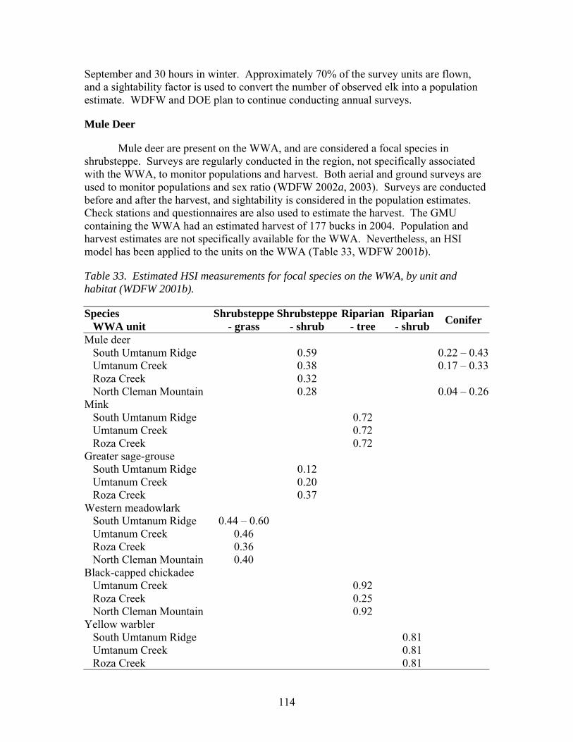
114
September and 30 hours in winter. Approximately 70% of the survey units are flown, and a sightability factor is used to convert the number of observed elk into a population estimate. WDFW and DOE plan to continue conducting annual surveys.
Mule Deer
Mule deer are present on the WWA, and are considered a focal species in shrubsteppe. Surveys are regularly conducted in the region, not specifically associated with the WWA, to monitor populations and harvest. Both aerial and ground surveys are used to monitor populations and sex ratio (WDFW 2002a, 2003). Surveys are conducted before and after the harvest, and sightability is considered in the population estimates. Check stations and questionnaires are also used to estimate the harvest. The GMU containing the WWA had an estimated harvest of 177 bucks in 2004. Population and harvest estimates are not specifically available for the WWA. Nevertheless, an HSI model has been applied to the units on the WWA (Table 33, WDFW 2001b).
Table 33. Estimated HSI measurements for focal species on the WWA, by unit and habitat (WDFW 2001b).
Species WWA unit
Shrubsteppe - grass
Shrubsteppe- shrub
Riparian - tree
Riparian - shrub Conifer
Mule deer South Umtanum Ridge 0.59 0.22 – 0.43 Umtanum Creek 0.38 0.17 – 0.33 Roza Creek 0.32 North Cleman Mountain 0.28 0.04 – 0.26Mink South Umtanum Ridge 0.72 Umtanum Creek 0.72 Roza Creek 0.72 Greater sage-grouse South Umtanum Ridge 0.12 Umtanum Creek 0.20 Roza Creek 0.37 Western meadowlark South Umtanum Ridge 0.44 – 0.60 Umtanum Creek 0.46 Roza Creek 0.36 North Cleman Mountain 0.40 Black-capped chickadee Umtanum Creek 0.92 Roza Creek 0.25 North Cleman Mountain 0.92 Yellow warbler South Umtanum Ridge 0.81 Umtanum Creek 0.81 Roza Creek 0.81
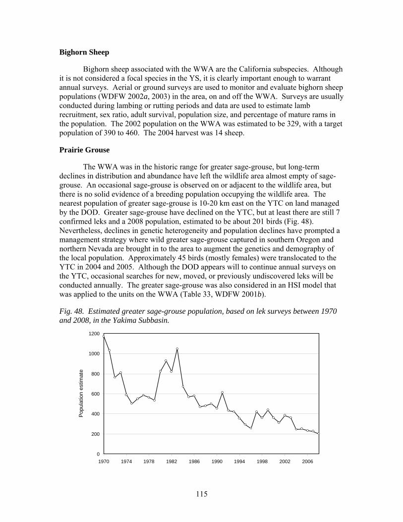
115
Bighorn Sheep
Bighorn sheep associated with the WWA are the California subspecies. Although it is not considered a focal species in the YS, it is clearly important enough to warrant annual surveys. Aerial or ground surveys are used to monitor and evaluate bighorn sheep populations (WDFW 2002a, 2003) in the area, on and off the WWA. Surveys are usually conducted during lambing or rutting periods and data are used to estimate lamb recruitment, sex ratio, adult survival, population size, and percentage of mature rams in the population. The 2002 population on the WWA was estimated to be 329, with a target population of 390 to 460. The 2004 harvest was 14 sheep.
Prairie Grouse
The WWA was in the historic range for greater sage-grouse, but long-term declines in distribution and abundance have left the wildlife area almost empty of sage-grouse. An occasional sage-grouse is observed on or adjacent to the wildlife area, but there is no solid evidence of a breeding population occupying the wildlife area. The nearest population of greater sage-grouse is 10-20 km east on the YTC on land managed by the DOD. Greater sage-grouse have declined on the YTC, but at least there are still 7 confirmed leks and a 2008 population, estimated to be about 201 birds (Fig. 48). Nevertheless, declines in genetic heterogeneity and population declines have prompted a management strategy where wild greater sage-grouse captured in southern Oregon and northern Nevada are brought in to the area to augment the genetics and demography of the local population. Approximately 45 birds (mostly females) were translocated to the YTC in 2004 and 2005. Although the DOD appears will to continue annual surveys on the YTC, occasional searches for new, moved, or previously undiscovered leks will be conducted annually. The greater sage-grouse was also considered in an HSI model that was applied to the units on the WWA (Table 33, WDFW 2001b).
Fig. 48. Estimated greater sage-grouse population, based on lek surveys between 1970 and 2008, in the Yakima Subbasin.
0
200
400
600
800
1000
1200
1970 1974 1978 1982 1986 1990 1994 1998 2002 2006
Popu
latio
n es
timat
e
116
General Bird Surveys
The USGS oversees the conducting of three BBSs (Fig. 27) in portions of the WWA (Selah, number 262; Ellensburg, number 44; and Yakima, number 81). Portions of the three transects traverse the WWA for about 114 of their combined 150 points. The points include the three focal habitats (shrubsteppe, riparian wetland, and Ponderosa pine) and two treatments (on and off the wildlife area). The points also cover portions of all the wildlife area units (only a small edge of the North Cleman Mountain Unit was covered). For purposes of this report, the data were combined for the four units. The BBS has been conducted every year since 2000 for Selah, 1993 for Yakima, and 1981 for Ellensburg.
A total of 116 species were observed on the combined BBS transects associated with the WWA; 44 of these had at least 0.05 observations/point while the others were too infrequent to consider in subsequent analysis. The most common of the 116 species detected in order of abundance were cliff swallow, western meadowlark, European starling, red-winged blackbird, American robin, Brewer’s blackbird, western wood-pewee, violet-green swallow, and Brewer’s sparrow.
Most of the focal species for the WWA including mallard, Lewis woodpecker, white-headed woodpecker, yellow warbler, and Brewer’s sparrow were detected during the BBSs. The only focal species not detected was the greater sage-grouse, primarily because it has largely been extirpated from the WWA. Focal species from other areas were also detected including the great blue heron, golden eagle, California quail, downy woodpecker, gray flycatcher, willow flycatcher, black-capped chickadee, pygmy nuthatch, sage thrasher, yellow-breasted chat, sage sparrow, western meadowlark, and red-winged blackbird.
Twenty-two species significantly varied by habitat type (Table 34). Most species were relatively common in riparian wetland, and to a lesser extent Ponderosa pine. Sage sparrow, Brewer’s sparrow, vesper sparrow were unusual in that they were most common in shrubsteppe. Two focal species for the WWA, the yellow warbler (riparian wetland) and Brewer’s sparrow (shrubsteppe), were more common in their focal habitats (Table 34), as expected. The yellow warbler also illustrated a significant increase between 1997 and 2004. An additional 6 species had abundance that varied significantly by treatment (on or off the WWA, Table 35). Eight additional species varied by both treatment and habitat (Table 36). The western meadowlark also illustrated a significant increase in abundance between 1997 and 2004. The western meadowlark and yellow warbler were also considered in an HSI model that was applied to the units on the WWA (Table 33, WDFW 2001b).
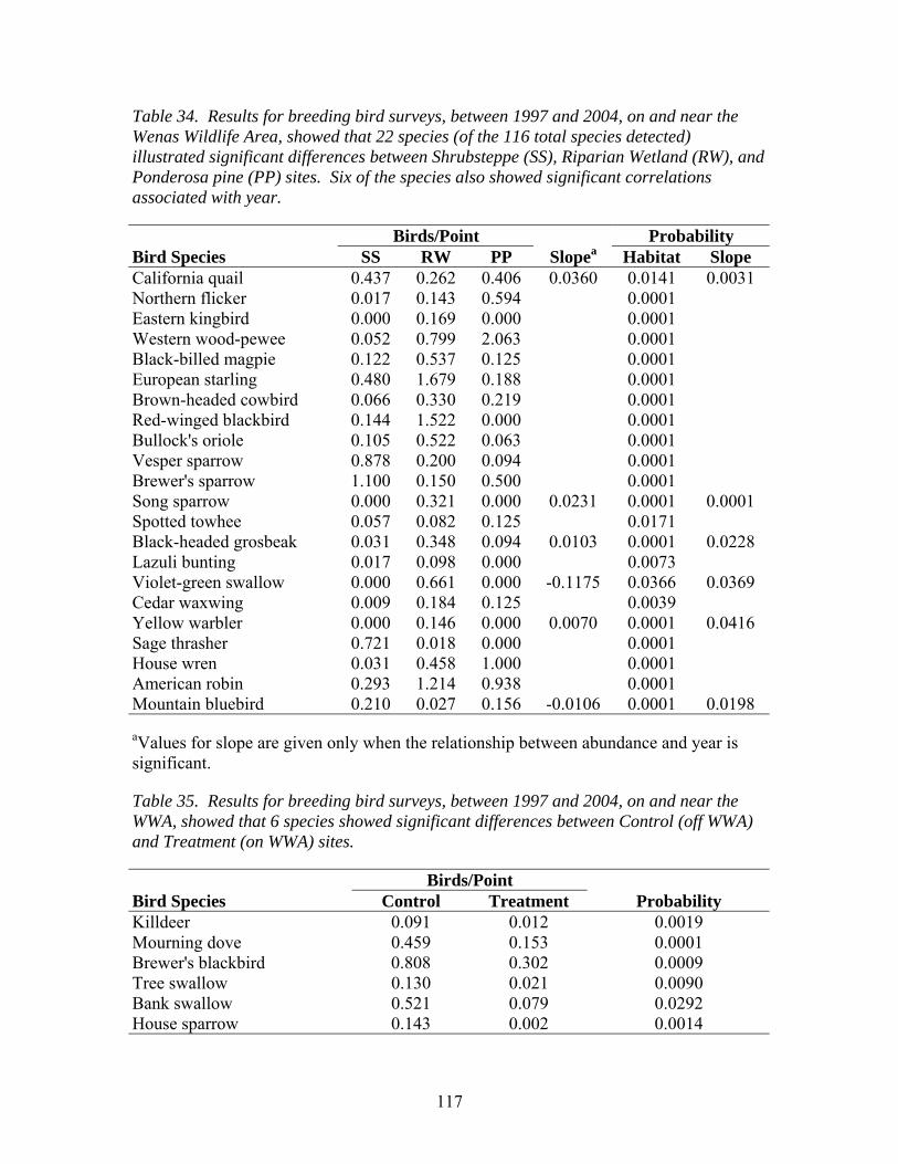
117
Table 34. Results for breeding bird surveys, between 1997 and 2004, on and near the Wenas Wildlife Area, showed that 22 species (of the 116 total species detected) illustrated significant differences between Shrubsteppe (SS), Riparian Wetland (RW), and Ponderosa pine (PP) sites. Six of the species also showed significant correlations associated with year.
Birds/Point Probability Bird Species SS RW PP Slopea Habitat Slope California quail 0.437 0.262 0.406 0.0360 0.0141 0.0031 Northern flicker 0.017 0.143 0.594 0.0001 Eastern kingbird 0.000 0.169 0.000 0.0001 Western wood-pewee 0.052 0.799 2.063 0.0001 Black-billed magpie 0.122 0.537 0.125 0.0001 European starling 0.480 1.679 0.188 0.0001 Brown-headed cowbird 0.066 0.330 0.219 0.0001 Red-winged blackbird 0.144 1.522 0.000 0.0001 Bullock's oriole 0.105 0.522 0.063 0.0001 Vesper sparrow 0.878 0.200 0.094 0.0001 Brewer's sparrow 1.100 0.150 0.500 0.0001 Song sparrow 0.000 0.321 0.000 0.0231 0.0001 0.0001 Spotted towhee 0.057 0.082 0.125 0.0171 Black-headed grosbeak 0.031 0.348 0.094 0.0103 0.0001 0.0228 Lazuli bunting 0.017 0.098 0.000 0.0073 Violet-green swallow 0.000 0.661 0.000 -0.1175 0.0366 0.0369 Cedar waxwing 0.009 0.184 0.125 0.0039 Yellow warbler 0.000 0.146 0.000 0.0070 0.0001 0.0416 Sage thrasher 0.721 0.018 0.000 0.0001 House wren 0.031 0.458 1.000 0.0001 American robin 0.293 1.214 0.938 0.0001 Mountain bluebird 0.210 0.027 0.156 -0.0106 0.0001 0.0198
aValues for slope are given only when the relationship between abundance and year is significant.
Table 35. Results for breeding bird surveys, between 1997 and 2004, on and near the WWA, showed that 6 species showed significant differences between Control (off WWA) and Treatment (on WWA) sites.
Birds/Point Bird Species Control Treatment Probability Killdeer 0.091 0.012 0.0019 Mourning dove 0.459 0.153 0.0001 Brewer's blackbird 0.808 0.302 0.0009 Tree swallow 0.130 0.021 0.0090 Bank swallow 0.521 0.079 0.0292 House sparrow 0.143 0.002 0.0014
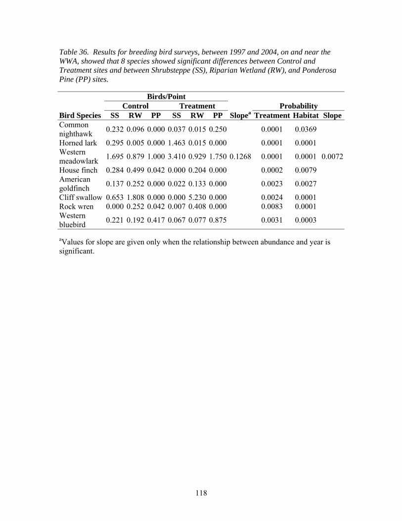
118
Table 36. Results for breeding bird surveys, between 1997 and 2004, on and near the WWA, showed that 8 species showed significant differences between Control and Treatment sites and between Shrubsteppe (SS), Riparian Wetland (RW), and Ponderosa Pine (PP) sites.
Birds/Point Control Treatment Probability Bird Species SS RW PP SS RW PP Slopea Treatment Habitat SlopeCommon nighthawk 0.232 0.096 0.000 0.037 0.015 0.250 0.0001 0.0369
Horned lark 0.295 0.005 0.000 1.463 0.015 0.000 0.0001 0.0001 Western meadowlark 1.695 0.879 1.000 3.410 0.929 1.750 0.1268 0.0001 0.0001 0.0072
House finch 0.284 0.499 0.042 0.000 0.204 0.000 0.0002 0.0079 American goldfinch 0.137 0.252 0.000 0.022 0.133 0.000 0.0023 0.0027
Cliff swallow 0.653 1.808 0.000 0.000 5.230 0.000 0.0024 0.0001 Rock wren 0.000 0.252 0.042 0.007 0.408 0.000 0.0083 0.0001 Western bluebird 0.221 0.192 0.417 0.067 0.077 0.875 0.0031 0.0003
aValues for slope are given only when the relationship between abundance and year is significant.
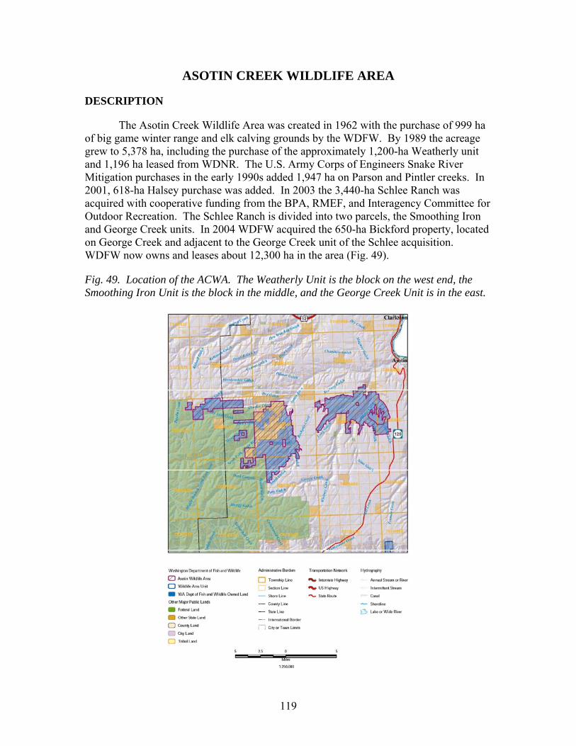
119
ASOTIN CREEK WILDLIFE AREA
DESCRIPTION
The Asotin Creek Wildlife Area was created in 1962 with the purchase of 999 ha of big game winter range and elk calving grounds by the WDFW. By 1989 the acreage grew to 5,378 ha, including the purchase of the approximately 1,200-ha Weatherly unit and 1,196 ha leased from WDNR. The U.S. Army Corps of Engineers Snake River Mitigation purchases in the early 1990s added 1,947 ha on Parson and Pintler creeks. In 2001, 618-ha Halsey purchase was added. In 2003 the 3,440-ha Schlee Ranch was acquired with cooperative funding from the BPA, RMEF, and Interagency Committee for Outdoor Recreation. The Schlee Ranch is divided into two parcels, the Smoothing Iron and George Creek units. In 2004 WDFW acquired the 650-ha Bickford property, located on George Creek and adjacent to the George Creek unit of the Schlee acquisition. WDFW now owns and leases about 12,300 ha in the area (Fig. 49).
Fig. 49. Location of the ACWA. The Weatherly Unit is the block on the west end, the Smoothing Iron Unit is the block in the middle, and the George Creek Unit is in the east.
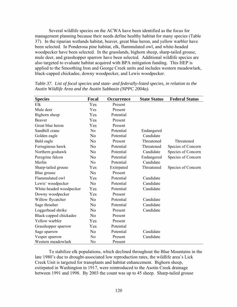
120
Several wildlife species on the ACWA have been identified as the focus for management planning because their needs define healthy habitat for many species (Table 37). In the riparian wetlands habitat, beaver, great blue heron, and yellow warbler have been selected. In Ponderosa pine habitat, elk, flammulated owl, and white-headed woodpecker have been selected. In the grasslands, bighorn sheep, sharp-tailed grouse, mule deer, and grasshopper sparrow have been selected. Additional wildlife species are also targeted to evaluate habitat acquired with BPA mitigation funding. This HEP is applied to the Smoothing Iron and George Creek units and includes western meadowlark, black-capped chickadee, downy woodpecker, and Lewis woodpecker.
Table 37. List of focal species and state- and federally-listed species, in relation to the Asotin Wildlife Area and the Asotin Subbasin (NPPC 2004a).
Species Focal Occurrence State Status Federal Status Elk Yes Present Mule deer Yes Present Bighorn sheep Yes Potential Beaver Yes Present Great blue heron Yes Present Sandhill crane No Potential Endangered Golden eagle No Potential Candidate Bald eagle No Present Threatened Threatened Ferruginous hawk No Potential Threatened Species of Concern Northern goshawk No Potential Candidate Species of Concern Peregrine falcon No Potential Endangered Species of Concern Merlin No Potential Candidate Sharp-tailed grouse Yes Extirpated Threatened Species of Concern Blue grouse No Present Flammulated owl Yes Potential Candidate Lewis’ woodpecker No Potential Candidate White-headed woodpecker Yes Potential Candidate Downy woodpecker Yes Present Willow flycatcher No Potential Candidate Sage thrasher No Potential Candidate Loggerhead shrike No Present Candidate Black-capped chickadee No Present Yellow warbler Yes Present Grasshopper sparrow Yes Potential Sage sparrow No Potential Candidate Vesper sparrow No Present Candidate Western meadowlark No Present
To stabilize elk populations, which declined throughout the Blue Mountains in the late 1980’s due to drought-associated low reproduction rates, the wildlife area’s Lick Creek Unit is targeted for transplants and habitat enhancement. Bighorn sheep, extirpated in Washington in 1917, were reintroduced to the Asotin Creek drainage between 1991 and 1998. By 2003 the count was up to 45 sheep. Sharp-tailed grouse
121
historically occupied the grasslands and shrubsteppe habitats of the wildlife area (Fig. 1). There have been no confirmed sightings of the species for decades, due to alteration of native habitat, the Smoothing Iron Unit includes potentially high-quality grouse habitat and WDFW is assessing potential enhancements that may restore a viable population of these native grouse. Mountain quail have been extirpated from eastern Washington. Mountain quail were recently translocated to ACWA in an effort to re-establish a population.
Numerous strategies are being considered and applied on the ACWA. These include: 1) Reduce road densities; 2) Alter forestry practices to restore wildlife-friendly habitat; 3) Reduce and/or alter livestock grazing; 4) Restore habitat by planting native vegetation; 5) Control noxious weeds; 6) Controlled burns to improve habitat; and 7) Reduce disturbance by people in wildlife-critical areas; 8) Use fences to protect key habitats.
ASOTIN SUBBASIN
The NPPC (2004a) recommends specific strategies to address habitat and biological objectives in focal habitats; Ponderosa Pine, interior grasslands, and interior riparian wetlands. While all habitats are important, these focal habitats were selected in part because they are disproportionately vulnerable to anthropogenic impacts, and likely have received the highest level of impacts within the subbasin, and in adjacent subbasins. Some of the identified impacts are, for all practical purposes, irreversible and others are already being mitigated through ongoing management. Although many focal species are considered within these focal habitats (Table 37), only those in habitats on ACWA are considered here including: 1) Mule deer, bighorn sheep, grasshopper sparrow, and sharp-tailed grouse in interior grasslands; 2) Yellow warbler, American beaver, and great blue heron in interior riparian wetlands; and 3) White-headed woodpecker, flammulated owl, and elk in Ponderosa pine.
The NPPC (2004a) recommends the development of an integrated monitoring program that influences adaptive management. The NPPC also recommends selection of a survey protocol to measure the abundance of focal species (Table 37) and to measure diversity and richness of species assemblages within each habitat type. In certain cases, this could include the evaluation of population status for each focal species in each focal habitat type. In addition, the NPPC (2004a) recommends inventory of other grassland, riparian wetland, and Ponderosa pine obligates in an effort to test assumptions of the umbrella species concept.
MONITORING AND EVALUATION
Habitat
HEP transects were conducted on the ACWA between 2003 and 2004 on the George Creek (Fig. 50) and Asotin Creek (Fig. 51) units. The coverage of the ACWA was relatively complete when compared to other areas and the compilation of data is much better organized. This was due, in part, to the refinement of methods over time.

122
Fig. 50. George Creek Unit of the ACWA showing the distribution of HEP transects.
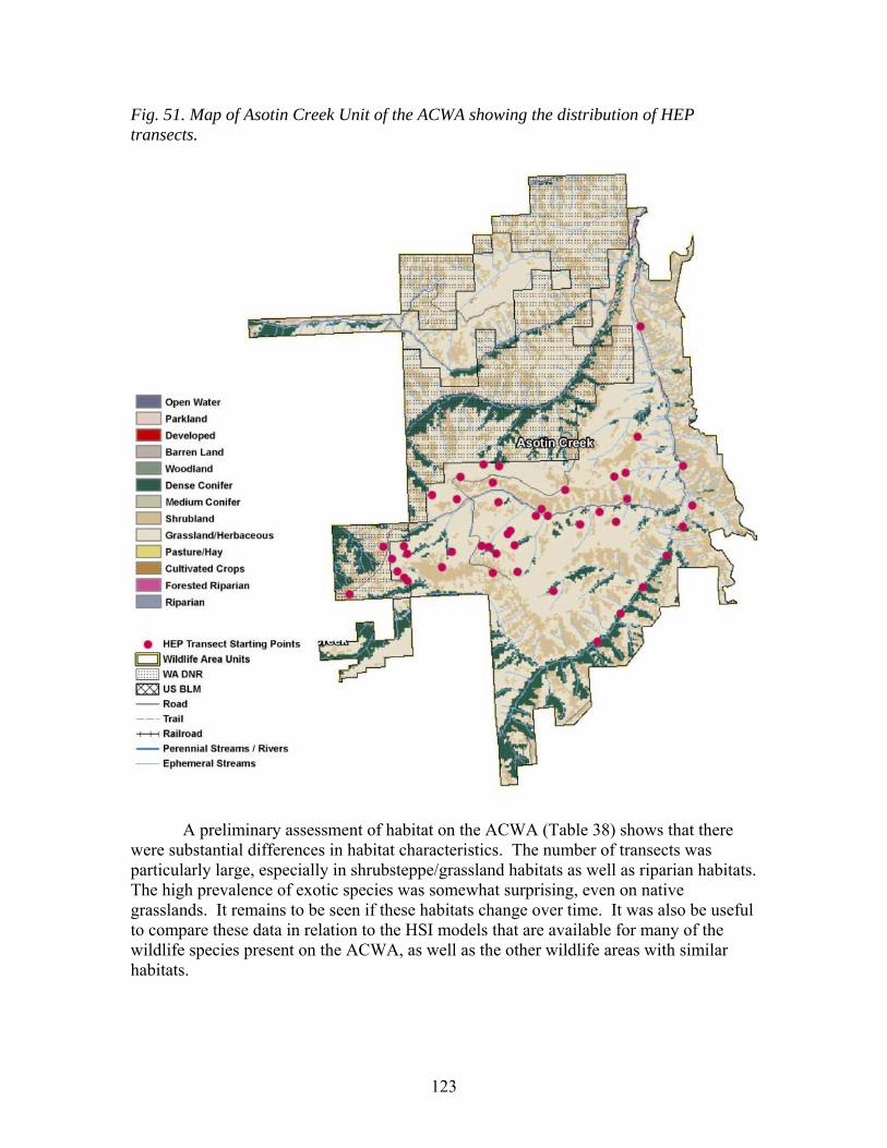
123
Fig. 51. Map of Asotin Creek Unit of the ACWA showing the distribution of HEP transects.
A preliminary assessment of habitat on the ACWA (Table 38) shows that there were substantial differences in habitat characteristics. The number of transects was particularly large, especially in shrubsteppe/grassland habitats as well as riparian habitats. The high prevalence of exotic species was somewhat surprising, even on native grasslands. It remains to be seen if these habitats change over time. It was also be useful to compare these data in relation to the HSI models that are available for many of the wildlife species present on the ACWA, as well as the other wildlife areas with similar habitats.
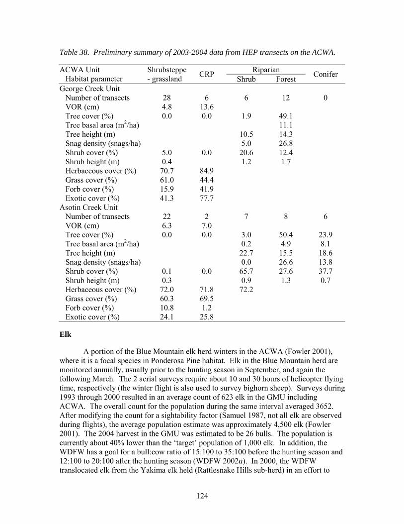
124
Table 38. Preliminary summary of 2003-2004 data from HEP transects on the ACWA.
Riparian ACWA Unit Habitat parameter
Shrubsteppe - grassland CRP Shrub Forest Conifer
George Creek Unit Number of transects 28 6 6 12 0 VOR (cm) 4.8 13.6 Tree cover (%) 0.0 0.0 1.9 49.1 Tree basal area (m2/ha) 11.1 Tree height (m) 10.5 14.3 Snag density (snags/ha) 5.0 26.8 Shrub cover (%) 5.0 0.0 20.6 12.4 Shrub height (m) 0.4 1.2 1.7 Herbaceous cover (%) 70.7 84.9 Grass cover (%) 61.0 44.4 Forb cover (%) 15.9 41.9 Exotic cover (%) 41.3 77.7 Asotin Creek Unit Number of transects 22 2 7 8 6 VOR (cm) 6.3 7.0 Tree cover (%) 0.0 0.0 3.0 50.4 23.9 Tree basal area (m2/ha) 0.2 4.9 8.1 Tree height (m) 22.7 15.5 18.6 Snag density (snags/ha) 0.0 26.6 13.8 Shrub cover (%) 0.1 0.0 65.7 27.6 37.7 Shrub height (m) 0.3 0.9 1.3 0.7 Herbaceous cover (%) 72.0 71.8 72.2 Grass cover (%) 60.3 69.5 Forb cover (%) 10.8 1.2 Exotic cover (%) 24.1 25.8
Elk
A portion of the Blue Mountain elk herd winters in the ACWA (Fowler 2001), where it is a focal species in Ponderosa Pine habitat. Elk in the Blue Mountain herd are monitored annually, usually prior to the hunting season in September, and again the following March. The 2 aerial surveys require about 10 and 30 hours of helicopter flying time, respectively (the winter flight is also used to survey bighorn sheep). Surveys during 1993 through 2000 resulted in an average count of 623 elk in the GMU including ACWA. The overall count for the population during the same interval averaged 3652. After modifying the count for a sightability factor (Samuel 1987, not all elk are observed during flights), the average population estimate was approximately 4,500 elk (Fowler 2001). The 2004 harvest in the GMU was estimated to be 26 bulls. The population is currently about 40% lower than the ‘target’ population of 1,000 elk. In addition, the WDFW has a goal for a bull:cow ratio of 15:100 to 35:100 before the hunting season and 12:100 to 20:100 after the hunting season (WDFW 2002a). In 2000, the WDFW translocated elk from the Yakima elk held (Rattlesnake Hills sub-herd) in an effort to
125
bolster productivity. Results for this effort are not available yet. The WDFW plans to continue conducting annual surveys of the Blue Mountain elk herd.
Mule Deer
Mule deer are present on the ACWA, and are considered a focal species in shrubsteppe. Surveys are regularly conducted in the region, not specifically associated with the ACWA, to monitor populations and harvest. Both aerial and ground surveys are used to monitor populations and sex ratio (WDFW 2002a, 2003). Surveys are conducted before and after the harvest, and sightability is considered in the population estimates. Check stations and questionnaires are also used to estimate the harvest. The GMU containing the ACWA had an estimated harvest of 40 bucks in 2004. Population and harvest estimates are not specifically available for the ACWA.
Bighorn Sheep
The bighorn sheep associated with the ACWA is the Rocky Mountain subspecies. Although it is not considered a focal species, it is clearly important enough to warrant annual surveys. Aerial or ground surveys are used to monitor and evaluate bighorn sheep populations (WDFW 2002a, 2003) in the area, on and off the WWA. Surveys are usually conducted during lambing or rutting periods and data are used to estimate lamb recruitment, sex ratio, adult survival, population size, and percentage of mature rams in the population. The 2002 population on the ACWA was estimated to be 38, with a target population of 50 to 60. The population is not harvested.
Great Blue Heron
There are two known nesting colonies supporting about 21-23 nests in total for great blue herons in the WWS (Ashley and Stovall 2004b). However, neither colony is near the ACWA. Nevertheless, because the great blue heron is a focal species, efforts to monitor these colonies should continue.
Prairie Grouse
The ACWA is in the historic range of sharp-tailed grouse, but long-term declines in distribution and populations appear to have eliminated most sharp-tailed grouse from the region. Nevertheless, there have been occasional observations (difficult to confirm) of sharp-tailed grouse on the ACWA. Because there have been translocations of sharp-tailed grouse in northeastern Oregon and there is a population about 50 km away in Idaho, these possible observations should be seriously considered. Annual surveys of prairie grouse are conducted in Washington and should be able to detect a range expansion if it occurs. Additional efforts should include the area on, and near, the ACWA.
General Bird Surveys
The USGS has a breeding bird survey (Cloverland, number 84, Fig. 27) that traverses the ACWA for about 21 of its 50 points (some ‘treatment’ points on, and some
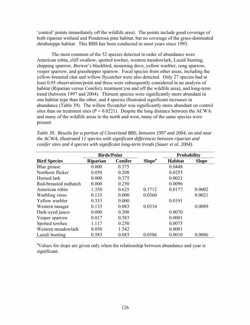
126
‘control’ points immediately off the wildlife area). The points include good coverage of both riparian wetland and Ponderosa pine habitat, but no coverage of the grass-dominated shrubsteppe habitat. This BBS has been conducted in most years since 1993.
The most common of the 52 species detected in order of abundance were American robin, cliff swallow, spotted towhee, western meadowlark, Lazuli bunting, chipping sparrow, Brewer’s blackbird, mourning dove, yellow warbler, song sparrow, vesper sparrow, and grasshopper sparrow. Focal species from other areas, including the yellow-breasted chat and willow flycatcher were also detected. Only 27 species had at least 0.05 observations/point and these were subsequently considered in an analysis of habitat (Riparian versus Conifer), treatment (on and off the wildlife area), and long-term trend (between 1997 and 2004). Thirteen species were significantly more abundant in one habitat type than the other, and 4 species illustrated significant increases in abundance (Table 39). The willow flycatcher was significantly more abundant on control sites than on treatment sites (P = 0.0221). Despite the long distance between the ACWA and many of the wildlife areas to the north and west, many of the same species were present.
Table 39. Results for a portion of Cloverland BBS, between 1997 and 2004, on and near the ACWA, illustrated 11 species with significant differences between riparian and conifer sites and 4 species with significant long-term trends (Sauer et al. 2004).
Birds/Point Probability Bird Species Riparian Conifer Slopea Habitat Slope Blue grouse 0.000 0.375 0.0448 Northern flicker 0.050 0.208 0.0255 Horned lark 0.000 0.375 0.0021 Red-breasted nuthatch 0.000 0.250 0.0096 American robin 1.350 0.625 0.1712 0.0177 0.0002 Warbling vireo 0.133 0.000 0.0360 0.0021 Yellow warbler 0.333 0.000 0.0191 Western tanager 0.133 0.083 0.0334 0.0089 Dark-eyed junco 0.000 0.208 0.0070 Vesper sparrow 0.017 0.583 0.0001 Spotted towhee 1.117 0.250 0.0075 Western meadowlark 0.050 1.542 0.0001 Lazuli bunting 0.583 0.083 0.0586 0.0010 0.0086
aValues for slope are given only when the relationship between abundance and year is significant.
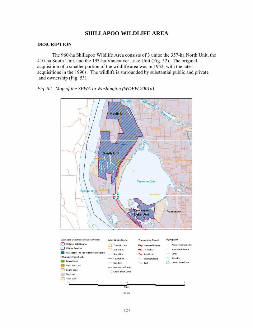
127
SHILLAPOO WILDLIFE AREA
DESCRIPTION
The 960-ha Shillapoo Wildlife Area consists of 3 units: the 357-ha North Unit, the 410-ha South Unit, and the 193-ha Vancouver Lake Unit (Fig. 52). The original acquisition of a smaller portion of the wildlife area was in 1952, with the latest acquisitions in the 1990s. The wildlife is surrounded by substantial public and private land ownership (Fig. 53).
Fig. 52. Map of the SPWA in Washington (WDFW 2001a).

128
Fig. 53. Land ownership in the vicinity of the Shillapoo Wildlife Area in Washington (WDFW 2001a).
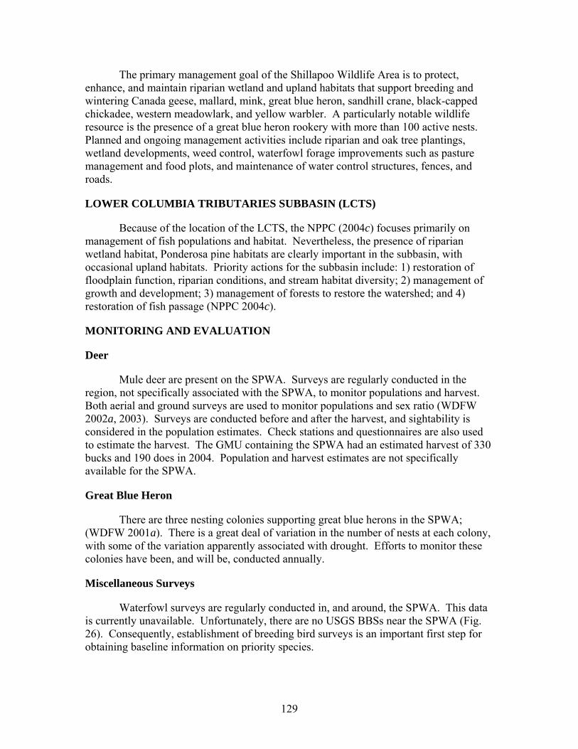
129
The primary management goal of the Shillapoo Wildlife Area is to protect, enhance, and maintain riparian wetland and upland habitats that support breeding and wintering Canada geese, mallard, mink, great blue heron, sandhill crane, black-capped chickadee, western meadowlark, and yellow warbler. A particularly notable wildlife resource is the presence of a great blue heron rookery with more than 100 active nests. Planned and ongoing management activities include riparian and oak tree plantings, wetland developments, weed control, waterfowl forage improvements such as pasture management and food plots, and maintenance of water control structures, fences, and roads.
LOWER COLUMBIA TRIBUTARIES SUBBASIN (LCTS)
Because of the location of the LCTS, the NPPC (2004c) focuses primarily on management of fish populations and habitat. Nevertheless, the presence of riparian wetland habitat, Ponderosa pine habitats are clearly important in the subbasin, with occasional upland habitats. Priority actions for the subbasin include: 1) restoration of floodplain function, riparian conditions, and stream habitat diversity; 2) management of growth and development; 3) management of forests to restore the watershed; and 4) restoration of fish passage (NPPC 2004c).
MONITORING AND EVALUATION
Deer
Mule deer are present on the SPWA. Surveys are regularly conducted in the region, not specifically associated with the SPWA, to monitor populations and harvest. Both aerial and ground surveys are used to monitor populations and sex ratio (WDFW 2002a, 2003). Surveys are conducted before and after the harvest, and sightability is considered in the population estimates. Check stations and questionnaires are also used to estimate the harvest. The GMU containing the SPWA had an estimated harvest of 330 bucks and 190 does in 2004. Population and harvest estimates are not specifically available for the SPWA.
Great Blue Heron
There are three nesting colonies supporting great blue herons in the SPWA; (WDFW 2001a). There is a great deal of variation in the number of nests at each colony, with some of the variation apparently associated with drought. Efforts to monitor these colonies have been, and will be, conducted annually.
Miscellaneous Surveys
Waterfowl surveys are regularly conducted in, and around, the SPWA. This data is currently unavailable. Unfortunately, there are no USGS BBSs near the SPWA (Fig. 26). Consequently, establishment of breeding bird surveys is an important first step for obtaining baseline information on priority species.
130
DESERT WILDLIFE AREA
DESCRIPTION
The Desert Wildlife Area is about 14,200 ha in size (Fig. 54). Because the natural basin currently serves as a collector for irrigation water from upslope farmlands, the DWA supports a mosaic of shrubsteppe and riparian vegetation. The thousands of small lakes, potholes, and seeps support Canada geese, swans, and numerous species of waterfowl. In addition, shorebirds are common as well as Caspian tern, American white pelican, sandhill crane, ring-billed gull, great blue heron, and western meadowlark. Management is designed to support these species as well as to reduce the negative effects of introduced vegetation such as Russian olive.
Fig. 54. Location of the Desert Wildlife Area in Washington.
131
CRAB CREEK SUBBASIN
The NPPC (2004b) recommends specific strategies to address habitat and biological objectives in three focal habitats; shrubsteppe, riparian wetland, and Ponderosa pine. However, Ponderosa pine is essentially absent from the DWA. While all habitats are important, these focal habitats were selected in part because they are disproportionately vulnerable to anthropogenic impacts, and likely have received the highest level of impacts within the subbasin. Some of the identified impacts are, for all practical purposes, irreversible and others are already being mitigated through ongoing management. Many focal species are considered within these focal habitats including: 1) sharp-tailed grouse, greater sage-grouse, mule deer, sage thrasher, and pygmy rabbit in shrubsteppe; and 2) red-eyed vireo, yellow-breasted chat, and American beaver in riparian wetlands.
The NPPC (2004b) recommends the development of an integrated monitoring program that influences adaptive management. The NPPC also recommends selection of a survey protocol to measure the abundance of focal species and to measure diversity and richness of species assemblages within each habitat type. In certain cases, this could include the evaluation of population status for each focal species in each focal habitat type. In addition, the NPPC (2004b) recommends inventory of other shrubsteppe, riparian wetland, and Ponderosa pine obligates in an effort to test assumptions of the umbrella species concept.
MONITORING AND EVALUATION
Habitat
Six HEP transects were conducted on the DWA in 1998. Only one habitat, shrubsteppe, was sampled. The average shrub cover was 22.1% and the average shrub height was 0.7 m. It is not certain at this stage if all the data that has been collected is currently available. Data management for the DWA and all other wildlife areas will be an ongoing process.
Deer
Mule deer are present on the DWA in low numbers. Surveys are regularly conducted in the region, not specifically associated with the DWA, to monitor populations and harvest. Both aerial and ground surveys are used to monitor populations and sex ratio (WDFW 2002a, 2003). Surveys are conducted before and after the harvest, and sightability is considered in the population estimates. Check stations and questionnaires are also used to estimate the harvest. Because the goal has been to increase the number of deer in the GMU associated with DWA, the harvest on the area has been negligible, if not absent.
Great Blue Heron
There are known nesting colonies supporting great blue herons on the DWA. There is a great deal of variation in the number of nests at each colony, with some of the

132
variation apparently associated with drought. Efforts to monitor these colonies have been, and will be, conducted annually.
Miscellaneous Surveys
Waterfowl surveys are regularly conducted in, and around, the DWA. This data is currently unavailable. The DWA is the historic range of greater sage-grouse and sharp-tailed grouse, but long-term declines in distribution and abundance have left the region essentially empty of prairie grouse. Lek surveys are done annually in all areas with known populations. Regular surveys for Washington ground squirrels are also conducted. There is a USGS BBSs the skirts the southern edge of the DWA, but it is not clear at this state if the data will be useful.
133
DISCUSSION AND RECOMENDATIONS
Monitoring and evaluation of wildlife and the habitats upon which they depend are the basis for adaptive management decisions. Without a foundation of information, management can be applied, but it cannot be adjusted to meet evolving situations or improvements in knowledge. Although guidelines for management are clearly beyond the scope of this report, the needs, designs, and application of monitoring and evaluation information is the purpose of this report. This overview is only meant to provide a starting point in this process, because, like the adaptive nature of management, monitoring and evaluation activities should also be flexible enough that they can be modified to fulfill requirements that are, as of now, unanticipated.
To a certain extent, this report represents an early effort to bring together the available data on monitoring and evaluation for BPA-funded wildlife areas. This type of effort is critical in the long-term effort to monitor and evaluate management on wildlife areas. Without a unified and coherent effort to standardize, gather, manage, interpret, and evaluate data on wildlife populations and their habitats, it will be virtually impossible to ensure the cost-effectiveness of management. Although there is no way to be certain that every management decision will be the correct one, without good and accessible data on wildlife populations and the habitats upon which they depend, there will be no realistic way to improve management when it is not on target.
There are many examples of uncoordinated collection of data throughout eastern Washington. There are examples of ‘lost’ habitat photographs, misplaced data files, habitat plots that cannot be re-located, and haphazard and miscellaneous surveys that cannot be understood and/or replicated. These problems are exacerbated by numerous well-intentioned individuals that understand the importance of good data, but are unable or are poorly positioned to apply adequate data-collection standards on the scale needed. Similarly, it is probably unreasonable to expect wildlife area managers to be able to manage 20,000 ha of habitat, and be able to conduct regular wildlife and habitat surveys, have their data be comparable to the data collected 10 years before, and have their data be comparable to the data collected on different wildlife areas.
There is an underlying assumption that focal species reflect a broader group of species that responds similarly to changes in key features of the habitat. Hence, it is essential that these relationships be examined. Much of the current information on these relationships is based on untested assumptions. For example, because the shrubsteppe landscape and habitat appears to be ‘simple’ in appearance and structure, some might believe that shrubsteppe obligates would respond in similar ways to the changes in basic characteristics in the shrubsteppe habitat (shrub cover, grass cover, grass height, plant diversity). However, these relationships are often untested. This is perhaps the biggest reason why these systems should be monitored. Because we cannot always be certain of the wildlife response to changes in the environment, data must be collected to document those changes and the wildlife response to the changes. It is also clear that shrubsteppe obligates respond to different characteristics, even in the relatively simple shrubsteppe habitat; as illustrated by the previously discussed continuum of sparrows (Dobler et al. 1996, Vander Haegen et al. 2000).
134
Based on preliminary results from this research, it may be worth considering a modified set of focal species on BPA-funded wildlife areas. Criteria for selection of focal species included their use of critical features of the habitat that reflected the needs of the larger community dependent on their particular focal habitat. These species should respond positively to improvements and negatively to habitat degradation. Based on the preliminary results and published literature for the region, it may be possible to reconsider which focal species are used in these focal habitats.
Shrubsteppe is one of the highest priority habitats in the Columbia Basin, and a focal habitat in almost every subbasin in which it is present. This is also true for the BPA-funded wildlife areas in Washington. Each wildlife area lists a set of focal species for monitoring and evaluation of shrubsteppe habitat. The list includes: bighorn sheep, mule deer, sharp-tailed grouse, greater sage-grouse, sage thrasher, grasshopper sparrow, Brewer’s sparrow, sage sparrow. Unfortunately, the same species are not focal species on all wildlife areas (Table 2). The monitoring and evaluation of wildlife areas will be more effective if a similar set of focal species is used by each wildlife area. In this case, this listed set of focal species (with the additional of savannah and vesper sparrow) would offer an excellent opportunity to evaluate the wildlife response to habitat characteristics in shrubsteppe habitat. The reason for this is that these species are all relatively common in the Columbia Basin and they appear to respond to different characteristics in the shrubsteppe (Vander Haegen et al. 2004b, 2005b). For example, 5 sparrows fit on an approximate continuum of sagebrush-dominated to grass-dominated shrubsteppe; sage sparrow, Brewer’s sparrow, vesper sparrow, savannah sparrow, and grasshopper sparrow (in order). Consequently, the relative proportion of each type of sparrow can provide support for the types of other species present in the system and the specific characteristics of the habitat.
Greater sage-grouse and sharp-tailed grouse are examples of species that are problematic with regard to monitoring and evaluation of habitat-based objectives. First, they have big ranges, low densities and they are difficult to adequately monitor. Consequently, their use or avoidance of particular areas and/or habitats is difficult to verify with actual data. Second, the prairie grouse tend to be long lived, with relatively low productivity, and delayed maturation (particularly in males). Hence, population-level response to changes in the environment can be difficult to detect because of time lags. Third, both species of prairie grouse have been extirpated from many areas in the state, thus making their response to habitat change impossible to detect. Although one could hope for range expansion into habitats that have been improved, widespread habitat fragmentation outside of the primary core habitats has made a naturally occurring range expansion virtually impossible. Translocations of birds from healthy populations to unoccupied habitats, in an effort to re-establish a population, can be attempted, but they require substantial resources. Fourth, in populations of prairie grouse that have declined to extremely low levels, a positive response to improved habitat conditions may not occur for reasons other than confusion about their habitat requirements and/or the presumed availability of suitable habitats. Research on isolated and/or small populations of prairie grouse has shown that they may be susceptible to inbreeding depression. An influx of new birds from ‘healthy’ populations has had a positive effect in some areas, including north-central Washington.
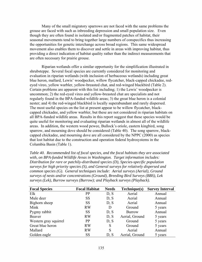
135
Many of the small migratory sparrows are not faced with the same problems the grouse are faced with such as inbreeding depression and small population size. Even though they are often found in isolated and/or fragmented patches of habitat, their seasonal movements tend to bring together large numbers of conspecifics thus increasing the opportunities for genetic interchange across broad regions. This same widespread movement also enables them to discover and settle in areas with improving habitat, thus providing a direct indication of habitat quality rather than the indirect measurements that are often necessary for prairie grouse.
Riparian wetlands offer a similar opportunity for the simplification illustrated in shrubsteppe. Several focal species are currently considered for monitoring and evaluation in riparian wetlands (with inclusion of herbaceous wetlands) including great blue heron, mallard, Lewis’ woodpecker, willow flycatcher, black-capped chickadee, red-eyed vireo, yellow warbler, yellow-breasted chat, and red-winged blackbird (Table 2). Certain problems are apparent with this list including; 1) the Lewis’ woodpecker is uncommon; 2) the red-eyed vireo and yellow-breasted chat are specialists and not regularly found in the BPA-funded wildlife areas; 3) the great blue heron is a colonial nester; and 4) the red-winged blackbird is locally superabundant and rarely dispersed. The most useful species on the list at present appear to be willow flycatcher, black-capped chickadee, and yellow warbler, but these are not considered in riparian habitats on all BPA-funded wildlife areas. Results in this report suggest that these species would be quite useful for monitoring and evaluating riparian wetlands in almost all of the wildlife areas. In addition, the western wood pewee, Bullock’s oriole, eastern kingbird, song sparrow, and mourning dove should be considered (Table 40). The song sparrow, black-capped chickadee, and mourning dove are all considered by the NPPC (2000) as species that lost habitat due to the construction and operation federal hydrosystems in the Columbia Basin (Table 1).
Table 40. Recommended list of focal species, and the focal habitats they are associated with, on BPA-funded Wildlife Areas in Washington. Target information includes: Distribution for rare or patchily-distributed species (D), Species-specific population surveys for high priority species (S), and General surveys for relatively dispersed and common species (G). General techniques include: Aerial surveys (Aerial), Ground surveys of nests and/or concentrations (Ground), Breeding Bird Surveys (BBS), Lek surveys (Lek), Burrow surveys (Burrow); and Playback surveys (Playback).
Focal Species Focal Habitat Needs Technique(s) Survey IntervalElk PP D, S Aerial Annual Mule deer SS D, S Aerial Annual Bighorn sheep SS D, S Aerial Annual Mink RW D Ground 5 years Pygmy rabbit SS D, S Burrow Annual Beaver RW D, S Aerial, Ground 5 years Western gray squirrel PP D, S Ground 5 years Great blue heron RW S Ground 5 years Mallard RW S Aerial Annual Golden eagle SS D, S Aerial, Ground 5 years
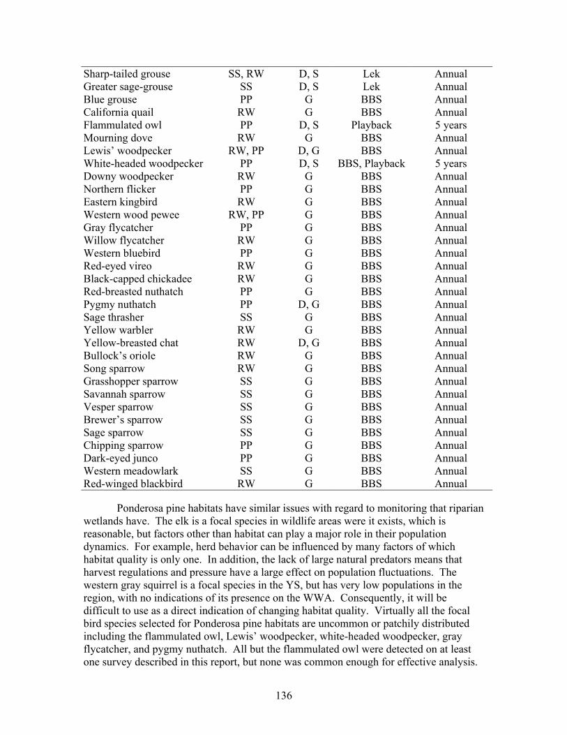
136
Sharp-tailed grouse SS, RW D, S Lek Annual Greater sage-grouse SS D, S Lek Annual Blue grouse PP G BBS Annual California quail RW G BBS Annual Flammulated owl PP D, S Playback 5 years Mourning dove RW G BBS Annual Lewis’ woodpecker RW, PP D, G BBS Annual White-headed woodpecker PP D, S BBS, Playback 5 years Downy woodpecker RW G BBS Annual Northern flicker PP G BBS Annual Eastern kingbird RW G BBS Annual Western wood pewee RW, PP G BBS Annual Gray flycatcher PP G BBS Annual Willow flycatcher RW G BBS Annual Western bluebird PP G BBS Annual Red-eyed vireo RW G BBS Annual Black-capped chickadee RW G BBS Annual Red-breasted nuthatch PP G BBS Annual Pygmy nuthatch PP D, G BBS Annual Sage thrasher SS G BBS Annual Yellow warbler RW G BBS Annual Yellow-breasted chat RW D, G BBS Annual Bullock’s oriole RW G BBS Annual Song sparrow RW G BBS Annual Grasshopper sparrow SS G BBS Annual Savannah sparrow SS G BBS Annual Vesper sparrow SS G BBS Annual Brewer’s sparrow SS G BBS Annual Sage sparrow SS G BBS Annual Chipping sparrow PP G BBS Annual Dark-eyed junco PP G BBS Annual Western meadowlark SS G BBS Annual Red-winged blackbird RW G BBS Annual
Ponderosa pine habitats have similar issues with regard to monitoring that riparian wetlands have. The elk is a focal species in wildlife areas were it exists, which is reasonable, but factors other than habitat can play a major role in their population dynamics. For example, herd behavior can be influenced by many factors of which habitat quality is only one. In addition, the lack of large natural predators means that harvest regulations and pressure have a large effect on population fluctuations. The western gray squirrel is a focal species in the YS, but has very low populations in the region, with no indications of its presence on the WWA. Consequently, it will be difficult to use as a direct indication of changing habitat quality. Virtually all the focal bird species selected for Ponderosa pine habitats are uncommon or patchily distributed including the flammulated owl, Lewis’ woodpecker, white-headed woodpecker, gray flycatcher, and pygmy nuthatch. All but the flammulated owl were detected on at least one survey described in this report, but none was common enough for effective analysis.
137
Relatively common species that could be considered include dusky grouse, northern flicker, western wood pewee, red-breasted nuthatch, western bluebird, dark-eyed junco, and chipping sparrow. For example, the dusky grouse was considered by the NPPC (2000) as a species that lost habitat due to the construction and operation federal hydrosystems in the Columbia Basin (Table 1).
When considered in total, it is probably useful to broaden the list of focal species (Table 40). The reasons for this increase can be summarized with some basic generalities. First, not all species are present and/or common enough to permit analysis of data on distribution and abundance. This lack of data makes it difficult to test assumptions about established habitat suitability models and therefore eliminates the opportunity for adaptive management. Second, broadening the list of focal species helps to direct monitoring and evaluation attention toward a larger suite of habitat characteristics, rather than a few parameters that pertain to a small number of suitability models. This is extremely important in that, future research may illustrate a need for data that would otherwise not be collected. Third, a longer list of species better enables the testing of assumptions about the usefulness of focal species for providing insights into the integrity of the larger ecological system to which they belong. Fourth, more focal species increases the opportunity for comparison between different wildlife areas and the species and habitats that they share. Hence, the ‘lessons’ learned at SLWA may be applied at the SFWA.
One of the major problems with an extended list of focal species is that there are few species with established habitat suitability models. In this case establishment of an H.S.I. can refer to a number of stages including: 1) development of a working suitability model; 2) publication of a peer-reviewed HSI; 3) testing of an HSI with independently-collected data; and 4) establishment of the validity of the HSI in the specific area of interest. There are few, if any, models that meet the most stringent of these stages. Current HSI procedures are based on the best information available, sometimes from different regions and/or situations. As new information becomes available, there should be a periodic re-evaluation of existing HSIs to verify that the target species of wildlife is responding to habitat change as predicted. This information on the wildlife species (based on monitoring) should be linked with information on the underlying habitat.
Care should be taken in this HSI evaluation process. Wildlife species can respond in unexpected ways that may, or may not, directly reflect the underlying habitat. In simple situations, the response of a species is directly and immediately related to characteristics of the habitat. As the habitat changes, the dependent species responds quickly to the new conditions. However, most species are influenced by more than underlying habitat, or at the least more than the baseline habitat characteristics were are capable of measuring. Two focal species, the greater sage-grouse and sharp-tailed grouse, appear to be more complex than the current HSI procedures would suggest. Information from other regions has indicated that small and relatively isolated populations may encounter genetic bottlenecks, and that they may eventually suffer declines in productivity as a result (Westemeier et al. 1998, Johnson et al. 2003). The prairie grouse populations in Washington are clearly in the size range, where problems of this sort may be expected. This is the fundamental reason why populations of both
138
species are current being augmented with grouse from ‘healthy’ populations. It is also an explanation for how monitoring and evaluation data and adaptive management can be applied. For example, information on the distribution and abundance of prairie grouse in Washington has been collected since the 1950s (Schroeder et al. 2000a, 2000b). In the early 1990s following the acquisition of the SCWA and SLWA, and altered management on the YTC, populations of both species failed to improve in ways predicted with current HSI models. The subsequently application of genetic information to the issue (Warheit and Schroeder 2003) suggested that the ‘problem’ may not have been with the habitat, but with underlying characteristics in the birds, themselves. The WDFW (and others) responded to the new information by translocating sharp-tailed grouse to the SCWA. Sharp-tailed grouse subsequently responded with increased populations and distribution in the area around the SCWA. Similar translocations are now underway at SFWA and SLWA.
In the context of model testing, some habitat data collected to date has illustrated a basic flaw. It may have been collected with specific reference to one or two focal species in a single focal habitat. Consequently, the data collected tends to be situation specific rather than directed toward the broader questions of healthy ecosystems. For example, a particular characteristic of a habitat may not be measured if the HSI for a focal species in that habitat does not use that data. As a result, it is not always possible to use ‘old’ data to test new models about wildlife abundance, because the ‘old’ data may not be complete. The advantage of the targeted system that has been used is that it is much more efficient with regard to time. The disadvantage is that it is not as versatile or adaptive. In other words, if the H.S.I. and/or the focal species change, then data may be needed which was not collected.
As a result of these considerations, we believe that future habitat evaluation procedures should be modified to provide consistent types of data, regardless of the particular models being addressed (see earlier section on modified habitat assessment). This does not mean that the models should not be considered, but that the habitat data should be substantial enough to be applicable to multiple species and models. Because the types of data required tend to be relatively consistent for the suitability models, we do not see this as being a major problem. The advantage is that the consistency will permit the development and testing of additional models, thus strengthening the overall process.
In addition to a modification in the general philosophy concerning collection of habitat data, we also recommend focusing on habitat collection methods centered around points rather than transects. One of the problems with transects is that they cover broad areas, thus necessitating course changes to avoid habitat changes. Even when a long transect remains in a relatively consistent habitat, the risk of supple changes in habitat over a long distance may be quite large. In contrast points are easy to randomly or systematically place, and relatively easy to sample. The same tools that are used with transects (e.g., line or point intercept transects, Robel pole readings, Daubenmire plots) would also be used with the central point.
This report is clearly not the end-product in this monitoring and evaluation effort, but rather a first phase. An important task to be accomplished is the continued
139
compilation and coordination of existing data. It is only with a thorough assessment of previously collected data that appropriate decisions can be made concerning the direction of future monitoring and evaluation efforts. Retrospective analysis helps to set the stage for future monitoring and evaluation efforts on the wildlife areas. These monitoring and evaluation efforts should effectively utilize resources and be scientifically defendable. Accomplishing this will be difficult, but will provide the most certain way for the BPA to achieve its mitigation goals, while at the same time insuring the enhancement of the habitats necessary to support wildlife in the state of Washington.
A second phase is planned for the future; the purpose of which would be to provide a detailed monitoring and evaluation plan for BPA-funded wildlife areas. The first part of the future report will include habitat definitions based on the National Vegetation Classification Standard. This standard includes an established hierarchical system of 8 general classes with an increasing number of subclasses. There are approximately 75 habitat types on WDFW land and 33 habitat types consisting of at least 1000 acres. The second part of the report will include detailed maps of the wildlife areas with habitat delineations that correspond to the pre-defined habitat types. It is important that the definitions correspond to the maps so that subsequent habitat and wildlife assessments will be possible. The third part of the Phase 2 report will include a detailed protocol for monitoring and evaluation of habitat. The foundation will be a stratified-random sampling system with some opportunity to link future efforts will past efforts (primary Habitat Evaluation Procedures). The planned methods for assessing habitat have been establish and will likely focus more on random points, rather than transects. The fourth part of the report will include a detailed protocol for monitoring and evaluating wildlife.
140
LITERATURE CITED
Allen, A. W. 1982a. Habitat suitability index models: fox squirrel. U.S. Fish and Wildlife Service. FWS/OBS-82/10.18.
Allen, A. W. 1982b. Habitat suitability index models: marten. U.S. Fish and Wildlife Service. FWS/OBS-82/10.11.
Allen, A. W. 1983a. Habitat suitability index models: beaver. U.S. Fish and Wildlife Service. FWS/OBS-82/10.30. Revised.
Allen, A. W. 1983b. Habitat suitability index models: fisher. U.S. Fish and Wildlife Service. FWS/OBS-82/10.45.
Allen, A. W. 1984a. Habitat suitability index models: gray partridge. U.S. Fish and Wildlife Service. FWS/OBS-82/10.73.
Allen, A. W. 1984b. Habitat suitability index models: mink. U.S. Fish and Wildlife Service. FWS/OBS-82/10.61. Revised.
Allen, A. W., and R. D. Hoffman, 1984. Habitat suitability index models: muskrat. U.S. Dep. Interior, Fish and Wildlife Service. FWS/OBS-82110.46.
Andelman, S., I. Ball, F. Davis, and D. Stoms. 1999. SITES v1.0: An analytical toolbox for designing ecoregional conservation portfolios, a manual prepared for The Nature Conservancy.
Armbruster, M. J. 1987. Habitat suitability index models: Greater sandhill crane. U.S. Fish and Wildlife Service. Biological Report 82(10.140).
Ashley, P. R. 2006a. Sage grouse (Cetrocercus urophasianus) HEP model. Draft report. Washington Department of Fish and Wildlife, Olympia, WA.
Ashley, P. R. 2006b. Sharp-tailed grouse habitat suitability model. Draft report. Washington Department of Fish and Wildlife, Olympia, WA.
Ashley, P. R. 2006c. Wanaket Wildlife Area 2005 HEP report. Confederated Tribes of the Umatilla Indian Reservation, Project number 199009200.
Ashley, P. R. 2007. HEP sampling design and measurement protocols. Draft report. Bonneville Power Administration, Portland, OR.
Ashley, P. R., and M. T. Berger. 1999. Habitat suitability model: mule deer (winter). Report. Bonneville Power Administration, Portland, OR.
Ashley, P. R., and S. Stovall. 2004a. Columbia Cascade Ecoprovince wildlife assessment. Unpublished Report. Available at Washington Department of Fish and Wildlife regional office, Spokane, Washington.
141
Ashley, P. R., and S. Stovall. 2004b. Southeast Washington Subbasin Planning Ecoregion Wildlife Assessment. Unpublished Report. Available at Washington Department of Fish and Wildlife regional office, Spokane, Washington.
Bender, L. C., and R. D. Spencer. 1999. Estimating elk population size by reconstruction from harvest data and herd ratios. Wildlife Society Bulletin 27:636-645.
Bodie, W. L., E. O. Garton, E. r. Taylor, and M. McCoy. 1995. A sightability model for bighorn sheep in canyon habitats. Journal of Wildlife Management 59:832-840.
BPA. 1989. Wildlife impact assessment Bonneville, McNary, The Dalles, and John Day projects. Annual Report 1989. Bonneville Power Administration. Portland, Oregon, USA.
Buchanan, J. B., R. E. Rogers, D. John Pierce, and J. E. Jacobson. 2003. Nest-site habitat use by white-headed woodpeckers in the eastern Cascade Mountains, Washington. Northwestern Naturalist 84:119-128.
Buehler, D. A. 2000. Bald eagle (Haliaeetus leucocephalus). In The Birds of North America, No. 506 (A. Poole and F. Gill, eds.). The Birds of North America, Inc., Philadelphia, Pennsylvania.
Cade, B. S., and P. J. Sousa. 1985. Habitat suitability index models: ruffed grouse. U.S. Fish and Wildlife Service. FWS/OBS-82/10.86.
Calkins, J. D., J. C. Hagelin, and D. F. Lott. 1999. California quail (Callipepla californica). In the Birds of North America, No. 473 (A. Poole and F. Gill, eds.). The Birds of North America, Inc., Philadelphia, Pennsylvania.
Carreker, R. G. 1985. Habitat suitability index models: snowshoe hare. U.S. Fish and Wildlife Service. FWS/OBS-82/10.101.
Collins, W. B., and P. J. Urness. 1981. Habitat preferences of mule deer as rated by pellet-group distributions. Journal of Wildlife Management 45:969-972.
Connelly, J. W., S. T. Knick, M. A. Schroeder, and S. J. Stiver. 2004. Conservation assessment of greater sage-grouse and sagebrush habitats. Western Association of Fish and Wildlife Agencies. Cheyenne, Wyoming, USA.
Dobler, F.C., J. Eby, C. Perry, S. Richardson, and M. Vander Haegen. 1996. Status of Washington’s shrub-steppe ecosystem: extent, ownership, and wildlife/vegetation relationships. Washington Department of Fish and Wildlife, Olympia, Washington, USA.
Finger, R., G. J. Wiles, J. Tabor, and E Cummins. 2007. Washington Ground Squirrel Surveys in Adams, Douglas, and Grant Counties, Washington, 2004. Washington Department of Fish and Wildlife, Olympia, Washington.
142
Fowler, P. E. 2001. Blue Mountains elk herd. Washington Department of Fish and Wildlife, Olympia, Washington, USA.
Gutzwiller, K. J., and S. H. Anderson. 1985. Habitat suitability index models: marsh wren. U.S. Fish and Wildlife Service. FWS/OBS-82/10.139.
Hall, F. C. 2002. Photo Point Monitoring Handbook. U.S. Department of Agriculture, Forest Service General Technical Report PNW-GTR-526.
Haufler, J. 2002. Planning for species viability: time to shift from a species focus. Presented at the Northwestern Section Meeting: The Wildlife Society. Spokane, Washington, USA.
Hays, D. W. 2003. Washington pygmy rabbit 2003 recovery plan update. Washington Department of Fish and Wildilfe, Olympia, Washington, USA.
Herrick, J. E., J. W. Van Zee, K. M. Havstad, L. M. Burkett, and W. G. Whitford. 2005a. Monitoring manual for grassland, shrubland and savanna Ecosystems. Volume I: quick start. USDA, ARS, Jornada Experimental Range, Las Cruces, New Mexico
Herrick, J. E., J. W. Van Zee, K. M. Havstad, L. M. Burkett, and W. G. Whitford. 2005b. Monitoring manual for grassland, shrubland and savanna Ecosystems. Volume II: design, supplementary methods and interpretation. USDA, ARS, Jornada Experimental Range, Las Cruces, New Mexico
Howard, R. J., and H. A. Kantrud. 1983. Habitat suitability index models: redhead (wintering). U.S. Dep. Interior, Fish and Wildlife Service. FWS/OBS-82110.53.
Howerton, J. 1986. Wildlife protection, mitigation,and enhanment planning for Grand Coulee Dam. Washington Department of Fish and Wildlife, Olympia, Washington, USA.
Hutto, R. L., and J. S. Young. 1999. Habitat relationships of landbirds in the Northern Region, USDA Forest Service. General Technical Report RMRS-GTR-32, USDA Forest Service, Rocky Mountain Research Station, Fort Collins, Colorado, USA.
Ingles, L. G. 1965. Mammals of the Pacific states: California, Oregon, Washington. Stanford University Press, Stanford, California, USA.
Jasikoff, T. M. 1982. Habitat suitability index models: ferruginous hawk. U.S. Fish and Wildlife Service. FWS/OBS-82/10.10.
Johnson, D. H., and T. L. Shaffer. 1987. Are mallards declining in North America? Wildlife Society Bulletin 15:340-345.
Johnson, J. A., J. E. Toepfer, and P. O. Dunn. 2003. Contrasting patterns of mitochondrial and microsatellite population structure in fragmented populations of greater prairie-chickens. Molecular Ecology 12:3335-3347.

143
Lambeck, R. 1997. Priority species, a multi-species umbrella for nature conservation. Conservation Biology 11:849-856.
Layman, S. A., H. Salwasser, and R. H. Barrett. 1985. Habitat suitability index models: spotted owl. U.S. Fish and Wildlife Service. FWS/OBS-82/10.113.
Leach, R. H. 2005. White-headed woodpecker. Pages 239-240 in T. R. Wahl, B. Tweit, and S. G. Mlodinow, editors. Birds of Washington; Status and Distribution. Oregon State University Press, Corvallis, Oregon, USA.
Lewis, J. C., M. Tirhi, and D. Kraege. 2003. Band-tailed pigeon Columba fasciata. Washington Department of Fish and Wildlife, Olympia, Washington.
Martin, R. C., H. J. Hansen, and G. A. Meuleman. 1987. Albeni Falls wildlife protection, mitigation, and enhancement plan. Final Report, Bonneville Power Association, Portland, OR.
McCall, T., and J. Musser. 2000. golden eagle survey summary. Report. Washington Department of Fish and Wildlife, Olympia, Washington.
Mlodinow, S. G. 2005. Gray flycatcher. Page 247 in T. R. Wahl, B. Tweit, and S. G. Mlodinow, editors. Birds of Washington; Status and Distribution. Oregon State University Press, Corvallis, Oregon, USA.
Nagorsen, D. W. 2002. An identification manual to the small mammals of British Columbia. Ministry of Sustainable Resource Management, Ministry of Water, Land and Air Protection, Biodiversity Branch, and Royal British Columbia Museum.
Novak, M. 1987. Beaver. Pages 283-312 in M. Novak, J. Baker, M. Obbard, and B. Malloch, editors. Wildfurbearer management and conservation in North America. Ministry of Natural Resources.
NPPC. 2000. Columbia River Basin Fish and Wildlife Program. Northwest Power Planning Council, Council Document 2000-19, Portland, Oregon, USA.
NPPC. 2004a. Asotin Subbasin Plan. Northwest Power Planning Council, Portland, Oregon, USA.
NPPC. 2004b. Crab Creek Subbasin Plan. Northwest Power Planning Council, Portland, Oregon, USA.
NPPC. 2004c. Lower Columbia Salmon Recovery and Fish & Wildlife Subbasin Plan. Northwest Power Planning Council, Portland, Oregon, USA.
NPPC. 2004d. Okanogan Subbasin Plan. Northwest Power Planning Council, Portland, Oregon, USA.
144
NPPC. 2004e. Upper Columbia Subbasin Plan. Northwest Power Planning Council, Portland, Oregon, USA.
NPPC. 2004f. Upper Middle Mainstem Subbasin Plan. Northwest Power Planning Council, Portland, Oregon, USA.
NPPC. 2004g. Yakima Subbasin Plan. Northwest Power Planning Council, Portland, Oregon, USA.
Pierce, D. J., S. K. Wasser, C. M. Clarke, and K. I. Warheit. 2001. Methods to assess prey abundance for possible wolf reintroductions on the Olympic Peninsula, Washington, using DNA from pellets. Final Report, Washington Department of Fish and Wildlife, Olympia, WA.
Prose, B. L. 1985. Habitat suitability index models: belted kingfisher. U.S. Fish and Wildlife Service. FWS/OBS-82/10.87.
Quinn, T., and R. Milner. 1999. Great blue heron. Account 3, Volume 4: Birds. Washington Department of Fish and Wildlife, Olympia, Washington, USA.
Ralph, C. J., G. R. Geupel, P. Pyle, T. E. Martin, and D. F. DeSante. 1993. Handbook of field methods for monitoring landbirds. USDA Forest Service, General Technical Report PSW-GTR-144.
Ringold, P. L., R. L. Czaplewiski, B. S. Mulder, T. Tolle, and K. Burnett. 1996. Adaptive monitoring design for ecosystem management. Ecological Applications 6:745-757.
Robel, R. J., J. N. Briggs, A. D. Dayton, and L. C. Hulbert. 1970. Relationship between visual obstruction measurements and weight of grassland vegetation. Journal of Range Management 23:295-297.
Saab, V., and T. Rich. 1997. Large-scale conservation assessment for neotropical migratory land birds in the Interior Columbia River Basin. USDA Forest Service, Pacific Research Station, Portland, Oregon, USA.
Samuel, M. D., E. O. Garton, M. W. Schlegel, and R. G. Carson. 1987. Visibility bias during aerial surveys of elk in north-central Idaho. Journal of Wildlife Management 51:622-630.
Sauer, J. R., J. E. Hines, and J. Fallon. 2004. The North American Breeding Bird Survey, Results and Analysis 1966 - 2003. Version 2004.1. USGS Patuxent Wildlife Research Center, Laurel, Maryland, USA
Schroeder, M. A., D. W. Hays, M. Murphy, and D. J. Pierce. 2000a. Changes in the distribution and abundance of Columbian sharp-tailed grouse in Washington. Northwestern Naturalist 81:95-103.
145
Schroeder, M. A., D. W. Hays, M. Murphy, and D. J. Pierce. 2000b. Changes in the distribution and abundance of sage grouse in Washington. Northwestern Naturalist 81:104-112.
Schroeder, M. A., and W. M. Vander Haegen. 2006. Use of Conservation Reserve Program fields by greater sage-grouse and other shrubsteppe-associated wildlife in Washington state. Technical report prepared for US Department of Agriculture Farm Service Agency. Washington Department of Fish and Wildlife, Olympia, WA.
Schroeder, R. L. 1982a. Habitat suitability index models: downy woodpecker. U.S. Fish and Wildlife Service. FWS/OBS-82/10.38.
Schroeder, R. L. 1982b. Habitat suitability index models: pileated woodpecker. U.S. Fish and Wildlife Service. FWS/OBS-82/10.39.
Schroeder, R. L. 1982c. Habitat suitability index models: yellow-headed blackbird. U.S. Fish and Wildlife Service. FWS/OBS-82/10.26.
Schroeder, R. L. 1982d. Habitat suitability index models: yellow warbler. U.S. Fish and Wildlife Service. FWS/OBS-82/10.27.
Schroeder, R. L. 1983a. Habitat suitability index models: black-capped chickadee. U.S. Fish and Wildlife Service. FWS/OBS-82/10.37.
Schroeder, R. L. 1984. Habitat suitability index models: blue grouse. U.S. Fish and Wildlife Service. FWS/OBS-82/10.81.
Schroeder, R. L. and P. J. Sousa. 1982. Habitat suitability index model: eastern meadowlark. U.S. Fish and Wildlife Service. Biological Report 82(10.29). Washington, D.C., USA.
Short, H. L. 1984. Habitat suitability index models: Brewer’s sparrow. U.S. Fish and Wildlife Service. FWS/OBS-82/10.83.
Short, H. L. 1985. Habitat suitability index models: Red-winged blackbird. U.S. Fish and Wildlife Service. FWS/OBS-82/10.95.
Short, H. L., and R. J. Cooper. 1985. Habitat suitability index models: great blue heron. U.S. Fish and Wildlife Service. FWS/OBS-82/10.99.
Smith, D. W. 1998. Beaver survey Yellowstone National Park 1998. YCR-NR-99-3. Yellowstone National Park, Mammoth Hot Springs, Wyoming, USA.
Sousa, P. J. 1982. Habitat suitability index models: Lewis’ woodpecker. U.S. Fish and Wildlife Service. FWS/OBS-82/10.32.
146
Sousa, P. J. 1982. Habitat suitability index models: Lewis’ woodpecker. U.S. Fish and Wildlife Service. FWS/OBS-82/10.32.
Sousa, P. J. 1983. Habitat suitability index models: Williamson’s sapsucker. U.S. Fish and Wildlife Service. FWS/OBS-82/10.47.
Sousa, P. J. 1987. Habitat suitability index models: hairy woodpecker. U.S. Fish and Wildlife Service. FWS/OBS-82/10.146.
Sousa, P. J., and A. H. Farmer 1983. Habitat suitability index models: wood duck. U.S. Fish and Wildlife Service. FWS/OBS-82/10.43.
United States Congress. 1980. 16 United States Code, Chapter 12H (1994 & Supplement I 1995). Act of Dec. 5, 1980, 94 Statute 2697. Public Law No. 96-501, S. 885.
Vana-Miller, S. L. 1987. Habitat suitability index models: osprey. U.S. Fish and Wildlife Service. FWS/OBS-82/10.154.
Vander Haegen, W. M., F. C. Dobler, and D. J. Pierce. 2000. Shrubsteppe bird response to habitat and landscape variables in eastern Washington, U.S.A. Conservation Biology 14:1145-1160.
Vander Haegen, W. M., S. Van Leuven, and D. Anderson. 2004a. Surveys for western gray squirrel nests on sites harvested under approved forest practice guidelines: analysis of nest use and operator compliance. Washington Department of Fish and Wildlife, Olympia, Washington, USA.
Vander Haegen, W. M., M. A. Schroeder, S. S. Germaine, S. D. West, and R. A. Gitzen. 2004b. Wildlife on Conservation Reserve Program lands and native shrubsteppe in Washington. Progress report. Washington Department of Fish and Wildlife, Olympia, Washington, USA.
Vander Haegen, W. M., G. R. Orth, and L. M. Aker. 2005a. Ecology of the western gray squirrel in south-central Washington. Washington Department of Fish and Wildlife, Olympia, Washington, USA.
Vander Haegen, W. M., M. A. Schroeder, S. S. Germaine, S. D. West, and R. A. Gitzen. 2005b. Wildlife on Conservation Reserve Program lands and native shrubsteppe in Washington. Progress report: 2004. Washington Department of Fish and Wildlife, Olympia, Washington, USA.
Verts, B. J., and L. N. Carraway. 1998. Land mammals of Oregon. University of California Press, Berkeley, California, USA.
Vickery, P. D., M. L. Hunter Jr., and J. V. Wells. 1992. Use of a new reproductive index to evaluate relationship between habitat quality and breeding success. Auk 109:697-705.
147
Walker, B. 2004. Effects of management practices on grassland birds: Brewer's Sparrow. Northern Prairie Wildlife Research Center, Jamestown, North Dakota. Northern Prairie Wildlife Research Center Online. http://www.npwrc.usgs.gov/resource/literatr/grasbird/brsp/brsp.htm (Version 12AUG2004).
Walsh, D. P., G. C. White, T. E. Remington, and D. C. Bowden. 2004. Evaluation of the lek-count index for greater sage-grouse. Wildlife Society Bulletin 32:56-68.
Warheit, K. I., and M. A. Schroeder. 2003. Genetic survey of Columbian sharp-tailed grouse populations in western North America. Unpublished Report, Washington Department of Fish and Wildlife, Olympia, Washington, USA.
Wasser, S. K., C. S. Houston, G. M. Koehler, G. G. Cadd, and S. R. Fain. 1997. Techniques for application of faecal DNA methods to field studies of ursids. Molecular Ecology 6:1091-1097.
WDFW. 1995. Washington State recovery plan for the pygmy rabbit. Olympia, WA.
WDFW. 1998. Sunnyside Wildlife Area Implementation Work Plan. Washington Department of Fish and Wildlife, Olympia, Washington, USA.
WDFW. 2001a. Shillapoo Wildlife Area Work Plan. Draft report. Washington Department of Fish and Wildlife, Olympia, Washington, USA.
WDFW. 2001b. Wenas Wildlife Area Workplan. Washington Department of Fish and Wildlife, Olympia, Washington, USA.
WDFW. 2002a. Final environmental impact statement for the game management plan. Washington Department of Fish and Wildlife, Olympia, Washington, USA.
WDFW. 2002b. Yakima elk herd plan. Washington Department of Fish and Wildlife, Olympia, Washington, USA.
WDFW. 2003. Game management plan 2003-2009. Washington Department of Fish and Wildlife, Olympia, Washington, USA.
WDFW. 2004a. 2004 game harvest report. Washington Department of Fish and Wildlife, Olympia, Washington, USA. http://wdfw.wa.gov/wlm/game/harvest/2004/index.htm
WDFW. 2004b. Washington Department of Fish and Wildlife Strategic Plan 2005-07 Biennium. Washington Department of Fish and Wildlife, Olympia, Washington, USA.
WDFW. 2005a. Sagebrush Flat Wildlife Area Management Plan. Washington Department of Fish and Wildlife, Olympia, Washington, USA.

148
WDFW. 2005b. Scotch Creek Wildlife Area Planning Template. Washington Department of Fish and Wildlife, Olympia, Washington, USA.
WDFW. 2005c. Swanson Lakes Wildlife Area Management Plan. Washington Department of Fish and Wildlife, Olympia, Washington, USA.
Westemeier, R. L., J. D. Brawn, S. A. Simpson, T. L. Esker, R. W. Jansen, J. W. Walk, E. L. Kershner, J. L. Bouzat, and K. N. Paige. 1998. Tracking the long-term decline and recovery of an isolated population. Science 282:1695-1698.

149
APPENDIX A: ACRONYMS AND ABBREVIATIONS
ACWA – Asotin Creek Wildlife Area
AS – Asotin Subbasin
BLM – U.S. Bureau of Land Management
BBS – USGS Breeding Bird Survey
BPA – Bonneville Power Administration
CBC – National Audubon Society Christmas Bird Count
CCS – Crab Creek Subbasin
CCT – Colville Confederated Tribes
CRP – Federal Conservation Reserve Program
CTUIR – Confederated Tribes of the Umatilla Indian Reservation
DBH – Diameter at breast height for trees
DOD – Department of Defense
DOE – U.S. Department of Energy
DWA – Desert Wildlife Area
FCCD – Foster Creek Conservation District
ESA – Endangered Species Act
GMU – Game Management Unit
GPS – Global Positioning System
HEP – Habitat Evaluation Procedures
HSI – Habitat Suitability Index
HU – Habitat Unit
IBIS – Interactive Biological Information Systems
LCTS – Lower Columbia Tributaries Subbasin
LTMWA – L. T. Murray Wildlife Area
NPPC – Northwest Power Planning Council
OCWA – Oak Creek Wildlife Area
OKS – Okanogan Subbasin
PIF – Partners in Flight
PUD – Public Utilities District
RMEF – Rocky Mountain Elk Foundation
SCWA – Scotch Creek Wildlife Area
150
SFWA – Sagebrush Flat Wildlife Area
SLWA – Swanson Lakes Wildlife Area
SPWA – Shillapoo Wildlife Area
SSWA – Sunnyside Wildlife Area
TNC – The Nature Conservancy
UCS – Upper Columbia Subbasin
UMMS – Upper Middle Mainstem Subbasin
USFS – U.S. Forest Service
USFWS – U.S. Fish and Wildlife Service
USGS – U.S. Geological Survey
UTM – Universal Transverse Mercator projection
VOR – Visual Obstruction Reading (Robel et al. 1970)
WDFW – Washington Department of Fish and Wildlife
WDNR – Washington Department of Natural Resources
WDOT – Washington Department of Transportation
WSU – Washington State University
WWA – Wenas Wildlife Area
WWS – Walla Walla Subbasin
YIN – Yakima Indian Nation
YS – Yakima Subbasin
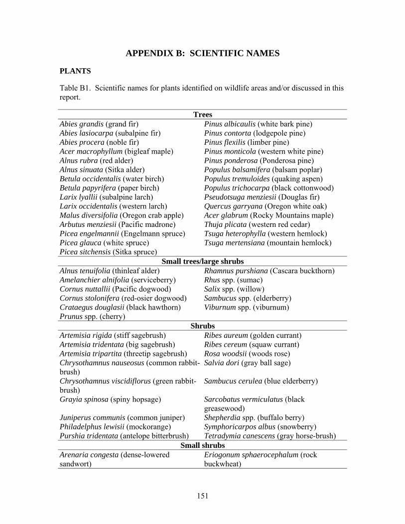
151
APPENDIX B: SCIENTIFIC NAMES
PLANTS
Table B1. Scientific names for plants identified on wildlife areas and/or discussed in this report.
Trees Abies grandis (grand fir) Pinus albicaulis (white bark pine) Abies lasiocarpa (subalpine fir) Pinus contorta (lodgepole pine) Abies procera (noble fir) Pinus flexilis (limber pine) Acer macrophyllum (bigleaf maple) Pinus monticola (western white pine) Alnus rubra (red alder) Pinus ponderosa (Ponderosa pine) Alnus sinuata (Sitka alder) Populus balsamifera (balsam poplar) Betula occidentalis (water birch) Populus tremuloides (quaking aspen) Betula papyrifera (paper birch) Populus trichocarpa (black cottonwood) Larix lyallii (subalpine larch) Pseudotsuga menziesii (Douglas fir) Larix occidentalis (western larch) Quercus garryana (Oregon white oak) Malus diversifolia (Oregon crab apple) Acer glabrum (Rocky Mountains maple) Arbutus menziesii (Pacific madrone) Thuja plicata (western red cedar) Picea engelmannii (Engelmann spruce) Tsuga heterophylla (western hemlock) Picea glauca (white spruce) Tsuga mertensiana (mountain hemlock) Picea sitchensis (Sitka spruce)
Small trees/large shrubs Alnus tenuifolia (thinleaf alder) Rhamnus purshiana (Cascara buckthorn) Amelanchier alnifolia (serviceberry) Rhus spp. (sumac) Cornus nuttallii (Pacific dogwood) Salix spp. (willow) Cornus stolonifera (red-osier dogwood) Sambucus spp. (elderberry) Crataegus douglasii (black hawthorn) Viburnum spp. (viburnum) Prunus spp. (cherry)
Shrubs Artemisia rigida (stiff sagebrush) Ribes aureum (golden currant) Artemisia tridentata (big sagebrush) Ribes cereum (squaw currant) Artemisia tripartita (threetip sagebrush) Rosa woodsii (woods rose) Chrysothamnus nauseosus (common rabbit-brush)
Salvia dori (gray ball sage)
Chrysothamnus viscidiflorus (green rabbit-brush)
Sambucus cerulea (blue elderberry)
Grayia spinosa (spiny hopsage) Sarcobatus vermiculatus (black greasewood)
Juniperus communis (common juniper) Shepherdia spp. (buffalo berry) Philadelphus lewisii (mockorange) Symphoricarpos albus (snowberry) Purshia tridentata (antelope bitterbrush) Tetradymia canescens (gray horse-brush)
Small shrubs Arenaria congesta (dense-lowered sandwort)
Eriogonum sphaerocephalum (rock buckwheat)

152
Arenaria franklinii (Franklin’s sandwort) Eriogonum strictum (strict buckwheat) Erigeron linearis (desert yellow daisy) Eriogonum thymoides (thyme-leaf
buckwheat) Eriogonum compositum (northern buckwheat)
Eurotia lanata (winterfat)
Eriogonum douglasii (Douglas’ buckwheat) Haplopappus stenophyllus (narrow-leaf goldenweed)
Eriogonum heracleoides (parsnip-flowered buckwheat)
Leptodactylon pungens (leptodactylon)
Eriogonum microthecum (slenderbush buckwheat)
Phlox hoodii (Hood’s phlox)
Eriogonum niveum (snow buckwheat) Phlox longifolia Grasses
Agropyron cristatum Poa bulbosa Agropyron intermedium Poa cusickii Bromus commutatus Poa pratensis Bromus tectorum Poa secunda Calamagrostis rubescens Pseudoreogneria spicata Carex douglasii Sitanion hystrix Carex filifolia Stipa comata Distichlis stricta Stipa occidentalis Elymus cinereus Stipa thurberiana Festuca idahoensis Taeniatherum caput-medusae Koeleria cristata Vulpia bromoides Oryzopsis hymenoides Vulpia microstachys Poa ampla Vulpia octoflora
Forbs Achillea millefolium Lepidium perfoliatum Acroptilon repens Lewisia rediviva Agoseris heterophylla Linaria dalmatica Amsinckia lycopsoides Linum perenne Antennaria dimorpha Lithophragma glabrum Arabis cusickii Lithospermum ruderale Arabis glabra Lomatium ambiguum Arabis holboellii Lomatium canbyi Astragalus lentiginosus Lomatium dissectum Astragalus purshii Lomatium geyeri Astragalus reventiformis Lomatium gormanii Astragalus spaldingii Lomatium grayi Astragalus speirocarpus Lomatium macrocarpum Balsamorhiza careyana Lomatium triternatum Balsamorhiza hookeri Lupinus lepidus Balsamorhiza sagittata Lupinus leucophyllus Brodiaea douglasii Lupinus sericeus Calochortus macrocarpus Lupinus sulphureus Castilleja thompsonii Lupinus wyethii

153
Centaurea diffusa Machaeranthera canescens Centaurea maculosa Medicago sativa Ceratocephala testiculata Mertensia longiflora Chaenactis douglasii Mertensia oblongifolia Chorispora tenella Microseris troximoides Cirsium undulatum Oenothera andina Cirsium vulgare Oenothera pallida Clematis ligusticifolia Opuntia polyacantha Collinsia grandiflora Orthocarpus tenuifolius Collinsia parviflora Pectocarya linearis Collomia linearis Penstemon gairdneri Commandra umbellata Perideridia gairdneri Conyza canadensis Phacelia hastata Crepis acuminata Phacelia linearis Crepis atribarba Phlox caespitosa Crocidium multicaule Phoenicaulis cheiranthoides Cymopterus terebinthinus Plantago patagonica Cynoglossum officinale Plectritis macrocera Delphinium nutallianum Polemonium micranthum Descurainia pinnata Polygonum aviculare Dodecatheon conjugens Ranunculus glaberrimus Draba verna Salsola kali Epilobium brachycarpum Saxifraga occidentalis Epilobium minutum Sedum lanceolatum Erigeron corymbosus Senecio intergerrimus Erigeron filifolius Silene douglasii Erigeron poliospermus Sisymbrium altissimum Erigeron pumilis Sphaeralcea munroana Eriogonum elatum Taraxacum officinale Erodium cicutarium Townsendia florifera Fritillaria pudica Tragopogon dubius Heuchera cylindrica Trifolium macrocephalum Holosteum umbellatum Verbascum thapsus Hydrophyllum capitatum Viola trinervata Lactuca serriola Zigadenus paniculatus Lepidium latifolium
MAMMALS
Table B2. Scientific names for mammals identified on wildlife areas and/or discussed in this report.
Common name Scientific name Beaver Castor canadensis Badger Taxidea taxus Bighorn sheep Ovis canadensis Black-tailed jackrabbit Lepus californicus
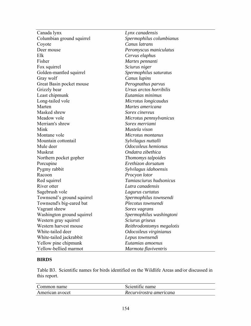
154
Canada lynx Lynx canadensis Columbian ground squirrel Spermophilus columbianus Coyote Canus latrans Deer mouse Peromyscus maniculatus Elk Cervus elaphus Fisher Martes pennanti Fox squirrel Sciurus niger Golden-mantled squirrel Spermophilus saturatus Gray wolf Canus lupins Great Basin pocket mouse Perognathus parvus Grizzly bear Ursus arctos horribilis Least chipmunk Eutamias minimus Long-tailed vole Microtus longicaudus Marten Martes americana Masked shrew Sorex cinereus Meadow vole Microtus pennsylvanicus Merriam's shrew Sorex merriami Mink Mustela vison Montane vole Microtus montanus Mountain cottontail Sylvilagus nuttalli Mule deer Odocoileus hemionus Muskrat Ondatra zibethica Northern pocket gopher Thomomys talpoides Porcupine Erethizon dorsatum Pygmy rabbit Sylvilagus idahoensis Racoon Procyon lotor Red squirrel Tamiasciurus hudsonicus River otter Lutra canadensis Sagebrush vole Lagurus curtatus Townsend’s ground squirrel Spermophilus townsendi Townsend's big-eared bat Plecotus townsendi Vagrant shrew Sorex vagrans Washington ground squirrel Spermophilus washingtoni Western gray squirrel Sciurus griseus Western harvest mouse Reithrodontomys megalotis White-tailed deer Odocoileus virginianus White-tailed jackrabbit Lepus townsendi Yellow pine chipmunk Eutamias amoenus Yellow-bellied marmot Marmota flaviventris
BIRDS
Table B3. Scientific names for birds identified on the Wildlife Areas and/or discussed in this report.
Common name Scientific name American avocet Recurvirostra americana
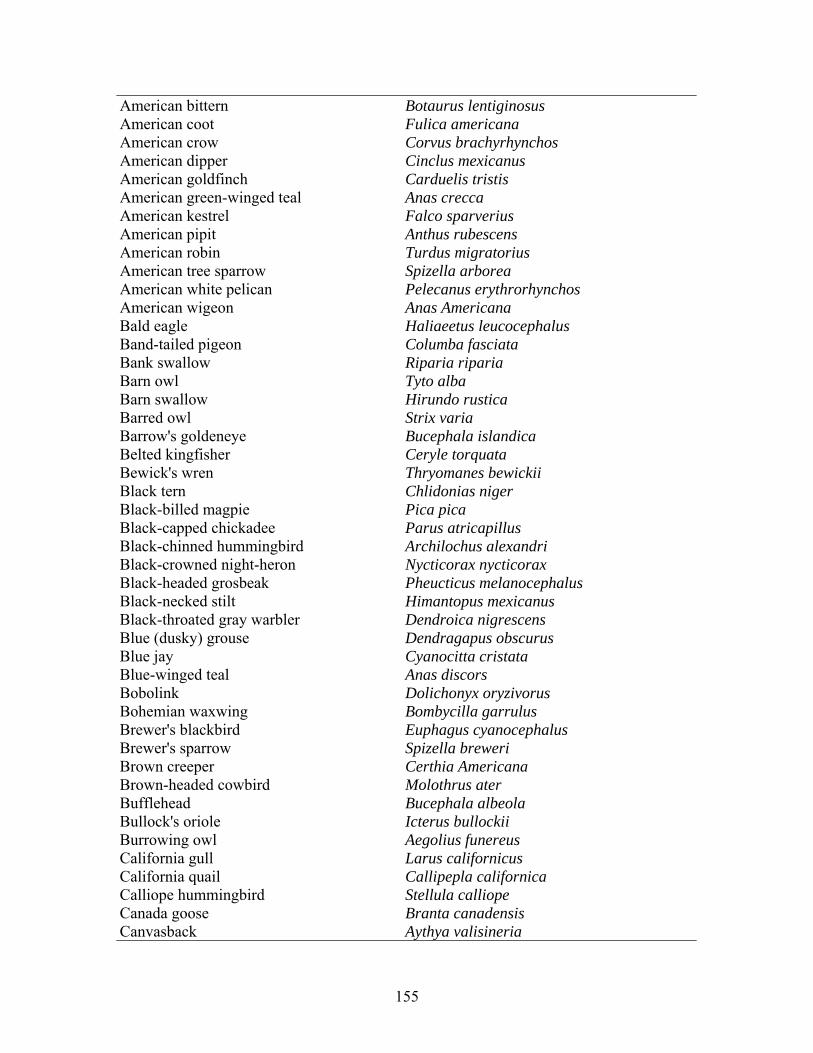
155
American bittern Botaurus lentiginosus American coot Fulica americana American crow Corvus brachyrhynchos American dipper Cinclus mexicanus American goldfinch Carduelis tristis American green-winged teal Anas crecca American kestrel Falco sparverius American pipit Anthus rubescens American robin Turdus migratorius American tree sparrow Spizella arborea American white pelican Pelecanus erythrorhynchos American wigeon Anas Americana Bald eagle Haliaeetus leucocephalus Band-tailed pigeon Columba fasciata Bank swallow Riparia riparia Barn owl Tyto alba Barn swallow Hirundo rustica Barred owl Strix varia Barrow's goldeneye Bucephala islandica Belted kingfisher Ceryle torquata Bewick's wren Thryomanes bewickii Black tern Chlidonias niger Black-billed magpie Pica pica Black-capped chickadee Parus atricapillus Black-chinned hummingbird Archilochus alexandri Black-crowned night-heron Nycticorax nycticorax Black-headed grosbeak Pheucticus melanocephalus Black-necked stilt Himantopus mexicanus Black-throated gray warbler Dendroica nigrescens Blue (dusky) grouse Dendragapus obscurus Blue jay Cyanocitta cristata Blue-winged teal Anas discors Bobolink Dolichonyx oryzivorus Bohemian waxwing Bombycilla garrulus Brewer's blackbird Euphagus cyanocephalus Brewer's sparrow Spizella breweri Brown creeper Certhia Americana Brown-headed cowbird Molothrus ater Bufflehead Bucephala albeola Bullock's oriole Icterus bullockii Burrowing owl Aegolius funereus California gull Larus californicus California quail Callipepla californica Calliope hummingbird Stellula calliope Canada goose Branta canadensis Canvasback Aythya valisineria
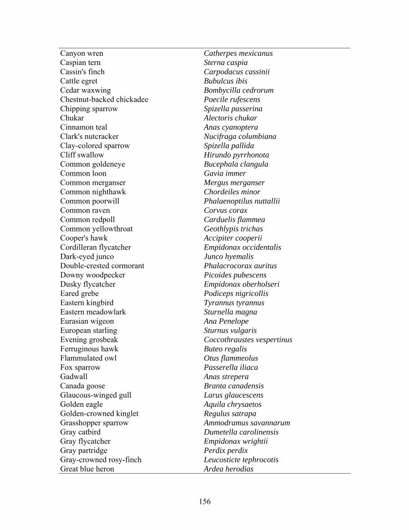
156
Canyon wren Catherpes mexicanus Caspian tern Sterna caspia Cassin's finch Carpodacus cassinii Cattle egret Bubulcus ibis Cedar waxwing Bombycilla cedrorum Chestnut-backed chickadee Poecile rufescens Chipping sparrow Spizella passerina Chukar Alectoris chukar Cinnamon teal Anas cyanoptera Clark's nutcracker Nucifraga columbiana Clay-colored sparrow Spizella pallida Cliff swallow Hirundo pyrrhonota Common goldeneye Bucephala clangula Common loon Gavia immer Common merganser Mergus merganser Common nighthawk Chordeiles minor Common poorwill Phalaenoptilus nuttallii Common raven Corvus corax Common redpoll Carduelis flammea Common yellowthroat Geothlypis trichas Cooper's hawk Accipiter cooperii Cordilleran flycatcher Empidonax occidentalis Dark-eyed junco Junco hyemalis Double-crested cormorant Phalacrocorax auritus Downy woodpecker Picoides pubescens Dusky flycatcher Empidonax oberholseri Eared grebe Podiceps nigricollis Eastern kingbird Tyrannus tyrannus Eastern meadowlark Sturnella magna Eurasian wigeon Ana Penelope European starling Sturnus vulgaris Evening grosbeak Coccothraustes vespertinus Ferruginous hawk Buteo regalis Flammulated owl Otus flammeolus Fox sparrow Passerella iliaca Gadwall Anas strepera Canada goose Branta canadensis Glaucous-winged gull Larus glaucescens Golden eagle Aquila chrysaetos Golden-crowned kinglet Regulus satrapa Grasshopper sparrow Ammodramus savannarum Gray catbird Dumetella carolinensis Gray flycatcher Empidonax wrightii Gray partridge Perdix perdix Gray-crowned rosy-finch Leucosticte tephrocotis Great blue heron Ardea herodias
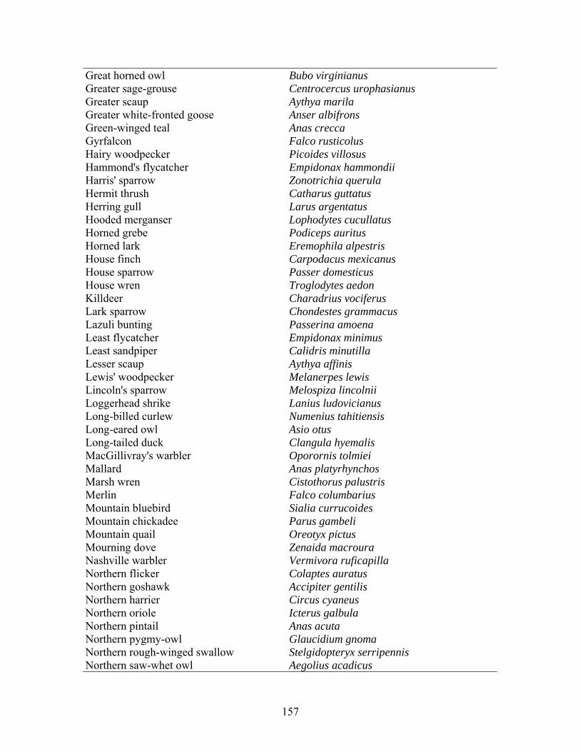
157
Great horned owl Bubo virginianus Greater sage-grouse Centrocercus urophasianus Greater scaup Aythya marila Greater white-fronted goose Anser albifrons Green-winged teal Anas crecca Gyrfalcon Falco rusticolus Hairy woodpecker Picoides villosus Hammond's flycatcher Empidonax hammondii Harris' sparrow Zonotrichia querula Hermit thrush Catharus guttatus Herring gull Larus argentatus Hooded merganser Lophodytes cucullatus Horned grebe Podiceps auritus Horned lark Eremophila alpestris House finch Carpodacus mexicanus House sparrow Passer domesticus House wren Troglodytes aedon Killdeer Charadrius vociferus Lark sparrow Chondestes grammacus Lazuli bunting Passerina amoena Least flycatcher Empidonax minimus Least sandpiper Calidris minutilla Lesser scaup Aythya affinis Lewis' woodpecker Melanerpes lewis Lincoln's sparrow Melospiza lincolnii Loggerhead shrike Lanius ludovicianus Long-billed curlew Numenius tahitiensis Long-eared owl Asio otus Long-tailed duck Clangula hyemalis MacGillivray's warbler Oporornis tolmiei Mallard Anas platyrhynchos Marsh wren Cistothorus palustris Merlin Falco columbarius Mountain bluebird Sialia currucoides Mountain chickadee Parus gambeli Mountain quail Oreotyx pictus Mourning dove Zenaida macroura Nashville warbler Vermivora ruficapilla Northern flicker Colaptes auratus Northern goshawk Accipiter gentilis Northern harrier Circus cyaneus Northern oriole Icterus galbula Northern pintail Anas acuta Northern pygmy-owl Glaucidium gnoma Northern rough-winged swallow Stelgidopteryx serripennis Northern saw-whet owl Aegolius acadicus
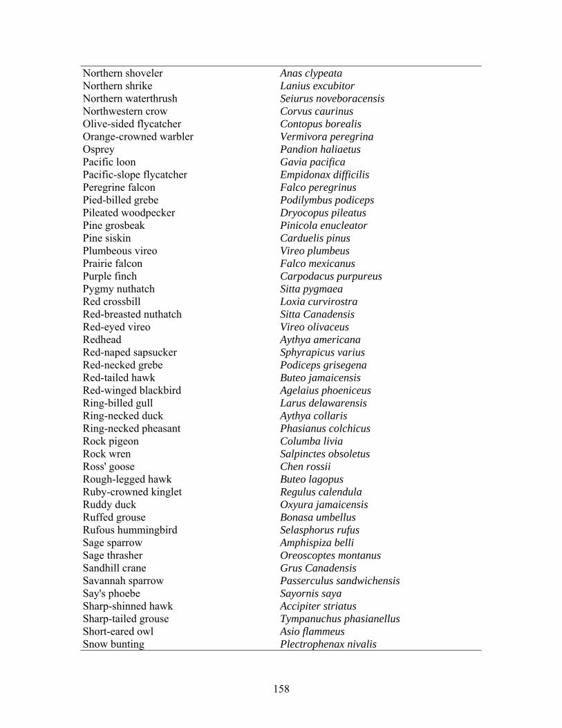
158
Northern shoveler Anas clypeata Northern shrike Lanius excubitor Northern waterthrush Seiurus noveboracensis Northwestern crow Corvus caurinus Olive-sided flycatcher Contopus borealis Orange-crowned warbler Vermivora peregrina Osprey Pandion haliaetus Pacific loon Gavia pacifica Pacific-slope flycatcher Empidonax difficilis Peregrine falcon Falco peregrinus Pied-billed grebe Podilymbus podiceps Pileated woodpecker Dryocopus pileatus Pine grosbeak Pinicola enucleator Pine siskin Carduelis pinus Plumbeous vireo Vireo plumbeus Prairie falcon Falco mexicanus Purple finch Carpodacus purpureus Pygmy nuthatch Sitta pygmaea Red crossbill Loxia curvirostra Red-breasted nuthatch Sitta Canadensis Red-eyed vireo Vireo olivaceus Redhead Aythya americana Red-naped sapsucker Sphyrapicus varius Red-necked grebe Podiceps grisegena Red-tailed hawk Buteo jamaicensis Red-winged blackbird Agelaius phoeniceus Ring-billed gull Larus delawarensis Ring-necked duck Aythya collaris Ring-necked pheasant Phasianus colchicus Rock pigeon Columba livia Rock wren Salpinctes obsoletus Ross' goose Chen rossii Rough-legged hawk Buteo lagopus Ruby-crowned kinglet Regulus calendula Ruddy duck Oxyura jamaicensis Ruffed grouse Bonasa umbellus Rufous hummingbird Selasphorus rufus Sage sparrow Amphispiza belli Sage thrasher Oreoscoptes montanus Sandhill crane Grus Canadensis Savannah sparrow Passerculus sandwichensis Say's phoebe Sayornis saya Sharp-shinned hawk Accipiter striatus Sharp-tailed grouse Tympanuchus phasianellus Short-eared owl Asio flammeus Snow bunting Plectrophenax nivalis

159
Snow goose Chen caerulescens Solitary vireo Vireo solitarius Song sparrow Melospiza melodia Sora Porzana carolina Spotted owl Strix occidentalis Spotted sandpiper Actitis macularia Spotted towhee Pipilo erythrophthalmus Steller's jay Cyanocitta stelleri Surf scoter Melanitta perspicillata Swainson's hawk Buteo swainsoni Swainson's thrush Catharus ustulatus Thayer's gull Larus thayeri Townsend's solitaire Myadestes townsendi Townsend's warbler Dendroica townsendi Tree swallow Tachycineta bicolor Trumpeter swan Cygnus buccinator Tundra swan Cygnus columbianus Turkey vulture Cathartes aura Varied thrush Ixoreus naevius Vaux's swift Chaetura vauxi Veery Catharus fuscescens Vesper sparrow Pooecetes gramineus Violet-green swallow Tachycineta thalassina Virginia rail Rallus limicola Warbling vireo Vireo gilvus Western bluebird Sialia mexicana Western grebe Aechmophorus occidentalis Western gull Larus occidentalis Western kingbird Tyrannus verticalis Western meadowlark Sturnella neglecta Western tanager Piranga ludoviciana Western wood-pewee Contopus sordidulus White-breasted nuthatch Sitta carolinensis White-crowned sparrow Zonotrichia leucophrys White-headed woodpecker Picoides albolarvatus White-throated sparrow Zonotrichia albicollis White-throated swift Aeronautes saxatalis White-winged scoter Melanitta fusca Wild turkey Meleagris gallopavo Williamson’s sapsucker Sphyrapicus thyroideus Willow flycatcher Empidonax traillii Wilson's phalarope Phalaropus tricolor Wilson's snipe Gallinago gallinago Wilson's warbler Wilsonia pusilla Winter wren Troglodytes troglodytes Wood duck Aix sponsa
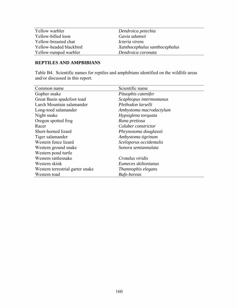
160
Yellow warbler Dendroica petechia Yellow-billed loon Gavia adamsii Yellow-breasted chat Icteria virens Yellow-headed blackbird Xanthocephalus xanthocephalus Yellow-rumped warbler Dendroica coronata
REPTILES AND AMPBIBIANS
Table B4. Scientific names for reptiles and amphibians identified on the wildlife areas and/or discussed in this report.
Common name Scientific name Gopher snake Pituophis catenifer Great Basin spadefoot toad Scaphiopus intermontanus Larch Mountain salamander Plethodon larselli Long-toed salamander Ambystoma macrodactylum Night snake Hypsiglena torquata Oregon spotted frog Rana pretiosa Racer Coluber constrictor Short-horned lizard Phrynosoma douglassii Tiger salamander Ambystoma tigrinum Western fence lizard Sceloporus occidentalis Western ground snake Sonora semiannulata Western pond turtle Western rattlesnake Crotalus viridis Western skink Eumeces skiltonianus Western terrestrial garter snake Thamnophis elegans Western toad Bufo boreas

161
APPENDIX C: SAMPLE DATA FORMS

162

163

164