Embed Size (px)
Citation preview
Introduction
This chapter gives example questions based on the text, together with example
answers. The purpose is to allow students opportunity to gain greater insight and
experience in applying their understanding. Some questions seek numerical
answers while others provide opportunity to express opinions. In the latter case,
example opinions are given in the answers, but these are not necessarily unique
and students are encouraged to propose alternative or additional opinions and to
discuss these with their instructor. In these questions the time within a day is given
in local time expressed in military-time format, i.e., 6:00 AM is written as 06:00
and 3:15 PM as 15:15.
Example questions
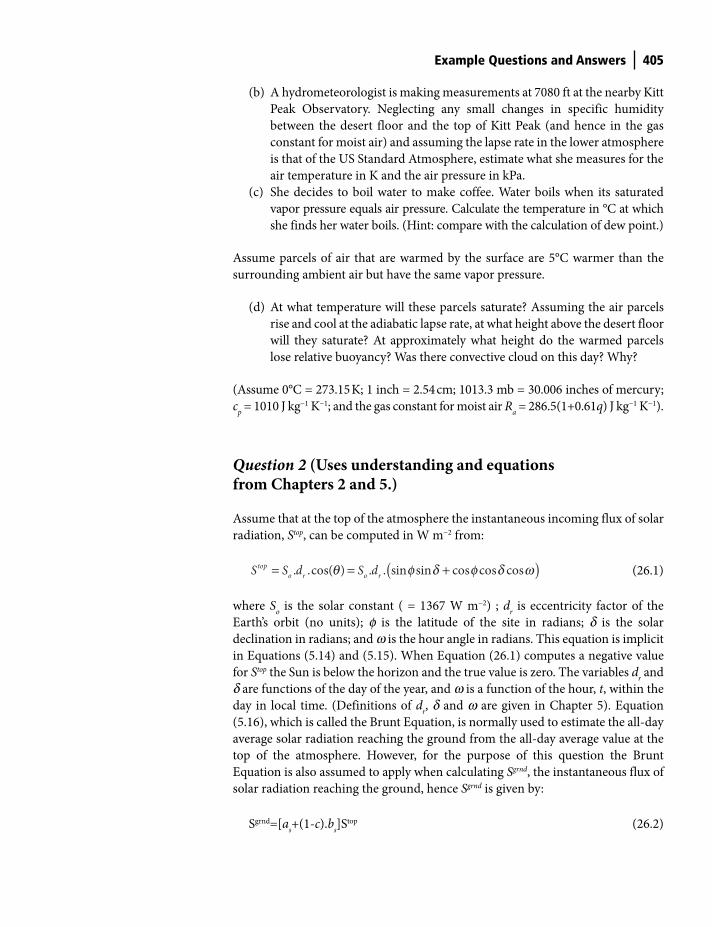
Question 1 (Uses understanding and equations from Chapters 2 and 3.)
At 14:00 on June 25 just above the ground near the desert floor about 60 miles west
of Tucson, at an altitude of 3700 ft, the temperature and pressure of the air are
114°F and 29.8 inches (of mercury), respectively, and the relative humidity is 25%.
(a) What are the air temperature in °C and K, the air pressure in mb and in
kPa, the saturated vapor pressure at air temperature in kPa, the vapor
pressure in kPa, the specific humidity in kg kg−1 and Ra, the gas constant,
for the moist air in J kg−1 K?
26 Example Questions and Answers
Terrestrial Hydrometeorology, First Edition. W. James Shuttleworth.
© 2012 John Wiley & Sons, Ltd. Published 2012 by John Wiley & Sons, Ltd.
Shuttleworth_c26.indd 404Shuttleworth_c26.indd 404 11/3/2011 6:37:21 PM11/3/2011 6:37:21 PM
Example Questions and Answers 405
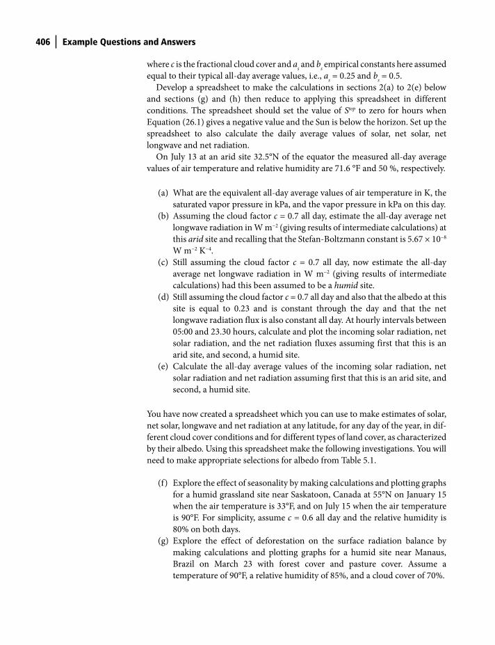
(b) A hydrometeorologist is making measurements at 7080 ft at the nearby Kitt
Peak Observatory. Neglecting any small changes in specific humidity
between the desert floor and the top of Kitt Peak (and hence in the gas
constant for moist air) and assuming the lapse rate in the lower atmosphere
is that of the US Standard Atmosphere, estimate what she measures for the
air temperature in K and the air pressure in kPa.
(c) She decides to boil water to make coffee. Water boils when its saturated
vapor pressure equals air pressure. Calculate the temperature in °C at which
she finds her water boils. (Hint: compare with the calculation of dew point.)
Assume parcels of air that are warmed by the surface are 5°C warmer than the
surrounding ambient air but have the same vapor pressure.
(d) At what temperature will these parcels saturate? Assuming the air parcels
rise and cool at the adiabatic lapse rate, at what height above the desert floor
will they saturate? At approximately what height do the warmed parcels
lose relative buoyancy? Was there convective cloud on this day? Why?
(Assume 0°C = 273.15 K; 1 inch = 2.54 cm; 1013.3 mb = 30.006 inches of mercury;
cp = 1010 J kg−1 K−1; and the gas constant for moist air R
a = 286.5(1+0.61q) J kg−1 K−1).
Question 2 (Uses understanding and equations from Chapters 2 and 5.)
Assume that at the top of the atmosphere the instantaneous incoming flux of solar
radiation, Stop, can be computed in W m−2 from:
( ). .cos( ) . . sin sin cos cos costopo r o rS S d S d= = +q f d f d w (26.1)
where So is the solar constant ( = 1367 W m−2) ; d
r is eccentricity factor of the
Earth’s orbit (no units); f is the latitude of the site in radians; d is the solar
declination in radians; and w is the hour angle in radians. This equation is implicit
in Equations (5.14) and (5.15). When Equation (26.1) computes a negative value
for Stop the Sun is below the horizon and the true value is zero. The variables dr and
d are functions of the day of the year, and w is a function of the hour, t, within the
day in local time. (Definitions of dr, d and w are given in Chapter 5). Equation
(5.16), which is called the Brunt Equation, is normally used to estimate the all-day
average solar radiation reaching the ground from the all-day average value at the
top of the atmosphere. However, for the purpose of this question the Brunt
Equation is also assumed to apply when calculating Sgrnd, the instantaneous flux of
solar radiation reaching the ground, hence Sgrnd is given by:
Sgrnd=[as+(1-c).b
s]Stop (26.2)
Shuttleworth_c26.indd 405Shuttleworth_c26.indd 405 11/3/2011 6:37:22 PM11/3/2011 6:37:22 PM
406 Example Questions and Answers
where c is the fractional cloud cover and as and b
s empirical constants here assumed
equal to their typical all-day average values, i.e., as = 0.25 and b
s = 0.5.
Develop a spreadsheet to make the calculations in sections 2(a) to 2(e) below
and sections (g) and (h) then reduce to applying this spreadsheet in different
conditions. The spreadsheet should set the value of Stop to zero for hours when
Equation (26.1) gives a negative value and the Sun is below the horizon. Set up the
spreadsheet to also calculate the daily average values of solar, net solar, net
longwave and net radiation.
On July 13 at an arid site 32.5°N of the equator the measured all-day average
values of air temperature and relative humidity are 71.6 °F and 50 %, respectively.
(a) What are the equivalent all-day average values of air temperature in K, the
saturated vapor pressure in kPa, and the vapor pressure in kPa on this day.
(b) Assuming the cloud factor c = 0.7 all day, estimate the all-day average net
longwave radiation in W m−2 (giving results of intermediate calculations) at
this arid site and recalling that the Stefan-Boltzmann constant is 5.67 × 10⁻⁸
W m−2 K−4.
(c) Still assuming the cloud factor c = 0.7 all day, now estimate the all-day
average net longwave radiation in W m−2 (giving results of intermediate
calculations) had this been assumed to be a humid site.
(d) Still assuming the cloud factor c = 0.7 all day and also that the albedo at this
site is equal to 0.23 and is constant through the day and that the net
longwave radiation flux is also constant all day. At hourly intervals between
05:00 and 23.30 hours, calculate and plot the incoming solar radiation, net
solar radiation, and the net radiation fluxes assuming first that this is an
arid site, and second, a humid site.
(e) Calculate the all-day average values of the incoming solar radiation, net
solar radiation and net radiation assuming first that this is an arid site, and
second, a humid site.
You have now created a spreadsheet which you can use to make estimates of solar,
net solar, longwave and net radiation at any latitude, for any day of the year, in dif-
ferent cloud cover conditions and for different types of land cover, as characterized
by their albedo. Using this spreadsheet make the following investigations. You will
need to make appropriate selections for albedo from Table 5.1.
(f) Explore the effect of seasonality by making calculations and plotting graphs
for a humid grassland site near Saskatoon, Canada at 55°N on January 15
when the air temperature is 33°F, and on July 15 when the air temperature
is 90°F. For simplicity, assume c = 0.6 all day and the relative humidity is
80% on both days.
(g) Explore the effect of deforestation on the surface radiation balance by
making calculations and plotting graphs for a humid site near Manaus,
Brazil on March 23 with forest cover and pasture cover. Assume a
temperature of 90°F, a relative humidity of 85%, and a cloud cover of 70%.
Shuttleworth_c26.indd 406Shuttleworth_c26.indd 406 11/3/2011 6:37:23 PM11/3/2011 6:37:23 PM
Example Questions and Answers 407
Question 3 (Uses understanding and equations from Chapters 1, 4, 6, and 7.)
A farmer has a copy of Terrestrial Hydrometeorology and therefore has
wide-ranging knowledge of the subject. He has a field that is currently bare soil
near Casa Grande, Arizona which is 32.5°N of the equator. This is the arid site for
which you calculated values of net radiation in 2(d). He recently irrigated the field
prior to planting and the sandy soil is close to saturated. He decides to measure the
evaporation loss from the field but he only has three thermometers and a set of tall
stepladders with which to do so. He installs one thermometer in the soil to measure
the temperature very close to the surface of the soil. He wraps the mercury bulb of
a second thermometer in a small piece of cloth that he is careful to keep moist so
that it measures wet bulb temperature. The third thermometer he uses as a dry
bulb thermometer to measure air temperature.
Starting at midnight on July 13 he measures the wet bulb and dry bulb
temperature 0.5 m above the ground and then quickly runs up the stepladder and
makes the same measurements at 3.0 m from the ground. Every 5 minutes he
repeats this operation throughout the next 24 hours. In his spare time he monitors
the thermometer in the soil and notices that the minimum temperature of 20°C
occurs at 01:00 and the maximum temperature of 24°C occurs at 13:00. He also
monitors the sky and decides that the fractional cloud cover is 0.7 and fairly
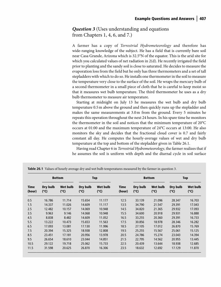
constant all day. He computes the hourly-average values of wet and dry bulb
temperature at the top and bottom of the stepladder given in Table 26.1.
Having read Chapter 6 in Terrestrial Hydrometeorology, the farmer realizes that if
he assumes the soil is uniform with depth and the diurnal cycle in soil surface
Table 26.1 Values of hourly average dry and wet bulb temperatures measured by the farmer in question 3.
Bottom Top Bottom Top
Time (hour)
Dry bulb (°C)
Wet bulb (°C)
Dry bulb (°C)
Wet bulb (°C)
Time (hour)
Dry bulb (°C)
Wet bulb (°C)
Dry bulb (°C)
Wet bulb (°C)
0.5 16.786 11.714 15.654 11.177 12.5 33.139 21.096 28.347 16.7031.5 14.337 11.026 14.609 11.117 13.5 34.790 21.547 29.391 17.0432.5 12.482 10.157 14.069 10.948 14.5 34.820 21.365 29.932 17.0933.5 9.963 9.146 14.068 10.948 15.5 34.600 20.918 29.931 16.8884.5 8.838 8.482 14.609 11.052 16.5 33.255 20.360 29.391 16.7335.5 13.222 10.473 15.653 11.563 17.5 30.856 18.978 28.346 16.2826.5 17.093 13.081 17.130 11.996 18.5 27.105 17.012 26.870 15.7697.5 20.394 15.325 18.938 12.808 19.5 25.255 15.567 25.061 15.1258.5 23.451 17.181 20.956 13.978 20.5 24.786 15.274 23.043 14.3949.5 26.654 18.610 23.044 14.851 21.5 22.795 14.562 20.955 13.44510.5 29.122 19.718 25.062 15.733 22.5 20.439 13.644 18.938 12.68511.5 31.598 20.625 26.870 16.306 23.5 18.632 12.692 17.129 11.870
Shuttleworth_c26.indd 407Shuttleworth_c26.indd 407 11/3/2011 6:37:23 PM11/3/2011 6:37:23 PM
408 Example Questions and Answers
temperature is sinusoidal, and if he chooses the form of the sinusoidal wave to agree
with the timing and magnitude of the minimum and maximum soil temperatures
that he measured and also selects values of soil properties appropriate for the moist
sandy soil, he can calculate the soil heat flux at any time during the day.
(a) What were the values of the mean soil surface temperature, and the
amplitude and the time slip of the cycle in soil surface temperature that he
selected?
(b) What were the values of soil thermal conductivity, ks, and thermal
diffusivity, αs, that he selected, what was the value of damping depth, D, for
the daily time period (expressed in seconds) that he calculated. Which
equation from Terrestrial Hydrometeorology did he use to calculate the
instantaneous surface soil heat flux?
The farmer assumes that the psychrometric constant is 0.0667 kPa K−1 when
applying the wet-bulb equation and when calculating the Bowen ratio. For
simplicity he also assumes that the difference in virtual potential temperature is
equal to the difference in measured air temperature between the two levels. (This
is a common assumption when calculating Bowen ratio). In the course of his
calculations he found that the all-day average air temperature and vapor pressure
at the bottom level were the same as those you calculated and used in question
2(a). Using these values with the day of the year and latitude of the site he was able
to calculate the same estimates of net radiation for this arid site that you calculated
in question 2(d). You can therefore adopt those values of hourly net radiation for
use in this question.
(c) Develop a spreadsheet to tabulate the values of vapor pressure at the bot-
tom level, vapor pressure at the top level, Bowen ratio, net radiation [copied
from 2(e)], soil heat flux, available energy, latent heat flux and sensible heat
flux at hourly intervals between 0.5 and 23.5 hours.
(d) Plot the calculated net radiation, soil heat flux, available energy, latent heat
flux and sensible heat flux as a function of time through the day.
(e) What were the all-day average values of the Bowen ratio and Evaporative
Fraction at his site on this day?
(f) Suppose the farmer had chosen to neglect soil heat flux in his calculation of
available energy. Without recalculating all the rates, can you suggest
whether he would have overestimated or underestimated the all-day
average evaporative fraction and explain why?
Question 4 (Uses understanding from Chapters 1, 2, and 8.)
(a) Shuttleworth says, ‘As an annual-average, the value is about 1.2 m. However
we, as land dwellers, see only about 10% of this, and we lose almost two-
thirds back to the atmosphere. We keep an even smaller proportion
Shuttleworth_c26.indd 408Shuttleworth_c26.indd 408 11/3/2011 6:37:23 PM11/3/2011 6:37:23 PM
Example Questions and Answers 409
in Arizona.’ In your opinion, what is Shuttleworth talking about? The
annual-average of what is about 1.2 m? How do we lose two-thirds back to
the atmosphere? Approximately what proportion do we keep in Arizona?
(b) Shuttleworth says, ‘These two components of these models have jargon
names and are run alternately. The first applies the conservation laws while
the second, by representing relevant processes, changes the divergence
terms in these laws prior to their next application.’ In your opinion, what
components of what models is he talking about and what are their jargon
names. Which ‘laws’ does he refer to? Can you suggest some of the relevant
processes that change the divergence terms in these laws?
(c) Shuttleworth says, ‘Of course, if all the continents were constrained to be in
the tropics then, as a global average, the proportion of the Sun’s radiant
energy reflected at the Earth’s surface would vary less between summer and
winter.’ In your opinion, what is at least one reason why Shuttleworth might
be correct?
(d) Shuttleworth says, ‘Most of the time the temperature gradient in the lower
atmosphere is less than the dry adiabatic lapse rate. Water vapor is also
strongly concentrated at the bottom of the atmosphere. Presumably, the
same processes are responsible for both of these phenomena.’ In your
opinion, could Shuttleworth’s presumption be correct? What process or
processes might simultaneously reduce the actual lapse rate below the
adiabatic rate and also reduce the vapor content of the atmosphere at levels
well above the ground?
(e) Shuttleworth says, ‘These models are used in three main ways, each with a
different objective. However, in fact, one application was a by-product of
the original model application. “Initiation” is a keyword in all of these
applications.’ In your opinion, now what is Shuttleworth talking about?
What models? What are the three different objectives? Can you suggest
why he puts emphasis on model initiation?
(f) Shuttleworth says, ‘The specific heat is 4 times bigger and the density is
nearly 1000 times bigger. If this wasn’t true, we might have http://www.
weather.gov/ but we probably would not have http://www.cpc.ncep.noaa.
gov/’ In your opinion, what has a specific heat and density respectively 4
and 1000 times bigger than what? If this were not the case, can you explain
why in your opinion this might mean that http://www.cpc.ncep.noaa.gov/
would not be needed but http://www.weather.gov/ likely still would be?
(g) Shuttleworth says, ‘One important potential consequence of ‘greenhouse
warming’ is that it will enhance the hydrological cycle. It is interesting that
non-linearity in the basic relationship that would cause this enhancement
tends to compensate for the projected warming being twice as large at the
poles than at the equator.’ In your opinion, what does Shuttleworth mean
by this? Can you suggest what basic relationship might allow greenhouse
warming to enhance the hydrological cycle? Why might this relationship
be more effective at the equator, thus compensating for the potentially
enhanced warming at the poles?
Shuttleworth_c26.indd 409Shuttleworth_c26.indd 409 11/3/2011 6:37:23 PM11/3/2011 6:37:23 PM
410 Example Questions and Answers
Question 5 (Uses understanding from Chapter 9.)
The planet Malleable is fascinating. In many respects it is identical to the Earth. It
has identical dimensions and is located in a solar system identical to ours. It rotates
around an identical sun, in an identical orbit, and its solar declination changes
seasonally as does the Earth’s. Moreover, on average, the relative area of oceans and
continents is the same as that on Earth. The planet is the adopted home to an
advanced civilization that can manipulate the location of the continents on
Malleable’s surface. When it was settled, the ‘Founding Fathers’ of Malleable chose
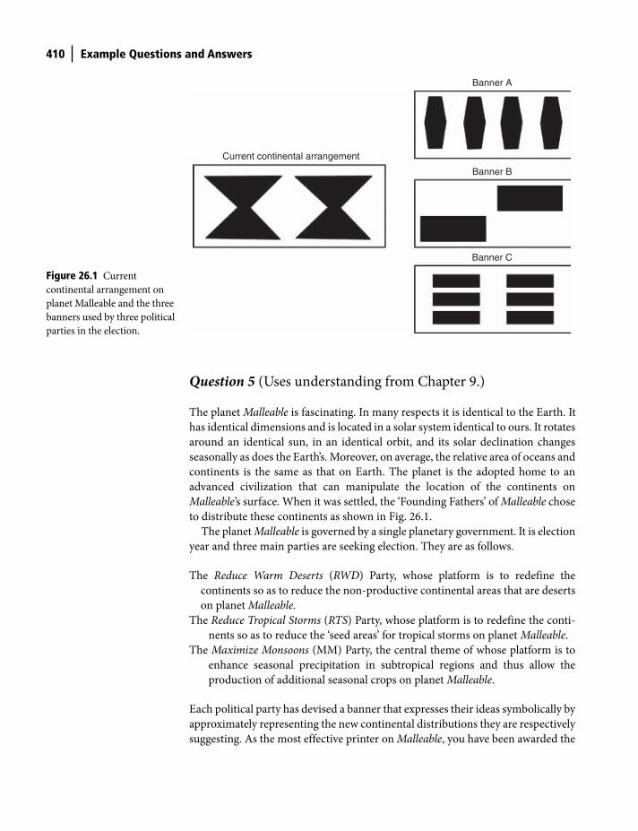
to distribute these continents as shown in Fig. 26.1.
The planet Malleable is governed by a single planetary government. It is election
year and three main parties are seeking election. They are as follows.
The Reduce Warm Deserts (RWD) Party, whose platform is to redefine the
continents so as to reduce the non-productive continental areas that are deserts
on planet Malleable.
The Reduce Tropical Storms (RTS) Party, whose platform is to redefine the conti-
nents so as to reduce the ‘seed areas’ for tropical storms on planet Malleable.
The Maximize Monsoons (MM) Party, the central theme of whose platform is to
enhance seasonal precipitation in subtropical regions and thus allow the
production of additional seasonal crops on planet Malleable.
Each political party has devised a banner that expresses their ideas symbolically by
approximately representing the new continental distributions they are respectively
suggesting. As the most effective printer on Malleable, you have been awarded the
Current continental arrangement
Banner A
Banner B
Banner C
Figure 26.1 Current
continental arrangement on
planet Malleable and the three
banners used by three political
parties in the election.
Shuttleworth_c26.indd 410Shuttleworth_c26.indd 410 11/3/2011 6:37:23 PM11/3/2011 6:37:23 PM
Example Questions and Answers 411
contract to print these banners. Unfortunately the three party symbols have
arrived at your printing works without you knowing which symbol belongs to
which party. On the basis of your understanding derived from Terrestrial
Hydrometeorology, you must choose the most appropriate symbol for each party’s
banner. These symbols are also shown in Fig. 26.1.
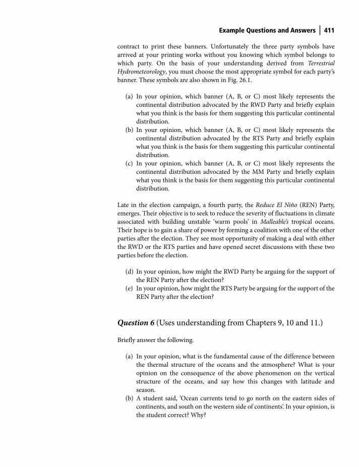
(a) In your opinion, which banner (A, B, or C) most likely represents the
continental distribution advocated by the RWD Party and briefly explain
what you think is the basis for them suggesting this particular continental
distribution.
(b) In your opinion, which banner (A, B, or C) most likely represents the
continental distribution advocated by the RTS Party and briefly explain
what you think is the basis for them suggesting this particular continental
distribution.
(c) In your opinion, which banner (A, B, or C) most likely represents the
continental distribution advocated by the MM Party and briefly explain
what you think is the basis for them suggesting this particular continental
distribution.
Late in the election campaign, a fourth party, the Reduce El Niño (REN) Party,
emerges. Their objective is to seek to reduce the severity of fluctuations in climate
associated with building unstable ‘warm pools’ in Malleable’s tropical oceans.
Their hope is to gain a share of power by forming a coalition with one of the other
parties after the election. They see most opportunity of making a deal with either
the RWD or the RTS parties and have opened secret discussions with these two
parties before the election.
(d) In your opinion, how might the RWD Party be arguing for the support of
the REN Party after the election?
(e) In your opinion, how might the RTS Party be arguing for the support of the
REN Party after the election?
Question 6 (Uses understanding from Chapters 9, 10 and 11.)
Briefly answer the following.
(a) In your opinion, what is the fundamental cause of the difference between
the thermal structure of the oceans and the atmosphere? What is your
opinion on the consequence of the above phenomenon on the vertical
structure of the oceans, and say how this changes with latitude and
season.
(b) A student said, ‘Ocean currents tend to go north on the eastern sides of
continents, and south on the western side of continents’. In your opinion, is
the student correct? Why?
Shuttleworth_c26.indd 411Shuttleworth_c26.indd 411 11/3/2011 6:37:23 PM11/3/2011 6:37:23 PM
412 Example Questions and Answers
(c) In your opinion, why do ocean currents tend to behave this way?
(d) Discuss the statement, ‘The geographical distribution of land masses
influences the effect of ocean circulation on tropical Sea Surface
Temperature’ in the context of the Atlantic Ocean, and give your opinion
on any consequences on the relative frequency of tropical storms in Cuba
and in northeast Brazil.
(e) A student said, ‘The hydroclimatic mechanism which most influences the
food supply of half the world’s population is related to difference in the way
surface radiation is shared for continents and oceans.’ In your opinion,
what did she mean?
(f) For clouds to occur in the atmosphere a mechanism which gives rising air
and therefore cooling air is required. In your opinion, what are two other
requirements and which of them is most likely to be the limiting
requirement?
(g) If a parcel of air is moister than its surroundings but it has the same
temperature and pressure, in your opinion will it tend to rise or will it tend
to fall? Briefly explain why.
(h) In convective conditions parcels of air are heated and start to rise because
they are warmer and lighter. As soon as a parcel rises the air cools. In your
opinion why does this cooling not necessarily stop the air parcel rising to
the cloud condensation level?
(i) Once the cloud condensation level is reached, cloud formation begins. Give
your opinion on what effect the condensation process will have on the
buoyancy of the parcel of air and its further ascent in the cloud.
(j) In a particular mid-latitude cloud, the air temperature is -25°C. In your
opinion, which phases of water (solid, liquid or vapor) are likely to be
present in the cloud, and what is likely to be the most important physical
mechanism giving ice particle growth in the cloud.
Question 7 (Uses understanding from Chapters 12, 13 and 14.)
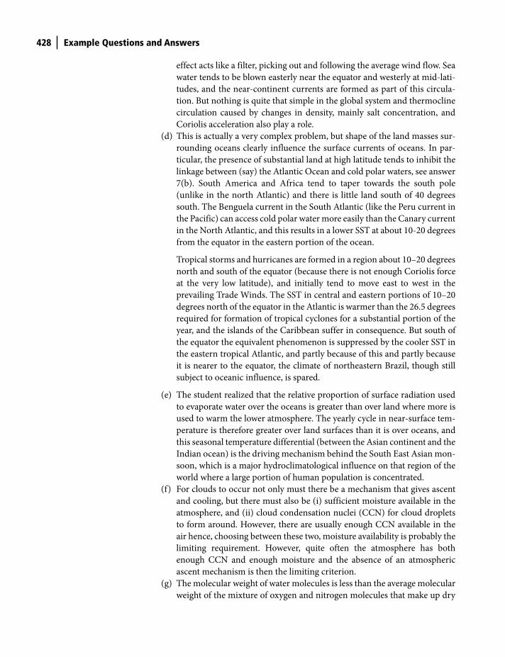
(a) Draw a diagram of what in your opinion is the ideal site and mounting for
a rain gauge. It should show its relation to surrounding objects and to the
ground. Give a brief explanation of why you consider your design to be
good. Discuss this design with your instructor.
(b) Obtain values of mean monthly precipitation for a site that interests you
(e.g., your home town, state, or country). Compute the Seasonality Index
from these data using the formulae given in your class notes (or an
alternative measure of seasonality if you prefer; there are alternative
measures.) Comment on what this index implies about the seasonality of
the precipitation climate that you choose.
(c) Using the same data you used in question 7(b), draw a ‘pie’ diagram to
illustrate the seasonal behavior of the rainfall showing the percentage
contributions to the annual rainfall in each month.
Shuttleworth_c26.indd 412Shuttleworth_c26.indd 412 11/3/2011 6:37:24 PM11/3/2011 6:37:24 PM
Example Questions and Answers 413
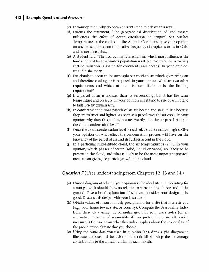
(d) During a storm the chart from a siphon rain gauge produced the (simu-
lated) form illustrated in Fig. 26.2. This was digitized to give the numerical
time sequence in Table 26.2. Plot the mass curve for this particular storm
and, on the basis of this mass curve, speculate as to whether the chart was
most likely to be for a frontal or convective storm and explain your
reasoning.
(e) The July rainfall amounts in Tanzania over the period 1931–1960 are given
in Table 13.1. Calculate the mean value and estimate the median value of
the July rainfall in Tanzania between 1931 and 1960. If you find they differ,
say why.
10
8
6
4
2
00 20 40 60
Time (minutes)
80 100 120
Rai
nfal
l (m
m)Figure 26.2 A (simulated) chart
of precipitation for a storm
measured using a siphon rain
gauge. Note that once the
chamber reaches a storage that is
equivalent to 10 mm of rainfall,
the chamber is siphoned empty
and then continues to refill as the
storm proceeds.
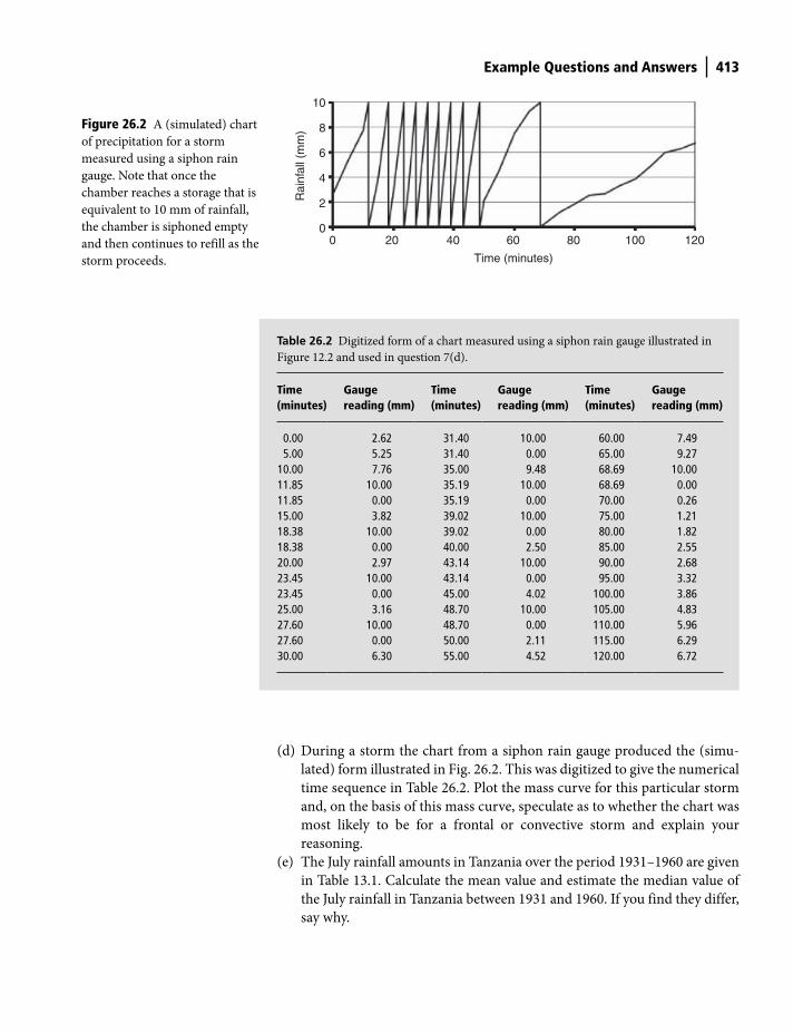
Table 26.2 Digitized form of a chart measured using a siphon rain gauge illustrated in
Figure 12.2 and used in question 7(d).
Time (minutes)
Gauge reading (mm)
Time (minutes)
Gauge reading (mm)
Time (minutes)
Gauge reading (mm)
0.00 2.62 31.40 10.00 60.00 7.495.00 5.25 31.40 0.00 65.00 9.27
10.00 7.76 35.00 9.48 68.69 10.0011.85 10.00 35.19 10.00 68.69 0.0011.85 0.00 35.19 0.00 70.00 0.2615.00 3.82 39.02 10.00 75.00 1.2118.38 10.00 39.02 0.00 80.00 1.8218.38 0.00 40.00 2.50 85.00 2.5520.00 2.97 43.14 10.00 90.00 2.6823.45 10.00 43.14 0.00 95.00 3.3223.45 0.00 45.00 4.02 100.00 3.8625.00 3.16 48.70 10.00 105.00 4.8327.60 10.00 48.70 0.00 110.00 5.9627.60 0.00 50.00 2.11 115.00 6.2930.00 6.30 55.00 4.52 120.00 6.72
Shuttleworth_c26.indd 413Shuttleworth_c26.indd 413 11/3/2011 6:37:24 PM11/3/2011 6:37:24 PM
414 Example Questions and Answers
(f) Compute and plot the time variations in the 7-year running mean for July
Tanzanian rainfall data between 1934 and 1957.
(g) Compute and plot the mass curve for July Tanzanian rainfall data between
1931 and 1960.
(h) Compute and plot the cumulative deviation for July Tanzanian rainfall data
between 1931 and 1960.
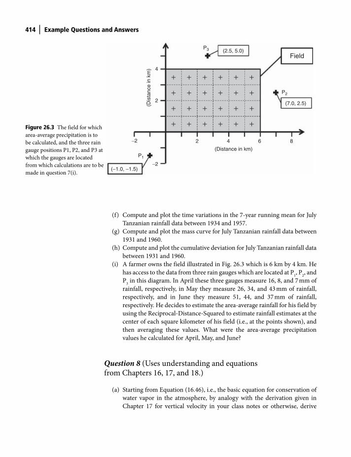
(i) A farmer owns the field illustrated in Fig. 26.3 which is 6 km by 4 km. He
has access to the data from three rain gauges which are located at P1, P
2, and
P3 in this diagram. In April these three gauges measure 16, 8, and 7 mm of
rainfall, respectively, in May they measure 26, 34, and 43 mm of rainfall,
respectively, and in June they measure 51, 44, and 37 mm of rainfall,
respectively. He decides to estimate the area-average rainfall for his field by
using the Reciprocal-Distance-Squared to estimate rainfall estimates at the
center of each square kilometer of his field (i.e., at the points shown), and
then averaging these values. What were the area-average precipitation
values he calculated for April, May, and June?
Question 8 (Uses understanding and equations from Chapters 16, 17, and 18.)
(a) Starting from Equation (16.46), i.e., the basic equation for conservation of
water vapor in the atmosphere, by analogy with the derivation given in
Chapter 17 for vertical velocity in your class notes or otherwise, derive
2−2
−2
4
4
(Distance in km)
6 8
2
P1
P2
P3
(−1.0, −1.5)
(2.5, 5.0)
(7.0, 2.5)
Field
+
+
+
+
+
+
+
+
+
+
+
+
+
+
+
+
+
+
+
+
+
+
+
+
(Dis
tanc
e in
km
)
Figure 26.3 The field for which
area-average precipitation is to
be calculated, and the three rain
gauge positions P1, P2, and P3 at
which the gauges are located
from which calculations are to be
made in question 7(i).
Shuttleworth_c26.indd 414Shuttleworth_c26.indd 414 11/3/2011 6:37:25 PM11/3/2011 6:37:25 PM
Example Questions and Answers 415
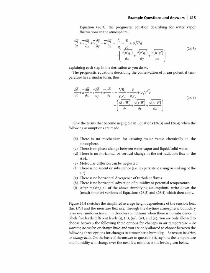
Equation (26.3), the prognostic equation describing for water vapor
fluctuations in the atmosphere:
( ) ( ) ( )
2
' ' ' ' ' '
a a
Sq q q q Eu v w qt x y z
u q v q w qx y z
∂ ∂ ∂ ∂+ + + = + + ∇
∂ ∂ ∂ ∂⎛ ⎞∂ ∂ ∂
− + +⎜ ⎟∂ ∂ ∂⎝ ⎠
ur r
(26.3)
explaining each step in the derivation as you do so.
The prognostic equations describing the conservation of mean potential tem-
perature has a similar form, thus:
( ) ( ) ( )
2
' ' ' ' ' '
n
a p a p
R Eu v wt x y z c c
u v wx y z
θ
∇∂θ ∂θ ∂θ ∂θ+ + + = − − + υ ∇ θ
∂ ∂ ∂ ∂⎛ ⎞∂ θ ∂ θ ∂ θ
− + +⎜ ⎟∂ ∂ ∂⎝ ⎠
r r
(26.4)
Give the terms that become negligible in Equations (26.3) and (26.4) when the
following assumptions are made.
(b) There is no mechanism for creating water vapor chemically in the
atmosphere.
(c) There is no phase change between water vapor and liquid/solid water.
(d) There is no horizontal or vertical change in the net radiation flux in the
ABL.
(e) Molecular diffusion can be neglected.
(f) There is no ascent or subsidence (i.e. no persistent rising or sinking of the
air).
(g) There is no horizontal divergence of turbulent fluxes.
(h) There is no horizontal advection of humidity or potential temperature.
(i) After making all of the above simplifying assumptions, write down the
(much simpler) versions of Equations (26.3) and (26.4) which then apply.
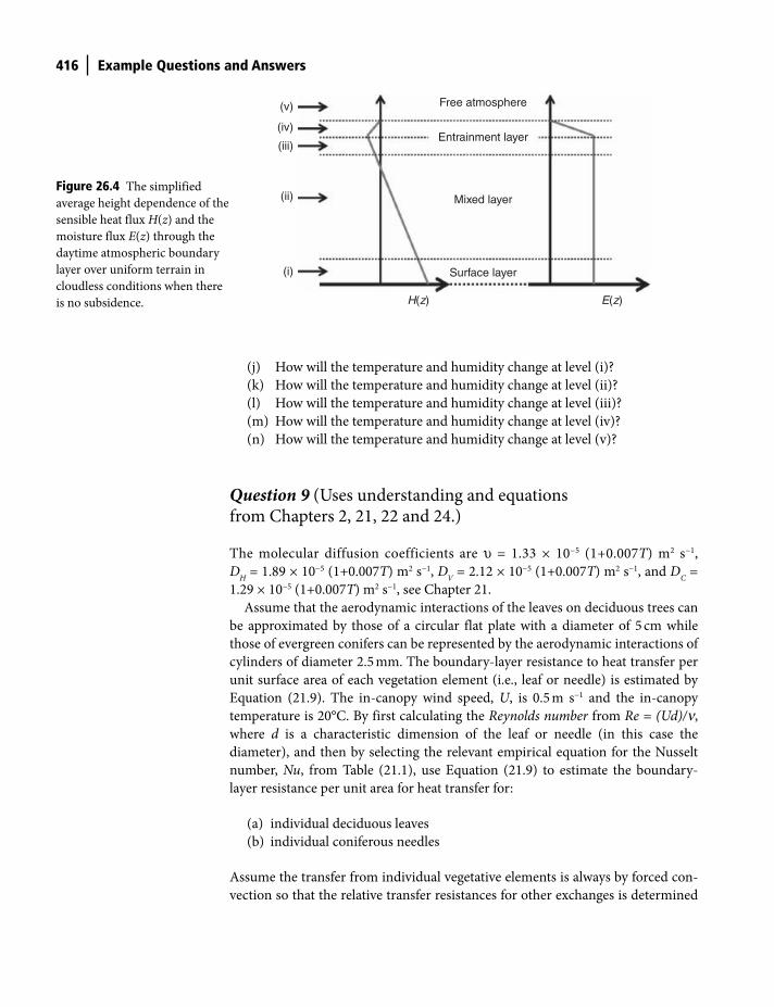
Figure 26.4 sketches the simplified average height dependence of the sensible heat
flux H(z) and the moisture flux E(z) through the daytime atmospheric boundary
layer over uniform terrain in cloudless conditions when there is no subsidence. It
labels five levels different levels (i), (ii), (iii), (iv), and (v). You are only allowed to
choose between the following three options for changes in air temperature – be
warmer, be cooler, or change little; and you are only allowed to choose between the
following three options for changes in atmospheric humidity – be wetter, be drier,
or change little. On the basis of the answer to question (i), say how the temperature
and humidity will change over the next few minutes at the levels given below.
Shuttleworth_c26.indd 415Shuttleworth_c26.indd 415 11/3/2011 6:37:25 PM11/3/2011 6:37:25 PM
416 Example Questions and Answers
(j) How will the temperature and humidity change at level (i)?
(k) How will the temperature and humidity change at level (ii)?
(l) How will the temperature and humidity change at level (iii)?
(m) How will the temperature and humidity change at level (iv)?
(n) How will the temperature and humidity change at level (v)?
Question 9 (Uses understanding and equations from Chapters 2, 21, 22 and 24.)
The molecular diffusion coefficients are υ = 1.33 × 10⁻⁵ (1+0.007T) m2 s−1,
DH = 1.89 × 10⁻⁵ (1+0.007T) m2 s−1, D
V = 2.12 × 10⁻⁵ (1+0.007T) m2 s−1, and D
C =
1.29 × 10⁻⁵ (1+0.007T) m2 s−1, see Chapter 21.
Assume that the aerodynamic interactions of the leaves on deciduous trees can
be approximated by those of a circular flat plate with a diameter of 5 cm while
those of evergreen conifers can be represented by the aerodynamic interactions of
cylinders of diameter 2.5 mm. The boundary-layer resistance to heat transfer per
unit surface area of each vegetation element (i.e., leaf or needle) is estimated by
Equation (21.9). The in-canopy wind speed, U, is 0.5 m s−1 and the in-canopy
temperature is 20°C. By first calculating the Reynolds number from Re = (Ud)/n,
where d is a characteristic dimension of the leaf or needle (in this case the
diameter), and then by selecting the relevant empirical equation for the Nusselt
number, Nu, from Table (21.1), use Equation (21.9) to estimate the boundary-
layer resistance per unit area for heat transfer for:
(a) individual deciduous leaves
(b) individual coniferous needles
Assume the transfer from individual vegetative elements is always by forced con-
vection so that the relative transfer resistances for other exchanges is determined
Mixed layer
Surface layer
Entrainment layer
Free atmosphere(v)
(iv)
(iii)
(ii)
(i)
H(z) E(z)
Figure 26.4 The simplified
average height dependence of the
sensible heat flux H(z) and the
moisture flux E(z) through the
daytime atmospheric boundary
layer over uniform terrain in
cloudless conditions when there
is no subsidence.
Shuttleworth_c26.indd 416Shuttleworth_c26.indd 416 11/3/2011 6:37:27 PM11/3/2011 6:37:27 PM
Example Questions and Answers 417
only by their relative diffusion coefficients, see Equations (21.10) and (21.11).
From the answer to Question 9(b), estimate the boundary-layer resistance for:
(c) vapor transfer for coniferous needles;
(d) carbon dioxide transfer for coniferous needles.
(e) Equations (22.2), (22.3) and (22.4), approximately describe how the zero
plane displacement, d, and aerodynamic roughness length, zo, of a vegeta-
tion stand vary relative to the crop height, h, as a function of the leaf area
index, LAI, for a canopy with maximum vegetation density approximately
halfway through canopy depth. Assuming the aerodynamic roughness
length for bare soil, z0’, can be neglected, plot the values of (d/h) and (z
o/h)
as a function of leaf area index in the range LAI = 0 to 5 and comment on
why these two ratios vary with LAI in this way. Calculate the values of (d/h)
and (zo/h) when LAI = 4 for use in 9(f).
(f) Assume the aerodynamic resistance for latent and sensible heat transfer
to a vegetation stand in neutral conditions, ra, is given by Equation (22.9).
If both wind speed and vapor pressure deficit are measured 2 m above
the top of a 10 cm high grass stand, at 2 m above the top of a 1 m high
cereal crop stand, and at 2 m above the top of a 30 m high forest stand,
and all these stands have LAI = 4, plot the aerodynamic resistance of
these three vegetation stands as a function of wind speed from 0.25 m s−1
to 8 m s−1.
(g) Some SVAT represent the behavior of the surface resistance using the
Jarvis-Stewart model. Assume the surface conductance for the forest stand
considered in (f) is given by Equation (24.1) with g0 = 40 mm s−1 and g
M = 1
(i.e., there is no soil moisture stress); and with gR, g
D , and g
T , given
by Equations (24.2), (24.3) and (24.4), and (24.5), with KR = 200 W m−2,
KD
1 = –0.307 kPa−1, KD
2 = 0.019 kPa−2, TL =273 K, T
0 = 293 K, and T
H = 313 K.
Plot the variation in the individual stress functions gR, g
D , and g
T over the
solar radiation ranges 0–1000 Wm−2, VPD range 0–4 kPa, and temperature
range 0–40°C, respectively. If any stress function is calculated to be less
than zero, it should be set to zero. (Hint: do your calculations look plausible
in comparison with Fig. 24.5?)
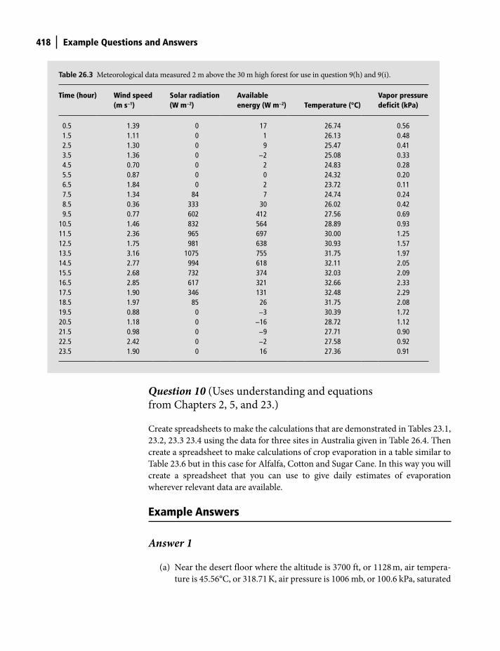
In the following, assume the meteorological data given in Table 26.3 were measured
2 m above the top of the 30 m high forest and that it is acceptable to use the
aerodynamic resistance ra calculated in 9(f) and the formulae for surface
conductance specified in 9(g) to calculate the surface resistance rs (= g
s−1).
(h) Plot the variation through the day of the individual stress functions gR, g
D ,
and gT , and also the total stress function, i.e., the product (g
R g
D g
T g
M).
(i) Using the Penman-Monteith equation (Equation 21.33) and the surface
energy balance, plot the variation through the day of available energy,
latent heat and sensible heat fluxes.
Shuttleworth_c26.indd 417Shuttleworth_c26.indd 417 11/3/2011 6:37:28 PM11/3/2011 6:37:28 PM
418 Example Questions and Answers
Table 26.3 Meteorological data measured 2 m above the 30 m high forest for use in question 9(h) and 9(i).
Time (hour) Wind speed (m s−1)
Solar radiation (W m−2)
Available energy (W m−2) Temperature (°C)
Vapor pressure deficit (kPa)
0.5 1.39 0 17 26.74 0.561.5 1.11 0 1 26.13 0.482.5 1.30 0 9 25.47 0.413.5 1.36 0 −2 25.08 0.334.5 0.70 0 2 24.83 0.285.5 0.87 0 0 24.32 0.206.5 1.84 0 2 23.72 0.117.5 1.34 84 7 24.74 0.248.5 0.36 333 30 26.02 0.429.5 0.77 602 412 27.56 0.69
10.5 1.46 832 564 28.89 0.9311.5 2.36 965 697 30.00 1.2512.5 1.75 981 638 30.93 1.5713.5 3.16 1075 755 31.75 1.9714.5 2.77 994 618 32.11 2.0515.5 2.68 732 374 32.03 2.0916.5 2.85 617 321 32.66 2.3317.5 1.90 346 131 32.48 2.2918.5 1.97 85 26 31.75 2.0819.5 0.88 0 −3 30.39 1.7220.5 1.18 0 −16 28.72 1.1221.5 0.98 0 −9 27.71 0.9022.5 2.42 0 −2 27.58 0.9223.5 1.90 0 16 27.36 0.91
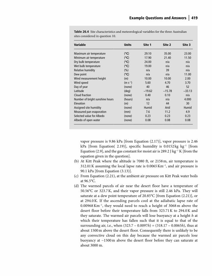
Question 10 (Uses understanding and equations from Chapters 2, 5, and 23.)
Create spreadsheets to make the calculations that are demonstrated in Tables 23.1,
23.2, 23.3 23.4 using the data for three sites in Australia given in Table 26.4. Then
create a spreadsheet to make calculations of crop evaporation in a table similar to
Table 23.6 but in this case for Alfalfa, Cotton and Sugar Cane. In this way you will
create a spreadsheet that you can use to give daily estimates of evaporation
wherever relevant data are available.
Example Answers
Answer 1
(a) Near the desert floor where the altitude is 3700 ft, or 1128 m, air tempera-
ture is 45.56°C, or 318.71 K, air pressure is 1006 mb, or 100.6 kPa, saturated
Shuttleworth_c26.indd 418Shuttleworth_c26.indd 418 11/3/2011 6:37:28 PM11/3/2011 6:37:28 PM
Example Questions and Answers 419
vapor pressure is 9.86 kPa [from Equation (2.17)], vapor pressure is 2.46
kPa [from Equation( 2.19)], specific humidity is 0.0152 kg kg−1 [from
Equation (2.9], and the gas constant for moist air is 289.2 J kg−1 K [from the
equation given in the question].
(b) At Kitt Peak where the altitude is 7080 ft, or 2158 m, air temperature is
312.01 K assuming the local lapse rate is 0.0065 Km−1, and air pressure is
90.1 kPa [from Equation (3.13)].
(c) From Equation (2.21), at the ambient air pressure on Kitt Peak water boils
at 96.5°C.
(d) The warmed parcels of air near the desert floor have a temperature of
50.56°C or 323.7 K, and their vapor pressure is still 2.46 kPa. They will
saturate at a dew point temperature of 20.85°C [from Equation (2.21)], or
at 294.0 K. If the ascending parcels cool at the adiabatic lapse rate of
0.00968 Km−1, they would need to reach a height of 3068 m above the
desert floor before their temperature falls from 323.71 K to 294.0 K and
they saturate. The warmed air parcels will lose buoyancy at a height h at
which their temperature has fallen such that it is equal to that of the
surrounding air, i.e., when (323.7 – 0.0097h) = (318.17 – 0.0065h), thus at
about 1500 m above the desert floor. Consequently there is unlikely to be
any convective cloud on this day because the warmed air parcels lose
buoyancy at ∼1500 m above the desert floor before they can saturate at
about 3000 m.
Table 26.4 Site characteristics and meteorological variables for the three Australian
sites considered in question 10.
Variable Units Site 1 Site 2 Site 3
Maximum air temperature (°C) 29.10 35.00 23.00Minimum air temperature (°C) 17.90 21.40 11.50Dry bulb temperature (°C) 24.00 n/a n/aWet bulb temperature (°C) 19.00 n/a n/aRelative humidity (%) n/a 39 n/aDew point (°C) n/a n/a 11.00Wind measurement height (m) 10.00 10.00 2.00Wind speed (m s−1) 5.60 4.70 3.70Day of year (none) 40 46 52Latitude (deg) −19.62 −15.78 −33.13Cloud fraction (none) 0.40 0.10 n/aNumber of bright sunshine hours (hours) n/a n/a 4.000Elevation (m) 12 44 30Assigned site humidity (none) Humid Arid HumidMeasured pan evaporation (mm) 7.6 11.2 4.9Selected value for Albedo (none) 0.23 0.23 0.23Albedo of open water (none) 0.08 0.08 0.08
Shuttleworth_c26.indd 419Shuttleworth_c26.indd 419 11/3/2011 6:37:29 PM11/3/2011 6:37:29 PM
420 Example Questions and Answers
Answer 2
(a) At this site on this day, the all-day average air temperature is 22°C, or
295.13 K, the saturated vapor pressure is 2.644 kPa, and the vapor pressure
is 1.322 kPa.
(b) When calculating net longwave radiation, the effective emissivity e’ = 0.194
[from Equation (5.23)] and assuming c = 0.7 all through the day, for an arid
site the empirical cloud factor f = 0.37 [from Equation (5..25)]. The esti-
mated all-day average net longwave radiation is therefore –28 W m−2 [from
Equation (5..22)].
(c) Were this a humid site the empirical cloud factor, f, would then be 0.533
[from Equation (5..24)] and the estimated all-day average net longwave
radiation would be -41 W m−2 [from Equation (5..22)].
(d) July 12 is Day Of Year 193, hence the eccentricity factor dl = 0.968 [from
Equation (5.5)] and the solar declination δ = 0.385 radians [from Equation
(5.8)]. The latitude of the site is 32.5°N, which is +0.567 radians, and the
hour angle, w, can be calculated in radians from the time of day, t, in hours
[using Equation (5.10)], with t running in hourly increments from 0.5 to
23.5. Consequently, the solar radiation at the top of the atmosphere, Stop, can
be calculated [from Equation (26.1)] and solar radiation at the ground, Sgrnd,
calculated [from Equation (26.2)]. Values of net solar radiation can then
be calculated for each value of t by allowing for the albedo of 0.23 [by
comparison with Equation (5.18)]. Values of net radiation can then be cal-
culated for each value of t by adding the relevant values of longwave radiation
for arid and humid conditions calculated in sections (b) and (c), respectively.
The resulting values of solar radiation, net solar radiation, and net radiation
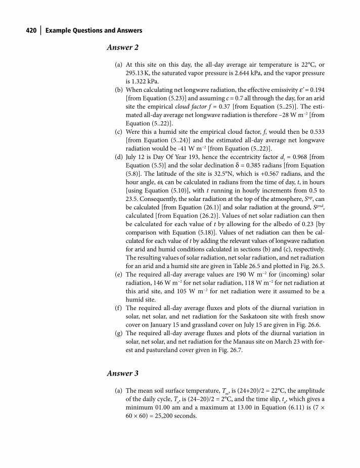
for an arid and a humid site are given in Table 26.5 and plotted in Fig. 26.5.
(e) The required all-day average values are 190 W m−2 for (incoming) solar
radiation, 146 W m−2 for net solar radiation, 118 W m−2 for net radiation at
this arid site, and 105 W m−2 for net radiation were it assumed to be a
humid site.
(f) The required all-day average fluxes and plots of the diurnal variation in
solar, net solar, and net radiation for the Saskatoon site with fresh snow
cover on January 15 and grassland cover on July 15 are given in Fig. 26.6.
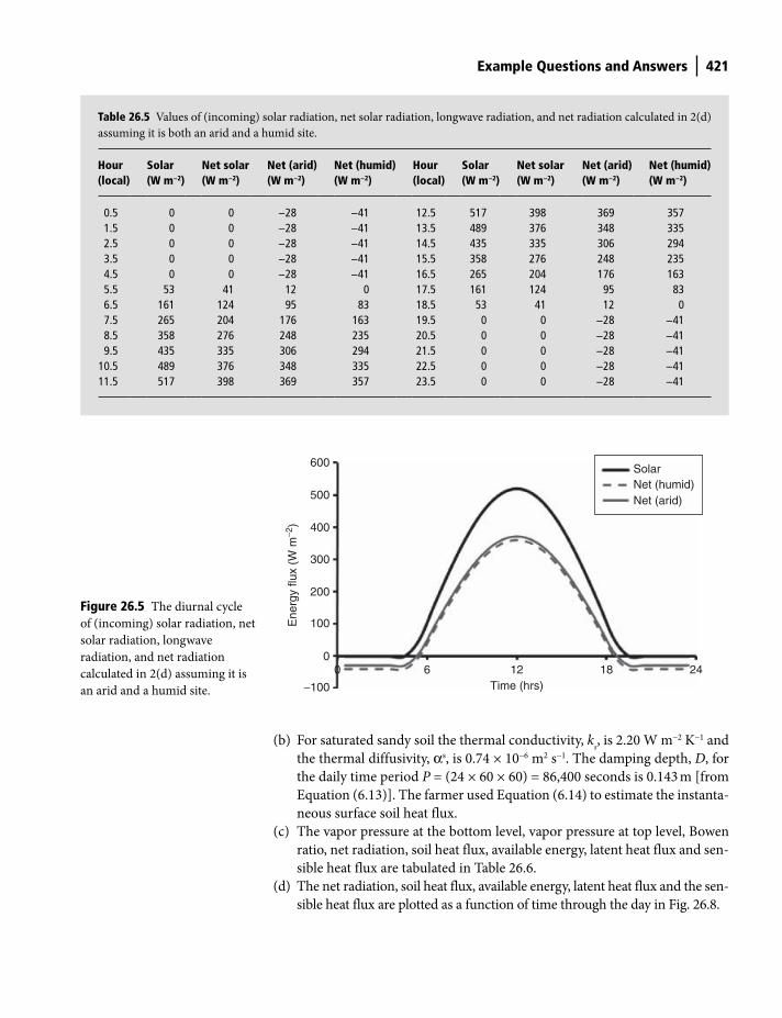
(g) The required all-day average fluxes and plots of the diurnal variation in
solar, net solar, and net radiation for the Manaus site on March 23 with for-
est and pastureland cover given in Fig. 26.7.
Answer 3
(a) The mean soil surface temperature, Tm
, is (24+20)/2 = 22°C, the amplitude
of the daily cycle, Ta, is (24–20)/2 = 2°C, and the time slip, t
o, which gives a
minimum 01.00 am and a maximum at 13.00 in Equation (6.11) is (7 ×
60 × 60) = 25,200 seconds.
Shuttleworth_c26.indd 420Shuttleworth_c26.indd 420 11/3/2011 6:37:29 PM11/3/2011 6:37:29 PM
Example Questions and Answers 421
(b) For saturated sandy soil the thermal conductivity, ks, is 2.20 W m−2 K−1 and
the thermal diffusivity, αs, is 0.74 × 10⁻⁶ m2 s−1. The damping depth, D, for
the daily time period P = (24 × 60 × 60) = 86,400 seconds is 0.143 m [from
Equation (6.13)]. The farmer used Equation (6.14) to estimate the instanta-
neous surface soil heat flux.
(c) The vapor pressure at the bottom level, vapor pressure at top level, Bowen
ratio, net radiation, soil heat flux, available energy, latent heat flux and sen-
sible heat flux are tabulated in Table 26.6.
(d) The net radiation, soil heat flux, available energy, latent heat flux and the sen-
sible heat flux are plotted as a function of time through the day in Fig. 26.8.
60 12Time (hrs)
18 24
Solar
Net (arid)Net (humid)
600
500
400
300
200
100
0
−100
Ene
rgy
flux
(W m
−2)
Figure 26.5 The diurnal cycle
of (incoming) solar radiation, net
solar radiation, longwave
radiation, and net radiation
calculated in 2(d) assuming it is
an arid and a humid site.
Table 26.5 Values of (incoming) solar radiation, net solar radiation, longwave radiation, and net radiation calculated in 2(d)
assuming it is both an arid and a humid site.
Hour (local)
Solar (W m−2)
Net solar (W m−2)
Net (arid) (W m−2)
Net (humid) (W m−2)
Hour (local)
Solar (W m−2)
Net solar (W m−2)
Net (arid) (W m−2)
Net (humid) (W m−2)
0.5 0 0 −28 −41 12.5 517 398 369 3571.5 0 0 −28 −41 13.5 489 376 348 3352.5 0 0 −28 −41 14.5 435 335 306 2943.5 0 0 −28 −41 15.5 358 276 248 2354.5 0 0 −28 −41 16.5 265 204 176 1635.5 53 41 12 0 17.5 161 124 95 836.5 161 124 95 83 18.5 53 41 12 07.5 265 204 176 163 19.5 0 0 −28 −418.5 358 276 248 235 20.5 0 0 −28 −419.5 435 335 306 294 21.5 0 0 −28 −41
10.5 489 376 348 335 22.5 0 0 −28 −4111.5 517 398 369 357 23.5 0 0 −28 −41
Shuttleworth_c26.indd 421Shuttleworth_c26.indd 421 11/3/2011 6:37:29 PM11/3/2011 6:37:29 PM

422 Example Questions and Answers
All-day average values
30
6
−46
−40
Solar (W m−2)
Net solar (W m−2)
Longwave (W m−2)
Net (W m−2)
All-day average values
208
160
−19
141
Solar (W m−2)
Net solar (W m−2)
Longwave (W m−2)
Net (W m−2)
200
150
100
50
0
−50
−100
0 6 12
Time (hrs)
18 24Ene
rgy
flux
(W m
−2)
Solar
Net solar
Net
Saskatoon Jan 15 (fresh snow)
−100
0
100
200
300
400
500
600
Time (hrs)
0 6 12 18 24
Solar
Net solar
Net
Saskatoon Jan 15 (grassland)
Ene
rgy
flux
(W m
−2)
Figure 26.6 Diurnal variation
in all-day average radiation
fluxes calculated in 2(f).
(e) The all-day average values of the Bowen ratio and Evaporative Fraction at
his site are calculated from the all-day average values of latent and sensible
(not by averaging the hourly average values) and are 0.486 and 0.673,
respectively.
Shuttleworth_c26.indd 422Shuttleworth_c26.indd 422 11/3/2011 6:37:30 PM11/3/2011 6:37:30 PM
Example Questions and Answers 423
All-day average values
175
154
−15
139
Solar (W m−2)
Net Solar (W m−2)
Longwave (W m−2)
Net (W m−2)
All-day average values
175
135
−15
120
Solar (W m−2)
Net solar (W m−2)
Longwave (W m−2)
Net (W m−2)
600
500
400
300
200
0
100
−1000 6 12
Time (hrs)18 24
En
erg
y fl
ux
(W m
-2) Solar
Net solar
Net
Manaus March 23 (forest)
−100
0
100
200
300
400
500
600
Time (hrs)
0 6 12 18 24
Solar
Net solar
Net
Manaus March 23 (pasture)
En
erg
y fl
ux
(W m
-2)
Figure 26.7 Diurnal variation
in all-day average radiation
fluxes calculated in 2(g).
(f) Had the farmer neglected soil heat flux he would have estimated greater
available energy during the day when evaporation is the dominant flux,
and less at night when sensible heat is the dominant flux. The net effect
would have been to overestimate the all-day average evaporation flux.
Shuttleworth_c26.indd 423Shuttleworth_c26.indd 423 11/3/2011 6:37:31 PM11/3/2011 6:37:31 PM
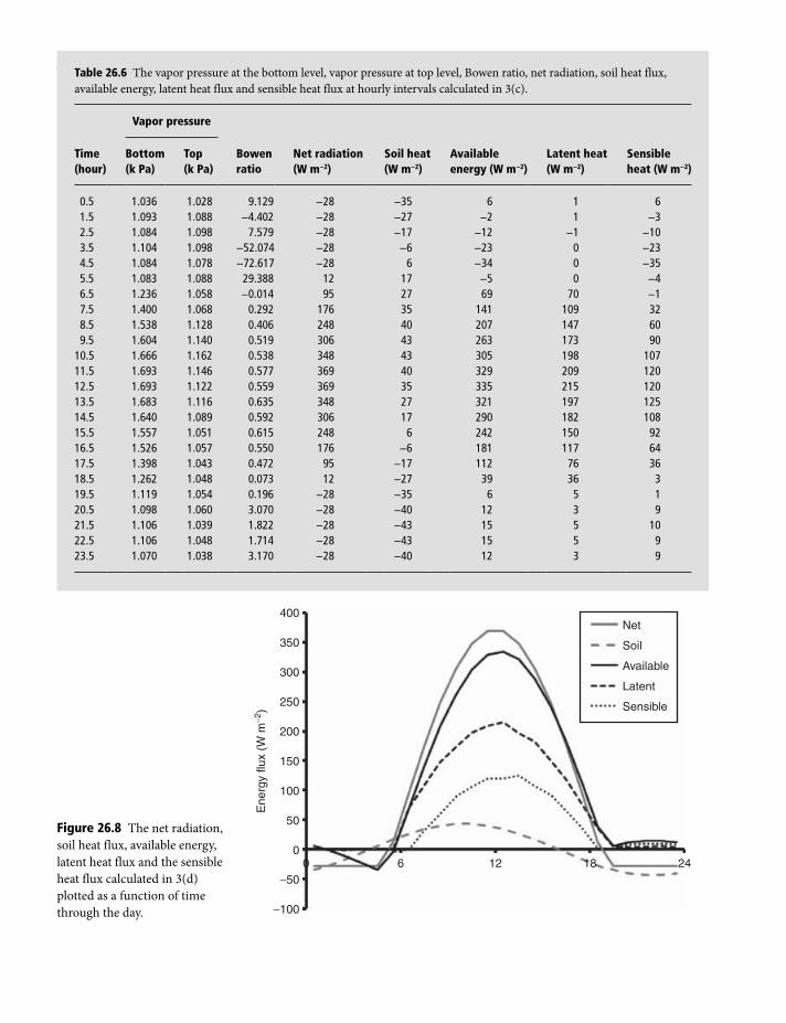
424 Example Questions and AnswersTable 26.6 The vapor pressure at the bottom level, vapor pressure at top level, Bowen ratio, net radiation, soil heat flux,
available energy, latent heat flux and sensible heat flux at hourly intervals calculated in 3(c).
Vapor pressure
Time (hour)
Bottom (k Pa)
Top (k Pa)
Bowen ratio
Net radiation (W m−2)
Soil heat (W m−2)
Available energy (W m−2)
Latent heat (W m−2)
Sensible heat (W m−2)
0.5 1.036 1.028 9.129 −28 −35 6 1 61.5 1.093 1.088 −4.402 −28 −27 −2 1 −32.5 1.084 1.098 7.579 −28 −17 −12 −1 −103.5 1.104 1.098 −52.074 −28 −6 −23 0 −234.5 1.084 1.078 −72.617 −28 6 −34 0 −355.5 1.083 1.088 29.388 12 17 −5 0 −46.5 1.236 1.058 −0.014 95 27 69 70 −17.5 1.400 1.068 0.292 176 35 141 109 328.5 1.538 1.128 0.406 248 40 207 147 609.5 1.604 1.140 0.519 306 43 263 173 90
10.5 1.666 1.162 0.538 348 43 305 198 10711.5 1.693 1.146 0.577 369 40 329 209 12012.5 1.693 1.122 0.559 369 35 335 215 12013.5 1.683 1.116 0.635 348 27 321 197 12514.5 1.640 1.089 0.592 306 17 290 182 10815.5 1.557 1.051 0.615 248 6 242 150 9216.5 1.526 1.057 0.550 176 −6 181 117 6417.5 1.398 1.043 0.472 95 −17 112 76 3618.5 1.262 1.048 0.073 12 −27 39 36 319.5 1.119 1.054 0.196 −28 −35 6 5 120.5 1.098 1.060 3.070 −28 −40 12 3 921.5 1.106 1.039 1.822 −28 −43 15 5 1022.5 1.106 1.048 1.714 −28 −43 15 5 923.5 1.070 1.038 3.170 −28 −40 12 3 9
400
350
300
250
200
150
100
50
0
−50
−100
0 6 12 18 24
Net
Soil
Available
Latent
Sensible
Ene
rgy
flux
(W m
−2)
Figure 26.8 The net radiation,
soil heat flux, available energy,
latent heat flux and the sensible
heat flux calculated in 3(d)
plotted as a function of time
through the day.
Shuttleworth_c26.indd 424Shuttleworth_c26.indd 424 11/3/2011 6:37:31 PM11/3/2011 6:37:31 PM
Example Questions and Answers 425
Answer 4
(a) Shuttleworth is speaking about the annual average evaporation from the
oceanic surfaces of the globe which is about 1.2 m per year. Around 90% of
this water falls back to the ocean while 10% moves and falls over land. When
averaged over all continental surfaces, about 65% of the precipitation falling
over land re-evaporates back to the atmosphere but in semi-arid areas the
proportion is higher. In Arizona, for instance, around 95% re-evaporates.
(b) Shuttleworth is talking about General Circulation models (GCMs). The
two components of these models he is referring to are the dynamics and the
physics. The dynamics applies conservation laws to calculate the fields of
atmospheric variables such as temperature, humidity and wind speed using
prescribed values for the divergence terms in these laws, see Chapters 16
and 17. The physics re-calculates the values of the divergence terms using
the (now modified) fields of atmospheric variables. Some of the processes
represented in the physics include radiation absorption, convection, and
precipitation processes in the atmosphere, and boundary layer and surface
exchange processes
(c) If all the Earth’s continents were clustered at the equator the seasonality of
the global average surface reflection coefficient for solar radiation, i.e. the
global average albedo, might well be less because, being on average warmer
than at present, they would presumably experience less snowfall. The
change in albedo associated with seasonal variations in snow and ice cover
is large because the albedo of fresh snow is around 80% while that for most
natural surfaces is around 20%. Alternative reasons for reduced seasonality
in global albedo include the possibility of reduced seasonal changes in the
vigor of the vegetation covering the continents.
(d) Shuttleworth is referring to the fact that the processes giving rise to
precipitation above, but comparatively close to the Earth’s surface, release
water vapor from the atmosphere and return it to the ground as precipitation,
which at the same time releases latent heat in the atmosphere. On average,
they therefore have the dual effect of reducing the lapse rate in the atmospheric
boundary layer so it is less than the adiabatic lapse rate while simultaneously
ensuring that atmospheric water vapor largely remains fairly near the surface.
(e) Presumably Shuttleworth is talking about GCMs again, because GCMs
have three main applications, namely (i) weather forecasting, (ii) climate
forecasting, and (iii) the synthesis of model-calculated fields of atmos-
pheric and surface variables across the entire globe as a by-product of
application (i). Weather forecasting seeks to predict actual weather a few
days ahead from well-defined initial conditions that may become the data
product (iii). In the case of (ii), initiation is less important because in this
application it is not actual weather but rather the statistics of weather (i.e.,
climate) that is the objective.
(f) Shuttleworth is respectively referring to the specific heat and density of
water relative to that of air. This difference means that the water in oceans
Shuttleworth_c26.indd 425Shuttleworth_c26.indd 425 11/3/2011 6:37:32 PM11/3/2011 6:37:32 PM
426 Example Questions and Answers
absorbs and releases energy more slowly than air and this is the fundamental
basis for the seasonal predictions that are the focus of interest of the Climate
Prediction Center whose website is at http://www.cpc.noaa.gov. Even if
seasonal predictions were not possible, presumably short-term prediction
would still be possible, and weather forecast centers such as the National
Weather Service at http://www.cpc.noaa.gov would still exist.
(g) ‘Greenhouse warming’ is predicted to increase near-surface air tempera-
tures. Since 70% of the Earth is covered with ocean, this likely will increase
surface evaporation rates because the saturated vapor pressure is a strong
function of temperature. Putting more water into the air as water vapor will
likely enhance the Earth’s overall hydrologic cycle by increasing the moisture
available for release by precipitation processes. At first sight, the effect will be
greatest at the poles because the projected temperature increases are greatest
there. However, saturated vapor pressure is a non-linear function of tem-
perature and the rate of change in saturated vapor pressure with temperature
is more than twice as large at 29°C (typical of sea surface temperature at the
equator) than it is at 0°C (typical of sea surface temperature at the poles).
Answer 5
The answers below give one opinion but, as is generally the case in politics,
different people have different opinions. If your opinions differ, discuss them with
your instructor.
(a) The RWD Party is probably using the banner C. Malleable has Hadley
Circulation similar to on Earth. Having looked through a telescope at their
sister planet, RWD Party followers notice that the resulting falling air
currents at approximately 30°N and 30°S of the equator suppress the
formation of precipitation and give rise to warm deserts when this occurs
over continents, e.g. the Sahara Desert. Their proposal is to remove the
continents at this band of latitudes.
(b) The RTS Party is probably using the banner A. The oceans on Malleable are
currently arranged to inhibit the inclusion of cold polar water in oceanic
circulation towards the equator. Looking through a telescope, followers of
the RTS Party notice that on their sister planet Earth, there is a marked
difference in the general shape of continental areas between the two
hemispheres. Those in Earth’s Northern Hemisphere are similar to those
on Malleable and inhibit inclusion of polar water in oceanic circulation.
However, the more open nature of the continents in the Earth’s Southern
Hemisphere allows cold polar water to penetrate towards the equator in the
western Pacific and Atlantic oceans. On average, this reduces the sea
surface temperature of equatorial western oceans in the Earth’s Southern
Hemisphere, and this in turn inhibits the production of tropical storms in
these regions. The RTS Party argues for opening the channels that link
Shuttleworth_c26.indd 426Shuttleworth_c26.indd 426 11/3/2011 6:37:32 PM11/3/2011 6:37:32 PM
Example Questions and Answers 427
polar and tropical oceans on Malleable so as to encourage the inclusion of
colder water towards their planet’s tropical oceans via oceanic circulation.
(c) The MM Party is probably using the banner B. Looking through a telescope,
followers of the MM Party notice that on their sister planet Earth there is
strong hydroclimatic feature that involves a marked seasonal reversal in
wind direction between areas on land and ocean. By listening in to the
radio broadcasts of weather services on Earth they learn this is called a
Monsoon. They notice that when the land surface is preferentially heated
by the shifting axis of rotation of the Sun there is a seasonal flow which
brings moisture over land that falls as precipitation in some months and
this is useful for growing agricultural crops. They also notice the effect is
greater when the flow is between a warm tropical ocean and large areas of
land that have a boundary which lies roughly parallel to the equator, e.g.,
the Indian Ocean and the continent of Asia. They are therefore suggesting
the continents on Malleable are arranged to favor such Monsoon flows.
(d) The RWD Party’s argument for the REN Party forming a coalition with
them is quite strong. They point out that relative to the existing continental
distribution, their proposed redistribution will significantly reduce the
portion of Malleable’s tropical ocean in which the Trade Winds can estab-
lish ‘warm pools’. The REN Party is negotiating for a bigger proportion of
the available land area at the equator but is facing opposition from the more
conservative faction of the RWD Party who have grown up in cooler cli-
mates with marked seasons.
(e) The RTS Party’s argument for the REN Party forming a coalition with them
is also reasonably convincing. They point out that their proposal will much
lessen the distance the Trade Winds have to establish ‘warm pools’ because of
the reduced distance between their four (as opposed to two) continents, and
because each proposed continent has more land area at the equator relative to
the existing continents. The REN party is negotiating for yet more continents
with more of their land area at the equator if they agree to form a coalition.
Answer 6
(a) Solar radiation heats the atmosphere from below, while it heats the oceans
from above. This results in a buoyant mixed layer on the surface of the
oceans which is typically 100–1000 m deep, and separated from the lower
ocean by the thermocline. The oceanic structure is fairly constant in time
in tropical regions, but the mixing layer changes depth with season at mid-
latitudes, being shallower and warmer in summer months when surface
heating is greater and the ensuing buoyancy of the surface water is greater.
(b) The student was a ‘Northo-centralist’ and was wrong. She should have said
‘ocean currents tend to go away from the equator on the eastern sides of
continents, and towards the equator on the western side of continents.’
(c) The near-surface mixed layer circulation of the oceans is primarily influ-
enced by the prevailing low level wind fields. The ocean, being massive, in
Shuttleworth_c26.indd 427Shuttleworth_c26.indd 427 11/3/2011 6:37:32 PM11/3/2011 6:37:32 PM
428 Example Questions and Answers
effect acts like a filter, picking out and following the average wind flow. Sea
water tends to be blown easterly near the equator and westerly at mid-lati-
tudes, and the near-continent currents are formed as part of this circula-
tion. But nothing is quite that simple in the global system and thermocline
circulation caused by changes in density, mainly salt concentration, and
Coriolis acceleration also play a role.
(d) This is actually a very complex problem, but shape of the land masses sur-
rounding oceans clearly influence the surface currents of oceans. In par-
ticular, the presence of substantial land at high latitude tends to inhibit the
linkage between (say) the Atlantic Ocean and cold polar waters, see answer
7(b). South America and Africa tend to taper towards the south pole
(unlike in the north Atlantic) and there is little land south of 40 degrees
south. The Benguela current in the South Atlantic (like the Peru current in
the Pacific) can access cold polar water more easily than the Canary current
in the North Atlantic, and this results in a lower SST at about 10-20 degrees
from the equator in the eastern portion of the ocean.
Tropical storms and hurricanes are formed in a region about 10–20 degrees
north and south of the equator (because there is not enough Coriolis force
at the very low latitude), and initially tend to move east to west in the
prevailing Trade Winds. The SST in central and eastern portions of 10–20
degrees north of the equator in the Atlantic is warmer than the 26.5 degrees
required for formation of tropical cyclones for a substantial portion of the
year, and the islands of the Caribbean suffer in consequence. But south of
the equator the equivalent phenomenon is suppressed by the cooler SST in
the eastern tropical Atlantic, and partly because of this and partly because
it is nearer to the equator, the climate of northeastern Brazil, though still
subject to oceanic influence, is spared.
(e) The student realized that the relative proportion of surface radiation used
to evaporate water over the oceans is greater than over land where more is
used to warm the lower atmosphere. The yearly cycle in near-surface tem-
perature is therefore greater over land surfaces than it is over oceans, and
this seasonal temperature differential (between the Asian continent and the
Indian ocean) is the driving mechanism behind the South East Asian mon-
soon, which is a major hydroclimatological influence on that region of the
world where a large portion of human population is concentrated.
(f) For clouds to occur not only must there be a mechanism that gives ascent
and cooling, but there must also be (i) sufficient moisture available in the
atmosphere, and (ii) cloud condensation nuclei (CCN) for cloud droplets
to form around. However, there are usually enough CCN available in the
air hence, choosing between these two, moisture availability is probably the
limiting requirement. However, quite often the atmosphere has both
enough CCN and enough moisture and the absence of an atmospheric
ascent mechanism is then the limiting criterion.
(g) The molecular weight of water molecules is less than the average molecular
weight of the mixture of oxygen and nitrogen molecules that make up dry
Shuttleworth_c26.indd 428Shuttleworth_c26.indd 428 11/3/2011 6:37:32 PM11/3/2011 6:37:32 PM
Example Questions and Answers 429
air. At the same temperature and pressure, the moister air has the same
number of molecules as the drier air, but some of the heavier air molecules
are replaced by lighter vapor molecules. Rearranging the Ideal Gas Law for
moist air, gives:
ra = [P/(R
d T)] / [1 + 0.61(r
v / r
a )] = [P/(R
d T)] / [1 + 0.61q]
Rd is a constant so assuming the temperature and pressure are the same, if
a parcel of air is moister than its surroundings (i.e. if q is greater) its density
is less than the surrounding air and it will tend to rise. It is the effect of
this greater buoyancy which is allowed for by re-expressing potential
temperature as virtual potential temperature.
(h) In convective conditions parcels of air heated to a temperature above that
of the surrounding atmosphere near the ground can often keep on rising to
the cloud condensation level because both the air in the parcel and the sur-
rounding air cool with height. However, the ascending air cools at the dry
adiabatic lapse rate and the surrounding air cools less quickly so there can
be situations where ascent is suppressed prior to reaching the level at which
water vapor in the rising air parcels saturates, see answer 1(d).
(i) Once at the cloud condensation level, condensation and cloud formation
begins. This releases latent heat which further warms the air thus tending
to make the air more buoyant and enhancing its further ascent within the
cloud.
(j) In mid-latitude clouds with a temperature of –25°C all the phases of water
(solid, liquid or vapor) are likely to be present. In such clouds the Bergeron-
Findeison process is likely to be the most important process responsible for
cloud particle growth.
Answer 7
(a) Very open situations are not necessarily always the best rain gauge sites
because near-ground wind speeds tend to be higher and wind-related
blow-in/blow-out gauge errors possibly higher. Consequently an optimum
site might be surrounded by obstructions but should be located in a flat
open area of short mown grass and should be sufficiently far from up-wind
of obstructions that they all subtend a vertical angle of less than 30°. Ideally,
the gauge would be placed at the center of a pit in the ground (say) 1–2 m
across such that the top of the gauge is level with the ground. This avoids
splash-in errors. The top of the pit should be covered with an open mesh
(plastic mesh is cheap and easy to find) so that it has a similar aerody-
namic roughness to that of the surrounding grass. If this is done the near-
surface wind flow is essentially parallel to the ground and the effect of
wind on the gauge is minimized. Such a site might look like that shown
in Fig. 26.9.
Shuttleworth_c26.indd 429Shuttleworth_c26.indd 429 11/3/2011 6:37:32 PM11/3/2011 6:37:32 PM
430 Example Questions and Answers
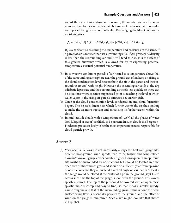
(b) Over the period 1961–1990 the monthly average precipitation for the
months January through December for Tucson were 0.87, 0.7, 0.72, 0.30,
0.18, 0.20, 2.35, 2.19, 0.67, and 1.07 inches, respectively. The seasonality
index calculated using Equation (13.1) from these values is 0.55, which
implies a rainfall regime that is fairly seasonal.
(c) The monthly average precipitation for the months January through
December for Tucson given in (b) are plotted as a pie diagram in Fig. 26.10.
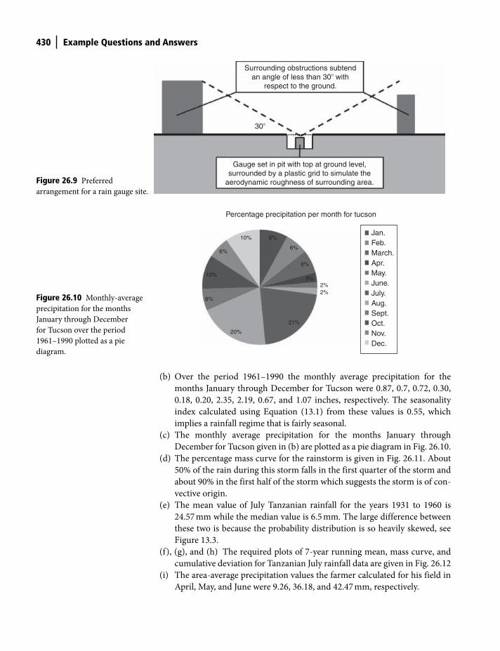
(d) The percentage mass curve for the rainstorm is given in Fig. 26.11. About
50% of the rain during this storm falls in the first quarter of the storm and
about 90% in the first half of the storm which suggests the storm is of con-
vective origin.
(e) The mean value of July Tanzanian rainfall for the years 1931 to 1960 is
24.57 mm while the median value is 6.5 mm. The large difference between
these two is because the probability distribution is so heavily skewed, see
Figure 13.3.
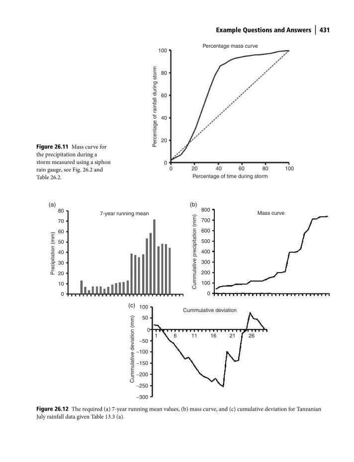
(f), (g), and (h) The required plots of 7-year running mean, mass curve, and
cumulative deviation for Tanzanian July rainfall data are given in Fig. 26.12
(i) The area-average precipitation values the farmer calculated for his field in
April, May, and June were 9.26, 36.18, and 42.47 mm, respectively.
Surrounding obstructions subtendan angle of less than 30� with
respect to the ground.
Gauge set in pit with top at ground level,surrounded by a plastic grid to simulate the
aerodynamic roughness of surrounding area.
30�
Figure 26.9 Preferred
arrangement for a rain gauge site.
Figure 26.10 Monthly-average
precipitation for the months
January through December
for Tucson over the period
1961–1990 plotted as a pie
diagram.
2%3%
6%
6%
8%10%
6%
10%
6%
20%
21%
2%
Percentage precipitation per month for tucson
Jan.Feb.March.Apr.May.June.July.Aug.Sept.Oct.Nov.Dec.
Shuttleworth_c26.indd 430Shuttleworth_c26.indd 430 11/3/2011 6:37:32 PM11/3/2011 6:37:32 PM
Example Questions and Answers 431
00
20
40
60
80
100
20 40 60
Percentage of time during storm
Percentage mass curve
80 100
Per
cent
age
of r
ainf
all d
urin
g st
orm
Figure 26.11 Mass curve for
the precipitation during a
storm measured using a siphon
rain gauge, see Fig. 26.2 and
Table 26.2.
7-year running mean80(a) (b)
(c)
70
60
50
40
30
20
10
0
Pre
cipi
tatio
n (m
m)
Mass curve800
700
600
500
400
300
200
100
0
Cum
mul
ativ
e pr
ecip
itatio
n (m
m)
Cummulative deviation100
50
0
−50
−100
−150
−200
−250
−300
1 6 11 16 21 26
Cum
mul
ativ
e de
viat
ion
(mm
)
Figure 26.12 The required (a) 7-year running mean values, (b) mass curve, and (c) cumulative deviation for Tanzanian
July rainfall data given Table 13.3 (a).
Shuttleworth_c26.indd 431Shuttleworth_c26.indd 431 11/3/2011 6:37:33 PM11/3/2011 6:37:33 PM
432 Example Questions and Answers
Answer 8
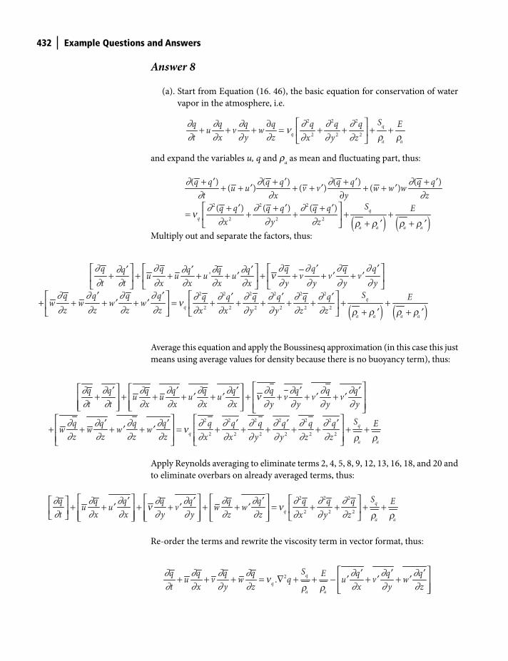
(a). Start from Equation (16. 46), the basic equation for conservation of water
vapor in the atmosphere, i.e.
∂ ∂ ∂ ∂ ∂ ∂ν∂ ∂ ∂ ∂ ∂ ∂ ∂
⎡ ⎤∂+ + + = + + + +⎢ ⎥
⎣ ⎦
2 2 2
2 2 2
a a
Sq q q q q q q Eu v wt x y z x y z r r
and expand the variables u, q and ra as mean and fluctuating part, thus:
( ) ( )
∂ ∂ ∂ ∂∂ ∂ ∂
∂ ∂ ∂∂ ∂ ∂
+ ′ + ′ + ′ + ′+ + ′ + + ′ + + ′
∂⎡ ⎤+ ′ + ′ + ′
= + + + +⎢ ⎥+ ′ + ′⎣ ⎦
2 2 2
2 2 2
( ) ( ) ( ) ( )( ) ( ) ( )
a a a a
q q q q q q q qu u v v w w wt x y z
Sq q q q q q Ex y z
nr r r r
Multiply out and separate the factors, thus:
( ) ( )2 2 2 2 2 2
2 2 2 2 2 2
'
a a a a
q q q q q qq q q qu u u u v v vt t x x x x y y y y
Sq q q q q q q q q q Ew w w wz z z z x x y y z z
′ ′⎡ ⎤ ⎡ ⎤ ⎡ ⎤′ ′ ′+ + + + + ′ + + + ′ + ′⎢ ⎥ ⎢ ⎥ ⎢ ⎥
⎣ ⎦ ⎣ ⎦ ⎣ ⎦′ ′ ⎡ ⎤⎡ ⎤ ′ ′ ′
+ + + ′ + ′ = + + + + + + +⎢ ⎥⎢ ⎥+ ′ + ′⎣ ⎦ ⎣ ⎦
∂ ∂ ∂ ∂ ∂ ∂∂ ∂ ∂ ∂∂ ∂ ∂ ∂ ∂ ∂ ∂ ∂ ∂ ∂
∂ ∂ ∂ ∂ ∂ ∂ ∂ ∂ ∂ ∂∂ ∂ ∂ ∂ ∂ ∂ ∂ ∂ ∂ ∂
n
nr r r r
Average this equation and apply the Boussinesq approximation (in this case this just
means using average values for density because there is no buoyancy term), thus:
∂ ∂ ∂ ∂ ∂ ∂ ∂ ∂ ∂ ∂∂ ∂ ∂ ∂ ∂ ∂ ∂ ∂ ∂ ∂
∂ ∂ ∂ ∂ ∂ ∂ ∂ ∂ ∂ ∂∂ ∂ ∂ ∂ ∂ ∂ ∂ ∂ ∂ ∂
⎡ ⎤⎡ ⎤ ⎡ ⎤′ ′ ′ ′ ′⎢ ⎥+ + + + ′ + ′ + + + ′ + ′⎢ ⎥ ⎢ ⎥⎢ ⎥⎢ ⎥ ⎢ ⎥⎣ ⎦ ⎣ ⎦ ⎣ ⎦
⎡ ⎤ ⎡ ⎤′ ′ ′ ′ ′⎢ ⎥ ⎢ ⎥+ + + ′ + ′ = + + + + + + +⎢ ⎥ ⎢ ⎥⎣ ⎦ ⎣ ⎦
2 2 2 2 2 2
2 2 2 2 2 2
a a
q q q q q q q q q qu u u u v v vt t x x x x y y y y
Sq q q q q q q q q q Ew w w wz z z z x x y y z z
n
nr r
Apply Reynolds averaging to eliminate terms 2, 4, 5, 8, 9, 12, 13, 16, 18, and 20 and
to eliminate overbars on already averaged terms, thus:
∂ ∂ ∂ ∂ ∂ ∂ ∂ ∂ ∂ ∂∂ ∂ ∂ ∂ ∂ ∂ ∂ ∂ ∂ ∂
⎡ ⎤ ⎡ ⎤ ⎡ ⎤ ⎡ ⎤′ ′ ′⎡ ⎤ + + ′ + + ′ + + ′ = + + + +⎢ ⎥ ⎢ ⎥ ⎢ ⎥ ⎢ ⎥⎢ ⎥⎣ ⎦ ⎢ ⎥ ⎢ ⎥ ⎢ ⎥ ⎣ ⎦⎣ ⎦ ⎣ ⎦ ⎣ ⎦
2 2 2
2 2 2
a a
Sq q q q q q q q q q Eu u v w wt x x y y z z x y z
n nr r
Re-order the terms and rewrite the viscosity term in vector format, thus:
∂ ∂ ∂ ∂ ∂ ∂ ∂∂ ∂ ∂ ∂ ∂ ∂ ∂
⎡ ⎤′ ′ ′+ + + = ∇ + + − ′ + ′ + ′⎢ ⎥
⎢ ⎥⎣ ⎦2.
a a
Sq q q q q q qEu v w q u v wt x y z x y z
nr r
Shuttleworth_c26.indd 432Shuttleworth_c26.indd 432 11/3/2011 6:37:33 PM11/3/2011 6:37:33 PM
Example Questions and Answers 433
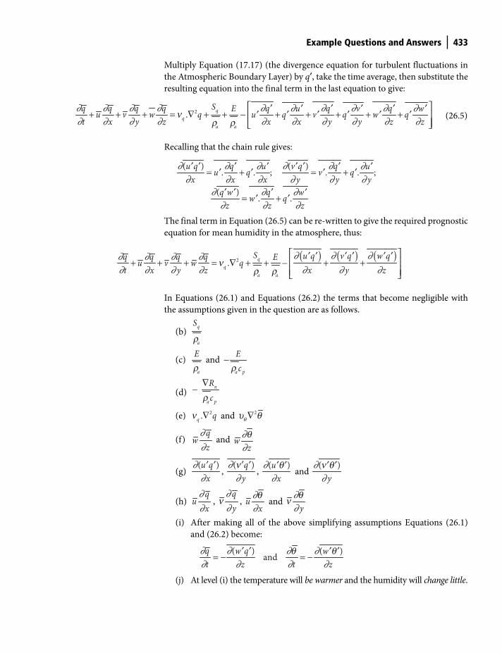
Multiply Equation (17.17) (the divergence equation for turbulent fluctuations in
the Atmospheric Boundary Layer) by q′, take the time average, then substitute the
resulting equation into the final term in the last equation to give:
( ) ( ) ( )∂ ∂ ∂∂ ∂ ∂ ∂∂ ∂ ∂ ∂ ∂ ∂ ∂
⎡ ⎤′ ′ ′ ′ ′ ′⎢ ⎥+ + + = ∇ + + − + +⎢ ⎥⎣ ⎦
2.q
qa a
S u q v q w qq q q q Eu v w qt x y z x y z
nr r
In Equations (26.1) and Equations (26.2) the terms that become negligible with
the assumptions given in the question are as follows.
(b) q
a
S
r
(c) a
Er
and −a p
Ecr
(d) ∇
− n
a p
Rcr
(e) ∇2.q qn and ∇2
qu q
(f) ∂∂q
wz
and ∂∂
wzq
(g) ∂
∂′ ′( )u qx
, ∂
∂′ ′( )qy
n,
∂∂
′ ′( )uxq
and ∂
∂′ ′( )
yn q
(h) ∂∂q
ux
, ∂∂qy
n , ∂∂
uxq
and ∂∂ yq
n
(i) After making all of the above simplifying assumptions Equations (26.1)
and (26.2) become:
∂ ∂ ∂ ∂∂ ∂ ∂ ∂
′ ′ ′ ′= − = −
( ) ( )and
q w q wt z t z
q q
(j) At level (i) the temperature will be warmer and the humidity will change little.
Recalling that the chain rule gives:
∂ ∂ ∂ ∂∂ ∂∂ ∂ ∂ ∂ ∂ ∂
∂ ∂ ∂∂ ∂ ∂
′ ′ ′ ′ ′ ′′ ′= ′ + ′ = ′ + ′
′ ′ ′ ′= ′ + ′
( ) ( ). . ; . . ;
( ). .
u q q v q qu uu q v qx x x y y y
q w q ww qz z z
The final term in Equation (26.5) can be re-written to give the required prognostic
equation for mean humidity in the atmosphere, thus:
∂ ∂ ∂ ∂ ∂ ∂ ∂∂ ∂ ∂∂ ∂ ∂ ∂ ∂ ∂ ∂ ∂ ∂ ∂
⎡ ⎤′ ′ ′′ ′ ′+ + + = ∇ + + − ′ + ′ + ′ + ′ + ′ + ′⎢ ⎥
⎢ ⎥⎣ ⎦2.
a a
Sq q q q q q qE u v wu v w q u q v q w qt x y z x x y y z z
nr r
(26.5)
Shuttleworth_c26.indd 433Shuttleworth_c26.indd 433 11/3/2011 6:37:39 PM11/3/2011 6:37:39 PM
434 Example Questions and Answers
(k) At level (ii) the temperature will be warmer and the humidity will change
little.
(l) At level (iii) the temperature will be warmer and the humidity will change
little.
(m) At level (iv) the temperature will be cooler and the humidity will be wetter.
(n) At level (v) the temperature will change little and the humidity will change
little.
Answer 9
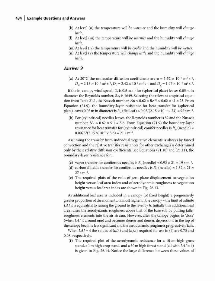
(a) At 20°C the molecular diffusion coefficients are υ = 1.52 × 10⁻⁵ m2 s−1,
DH = 2.15 × 10⁻⁵ m2 s−1, D
V = 2.42 × 10⁻⁵ m2 s−1, and D
C = 1.47 × 10⁻⁵ m2 s−1.
If the in-canopy wind speed, U, is 0.5 m s−1 for (spherical plate) leaves 0.05 m in
diameter the Reynolds number, Re, is 1649. Selecting the relevant empirical equa-
tion from Table 21.1, the Nusselt number, Nu ≈ 0.62 × Re 0.5 ≈ 0.62 × 41 ≈ 25. From
Equation (21.9), the boundary-layer resistance for heat transfer for (spherical
plate) leaves 0.05 m in diameter is RH (flat leaf) ≈ 0.05/(2.15 × 10 −5 × 24) ≈ 92 s m−1.
(b) For (cylindrical) needles leaves, the Reynolds number is 82 and the Nusselt
number, Nu ≈ 0.62 × 9.1 ≈ 5.6. From Equation (21.9) the boundary-layer
resistance for heat transfer for (cylindrical) conifer needles is RH (needle) ≈
0.0025/(2.15 × 10−5 × 5.6) ≈ 21 s m−1.
Assuming the transfer from individual vegetative elements is always by forced
convection and the relative transfer resistances for other exchanges is determined
only by their relative diffusion coefficients, see Equations (21.10) and (21.11), the
boundary-layer resistance for:
(c) vapor transfer for coniferous needles is RV (needle) ≈ 0.93 × 21 ≈ 19 s m−1.
(d) carbon dioxide transfer for coniferous needles is RC (needle) ≈ 1.32 × 21 ≈
27 s m−1.
(e) The required plots of the ratio of zero plane displacement to vegetation
height versus leaf area index and of aerodynamic roughness to vegetation
height versus leaf area index are shown in Fig. 26.13.
As additional leaf area is included in a canopy (of fixed height) a progressively
greater proportion of the momentum is lost higher in the canopy – the limit of infinite
LAI it is equivalent to raising the ground to the level by h. Initially this additional leaf
area raises the aerodynamic roughness above that of the bare soil by putting taller
roughness elements into the air stream. However, after the canopy begins to ‘close’
(when LAI is around one) and becomes denser and denser, depressions in the top of
the canopy become less significant and the aerodynamic roughness progressively falls.
When LAI = 4 the values of (d/h) and (zo/h) required for use in (f) are 0.73 and
0.08, respectively.
(f) The required plot of the aerodynamic resistance for a 10 cm high grass
stand, a 1 m high crop stand, and a 30 m high forest stand (all with LAI = 4)
is given in Fig. 26.14. Notice the large difference between these values of
Shuttleworth_c26.indd 434Shuttleworth_c26.indd 434 11/3/2011 6:37:58 PM11/3/2011 6:37:58 PM
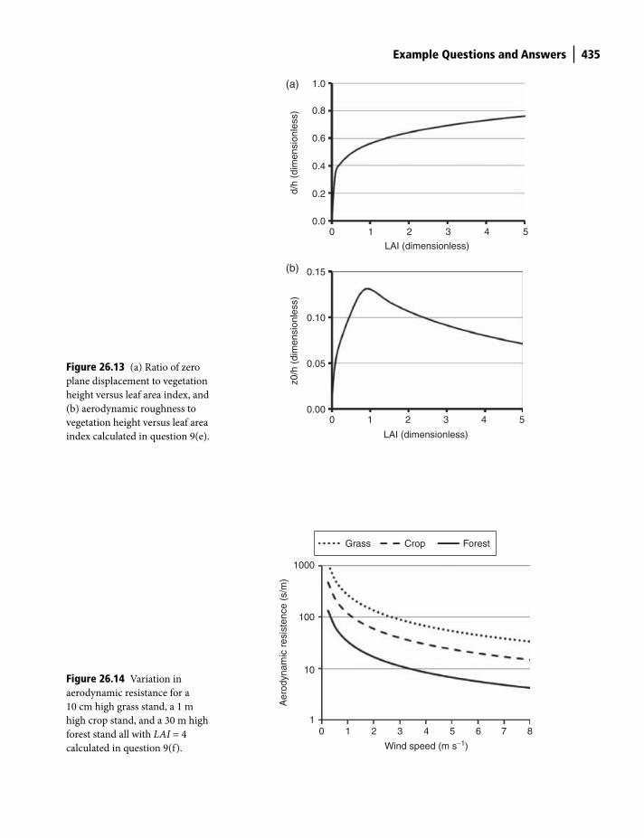
Example Questions and Answers 435
2
LAI (dimensionless)
3 4 5
1.0(a)
(b)
0.8
0.6
0.4
0.2
0.00 1
d/h
(dim
ensi
onle
ss)
2
LAI (dimensionless)
3 4 5
0.15
0.10
0.05
0.000 1
z0/h
(di
men
sion
less
)
Figure 26.13 (a) Ratio of zero
plane displacement to vegetation
height versus leaf area index, and
(b) aerodynamic roughness to
vegetation height versus leaf area
index calculated in question 9(e).
0 1 2 3 4
Wind speed (m s−1)
5 6 7 81
10
100
1000
Aer
odyn
amic
res
iste
nce
(s/m
)
Grass Crop Forest
Figure 26.14 Variation in
aerodynamic resistance for a
10 cm high grass stand, a 1 m
high crop stand, and a 30 m high
forest stand all with LAI = 4
calculated in question 9(f).
Shuttleworth_c26.indd 435Shuttleworth_c26.indd 435 11/3/2011 6:37:58 PM11/3/2011 6:37:58 PM
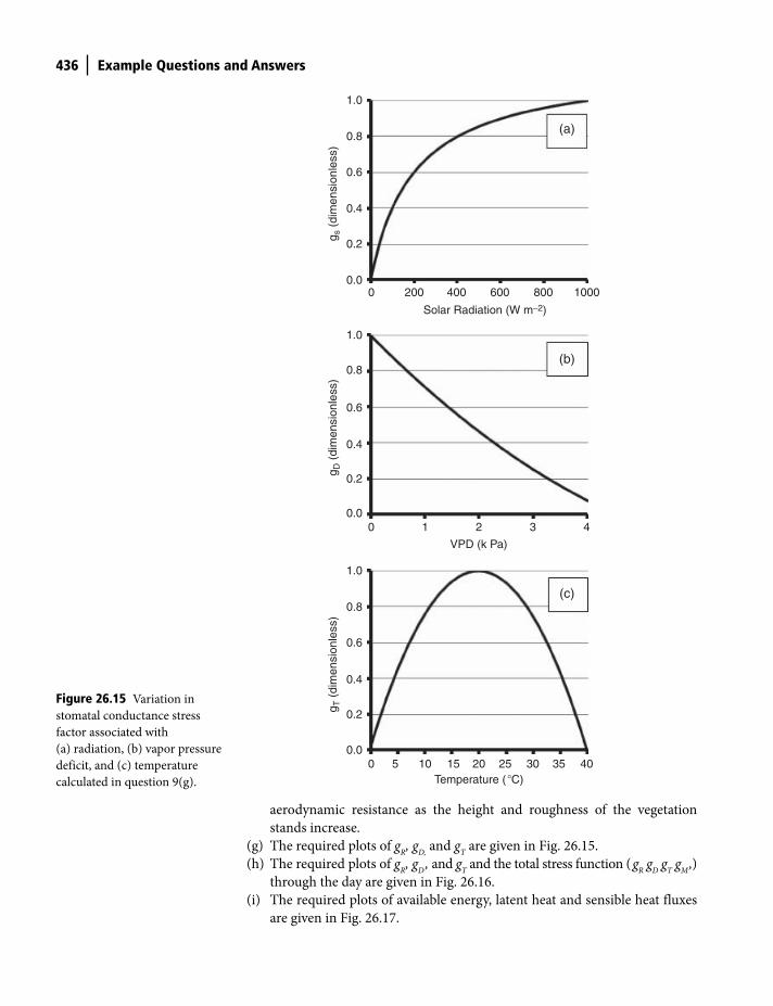
436 Example Questions and Answers
aerodynamic resistance as the height and roughness of the vegetation
stands increase.
(g) The required plots of gR, g
D, and g
T are given in Fig. 26.15.
(h) The required plots of gR, g
D , and g
T and the total stress function ( g
R g
D g
T g
M ,)
through the day are given in Fig. 26.16.
(i) The required plots of available energy, latent heat and sensible heat fluxes
are given in Fig. 26.17.
1.0
0.8
0.6
0.4
0.2
0.0
g s (
dim
ensi
onle
ss)
0 200 400 600 800 1000
1.0
0.8
0.6
0.4
0.2
0.0
g D (
dim
ensi
onle
ss)
0 1 2
VPD (k Pa)
3 4
1.0
0.8
0.6
0.4
0.2
0.0
g T (
dim
ensi
onle
ss)
0 105 20 2515Temperature ( �C)
30 4035
Solar Radiation (W m−2)
(c)
(b)
(a)
Figure 26.15 Variation in
stomatal conductance stress
factor associated with
(a) radiation, (b) vapor pressure
deficit, and (c) temperature
calculated in question 9(g).
Shuttleworth_c26.indd 436Shuttleworth_c26.indd 436 11/3/2011 6:37:58 PM11/3/2011 6:37:58 PM
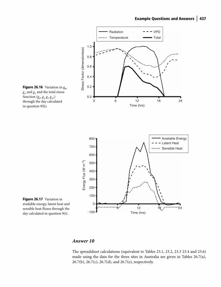
Example Questions and Answers 437
Answer 10
The spreadsheet calculations (equivalent to Tables 23.1, 23.2, 23.3 23.4 and 23.6)
made using the data for the three sites in Australia are given in Tables 26.7(a),
26.7(b), 26.7(c), 26.7(d), and 26.7(e), respectively.
1.0
0.8
0.6
0.4
0.2
0.00 6 12
Time (hrs)18 24
Radiation
Temperature
VPD
Total
Str
ess
Fac
tor
(dim
ensi
onle
ss)
Figure 26.16 Variation in gR,
gD and g
T and the total stress
function (gR, g
D g
T g
M,)
through the day calculated
in question 9(h).
800
700
600
500
400
300
200
100
0
−1000 6 12
Time (hrs)
18 24
Available EnergyLatent Heat
Sensible Heat
Ene
rgy
Flu
x (W
m−2
)
Figure 26.17 Variation in
available energy, latent heat and
sensible heat fluxes through the
day calculated in question 9(i).
Shuttleworth_c26.indd 437Shuttleworth_c26.indd 437 11/3/2011 6:37:59 PM11/3/2011 6:37:59 PM
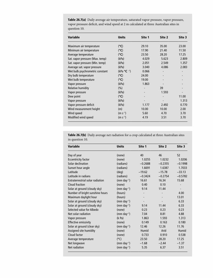
Table 26.7(b) Daily average net radiation for a crop calculated at three Australian sites
in question 10.
Variable Units Site 1 Site 2 Site 3
Day of year (none) 40 46 52Eccentricity factor (none) 1.0255 1.0232 1.0206Solar declination (radians) −0.2688 −0.2355 −0.1998Sunset hour angle (radians) 1.6691 1.6387 1.7033Latitude (deg) −19.62 −15.78 −33.13Latitude in radians (radians) −0.3424 −0.2754 −0.5782Extraterrestrial solar radiation (mm day−1) 16.61 16.34 15.68Cloud fraction (none) 0.40 0.10 -Solar at ground (cloudy sky) (mm day−1) 9.14 11.44 -Number of bright sunshine hours (hours) - - 4.00Maximum daylight hour (hours) - - 13.01Solar at ground (cloudy sky) (mm day−1) - - 6.33Solar at ground (cloudy sky) (mm day−1) 9.14 11.44 6.33Selected value for Albedo (none) 0.23 0.23 0.23Net solar radiation (mm day−1) 7.04 8.81 4.88Vapor pressure (k Pa) 1.863 1.593 1.313Effective emissivity (none) 0.149 0.163 0.180Solar at ground (clear sky) (mm day−1) 12.46 12.26 11.76Assigned site humidity (none) Humid Arid HumidCloud factor (none) 0.733 0.910 0.538Average temperature (°C) 23.50 28.20 17.25Net longwave (mm day−1) −1.68 −2.44 −1.37Net radiation (mm day−1) 5.35 6.37 3.51
Table 26.7(a) Daily average air temperature, saturated vapor pressure, vapor pressure,
vapor pressure deficit, and wind speed at 2 m calculated at three Australian sites in
question 10.
Variable Units Site 1 Site 2 Site 3
Maximum air temperature (°C) 29.10 35.00 23.00Minimum air temperature (°C) 17.90 21.40 11.50Average temperature (°C) 23.50 28.20 17.25Sat. vapor pressure (Max. temp) (kPa) 4.029 5.623 2.809Sat. vapor pressure (Min. temp) (kPa) 2.051 2.549 1.357Average sat. vapor pressure (kPa) 3.040 4.086 2.083Wet bulb psychrometric constant (kPa °C −1) 0.066 - -Dry bulb temperature (°C) 24.00 - -Wet bulb temperature (°C) 19.00 - -Vapor pressure (kPa) 1.863 - -Relative humidity (%) - 39 -Vapor pressure (kPa) - 1.593 -Dew point (°C) - - 11.00Vapor pressure (kPa) - - 1.313Vapor pressure deficit (kPa) 1.177 2.492 0.770Wind measurement height (m) 10.00 10.00 2.00Wind speed (m s−1) 5.60 4.70 3.70Modified wind speed (m s−1) 4.19 3.51 3.70
Shuttleworth_c26.indd 438Shuttleworth_c26.indd 438 11/3/2011 6:37:59 PM11/3/2011 6:37:59 PM
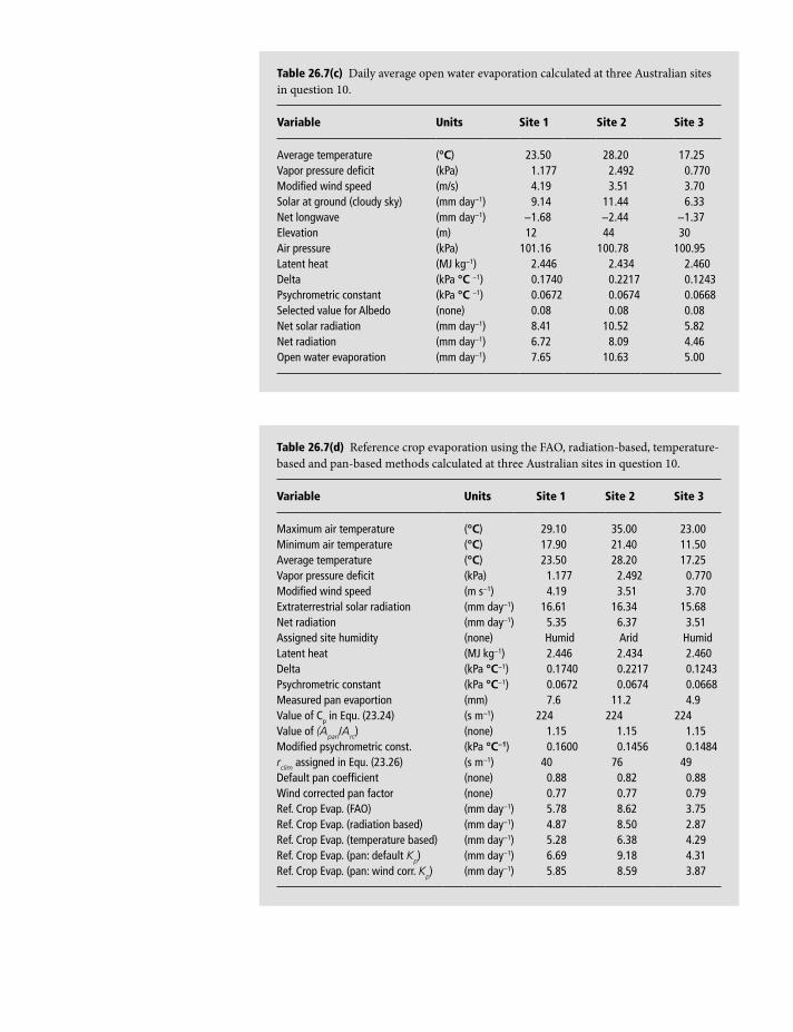
Table 26.7(c) Daily average open water evaporation calculated at three Australian sites
in question 10.
Variable Units Site 1 Site 2 Site 3
Average temperature (°C) 23.50 28.20 17.25Vapor pressure deficit (kPa) 1.177 2.492 0.770Modified wind speed (m/s) 4.19 3.51 3.70Solar at ground (cloudy sky) (mm day−1) 9.14 11.44 6.33Net longwave (mm day−1) −1.68 −2.44 −1.37Elevation (m) 12 44 30Air pressure (kPa) 101.16 100.78 100.95Latent heat (MJ kg−1) 2.446 2.434 2.460Delta (kPa °C −1) 0.1740 0.2217 0.1243Psychrometric constant (kPa °C −1) 0.0672 0.0674 0.0668Selected value for Albedo (none) 0.08 0.08 0.08Net solar radiation (mm day−1) 8.41 10.52 5.82Net radiation (mm day−1) 6.72 8.09 4.46Open water evaporation (mm day−1) 7.65 10.63 5.00
Table 26.7(d) Reference crop evaporation using the FAO, radiation-based, temperature-
based and pan-based methods calculated at three Australian sites in question 10.
Variable Units Site 1 Site 2 Site 3
Maximum air temperature (°C) 29.10 35.00 23.00Minimum air temperature (°C) 17.90 21.40 11.50Average temperature (°C) 23.50 28.20 17.25Vapor pressure deficit (kPa) 1.177 2.492 0.770Modified wind speed (m s−1) 4.19 3.51 3.70Extraterrestrial solar radiation (mm day−1) 16.61 16.34 15.68Net radiation (mm day−1) 5.35 6.37 3.51Assigned site humidity (none) Humid Arid HumidLatent heat (MJ kg−1) 2.446 2.434 2.460Delta (kPa °C−1) 0.1740 0.2217 0.1243Psychrometric constant (kPa °C−1) 0.0672 0.0674 0.0668Measured pan evaportion (mm) 7.6 11.2 4.9Value of Cp in Equ. (23.24) (s m−1) 224 224 224Value of (Apan/Arc) (none) 1.15 1.15 1.15Modified psychrometric const. (kPa °C−1) 0.1600 0.1456 0.1484rclim assigned in Equ. (23.26) (s m−1) 40 76 49Default pan coefficient (none) 0.88 0.82 0.88Wind corrected pan factor (none) 0.77 0.77 0.79Ref. Crop Evap. (FAO) (mm day−1) 5.78 8.62 3.75Ref. Crop Evap. (radiation based) (mm day−1) 4.87 8.50 2.87Ref. Crop Evap. (temperature based) (mm day−1) 5.28 6.38 4.29Ref. Crop Evap. (pan: default Kp) (mm day−1) 6.69 9.18 4.31Ref. Crop Evap. (pan: wind corr. Kp) (mm day−1) 5.85 8.59 3.87
Shuttleworth_c26.indd 439Shuttleworth_c26.indd 439 11/3/2011 6:38:00 PM11/3/2011 6:38:00 PM
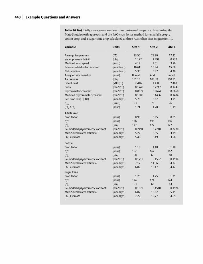
440 Example Questions and Answers
Table 26.7(e) Daily average evaporation from unstressed crops calculated using the
Matt-Shuttleworth approach and the FAO crop factor method for an alfalfa crop, a
cotton crop, and a sugar cane crop calculated at three Australian sites in question 10.
Variable Units Site 1 Site 2 Site 3
Average temperature (°C) 23.50 28.20 17.25Vapor pressure deficit (kPa) 1.177 2.492 0.770Modified wind speed (m s−1) 4.19 3.51 3.70Extraterrestrial solar radiation (mm day−1) 16.61 16.34 15.68Net radiation (mm day−1) 5.35 6.37 4.20Assigned site humidity (none) Humid Arid HumidAir pressure (kPa) 101.16 100.78 100.95Latent heat (MJ kg−1) 2.446 2.434 2.460Delta (kPa °C−1) 0.1740 0.2217 0.1243Psychrometric constant (kPa °C−1) 0.0672 0.0674 0.0668Modified psychrometric constant (kPa °C−1) 0.1600 0.1456 0.1484Ref. Crop Evap. (FAO) (mm day−1) 5.78 8.62 3.75rclim (s m−1) 53 73 76(D50 / D2) (none) 1.21 1.28 1.19
Alfalfa cropCrop factor (none) 0.95 0.95 0.95Rc
50 (none) 196 196 196(rs)c (s/m) 127 127 127Re-modified psychrometric constant (kPa °C−1) 0.2494 0.2210 0.2270Matt-Shuttleworth estimate (mm day−1) 5.22 8.55 3.39FAO estimate (mm day−1) 5.49 8.19 3.56
CottonCrop factor (none) 1.18 1.18 1.18Rc
50 (none) 162 162 162(rs)c (s/m) 60 60 60Re-modified psychrometric constant (kPa °C−1) 0.1713 0.1552 0.1584Matt-Shuttleworth estimate (mm day−1) 7.17 11.36 4.77FAO estimate (mm day−1) 6.82 10.17 4.42
Sugar CaneCrop factor (none) 1.25 1.25 1.25Rc
50 (none) 124 124 124(rs)c (s/m) 63 63 63Re-modified psychrometric constant (kPa °C−1) 0.1673 0.1518 0.1924Matt-Shuttleworth estimate (mm day−1) 6.87 10.82 5.15FAO Estimate (mm day−1) 7.22 10.77 4.69
Shuttleworth_c26.indd 440Shuttleworth_c26.indd 440 11/3/2011 6:38:00 PM11/3/2011 6:38:00 PM