Finance and Economics Discussion SeriesDivisions of Research & Statistics and Monetary Affairs

Federal Reserve Board, Washington, D.C.

Term Structure Modelling with Supply Factors and the FederalReserve’s Large Scale Asset Purchase Programs

Canlin Li and Min Wei

2012-37

NOTE: Staff working papers in the Finance and Economics Discussion Series (FEDS) are preliminarymaterials circulated to stimulate discussion and critical comment. The analysis and conclusions set forthare those of the authors and do not indicate concurrence by other members of the research staff or theBoard of Governors. References in publications to the Finance and Economics Discussion Series (other thanacknowledgement) should be cleared with the author(s) to protect the tentative character of these papers.

Term Structure Modelling with Supply Factors and the Federal

Reserve’s Large Scale Asset Purchase Programs∗

Canlin Li† and Min Wei‡

Preliminary; Comments Welcome

First version: January 20, 2012This version: May 30, 2012

Abstract

This paper proposes and estimates an arbitrage-free term structure model with both ob-

servable yield factors and Treasury and Agency MBS supply factors, and applies it to evaluate

the term premium effects of Federal Reserve’s Large Scale Asset Purchase programs. Our esti-

mates show that the first and the second large-scale asset purchase programs and the Maturity

Extension program have a combined effect of about 100 basis points on the 10-year Treasury

yield.

Keywords: Yield curve, preferred habitat, supply effects, factor models; state-space models;

large-scale asset purchases (LSAP)

JEL Classification: G1, E4, C5

∗The opinions expressed in this paper are those of the authors and do not necessarily reflect views of the FederalReserve Board or the Federal Reserve System. We thank Jim Clouse, Bill English, Thomas Laubach, EmanuelMoench, Fabio Natalucci, Matt Raskin, Tony Rodrigues, and Brian Sack, and participants at the 2012 FRBNYSOMA Portfolio Workshop for helpful comments. All errors are our own.

†Division of Monetary Affairs, Federal Reserve Board of Governors, Canlin.Li@frb.gov, +1-202-452-2227.‡Division of Monetary Affairs, Federal Reserve Board of Governors, Min.Wei@frb.gov, +1-202-736-5619.

1

1 Introduction

Do changes in the supply of Treasury securities and other fixed-income assets affect nominal Trea-

sury yields? This question has received renewed attention as the FOMC adopted large-scale asset

purchases (LSAPs) as an alternative monetary policy tool to stimulate the economy, after the fed-

eral funds rate reached the zero lower bound during the most recent financial crisis. The answer

to this question, however, is still subject to considerable uncertainty. On the one hand, the now-

standard no-arbitrage term structure literature leaves little scope for the relative supply of deeply

liquid financial assets, such as nominal Treasuries, to influence their prices because they can easily

replicated or substituted by other similar assets. On the other hand, there is empirical evidence

suggesting supply effects might exist in the Treasury market. For example, event studies typically

show that the Federal Reserve’s LSAP announcements had nontrivial effects on Treasury yields.

More generally, Krishnamurthy and Vissing-Jorgensen (2008) and Laubach (2009) show that the

total supply of Treasury debt have explanatory power for Treasury yield variations beyond that of

standard yield curve factors, while Hamilton and Wu (Forthcoming) and Greenwood and Vayanos

(2010a,b) provide similar evidence for the maturity structure of Treasury debt outstanding. One

possible explanation for the existence of supply effect in Treasury market is offered by the preferred-

habitat model of interest rates, which assumes imperfect substitutability between securities with

similar maturities.

The preferred-habit literature, which features early contributions by Modigliani and Sutch

(1966, 1967), resorts to the assumption that there exist “preferred-habitat” investors, who demon-

strate preferences for specific maturities, and that interest rate for a given maturity is only in-

fluenced by demand and supply shocks specific to that maturity. Real-world examples of such

preferred-habitat investors include long-term investors, such as pension funds and insurance com-

panies, that prefer to hold long-term bonds to match their long-duration liabilities, and short-term

investors, such as money market mutual funds and foreign reserve managers, that prefer to hold

Treasury bills and short-dated notes to maintain a high degree of liquidity in their portfolio. The

preferred-habitat approach provides a rationale for supply effects in the government bond markets,

as a shock to the stock of privately-held bonds of a particular maturity creates a shortage of those

assets that cannot be wholly relieved, at existing asset prices, by substitution into other securities.

This approach of modeling interest rates has been largely abandoned in today’s term structure

literature, as it implies that yields at different maturities are disconnected from each other, which

is at odds with the continuous yield curve one typically observes. In contrast, in the now-standard

2

arbitrage-free term structure models of Vasicek (1977) and Cox, Jonathan E. Ingersoll, and Ross

(1985), long-term interest rates differ from the expected average future short rate because investors

in long-term bonds demand excess returns for bearing interest rate risks. The existence of ar-

bitrageurs in the economy ensures that the same stochastic discount factor prices interest risks

consistently across the yield curve. It also implies that any changes in the supply of Treasury

securities, if unrelated to the economic fundamentals, should not have significant effect on yields.

More recently, the preferred-habit literature was revitalized in the seminar work of Vayanos and

Vila (2009), who recast Treasury supply and demand shocks in an arbitrage-free framework. In

their model, the existence of preferred-habitat investors provides a channel for demand and supply

factors to influence Treasury yields, while the existence of risk-averse arbitrageurs, who have no

maturity preference but actively trade to take advantage of arbitrage opportunities, ensures that

supply shocks are transmitted smoothly across the yield curve. Vayanos and Vila (2009) show

that, under certain parameterizations, the yield impact of variations in relative supplies depends

on the dollar duration of the supply shocks absorbed by the arbitrageurs, which implies a direct

relationship between the term premium and the total duration risks faced by private investors.

Despite the theoretical advances, empirical studies of preferred-habitat term structure models

are nearly non-existent, hampered by the lack of detailed data on Treasury holdings across investors

and by the complexity of the Vayanos and Vila (2009) model. In this paper, we try to fill this gap

by estimating and testing a no-arbitrage term structure model with supply factors. We adopt

several simplifying assumptions: first, we assume observable supply factors and measure them

using data on private holdings of Treasury debt and agency mortgage backed securities (MBS).

Second, we assume that supply factors influence Treasury yields predominantly through the term

premium channel. Supply affects future short rates only indirectly through current and future term

premiums. Finally, we adopt a two-step estimation approach where factor dynamics are estimated

in the first step while bond risk premium parameters are estimated in the second step.

We also use this model to evaluate the three LSAP programs announced by the Federal Reserve.

Most empirical analysis of the LSAPs are based on either event studies (e.g. Gagnon, Raskin,

Remache, and Sack (2011), Swanson (2011); Krishnamurthy and Vissing-Jorgensen (2011)) or time

series regressions of Treasury yields and/or Treasury term premiums on supply variables (e.g.

Gagnon, Raskin, Remache, and Sack (2011); Greenwood and Vayanos (2010a); Krishnamurthy

and Vissing-Jorgensen (2011); Hamilton and Wu (Forthcoming)). To our knowledge, this paper is

the first to use an arbitrage-free term structure model to evaluate the effects of LSAPs. Results

3

based on event studies are known to be sensitive to the selection of event windows. Time series

regressions used in these studies, on the other hand, are likely susceptible to small-sample bias,

given the highly persistence of supply variables, and endogeneity problems, as changes in Treasury

supply are likely correlated with other factors driving the yield curve. Neither approach can be used

to answer the question of how supply changes affect yields that are not directly used in the study.

By contrast, the no-arbitrage term structure approach in this paper offers a way to consistently

summarize information from the entire yield curve and allows inference across maturities.

Our estimates show that the first and the second large-scale asset purchase programs and the

Maturity Extension program have a combined effect of about 100 basis points on the ten-year

Treasury yield.

While the current paper emphasizes the interest risk premium channel through which LSAP

works to reduce longer term Treasury yields, other channels have been suggested in the literature.

For example, Krishnamurthy and Vissing-Jorgensen (2011) offer evidence that significant clientele

demand exists for long-term “safe” (i.e., nearly default-free) assets, such as Treasury and agency

MBS. These investors are willing to pay a premium—the “safety premium”—for holding those safe

assets. A reduction in the supply of “safe” assets would raise the safety premium and lower the

yields on those assets. Another example is D’Amico and King (2010), who emphasize the scarcity

channel, i.e. a localized effect of supply shocks on yields of nearby maturities. They use CUSIP-

level data to show the Federal Reserve’s purchases have significant yield effects on both purchased

securities and those at nearby maturities.

The remainder of the paper is organized as follows. Section 2 describes the data and documents

the relationship between Treasury term premiums and Treasury and agency MBS supply. Section 3

reviews existing literature on the supply effects in the Treasury market, while Section 4 summarizes

recent studies evaluating the effects of LSAPs on long-term Treasury yields. Section 5 describes

the term structure model with supply factors. Section 6 discusses the estimation methodology and

presents the empirical results. Section 7 concludes.

2 Data and Motivation

This section presents some preliminary evidence suggesting there exists a link between the supply

of government securities and Treasury term premiums.1 In particular, we run monthly regressions

1Hamilton and Wu (Forthcoming) and Greenwood and Vayanos (2010a) also presents evidence on the relationship

between bond supplies and bond risk premiums.

4

of the form

TP 10t = α+ β′SVt + γ′CVt + εt (1)

over the sample period of March 1994 to July 2007, where TP 10t represents estimates of ten-year

Treasury term premium, SVt denotes a vector of supply variables, and CVt denotes a vector of

control variables.

We obtain nominal Treasury yields with maturities of 3, 6, 12, 24, 60, 84, and 120 months from

the Svensson (1995) zero-coupon yield curve maintained by staff at the Federal Reserve Board .2

In this explorative exercise, we use ten-year term premium estimates from a three-latent-factor

Gaussian term structure model developed by Kim and Orphanides (2012), which was estimated

using Treasury yields described above and Blue Chip survey forecasts of 3-month Treasury bill yields

over the next two years and the next five to ten years.3 As discussed in Kim and Orphanides (2012)

and Kim and Wright (2005), incorporating survey forecasts of future short rates helps alleviate

the small sample problem commonly encountered when fitting term structure models to highly

persistent yields.

For reasons that will be discussed later, we include in SVt both Treasury and MBS supply

variables as follows.

• Treasury supply variables, including

– Treasury Par-to-GDP ratio, defined as the par amount of privately-held Treasury secu-

rities as a percentage of nominal GDP, where quarterly data on nominal GDP is taken

from the NIPA account and linearly interpolated to monthly frequency.

– Par-weighted average maturity of privately-held Treasury debt;

– Treasury Ten-year equivalents-to-GDP ratio, defined as the amount of privately-held

Treasury securities (measured in term of ten-year equivalents4) as a percentage of nom-

inal GDP;

• MBS supply variables, including

2Data downloaded from http://www.federalreserve.gov/pubs/feds/2006/200628/200628abs.html. See Gurkaynak,

Sack, and Wright (2007) for details.3Data downloaded from http://www.federalreserve.gov/pubs/feds/2005/200533/200533abs.html.4The ten-year equivalents of a fixed-income portfolio are calculated as the par amount of on-the-run ten-year Trea-

sury notes that would have the same par value times duration as the portfolio under consideration. In mathematical

terms, ten-year equivalents = par value of portfolio * average portfolio duration / duration of the ten-year on-the-run

Treasury note.

5

– MBS par-to-GDP ratio, defined as the par amount of privately-held agency MBS as a

percentage of nominal GDP;

– Par-weighted average duration of privately-held agency MBS;

For each Treasury cusip, the total par amount outstanding as well as the maturity and coupon

rate information are obtained from the Treasury’s Monthly Statement of the Public Debt (MSPD),

while the amount held in the Federal Reserve’s System of Open Market Account (SOMA) is obtained

from the weekly releases by the FRBNY.5 The difference between total debt outstanding and SOMA

holdings gives us the par amount held by private investors for each security. For each Treasury

cusip, we also calculate the average duration and the ten-year equivalents using the same quotes

used in constructing the Svensson yield curve as described above. We then sum over all cusips to

calculate the total par amount and the total ten-year equivalents of private Treasury holdings and

average across cusips to calculate the par amount-weighted average maturity and duration. We

exclude Treasury bills and any previous-issued notes and bonds with remaining maturities below one

year, as commonly done in the literature. For agency MBS, the par amount and average duration

of privately-held agency MBS are taken from Barclays as reported for their MBS index, which

includes mortgage-backed passthrough securities of Ginnie Mae (GNMA), Fannie Mae (FNMA),

and Freddie Mac (FHLMC).

We control for other economic and market factors, CVt, that can be expected to affect term

premiums, including:

• Economic fundamentals, including monthly data on capacity utilization from the Federal

Reserve’s G.17 release and one-year-ahead CPI inflation forecast from Blue Chip Economic

Indicators survey.

• Market volatilities, including implied volatilities from options on ten-year Treasury note fu-

tures and implied volatilities from options on S&P 100 index, both from Bloomberg.

• Foreign demand for Treasury securities, measured by custody holdings of Treasury securities

at the FRBNY on behalf of foreign official and international accounts as a ratio of total Trea-

sury securities outstanding. Data on foreign custody holdings is from the Federal Reserve’s

H.4.1 release.6

5For MSPD, see http://www.treasurydirect.gov/govt/reports/pd/mspd/mspd.htm. For SOMA holdings, see

http://www.newyorkfed.org/markets/soma/sysopen accholdings.html.6See http://www.federalreserve.gov/releases/h41/, memorandum item, ”Marketable securities held in custody for

foreign official and international accounts.”

6

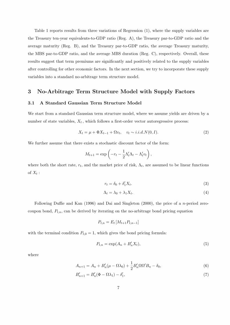
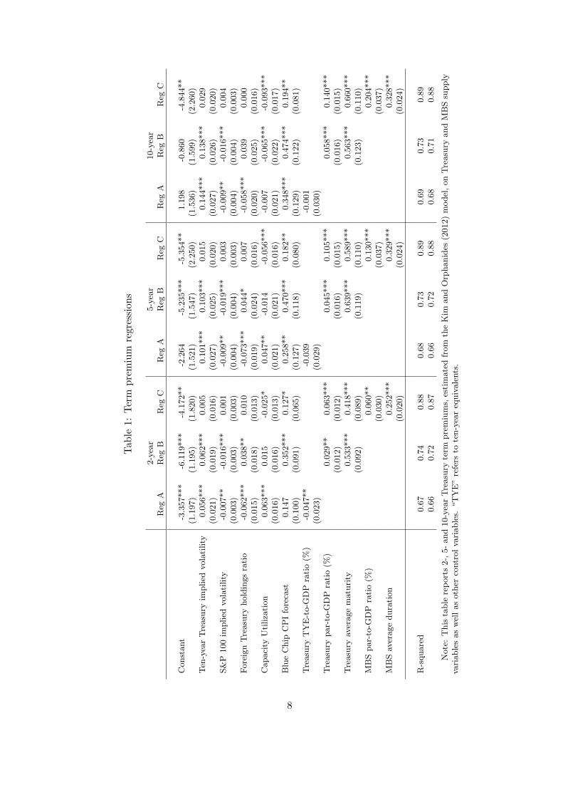
Table 1 reports results from three variations of Regression (1), where the supply variables are

the Treasury ten-year equivalents-to-GDP ratio (Reg. A), the Treasury par-to-GDP ratio and the

average maturity (Reg. B), and the Treasury par-to-GDP ratio, the average Treasury maturity,

the MBS par-to-GDP ratio, and the average MBS duration (Reg. C), respectively. Overall, these

results suggest that term premiums are significantly and positively related to the supply variables

after controlling for other economic factors. In the next section, we try to incorporate these supply

variables into a standard no-arbitrage term structure model.

3 No-Arbitrage Term Structure Model with Supply Factors

3.1 A Standard Gaussian Term Structure Model

We start from a standard Gaussian term structure model, where we assume yields are driven by a

number of state variables, Xt , which follows a first-order vector autoregressive process:

Xt = µ+ΦXt−1 +Ωvt, vt ∼ i.i.d.N(0, I). (2)

We further assume that there exists a stochastic discount factor of the form:

Mt+1 = exp

(−rt −

1

2Λ′tΛt − Λ′

tvt

),

where both the short rate, rt, and the market price of risk, Λt, are assumed to be linear functions

of Xt :

rt = δ0 + δ′1Xt. (3)

Λt = λ0 + λ1Xt. (4)

Following Duffie and Kan (1996) and Dai and Singleton (2000), the price of a n-period zero-

coupon bond, Pt,n, can be derived by iterating on the no-arbitrage bond pricing equation

Pt,n = Et [Mt+1Pt,n−1]

with the terminal condition Pt,0 = 1, which gives the bond pricing formula:

Pt,n = exp(An +B′nXt), (5)

where

An+1 = An +B′n(µ− Ωλ0) +

1

2B′

nΩΩ′Bn − δ0, (6)

B′n+1 = B′

n(Φ− Ωλ1)− δ′1, (7)

7

Tab

le1:

Term

premium

regressions

2-year

5-year

10-year

Reg

AReg

BReg

CReg

AReg

BReg

CReg

AReg

BReg

C

Constant

-3.357***

-6.119***

-4.172**

-2.264

-5.235***

-5.354**

1.198

-0.860

-4.844**

(1.197)

(1.195)

(1.820)

(1.521)

(1.547)

(2.250)

(1.536)

(1.599)

(2.260)

Ten

-yearTreasury

implied

volatility

0.056***

0.062***

0.005

0.101***

0.103***

0.015

0.144***

0.138***

0.029

(0.021)

(0.019)

(0.016)

(0.027)

(0.025)

(0.020)

(0.027)

(0.026)

(0.020)

S&P

100im

plied

volatility

-0.007**

-0.016***

0.001

-0.009**

-0.019***

0.003

-0.009**

-0.016***

0.004

(0.003)

(0.003)

(0.003)

(0.004)

(0.004)

(0.003)

(0.004)

(0.004)

(0.003)

ForeignTreasury

holdingsratio

-0.062***

0.038**

0.010

-0.073***

0.044*

0.007

-0.058***

0.039

0.000

(0.015)

(0.018)

(0.013)

(0.019)

(0.024)

(0.016)

(0.020)

(0.025)

(0.016)

Capacity

Utilization

0.063***

0.015

-0.025*

0.047**

-0.014

-0.056***

-0.007

-0.065***

-0.093***

(0.016)

(0.016)

(0.013)

(0.021)

(0.021)

(0.016)

(0.021)

(0.022)

(0.017)

BlueChip

CPIforecast

0.147

0.352***

0.127*

0.258**

0.470***

0.182**

0.348***

0.474***

0.194**

(0.100)

(0.091)

(0.065)

(0.127)

(0.118)

(0.080)

(0.129)

(0.122)

(0.081)

Treasury

TYE-to-G

DP

ratio(%

)-0.047**

-0.039

-0.001

(0.023)

(0.029)

(0.030)

Treasury

par-to-G

DP

ratio(%

)0.029**

0.063***

0.045***

0.105***

0.058***

0.140***

(0.012)

(0.012)

(0.016)

(0.015)

(0.016)

(0.015)

Treasury

averagematurity

0.533***

0.418***

0.639***

0.589***

0.563***

0.660***

(0.092)

(0.089)

(0.119)

(0.110)

(0.123)

(0.110)

MBSpar-to-G

DP

ratio(%

)0.060**

0.130***

0.204***

(0.030)

(0.037)

(0.037)

MBSav

erageduration

0.252***

0.329***

0.328***

(0.020)

(0.024)

(0.024)

R-squared

0.67

0.74

0.88

0.68

0.73

0.89

0.69

0.73

0.89

0.66

0.72

0.87

0.66

0.72

0.88

0.68

0.71

0.88

Note:Thistable

reports2-,5-and10-yearTreasury

term

premiums,

estimatedfrom

theKim

andOrphanides

(2012)model,onTreasury

andMBSsupply

variablesaswellasother

controlva

riables.

“TYE”refers

toten-yearequivalents.

8

with initial conditions A1 = −δ0 and B1 = −δ1. The bond pricing formula can be rewritten in

yield terms by taking logarithms of both sides of Equation (5)

yt,n = − 1

nlogPt,t+n = − 1

n(An +B′

nXt)

The model can therefore be conveniently represented in a state-space form as follows,

yt,n = − 1

n(An +B′

nXt) + εt,t+n εt,t+n ∼ i.i.d.N(0, σ2n), (8)

Xt = µ+ΦXt−1 +Ωvt vt ∼ i.i.d.N(0, I), (9)

with Equation (8) being the measurement equation and Equation (9) being the state equation.

We consider the risk-neutral measure, under which the state variables follow the process

Xt = µ+ ΦXt−1 + vt,

with the VAR parameters under the physical and the risk-neutral meaures linked to each other

through the relationship

µ = µ− Ωλ0, (10)

Φ = Φ− Ωλ1. (11)

The pricing iterations (6) and (7) can therefore be restated in terms of the risk-neutral VAR

parameters as

An+1 = An +B′nµ+

1

2B′

nΩΩ′Bn − δ0, (12)

B′n+1 = B′

nΦ− δ′1, (13)

while the market price of risk, Λt, can also be written as functions of the two sets of VAR parameters:

Λt = λ0 + λ1Xt = Ω−1[(µ− µ) + (Φ− Φ)Xt)]. (14)

When implementing the model, we directly estimate the physical and risk-neutral VAR parameters,

which jointly decides the market prices of risk.

It is well known at least since Litterman and Scheinkman (1991) that an overwhelming portion

of Treasury yield variations can be summarized by three principal components, frequently termed

the level, the slope and the curvature. In our sample, more than 99% of the yield variations

can be explained by the first two factors, which is the number of yield factors we use in our

empirical analysis. To avoid the difficulty frequently encountered when estimating latent-factor

term structure models, in all our models we assume that these two yield factors are observable and

measure them using the ten-year yield and the spread between the ten-year and the three-month

Treasury yields, respectively.

9

3.2 Term Structure Model with a Treasury Supply Factor

We assume that the state variables, Xt, consist of both yield and supply factors, denoted ft and st,

respectively. The yield factors include the level and slope factors described above. In the first model

we consider, we assume there is only one supply factor, the Treasury ten-year equivalents-to-GDP

ratio.

As in Vayanos and Vila (2009), we motivate our model by assuming the existence of two

types of private participants in the Treasury market: preferred-habitat investors, who hold only a

particular maturity segment of the Treasury yield curve, and risk averse arbitrageurs, who trade to

take advantage of arbitrage opportunities. There are also government agencies, like the Treasury

and the Federal Reserve, which are modeled as risk-neutral participants in the Treasury market.

Vayanos and Vila (2009) show that in how government bond holdings of the arbitragers affect

the equilibrium bond risk premiums. For simplicity, we do not impose specific functional forms

on the demand functions of preferred-habitat investors or the utility function of the arbitrageurs,

which Vayanos and Vila (2009) use to derive analytical solutions linking bond risk premiums to

the arbitragers’ bond holdings. Instead, we simply take their conclusion and assume supply factors

affect bond risk premiums, which is in the same spirit as how macro yield factors are motivated in

the macro-finance term structure models (e.g. Ang and Piazzesi (2003)).

We assume that yield and supply factors only load on their own lags:

Φ =

Φ11 Φ12 0Φ21 Φ22 00 0 Φ33

. (15)

The assumption that yield factors do not load on past supply factors may appear inconsistent with

regression results reported earlier or our stated objective of assessing how supply changes affect

term premium and yields. This assumption is nonetheless imposed to ensure that any evidence we

shall find in support of the supply effects is driven by the data rather than by assumptions. To

ensure that this condition holds empirically, we measure yield factors as residuals from a regression

of the level and the slope of the yield curve on supply factors plus a constant, and order them

first in the VAR. The restriction that supply factors do not load on past yield factors reflects

the Treasury’s stated policy that it “does not ‘time the market’—or seek to take advantage of low

interest rates—when it issues securities. Instead, Treasury strives to lower its borrowing costs over

time by relying on a regular preannounced schedule of auctions.”7

7See http://www.gao.gov/special.pubs/longterm/debt/, which updates information in “Federal Debt: Answers to

Frequently Asked Questions: An Update,” GAO-04-485SP (Washington, D.C.: Aug. 12, 2004).

10

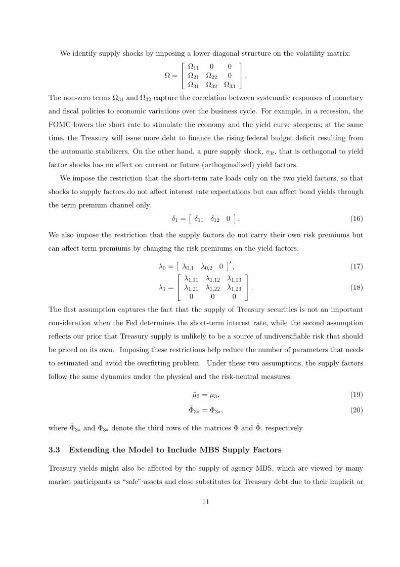
We identify supply shocks by imposing a lower-diagonal structure on the volatility matrix:

Ω =

Ω11 0 0Ω21 Ω22 0Ω31 Ω32 Ω33

,

The non-zero terms Ω31 and Ω32 capture the correlation between systematic responses of monetary

and fiscal policies to economic variations over the business cycle. For example, in a recession, the

FOMC lowers the short rate to stimulate the economy and the yield curve steepens; at the same

time, the Treasury will issue more debt to finance the rising federal budget deficit resulting from

the automatic stabilizers. On the other hand, a pure supply shock, v3t, that is orthogonal to yield

factor shocks has no effect on current or future (orthogonalized) yield factors.

We impose the restriction that the short-term rate loads only on the two yield factors, so that

shocks to supply factors do not affect interest rate expectations but can affect bond yields through

the term premium channel only.

δ1 =[δ11 δ12 0

], (16)

We also impose the restriction that the supply factors do not carry their own risk premiums but

can affect term premiums by changing the risk premiums on the yield factors.

λ0 =[λ0,1 λ0,2 0

]′, (17)

λ1 =

λ1,11 λ1,12 λ1,13

λ1,21 λ1,22 λ1,23

0 0 0

. (18)

The first assumption captures the fact that the supply of Treasury securities is not an important

consideration when the Fed determines the short-term interest rate, while the second assumption

reflects our prior that Treasury supply is unlikely to be a source of undiversifiable risk that should

be priced on its own. Imposing these restrictions help reduce the number of parameters that needs

to estimated and avoid the overfitting problem. Under these two assumptions, the supply factors

follow the same dynamics under the physical and the risk-neutral measures:

µ3 = µ3, (19)

Φ3∗ = Φ3∗, (20)

where Φ3∗ and Φ3∗ denote the third rows of the matrices Φ and Φ, respectively.

3.3 Extending the Model to Include MBS Supply Factors

Treasury yields might also be affected by the supply of agency MBS, which are viewed by many

market participants as “safe” assets and close substitutes for Treasury debt due to their implicit or

11

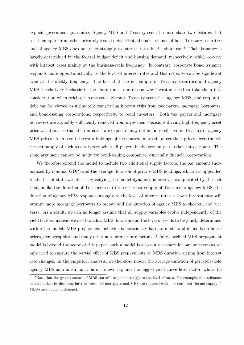
explicit government guarantee. Agency MBS and Treasury securities also share two features that

set them apart from other privately-issued debt. First, the net issuance of both Treasury securities

and of agency MBS does not react strongly to interest rates in the short run.8 Their issuance is

largely determined by the federal budget deficit and housing demand, respectively, which co-vary

with interest rates mainly at the business-cycle frequency. In contrast, corporate bond issuance

responds more opportunistically to the level of interest rates and this response can be significant

even at the weekly frequency. The fact that the net supply of Treasury securities and agency

MBS is relatively inelastic in the short run is one reason why investors need to take them into

consideration when pricing those assets. Second, Treasury securities, agency MBS, and corporate

debt can be viewed as ultimately transferring interest risks from tax payers, mortgage borrowers,

and bond-issuing corporations, respectively, to bond investors. Both tax payers and mortgage

borrowers are arguably sufficiently removed from investment decisions driving high-frequency asset

price variations, so that their interest rate exposure may not be fully reflected in Treasury or agency

MBS prices. As a result, investor holdings of these assets may still affect their prices, even though

the net supply of such assets is zero when all players in the economy are taken into account. The

same argument cannot be made for bond-issuing companies, especially financial corporations.

We therefore extend the model to include two additional supply factors, the par amount (nor-

malized by nominal GDP) and the average duration of private MBS holdings, which are appended

to the list of state variables. Specifying the model dynamics is however complicated by the fact

that, unlike the duration of Treasury securities or the par supply of Treasury or agency MBS, the

duration of agency MBS responds strongly to the level of interest rates; a lower interest rate will

prompt more mortgage borrowers to prepay and the duration of agency MBS to shorten, and vice

versa. As a result, we can no longer assume that all supply variables evolve independently of the

yield factors; instead we need to allow MBS duration and the level of yields to be jointly determined

within the model. MBS prepayment behavior is notoriously hard to model and depends on house

prices, demographics, and many other non-interest rate factors. A fully-specified MBS prepayment

model is beyond the scope of this paper; such a model is also not necessary for our purposes as we

only need to capture the partial effect of MBS prepayments on MBS duration arising from interest

rate changes. In the empirical analysis, we therefore model the average duration of privately-held

agency MBS as a linear function of its own lag and the lagged yield curve level factor, while the

8Note that the gross issuance of MBS can still respond strongly to the level of rates. For example, in a refinance

boom sparked by declining interest rates, old mortgages and MBS are replaced with new ones, but the net supply of

MBS stays about unchanged.

12

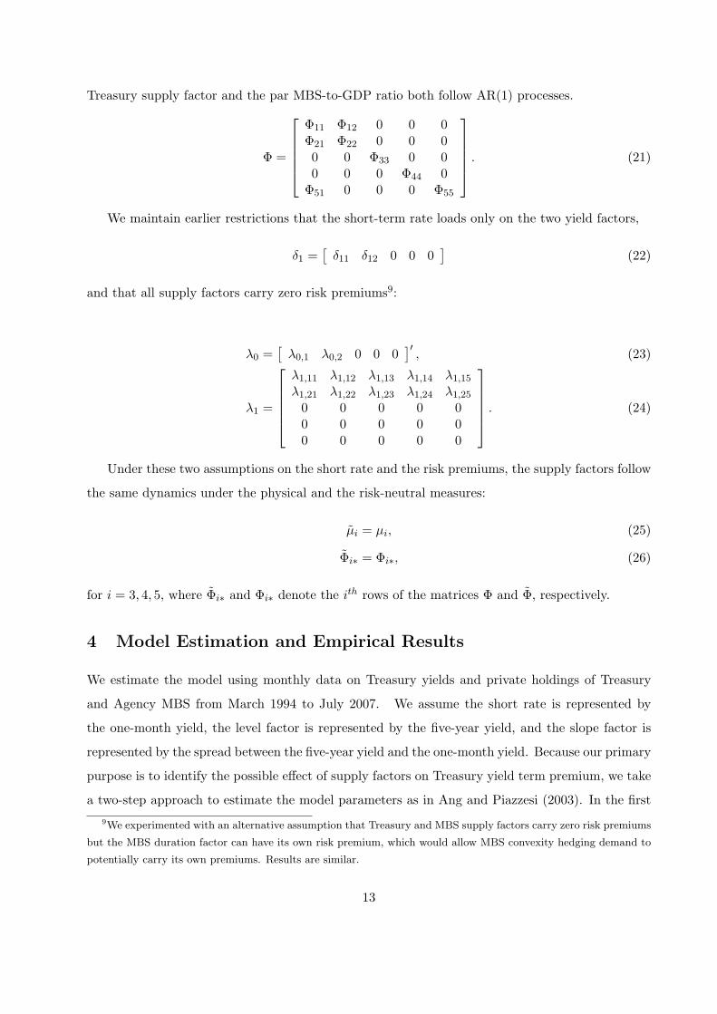
Treasury supply factor and the par MBS-to-GDP ratio both follow AR(1) processes.

Φ =

Φ11 Φ12 0 0 0Φ21 Φ22 0 0 00 0 Φ33 0 00 0 0 Φ44 0

Φ51 0 0 0 Φ55

. (21)

We maintain earlier restrictions that the short-term rate loads only on the two yield factors,

δ1 =[δ11 δ12 0 0 0

](22)

and that all supply factors carry zero risk premiums9:

λ0 =[λ0,1 λ0,2 0 0 0

]′, (23)

λ1 =

λ1,11 λ1,12 λ1,13 λ1,14 λ1,15

λ1,21 λ1,22 λ1,23 λ1,24 λ1,25

0 0 0 0 00 0 0 0 00 0 0 0 0

. (24)

Under these two assumptions on the short rate and the risk premiums, the supply factors follow

the same dynamics under the physical and the risk-neutral measures:

µi = µi, (25)

Φi∗ = Φi∗, (26)

for i = 3, 4, 5, where Φi∗ and Φi∗ denote the ith rows of the matrices Φ and Φ, respectively.

4 Model Estimation and Empirical Results

We estimate the model using monthly data on Treasury yields and private holdings of Treasury

and Agency MBS from March 1994 to July 2007. We assume the short rate is represented by

the one-month yield, the level factor is represented by the five-year yield, and the slope factor is

represented by the spread between the five-year yield and the one-month yield. Because our primary

purpose is to identify the possible effect of supply factors on Treasury yield term premium, we take

a two-step approach to estimate the model parameters as in Ang and Piazzesi (2003). In the first

9We experimented with an alternative assumption that Treasury and MBS supply factors carry zero risk premiums

but the MBS duration factor can have its own risk premium, which would allow MBS convexity hedging demand to

potentially carry its own premiums. Results are similar.

13

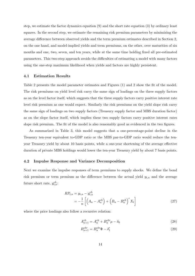
step, we estimate the factor dynamics equation (9) and the short rate equation (3) by ordinary least

squares. In the second step, we estimate the remaining risk premium parameters by minimizing the

average difference between observed yields and the term premium estimates described in Section 2,

on the one hand, and model-implied yields and term premiums, on the other, over maturities of six

months and one, two, seven, and ten years, while at the same time holding fixed all pre-estimated

parameters. This two-step approach avoids the difficulties of estimating a model with many factors

using the one-step maximum likelihood when yields and factors are highly persistent.

4.1 Estimation Results

Table 2 presents the model parameter estimates and Figures (1) and 2 show the fit of the model.

The risk premiums on yield level risk carry the same sign of loadings on the three supply factors

as on the level factor itself, which suggests that the three supply factors carry positive interest rate

level risk premium as one would expect. Similarly the risk premiums on the yield slope risk carry

the same sign of loadings on two supply factors (Treasury supply factor and MBS duration factor)

as on the slope factor itself, which implies these two supply factors carry positive interest rates

slope risk premium. The fit of the model is also reasonably good as evidenced in the two figures.

As summarized in Table 3, this model suggests that a one-percentage-point decline in the

Treasury ten-year equivalent to-GDP ratio or the MBS par-to-GDP ratio would reduce the ten-

year Treasury yield by about 10 basis points, while a one-year shortening of the average effective

duration of private MBS holdings would lower the ten-year Treasury yield by about 7 basis points.

4.2 Impulse Response and Variance Decomposition

Next we examine the impulse responses of term premiums to supply shocks. We define the bond

risk premium or term premium as the difference between the actual yield yt,n and the average

future short rate, yeht,n:

RPt,n = yt,n − yeht,n

= − 1

n

[(An −Aeh

n

)+(Bn −Beh

n

)′Xt

](27)

where the price loadings also follow a recursive relation:

Aehn+1 = Aeh

n +Beh′n µ− δ0 (28)

Beh′n+1 = Beh′

n Φ− δ′1 (29)

14

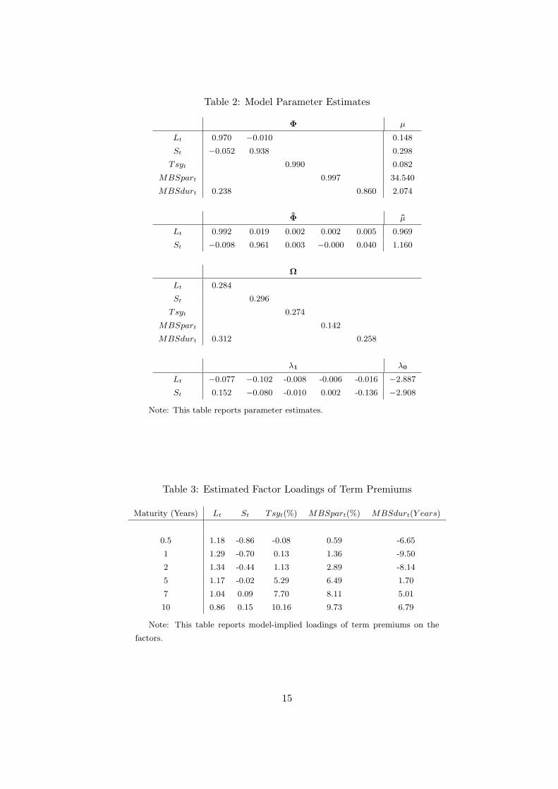
Table 2: Model Parameter Estimates

Φ µ

Lt 0.970 −0.010 0.148

St −0.052 0.938 0.298

Tsyt 0.990 0.082

MBSpart 0.997 34.540

MBSdurt 0.238 0.860 2.074

Φ µ

Lt 0.992 0.019 0.002 0.002 0.005 0.969

St −0.098 0.961 0.003 −0.000 0.040 1.160

Ω

Lt 0.284

St 0.296

Tsyt 0.274

MBSpart 0.142

MBSdurt 0.312 0.258

λ1 λ0

Lt −0.077 −0.102 -0.008 -0.006 -0.016 −2.887

St 0.152 −0.080 -0.010 0.002 -0.136 −2.908

Note: This table reports parameter estimates.

Table 3: Estimated Factor Loadings of Term Premiums

Maturity (Years) Lt St Tsyt(%) MBSpart(%) MBSdurt(Y ears)

0.5 1.18 -0.86 -0.08 0.59 -6.65

1 1.29 -0.70 0.13 1.36 -9.50

2 1.34 -0.44 1.13 2.89 -8.14

5 1.17 -0.02 5.29 6.49 1.70

7 1.04 0.09 7.70 8.11 5.01

10 0.86 0.15 10.16 9.73 6.79

Note: This table reports model-implied loadings of term premiums on the

factors.

15

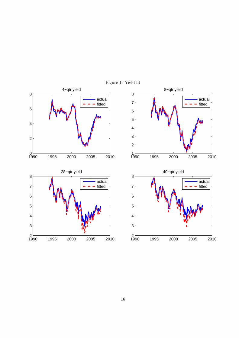
Figure 1: Yield fit

1990 1995 2000 2005 20100

2

4

6

84−qtr yield

actualfitted

1990 1995 2000 2005 20101

2

3

4

5

6

7

88−qtr yield

actualfitted

1990 1995 2000 2005 20102

3

4

5

6

7

828−qtr yield

actualfitted

1990 1995 2000 2005 20102

3

4

5

6

7

840−qtr yield

actualfitted

16

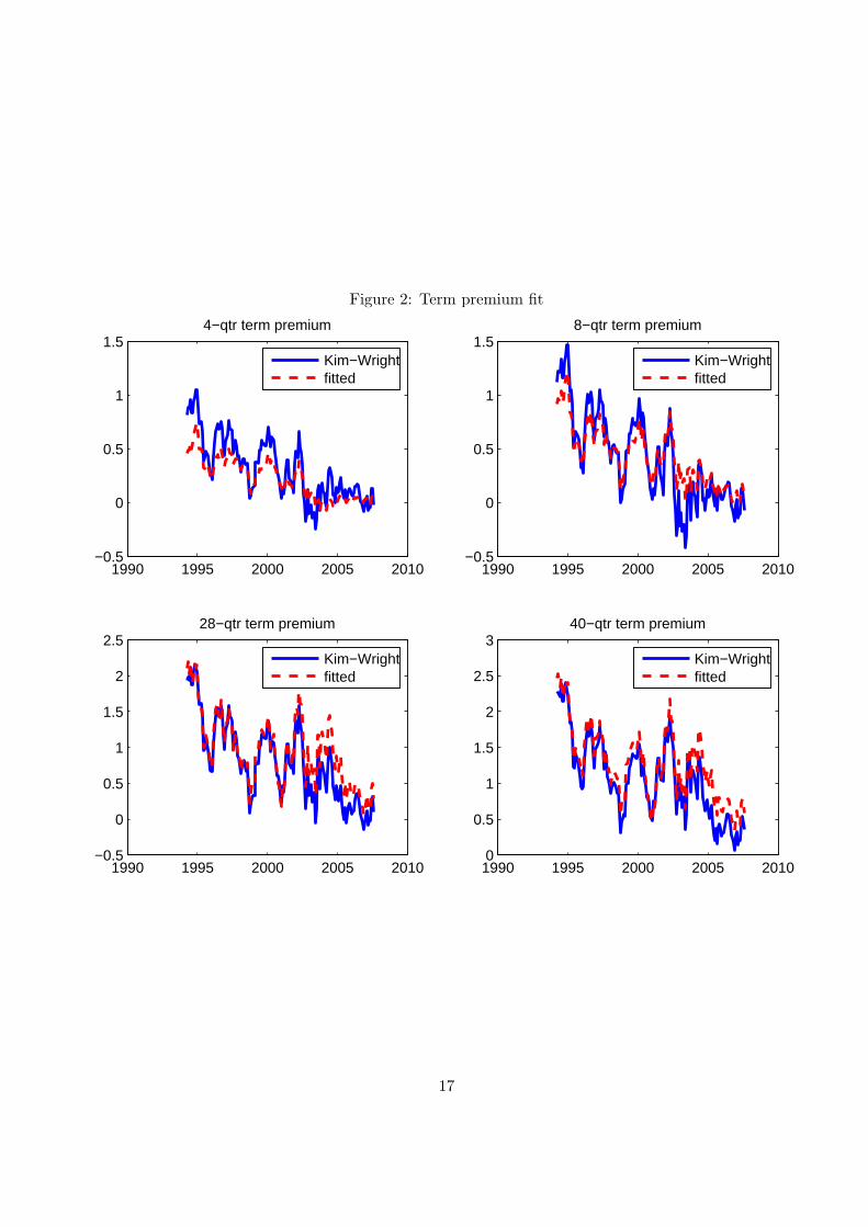
Figure 2: Term premium fit

1990 1995 2000 2005 2010−0.5

0

0.5

1

1.54−qtr term premium

Kim−Wrightfitted

1990 1995 2000 2005 2010−0.5

0

0.5

1

1.58−qtr term premium

Kim−Wrightfitted

1990 1995 2000 2005 2010−0.5

0

0.5

1

1.5

2

2.528−qtr term premium

Kim−Wrightfitted

1990 1995 2000 2005 20100

0.5

1

1.5

2

2.5

340−qtr term premium

Kim−Wrightfitted

17

with the initial conditions Aeh1 = A1 = −δ0 and Beh

1 = B1 = −δ1. Note that in our setup, the

average future short rate only loads on yield factors. We can therefore focus exclusively on the

term premium components of yields in our analysis of the effects of supply variables on the term

structure.

Recall there are only two risk factors in this model, i.e., only the first two elements in the

price of risk vector, Λt = λ0 + λ1Xt, are non-zeros. The top panel of Figure 3 plots the impulse

responses of these two elements, which represent the market price of yield curve level and slope

risks, respectively, to one unit of shock to each supply factor. The market price of yield slope

risk seems to react more strongly to MBS duration shocks than the price of level risk, while the

responses to Treasury and MBS par supply factors are comparable across the two prices of risk.

Turning to term premiums, the bottom panel of Figure 3 plots impulse responses of 5-year and

10-year term premiums to one unit of shock to each supply factor as implied by Equations (2) and

(27). MBS duration shocks seem to have smaller and more transitory effects on yields than the

other two shocks, while the effects of Treasury and MBS par supply factors are both long-lasting

and rising with bond maturities.

We can also use Equations (2) and (27) to decompose the conditional variance V art(RPt+h,n)

at horizon h and maturity n as explained by each factor. The results for maturities of 1, 5, 10 years

and horizons of 12 and 60 months are reported in Figure 4 and Table 4. As expected, the Treasury

and MBS par supply factors explain very little of term premium variations at short maturities and

short horizons, because short-term yields are primarily driven by interest rate expectations, which

by construction are not affected by supply factors; in addition, supply factors are highly persistent

and show little variations over short horizons. As the maturity rises, however, changes in term

premiums explain a larger portion of yield variations. As the forecasts horizon increases, supply

factors also exhibit more notable variations. Taken together, these two observations suggest that

the effect of supply factors on term premiums should become more important at longer maturities

and horizons, which is what we observe in the data. More specifically, about 9% and 20% of the

conditional variance of 5- and 10-year term premiums, respectively, are attributable to shocks to

the supply factors. Moreover, the Treasury supply factor accounts for most of the contributions of

supply factors to term premium variations.

18

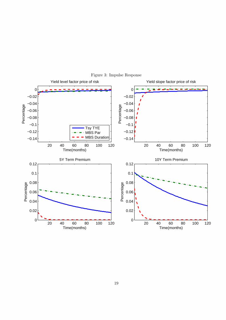
Figure 3: Impulse Response

20 40 60 80 100 120

−0.14

−0.12

−0.1

−0.08

−0.06

−0.04

−0.02

0

Time(months)

Per

cent

age

Yield level factor price of risk

Tsy TYEMBS ParMBS Duration

20 40 60 80 100 120

−0.14

−0.12

−0.1

−0.08

−0.06

−0.04

−0.02

0

Time(months)

Per

cent

age

Yield slope factor price of risk

20 40 60 80 100 1200

0.02

0.04

0.06

0.08

0.1

0.12

Time(months)

Per

cent

age

5Y Term Premium

20 40 60 80 100 1200

0.02

0.04

0.06

0.08

0.1

0.12

Time(months)

Per

cent

age

10Y Term Premium

19

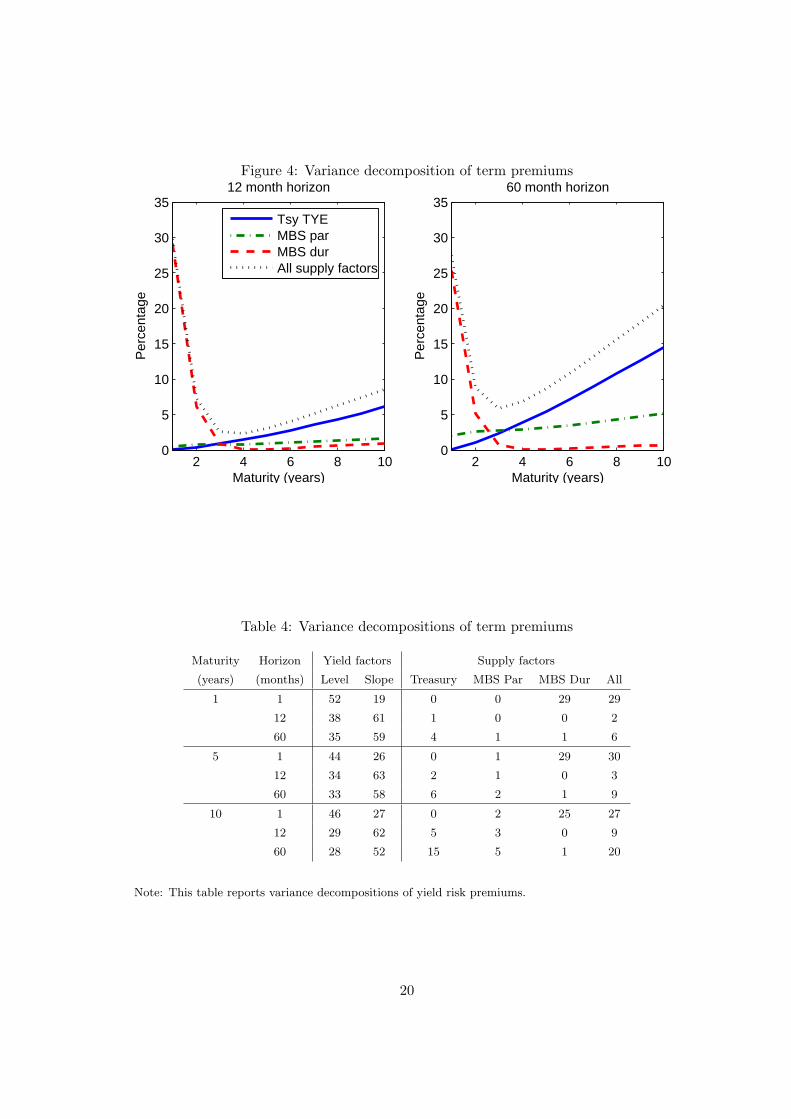
Figure 4: Variance decomposition of term premiums

2 4 6 8 100

5

10

15

20

25

30

35

Maturity (years)

Per

cent

age

12 month horizon

Tsy TYEMBS parMBS durAll supply factors

2 4 6 8 100

5

10

15

20

25

30

35

Maturity (years)

Per

cent

age

60 month horizon

Table 4: Variance decompositions of term premiums

Maturity Horizon Yield factors Supply factors

(years) (months) Level Slope Treasury MBS Par MBS Dur All

1 1 52 19 0 0 29 29

12 38 61 1 0 0 2

60 35 59 4 1 1 6

5 1 44 26 0 1 29 30

12 34 63 2 1 0 3

60 33 58 6 2 1 9

10 1 46 27 0 2 25 27

12 29 62 5 3 0 9

60 28 52 15 5 1 20

Note: This table reports variance decompositions of yield risk premiums.

20

5 Evaluating the Federal Reserve’s Asset Purchase Programs

This section uses our term structure model with supply factors to evaluate the Federal Reserve’s

previous asset purchase programs—LSAP1, LSAP2, and MEP, which provide natural experiments

for assessing the effects of exogenous shocks to the supply of Treasury securities and their close

substitutes on Treasury yields. For reference, the details of these programs are described briefly

below.10

• LSAP1: On November 25, 2008, the FOMC announced the first LSAP program (LSAP1)

consisting of $100 billion of purchases of agency debt and up to $500 billion of purchases

of agency MBS. In March 2009, the FOMC expanded the LSAP1 program to include an

additional $750 billion purchase of agency securities and $300 billion purchase of longer-term

Treasury securities. The program was completed in March 2010, with a total purchase of

$1.25 trillion of agency MBS, about $170 billion of agency debt, and $300 billion of Treasury

securities.

• LSAP2: On November 3, 2010, the FOMC announced it would purchase $600 billion of

longer-term Treasury securities over an 8-month period through June 2011 (LSAP2). LSAP2

was completed as announced, with the bulk of purchases concentrated in nominal Treasury

securities with 2- to 10-year maturities.

• MEP: On September 21, 2011, the FOMC announced the Maturity Extension Program

(MEP), under which the FOMC will purchase, by the end of June 2012, $400 billion of

Treasury securities with remaining maturities of 6 to 30 years while simultaneously selling

an equal amount of Treasuries with remaining maturities of 3 years or less. Staff estimates

suggest that both the LSAP2 program and the MEP would remove about $400 billion of

10-year equivalents of private Treasury holdings from the market.

10There were also two changes in how principal payments from SOMA holdings of agency debt and agency MBS

are handled. Those principal payments were allowed to roll off the Federal Reserve’s balance sheet from the start

of the LSAP1 program till August 2010, when they were reinvested in longer-term Treasury securities instead. The

current policy of reinvesting those principal payments in agency MBS was announced in September 2011, together

with the MEP. The first reinvestment policy change was taken into account in our analysis of the LSAP2 program

but not the LSAP1 program, while the second reinvestment policy change was taken into account in our analysis of

the MEP but not the LSAP1 or the LSAP2 programs.

21

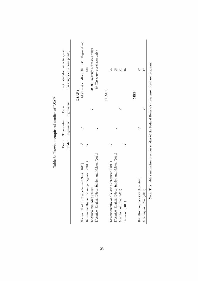
5.1 Previous empirical studies

A growing empirical literature tries to assess the effects of these asset purchase programs, which

are summarized in Table 5 and described in more details below.

LSAP1

1. Gagnon, Raskin, Remache, and Sack (2011) using one-day window around 8 baseline events

from November 25, 2008 to November 4, 2009, find that the 2-year Treasury yield declined

34bps , the ten-year Treasury yield declined 91bps, the ten-year agency debt yield declined

156bps, the current-coupon 30-year MBS yield declined 113bps, the ten-year SWAP rate

101bps, and the Baa corporate bond index yield declined 67 bps. Gagnon, Raskin, Remache,

and Sack (2011) also use several regression models on a sample from January 1985 to June

2008, to estimate the effect of changes in the stock of privately-held longer-term debt (nor-

malized by nominal GDP) on the term premium, after controlling for other factors related

to business cycles, and uncertainties about economic fundamentals. From those regression

models they estimate the term premium effects of the first LSAP are 36 to 82bps.

2. D’Amico and King (2010), which focuses only on Treasury LSAPs, using a panel of CUSIP-

level data (where they regress the cumulative change in each security price on the total amount

purchased of that security and its close substitutes) find that at the end of the first LSAP,

Treasury yields with remaining maturity between 5 to 15 years were 20 to 30 basis points

lower than what they would otherwise have been. The largest effects are at horizons of about

6 to 8 years and 11 to 14 years, consistent with the relatively high proportion of securities

purchased in these sectors.

3. D’Amico, English, Lopez-Salido, and Nelson (2011) provide empirical estimates of the effect

on longer-term U.S. Treasury yields of LSAP-style operations focusing on two channels: (i)

scarcity (available local supply) and (ii) duration. According to these estimates the total

impact from the first Treasury LSAP program is about 35 basis points: the scarcity effect

accounts for 23 basis points and the duration effect for 12 basis points. The estimates indicate

that: both proxies for scarcity and duration are positively and significantly related to longer-

term Treasury yields and term premiums; a sizable portion of the impact on longer-term

Treasury yields has been transmitted via the nominal term-premium component; within the

overall term premium, it is the real term premium component that exhibits the greatest

response to these two variables; and the inflation risk premium’s response, in contrast, is

22

Tab

le5:

Previousem

piricalstudiesofLSAPs

Event

Tim

eseries

Panel

Estim

ateddeclinein

ten-year

studies

regressions

regressions

Treasury

yield

(basispoints)

LSAP1

Gagnon,Raskin,Rem

ach

e,andSack

(2011)

XX

91(E

ven

tstudies);36to

82(R

egressions)

KrishnamurthyandVissing-Jorgen

sen(2011)

X100

D’A

micoandKing(2010)

X20-30(T

reasury

purchasesonly)

D’A

mico,English,Lopez-Salido,andNelson(2011)

X35(T

reasury

purchasesonly)

LSAP2

KrishnamurthyandVissing-Jorgen

sen(2011)

X25

D’A

mico,English,Lopez-Salido,andNelson(2011)

X55

MeaningandZhu(2011)

X21

Swanson(2011)

X15

MEP

HamiltonandWu(Forthcoming)

X22

MeaningandZhu(2011)

X17

Note:This

table

summarizespreviousstudiesoftheFed

eralReserve’sthreeasset

purchase

programs.

23

quite small and is not uniformly statistically significant across different specifications.

4. Krishnamurthy and Vissing-Jorgensen (2011) using one-day window around 6 baseline events

from November 25, 2008 to March 18, 2009, find that the ten-year Treasury yield declined

100bps, the ten-year agency debt yield declined 164bps, the current-coupon 30-year MBS

yield declined 116bps, and the Baa corporate bond index yield declined 68bps.

Overall, the above mentioned studies imply that the first round of Treasury LSAPs had an

impact that ranges between 15 and 35 basis points.

LSAP2

1. Krishnamurthy and Vissing-Jorgensen (2011) using an event-study approach that analyzes

the period from August 26, 2010 (day before the Chairman Bernanke’s Jackson Hole speech)

to November 2, 2010 (day before the LSAP2 announcement), find that the ten-year Treasury

yield declined 25bps, the ten-year agency debt yield declined 27bps, and the Baa corporate

bond index yield declined 17bps. In addition, their regression approach predicts that LSAP2

should result in a 26.5 basis-point decline in Treasury yields, which is quite aligned with the

event-study results.

2. D’Amico, English, Lopez-Salido, and Nelson (2011) results suggest that the scarcity effect

from the second LSAP program is about 45 basis points and the duration effect is about 10

basis points. Thus, the total effect of the second LSAP is estimated to be about 55 basis

points.

3. Meaning and Zhu (2011) applying the methodology developed by D’Amico and King (2010)

estimate that LSAP2 on average lowered the yield curve by 21 basis points, with a maximum

impact of 108 basis point for some securities with remaining maturity of about 20 years.

4. Swanson (2011) also employs an event-study approach to measure the impact of Operation

Twist (1961) that is extrapolated to quantify the effect of LSAP2, based on similarities

between the two programs. The size of Operation Twist accounted for 4.5% of U.S. Treasury-

guaranteed debt and it appeared to have reduced short- and long-term rates by 13bps. The

size of LSAP2 was very similar to Operation Twist as percentage of Treasury debt, and it is

estimated to have reduced long-term rates by 15bps.

MEP

24

1. Meaning and Zhu (2011) simulations suggest that on average, yields may drop 22 basis points

for securities with a remaining maturity over 8 years.

2. Hamilton and Wu (Forthcoming), using regression on a sample from 1990 to 2007, estimate

the effect of variations in the average maturity of privately-held Treasury debt on the term

structure of interest rates, after controlling for level, slope and curvature of the yield curve.

Using the estimated coefficients they evaluate a swap experiment where the Fed sells $400bn

of short-term securities and buys $400bn of long-term securities. The results indicate that

yields with maturity longer than 2 year fall about 17 basis points, while short-term yields

increase of a similar amount.

5.2 LSAPs as One-Period Supply Shocks

Most studies mentioned above treated these asset purchase programs as causing instant shocks

to the supply variables. Following the same approach, we consider the $300 billion of Treasury

security purchase in LSAP1 as roughly corresponding to a $169 billion shock to private Treasury

holdings in terms of ten-year equivalents (Gagnon, Raskin, Remache, and Sack (2011), footnote 47),

or a 1.2 percent shock to the Treasury supply factor when normalized by the 2009Q4 nominal GDP

of $14.1 trillion. Similarly, the $1.25 trillion purchases of Agency MBS under the LSAP1 program

roughly translates into a 8.9 percent shock to the MBS par supply factor. By comparison, both

the $600 billion of Treasury Purchase under the LSAP2 program and the $400 billion simultaneous

purchases of Treasury security with maturities longer than 6 years and sales of Treasury securities

with maturity less than 3 years under the MEP are estimated to have removed about $400 billion

10-equivalents from the market, or about 2.6 percent and 2.5 percent shocks to the Treasury supply

factor when normalized by the 2010Q4 and the 2011Q4 nominal GDP of $14.7 trillion and $15.3

trillion, respectively.

We use the estimated factor loadings in Table 3 to estimate the term premium effects of such

supply shocks and summarize the results in Table 6. We estimate that the LSAP1 program lowered

the ten-year Treasury yield by about 100 basis points, the five-year yield by about 65 basis points,

and the two-year yield by about 25 basis points in the near term. By comparison, the other two

programs (the LSAP2 program and the MEP) are both estimated to have lowered the ten-year

Treasury yield by about 25 basis points and the five-year yield by 10 to 15 basis points, but have

almost no effect on the two-year Treasury yield.

25

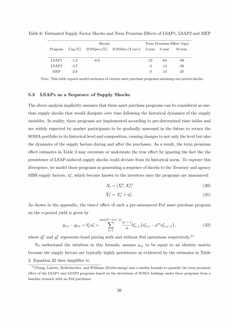
Table 6: Estimated Supply Factor Shocks and Term Premium Effects of LSAP1, LSAP2 and MEP

Shocks Term Premium Effect (bps)

Program Tsyt(%) MBSpart(%) MBSdurt(Y ears) 2-year 5-year 10-year

LSAP1 -1.2 -8.9 -27 -64 -99

LSAP2 -2.7 -3 -14 -26

MEP -2.6 -3 -13 -25

Note: This table reports model estimates of various asset purchase programs assuming one-period shocks.

5.3 LSAPs as a Sequence of Supply Shocks

The above analysis implicitly assumes that these asset purchase programs can be considered as one-

time supply shocks that would dissipate over time following the historical dynamics of the supply

variables. In reality, these programs are implemented according to pre-determined time tables and

are widely expected by market participants to be gradually unwound in the future to return the

SOMA portfolio to its historical level and composition, causing changes to not only the level but also

the dynamics of the supply factors during and after the purchases. As a result, the term premium

effect estimates in Table 3 may overstate or understate the true effect by ignoring the fact the the

persistence of LSAP-induced supply shocks could deviate from its historical norm. To capture this

divergence, we model those programs as generating a sequence of shocks to the Treasury and agency

MBS supply factors, ust , which become known to the investors once the programs are announced:

Xt = [Xyt , X

st ]

′ (30)

Xst = Xs

t + ust , (31)

As shown in the appendix, the time-t effect of such a pre-announced Fed asset purchase program

on the n-period yield is given by

yt,n − yt,n = bsnust +

minT−t,n−1∑i=1

n− i

nbsn−i

(ust+i − ρssust+i−1

), (32)

where ynt and ynt represents bond pricing with and without Fed operations respectively.11

To understand the intuition in this formula, assume ρss to be equal to an identity matrix

because the supply factors are typically highly persistence as evidenced by the estimates in Table

2. Equation 32 then simplifies to

11Chung, Laforte, Reifschneider, and Williams (Forthcoming) uses a similar formula to quantify the term premium

effect of the LSAP1 and LSAP2 programs based on the deviations of SOMA holdings under these programs from a

baseline scenario with no Fed purchases.

26

yt,n − yt,n = bsnust +

minT−t,n−1∑i=1

n− i

nbsn−i

(ust+i − ust+i−1

), (33)

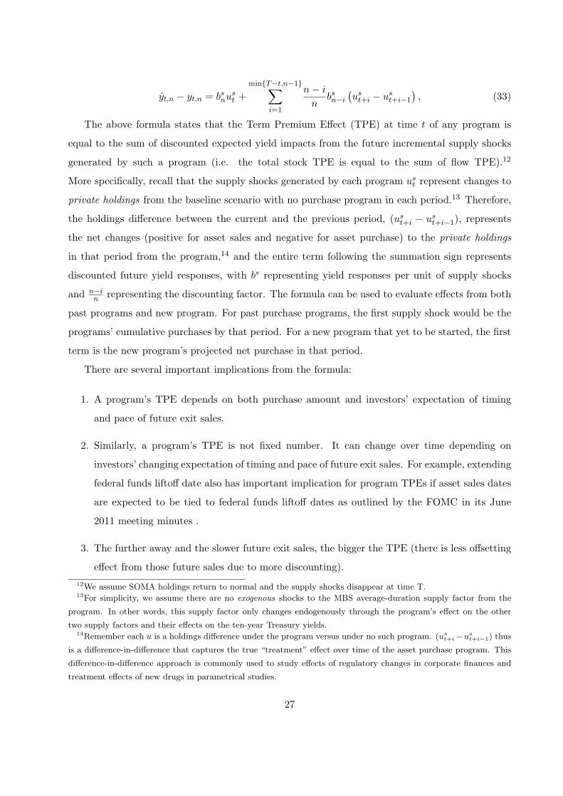
The above formula states that the Term Premium Effect (TPE) at time t of any program is

equal to the sum of discounted expected yield impacts from the future incremental supply shocks

generated by such a program (i.e. the total stock TPE is equal to the sum of flow TPE).12

More specifically, recall that the supply shocks generated by each program ust represent changes to

private holdings from the baseline scenario with no purchase program in each period.13 Therefore,

the holdings difference between the current and the previous period, (ust+i − ust+i−1), represents

the net changes (positive for asset sales and negative for asset purchase) to the private holdings

in that period from the program,14 and the entire term following the summation sign represents

discounted future yield responses, with bs representing yield responses per unit of supply shocks

and n−in representing the discounting factor. The formula can be used to evaluate effects from both

past programs and new program. For past purchase programs, the first supply shock would be the

programs’ cumulative purchases by that period. For a new program that yet to be started, the first

term is the new program’s projected net purchase in that period.

There are several important implications from the formula:

1. A program’s TPE depends on both purchase amount and investors’ expectation of timing

and pace of future exit sales.

2. Similarly, a program’s TPE is not fixed number. It can change over time depending on

investors’ changing expectation of timing and pace of future exit sales. For example, extending

federal funds liftoff date also has important implication for program TPEs if asset sales dates

are expected to be tied to federal funds liftoff dates as outlined by the FOMC in its June

2011 meeting minutes .

3. The further away and the slower future exit sales, the bigger the TPE (there is less offsetting

effect from those future sales due to more discounting).

12We assume SOMA holdings return to normal and the supply shocks disappear at time T.13For simplicity, we assume there are no exogenous shocks to the MBS average-duration supply factor from the

program. In other words, this supply factor only changes endogenously through the program’s effect on the other

two supply factors and their effects on the ten-year Treasury yields.14Remember each u is a holdings difference under the program versus under no such program. (us

t+i−ust+i−1) thus

is a difference-in-difference that captures the true “treatment” effect over time of the asset purchase program. This

difference-in-difference approach is commonly used to study effects of regulatory changes in corporate finances and

treatment effects of new drugs in parametrical studies.

27

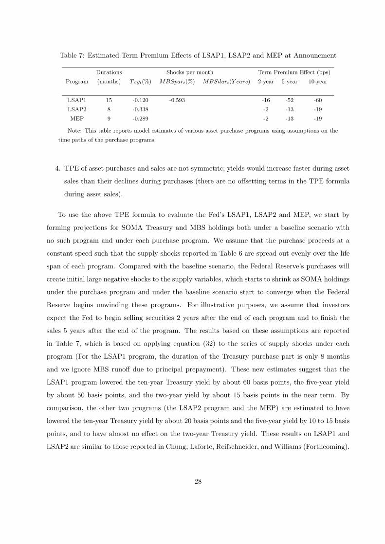
Table 7: Estimated Term Premium Effects of LSAP1, LSAP2 and MEP at Announcment

Durations Shocks per month Term Premium Effect (bps)

Program (months) Tsyt(%) MBSpart(%) MBSdurt(Y ears) 2-year 5-year 10-year

LSAP1 15 -0.120 -0.593 -16 -52 -60

LSAP2 8 -0.338 -2 -13 -19

MEP 9 -0.289 -2 -13 -19

Note: This table reports model estimates of various asset purchase programs using assumptions on the

time paths of the purchase programs.

4. TPE of asset purchases and sales are not symmetric; yields would increase faster during asset

sales than their declines during purchases (there are no offsetting terms in the TPE formula

during asset sales).

To use the above TPE formula to evaluate the Fed’s LSAP1, LSAP2 and MEP, we start by

forming projections for SOMA Treasury and MBS holdings both under a baseline scenario with

no such program and under each purchase program. We assume that the purchase proceeds at a

constant speed such that the supply shocks reported in Table 6 are spread out evenly over the life

span of each program. Compared with the baseline scenario, the Federal Reserve’s purchases will

create initial large negative shocks to the supply variables, which starts to shrink as SOMA holdings

under the purchase program and under the baseline scenario start to converge when the Federal

Reserve begins unwinding these programs. For illustrative purposes, we assume that investors

expect the Fed to begin selling securities 2 years after the end of each program and to finish the

sales 5 years after the end of the program. The results based on these assumptions are reported

in Table 7, which is based on applying equation (32) to the series of supply shocks under each

program (For the LSAP1 program, the duration of the Treasury purchase part is only 8 months

and we ignore MBS runoff due to principal prepayment). These new estimates suggest that the

LSAP1 program lowered the ten-year Treasury yield by about 60 basis points, the five-year yield

by about 50 basis points, and the two-year yield by about 15 basis points in the near term. By

comparison, the other two programs (the LSAP2 program and the MEP) are estimated to have

lowered the ten-year Treasury yield by about 20 basis points and the five-year yield by 10 to 15 basis

points, and to have almost no effect on the two-year Treasury yield. These results on LSAP1 and

LSAP2 are similar to those reported in Chung, Laforte, Reifschneider, and Williams (Forthcoming).

28

6 Conclusions

In this paper, we provide evidence that private holdings of Treasury securities and agency MBS

have explanatory power for variations in Treasury yields above and beyond that of standard yield

curve factors.

Based on this observation, we extend the standard Gaussian essentially affine no-arbitrage term

structure model to allow Treasury and MBS supply variables to affect Treasury term premiums.

The model is fitted to historical data on Treasury yields as well as the supply and the maturity

characteristics of private Treasury and MBS holdings. The estimation results suggest that a one-

percentage-point decline in the Treasury ten-year equivalent to GDP ratio or the MBS par-to-GDP

ratio would reduce the ten-year Treasury yield by about 10 basis points, while a one-year shortening

of the average effective duration of private MBS holdings would lower the ten-year Treasury yield

by about 7 basis points.

We then apply this model to evaluating the Federal Reserve’s various asset purchase programs.

Our estimates show that the first and the second large-scale asset purchase programs and the

Maturity Extension program have a combined effect of about 100 basis points on the ten-year

Treasury yield.

29

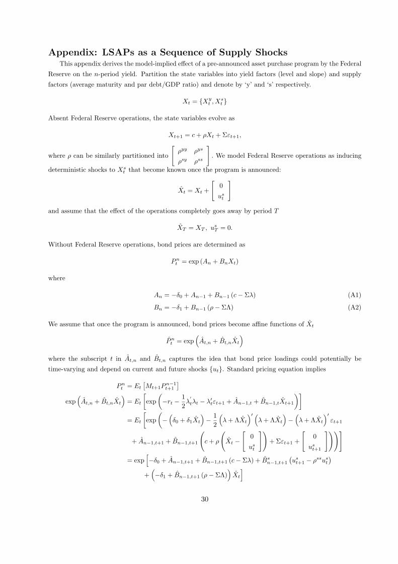
Appendix: LSAPs as a Sequence of Supply ShocksThis appendix derives the model-implied effect of a pre-announced asset purchase program by the Federal

Reserve on the n-period yield. Partition the state variables into yield factors (level and slope) and supply

factors (average maturity and par debt/GDP ratio) and denote by ‘y’ and ‘s’ respectively.

Xt = Xyt , X

st

Absent Federal Reserve operations, the state variables evolve as

Xt+1 = c+ ρXt +Σεt+1,

where ρ can be similarly partitioned into

[ρyy ρys

ρsy ρss

]. We model Federal Reserve operations as inducing

deterministic shocks to Xst that become known once the program is announced:

Xt = Xt +

[0

ust

]

and assume that the effect of the operations completely goes away by period T

XT = XT , usT = 0.

Without Federal Reserve operations, bond prices are determined as

Pnt = exp (An +BnXt)

where

An = −δ0 +An−1 +Bn−1 (c− Σλ) (A1)

Bn = −δ1 +Bn−1 (ρ− ΣΛ) (A2)

We assume that once the program is announced, bond prices become affine functions of Xt

Pnt = exp

(At,n + Bt,nXt

)where the subscript t in At,n and Bt,n captures the idea that bond price loadings could potentially be

time-varying and depend on current and future shocks ut. Standard pricing equation implies

Pnt = Et

[Mt+1P

n−1t+1

]exp

(At,n + Bt,nXt

)= Et

[exp

(−rt −

1

2λ

′

tλt − λ′tεt+1 + An−1,t + Bn−1,tXt+1

)]= Et

[exp

(−(δ0 + δ1Xt

)− 1

2

(λ+ ΛXt

)′ (λ+ ΛXt

)−(λ+ ΛXt

)′εt+1

+ An−1,t+1 + Bn−1,t+1

(c+ ρ

(Xt −

[0

ust

])+Σεt+1 +

[0

ust+1

]))]= exp

[−δ0 + An−1,t+1 + Bn−1,t+1 (c− Σλ) + Bs

n−1,t+1

(ust+1 − ρssus

t

)+(−δ1 + Bn−1,t+1 (ρ− ΣΛ)

)Xt

]

30

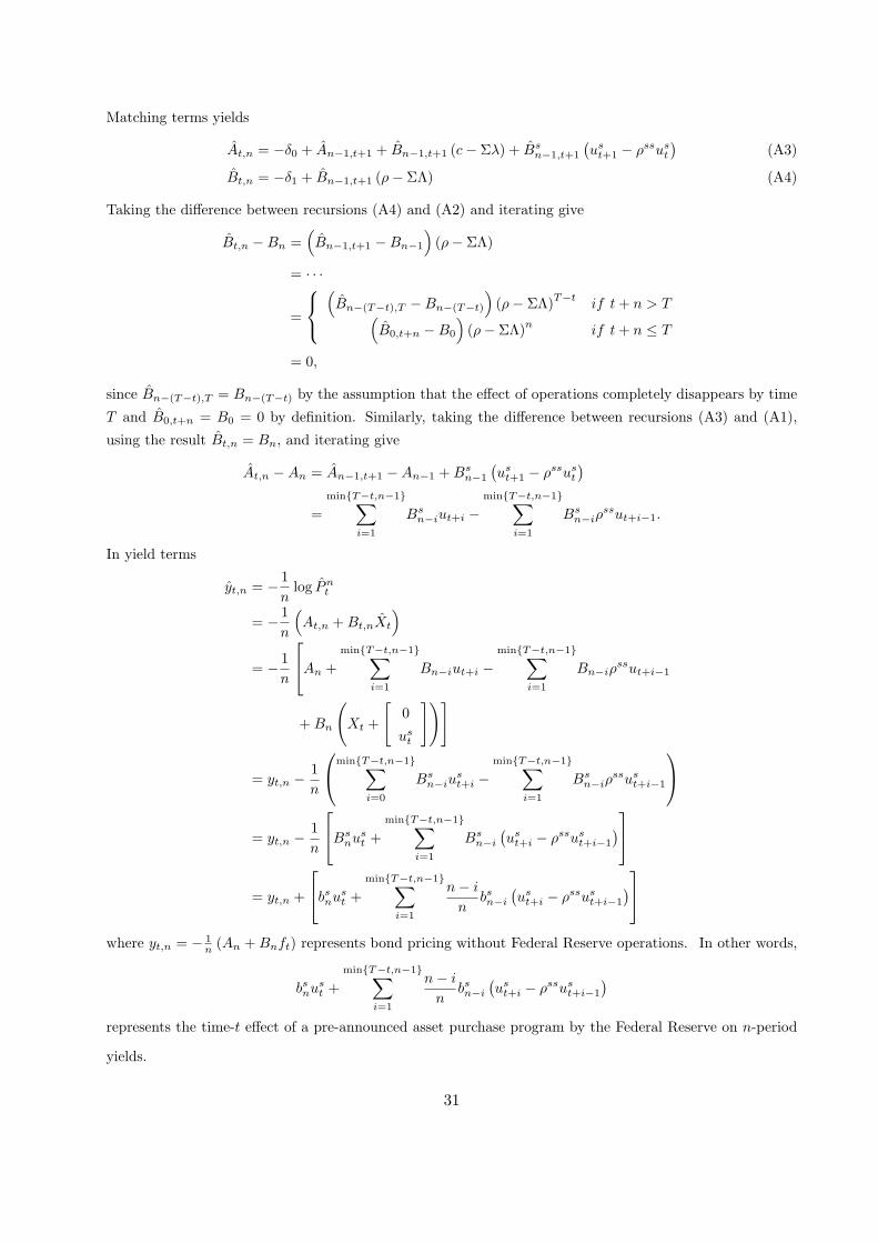
Matching terms yields

At,n = −δ0 + An−1,t+1 + Bn−1,t+1 (c− Σλ) + Bsn−1,t+1

(ust+1 − ρssus

t

)(A3)

Bt,n = −δ1 + Bn−1,t+1 (ρ− ΣΛ) (A4)

Taking the difference between recursions (A4) and (A2) and iterating give

Bt,n −Bn =(Bn−1,t+1 −Bn−1

)(ρ− ΣΛ)

= · · ·

=

(Bn−(T−t),T −Bn−(T−t)

)(ρ− ΣΛ)

T−tif t+ n > T(

B0,t+n −B0

)(ρ− ΣΛ)

nif t+ n ≤ T

= 0,

since Bn−(T−t),T = Bn−(T−t) by the assumption that the effect of operations completely disappears by time

T and B0,t+n = B0 = 0 by definition. Similarly, taking the difference between recursions (A3) and (A1),

using the result Bt,n = Bn, and iterating give

At,n −An = An−1,t+1 −An−1 +Bsn−1

(ust+1 − ρssus

t

)=

minT−t,n−1∑i=1

Bsn−iut+i −

minT−t,n−1∑i=1

Bsn−iρ

ssut+i−1.

In yield terms

yt,n = − 1

nlog Pn

t

= − 1

n

(At,n +Bt,nXt

)= − 1

n

An +

minT−t,n−1∑i=1

Bn−iut+i −minT−t,n−1∑

i=1

Bn−iρssut+i−1

+Bn

(Xt +

[0

ust

])]

= yt,n − 1

n

minT−t,n−1∑i=0

Bsn−iu

st+i −

minT−t,n−1∑i=1

Bsn−iρ

ssust+i−1

= yt,n − 1

n

Bsnu

st +

minT−t,n−1∑i=1

Bsn−i

(ust+i − ρssus

t+i−1

)= yt,n +

bsnust +

minT−t,n−1∑i=1

n− i

nbsn−i

(ust+i − ρssus

t+i−1

)where yt,n = − 1

n (An +Bnft) represents bond pricing without Federal Reserve operations. In other words,

bsnust +

minT−t,n−1∑i=1

n− i

nbsn−i

(ust+i − ρssus

t+i−1

)represents the time-t effect of a pre-announced asset purchase program by the Federal Reserve on n-period

yields.

31

References

Ang, A., M. Piazzesi, 2003. A No-Arbitrage Vector Autoregression of Term Structure Dynamics with Macroe-conomic and Latent Variables. Journal of Monetary Economics 50(4), 745–787.

Chung, H., J.-P. Laforte, D. Reifschneider, J. C. Williams, Forthcoming. Have We Underestimated theLikelihood and Severity of Zero Lower Bound Events?. Journal of Money, Credit and Banking.

Cox, J. C., J. Jonathan E. Ingersoll, S. A. Ross, 1985. A Theory of the Term Structure of Interest Rates.Econometrica 53(2), 385–407.

Dai, Q., K. Singleton, 2000. Specification Analysis of Affine Term Structure Models. Journal of Finance55(5), 1943–1978.

D’Amico, S., W. B. English, D. Lopez-Salido, E. Nelson, 2011. The Federal Reserves Large-Scale AssetPurchase Programs: Rationale and Effects. Working Paper.

D’Amico, S., T. B. King, 2010. Flow and Stock Effects of Large-Scale Treasury Purchases. Working Paper.

Duffie, D., R. Kan, 1996. A Yield-Factor Model of Interest Rates. Mathematical Finance 6(4), 379–406.

Gagnon, J., M. Raskin, J. Remache, B. Sack, 2011. The Financial Market Effects of the Federal Reserve’sLarge-Scale Asset Purchases. International Journal of Central Banking 7(1), 3–43.

Greenwood, R., D. Vayanos, 2010a. Bond Supply and Excess Bond Returns. Working Paper.

, 2010b. Price Pressure in the Government Bond Market. American Economic Review 100(2), 585–590.

Gurkaynak, R. S., B. Sack, J. H. Wright, 2007. The U.S. Treasury Yield Curve: 1961 to the Present. Journalof Monetary Economics 54(8), 2291–2304.

Hamilton, J. D., J. Wu, Forthcoming. The Effectiveness of Alternative Monetary Policy Tools in a ZeroLower Bound Environment. Journal of Money, Credit and Banking.

Kim, D. H., A. Orphanides, 2012. Term Structure Estimation with Survey Data on Interest Rate Forecasts.Journal of Financial and Quantitative Analysis Forthcoming.

Kim, D. H., J. H. Wright, 2005. An Arbitrage-Free Three-Factor Term Structure Model and the RecentBehavior of Long-Term Yields and Distant-Horizon Forward Rates. Federal Reserve Board FEDS WorkingPaper 2005-33.

Krishnamurthy, A., A. Vissing-Jorgensen, 2008. The Aggregate Demand for Treasury Debt. Working Paper.

, 2011. The Effects of Quantitative Easing on Interest Rates. Working Paper.

Laubach, T., 2009. New Evidence on the Interest Rate Effects of Budget Deficits and Debt. Journal of theEuropean Economic Association 7(4), 858–885.

Litterman, R., J. Scheinkman, 1991. Common Factors Affecting Bond Returns. Journal of Fixed Income1(1), 54–61.

Meaning, J., F. Zhu, 2011. The Impact of Recent Central Bank Asset Purchase Programmes. BIS QuarterlyReview December.

Modigliani, F., R. Sutch, 1966. Innovations in Interest Rate Policy. American Economic Review 56(1/2),178–197.

32

Modigliani, F., R. C. Sutch, 1967. Debt Management and the Term Structure of Interest Rates: An EmpiricalAnalysis of Recent Experience. Journal of Political Economy 75(4, Part 2: Issues in Monetary Research),569–589.

Svensson, L. E. O., 1995. Estimating Forward Interest Rates with the Extended Nelson & Siegel Method.Quarterly Review, Sveriges Riksbank 3, 13–26.

Swanson, E. T., 2011. Lets Twist Again: A High-Frequency Event-Study Analysis of Operation Twist andIts Implications for QE2. Brookings Papers on Economic Activity forthcoming.

Vasicek, O., 1977. An Equilibrium Characterization of the Term Structure. Journal of Financial Economics5(2), 177–188.

Vayanos, D., J.-L. Vila, 2009. A Preferred-Habitat Model of the Term Structure of Interest Rates. WorkingPaper.

33