Embed Size (px)
DESCRIPTION
Teradata Performance Tuning
Citation preview

Imagine a book that is in color with over 1000 slides explaining every aspect of
Teradata in easy to understand terms. Then imagine every single SQL command at
your fingertips filled with tips and tricks for performance tuning. I think this book will
be the only book you ever need on Teradata.
Here are three sample chapters on:
Teradata Space
OLAP Ordered Analytics
Date Functions

Pricing
You can purchase a single-license of the electronic version for yourself or a corporate
license for everyone in your organization.
An individual license is $399 and a corporate license is $5,000.00
Order before August 1st and get a 50% discount!
Table of Contents
http://www.coffingdw.com/TbasicsV12/1000PageTOC.docx
Teradata*, NCR, BYNET and SQL Assistant, are registered trademarks of Teradata Corporation,
Dayton, Ohio, U.S.A., IBM* and DB2* are registered trademarks of IBM Corporation, ANSI* is
a registered trademark of the American National Standards Institute. Microsoft Windows,
Windows 2003 Server, .NET are trademarks of Microsoft. Ethernet is a trademark of Xerox.
UNIX is a trademark of The Open Group. Linux is a trademark of Linus Torvalds. Java is a
trademark of Oracle.
Coffing Data Warehousing shall have neither liability nor responsibility to any person or entity
with respect to any loss or damages arising from the information contained in this book or from
the use of programs or program segments that are included. The manual is not a publication of
Teradata Corporation, nor was it produced in conjunction with Teradata Corporation.
Copyright © January 2012 by Coffing Publishing
All rights reserved. No part of this book shall be reproduced, stored in a retrieval system, or
transmitted by any means, electronic, mechanical, photocopying, recording, or otherwise, without
written permission from the publisher. No patent liability is assumed with respect to the use of
information contained herein. Although every precaution has been taken in the preparation of
this book, the publisher and author assume no responsibility for errors or omissions, neither is
any liability assumed for damages resulting from the use of information contained herein.

space
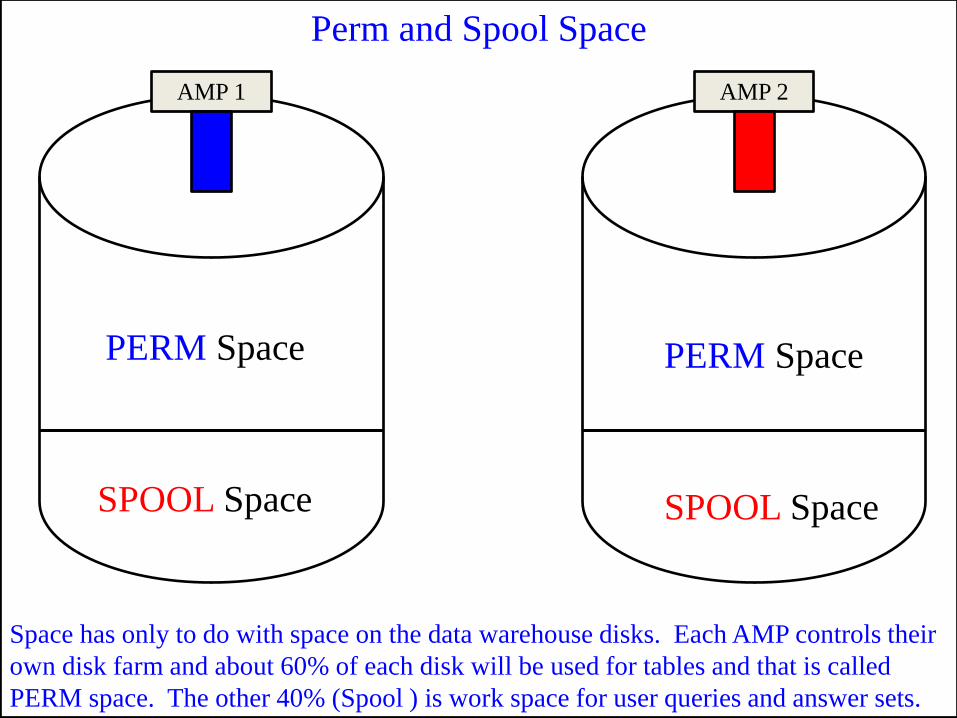
Perm and Spool Space
Space has only to do with space on the data warehouse disks. Each AMP controls their
own disk farm and about 60% of each disk will be used for tables and that is called
PERM space. The other 40% (Spool ) is work space for user queries and answer sets.
AMP 2 AMP 1
PERM Space
SPOOL Space
PERM Space
SPOOL Space
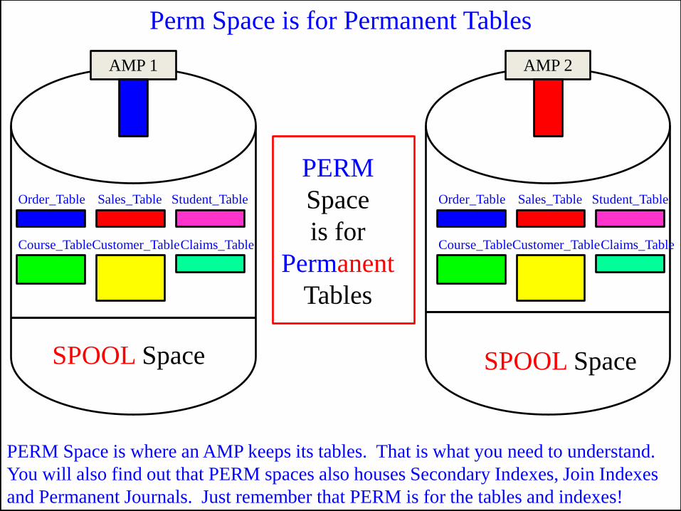
Perm Space is for Permanent Tables
PERM Space is where an AMP keeps its tables. That is what you need to understand.
You will also find out that PERM spaces also houses Secondary Indexes, Join Indexes
and Permanent Journals. Just remember that PERM is for the tables and indexes!
AMP 2 AMP 1
PERM
Space
is for
Permanent
Tables
SPOOL Space SPOOL Space
Order_Table Sales_Table Student_Table
Course_Table Customer_Table Claims_Table
Order_Table Sales_Table Student_Table
Course_Table Customer_Table Claims_Table
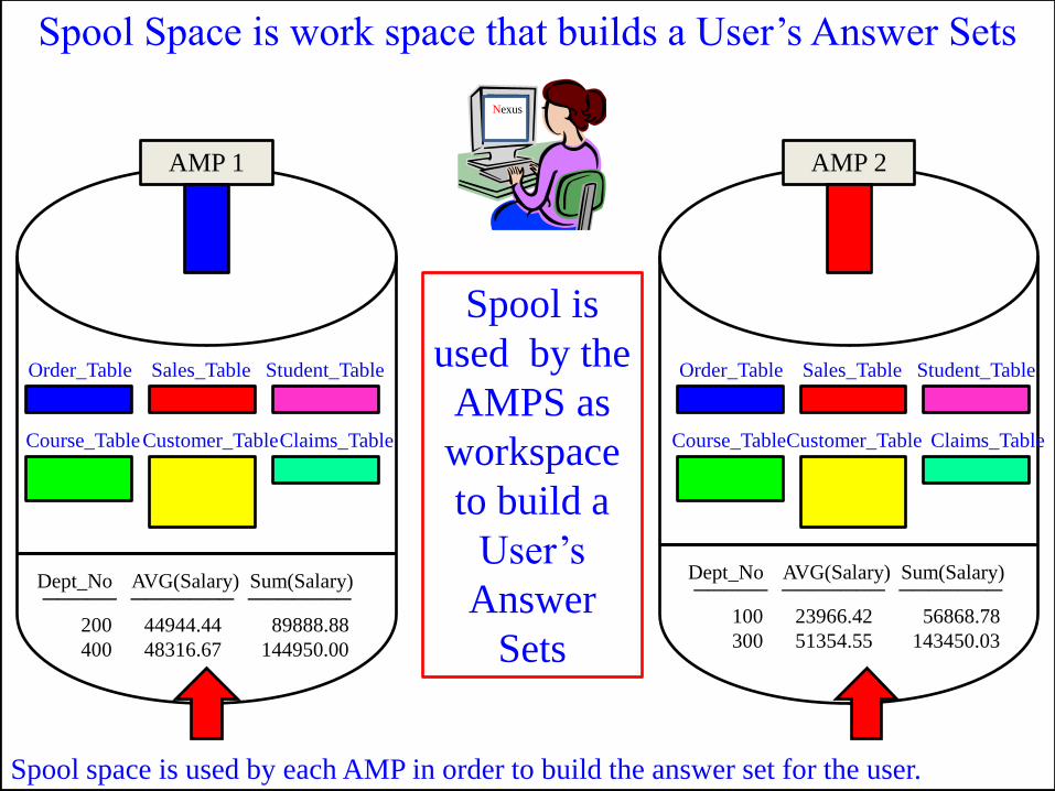
Spool Space is work space that builds a User‟s Answer Sets
Spool space is used by each AMP in order to build the answer set for the user.
AMP 2 AMP 1
Spool is
used by the
AMPS as
workspace
to build a
User‟s
Answer
Sets
Order_Table Sales_Table Student_Table
Course_Table Customer_Table Claims_Table
Order_Table Sales_Table Student_Table
Course_Table Customer_Table Claims_Table
Dept_No AVG(Salary) Sum(Salary)
44944.44
48316.67
200
400
89888.88
144950.00
_____ _______ _______ Dept_No AVG(Salary) Sum(Salary)
23966.42
51354.55
100
300
56868.78
143450.03
_____ _______ _______
Nexus
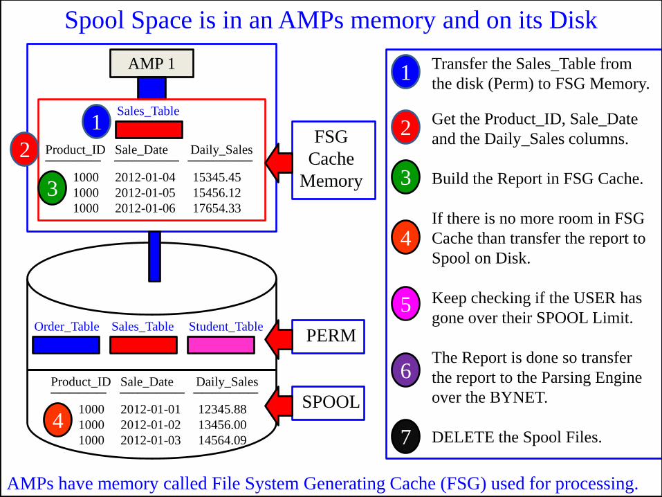
Spool Space is in an AMPs memory and on its Disk
AMPs have memory called File System Generating Cache (FSG) used for processing.
AMP 1
Order_Table Sales_Table Student_Table
Product_ID Sale_Date Daily_Sales
2012-01-01
2012-01-02
2012-01-03
1000
1000
1000
12345.88
13456.00
14564.09
______ _______ _______
Sales_Table
Product_ID Sale_Date Daily_Sales
2012-01-04
2012-01-05
2012-01-06
1000
1000
1000
15345.45
15456.12
17654.33
______ _______ _______ FSG
Cache
Memory
Transfer the Sales_Table from
the disk (Perm) to FSG Memory.
Get the Product_ID, Sale_Date
and the Daily_Sales columns.
Build the Report in FSG Cache.
If there is no more room in FSG
Cache than transfer the report to
Spool on Disk.
Keep checking if the USER has
gone over their SPOOL Limit.
The Report is done so transfer
the report to the Parsing Engine
over the BYNET.
DELETE the Spool Files.
PERM
SPOOL
1
2
3
4
5
6
7
1
2
3
4
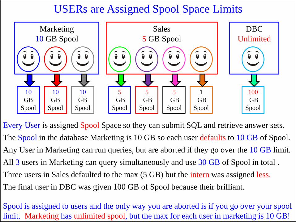
USERs are Assigned Spool Space Limits
Spool is assigned to users and the only way you are aborted is if you go over your spool
limit. Marketing has unlimited spool, but the max for each user in marketing is 10 GB!
Marketing
10 GB Spool
Sales
5 GB Spool
10
GB
Spool
10
GB
Spool
10
GB
Spool
5
GB
Spool
5
GB
Spool
5
GB
Spool
1
GB
Spool
100
GB
Spool
DBC
Unlimited
Every User is assigned Spool Space so they can submit SQL and retrieve answer sets.
The Spool in the database Marketing is 10 GB so each user defaults to 10 GB of Spool.
Any User in Marketing can run queries, but are aborted if they go over the 10 GB limit.
All 3 users in Marketing can query simultaneously and use 30 GB of Spool in total .
Three users in Sales defaulted to the max (5 GB) but the intern was assigned less.
The final user in DBC was given 100 GB of Spool because their brilliant.

What is the Purpose of Spool Limits?
Spool is assigned to users and the only way a user is aborted is if they go over their
spool limit. Marketing, Sales, and DBC have unlimited spool, but the max for each
individual user is 10 GB in Marketing, 5 GB in Sales, and our power user is at 100 GB.
Marketing
10 GB Spool
Sales
5 GB Spool
10
GB
Spool
10
GB
Spool
10
GB
Spool
5
GB
Spool
5
GB
Spool
5
GB
Spool
1
GB
Spool
100
GB
Spool
DBC
Unlimited
There are two reasons for Spool Limits:
If a user makes a mistake and runs a query that could take weeks to run it will
abort the second the user goes over their allotted spool limit.
It keeps users from hogging the system.
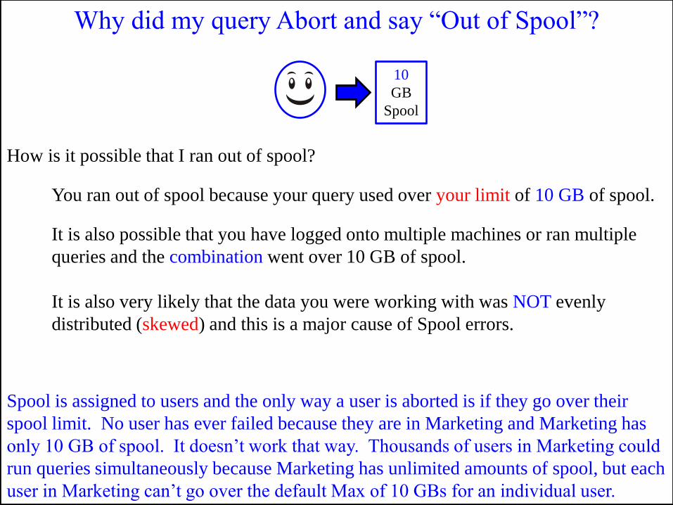
Why did my query Abort and say “Out of Spool”?
Spool is assigned to users and the only way a user is aborted is if they go over their
spool limit. No user has ever failed because they are in Marketing and Marketing has
only 10 GB of spool. It doesn‟t work that way. Thousands of users in Marketing could
run queries simultaneously because Marketing has unlimited amounts of spool, but each
user in Marketing can‟t go over the default Max of 10 GBs for an individual user.
10
GB
Spool
You ran out of spool because your query used over your limit of 10 GB of spool.
It is also possible that you have logged onto multiple machines or ran multiple
queries and the combination went over 10 GB of spool.
How is it possible that I ran out of spool?
It is also very likely that the data you were working with was NOT evenly
distributed (skewed) and this is a major cause of Spool errors.
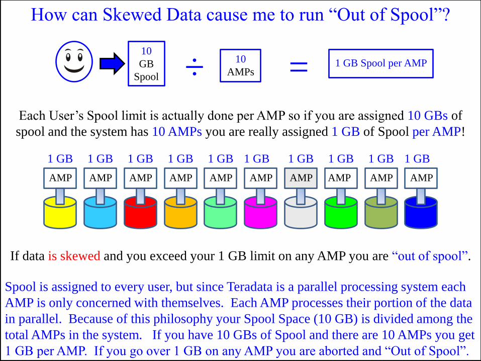
How can Skewed Data cause me to run “Out of Spool”?
Spool is assigned to every user, but since Teradata is a parallel processing system each
AMP is only concerned with themselves. Each AMP processes their portion of the data
in parallel. Because of this philosophy your Spool Space (10 GB) is divided among the
total AMPs in the system. If you have 10 GBs of Spool and there are 10 AMPs you get
1 GB per AMP. If you go over 1 GB on any AMP you are aborted and “Out of Spool”.
10
GB
Spool
AMP AMP AMP AMP AMP AMP AMP AMP AMP AMP
Each User‟s Spool limit is actually done per AMP so if you are assigned 10 GBs of
spool and the system has 10 AMPs you are really assigned 1 GB of Spool per AMP!
1 GB 1 GB 1 GB 1 GB 1 GB 1 GB 1 GB 1 GB 1 GB 1 GB
If data is skewed and you exceed your 1 GB limit on any AMP you are “out of spool”.
÷ = 10
AMPs 1 GB Spool per AMP
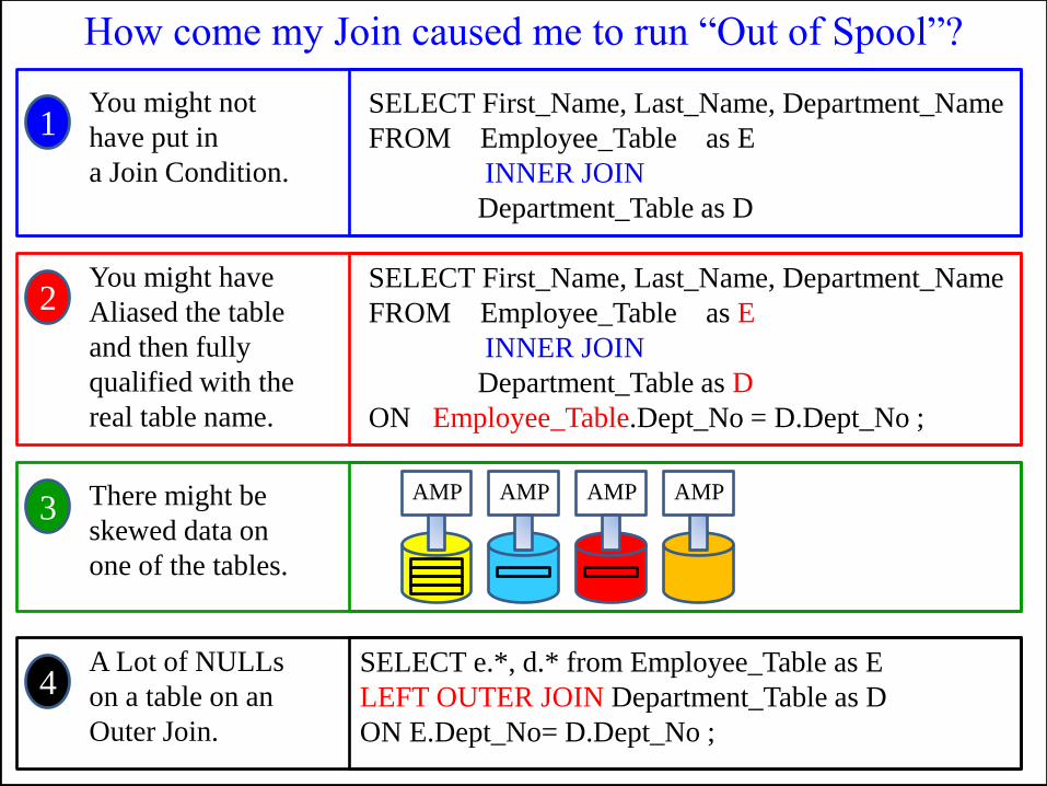
How come my Join caused me to run “Out of Spool”?
SELECT First_Name, Last_Name, Department_Name
FROM Employee_Table as E
INNER JOIN
Department_Table as D
1 You might not
have put in
a Join Condition.
SELECT First_Name, Last_Name, Department_Name
FROM Employee_Table as E
INNER JOIN
Department_Table as D
ON Employee_Table.Dept_No = D.Dept_No ;
2 You might have
Aliased the table
and then fully
qualified with the
real table name.
3 There might be
skewed data on
one of the tables.
AMP AMP AMP AMP
4 A Lot of NULLs
on a table on an
Outer Join.
SELECT e.*, d.* from Employee_Table as E
LEFT OUTER JOIN Department_Table as D
ON E.Dept_No= D.Dept_No ;
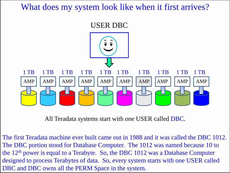
What does my system look like when it first arrives?
The first Teradata machine ever built came out in 1988 and it was called the DBC 1012.
The DBC portion stood for Database Computer. The 1012 was named because 10 to
the 12th power is equal to a Terabyte. So, the DBC 1012 was a Database Computer
designed to process Terabytes of data. So, every system starts with one USER called
DBC and DBC owns all the PERM Space in the system.
AMP AMP AMP AMP AMP AMP AMP AMP AMP AMP
1 TB 1 TB 1 TB 1 TB 1 TB 1 TB 1 TB 1 TB 1 TB 1 TB
All Teradata systems start with one USER called DBC.
USER DBC
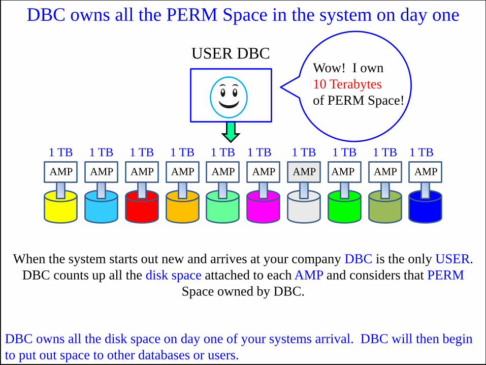
DBC owns all the PERM Space in the system on day one
DBC owns all the disk space on day one of your systems arrival. DBC will then begin
to put out space to other databases or users.
AMP AMP AMP AMP AMP AMP AMP AMP AMP AMP
1 TB 1 TB 1 TB 1 TB 1 TB 1 TB 1 TB 1 TB 1 TB 1 TB
When the system starts out new and arrives at your company DBC is the only USER.
DBC counts up all the disk space attached to each AMP and considers that PERM
Space owned by DBC.
USER DBC Wow! I own
10 Terabytes
of PERM Space!
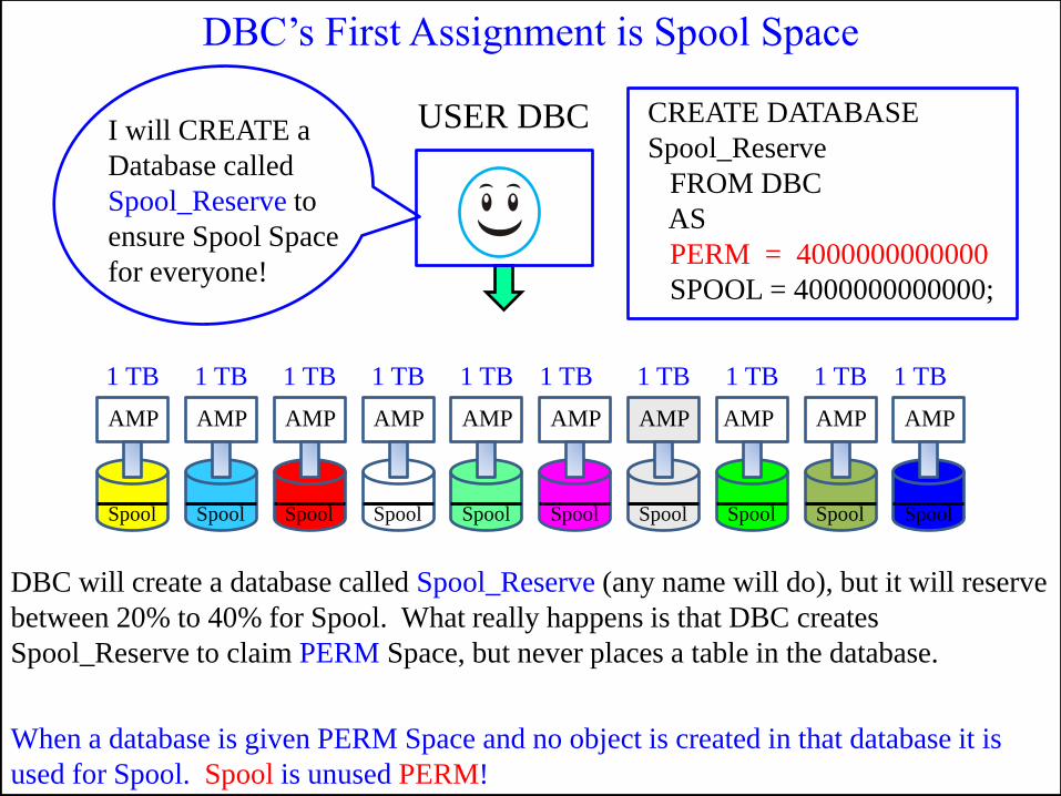
DBC‟s First Assignment is Spool Space
When a database is given PERM Space and no object is created in that database it is
used for Spool. Spool is unused PERM!
AMP AMP AMP AMP AMP AMP AMP AMP AMP AMP
1 TB 1 TB 1 TB 1 TB 1 TB 1 TB 1 TB 1 TB 1 TB 1 TB
DBC will create a database called Spool_Reserve (any name will do), but it will reserve
between 20% to 40% for Spool. What really happens is that DBC creates
Spool_Reserve to claim PERM Space, but never places a table in the database.
USER DBC I will CREATE a
Database called
Spool_Reserve to
ensure Spool Space
for everyone!
CREATE DATABASE
Spool_Reserve
FROM DBC
AS
PERM = 4000000000000
SPOOL = 4000000000000;
Spool Spool Spool Spool Spool Spool Spool Spool Spool Spool
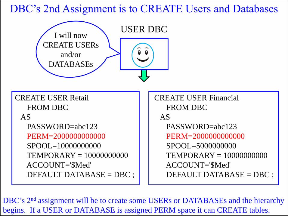
DBC‟s 2nd Assignment is to CREATE Users and Databases
DBC‟s 2nd assignment will be to create some USERs or DATABASEs and the hierarchy
begins. If a USER or DATABASE is assigned PERM space it can CREATE tables.
USER DBC I will now
CREATE USERs
and/or
DATABASEs
CREATE USER Retail
FROM DBC
AS
PASSWORD=abc123
PERM=2000000000000
SPOOL=10000000000
TEMPORARY = 10000000000
ACCOUNT='$Med'
DEFAULT DATABASE = DBC ;
CREATE USER Financial
FROM DBC
AS
PASSWORD=abc123
PERM=2000000000000
SPOOL=5000000000
TEMPORARY = 10000000000
ACCOUNT='$Med'
DEFAULT DATABASE = DBC ;
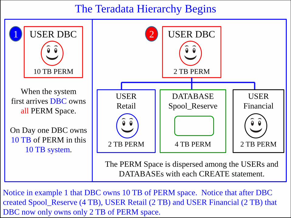
The Teradata Hierarchy Begins
Notice in example 1 that DBC owns 10 TB of PERM space. Notice that after DBC
created Spool_Reserve (4 TB), USER Retail (2 TB) and USER Financial (2 TB) that
DBC now only owns only 2 TB of PERM space.
USER DBC
2 TB PERM
2 TB PERM 2 TB PERM 4 TB PERM
USER
Retail
USER
Financial
DATABASE
Spool_Reserve
USER DBC
10 TB PERM
1
When the system
first arrives DBC owns
all PERM Space.
On Day one DBC owns
10 TB of PERM in this
10 TB system.
The PERM Space is dispersed among the USERs and
DATABASEs with each CREATE statement.
2
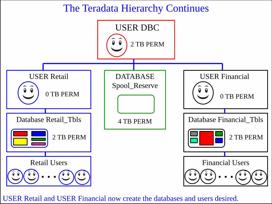
The Teradata Hierarchy Continues
USER Retail and USER Financial now create the databases and users desired.
USER DBC
2 TB PERM
0 TB PERM 0 TB PERM
4 TB PERM
USER Retail USER Financial DATABASE
Spool_Reserve
2 TB PERM
Database Retail_Tbls
2 TB PERM
Database Financial_Tbls
Retail Users
… Financial Users
…
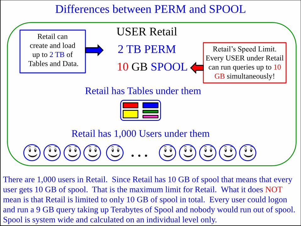
Differences between PERM and SPOOL
There are 1,000 users in Retail. Since Retail has 10 GB of spool that means that every
user gets 10 GB of spool. That is the maximum limit for Retail. What it does NOT
mean is that Retail is limited to only 10 GB of spool in total. Every user could logon
and run a 9 GB query taking up Terabytes of Spool and nobody would run out of spool.
Spool is system wide and calculated on an individual level only.
USER Retail
2 TB PERM
10 GB SPOOL
… Retail has 1,000 Users under them
Retail has Tables under them
Retail can
create and load
up to 2 TB of
Tables and Data.
Retail‟s Speed Limit.
Every USER under Retail
can run queries up to 10
GB simultaneously!
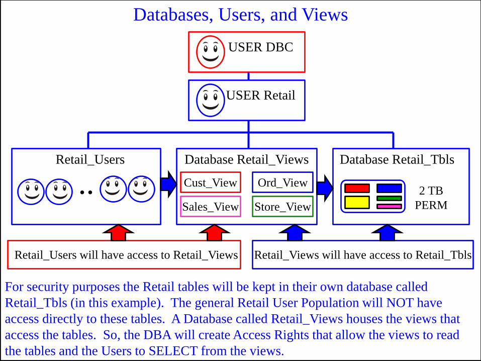
Databases, Users, and Views
For security purposes the Retail tables will be kept in their own database called
Retail_Tbls (in this example). The general Retail User Population will NOT have
access directly to these tables. A Database called Retail_Views houses the views that
access the tables. So, the DBA will create Access Rights that allow the views to read
the tables and the Users to SELECT from the views.
2 TB
PERM
Database Retail_Tbls Retail_Users
.. Database Retail_Views
Cust_View Ord_View
Sales_View Store_View
Retail_Users will have access to Retail_Views Retail_Views will have access to Retail_Tbls
USER DBC
USER Retail
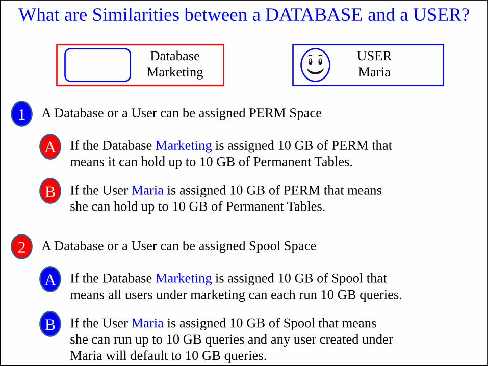
What are Similarities between a DATABASE and a USER?
Database
Marketing
USER
Maria
A Database or a User can be assigned PERM Space 1
If the Database Marketing is assigned 10 GB of PERM that
means it can hold up to 10 GB of Permanent Tables. A
If the User Maria is assigned 10 GB of PERM that means
she can hold up to 10 GB of Permanent Tables. B
A Database or a User can be assigned Spool Space 2
If the Database Marketing is assigned 10 GB of Spool that
means all users under marketing can each run 10 GB queries. A
If the User Maria is assigned 10 GB of Spool that means
she can run up to 10 GB queries and any user created under
Maria will default to 10 GB queries.
B
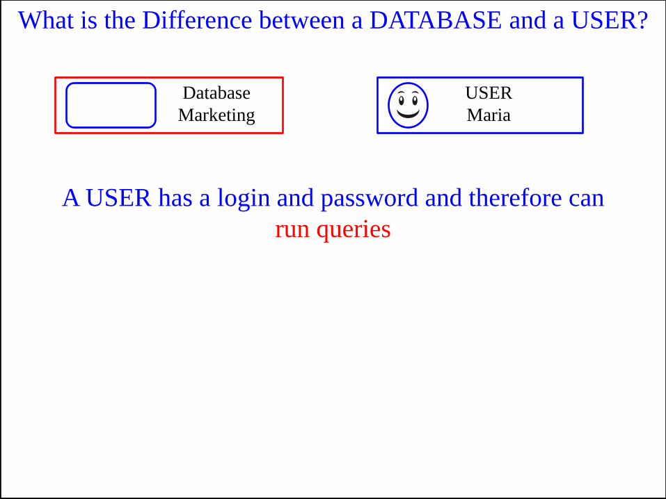
What is the Difference between a DATABASE and a USER?
A USER has a login and password and therefore can
run queries
Database
Marketing
USER
Maria
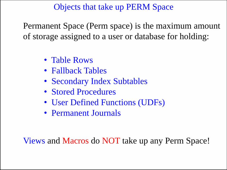
Objects that take up PERM Space
• Table Rows
• Fallback Tables
• Secondary Index Subtables
• Stored Procedures
• User Defined Functions (UDFs)
• Permanent Journals
Permanent Space (Perm space) is the maximum amount
of storage assigned to a user or database for holding:
Views and Macros do NOT take up any Perm Space!

A Series of Quizzes on Adding and Subtracting Space
After creating users how much Perm / Spool is in Marketing and how much is in Sales?
Marketing
10 GB Perm
10 GB Spool
Sales
5 GB Perm
5 GB Spool
Marketing has 10 GB of Perm and Spool. Sales has 5 GB Perm and Spool. 1
2 Marketing then Creates Stan and gives him 1 GB Perm and 10 GB Spool.
3 Sales then Creates Mary and gives her 1 GB Perm and 5 GB Spool.
Marketing Sales
Stan
1 GB Perm
10 GB Spool
Mary
1 GB Perm
5 GB Spool
_____________ ________________ _______________ _____________

Answer 1 to Quiz on Space
After creating users how much Perm / Spool is in Marketing and how much is in Sales?
Marketing
10 GB Perm
10 GB Spool
Sales
5 GB Perm
5 GB Spool
Marketing has 10 GB of Perm and Spool. Sales has 5 GB Perm and Spool. 1
2 Marketing then Creates Stan and gives him 1 GB Perm and 10 GB Spool.
3 Sales then Creates Mary and gives her 1 GB Perm and 5 GB Spool.
Marketing Sales
Stan
1 GB Perm
10 GB Spool
Mary
1 GB Perm
5 GB Spool
_____________ ________________ _______________ _____________ 9 GB Perm 10 GB Spool 4 GB Perm 5 GB Spool

Space Transfer Quiz
Stan has just been transferred to Sales.
If a USER is dropped their PERM Space goes up to their immediate parent. 1
2 If a USER is transferred (GIVE Statement) they take their space with them.
Marketing
9 GB Perm
10 GB Spool
Stan
1 GB Perm
10 GB Spool
Mary
1 GB Perm
5 GB Spool
_____________ ________________
Sales
4 GB Perm
5 GB Spool
After the transfer how much Perm / Spool is in:
Marketing
Sales
Stan
_____________ ________________
_____________ ________________
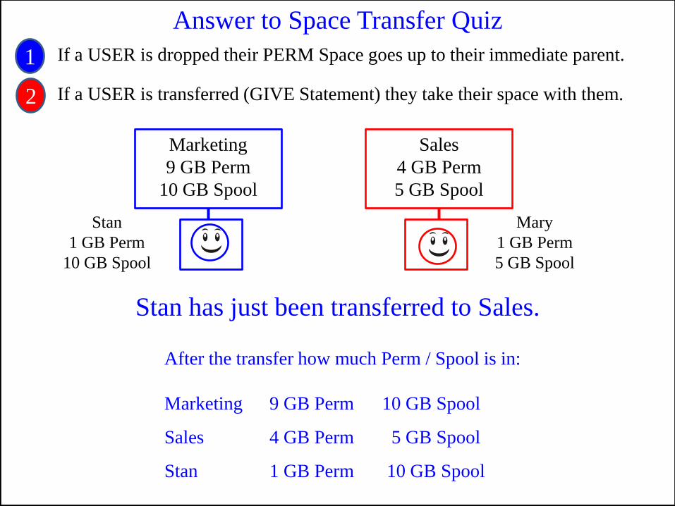
Answer to Space Transfer Quiz
Stan has just been transferred to Sales.
If a USER is dropped their PERM Space goes up to their immediate parent. 1
2 If a USER is transferred (GIVE Statement) they take their space with them.
Marketing
9 GB Perm
10 GB Spool
Stan
1 GB Perm
10 GB Spool
Mary
1 GB Perm
5 GB Spool
9 GB Perm 10 GB Spool
Sales
4 GB Perm
5 GB Spool
After the transfer how much Perm / Spool is in:
Marketing
Sales
Stan
4 GB Perm 5 GB Spool
1 GB Perm 10 GB Spool

Drop Space Quiz
What happens NOW if Stan is Dropped?
If a USER is dropped their PERM Space goes up to their immediate parent. 1
2 If a USER is transferred (GIVE Statement) they take their space with them.
Marketing
9 GB Perm
10 GB Spool
Mary
1 GB Perm
5 GB Spool
Sales
4 GB Perm
5 GB Spool
Stan
1 GB Perm
10 GB Spool
___________ ___________
After the drop how much Perm / Spool is in:
Marketing
Sales
Stan
___________ ___________
___________ ___________

Answers to Drop Space Quiz
What happens NOW if Stan is Dropped?
If a USER is dropped their PERM Space goes up to their immediate parent. 1
2 If a USER is transferred (GIVE Statement) they take their space with them.
Marketing
9 GB Perm
10 GB Spool
Mary
1 GB Perm
5 GB Spool
Sales
4 GB Perm
5 GB Spool
Stan
1 GB Perm
10 GB Spool
9 GB Perm 10 GB Spool
After the drop how much Perm / Spool is in:
Marketing
Sales
Stan
5 GB Perm 5 GB Spool
dropped (0) dropped (0)

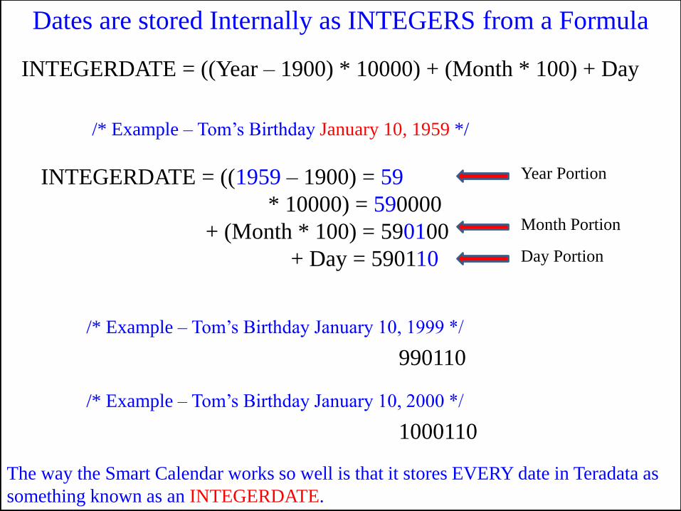
The way the Smart Calendar works so well is that it stores EVERY date in Teradata as
something known as an INTEGERDATE.
Dates are stored Internally as INTEGERS from a Formula
INTEGERDATE = ((Year – 1900) * 10000) + (Month * 100) + Day
990110
/* Example – Tom‟s Birthday January 10, 1959 */
INTEGERDATE = ((1959 – 1900) = 59
* 10000) = 590000
+ (Month * 100) = 590100
+ Day = 590110
/* Example – Tom‟s Birthday January 10, 1999 */
1000110
/* Example – Tom‟s Birthday January 10, 2000 */
Year Portion
Month Portion
Day Portion
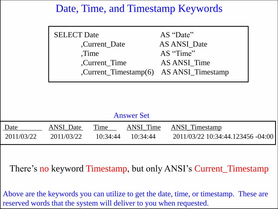
Above are the keywords you can utilize to get the date, time, or timestamp. These are
reserved words that the system will deliver to you when requested.
SELECT Date AS “Date”
,Current_Date AS ANSI_Date
,Time AS “Time”
,Current_Time AS ANSI_Time
,Current_Timestamp(6) AS ANSI_Timestamp
Date ANSI_Date Time ANSI_Time ANSI_Timestamp
2011/03/22 2011/03/22 10:34:44 10:34:44 2011/03/22 10:34:44.123456 -04:00
Date, Time, and Timestamp Keywords
Answer Set
There‟s no keyword Timestamp, but only ANSI‟s Current_Timestamp
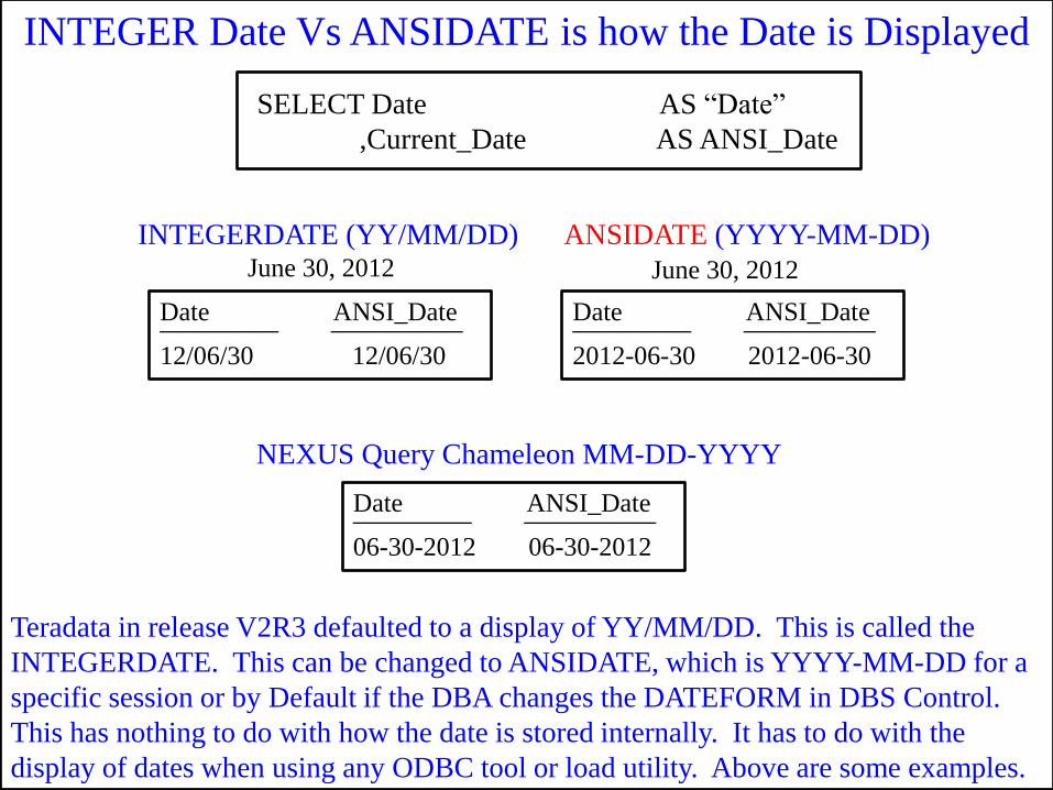
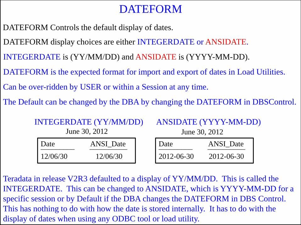
Teradata in release V2R3 defaulted to a display of YY/MM/DD. This is called the
INTEGERDATE. This can be changed to ANSIDATE, which is YYYY-MM-DD for a
specific session or by Default if the DBA changes the DATEFORM in DBS Control.
This has nothing to do with how the date is stored internally. It has to do with the
display of dates when using any ODBC tool or load utility. Above are some examples.
SELECT Date AS “Date”
,Current_Date AS ANSI_Date
INTEGER Date Vs ANSIDATE is how the Date is Displayed
Date ANSI_Date
2012-06-30 2012-06-30
_________ __________ Date ANSI_Date
12/06/30 12/06/30
_________ __________
June 30, 2012 June 30, 2012
INTEGERDATE (YY/MM/DD) ANSIDATE (YYYY-MM-DD)
Date ANSI_Date
06-30-2012 06-30-2012
_________ __________
NEXUS Query Chameleon MM-DD-YYYY
Teradata in release V2R3 defaulted to a display of YY/MM/DD. This is called the
INTEGERDATE. This can be changed to ANSIDATE, which is YYYY-MM-DD for a
specific session or by Default if the DBA changes the DATEFORM in DBS Control.
This has nothing to do with how the date is stored internally. It has to do with the
display of dates when using any ODBC tool or load utility.
DATEFORM
Date ANSI_Date
2012-06-30 2012-06-30
_________ __________ Date ANSI_Date
12/06/30 12/06/30
_________ __________
June 30, 2012 June 30, 2012
INTEGERDATE (YY/MM/DD) ANSIDATE (YYYY-MM-DD)
DATEFORM Controls the default display of dates.
DATEFORM display choices are either INTEGERDATE or ANSIDATE.
INTEGERDATE is (YY/MM/DD) and ANSIDATE is (YYYY-MM-DD).
DATEFORM is the expected format for import and export of dates in Load Utilities.
Can be over-ridden by USER or within a Session at any time.
The Default can be changed by the DBA by changing the DATEFORM in DBSControl.
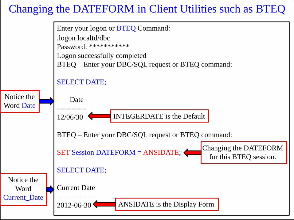
Changing the DATEFORM in Client Utilities such as BTEQ
Enter your logon or BTEQ Command:
.logon localtd/dbc
Password: ***********
Logon successfully completed
BTEQ – Enter your DBC/SQL request or BTEQ command:
SELECT DATE;
Date
------------
12/06/30
BTEQ – Enter your DBC/SQL request or BTEQ command:
SET Session DATEFORM = ANSIDATE;
SELECT DATE;
Current Date
----------------
2012-06-30
INTEGERDATE is the Default
Changing the DATEFORM
for this BTEQ session.
ANSIDATE is the Display Form
Notice the
Word Date
Notice the
Word
Current_Date
SELECT Date AS “Date”
,Current_Date AS ANSI_Date
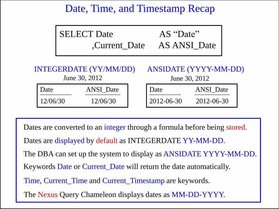
Date, Time, and Timestamp Recap
Dates are converted to an integer through a formula before being stored.
Dates are displayed by default as INTEGERDATE YY-MM-DD.
The DBA can set up the system to display as ANSIDATE YYYY-MM-DD.
Keywords Date or Current_Date will return the date automatically.
Time, Current_Time and Current_Timestamp are keywords.
The Nexus Query Chameleon displays dates as MM-DD-YYYY.
Date ANSI_Date
2012-06-30 2012-06-30
_________ __________ Date ANSI_Date
12/06/30 12/06/30
_________ __________
June 30, 2012 June 30, 2012
INTEGERDATE (YY/MM/DD) ANSIDATE (YYYY-MM-DD)
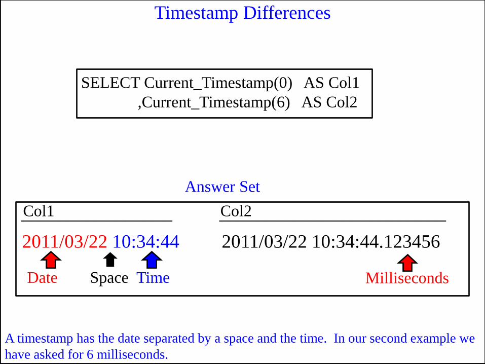
A timestamp has the date separated by a space and the time. In our second example we
have asked for 6 milliseconds.
SELECT Current_Timestamp(0) AS Col1
,Current_Timestamp(6) AS Col2
Col1 Col2
2011/03/22 10:34:44 2011/03/22 10:34:44.123456
Timestamp Differences
Answer Set
Date Space Time Milliseconds
________________ ________________________
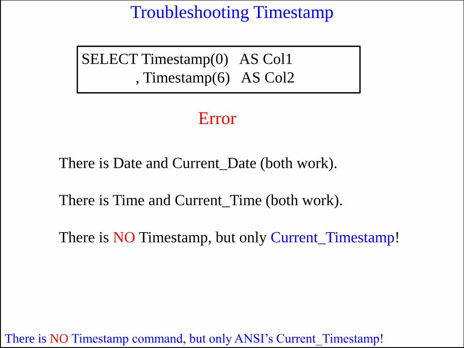
There is NO Timestamp command, but only ANSI‟s Current_Timestamp!
SELECT Timestamp(0) AS Col1
, Timestamp(6) AS Col2
Troubleshooting Timestamp
There is Date and Current_Date (both work).
There is Time and Current_Time (both work).
There is NO Timestamp, but only Current_Timestamp!
Error
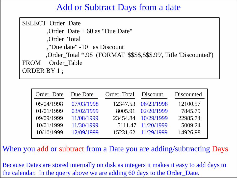
SELECT Order_Date
,Order_Date + 60 as "Due Date"
,Order_Total
,"Due date" -10 as Discount
,Order_Total *.98 (FORMAT '$$$$,$$$.99', Title 'Discounted')
FROM Order_Table
ORDER BY 1 ;
Because Dates are stored internally on disk as integers it makes it easy to add days to
the calendar. In the query above we are adding 60 days to the Order_Date.
When you add or subtract from a Date you are adding/subtracting Days
Add or Subtract Days from a date
Order_Date Due Date Order_Total Discount Discounted
05/04/1998
01/01/1999
09/09/1999
10/01/1999
10/10/1999
07/03/1998
03/02/1999
11/08/1999
11/30/1999
12/09/1999
12347.53
8005.91
23454.84
5111.47
15231.62
__________ _________ __________ _________ __________
06/23/1998
02/20/1999
10/29/1999
11/20/1999
11/29/1999
12100.57
7845.79
22985.74
5009.24
14926.98
A DATE – DATE is an interval of days between dates. A DATE + or – Integer = Date.
Both queries above perform the same function, but the top query uses the internal date
functions and the query on the bottom does dates the traditional way.
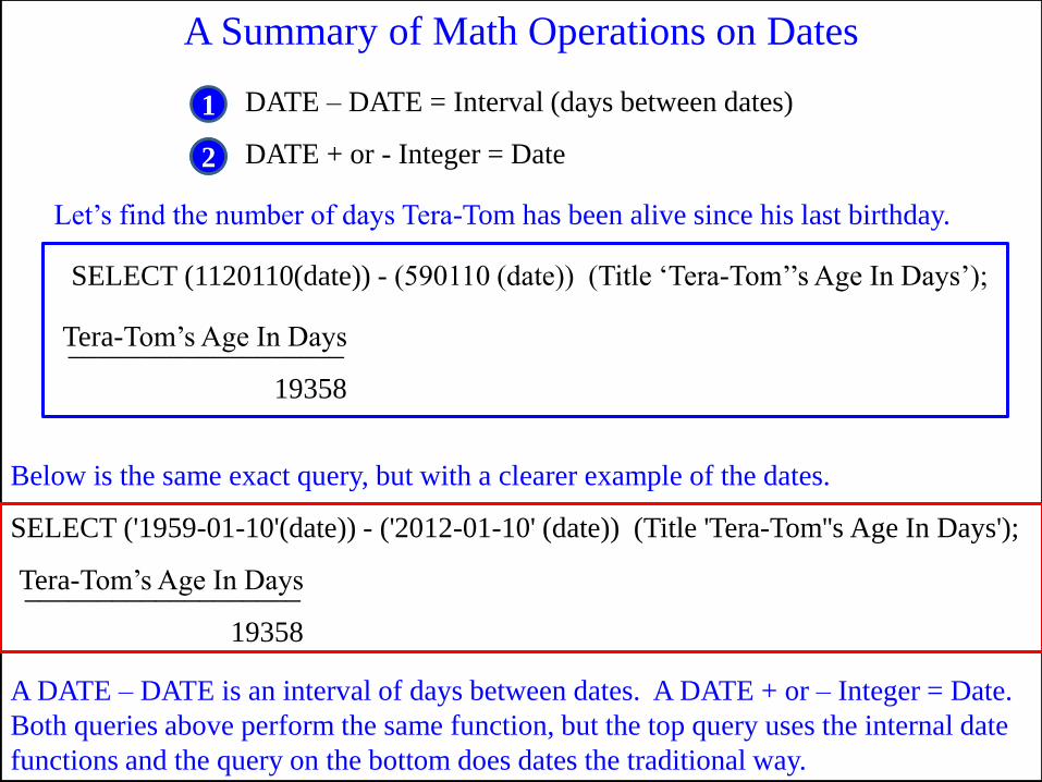
A Summary of Math Operations on Dates
DATE – DATE = Interval (days between dates)
DATE + or - Integer = Date
SELECT (1120110(date)) - (590110 (date)) (Title „Tera-Tom‟‟s Age In Days‟);
19358
Tera-Tom‟s Age In Days ___________________
SELECT ('1959-01-10'(date)) - ('2012-01-10' (date)) (Title 'Tera-Tom''s Age In Days');
19358
Tera-Tom‟s Age In Days ___________________
Let‟s find the number of days Tera-Tom has been alive since his last birthday.
Below is the same exact query, but with a clearer example of the dates.
1
2
A DATE – DATE is an interval of days between dates. A DATE + or – Integer = Date.
Both queries above perform the same function, but the top query uses the internal date
functions and the query on the bottom does dates the traditional way.
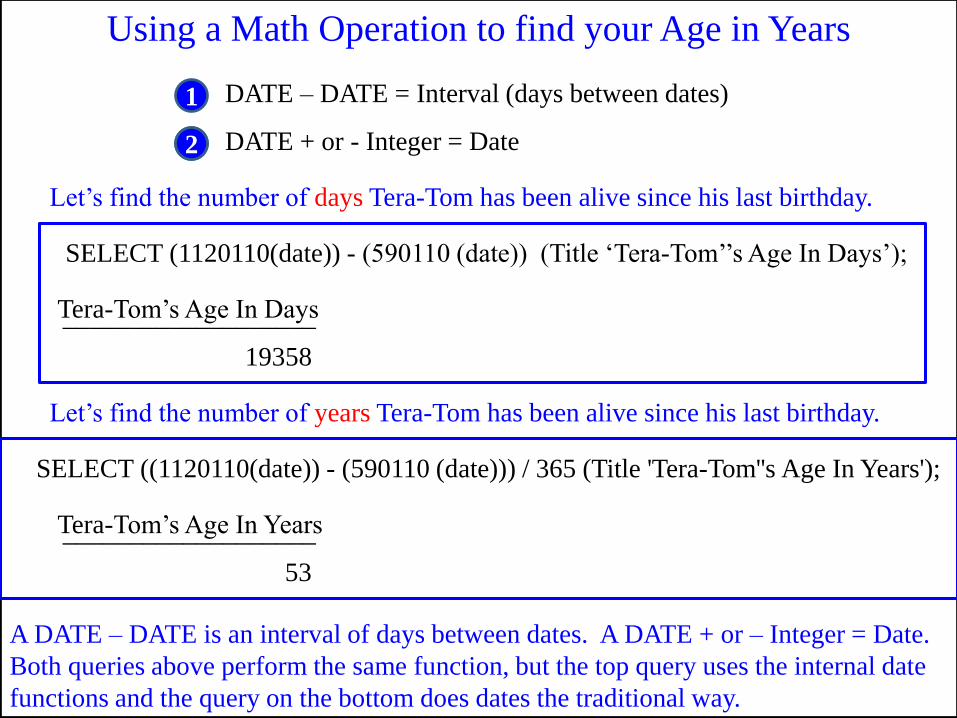
Using a Math Operation to find your Age in Years
DATE – DATE = Interval (days between dates)
DATE + or - Integer = Date
SELECT (1120110(date)) - (590110 (date)) (Title „Tera-Tom‟‟s Age In Days‟);
19358
Tera-Tom‟s Age In Days ___________________
Let‟s find the number of days Tera-Tom has been alive since his last birthday.
1
2
SELECT ((1120110(date)) - (590110 (date))) / 365 (Title 'Tera-Tom''s Age In Years');
53
Tera-Tom‟s Age In Years ___________________
Let‟s find the number of years Tera-Tom has been alive since his last birthday.
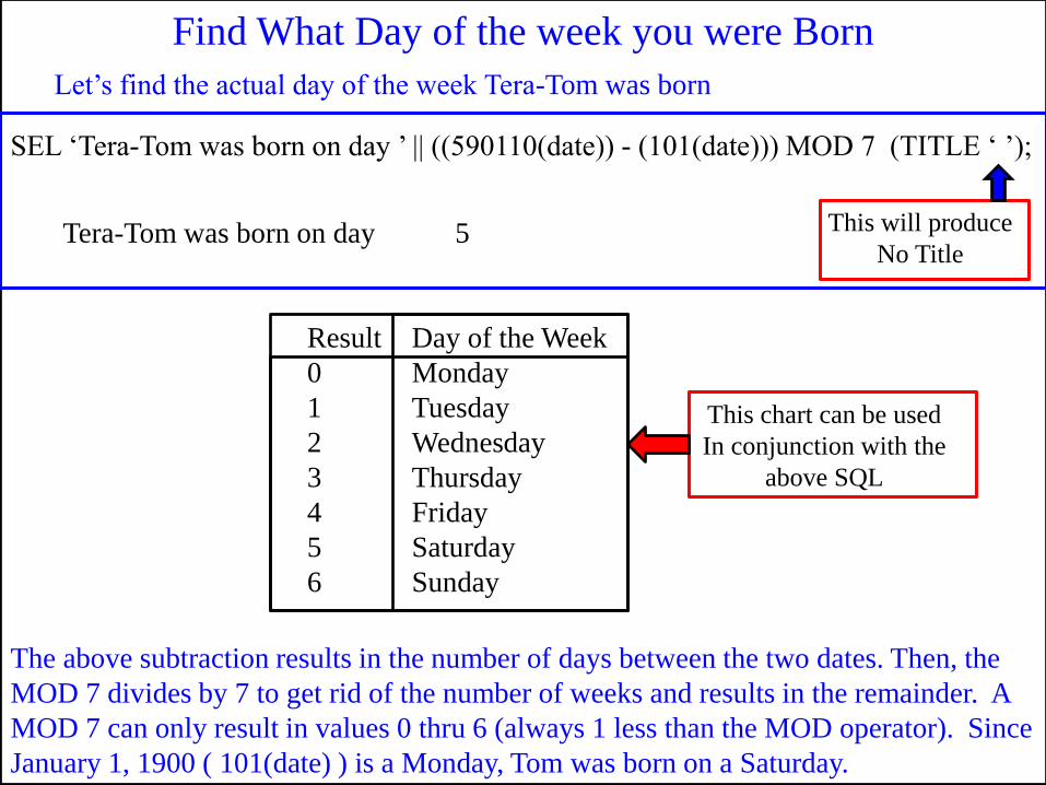
Find What Day of the week you were Born
SEL „Tera-Tom was born on day ‟ || ((590110(date)) - (101(date))) MOD 7 (TITLE „ ‟);
Tera-Tom was born on day 5
Let‟s find the actual day of the week Tera-Tom was born
This will produce
No Title
The above subtraction results in the number of days between the two dates. Then, the
MOD 7 divides by 7 to get rid of the number of weeks and results in the remainder. A
MOD 7 can only result in values 0 thru 6 (always 1 less than the MOD operator). Since
January 1, 1900 ( 101(date) ) is a Monday, Tom was born on a Saturday.
Result Day of the Week
0 Monday
1 Tuesday
2 Wednesday
3 Thursday
4 Friday
5 Saturday
6 Sunday
This chart can be used
In conjunction with the
above SQL
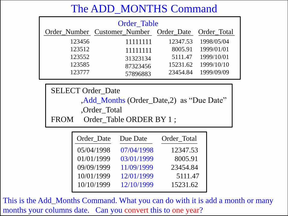
This is the Add_Months Command. What you can do with it is add a month or many
months your columns date. Can you convert this to one year?
SELECT Order_Date
,Add_Months (Order_Date,2) as “Due Date”
,Order_Total
FROM Order_Table ORDER BY 1 ;
Order_Number Customer_Number Order_Date Order_Total Order_Table
123456
123512
123552
123585
123777
11111111
11111111 31323134
87323456
57896883
12347.53
8005.91
5111.47
15231.62
23454.84
1998/05/04
1999/01/01
1999/10/01
1999/10/10
1999/09/09
The ADD_MONTHS Command
_____________ ________________ __________ __________
Order_Date Due Date Order_Total
05/04/1998
01/01/1999
09/09/1999
10/01/1999
10/10/1999
07/04/1998
03/01/1999
11/09/1999
12/01/1999
12/10/1999
12347.53
8005.91
23454.84
5111.47
15231.62
__________ _________ __________
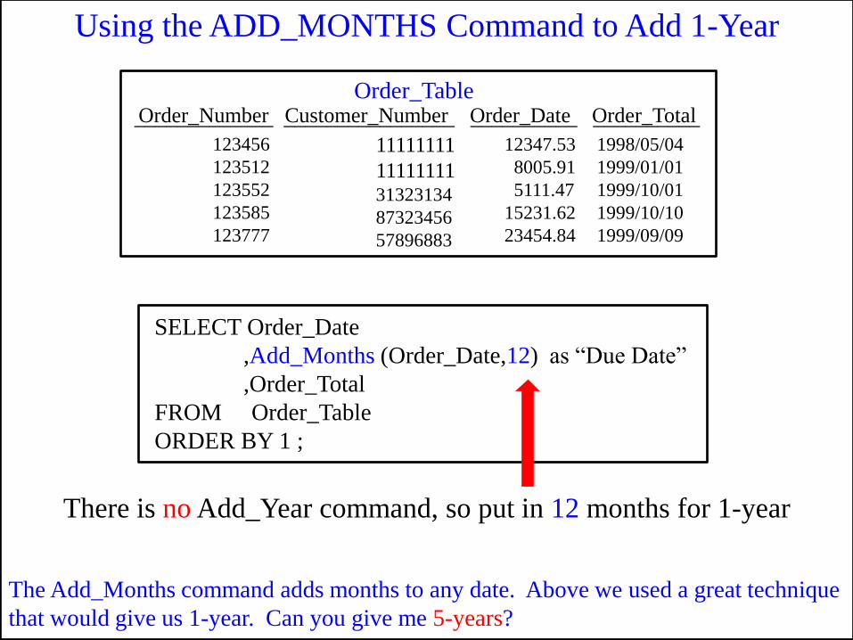
The Add_Months command adds months to any date. Above we used a great technique
that would give us 1-year. Can you give me 5-years?
SELECT Order_Date
,Add_Months (Order_Date,12) as “Due Date”
,Order_Total
FROM Order_Table
ORDER BY 1 ;
There is no Add_Year command, so put in 12 months for 1-year
Using the ADD_MONTHS Command to Add 1-Year
Order_Number Customer_Number Order_Date Order_Total Order_Table
123456
123512
123552
123585
123777
11111111
11111111 31323134
87323456
57896883
12347.53
8005.91
5111.47
15231.62
23454.84
1998/05/04
1999/01/01
1999/10/01
1999/10/10
1999/09/09
_____________ ________________ __________ __________
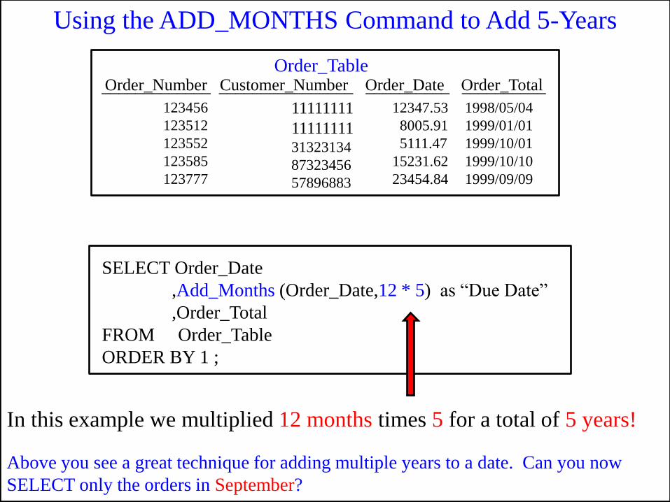
Above you see a great technique for adding multiple years to a date. Can you now
SELECT only the orders in September?
SELECT Order_Date
,Add_Months (Order_Date,12 * 5) as “Due Date”
,Order_Total
FROM Order_Table
ORDER BY 1 ;
In this example we multiplied 12 months times 5 for a total of 5 years!
Using the ADD_MONTHS Command to Add 5-Years
Order_Number Customer_Number Order_Date Order_Total Order_Table
123456
123512
123552
123585
123777
11111111
11111111 31323134
87323456
57896883
12347.53
8005.91
5111.47
15231.62
23454.84
1998/05/04
1999/01/01
1999/10/01
1999/10/10
1999/09/09
_____________ ________________ __________ __________
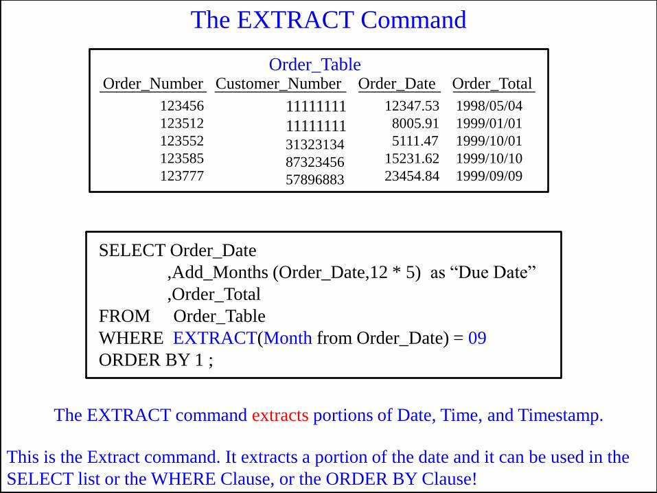
This is the Extract command. It extracts a portion of the date and it can be used in the
SELECT list or the WHERE Clause, or the ORDER BY Clause!
SELECT Order_Date
,Add_Months (Order_Date,12 * 5) as “Due Date”
,Order_Total
FROM Order_Table
WHERE EXTRACT(Month from Order_Date) = 09
ORDER BY 1 ;
The EXTRACT command extracts portions of Date, Time, and Timestamp.
The EXTRACT Command
Order_Number Customer_Number Order_Date Order_Total Order_Table
123456
123512
123552
123585
123777
11111111
11111111 31323134
87323456
57896883
12347.53
8005.91
5111.47
15231.62
23454.84
1998/05/04
1999/01/01
1999/10/01
1999/10/10
1999/09/09
_____________ ________________ __________ __________
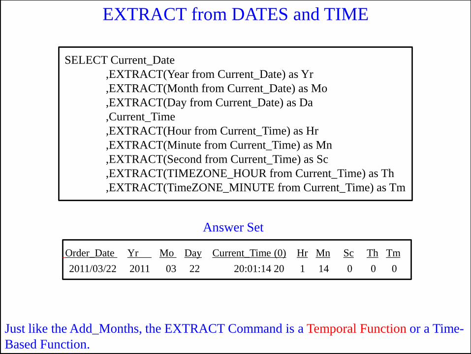
Just like the Add_Months, the EXTRACT Command is a Temporal Function or a Time-
Based Function.
EXTRACT from DATES and TIME
Order_Date Yr Mo Day Current_Time (0) Hr Mn Sc Th Tm
2011/03/22 2011 03 22 20:01:14 20 1 14 0 0 0
Answer Set
SELECT Current_Date
,EXTRACT(Year from Current_Date) as Yr
,EXTRACT(Month from Current_Date) as Mo
,EXTRACT(Day from Current_Date) as Da
,Current_Time
,EXTRACT(Hour from Current_Time) as Hr
,EXTRACT(Minute from Current_Time) as Mn
,EXTRACT(Second from Current_Time) as Sc
,EXTRACT(TIMEZONE_HOUR from Current_Time) as Th
,EXTRACT(TimeZONE_MINUTE from Current_Time) as Tm
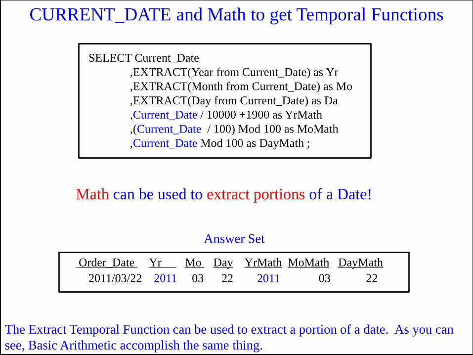
The Extract Temporal Function can be used to extract a portion of a date. As you can
see, Basic Arithmetic accomplish the same thing.
CURRENT_DATE and Math to get Temporal Functions
Order_Date Yr Mo Day YrMath MoMath DayMath
2011/03/22 2011 03 22 2011 03 22
Answer Set
SELECT Current_Date
,EXTRACT(Year from Current_Date) as Yr
,EXTRACT(Month from Current_Date) as Mo
,EXTRACT(Day from Current_Date) as Da
,Current_Date / 10000 +1900 as YrMath
,(Current_Date / 100) Mod 100 as MoMath
,Current_Date Mod 100 as DayMath ;
Math can be used to extract portions of a Date!
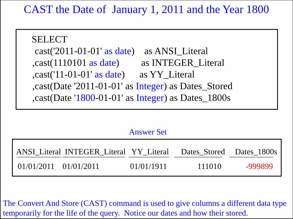
The Convert And Store (CAST) command is used to give columns a different data type
temporarily for the life of the query. Notice our dates and how their stored.
CAST the Date of January 1, 2011 and the Year 1800
Answer Set
SELECT
cast('2011-01-01' as date) as ANSI_Literal
,cast(1110101 as date) as INTEGER_Literal
,cast('11-01-01' as date) as YY_Literal
,cast(Date '2011-01-01' as Integer) as Dates_Stored
,cast(Date '1800-01-01' as Integer) as Dates_1800s
ANSI_Literal INTEGER_Literal YY_Literal Dates_Stored Dates_1800s
01/01/2011 01/01/2011 01/01/1911 111010 -999899
____________ _________________ ___________ _____________ ____________
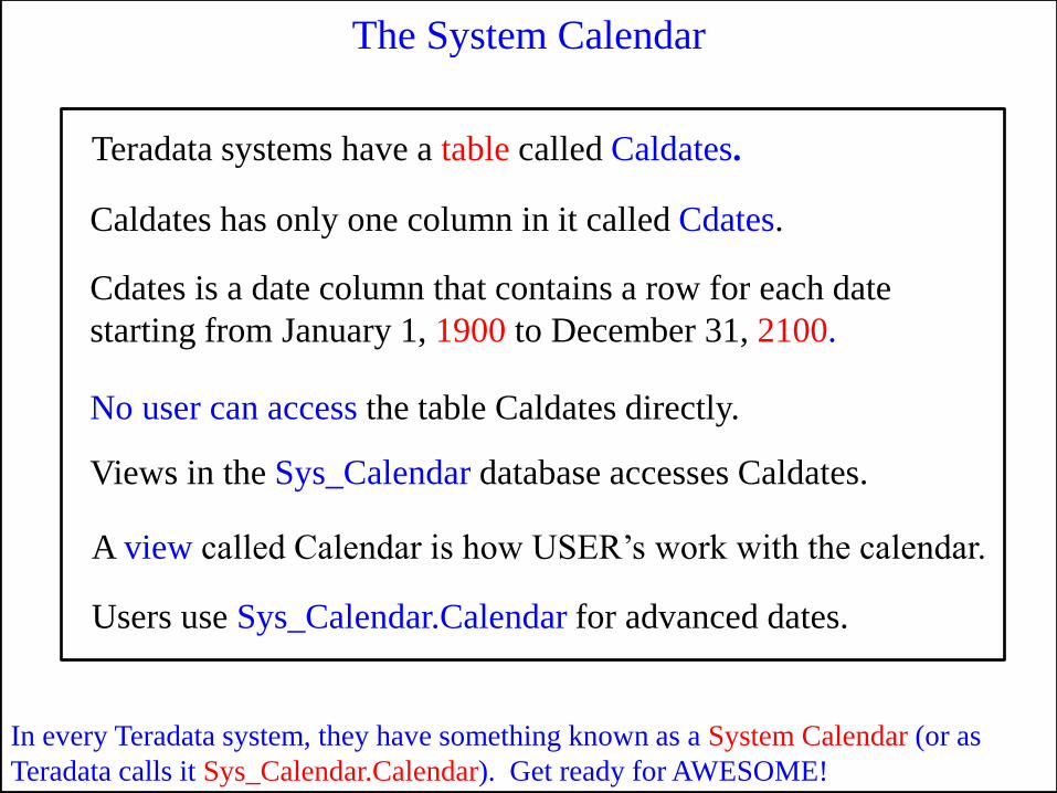
In every Teradata system, they have something known as a System Calendar (or as
Teradata calls it Sys_Calendar.Calendar). Get ready for AWESOME!
The System Calendar
Teradata systems have a table called Caldates.
Caldates has only one column in it called Cdates.
Cdates is a date column that contains a row for each date
starting from January 1, 1900 to December 31, 2100.
No user can access the table Caldates directly.
Views in the Sys_Calendar database accesses Caldates.
A view called Calendar is how USER‟s work with the calendar.
Users use Sys_Calendar.Calendar for advanced dates.
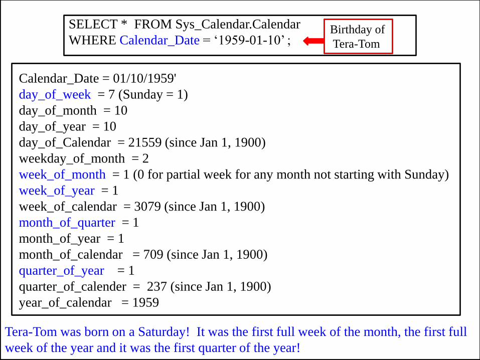
Tera-Tom was born on a Saturday! It was the first full week of the month, the first full
week of the year and it was the first quarter of the year!
SELECT * FROM Sys_Calendar.Calendar
WHERE Calendar_Date = „1959-01-10‟ ; Birthday of
Tera-Tom
Calendar_Date = 01/10/1959'
day_of_week = 7 (Sunday = 1)
day_of_month = 10
day_of_year = 10
day_of_Calendar = 21559 (since Jan 1, 1900)
weekday_of_month = 2
week_of_month = 1 (0 for partial week for any month not starting with Sunday)
week_of_year = 1
week_of_calendar = 3079 (since Jan 1, 1900)
month_of_quarter = 1
month_of_year = 1
month_of_calendar = 709 (since Jan 1, 1900)
quarter_of_year = 1
quarter_of_calender = 237 (since Jan 1, 1900)
year_of_calendar = 1959
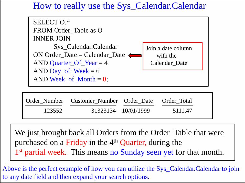
Above is the perfect example of how you can utilize the Sys_Calendar.Calendar to join
to any date field and then expand your search options.
SELECT O.*
FROM Order_Table as O
INNER JOIN
Sys_Calendar.Calendar
ON Order_Date = Calendar_Date
AND Quarter_Of_Year = 4
AND Day_of_Week = 6
AND Week_of_Month = 0;
How to really use the Sys_Calendar.Calendar
Join a date column
with the
Calendar_Date
Order_Number Customer_Number Order_Date Order_Total ____________ _______________ __________ __________
123552 31323134 10/01/1999 5111.47
We just brought back all Orders from the Order_Table that were
purchased on a Friday in the 4th Quarter, during the
1st partial week. This means no Sunday seen yet for that month.
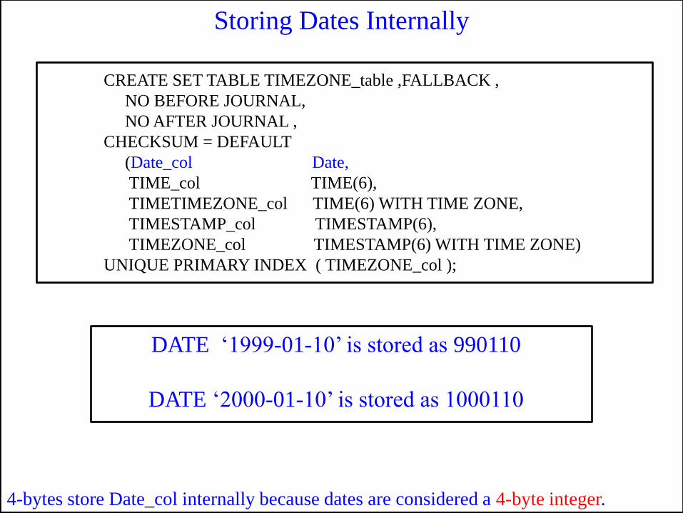
4-bytes store Date_col internally because dates are considered a 4-byte integer.
CREATE SET TABLE TIMEZONE_table ,FALLBACK ,
NO BEFORE JOURNAL,
NO AFTER JOURNAL ,
CHECKSUM = DEFAULT
(Date_col Date,
TIME_col TIME(6),
TIMETIMEZONE_col TIME(6) WITH TIME ZONE,
TIMESTAMP_col TIMESTAMP(6),
TIMEZONE_col TIMESTAMP(6) WITH TIME ZONE)
UNIQUE PRIMARY INDEX ( TIMEZONE_col );
DATE „1999-01-10‟ is stored as 990110
DATE „2000-01-10‟ is stored as 1000110
Storing Dates Internally
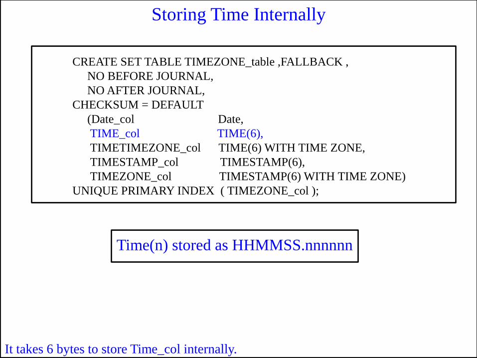
It takes 6 bytes to store Time_col internally.
Storing Time Internally
CREATE SET TABLE TIMEZONE_table ,FALLBACK ,
NO BEFORE JOURNAL,
NO AFTER JOURNAL,
CHECKSUM = DEFAULT
(Date_col Date,
TIME_col TIME(6),
TIMETIMEZONE_col TIME(6) WITH TIME ZONE,
TIMESTAMP_col TIMESTAMP(6),
TIMEZONE_col TIMESTAMP(6) WITH TIME ZONE)
UNIQUE PRIMARY INDEX ( TIMEZONE_col );
Time(n) stored as HHMMSS.nnnnnn
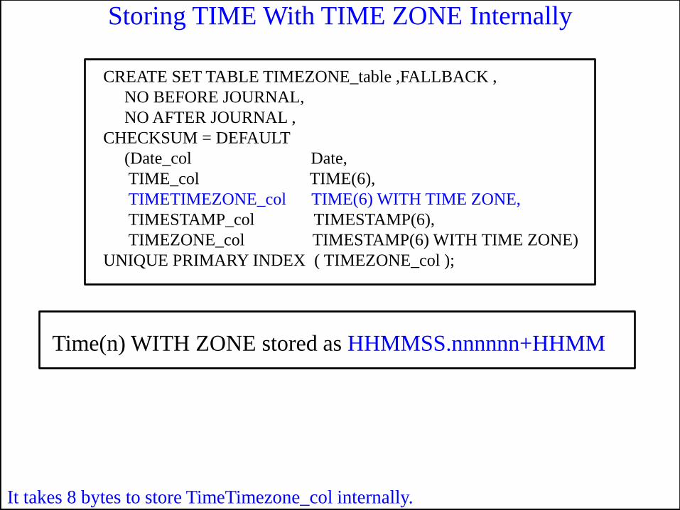
It takes 8 bytes to store TimeTimezone_col internally.
CREATE SET TABLE TIMEZONE_table ,FALLBACK ,
NO BEFORE JOURNAL,
NO AFTER JOURNAL ,
CHECKSUM = DEFAULT
(Date_col Date,
TIME_col TIME(6),
TIMETIMEZONE_col TIME(6) WITH TIME ZONE,
TIMESTAMP_col TIMESTAMP(6),
TIMEZONE_col TIMESTAMP(6) WITH TIME ZONE)
UNIQUE PRIMARY INDEX ( TIMEZONE_col );
Time(n) WITH ZONE stored as HHMMSS.nnnnnn+HHMM
Storing TIME With TIME ZONE Internally
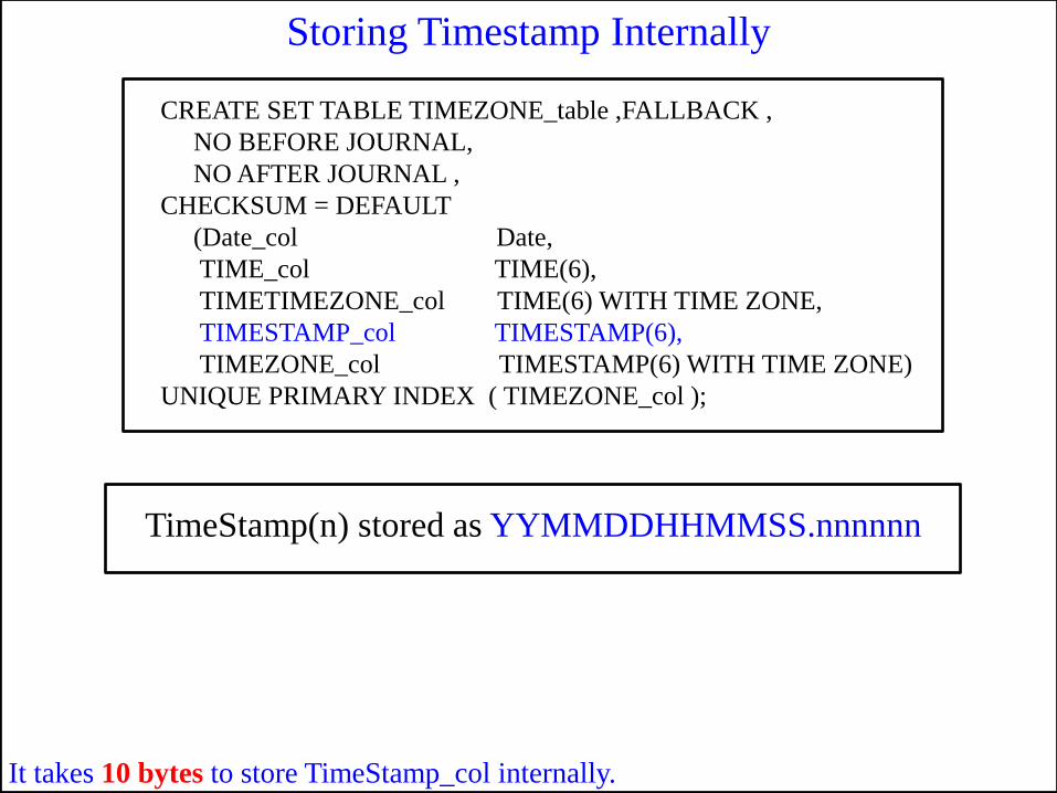
It takes 10 bytes to store TimeStamp_col internally.
Storing Timestamp Internally
CREATE SET TABLE TIMEZONE_table ,FALLBACK ,
NO BEFORE JOURNAL,
NO AFTER JOURNAL ,
CHECKSUM = DEFAULT
(Date_col Date,
TIME_col TIME(6),
TIMETIMEZONE_col TIME(6) WITH TIME ZONE,
TIMESTAMP_col TIMESTAMP(6),
TIMEZONE_col TIMESTAMP(6) WITH TIME ZONE)
UNIQUE PRIMARY INDEX ( TIMEZONE_col );
TimeStamp(n) stored as YYMMDDHHMMSS.nnnnnn
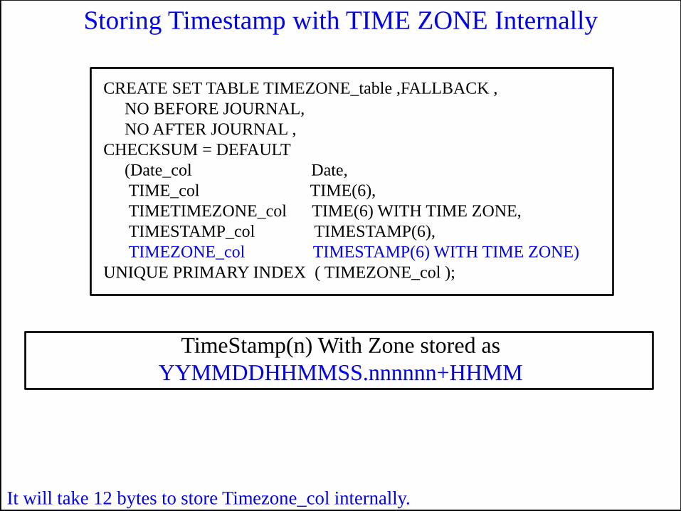
It will take 12 bytes to store Timezone_col internally.
Storing Timestamp with TIME ZONE Internally
CREATE SET TABLE TIMEZONE_table ,FALLBACK ,
NO BEFORE JOURNAL,
NO AFTER JOURNAL ,
CHECKSUM = DEFAULT
(Date_col Date,
TIME_col TIME(6),
TIMETIMEZONE_col TIME(6) WITH TIME ZONE,
TIMESTAMP_col TIMESTAMP(6),
TIMEZONE_col TIMESTAMP(6) WITH TIME ZONE)
UNIQUE PRIMARY INDEX ( TIMEZONE_col );
TimeStamp(n) With Zone stored as
YYMMDDHHMMSS.nnnnnn+HHMM
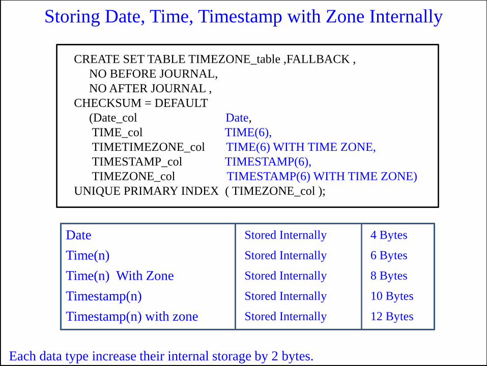
Each data type increase their internal storage by 2 bytes.
Storing Date, Time, Timestamp with Zone Internally
CREATE SET TABLE TIMEZONE_table ,FALLBACK ,
NO BEFORE JOURNAL,
NO AFTER JOURNAL ,
CHECKSUM = DEFAULT
(Date_col Date,
TIME_col TIME(6),
TIMETIMEZONE_col TIME(6) WITH TIME ZONE,
TIMESTAMP_col TIMESTAMP(6),
TIMEZONE_col TIMESTAMP(6) WITH TIME ZONE)
UNIQUE PRIMARY INDEX ( TIMEZONE_col );
Date
Time(n)
Time(n) With Zone
Timestamp(n)
Timestamp(n) with zone
Stored Internally
Stored Internally
Stored Internally
Stored Internally
Stored Internally
4 Bytes
6 Bytes
8 Bytes
10 Bytes
12 Bytes
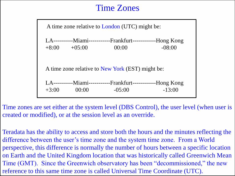
Teradata has the ability to access and store both the hours and the minutes reflecting the
difference between the user‟s time zone and the system time zone. From a World
perspective, this difference is normally the number of hours between a specific location
on Earth and the United Kingdom location that was historically called Greenwich Mean
Time (GMT). Since the Greenwich observatory has been “decommissioned,” the new
reference to this same time zone is called Universal Time Coordinate (UTC).
Time Zones
A time zone relative to London (UTC) might be:
LA----------Miami-----------Frankfurt------------Hong Kong
+8:00 +05:00 00:00 -08:00
A time zone relative to New York (EST) might be:
LA----------Miami-----------Frankfurt------------Hong Kong
+3:00 00:00 -05:00 -13:00
Time zones are set either at the system level (DBS Control), the user level (when user is
created or modified), or at the session level as an override.
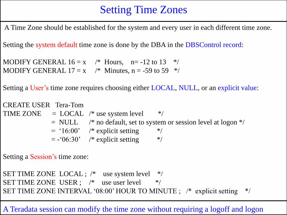
Setting Time Zones
A Time Zone should be established for the system and every user in each different time zone.
Setting the system default time zone is done by the DBA in the DBSControl record:
MODIFY GENERAL 16 = x /* Hours, n= -12 to 13 */
MODIFY GENERAL 17 = x /* Minutes, n = -59 to 59 */
Setting a User‟s time zone requires choosing either LOCAL, NULL, or an explicit value:
CREATE USER Tera-Tom
TIME ZONE = LOCAL /* use system level */
= NULL /* no default, set to system or session level at logon */
= „16:00‟ /* explicit setting */
= -„06:30‟ /* explicit setting */
Setting a Session‟s time zone:
SET TIME ZONE LOCAL ; /* use system level */
SET TIME ZONE USER ; /* use user level */
SET TIME ZONE INTERVAL „08:00‟ HOUR TO MINUTE ; /* explicit setting */
A Teradata session can modify the time zone without requiring a logoff and logon
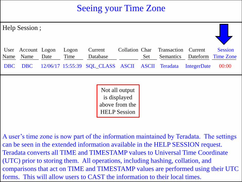
Seeing your Time Zone
DBC DBC 12/06/17 15:55:39 SQL_CLASS ASCII ASCII Teradata IntegerDate 00:00
A user‟s time zone is now part of the information maintained by Teradata. The settings
can be seen in the extended information available in the HELP SESSION request.
Teradata converts all TIME and TIMESTAMP values to Universal Time Coordinate
(UTC) prior to storing them. All operations, including hashing, collation, and
comparisons that act on TIME and TIMESTAMP values are performed using their UTC
forms. This will allow users to CAST the information to their local times.
User Account Logon Logon Current Collation Char Transaction Current Session
Name Name Date Time Database Set Semantics Dateform Time Zone _____ _______ _______ _______ ___________ _______ ______ _________ ________ _________
Help Session ;
Not all output
is displayed
above from the
HELP Session
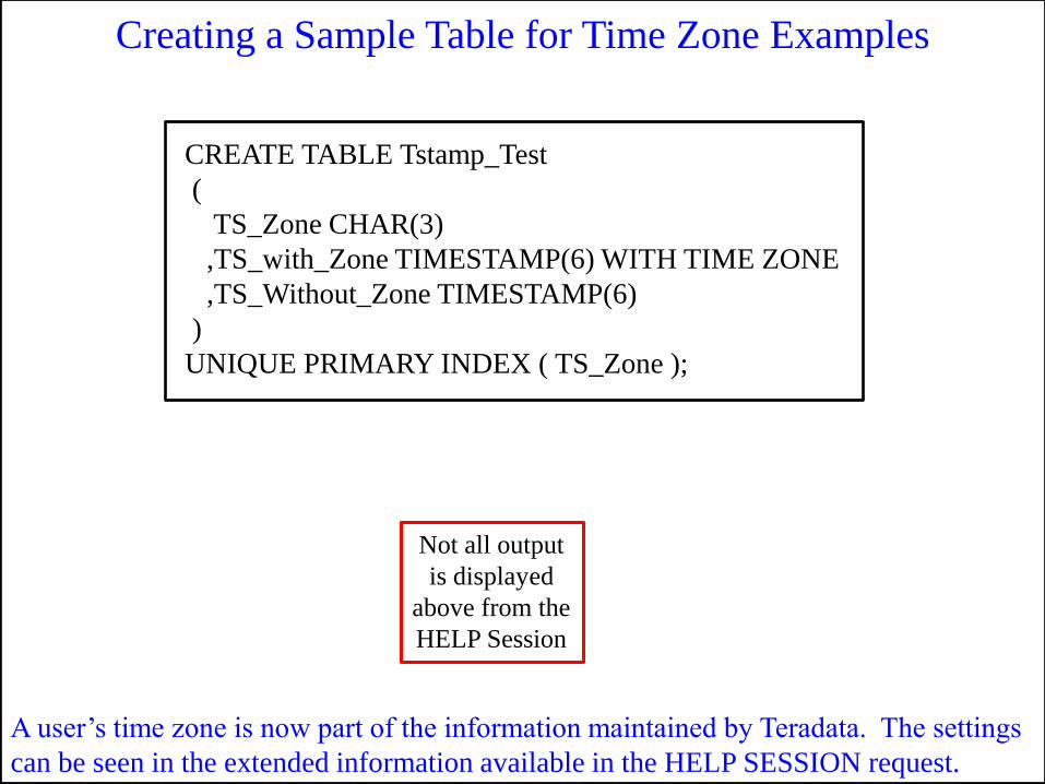
Creating a Sample Table for Time Zone Examples
A user‟s time zone is now part of the information maintained by Teradata. The settings
can be seen in the extended information available in the HELP SESSION request.
CREATE TABLE Tstamp_Test
(
TS_Zone CHAR(3)
,TS_with_Zone TIMESTAMP(6) WITH TIME ZONE
,TS_Without_Zone TIMESTAMP(6)
)
UNIQUE PRIMARY INDEX ( TS_Zone );
Not all output
is displayed
above from the
HELP Session
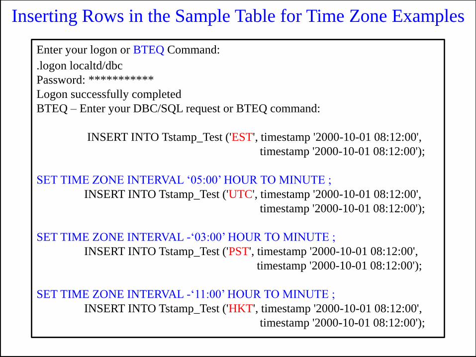
Inserting Rows in the Sample Table for Time Zone Examples
Enter your logon or BTEQ Command:
.logon localtd/dbc
Password: ***********
Logon successfully completed
BTEQ – Enter your DBC/SQL request or BTEQ command:
INSERT INTO Tstamp_Test ('EST', timestamp '2000-10-01 08:12:00',
timestamp '2000-10-01 08:12:00');
SET TIME ZONE INTERVAL „05:00‟ HOUR TO MINUTE ;
INSERT INTO Tstamp_Test ('UTC', timestamp '2000-10-01 08:12:00',
timestamp '2000-10-01 08:12:00');
SET TIME ZONE INTERVAL -„03:00‟ HOUR TO MINUTE ;
INSERT INTO Tstamp_Test ('PST', timestamp '2000-10-01 08:12:00',
timestamp '2000-10-01 08:12:00');
SET TIME ZONE INTERVAL -„11:00‟ HOUR TO MINUTE ;
INSERT INTO Tstamp_Test ('HKT', timestamp '2000-10-01 08:12:00',
timestamp '2000-10-01 08:12:00');
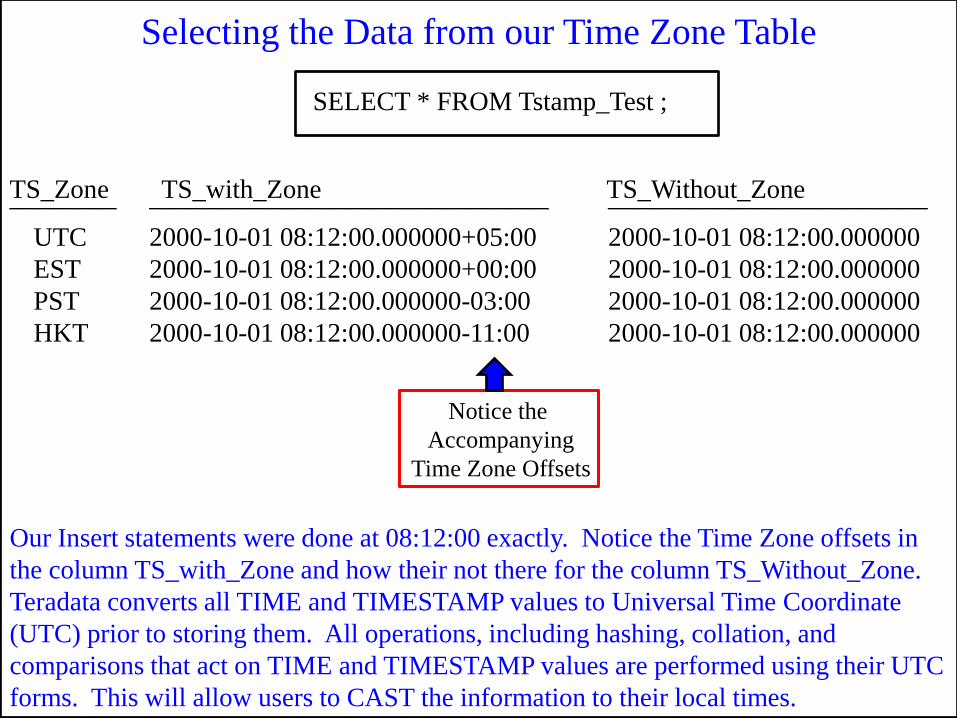
Selecting the Data from our Time Zone Table
Our Insert statements were done at 08:12:00 exactly. Notice the Time Zone offsets in
the column TS_with_Zone and how their not there for the column TS_Without_Zone.
Teradata converts all TIME and TIMESTAMP values to Universal Time Coordinate
(UTC) prior to storing them. All operations, including hashing, collation, and
comparisons that act on TIME and TIMESTAMP values are performed using their UTC
forms. This will allow users to CAST the information to their local times.
SELECT * FROM Tstamp_Test ;
UTC 2000-10-01 08:12:00.000000+05:00 2000-10-01 08:12:00.000000
EST 2000-10-01 08:12:00.000000+00:00 2000-10-01 08:12:00.000000
PST 2000-10-01 08:12:00.000000-03:00 2000-10-01 08:12:00.000000
HKT 2000-10-01 08:12:00.000000-11:00 2000-10-01 08:12:00.000000
TS_Zone TS_with_Zone TS_Without_Zone ________ ______________________________ ________________________
Notice the
Accompanying
Time Zone Offsets
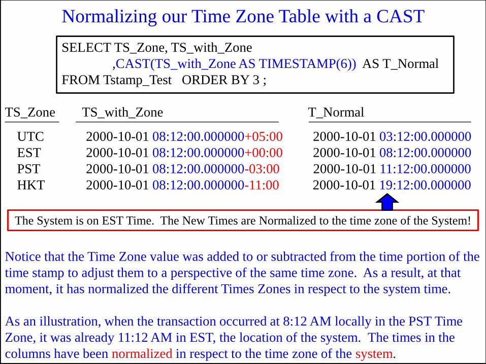
SELECT TS_Zone, TS_with_Zone
,CAST(TS_with_Zone AS TIMESTAMP(6)) AS T_Normal
FROM Tstamp_Test ORDER BY 3 ;
Normalizing our Time Zone Table with a CAST
Notice that the Time Zone value was added to or subtracted from the time portion of the
time stamp to adjust them to a perspective of the same time zone. As a result, at that
moment, it has normalized the different Times Zones in respect to the system time.
As an illustration, when the transaction occurred at 8:12 AM locally in the PST Time
Zone, it was already 11:12 AM in EST, the location of the system. The times in the
columns have been normalized in respect to the time zone of the system.
UTC 2000-10-01 08:12:00.000000+05:00 2000-10-01 03:12:00.000000
EST 2000-10-01 08:12:00.000000+00:00 2000-10-01 08:12:00.000000
PST 2000-10-01 08:12:00.000000-03:00 2000-10-01 11:12:00.000000
HKT 2000-10-01 08:12:00.000000-11:00 2000-10-01 19:12:00.000000
TS_Zone TS_with_Zone T_Normal ________ ______________________________ ________________________
The System is on EST Time. The New Times are Normalized to the time zone of the System!
Intervals for Date, Time and Timestamp
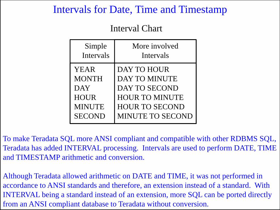
To make Teradata SQL more ANSI compliant and compatible with other RDBMS SQL,
Teradata has added INTERVAL processing. Intervals are used to perform DATE, TIME
and TIMESTAMP arithmetic and conversion.
Although Teradata allowed arithmetic on DATE and TIME, it was not performed in
accordance to ANSI standards and therefore, an extension instead of a standard. With
INTERVAL being a standard instead of an extension, more SQL can be ported directly
from an ANSI compliant database to Teradata without conversion.
YEAR
MONTH
DAY
HOUR
MINUTE
SECOND
DAY TO HOUR
DAY TO MINUTE
DAY TO SECOND
HOUR TO MINUTE
HOUR TO SECOND
MINUTE TO SECOND
Simple
Intervals
More involved
Intervals
Interval Chart
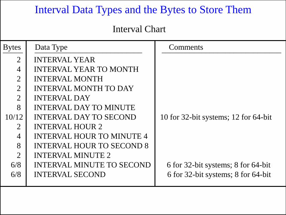
Interval Data Types and the Bytes to Store Them
Interval Chart
Bytes Data Type Comments
INTERVAL YEAR
INTERVAL YEAR TO MONTH
INTERVAL MONTH
INTERVAL MONTH TO DAY
INTERVAL DAY
INTERVAL DAY TO MINUTE
INTERVAL DAY TO SECOND 10 for 32-bit systems; 12 for 64-bit
INTERVAL HOUR 2
INTERVAL HOUR TO MINUTE 4
INTERVAL HOUR TO SECOND 8
INTERVAL MINUTE 2
INTERVAL MINUTE TO SECOND 6 for 32-bit systems; 8 for 64-bit
INTERVAL SECOND 6 for 32-bit systems; 8 for 64-bit
2
4
2
2
2
8
10/12
2
4
8
2
6/8
6/8
_____ ___________________________ ______________________________
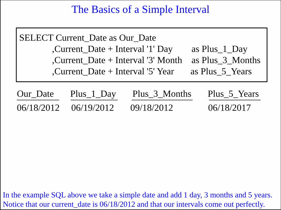
The Basics of a Simple Interval
In the example SQL above we take a simple date and add 1 day, 3 months and 5 years.
Notice that our current_date is 06/18/2012 and that our intervals come out perfectly.
SELECT Current_Date as Our_Date
,Current_Date + Interval '1' Day as Plus_1_Day
,Current_Date + Interval '3' Month as Plus_3_Months
,Current_Date + Interval '5' Year as Plus_5_Years
Our_Date Plus_1_Day Plus_3_Months Plus_5_Years _________ __________ _____________ ___________
06/18/2012 06/19/2012 09/18/2012 06/18/2017
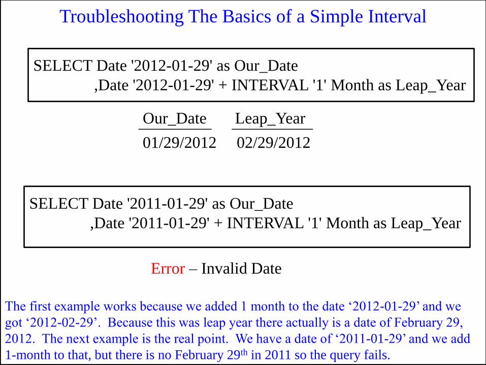
Troubleshooting The Basics of a Simple Interval
The first example works because we added 1 month to the date „2012-01-29‟ and we
got „2012-02-29‟. Because this was leap year there actually is a date of February 29,
2012. The next example is the real point. We have a date of „2011-01-29‟ and we add
1-month to that, but there is no February 29th in 2011 so the query fails.
SELECT Date '2012-01-29' as Our_Date
,Date '2012-01-29' + INTERVAL '1' Month as Leap_Year
Our_Date Leap_Year _________ __________
01/29/2012 02/29/2012
SELECT Date '2011-01-29' as Our_Date
,Date '2011-01-29' + INTERVAL '1' Month as Leap_Year
Error – Invalid Date
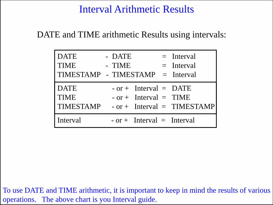
Interval Arithmetic Results
To use DATE and TIME arithmetic, it is important to keep in mind the results of various
operations. The above chart is you Interval guide.
DATE - DATE = Interval
TIME - TIME = Interval
TIMESTAMP - TIMESTAMP = Interval
DATE and TIME arithmetic Results using intervals:
DATE - or + Interval = DATE
TIME - or + Interval = TIME
TIMESTAMP - or + Interval = TIMESTAMP
Interval - or + Interval = Interval
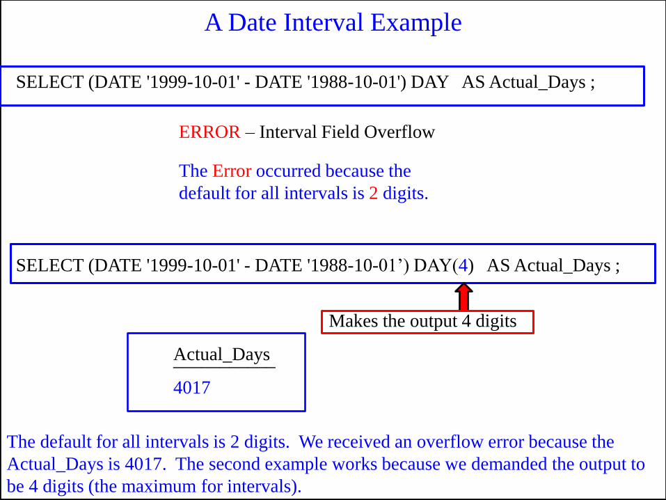
A Date Interval Example
The default for all intervals is 2 digits. We received an overflow error because the
Actual_Days is 4017. The second example works because we demanded the output to
be 4 digits (the maximum for intervals).
SELECT (DATE '1999-10-01' - DATE '1988-10-01‟) DAY(4) AS Actual_Days ;
Actual_Days
4017
___________
Makes the output 4 digits
SELECT (DATE '1999-10-01' - DATE '1988-10-01') DAY AS Actual_Days ;
ERROR – Interval Field Overflow
The Error occurred because the
default for all intervals is 2 digits.
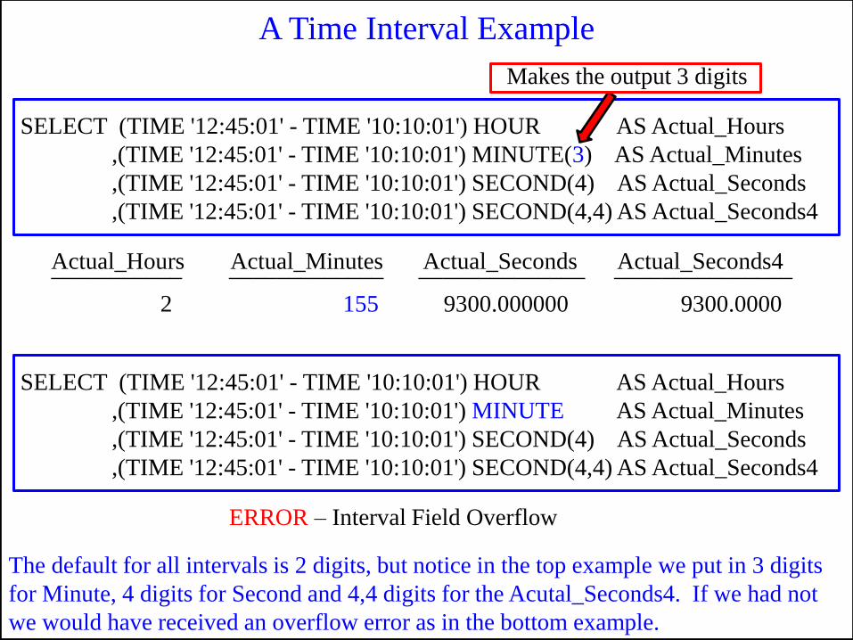
A Time Interval Example
The default for all intervals is 2 digits, but notice in the top example we put in 3 digits
for Minute, 4 digits for Second and 4,4 digits for the Acutal_Seconds4. If we had not
we would have received an overflow error as in the bottom example.
SELECT (TIME '12:45:01' - TIME '10:10:01') HOUR AS Actual_Hours
,(TIME '12:45:01' - TIME '10:10:01') MINUTE(3) AS Actual_Minutes
,(TIME '12:45:01' - TIME '10:10:01') SECOND(4) AS Actual_Seconds
,(TIME '12:45:01' - TIME '10:10:01') SECOND(4,4) AS Actual_Seconds4
Actual_Hours Actual_Minutes Actual_Seconds Actual_Seconds4
2 155 9300.000000 9300.0000
___________ _____________ ______________ _______________
Makes the output 3 digits
SELECT (TIME '12:45:01' - TIME '10:10:01') HOUR AS Actual_Hours
,(TIME '12:45:01' - TIME '10:10:01') MINUTE AS Actual_Minutes
,(TIME '12:45:01' - TIME '10:10:01') SECOND(4) AS Actual_Seconds
,(TIME '12:45:01' - TIME '10:10:01') SECOND(4,4) AS Actual_Seconds4
ERROR – Interval Field Overflow
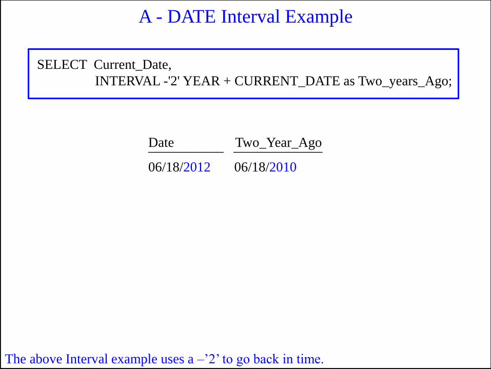
A - DATE Interval Example
The above Interval example uses a –‟2‟ to go back in time.
SELECT Current_Date,
INTERVAL -'2' YEAR + CURRENT_DATE as Two_years_Ago;
Date Two_Year_Ago
06/18/2012 06/18/2010
___________ _____________
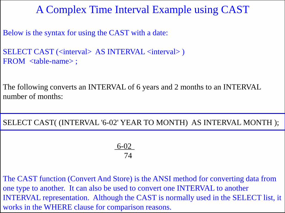
A Complex Time Interval Example using CAST
The CAST function (Convert And Store) is the ANSI method for converting data from
one type to another. It can also be used to convert one INTERVAL to another
INTERVAL representation. Although the CAST is normally used in the SELECT list, it
works in the WHERE clause for comparison reasons.
SELECT CAST( (INTERVAL '6-02' YEAR TO MONTH) AS INTERVAL MONTH );
74
6-02
The following converts an INTERVAL of 6 years and 2 months to an INTERVAL
number of months:
_____
Below is the syntax for using the CAST with a date:
SELECT CAST (<interval> AS INTERVAL <interval> )
FROM <table-name> ;
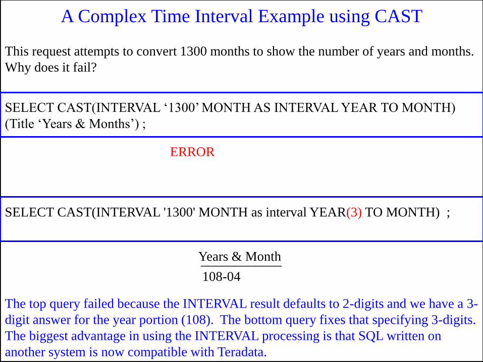
A Complex Time Interval Example using CAST
The top query failed because the INTERVAL result defaults to 2-digits and we have a 3-
digit answer for the year portion (108). The bottom query fixes that specifying 3-digits.
The biggest advantage in using the INTERVAL processing is that SQL written on
another system is now compatible with Teradata.
SELECT CAST(INTERVAL „1300‟ MONTH AS INTERVAL YEAR TO MONTH)
(Title „Years & Months‟) ;
108-04
Years & Month
This request attempts to convert 1300 months to show the number of years and months.
Why does it fail?
____________
SELECT CAST(INTERVAL '1300' MONTH as interval YEAR(3) TO MONTH) ;
ERROR
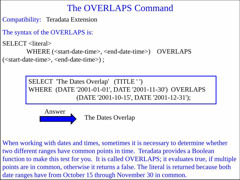
The OVERLAPS Command
When working with dates and times, sometimes it is necessary to determine whether
two different ranges have common points in time. Teradata provides a Boolean
function to make this test for you. It is called OVERLAPS; it evaluates true, if multiple
points are in common, otherwise it returns a false. The literal is returned because both
date ranges have from October 15 through November 30 in common.
The Dates Overlap
Compatibility: Teradata Extension
The syntax of the OVERLAPS is:
SELECT <literal>
WHERE (<start-date-time>, <end-date-time>) OVERLAPS
(<start-date-time>, <end-date-time>) ;
SELECT 'The Dates Overlap' (TITLE ' ')
WHERE (DATE '2001-01-01', DATE '2001-11-30') OVERLAPS
(DATE '2001-10-15', DATE '2001-12-31');
Answer
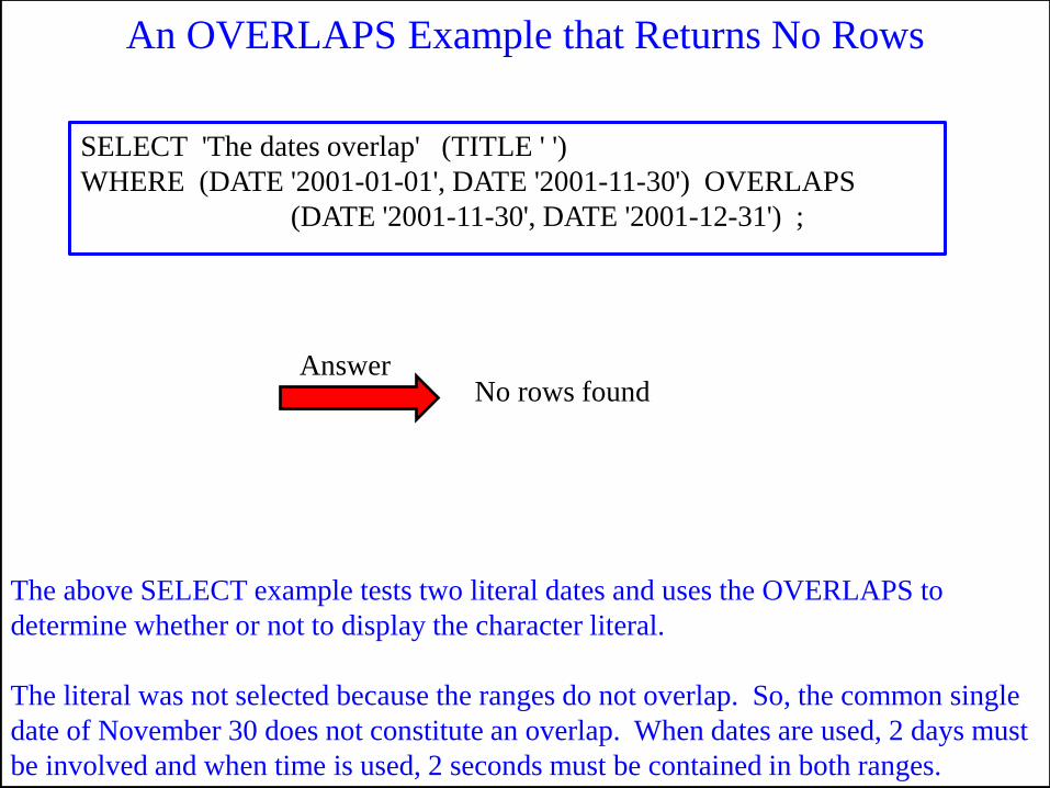
An OVERLAPS Example that Returns No Rows
The above SELECT example tests two literal dates and uses the OVERLAPS to
determine whether or not to display the character literal.
The literal was not selected because the ranges do not overlap. So, the common single
date of November 30 does not constitute an overlap. When dates are used, 2 days must
be involved and when time is used, 2 seconds must be contained in both ranges.
No rows found
SELECT 'The dates overlap' (TITLE ' ')
WHERE (DATE '2001-01-01', DATE '2001-11-30') OVERLAPS
(DATE '2001-11-30', DATE '2001-12-31') ;
Answer
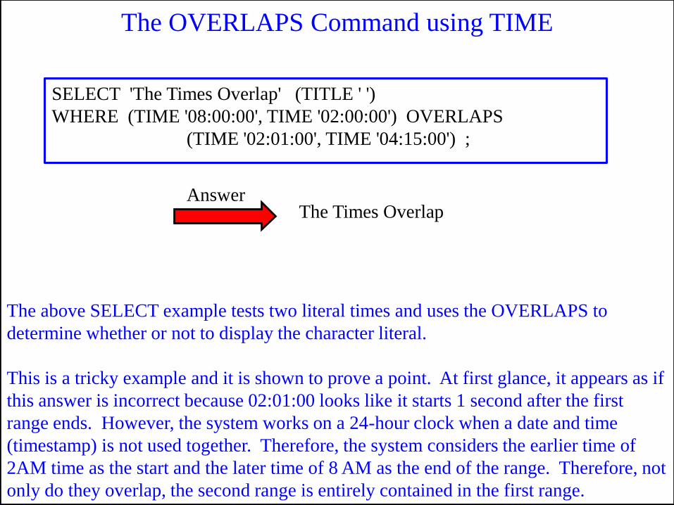
The OVERLAPS Command using TIME
The above SELECT example tests two literal times and uses the OVERLAPS to
determine whether or not to display the character literal.
This is a tricky example and it is shown to prove a point. At first glance, it appears as if
this answer is incorrect because 02:01:00 looks like it starts 1 second after the first
range ends. However, the system works on a 24-hour clock when a date and time
(timestamp) is not used together. Therefore, the system considers the earlier time of
2AM time as the start and the later time of 8 AM as the end of the range. Therefore, not
only do they overlap, the second range is entirely contained in the first range.
The Times Overlap
SELECT 'The Times Overlap' (TITLE ' ')
WHERE (TIME '08:00:00', TIME '02:00:00') OVERLAPS
(TIME '02:01:00', TIME '04:15:00') ;
Answer
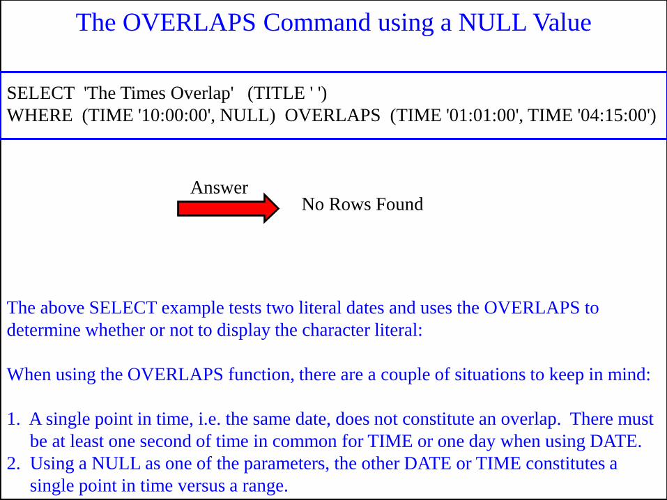
The OVERLAPS Command using a NULL Value
The above SELECT example tests two literal dates and uses the OVERLAPS to
determine whether or not to display the character literal:
When using the OVERLAPS function, there are a couple of situations to keep in mind:
1. A single point in time, i.e. the same date, does not constitute an overlap. There must
be at least one second of time in common for TIME or one day when using DATE.
2. Using a NULL as one of the parameters, the other DATE or TIME constitutes a
single point in time versus a range.
No Rows Found
SELECT 'The Times Overlap' (TITLE ' ')
WHERE (TIME '10:00:00', NULL) OVERLAPS (TIME '01:01:00', TIME '04:15:00')
Answer

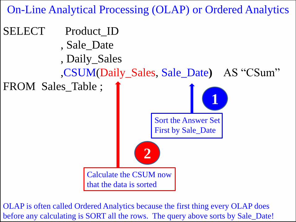
OLAP is often called Ordered Analytics because the first thing every OLAP does
before any calculating is SORT all the rows. The query above sorts by Sale_Date!
SELECT Product_ID
, Sale_Date
, Daily_Sales
,CSUM(Daily_Sales, Sale_Date) AS “CSum”
FROM Sales_Table ;
On-Line Analytical Processing (OLAP) or Ordered Analytics
Sort the Answer Set
First by Sale_Date
1
Calculate the CSUM now
that the data is sorted
2
OLAP always sorts first and then is in a position to calculate starting with the first
sorted row and continuing to the last sorted row, thus calculating all Daily_Sales.
SELECT Product_ID , Sale_Date, Daily_Sales
,CSUM(Daily_Sales, Sale_Date) AS “CSum”
FROM Sales_Table ;
Sort the Answer Set
first by Sale_Date, but
Don‟t do any CSUM
Calculations yet!
1
Product_ID Sale_Date Daily_Sales CSUM
1000
2000
3000
1000
2000
3000
1000
2000
3000
1000
2000
3000
1000
2000
3000
2000-09-28
2000-09-28
2000-09-28
2000-09-29
2000-09-29
2000-09-29
2000-09-30
2000-09-30
2000-09-30
2000-10-01
2000-10-01
2000-10-01
2000-10-02
2000-10-02
2000-10-02
48850.40
41888.88
61301.77
54500.22
48000.00
34509.13
36000.07
49850.03
43868.86
40200.43
54850.29
28000.00
32800.50
36021.93
19678.94
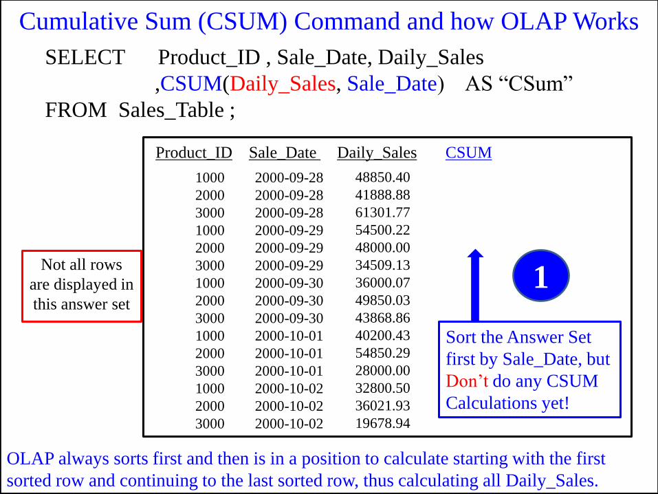
Cumulative Sum (CSUM) Command and how OLAP Works
Not all rows
are displayed in
this answer set
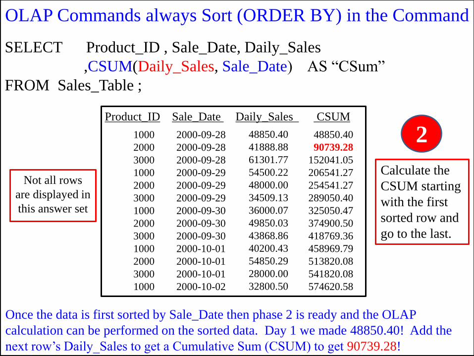
Once the data is first sorted by Sale_Date then phase 2 is ready and the OLAP
calculation can be performed on the sorted data. Day 1 we made 48850.40! Add the
next row‟s Daily_Sales to get a Cumulative Sum (CSUM) to get 90739.28!
SELECT Product_ID , Sale_Date, Daily_Sales
,CSUM(Daily_Sales, Sale_Date) AS “CSum”
FROM Sales_Table ;
Calculate the
CSUM starting
with the first
sorted row and
go to the last.
2 Product_ID Sale_Date Daily_Sales CSUM
1000
2000
3000
1000
2000
3000
1000
2000
3000
1000
2000
3000
1000
2000-09-28
2000-09-28
2000-09-28
2000-09-29
2000-09-29
2000-09-29
2000-09-30
2000-09-30
2000-09-30
2000-10-01
2000-10-01
2000-10-01
2000-10-02
48850.40
41888.88
61301.77
54500.22
48000.00
34509.13
36000.07
49850.03
43868.86
40200.43
54850.29
28000.00
32800.50
48850.40
90739.28
152041.05
206541.27
254541.27
289050.40
325050.47
374900.50
418769.36
458969.79
513820.08
541820.08
574620.58
OLAP Commands always Sort (ORDER BY) in the Command
Not all rows
are displayed in
this answer set
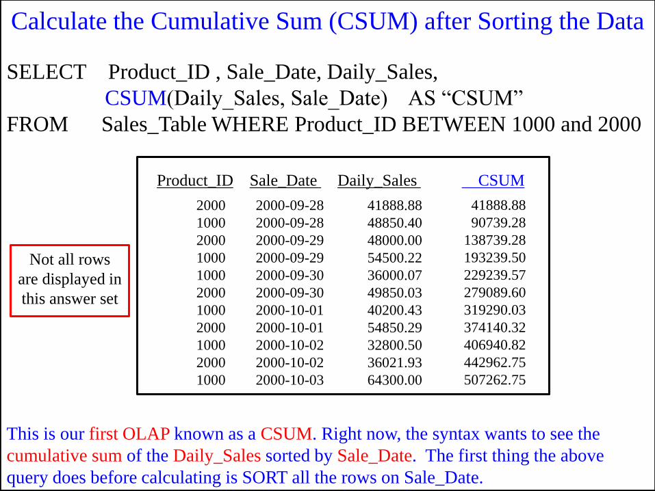
This is our first OLAP known as a CSUM. Right now, the syntax wants to see the
cumulative sum of the Daily_Sales sorted by Sale_Date. The first thing the above
query does before calculating is SORT all the rows on Sale_Date.
SELECT Product_ID , Sale_Date, Daily_Sales,
CSUM(Daily_Sales, Sale_Date) AS “CSUM”
FROM Sales_Table WHERE Product_ID BETWEEN 1000 and 2000
Product_ID Sale_Date Daily_Sales CSUM
2000
1000
2000
1000
1000
2000
1000
2000
1000
2000
1000
2000-09-28
2000-09-28
2000-09-29
2000-09-29
2000-09-30
2000-09-30
2000-10-01
2000-10-01
2000-10-02
2000-10-02
2000-10-03
41888.88
48850.40
48000.00
54500.22
36000.07
49850.03
40200.43
54850.29
32800.50
36021.93
64300.00
41888.88
90739.28
138739.28
193239.50
229239.57
279089.60
319290.03
374140.32
406940.82
442962.75
507262.75
Calculate the Cumulative Sum (CSUM) after Sorting the Data
Not all rows
are displayed in
this answer set
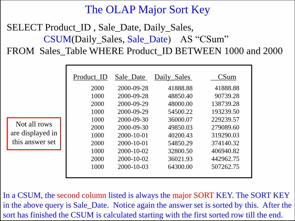
In a CSUM, the second column listed is always the major SORT KEY. The SORT KEY
in the above query is Sale_Date. Notice again the answer set is sorted by this. After the
sort has finished the CSUM is calculated starting with the first sorted row till the end.
SELECT Product_ID , Sale_Date, Daily_Sales,
CSUM(Daily_Sales, Sale_Date) AS “CSum”
FROM Sales_Table WHERE Product_ID BETWEEN 1000 and 2000
Product_ID Sale_Date Daily_Sales CSum
2000
1000
2000
1000
1000
2000
1000
2000
1000
2000
1000
2000-09-28
2000-09-28
2000-09-29
2000-09-29
2000-09-30
2000-09-30
2000-10-01
2000-10-01
2000-10-02
2000-10-02
2000-10-03
41888.88
48850.40
48000.00
54500.22
36000.07
49850.03
40200.43
54850.29
32800.50
36021.93
64300.00
41888.88
90739.28
138739.28
193239.50
229239.57
279089.60
319290.03
374140.32
406940.82
442962.75
507262.75
The OLAP Major Sort Key
Not all rows
are displayed in
this answer set
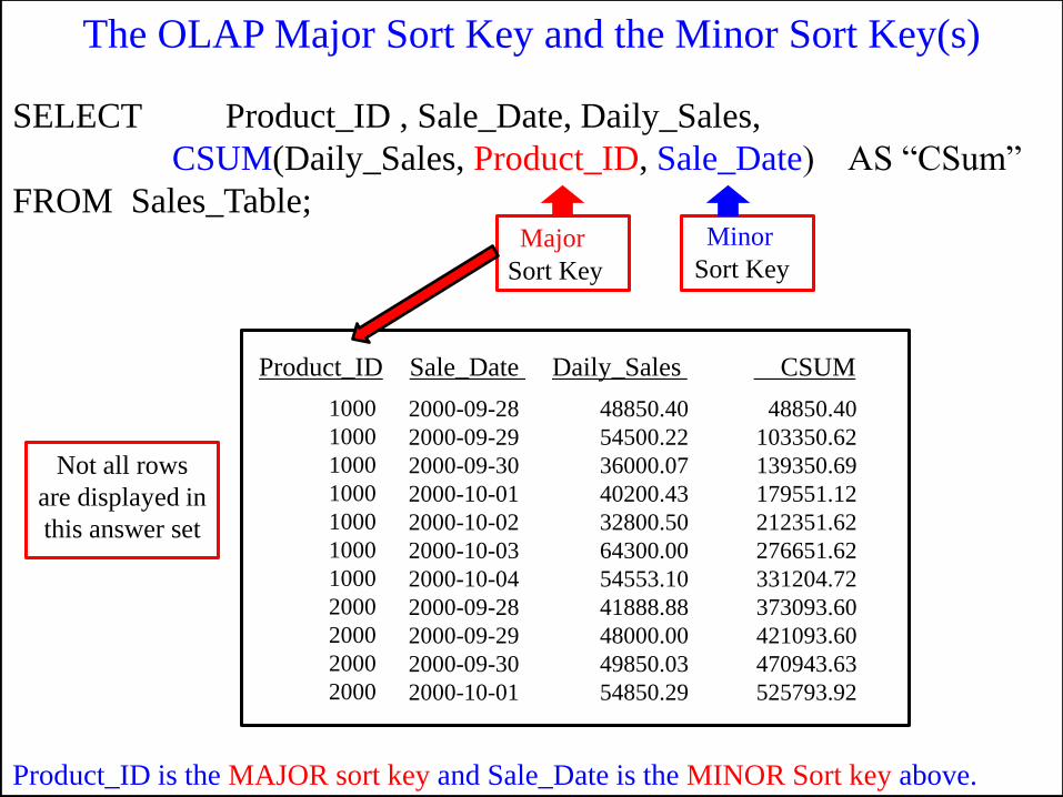
Product_ID is the MAJOR sort key and Sale_Date is the MINOR Sort key above.
SELECT Product_ID , Sale_Date, Daily_Sales,
CSUM(Daily_Sales, Product_ID, Sale_Date) AS “CSum”
FROM Sales_Table;
Product_ID Sale_Date Daily_Sales CSUM
1000
1000
1000
1000
1000
1000
1000
2000
2000
2000
2000
2000-09-28
2000-09-29
2000-09-30
2000-10-01
2000-10-02
2000-10-03
2000-10-04
2000-09-28
2000-09-29
2000-09-30
2000-10-01
48850.40
54500.22
36000.07
40200.43
32800.50
64300.00
54553.10
41888.88
48000.00
49850.03
54850.29
48850.40
103350.62
139350.69
179551.12
212351.62
276651.62
331204.72
373093.60
421093.60
470943.63
525793.92
Major
Sort Key
Minor
Sort Key
The OLAP Major Sort Key and the Minor Sort Key(s)
Not all rows
are displayed in
this answer set
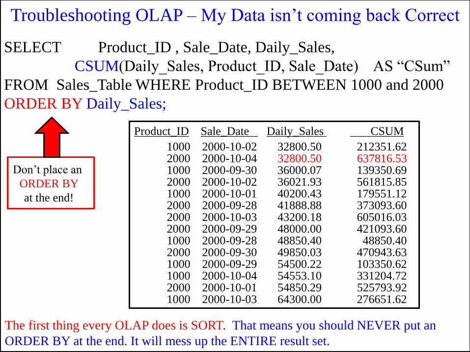
The first thing every OLAP does is SORT. That means you should NEVER put an
ORDER BY at the end. It will mess up the ENTIRE result set.
SELECT Product_ID , Sale_Date, Daily_Sales,
CSUM(Daily_Sales, Product_ID, Sale_Date) AS “CSum”
FROM Sales_Table WHERE Product_ID BETWEEN 1000 and 2000
ORDER BY Daily_Sales;
Product_ID Sale_Date Daily_Sales CSUM
1000 2000-10-02 32800.50 212351.62 2000 2000-10-04 32800.50 637816.53 1000 2000-09-30 36000.07 139350.69 2000 2000-10-02 36021.93 561815.85 1000 2000-10-01 40200.43 179551.12 2000 2000-09-28 41888.88 373093.60 2000 2000-10-03 43200.18 605016.03 2000 2000-09-29 48000.00 421093.60 1000 2000-09-28 48850.40 48850.40 2000 2000-09-30 49850.03 470943.63 1000 2000-09-29 54500.22 103350.62 1000 2000-10-04 54553.10 331204.72 2000 2000-10-01 54850.29 525793.92 1000 2000-10-03 64300.00 276651.62
Don‟t place an
ORDER BY
at the end!
Troubleshooting OLAP – My Data isn‟t coming back Correct
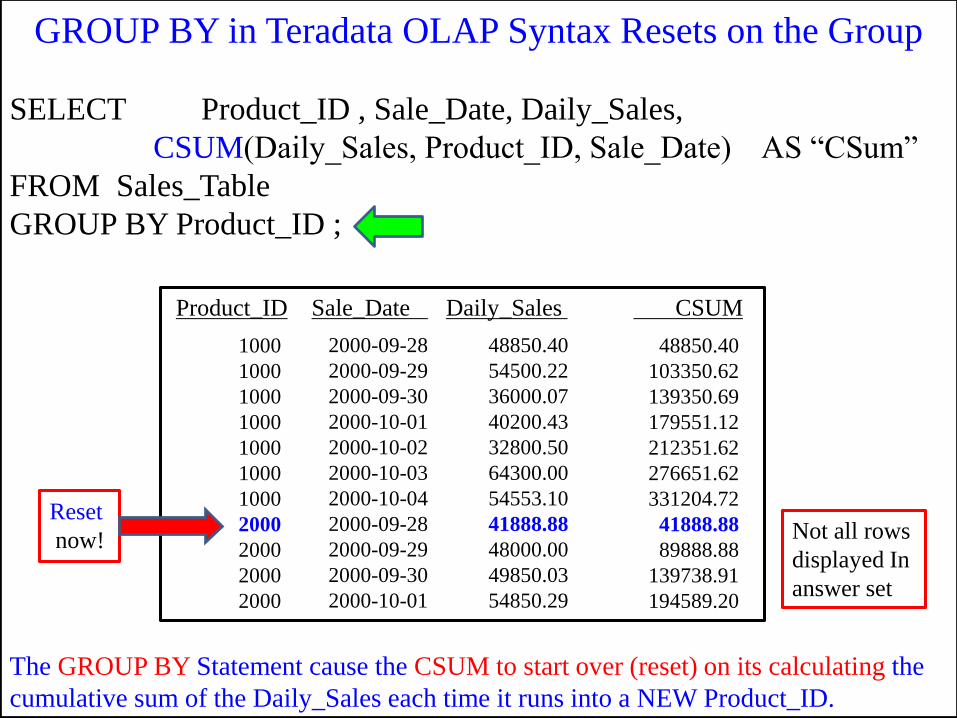
The GROUP BY Statement cause the CSUM to start over (reset) on its calculating the
cumulative sum of the Daily_Sales each time it runs into a NEW Product_ID.
SELECT Product_ID , Sale_Date, Daily_Sales,
CSUM(Daily_Sales, Product_ID, Sale_Date) AS “CSum”
FROM Sales_Table
GROUP BY Product_ID ;
Product_ID Sale_Date Daily_Sales CSUM
1000
1000
1000
1000
1000
1000
1000
2000
2000
2000
2000
2000-09-28
2000-09-29
2000-09-30
2000-10-01
2000-10-02
2000-10-03
2000-10-04
2000-09-28
2000-09-29
2000-09-30
2000-10-01
48850.40
54500.22
36000.07
40200.43
32800.50
64300.00
54553.10
41888.88
48000.00
49850.03
54850.29
48850.40
103350.62
139350.69
179551.12
212351.62
276651.62
331204.72
41888.88
89888.88
139738.91
194589.20
Reset
now! Not all rows
displayed In
answer set
GROUP BY in Teradata OLAP Syntax Resets on the Group
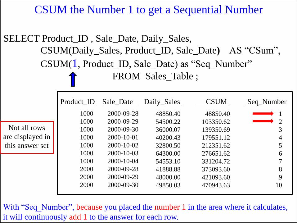
With “Seq_Number”, because you placed the number 1 in the area where it calculates,
it will continuously add 1 to the answer for each row.
SELECT Product_ID , Sale_Date, Daily_Sales,
CSUM(Daily_Sales, Product_ID, Sale_Date) AS “CSum”,
CSUM(1, Product_ID, Sale_Date) as “Seq_Number”
FROM Sales_Table ;
Product_ID Sale_Date Daily_Sales CSUM Seq_Number
1000
1000
1000
1000
1000
1000
1000
2000
2000
2000
2000-09-28
2000-09-29
2000-09-30
2000-10-01
2000-10-02
2000-10-03
2000-10-04
2000-09-28
2000-09-29
2000-09-30
48850.40
54500.22
36000.07
40200.43
32800.50
64300.00
54553.10
41888.88
48000.00
49850.03
48850.40
103350.62
139350.69
179551.12
212351.62
276651.62
331204.72
373093.60
421093.60
470943.63
1
2
3
4
5
6
7
8
9
10
CSUM the Number 1 to get a Sequential Number
Not all rows
are displayed in
this answer set
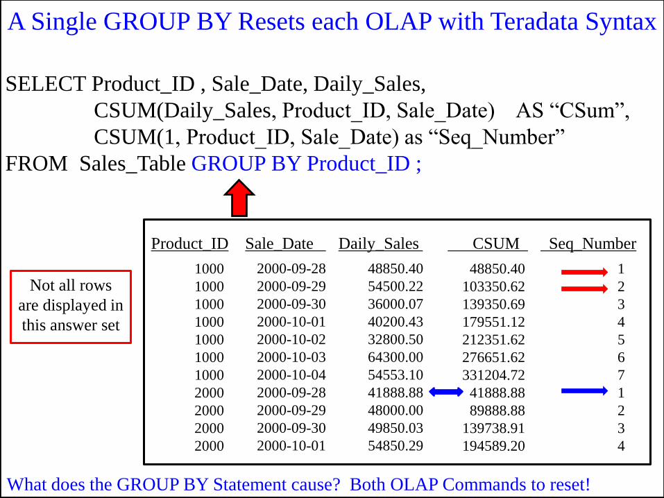
What does the GROUP BY Statement cause? Both OLAP Commands to reset!
SELECT Product_ID , Sale_Date, Daily_Sales,
CSUM(Daily_Sales, Product_ID, Sale_Date) AS “CSum”,
CSUM(1, Product_ID, Sale_Date) as “Seq_Number”
FROM Sales_Table GROUP BY Product_ID ;
1000
1000
1000
1000
1000
1000
1000
2000
2000
2000
2000
2000-09-28
2000-09-29
2000-09-30
2000-10-01
2000-10-02
2000-10-03
2000-10-04
2000-09-28
2000-09-29
2000-09-30
2000-10-01
48850.40
54500.22
36000.07
40200.43
32800.50
64300.00
54553.10
41888.88
48000.00
49850.03
54850.29
48850.40
103350.62
139350.69
179551.12
212351.62
276651.62
331204.72
41888.88
89888.88
139738.91
194589.20
Product_ID Sale_Date Daily_Sales CSUM Seq_Number
1
2
3
4
5
6
7
1
2
3
4
A Single GROUP BY Resets each OLAP with Teradata Syntax
Not all rows
are displayed in
this answer set
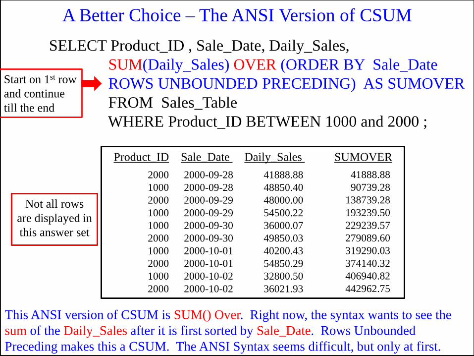
SELECT Product_ID , Sale_Date, Daily_Sales,
SUM(Daily_Sales) OVER (ORDER BY Sale_Date
ROWS UNBOUNDED PRECEDING) AS SUMOVER
FROM Sales_Table
WHERE Product_ID BETWEEN 1000 and 2000 ;
This ANSI version of CSUM is SUM() Over. Right now, the syntax wants to see the
sum of the Daily_Sales after it is first sorted by Sale_Date. Rows Unbounded
Preceding makes this a CSUM. The ANSI Syntax seems difficult, but only at first.
Product_ID Sale_Date Daily_Sales SUMOVER
2000
1000
2000
1000
1000
2000
1000
2000
1000
2000
2000-09-28
2000-09-28
2000-09-29
2000-09-29
2000-09-30
2000-09-30
2000-10-01
2000-10-01
2000-10-02
2000-10-02
41888.88
48850.40
48000.00
54500.22
36000.07
49850.03
40200.43
54850.29
32800.50
36021.93
41888.88
90739.28
138739.28
193239.50
229239.57
279089.60
319290.03
374140.32
406940.82
442962.75
A Better Choice – The ANSI Version of CSUM
Start on 1st row
and continue
till the end
Not all rows
are displayed in
this answer set
SELECT Product_ID , Sale_Date, Daily_Sales,
SUM(Daily_Sales) OVER (ORDER BY Sale_Date
ROWS UNBOUNDED PRECEDING) AS SUMOVER
FROM Sales_Table WHERE Product_ID BETWEEN 1000 and 2000 ;
Product_ID Sale_Date Daily_Sales SUMOVER
2000
1000
2000
1000
1000
2000
1000
2000
1000
2000
1000
2000
2000-09-28
2000-09-28
2000-09-29
2000-09-29
2000-09-30
2000-09-30
2000-10-01
2000-10-01
2000-10-02
2000-10-02
2000-10-03
2000-10-03
41888.88
48850.40
48000.00
54500.22
36000.07
49850.03
40200.43
54850.29
32800.50
36021.93
64300.00
43200.18
41888.88
90739.28
138739.28
193239.50
229239.57
279089.60
319290.03
374140.32
406940.82
442962.75
507262.75
550462.93
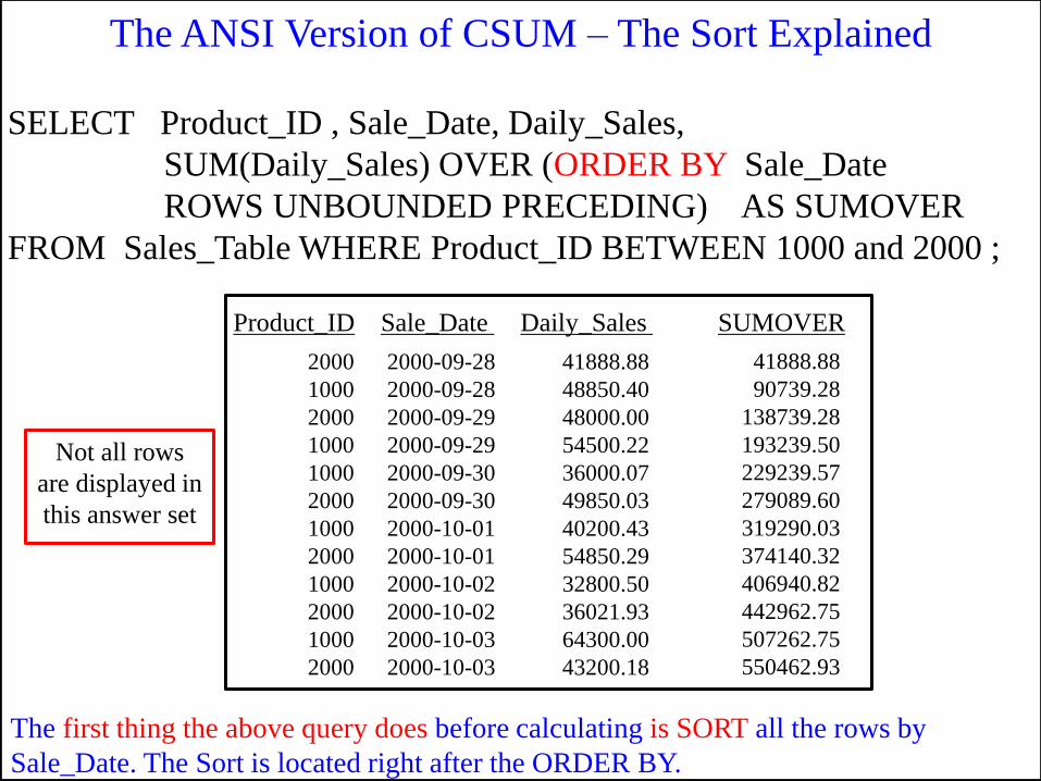
The first thing the above query does before calculating is SORT all the rows by
Sale_Date. The Sort is located right after the ORDER BY.
The ANSI Version of CSUM – The Sort Explained
Not all rows
are displayed in
this answer set
SELECT Product_ID , Sale_Date, Daily_Sales,
SUM(Daily_Sales) OVER (ORDER BY Sale_Date
ROWS UNBOUNDED PRECEDING) AS SUMOVER
FROM Sales_Table WHERE Product_ID BETWEEN 1000 and 2000 ;
Product_ID Sale_Date Daily_Sales SUMOVER
2000
1000
2000
1000
1000
2000
1000
2000
1000
2000
1000
2000-09-28
2000-09-28
2000-09-29
2000-09-29
2000-09-30
2000-09-30
2000-10-01
2000-10-01
2000-10-02
2000-10-02
2000-10-03
41888.88
48850.40
48000.00
54500.22
36000.07
49850.03
40200.43
54850.29
32800.50
36021.93
64300.00
41888.88
90739.28
138739.28
193239.50
229239.57
279089.60
319290.03
374140.32
406940.82
442962.75
507262.75
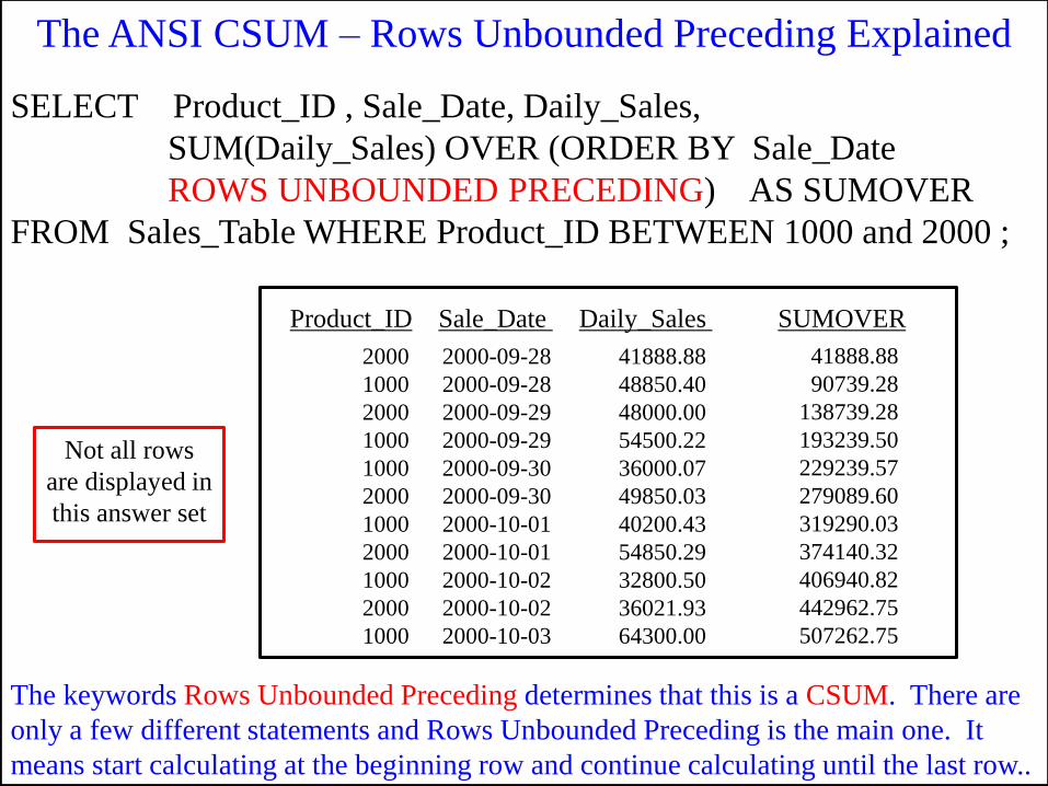
The keywords Rows Unbounded Preceding determines that this is a CSUM. There are
only a few different statements and Rows Unbounded Preceding is the main one. It
means start calculating at the beginning row and continue calculating until the last row..
The ANSI CSUM – Rows Unbounded Preceding Explained
Not all rows
are displayed in
this answer set
SELECT Product_ID , Sale_Date, Daily_Sales,
SUM(Daily_Sales) OVER (ORDER BY Sale_Date
ROWS UNBOUNDED PRECEDING) AS SUMOVER
FROM Sales_Table WHERE Product_ID BETWEEN 1000 and 2000 ;
Product_ID Sale_Date Daily_Sales SUMOVER
2000
1000
2000
1000
1000
2000
1000
2000
1000
2000
1000
2000-09-28
2000-09-28
2000-09-29
2000-09-29
2000-09-30
2000-09-30
2000-10-01
2000-10-01
2000-10-02
2000-10-02
2000-10-03
41888.88
48850.40
48000.00
54500.22
36000.07
49850.03
40200.43
54850.29
32800.50
36021.93
64300.00
41888.88
90739.28
138739.28
193239.50
229239.57
279089.60
319290.03
374140.32
406940.82
442962.75
507262.75
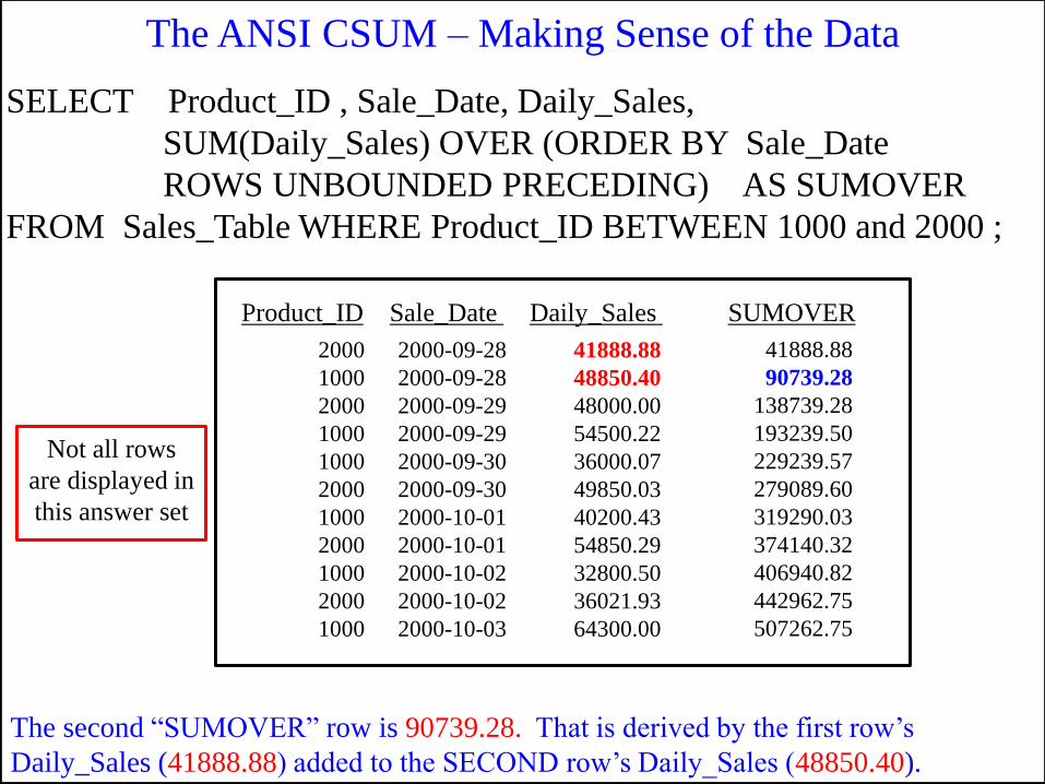
The second “SUMOVER” row is 90739.28. That is derived by the first row‟s
Daily_Sales (41888.88) added to the SECOND row‟s Daily_Sales (48850.40).
The ANSI CSUM – Making Sense of the Data
Not all rows
are displayed in
this answer set
SELECT Product_ID , Sale_Date, Daily_Sales,
SUM(Daily_Sales) OVER (ORDER BY Sale_Date
ROWS UNBOUNDED PRECEDING) AS SUMOVER
FROM Sales_Table WHERE Product_ID BETWEEN 1000 and 2000 ;
Product_ID Sale_Date Daily_Sales SUMOVER
2000
1000
2000
1000
1000
2000
1000
2000
1000
2000
1000
2000-09-28
2000-09-28
2000-09-29
2000-09-29
2000-09-30
2000-09-30
2000-10-01
2000-10-01
2000-10-02
2000-10-02
2000-10-03
41888.88
48850.40
48000.00
54500.22
36000.07
49850.03
40200.43
54850.29
32800.50
36021.93
64300.00
41888.88
90739.28
138739.28
193239.50
229239.57
279089.60
319290.03
374140.32
406940.82
442962.75
507262.75
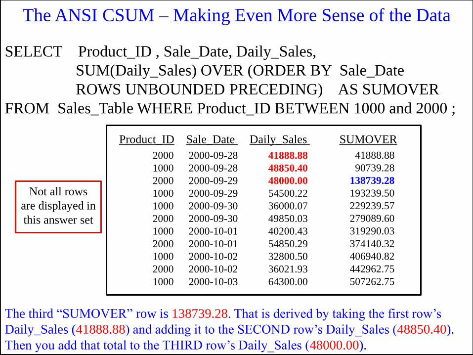
The third “SUMOVER” row is 138739.28. That is derived by taking the first row‟s
Daily_Sales (41888.88) and adding it to the SECOND row‟s Daily_Sales (48850.40).
Then you add that total to the THIRD row‟s Daily_Sales (48000.00).
The ANSI CSUM – Making Even More Sense of the Data
Not all rows
are displayed in
this answer set
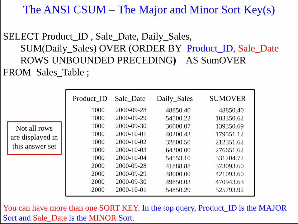
SELECT Product_ID , Sale_Date, Daily_Sales,
SUM(Daily_Sales) OVER (ORDER BY Product_ID, Sale_Date
ROWS UNBOUNDED PRECEDING) AS SumOVER
FROM Sales_Table ;
Product_ID Sale_Date Daily_Sales SUMOVER
You can have more than one SORT KEY. In the top query, Product_ID is the MAJOR
Sort and Sale_Date is the MINOR Sort.
1000
1000
1000
1000
1000
1000
1000
2000
2000
2000
2000
2000-09-28
2000-09-29
2000-09-30
2000-10-01
2000-10-02
2000-10-03
2000-10-04
2000-09-28
2000-09-29
2000-09-30
2000-10-01
48850.40
54500.22
36000.07
40200.43
32800.50
64300.00
54553.10
41888.88
48000.00
49850.03
54850.29
48850.40
103350.62
139350.69
179551.12
212351.62
276651.62
331204.72
373093.60
421093.60
470943.63
525793.92
The ANSI CSUM – The Major and Minor Sort Key(s)
Not all rows
are displayed in
this answer set
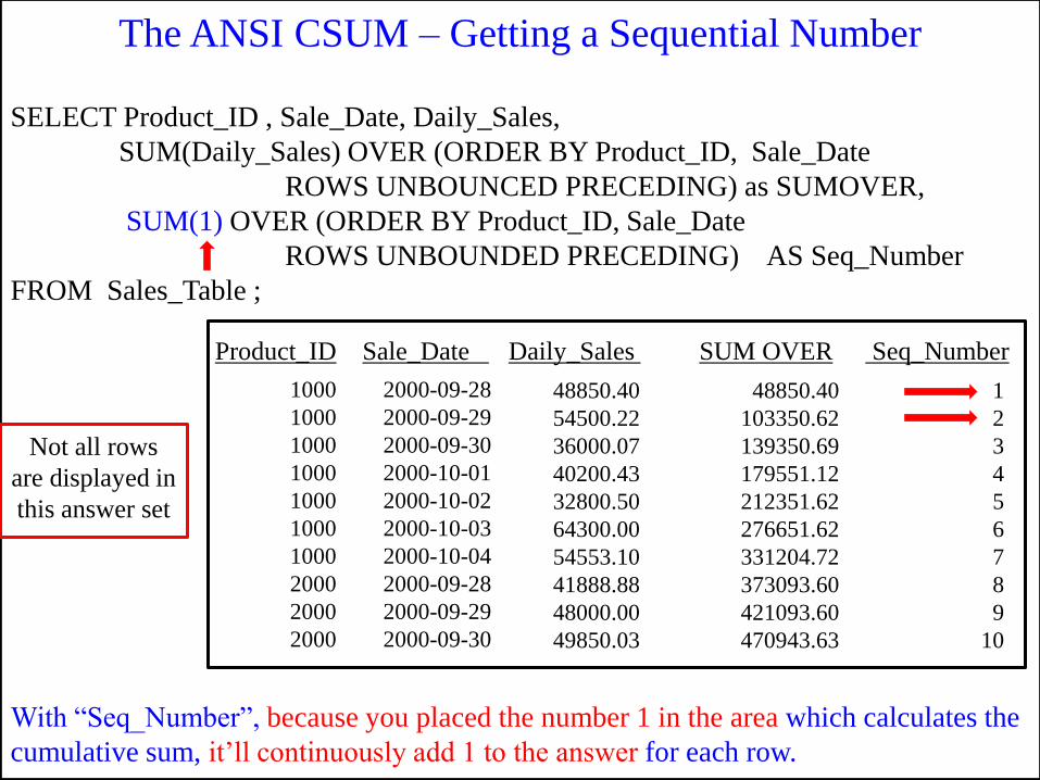
SELECT Product_ID , Sale_Date, Daily_Sales,
SUM(Daily_Sales) OVER (ORDER BY Product_ID, Sale_Date
ROWS UNBOUNCED PRECEDING) as SUMOVER,
SUM(1) OVER (ORDER BY Product_ID, Sale_Date
ROWS UNBOUNDED PRECEDING) AS Seq_Number
FROM Sales_Table ;
Product_ID Sale_Date Daily_Sales SUM OVER Seq_Number
With “Seq_Number”, because you placed the number 1 in the area which calculates the
cumulative sum, it‟ll continuously add 1 to the answer for each row.
1000
1000
1000
1000
1000
1000
1000
2000
2000
2000
2000-09-28
2000-09-29
2000-09-30
2000-10-01
2000-10-02
2000-10-03
2000-10-04
2000-09-28
2000-09-29
2000-09-30
48850.40
54500.22
36000.07
40200.43
32800.50
64300.00
54553.10
41888.88
48000.00
49850.03
48850.40
103350.62
139350.69
179551.12
212351.62
276651.62
331204.72
373093.60
421093.60
470943.63
1
2
3
4
5
6
7
8
9
10
The ANSI CSUM – Getting a Sequential Number
Not all rows
are displayed in
this answer set
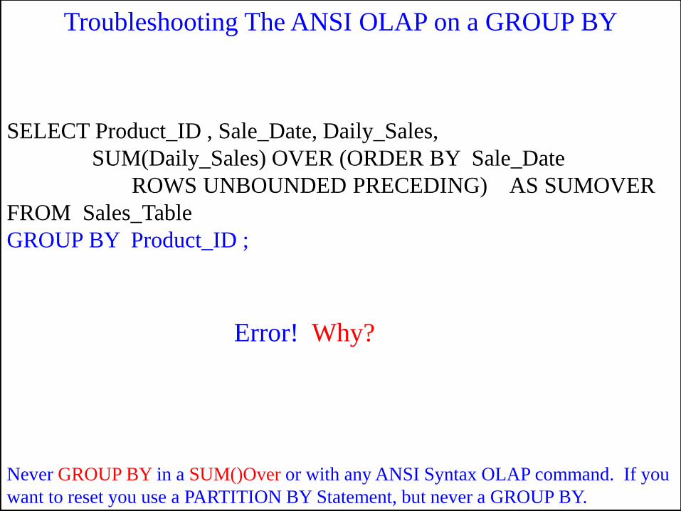
SELECT Product_ID , Sale_Date, Daily_Sales,
SUM(Daily_Sales) OVER (ORDER BY Sale_Date
ROWS UNBOUNDED PRECEDING) AS SUMOVER
FROM Sales_Table
GROUP BY Product_ID ;
Never GROUP BY in a SUM()Over or with any ANSI Syntax OLAP command. If you
want to reset you use a PARTITION BY Statement, but never a GROUP BY.
Error! Why?
Troubleshooting The ANSI OLAP on a GROUP BY
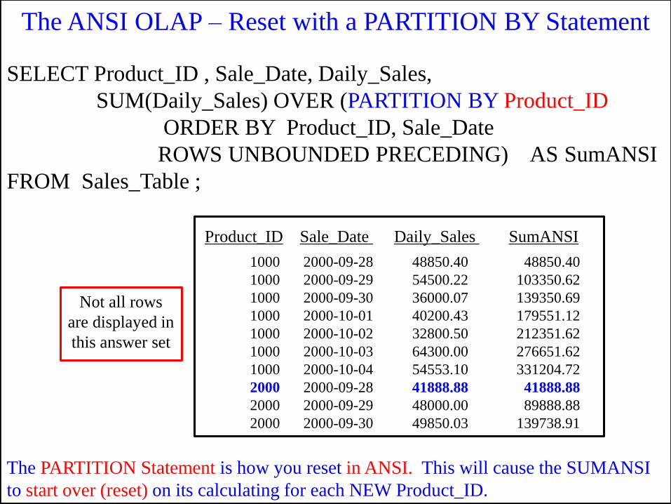
SELECT Product_ID , Sale_Date, Daily_Sales,
SUM(Daily_Sales) OVER (PARTITION BY Product_ID
ORDER BY Product_ID, Sale_Date
ROWS UNBOUNDED PRECEDING) AS SumANSI
FROM Sales_Table ;
Product_ID Sale_Date Daily_Sales SumANSI
The PARTITION Statement is how you reset in ANSI. This will cause the SUMANSI
to start over (reset) on its calculating for each NEW Product_ID.
1000
1000
1000
1000
1000
1000
1000
2000
2000
2000
2000-09-28
2000-09-29
2000-09-30
2000-10-01
2000-10-02
2000-10-03
2000-10-04
2000-09-28
2000-09-29
2000-09-30
48850.40
54500.22
36000.07
40200.43
32800.50
64300.00
54553.10
41888.88
48000.00
49850.03
48850.40
103350.62
139350.69
179551.12
212351.62
276651.62
331204.72
41888.88
89888.88
139738.91
The ANSI OLAP – Reset with a PARTITION BY Statement
Not all rows
are displayed in
this answer set
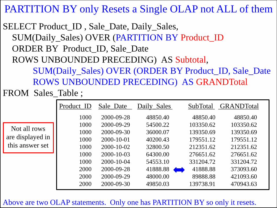
SELECT Product_ID , Sale_Date, Daily_Sales,
SUM(Daily_Sales) OVER (PARTITION BY Product_ID
ORDER BY Product_ID, Sale_Date
ROWS UNBOUNDED PRECEDING) AS Subtotal,
SUM(Daily_Sales) OVER (ORDER BY Product_ID, Sale_Date
ROWS UNBOUNDED PRECEDING) AS GRANDTotal
FROM Sales_Table ;
Product_ID Sale_Date Daily_Sales SubTotal GRANDTotal
1000
1000
1000
1000
1000
1000
1000
2000
2000
2000
2000-09-28
2000-09-29
2000-09-30
2000-10-01
2000-10-02
2000-10-03
2000-10-04
2000-09-28
2000-09-29
2000-09-30
48850.40
54500.22
36000.07
40200.43
32800.50
64300.00
54553.10
41888.88
48000.00
49850.03
48850.40
103350.62
139350.69
179551.12
212351.62
276651.62
331204.72
41888.88
89888.88
139738.91
48850.40
103350.62
139350.69
179551.12
212351.62
276651.62
331204.72
373093.60
421093.60
470943.63
PARTITION BY only Resets a Single OLAP not ALL of them
Above are two OLAP statements. Only one has PARTITION BY so only it resets.
Not all rows
are displayed in
this answer set
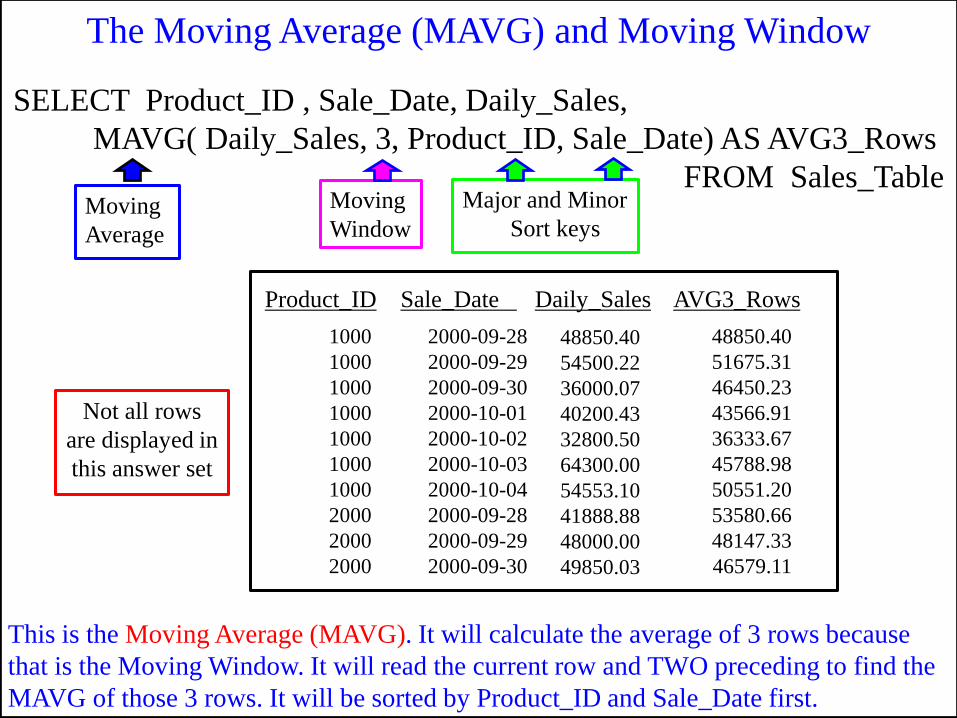
SELECT Product_ID , Sale_Date, Daily_Sales,
MAVG( Daily_Sales, 3, Product_ID, Sale_Date) AS AVG3_Rows
FROM Sales_Table
Product_ID Sale_Date Daily_Sales AVG3_Rows
This is the Moving Average (MAVG). It will calculate the average of 3 rows because
that is the Moving Window. It will read the current row and TWO preceding to find the
MAVG of those 3 rows. It will be sorted by Product_ID and Sale_Date first.
1000
1000
1000
1000
1000
1000
1000
2000
2000
2000
2000-09-28
2000-09-29
2000-09-30
2000-10-01
2000-10-02
2000-10-03
2000-10-04
2000-09-28
2000-09-29
2000-09-30
48850.40
54500.22
36000.07
40200.43
32800.50
64300.00
54553.10
41888.88
48000.00
49850.03
48850.40
51675.31
46450.23
43566.91
36333.67
45788.98
50551.20
53580.66
48147.33
46579.11
Moving
Average
Moving
Window
Major and Minor
Sort keys
The Moving Average (MAVG) and Moving Window
Not all rows
are displayed in
this answer set
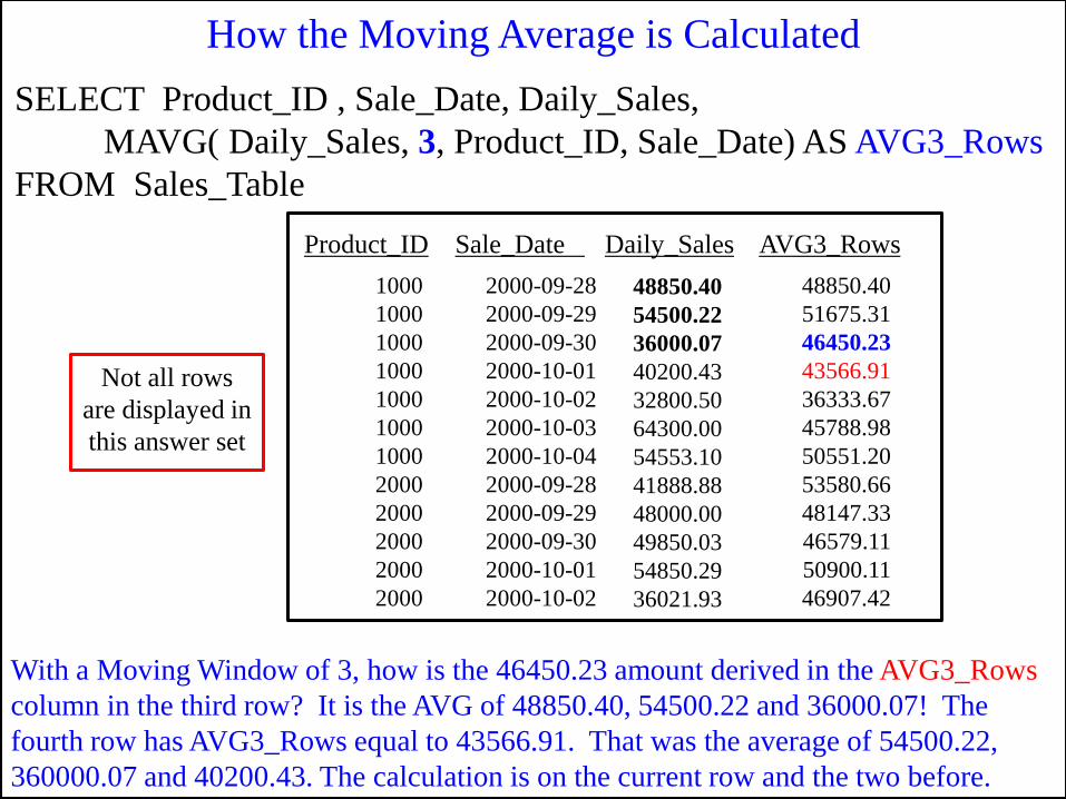
With a Moving Window of 3, how is the 46450.23 amount derived in the AVG3_Rows
column in the third row? It is the AVG of 48850.40, 54500.22 and 36000.07! The
fourth row has AVG3_Rows equal to 43566.91. That was the average of 54500.22,
360000.07 and 40200.43. The calculation is on the current row and the two before.
SELECT Product_ID , Sale_Date, Daily_Sales,
MAVG( Daily_Sales, 3, Product_ID, Sale_Date) AS AVG3_Rows
FROM Sales_Table
Product_ID Sale_Date Daily_Sales AVG3_Rows
1000
1000
1000
1000
1000
1000
1000
2000
2000
2000
2000
2000
2000-09-28
2000-09-29
2000-09-30
2000-10-01
2000-10-02
2000-10-03
2000-10-04
2000-09-28
2000-09-29
2000-09-30
2000-10-01
2000-10-02
48850.40
54500.22
36000.07
40200.43
32800.50
64300.00
54553.10
41888.88
48000.00
49850.03
54850.29
36021.93
48850.40
51675.31
46450.23
43566.91
36333.67
45788.98
50551.20
53580.66
48147.33
46579.11
50900.11
46907.42
How the Moving Average is Calculated
Not all rows
are displayed in
this answer set
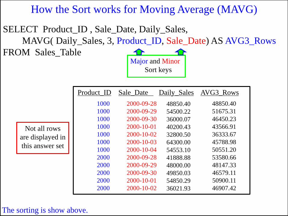
SELECT Product_ID , Sale_Date, Daily_Sales,
MAVG( Daily_Sales, 3, Product_ID, Sale_Date) AS AVG3_Rows
FROM Sales_Table
Product_ID Sale_Date Daily_Sales AVG3_Rows
1000
1000
1000
1000
1000
1000
1000
2000
2000
2000
2000
2000
2000-09-28
2000-09-29
2000-09-30
2000-10-01
2000-10-02
2000-10-03
2000-10-04
2000-09-28
2000-09-29
2000-09-30
2000-10-01
2000-10-02
48850.40
54500.22
36000.07
40200.43
32800.50
64300.00
54553.10
41888.88
48000.00
49850.03
54850.29
36021.93
48850.40
51675.31
46450.23
43566.91
36333.67
45788.98
50551.20
53580.66
48147.33
46579.11
50900.11
46907.42
Major and Minor
Sort keys
How the Sort works for Moving Average (MAVG)
The sorting is show above.
Not all rows
are displayed in
this answer set
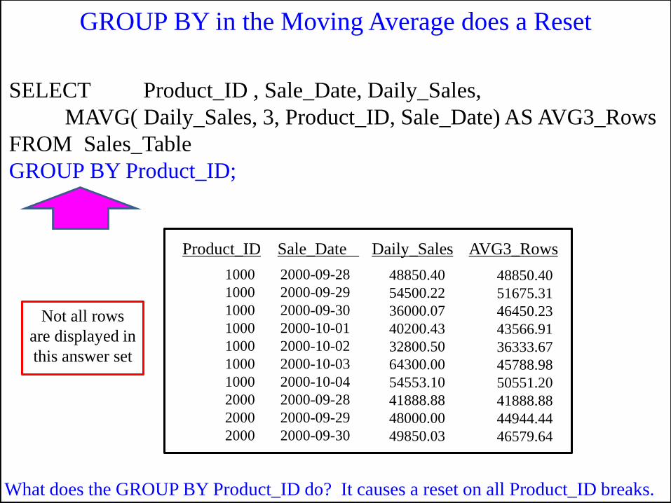
SELECT Product_ID , Sale_Date, Daily_Sales,
MAVG( Daily_Sales, 3, Product_ID, Sale_Date) AS AVG3_Rows
FROM Sales_Table
GROUP BY Product_ID;
What does the GROUP BY Product_ID do? It causes a reset on all Product_ID breaks.
Product_ID Sale_Date Daily_Sales AVG3_Rows
1000
1000
1000
1000
1000
1000
1000
2000
2000
2000
2000-09-28
2000-09-29
2000-09-30
2000-10-01
2000-10-02
2000-10-03
2000-10-04
2000-09-28
2000-09-29
2000-09-30
48850.40
54500.22
36000.07
40200.43
32800.50
64300.00
54553.10
41888.88
48000.00
49850.03
48850.40
51675.31
46450.23
43566.91
36333.67
45788.98
50551.20
41888.88
44944.44
46579.64
GROUP BY in the Moving Average does a Reset
Not all rows
are displayed in
this answer set
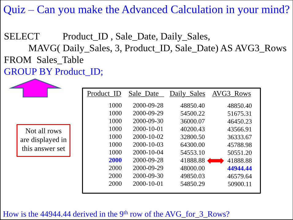
How is the 44944.44 derived in the 9th row of the AVG_for_3_Rows?
SELECT Product_ID , Sale_Date, Daily_Sales,
MAVG( Daily_Sales, 3, Product_ID, Sale_Date) AS AVG3_Rows
FROM Sales_Table
GROUP BY Product_ID;
Product_ID Sale_Date Daily_Sales AVG3_Rows
1000
1000
1000
1000
1000
1000
1000
2000
2000
2000
2000
2000-09-28
2000-09-29
2000-09-30
2000-10-01
2000-10-02
2000-10-03
2000-10-04
2000-09-28
2000-09-29
2000-09-30
2000-10-01
48850.40
54500.22
36000.07
40200.43
32800.50
64300.00
54553.10
41888.88
48000.00
49850.03
54850.29
48850.40
51675.31
46450.23
43566.91
36333.67
45788.98
50551.20
41888.88
44944.44
46579.64
50900.11
Quiz – Can you make the Advanced Calculation in your mind?
Not all rows
are displayed in
this answer set
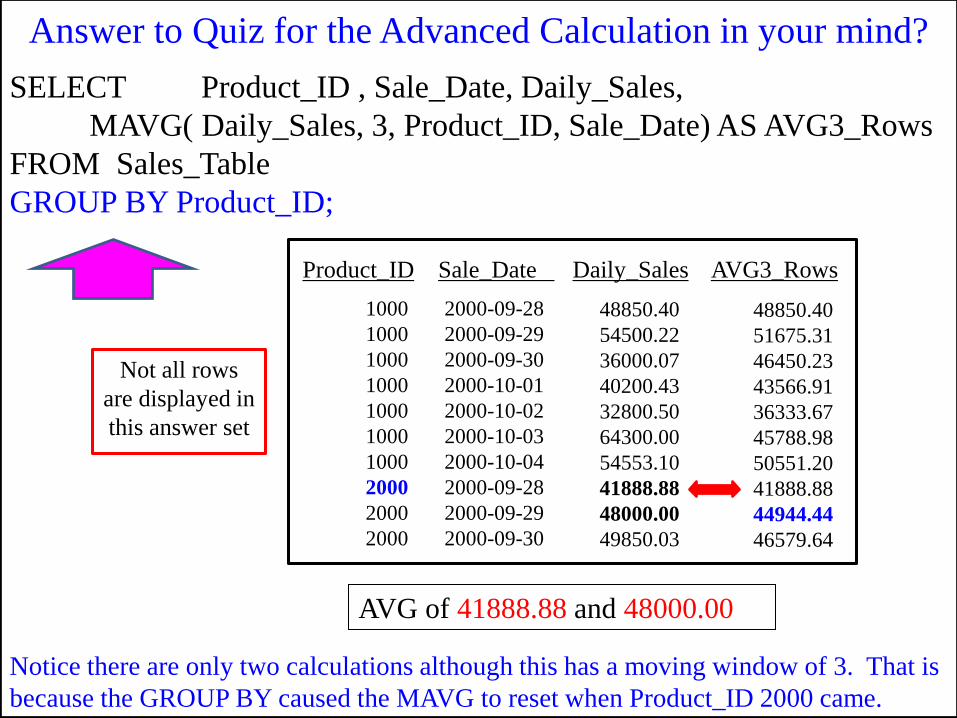
AVG of 41888.88 and 48000.00
SELECT Product_ID , Sale_Date, Daily_Sales,
MAVG( Daily_Sales, 3, Product_ID, Sale_Date) AS AVG3_Rows
FROM Sales_Table
GROUP BY Product_ID;
Product_ID Sale_Date Daily_Sales AVG3_Rows
1000
1000
1000
1000
1000
1000
1000
2000
2000
2000
2000-09-28
2000-09-29
2000-09-30
2000-10-01
2000-10-02
2000-10-03
2000-10-04
2000-09-28
2000-09-29
2000-09-30
48850.40
54500.22
36000.07
40200.43
32800.50
64300.00
54553.10
41888.88
48000.00
49850.03
48850.40
51675.31
46450.23
43566.91
36333.67
45788.98
50551.20
41888.88
44944.44
46579.64
Answer to Quiz for the Advanced Calculation in your mind?
Notice there are only two calculations although this has a moving window of 3. That is
because the GROUP BY caused the MAVG to reset when Product_ID 2000 came.
Not all rows
are displayed in
this answer set
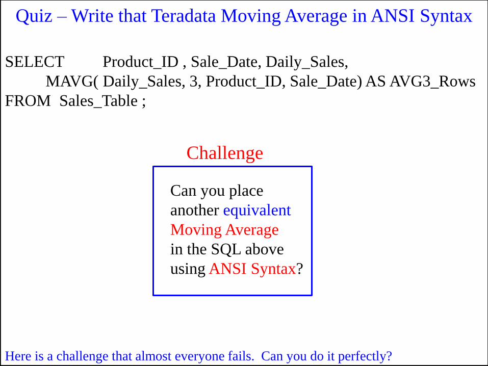
SELECT Product_ID , Sale_Date, Daily_Sales,
MAVG( Daily_Sales, 3, Product_ID, Sale_Date) AS AVG3_Rows
FROM Sales_Table ;
Challenge
Can you place
another equivalent
Moving Average
in the SQL above
using ANSI Syntax?
Quiz – Write that Teradata Moving Average in ANSI Syntax
Here is a challenge that almost everyone fails. Can you do it perfectly?
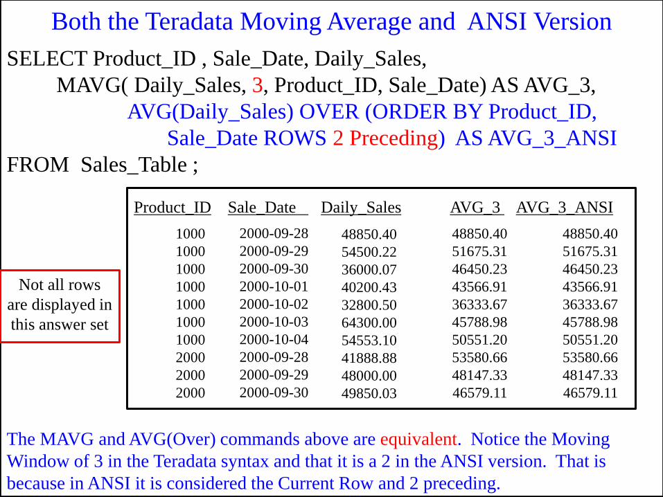
SELECT Product_ID , Sale_Date, Daily_Sales,
MAVG( Daily_Sales, 3, Product_ID, Sale_Date) AS AVG_3,
AVG(Daily_Sales) OVER (ORDER BY Product_ID,
Sale_Date ROWS 2 Preceding) AS AVG_3_ANSI
FROM Sales_Table ;
Product_ID Sale_Date Daily_Sales AVG_3 AVG_3_ANSI
The MAVG and AVG(Over) commands above are equivalent. Notice the Moving
Window of 3 in the Teradata syntax and that it is a 2 in the ANSI version. That is
because in ANSI it is considered the Current Row and 2 preceding.
1000
1000
1000
1000
1000
1000
1000
2000
2000
2000
2000-09-28
2000-09-29
2000-09-30
2000-10-01
2000-10-02
2000-10-03
2000-10-04
2000-09-28
2000-09-29
2000-09-30
48850.40
54500.22
36000.07
40200.43
32800.50
64300.00
54553.10
41888.88
48000.00
49850.03
48850.40
51675.31
46450.23
43566.91
36333.67
45788.98
50551.20
53580.66
48147.33
46579.11
48850.40
51675.31
46450.23
43566.91
36333.67
45788.98
50551.20
53580.66
48147.33
46579.11
Both the Teradata Moving Average and ANSI Version
Not all rows
are displayed in
this answer set
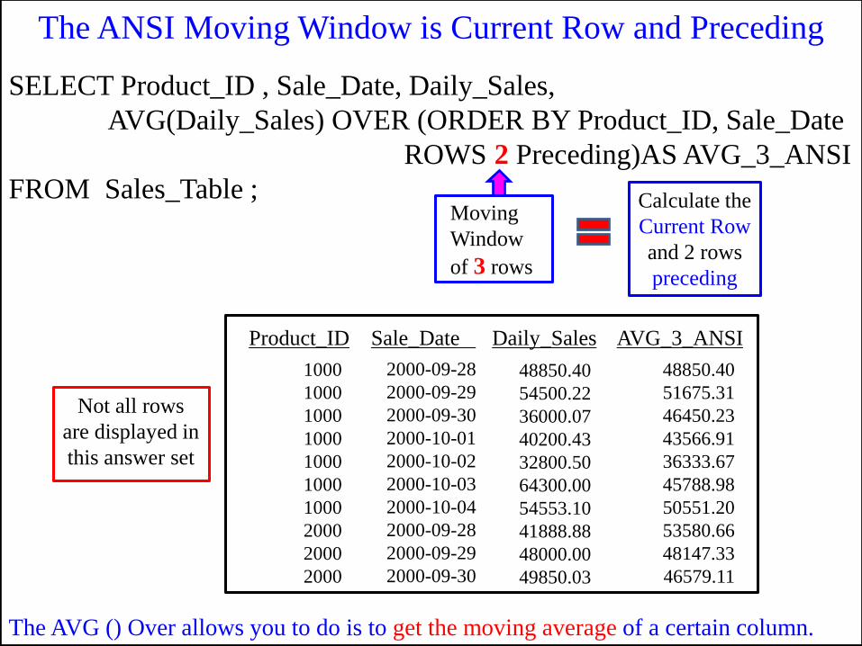
SELECT Product_ID , Sale_Date, Daily_Sales,
AVG(Daily_Sales) OVER (ORDER BY Product_ID, Sale_Date
ROWS 2 Preceding)AS AVG_3_ANSI
FROM Sales_Table ;
Product_ID Sale_Date Daily_Sales AVG_3_ANSI
The AVG () Over allows you to do is to get the moving average of a certain column.
1000
1000
1000
1000
1000
1000
1000
2000
2000
2000
2000-09-28
2000-09-29
2000-09-30
2000-10-01
2000-10-02
2000-10-03
2000-10-04
2000-09-28
2000-09-29
2000-09-30
48850.40
54500.22
36000.07
40200.43
32800.50
64300.00
54553.10
41888.88
48000.00
49850.03
48850.40
51675.31
46450.23
43566.91
36333.67
45788.98
50551.20
53580.66
48147.33
46579.11
Moving
Window
of 3 rows
Calculate the
Current Row
and 2 rows
preceding
The ANSI Moving Window is Current Row and Preceding
Not all rows
are displayed in
this answer set
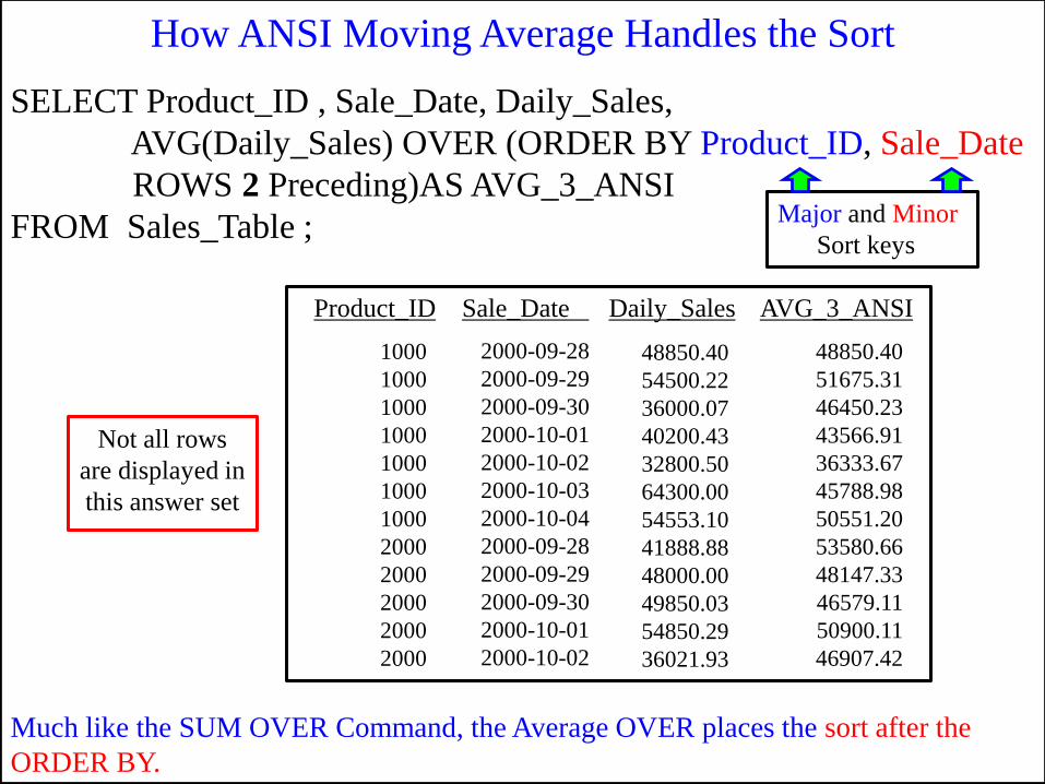
Much like the SUM OVER Command, the Average OVER places the sort after the
ORDER BY.
SELECT Product_ID , Sale_Date, Daily_Sales,
AVG(Daily_Sales) OVER (ORDER BY Product_ID, Sale_Date
ROWS 2 Preceding)AS AVG_3_ANSI
FROM Sales_Table ;
Product_ID Sale_Date Daily_Sales AVG_3_ANSI
1000
1000
1000
1000
1000
1000
1000
2000
2000
2000
2000
2000
2000-09-28
2000-09-29
2000-09-30
2000-10-01
2000-10-02
2000-10-03
2000-10-04
2000-09-28
2000-09-29
2000-09-30
2000-10-01
2000-10-02
48850.40
54500.22
36000.07
40200.43
32800.50
64300.00
54553.10
41888.88
48000.00
49850.03
54850.29
36021.93
48850.40
51675.31
46450.23
43566.91
36333.67
45788.98
50551.20
53580.66
48147.33
46579.11
50900.11
46907.42
Major and Minor
Sort keys
How ANSI Moving Average Handles the Sort
Not all rows
are displayed in
this answer set
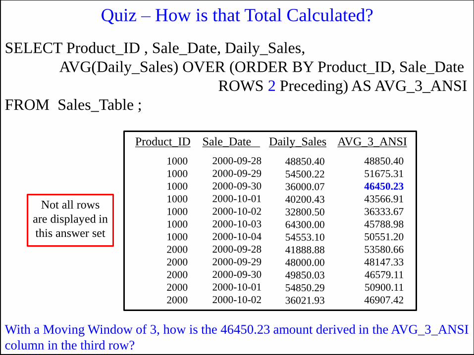
With a Moving Window of 3, how is the 46450.23 amount derived in the AVG_3_ANSI
column in the third row?
Product_ID Sale_Date Daily_Sales AVG_3_ANSI
1000
1000
1000
1000
1000
1000
1000
2000
2000
2000
2000
2000
2000-09-28
2000-09-29
2000-09-30
2000-10-01
2000-10-02
2000-10-03
2000-10-04
2000-09-28
2000-09-29
2000-09-30
2000-10-01
2000-10-02
48850.40
54500.22
36000.07
40200.43
32800.50
64300.00
54553.10
41888.88
48000.00
49850.03
54850.29
36021.93
48850.40
51675.31
46450.23
43566.91
36333.67
45788.98
50551.20
53580.66
48147.33
46579.11
50900.11
46907.42
SELECT Product_ID , Sale_Date, Daily_Sales,
AVG(Daily_Sales) OVER (ORDER BY Product_ID, Sale_Date
ROWS 2 Preceding) AS AVG_3_ANSI
FROM Sales_Table ;
Quiz – How is that Total Calculated?
Not all rows
are displayed in
this answer set
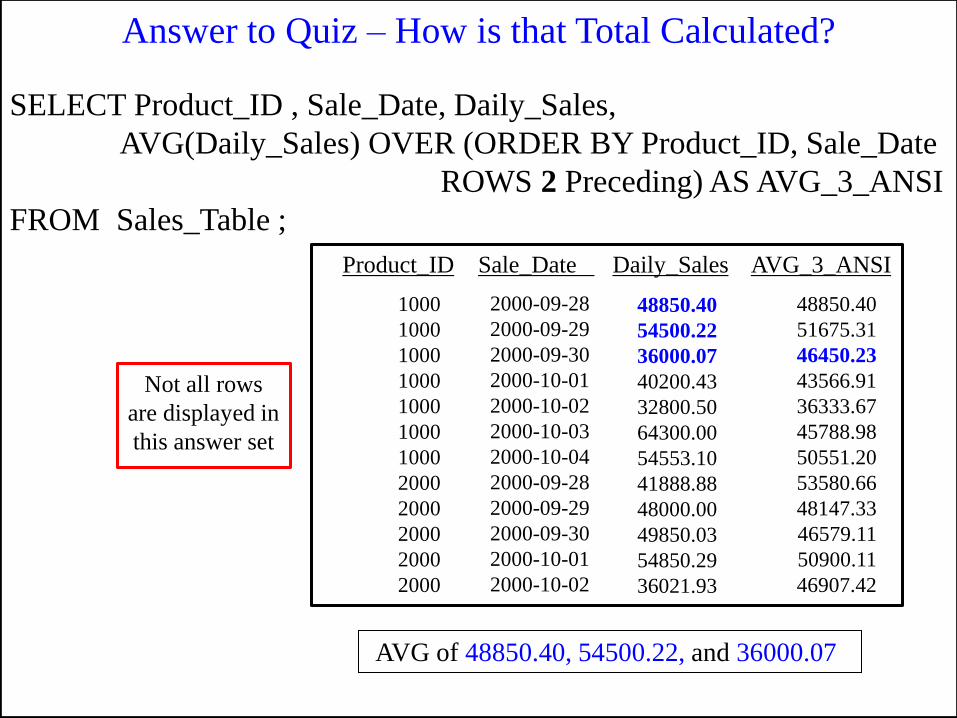
AVG of 48850.40, 54500.22, and 36000.07
Product_ID Sale_Date Daily_Sales AVG_3_ANSI
1000
1000
1000
1000
1000
1000
1000
2000
2000
2000
2000
2000
2000-09-28
2000-09-29
2000-09-30
2000-10-01
2000-10-02
2000-10-03
2000-10-04
2000-09-28
2000-09-29
2000-09-30
2000-10-01
2000-10-02
48850.40
54500.22
36000.07
40200.43
32800.50
64300.00
54553.10
41888.88
48000.00
49850.03
54850.29
36021.93
48850.40
51675.31
46450.23
43566.91
36333.67
45788.98
50551.20
53580.66
48147.33
46579.11
50900.11
46907.42
SELECT Product_ID , Sale_Date, Daily_Sales,
AVG(Daily_Sales) OVER (ORDER BY Product_ID, Sale_Date
ROWS 2 Preceding) AS AVG_3_ANSI
FROM Sales_Table ;
Answer to Quiz – How is that Total Calculated?
Not all rows
are displayed in
this answer set
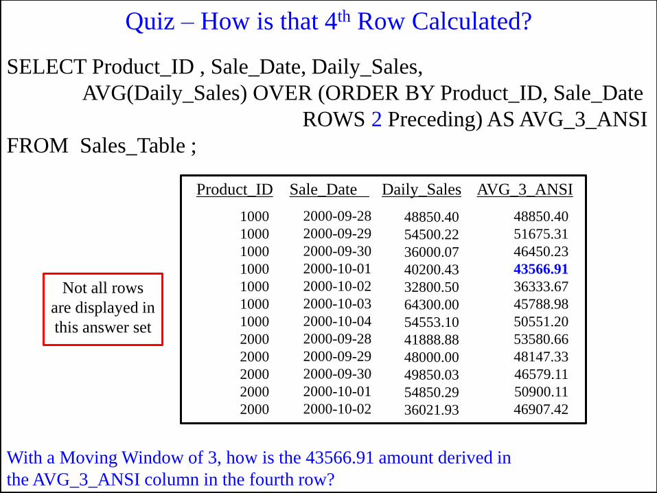
Product_ID Sale_Date Daily_Sales AVG_3_ANSI
1000
1000
1000
1000
1000
1000
1000
2000
2000
2000
2000
2000
2000-09-28
2000-09-29
2000-09-30
2000-10-01
2000-10-02
2000-10-03
2000-10-04
2000-09-28
2000-09-29
2000-09-30
2000-10-01
2000-10-02
48850.40
54500.22
36000.07
40200.43
32800.50
64300.00
54553.10
41888.88
48000.00
49850.03
54850.29
36021.93
48850.40
51675.31
46450.23
43566.91
36333.67
45788.98
50551.20
53580.66
48147.33
46579.11
50900.11
46907.42
SELECT Product_ID , Sale_Date, Daily_Sales,
AVG(Daily_Sales) OVER (ORDER BY Product_ID, Sale_Date
ROWS 2 Preceding) AS AVG_3_ANSI
FROM Sales_Table ;
With a Moving Window of 3, how is the 43566.91 amount derived in
the AVG_3_ANSI column in the fourth row?
Quiz – How is that 4th Row Calculated?
Not all rows
are displayed in
this answer set
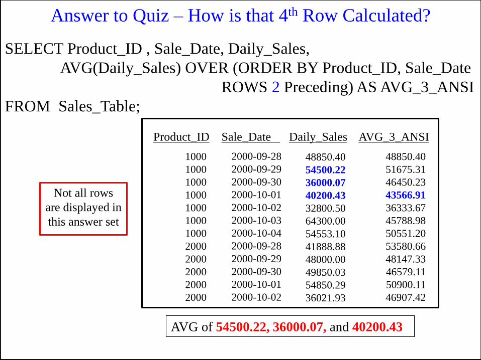
Product_ID Sale_Date Daily_Sales AVG_3_ANSI
1000
1000
1000
1000
1000
1000
1000
2000
2000
2000
2000
2000
2000-09-28
2000-09-29
2000-09-30
2000-10-01
2000-10-02
2000-10-03
2000-10-04
2000-09-28
2000-09-29
2000-09-30
2000-10-01
2000-10-02
48850.40
54500.22
36000.07
40200.43
32800.50
64300.00
54553.10
41888.88
48000.00
49850.03
54850.29
36021.93
48850.40
51675.31
46450.23
43566.91
36333.67
45788.98
50551.20
53580.66
48147.33
46579.11
50900.11
46907.42
SELECT Product_ID , Sale_Date, Daily_Sales,
AVG(Daily_Sales) OVER (ORDER BY Product_ID, Sale_Date
ROWS 2 Preceding) AS AVG_3_ANSI
FROM Sales_Table;
AVG of 54500.22, 36000.07, and 40200.43
Answer to Quiz – How is that 4th Row Calculated?
Not all rows
are displayed in
this answer set
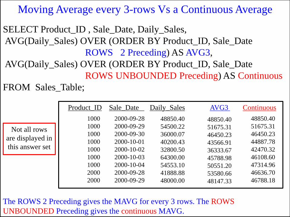
SELECT Product_ID , Sale_Date, Daily_Sales,
AVG(Daily_Sales) OVER (ORDER BY Product_ID, Sale_Date
ROWS 2 Preceding) AS AVG3,
AVG(Daily_Sales) OVER (ORDER BY Product_ID, Sale_Date
ROWS UNBOUNDED Preceding) AS Continuous
FROM Sales_Table;
Product_ID Sale_Date Daily_Sales AVG3 Continuous
The ROWS 2 Preceding gives the MAVG for every 3 rows. The ROWS
UNBOUNDED Preceding gives the continuous MAVG.
1000
1000
1000
1000
1000
1000
1000
2000
2000
2000-09-28
2000-09-29
2000-09-30
2000-10-01
2000-10-02
2000-10-03
2000-10-04
2000-09-28
2000-09-29
48850.40
54500.22
36000.07
40200.43
32800.50
64300.00
54553.10
41888.88
48000.00
48850.40
51675.31
46450.23
43566.91
36333.67
45788.98
50551.20
53580.66
48147.33
48850.40
51675.31
46450.23
44887.78
42470.32
46108.60
47314.96
46636.70
46788.18
Moving Average every 3-rows Vs a Continuous Average
Not all rows
are displayed in
this answer set
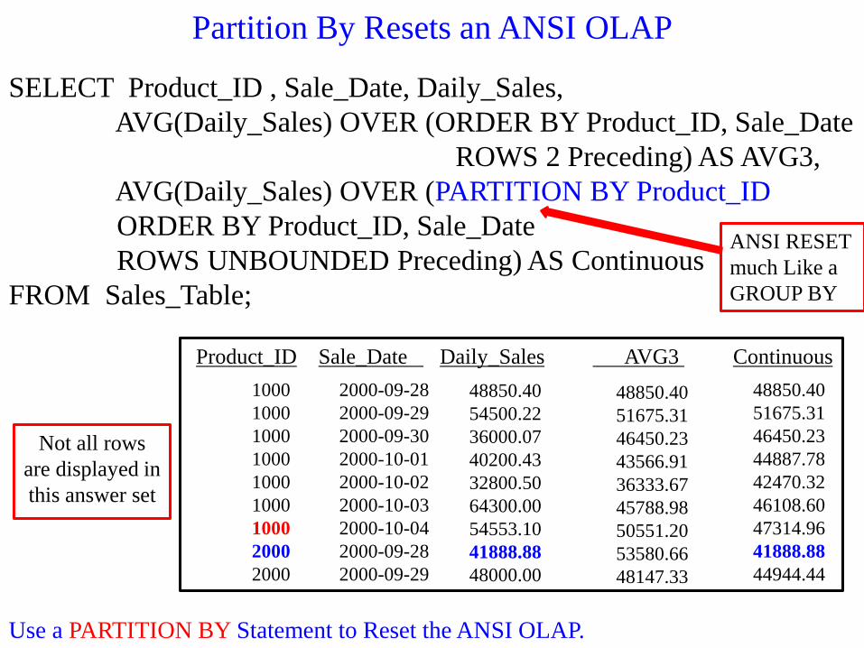
SELECT Product_ID , Sale_Date, Daily_Sales,
AVG(Daily_Sales) OVER (ORDER BY Product_ID, Sale_Date
ROWS 2 Preceding) AS AVG3,
AVG(Daily_Sales) OVER (PARTITION BY Product_ID
ORDER BY Product_ID, Sale_Date
ROWS UNBOUNDED Preceding) AS Continuous
FROM Sales_Table;
Product_ID Sale_Date Daily_Sales AVG3 Continuous
Use a PARTITION BY Statement to Reset the ANSI OLAP.
1000
1000
1000
1000
1000
1000
1000
2000
2000
2000-09-28
2000-09-29
2000-09-30
2000-10-01
2000-10-02
2000-10-03
2000-10-04
2000-09-28
2000-09-29
48850.40
54500.22
36000.07
40200.43
32800.50
64300.00
54553.10
41888.88
48000.00
48850.40
51675.31
46450.23
43566.91
36333.67
45788.98
50551.20
53580.66
48147.33
48850.40
51675.31
46450.23
44887.78
42470.32
46108.60
47314.96
41888.88
44944.44
ANSI RESET
much Like a
GROUP BY
Partition By Resets an ANSI OLAP
Not all rows
are displayed in
this answer set
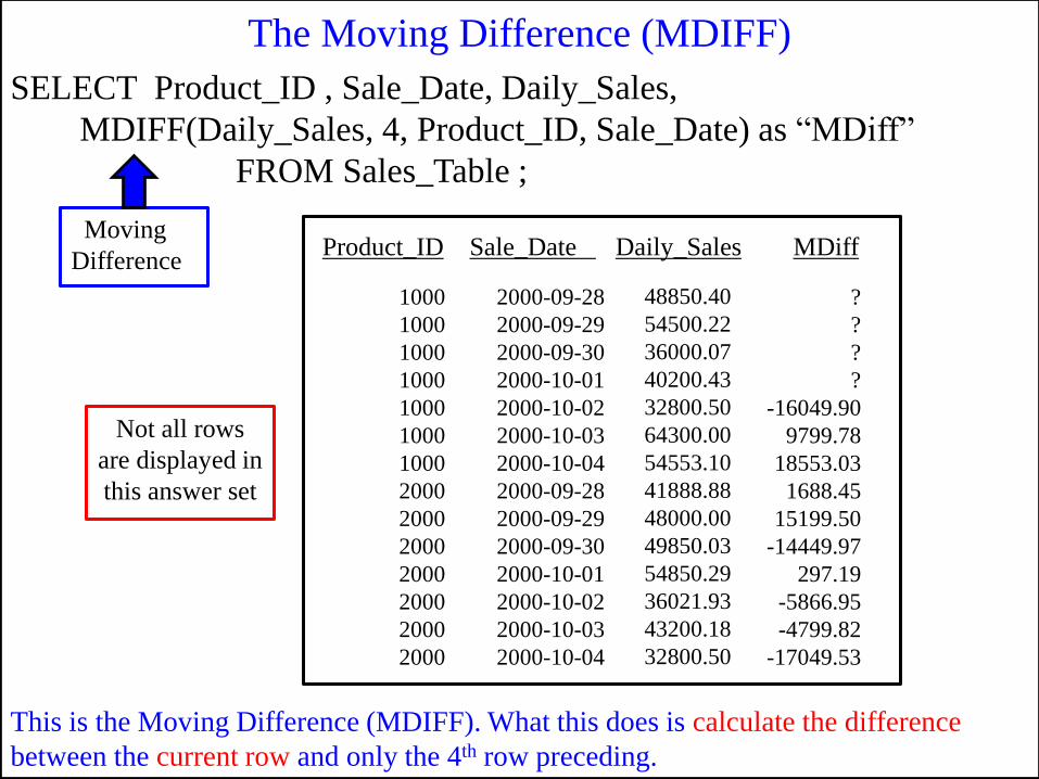
SELECT Product_ID , Sale_Date, Daily_Sales,
MDIFF(Daily_Sales, 4, Product_ID, Sale_Date) as “MDiff”
FROM Sales_Table ;
Product_ID Sale_Date Daily_Sales MDiff
This is the Moving Difference (MDIFF). What this does is calculate the difference
between the current row and only the 4th row preceding.
1000
1000
1000
1000
1000
1000
1000
2000
2000
2000
2000
2000
2000
2000
2000-09-28
2000-09-29
2000-09-30
2000-10-01
2000-10-02
2000-10-03
2000-10-04
2000-09-28
2000-09-29
2000-09-30
2000-10-01
2000-10-02
2000-10-03
2000-10-04
48850.40
54500.22
36000.07
40200.43
32800.50
64300.00
54553.10
41888.88
48000.00
49850.03
54850.29
36021.93
43200.18
32800.50
?
?
?
?
-16049.90
9799.78
18553.03
1688.45
15199.50
-14449.97
297.19
-5866.95
-4799.82
-17049.53
Moving
Difference
The Moving Difference (MDIFF)
Not all rows
are displayed in
this answer set
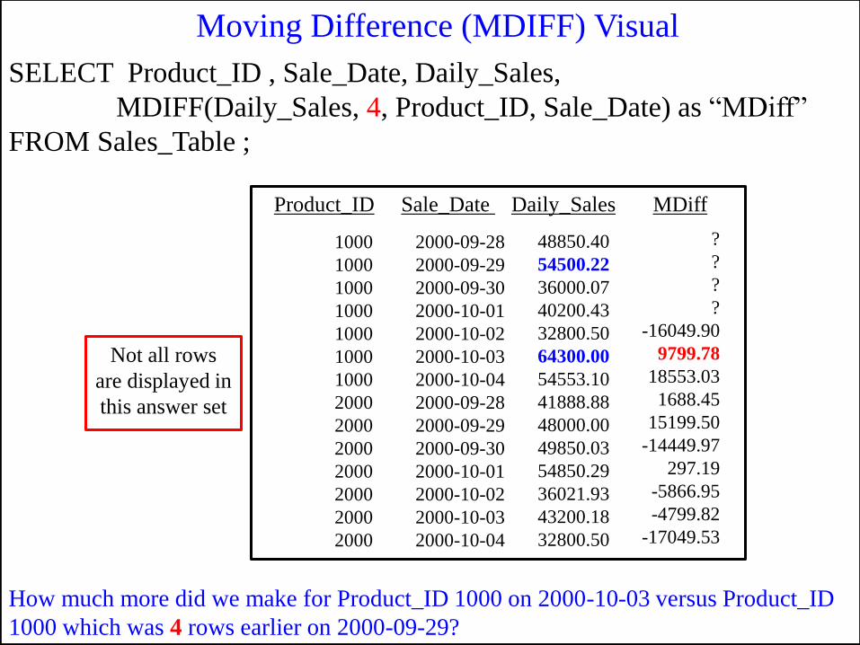
SELECT Product_ID , Sale_Date, Daily_Sales,
MDIFF(Daily_Sales, 4, Product_ID, Sale_Date) as “MDiff”
FROM Sales_Table ;
How much more did we make for Product_ID 1000 on 2000-10-03 versus Product_ID
1000 which was 4 rows earlier on 2000-09-29?
Moving Difference (MDIFF) Visual
Product_ID Sale_Date Daily_Sales MDiff
1000
1000
1000
1000
1000
1000
1000
2000
2000
2000
2000
2000
2000
2000
2000-09-28
2000-09-29
2000-09-30
2000-10-01
2000-10-02
2000-10-03
2000-10-04
2000-09-28
2000-09-29
2000-09-30
2000-10-01
2000-10-02
2000-10-03
2000-10-04
48850.40
54500.22
36000.07
40200.43
32800.50
64300.00
54553.10
41888.88
48000.00
49850.03
54850.29
36021.93
43200.18
32800.50
?
?
?
?
-16049.90
9799.78
18553.03
1688.45
15199.50
-14449.97
297.19
-5866.95
-4799.82
-17049.53
Not all rows
are displayed in
this answer set
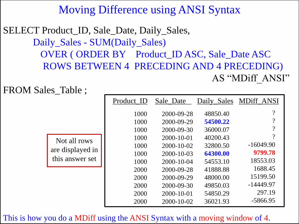
SELECT Product_ID, Sale_Date, Daily_Sales,
Daily_Sales - SUM(Daily_Sales)
OVER ( ORDER BY Product_ID ASC, Sale_Date ASC
ROWS BETWEEN 4 PRECEDING AND 4 PRECEDING)
AS “MDiff_ANSI”
FROM Sales_Table ; Product_ID Sale_Date Daily_Sales MDiff_ANSI
1000
1000
1000
1000
1000
1000
1000
2000
2000
2000
2000
2000
2000-09-28
2000-09-29
2000-09-30
2000-10-01
2000-10-02
2000-10-03
2000-10-04
2000-09-28
2000-09-29
2000-09-30
2000-10-01
2000-10-02
48850.40
54500.22
36000.07
40200.43
32800.50
64300.00
54553.10
41888.88
48000.00
49850.03
54850.29
36021.93
?
?
?
?
-16049.90
9799.78
18553.03
1688.45
15199.50
-14449.97
297.19
-5866.95
This is how you do a MDiff using the ANSI Syntax with a moving window of 4.
Moving Difference using ANSI Syntax
Not all rows
are displayed in
this answer set
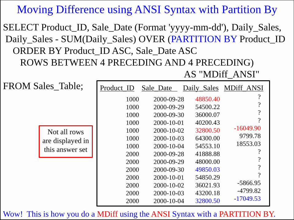
SELECT Product_ID, Sale_Date (Format 'yyyy-mm-dd'), Daily_Sales,
Daily_Sales - SUM(Daily_Sales) OVER (PARTITION BY Product_ID
ORDER BY Product_ID ASC, Sale_Date ASC
ROWS BETWEEN 4 PRECEDING AND 4 PRECEDING)
AS "MDiff_ANSI"
FROM Sales_Table; Product_ID Sale_Date Daily_Sales MDiff_ANSI
1000
1000
1000
1000
1000
1000
1000
2000
2000
2000
2000
2000
2000
2000
2000-09-28
2000-09-29
2000-09-30
2000-10-01
2000-10-02
2000-10-03
2000-10-04
2000-09-28
2000-09-29
2000-09-30
2000-10-01
2000-10-02
2000-10-03
2000-10-04
48850.40
54500.22
36000.07
40200.43
32800.50
64300.00
54553.10
41888.88
48000.00
49850.03
54850.29
36021.93
43200.18
32800.50
?
?
?
?
-16049.90
9799.78
18553.03
?
?
?
?
-5866.95
-4799.82
-17049.53
Wow! This is how you do a MDiff using the ANSI Syntax with a PARTITION BY.
Moving Difference using ANSI Syntax with Partition By
Not all rows
are displayed in
this answer set

SELECT Product_ID , Sale_Date, Daily_Sales,
MDIFF(Daily_Sales, 7, Product_ID, Sale_Date) as Compare2Rows
FROM Sales_Table
GROUP BY Product_ID ; Product_ID Sale_Date Daily_Sales Compare2Rows
Do you notice that column Compare2Rows did not produce any data? That is because
the GROUP BY Reset before it could get 7 records to find the MDIFF.
1000
1000
1000
1000
1000
1000
1000
2000
2000
2000
2000
2000
2000
2000
2000-09-28
2000-09-29
2000-09-30
2000-10-01
2000-10-02
2000-10-03
2000-10-04
2000-09-28
2000-09-29
2000-09-30
2000-10-01
2000-10-02
2000-10-03
2000-10-04
48850.40
54500.22
36000.07
40200.43
32800.50
64300.00
54553.10
41888.88
48000.00
49850.03
54850.29
36021.93
43200.18
32800.50
?
?
?
?
?
?
?
?
?
?
?
?
?
?
Trouble Shooting the Moving Difference (MDIFF)
Not all rows
are displayed in
this answer set
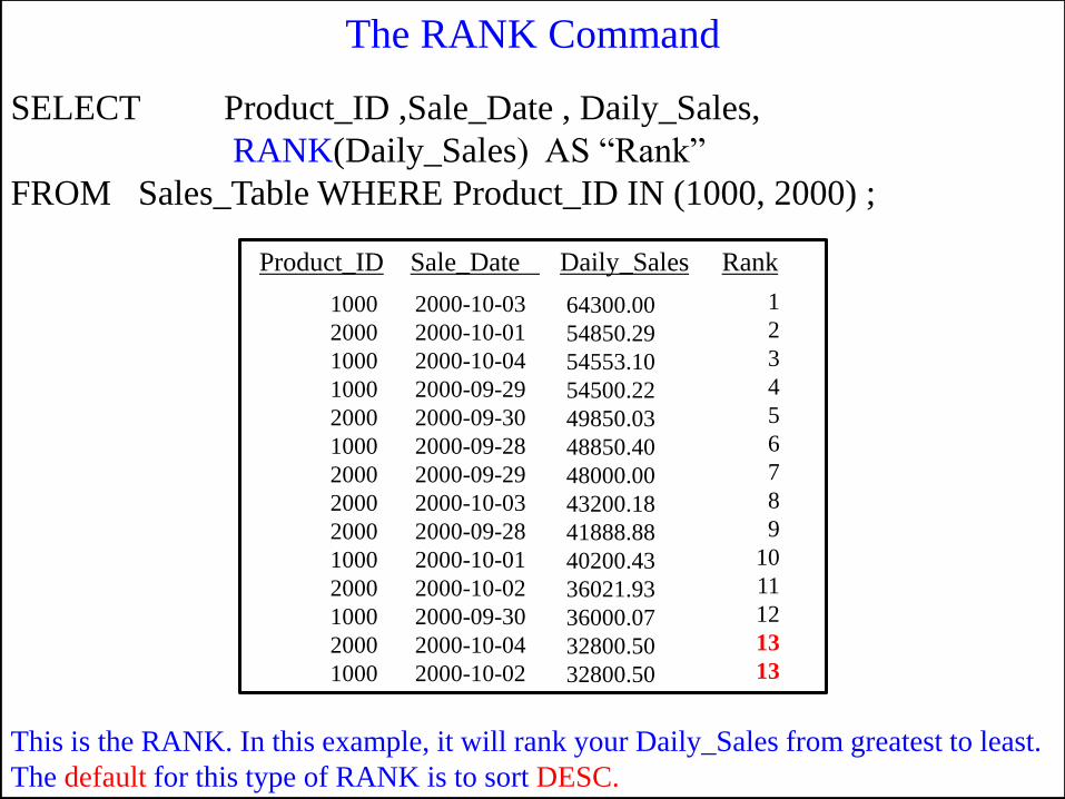
SELECT Product_ID ,Sale_Date , Daily_Sales,
RANK(Daily_Sales) AS “Rank”
FROM Sales_Table WHERE Product_ID IN (1000, 2000) ;
Product_ID Sale_Date Daily_Sales Rank
This is the RANK. In this example, it will rank your Daily_Sales from greatest to least.
The default for this type of RANK is to sort DESC.
1000
2000
1000
1000
2000
1000
2000
2000
2000
1000
2000
1000
2000
1000
2000-10-03
2000-10-01
2000-10-04
2000-09-29
2000-09-30
2000-09-28
2000-09-29
2000-10-03
2000-09-28
2000-10-01
2000-10-02
2000-09-30
2000-10-04
2000-10-02
64300.00
54850.29
54553.10
54500.22
49850.03
48850.40
48000.00
43200.18
41888.88
40200.43
36021.93
36000.07
32800.50
32800.50
1
2
3
4
5
6
7
8
9
10
11
12
13
13
The RANK Command
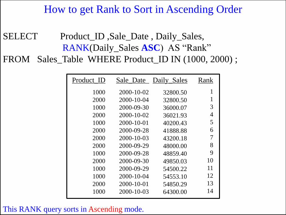
SELECT Product_ID ,Sale_Date , Daily_Sales,
RANK(Daily_Sales ASC) AS “Rank”
FROM Sales_Table WHERE Product_ID IN (1000, 2000) ;
Product_ID Sale_Date Daily_Sales Rank
This RANK query sorts in Ascending mode.
1000
2000
1000
2000
1000
2000
2000
2000
1000
2000
1000
1000
2000
1000
2000-10-02
2000-10-04
2000-09-30
2000-10-02
2000-10-01
2000-09-28
2000-10-03
2000-09-29
2000-09-28
2000-09-30
2000-09-29
2000-10-04
2000-10-01
2000-10-03
32800.50
32800.50
36000.07
36021.93
40200.43
41888.88
43200.18
48000.00
48859.40
49850.03
54500.22
54553.10
54850.29
64300.00
1
1
3
4
5
6
7
8
9
10
11
12
13
14
How to get Rank to Sort in Ascending Order
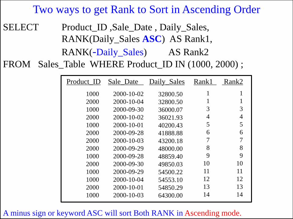
Product_ID Sale_Date Daily_Sales Rank1 Rank2
1000
2000
1000
2000
1000
2000
2000
2000
1000
2000
1000
1000
2000
1000
2000-10-02
2000-10-04
2000-09-30
2000-10-02
2000-10-01
2000-09-28
2000-10-03
2000-09-29
2000-09-28
2000-09-30
2000-09-29
2000-10-04
2000-10-01
2000-10-03
32800.50
32800.50
36000.07
36021.93
40200.43
41888.88
43200.18
48000.00
48859.40
49850.03
54500.22
54553.10
54850.29
64300.00
1
1
3
4
5
6
7
8
9
10
11
12
13
14
SELECT Product_ID ,Sale_Date , Daily_Sales,
RANK(Daily_Sales ASC) AS Rank1,
RANK(-Daily_Sales) AS Rank2
FROM Sales_Table WHERE Product_ID IN (1000, 2000) ;
1
1
3
4
5
6
7
8
9
10
11
12
13
14
A minus sign or keyword ASC will sort Both RANK in Ascending mode.
Two ways to get Rank to Sort in Ascending Order
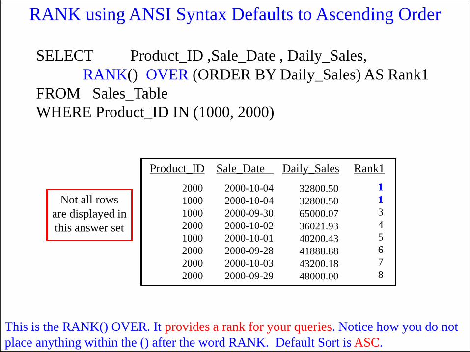
SELECT Product_ID ,Sale_Date , Daily_Sales,
RANK() OVER (ORDER BY Daily_Sales) AS Rank1
FROM Sales_Table
WHERE Product_ID IN (1000, 2000)
This is the RANK() OVER. It provides a rank for your queries. Notice how you do not
place anything within the () after the word RANK. Default Sort is ASC.
RANK using ANSI Syntax Defaults to Ascending Order
Product_ID Sale_Date Daily_Sales Rank1
2000
1000
1000
2000
1000
2000
2000
2000
2000-10-04
2000-10-04
2000-09-30
2000-10-02
2000-10-01
2000-09-28
2000-10-03
2000-09-29
32800.50
32800.50
65000.07
36021.93
40200.43
41888.88
43200.18
48000.00
1
1
3
4
5
6
7
8
Not all rows
are displayed in
this answer set
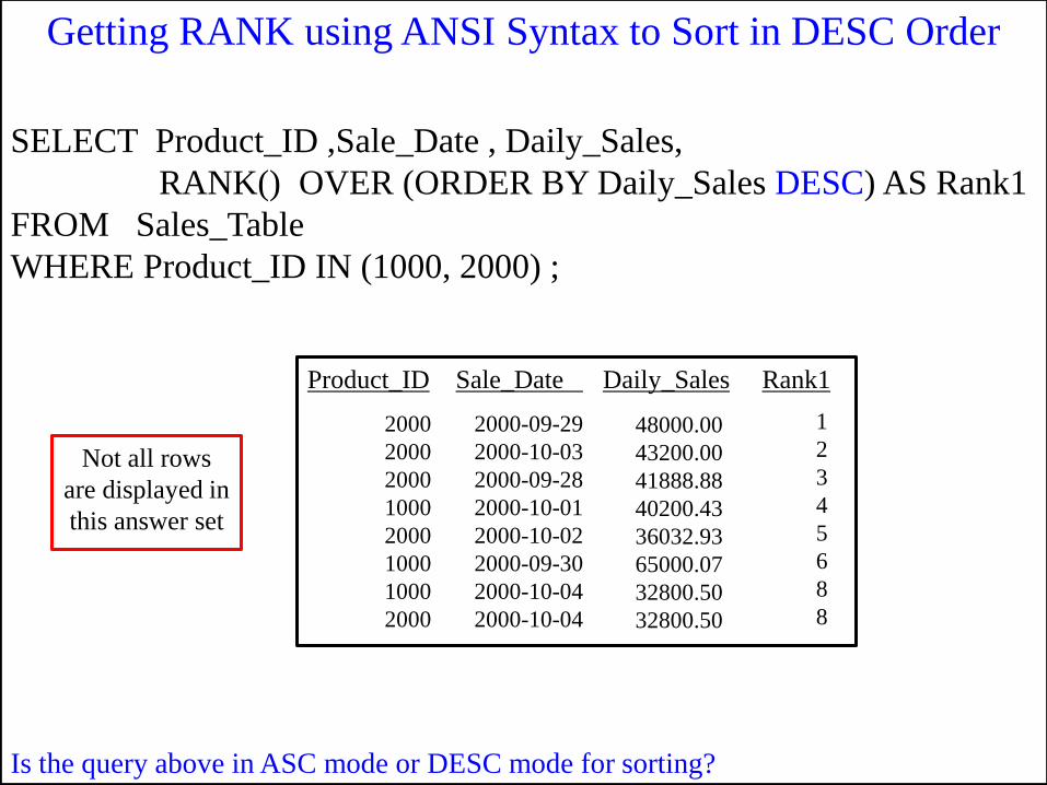
SELECT Product_ID ,Sale_Date , Daily_Sales,
RANK() OVER (ORDER BY Daily_Sales DESC) AS Rank1
FROM Sales_Table
WHERE Product_ID IN (1000, 2000) ;
Is the query above in ASC mode or DESC mode for sorting?
Product_ID Sale_Date Daily_Sales Rank1
2000
2000
2000
1000
2000
1000
1000
2000
2000-09-29
2000-10-03
2000-09-28
2000-10-01
2000-10-02
2000-09-30
2000-10-04
2000-10-04
48000.00
43200.00
41888.88
40200.43
36032.93
65000.07
32800.50
32800.50
1
2
3
4
5
6
8
8
Getting RANK using ANSI Syntax to Sort in DESC Order
Not all rows
are displayed in
this answer set
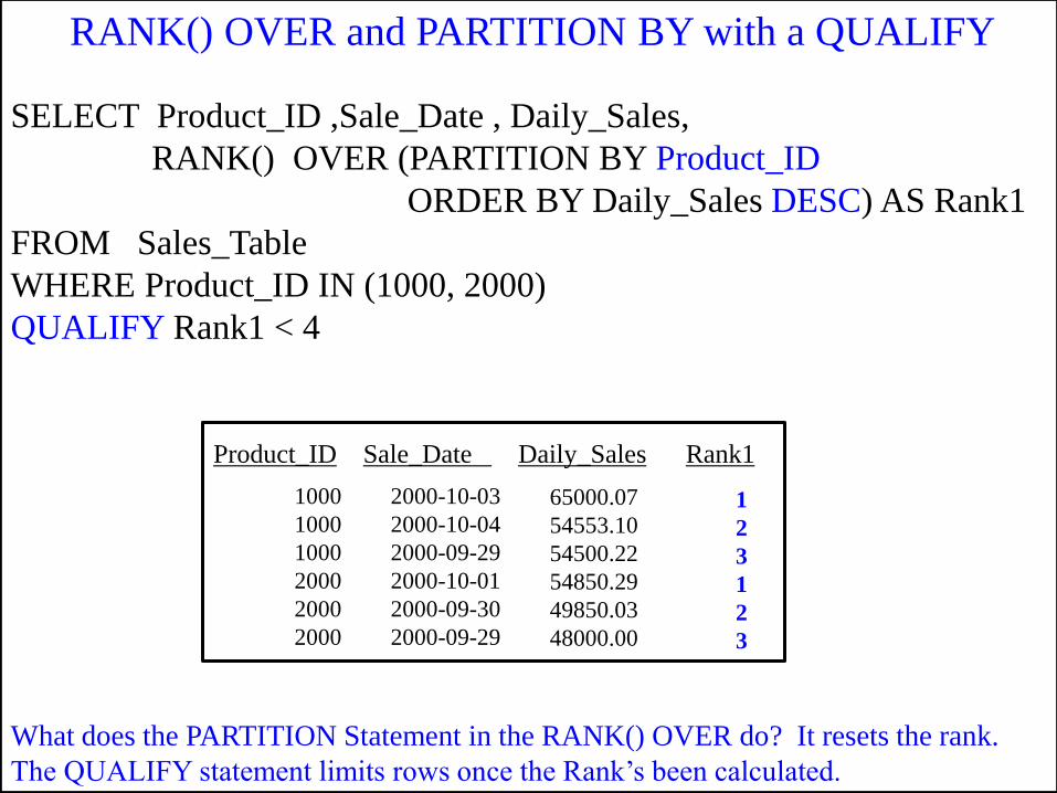
SELECT Product_ID ,Sale_Date , Daily_Sales,
RANK() OVER (PARTITION BY Product_ID
ORDER BY Daily_Sales DESC) AS Rank1
FROM Sales_Table
WHERE Product_ID IN (1000, 2000)
QUALIFY Rank1 < 4
Product_ID Sale_Date Daily_Sales Rank1
What does the PARTITION Statement in the RANK() OVER do? It resets the rank.
The QUALIFY statement limits rows once the Rank‟s been calculated.
RANK() OVER and PARTITION BY with a QUALIFY
1000
1000
1000
2000
2000
2000
2000-10-03
2000-10-04
2000-09-29
2000-10-01
2000-09-30
2000-09-29
65000.07
54553.10
54500.22
54850.29
49850.03
48000.00
1
2
3
1
2
3
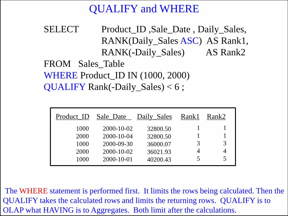
SELECT Product_ID ,Sale_Date , Daily_Sales,
RANK(Daily_Sales ASC) AS Rank1,
RANK(-Daily_Sales) AS Rank2
FROM Sales_Table
WHERE Product_ID IN (1000, 2000)
QUALIFY Rank(-Daily_Sales) < 6 ;
Product_ID Sale_Date Daily_Sales Rank1 Rank2
The WHERE statement is performed first. It limits the rows being calculated. Then the
QUALIFY takes the calculated rows and limits the returning rows. QUALIFY is to
OLAP what HAVING is to Aggregates. Both limit after the calculations.
QUALIFY and WHERE
1000
2000
1000
2000
1000
2000-10-02
2000-10-04
2000-09-30
2000-10-02
2000-10-01
32800.50
32800.50
36000.07
36021.93
40200.43
1
1
3
4
5
1
1
3
4
5
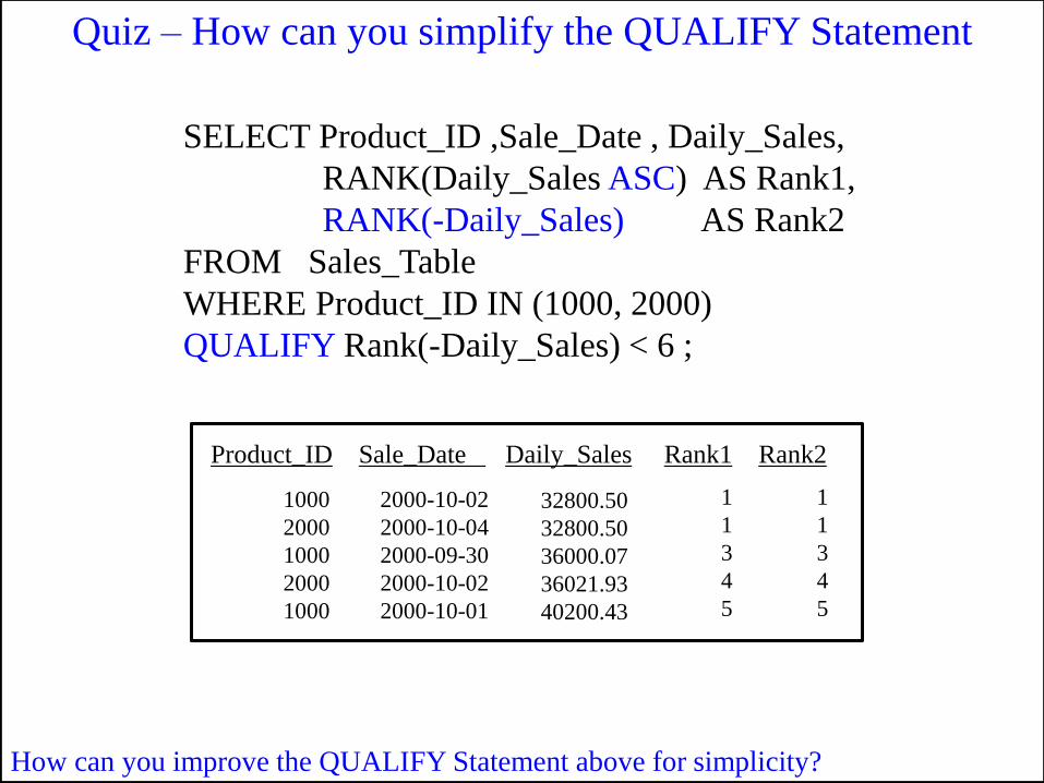
How can you improve the QUALIFY Statement above for simplicity?
SELECT Product_ID ,Sale_Date , Daily_Sales,
RANK(Daily_Sales ASC) AS Rank1,
RANK(-Daily_Sales) AS Rank2
FROM Sales_Table
WHERE Product_ID IN (1000, 2000)
QUALIFY Rank(-Daily_Sales) < 6 ;
Product_ID Sale_Date Daily_Sales Rank1 Rank2
1000
2000
1000
2000
1000
2000-10-02
2000-10-04
2000-09-30
2000-10-02
2000-10-01
32800.50
32800.50
36000.07
36021.93
40200.43
1
1
3
4
5
1
1
3
4
5
Quiz – How can you simplify the QUALIFY Statement
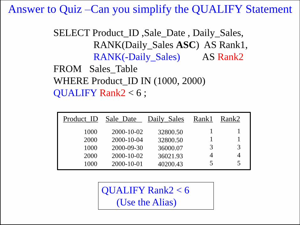
QUALIFY Rank2 < 6
(Use the Alias)
SELECT Product_ID ,Sale_Date , Daily_Sales,
RANK(Daily_Sales ASC) AS Rank1,
RANK(-Daily_Sales) AS Rank2
FROM Sales_Table
WHERE Product_ID IN (1000, 2000)
QUALIFY Rank2 < 6 ;
Product_ID Sale_Date Daily_Sales Rank1 Rank2
1000
2000
1000
2000
1000
2000-10-02
2000-10-04
2000-09-30
2000-10-02
2000-10-01
32800.50
32800.50
36000.07
36021.93
40200.43
1
1
3
4
5
1
1
3
4
5
Answer to Quiz –Can you simplify the QUALIFY Statement
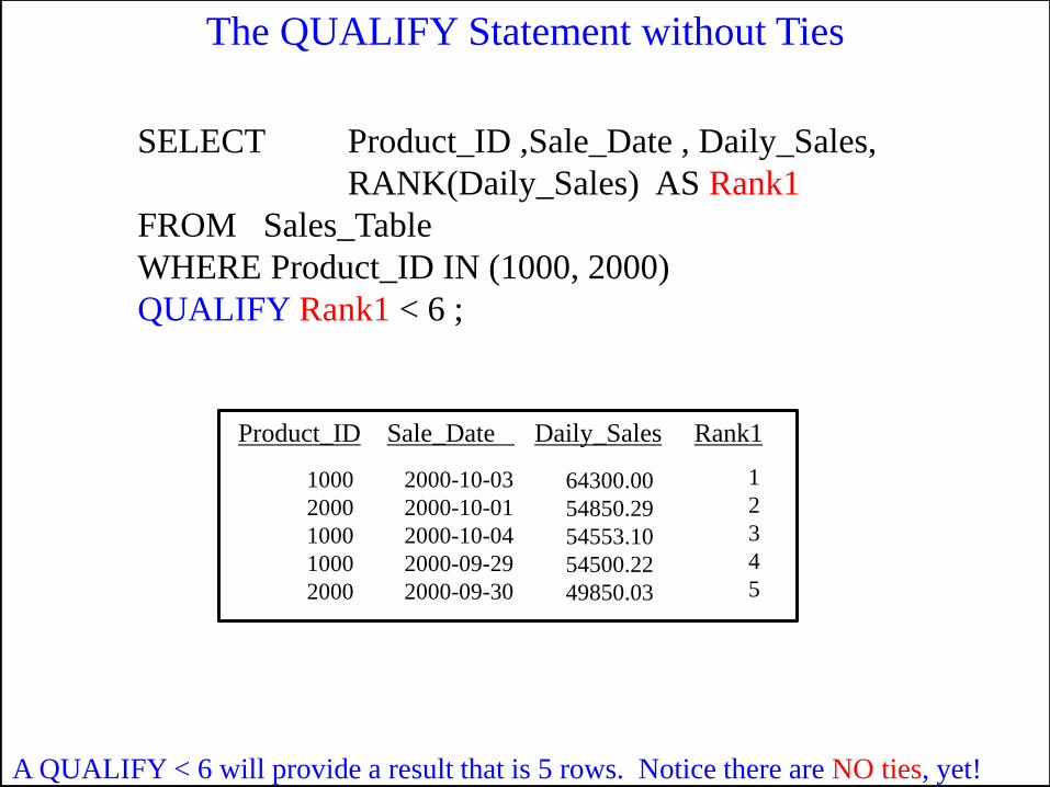
SELECT Product_ID ,Sale_Date , Daily_Sales,
RANK(Daily_Sales) AS Rank1
FROM Sales_Table
WHERE Product_ID IN (1000, 2000)
QUALIFY Rank1 < 6 ;
Product_ID Sale_Date Daily_Sales Rank1
A QUALIFY < 6 will provide a result that is 5 rows. Notice there are NO ties, yet!
1000
2000
1000
1000
2000
2000-10-03
2000-10-01
2000-10-04
2000-09-29
2000-09-30
64300.00
54850.29
54553.10
54500.22
49850.03
1
2
3
4
5
The QUALIFY Statement without Ties
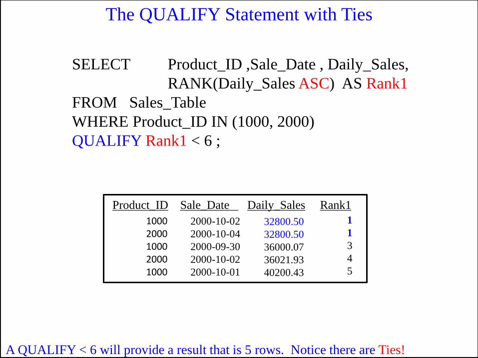
SELECT Product_ID ,Sale_Date , Daily_Sales,
RANK(Daily_Sales ASC) AS Rank1
FROM Sales_Table
WHERE Product_ID IN (1000, 2000)
QUALIFY Rank1 < 6 ;
Product_ID Sale_Date Daily_Sales Rank1
A QUALIFY < 6 will provide a result that is 5 rows. Notice there are Ties!
10002000100020001000
2000-10-02
2000-10-04
2000-09-30
2000-10-02
2000-10-01
32800.50
32800.50
36000.07
36021.93
40200.43
1
1
3
4
5
The QUALIFY Statement with Ties
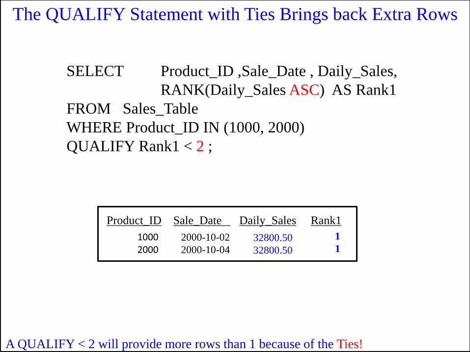
SELECT Product_ID ,Sale_Date , Daily_Sales,
RANK(Daily_Sales ASC) AS Rank1
FROM Sales_Table
WHERE Product_ID IN (1000, 2000)
QUALIFY Rank1 < 2 ;
Product_ID Sale_Date Daily_Sales Rank1
A QUALIFY < 2 will provide more rows than 1 because of the Ties!
10002000
2000-10-02
2000-10-04
32800.50
32800.50
1
1
The QUALIFY Statement with Ties Brings back Extra Rows
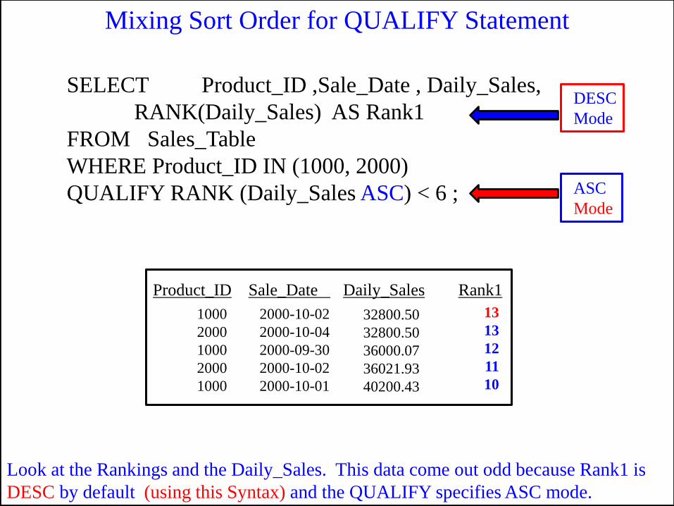
SELECT Product_ID ,Sale_Date , Daily_Sales,
RANK(Daily_Sales) AS Rank1
FROM Sales_Table
WHERE Product_ID IN (1000, 2000)
QUALIFY RANK (Daily_Sales ASC) < 6 ;
Product_ID Sale_Date Daily_Sales Rank1
Look at the Rankings and the Daily_Sales. This data come out odd because Rank1 is
DESC by default (using this Syntax) and the QUALIFY specifies ASC mode.
1000
2000
1000
2000
1000
2000-10-02
2000-10-04
2000-09-30
2000-10-02
2000-10-01
32800.50
32800.50
36000.07
36021.93
40200.43
13
13
12
11
10
DESC
Mode
ASC
Mode
Mixing Sort Order for QUALIFY Statement
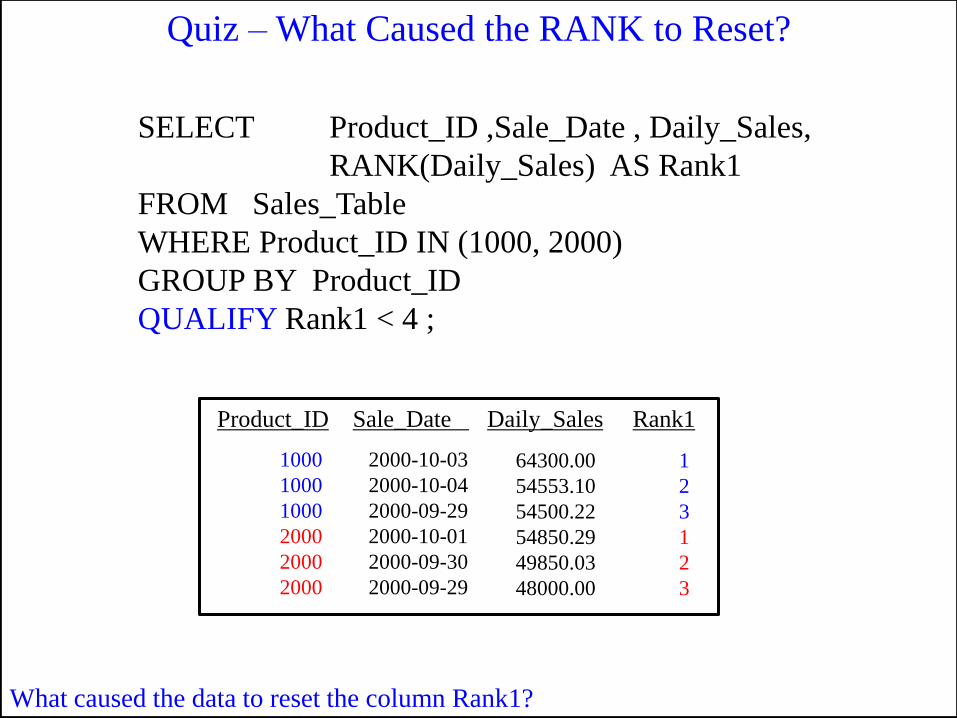
SELECT Product_ID ,Sale_Date , Daily_Sales,
RANK(Daily_Sales) AS Rank1
FROM Sales_Table
WHERE Product_ID IN (1000, 2000)
GROUP BY Product_ID
QUALIFY Rank1 < 4 ;
Product_ID Sale_Date Daily_Sales Rank1
What caused the data to reset the column Rank1?
1000
1000
1000
2000
2000
2000
2000-10-03
2000-10-04
2000-09-29
2000-10-01
2000-09-30
2000-09-29
64300.00
54553.10
54500.22
54850.29
49850.03
48000.00
1
2
3
1
2
3
Quiz – What Caused the RANK to Reset?
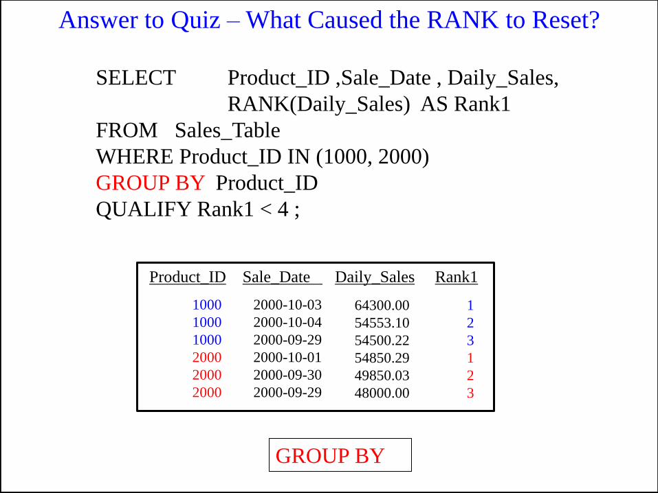
GROUP BY
SELECT Product_ID ,Sale_Date , Daily_Sales,
RANK(Daily_Sales) AS Rank1
FROM Sales_Table
WHERE Product_ID IN (1000, 2000)
GROUP BY Product_ID
QUALIFY Rank1 < 4 ;
Product_ID Sale_Date Daily_Sales Rank1
1000
1000
1000
2000
2000
2000
2000-10-03
2000-10-04
2000-09-29
2000-10-01
2000-09-30
2000-09-29
64300.00
54553.10
54500.22
54850.29
49850.03
48000.00
1
2
3
1
2
3
Answer to Quiz – What Caused the RANK to Reset?
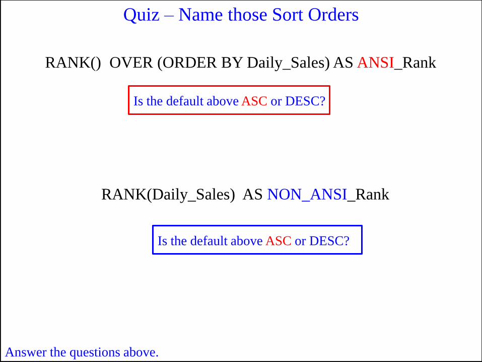
RANK() OVER (ORDER BY Daily_Sales) AS ANSI_Rank
RANK(Daily_Sales) AS NON_ANSI_Rank
Is the default above ASC or DESC?
Is the default above ASC or DESC?
Answer the questions above.
Quiz – Name those Sort Orders
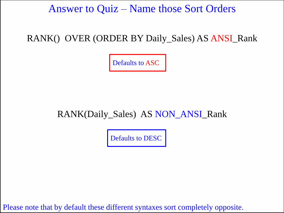
Please note that by default these different syntaxes sort completely opposite.
RANK() OVER (ORDER BY Daily_Sales) AS ANSI_Rank
RANK(Daily_Sales) AS NON_ANSI_Rank
Defaults to ASC
Defaults to DESC
Answer to Quiz – Name those Sort Orders
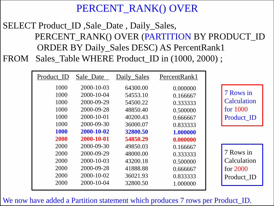
SELECT Product_ID ,Sale_Date , Daily_Sales,
PERCENT_RANK() OVER (PARTITION BY PRODUCT_ID
ORDER BY Daily_Sales DESC) AS PercentRank1
FROM Sales_Table WHERE Product_ID in (1000, 2000) ;
Product_ID Sale_Date Daily_Sales PercentRank1
We now have added a Partition statement which produces 7 rows per Product_ID.
PERCENT_RANK() OVER
1000
1000
1000
1000
1000
1000
1000
2000
2000
2000
2000
2000
2000
2000
2000-10-03
2000-10-04
2000-09-29
2000-09-28
2000-10-01
2000-09-30
2000-10-02
2000-10-01
2000-09-30
2000-09-29
2000-10-03
2000-09-28
2000-10-02
2000-10-04
64300.00
54553.10
54500.22
48850.40
40200.43
36000.07
32800.50
54850.29
49850.03
48000.00
43200.18
41888.88
36021.93
32800.50
0.000000
0.166667
0.333333
0.500000
0.666667
0.833333
1.000000
0.000000
0.166667
0.333333
0.500000
0.666667
0.833333
1.000000
7 Rows in
Calculation
for 1000
Product_ID
7 Rows in
Calculation
for 2000
Product_ID
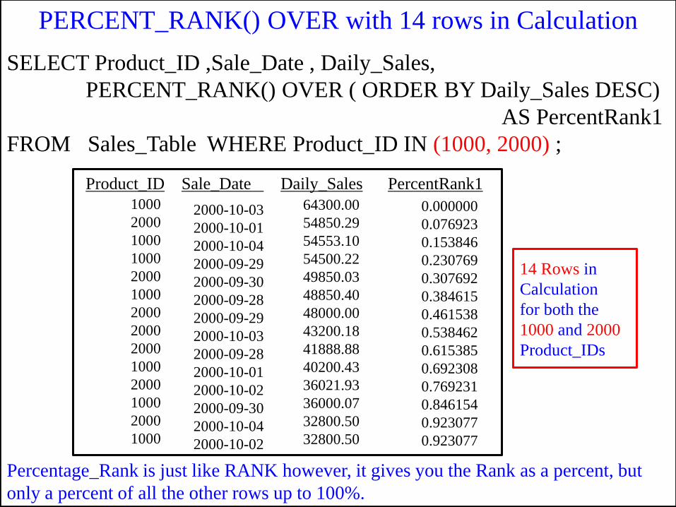
SELECT Product_ID ,Sale_Date , Daily_Sales,
PERCENT_RANK() OVER ( ORDER BY Daily_Sales DESC)
AS PercentRank1
FROM Sales_Table WHERE Product_ID IN (1000, 2000) ;
Product_ID Sale_Date Daily_Sales PercentRank1
Percentage_Rank is just like RANK however, it gives you the Rank as a percent, but
only a percent of all the other rows up to 100%.
1000
2000
1000
1000
2000
1000
2000
2000
2000
1000
2000
1000
2000
1000
2000-10-03
2000-10-01
2000-10-04
2000-09-29
2000-09-30
2000-09-28
2000-09-29
2000-10-03
2000-09-28
2000-10-01
2000-10-02
2000-09-30
2000-10-04
2000-10-02
64300.00
54850.29
54553.10
54500.22
49850.03
48850.40
48000.00
43200.18
41888.88
40200.43
36021.93
36000.07
32800.50
32800.50
0.000000
0.076923
0.153846
0.230769
0.307692
0.384615
0.461538
0.538462
0.615385
0.692308
0.769231
0.846154
0.923077
0.923077
14 Rows in
Calculation
for both the
1000 and 2000
Product_IDs
PERCENT_RANK() OVER with 14 rows in Calculation
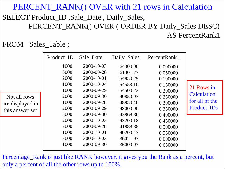
SELECT Product_ID ,Sale_Date , Daily_Sales,
PERCENT_RANK() OVER ( ORDER BY Daily_Sales DESC)
AS PercentRank1
FROM Sales_Table ;
Product_ID Sale_Date Daily_Sales PercentRank1
Percentage_Rank is just like RANK however, it gives you the Rank as a percent, but
only a percent of all the other rows up to 100%.
1000
3000
2000
1000
1000
2000
1000
2000
3000
2000
2000
1000
2000
1000
2000-10-03
2000-09-28
2000-10-01
2000-10-04
2000-09-29
2000-09-30
2000-09-28
2000-09-29
2000-09-30
2000-10-03
2000-09-28
2000-10-01
2000-10-02
2000-09-30
64300.00
61301.77
54850.29
54553.10
54500.22
49850.03
48850.40
48000.00
43868.86
43200.18
41888.88
40200.43
36021.93
36000.07
0.000000
0.050000
0.100000
0.150000
0.200000
0.250000
0.300000
0.350000
0.400000
0.450000
0.500000
0.550000
0.600000
0.650000
21 Rows in
Calculation
for all of the
Product_IDs
PERCENT_RANK() OVER with 21 rows in Calculation
Not all rows
are displayed in
this answer set
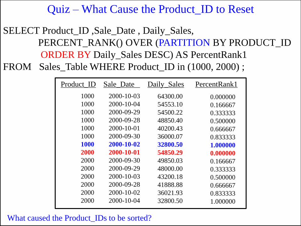
What caused the Product_IDs to be sorted?
SELECT Product_ID ,Sale_Date , Daily_Sales,
PERCENT_RANK() OVER (PARTITION BY PRODUCT_ID
ORDER BY Daily_Sales DESC) AS PercentRank1
FROM Sales_Table WHERE Product_ID in (1000, 2000) ;
Product_ID Sale_Date Daily_Sales PercentRank1
1000
1000
1000
1000
1000
1000
1000
2000
2000
2000
2000
2000
2000
2000
2000-10-03
2000-10-04
2000-09-29
2000-09-28
2000-10-01
2000-09-30
2000-10-02
2000-10-01
2000-09-30
2000-09-29
2000-10-03
2000-09-28
2000-10-02
2000-10-04
64300.00
54553.10
54500.22
48850.40
40200.43
36000.07
32800.50
54850.29
49850.03
48000.00
43200.18
41888.88
36021.93
32800.50
0.000000
0.166667
0.333333
0.500000
0.666667
0.833333
1.000000
0.000000
0.166667
0.333333
0.500000
0.666667
0.833333
1.000000
Quiz – What Cause the Product_ID to Reset
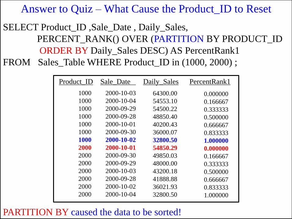
PARTITION BY caused the data to be sorted!
SELECT Product_ID ,Sale_Date , Daily_Sales,
PERCENT_RANK() OVER (PARTITION BY PRODUCT_ID
ORDER BY Daily_Sales DESC) AS PercentRank1
FROM Sales_Table WHERE Product_ID in (1000, 2000) ;
Product_ID Sale_Date Daily_Sales PercentRank1
1000
1000
1000
1000
1000
1000
1000
2000
2000
2000
2000
2000
2000
2000
2000-10-03
2000-10-04
2000-09-29
2000-09-28
2000-10-01
2000-09-30
2000-10-02
2000-10-01
2000-09-30
2000-09-29
2000-10-03
2000-09-28
2000-10-02
2000-10-04
64300.00
54553.10
54500.22
48850.40
40200.43
36000.07
32800.50
54850.29
49850.03
48000.00
43200.18
41888.88
36021.93
32800.50
0.000000
0.166667
0.333333
0.500000
0.666667
0.833333
1.000000
0.000000
0.166667
0.333333
0.500000
0.666667
0.833333
1.000000
Answer to Quiz – What Cause the Product_ID to Reset
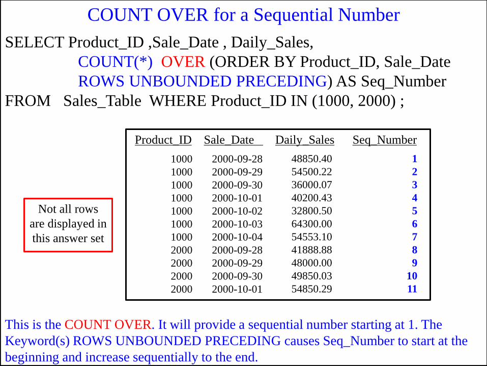
SELECT Product_ID ,Sale_Date , Daily_Sales,
COUNT(*) OVER (ORDER BY Product_ID, Sale_Date
ROWS UNBOUNDED PRECEDING) AS Seq_Number
FROM Sales_Table WHERE Product_ID IN (1000, 2000) ;
Product_ID Sale_Date Daily_Sales Seq_Number
This is the COUNT OVER. It will provide a sequential number starting at 1. The
Keyword(s) ROWS UNBOUNDED PRECEDING causes Seq_Number to start at the
beginning and increase sequentially to the end.
1000
1000
1000
1000
1000
1000
1000
2000
2000
2000
2000
2000-09-28
2000-09-29
2000-09-30
2000-10-01
2000-10-02
2000-10-03
2000-10-04
2000-09-28
2000-09-29
2000-09-30
2000-10-01
48850.40
54500.22
36000.07
40200.43
32800.50
64300.00
54553.10
41888.88
48000.00
49850.03
54850.29
1
2
3
4
5
6
7
8
9
10
11
COUNT OVER for a Sequential Number
Not all rows
are displayed in
this answer set
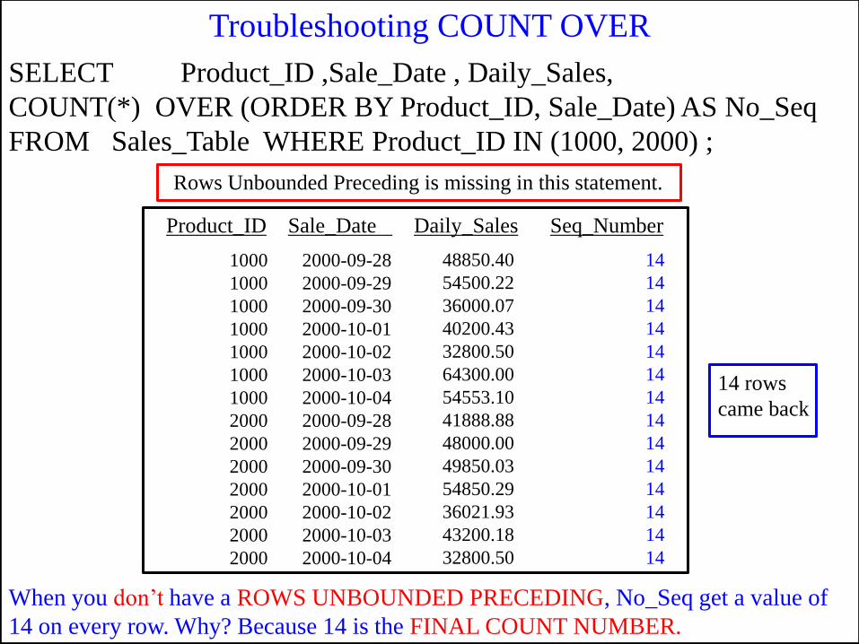
Product_ID Sale_Date Daily_Sales Seq_Number
1000
1000
1000
1000
1000
1000
1000
2000
2000
2000
2000
2000
2000
2000
2000-09-28
2000-09-29
2000-09-30
2000-10-01
2000-10-02
2000-10-03
2000-10-04
2000-09-28
2000-09-29
2000-09-30
2000-10-01
2000-10-02
2000-10-03
2000-10-04
48850.40
54500.22
36000.07
40200.43
32800.50
64300.00
54553.10
41888.88
48000.00
49850.03
54850.29
36021.93
43200.18
32800.50
14
14
14
14
14
14
14
14
14
14
14
14
14
14
SELECT Product_ID ,Sale_Date , Daily_Sales,
COUNT(*) OVER (ORDER BY Product_ID, Sale_Date) AS No_Seq
FROM Sales_Table WHERE Product_ID IN (1000, 2000) ;
When you don‟t have a ROWS UNBOUNDED PRECEDING, No_Seq get a value of
14 on every row. Why? Because 14 is the FINAL COUNT NUMBER.
Rows Unbounded Preceding is missing in this statement.
Troubleshooting COUNT OVER
14 rows
came back
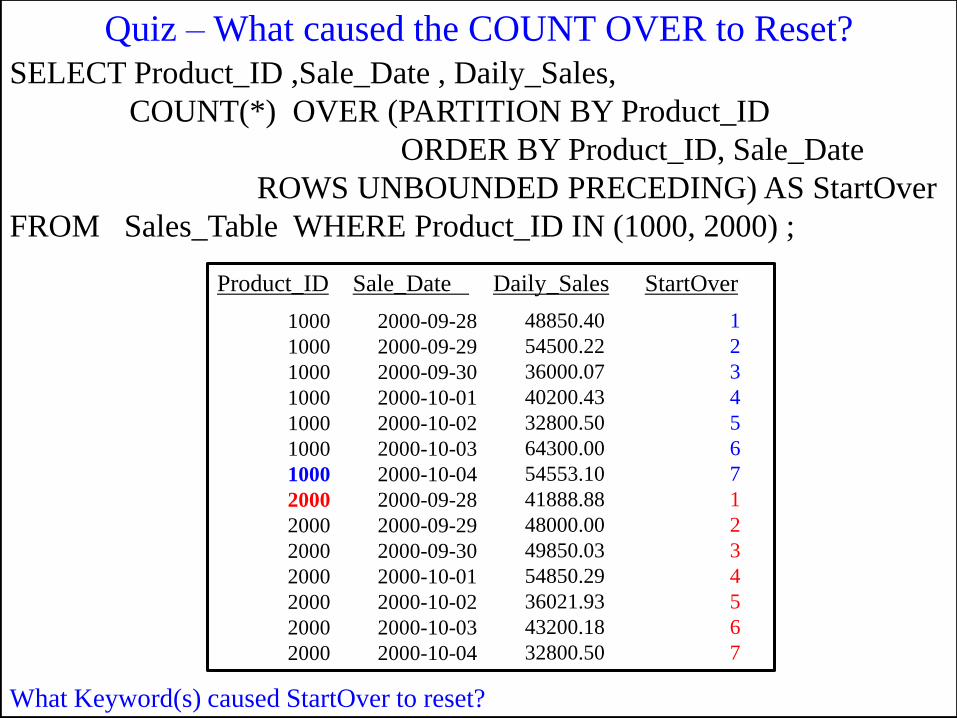
SELECT Product_ID ,Sale_Date , Daily_Sales,
COUNT(*) OVER (PARTITION BY Product_ID
ORDER BY Product_ID, Sale_Date
ROWS UNBOUNDED PRECEDING) AS StartOver
FROM Sales_Table WHERE Product_ID IN (1000, 2000) ;
Product_ID Sale_Date Daily_Sales StartOver
What Keyword(s) caused StartOver to reset?
1000
1000
1000
1000
1000
1000
1000
2000
2000
2000
2000
2000
2000
2000
2000-09-28
2000-09-29
2000-09-30
2000-10-01
2000-10-02
2000-10-03
2000-10-04
2000-09-28
2000-09-29
2000-09-30
2000-10-01
2000-10-02
2000-10-03
2000-10-04
48850.40
54500.22
36000.07
40200.43
32800.50
64300.00
54553.10
41888.88
48000.00
49850.03
54850.29
36021.93
43200.18
32800.50
1
2
3
4
5
6
7
1
2
3
4
5
6
7
Quiz – What caused the COUNT OVER to Reset?
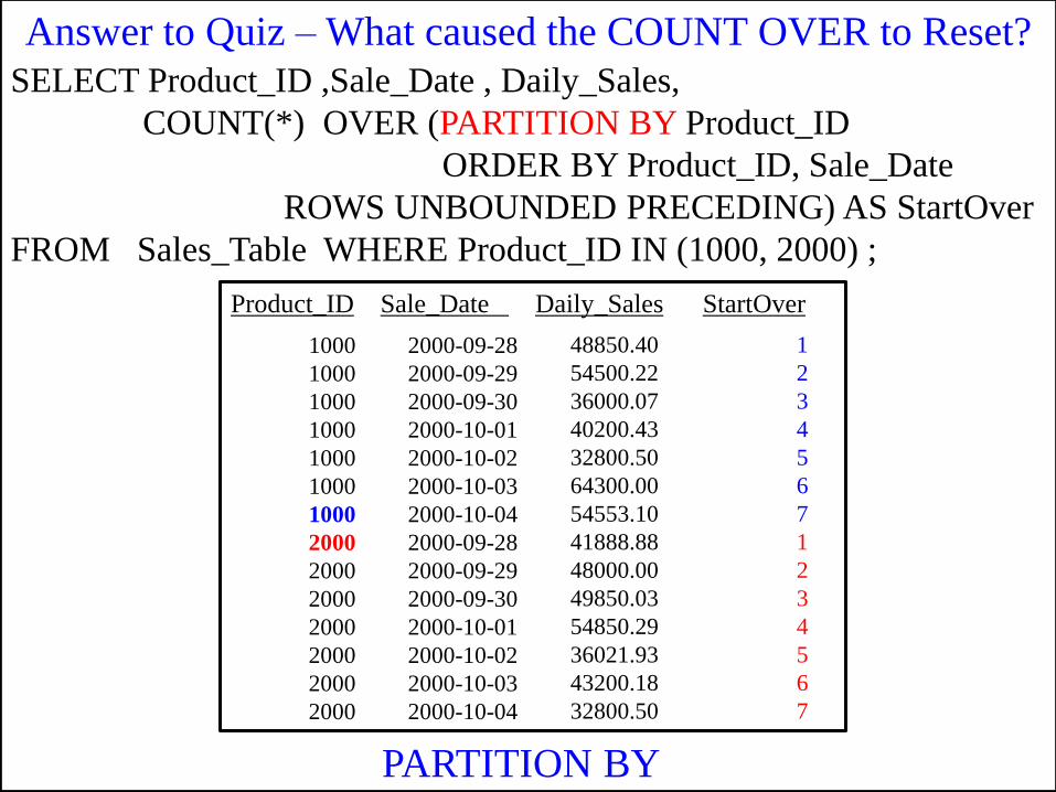
PARTITION BY
SELECT Product_ID ,Sale_Date , Daily_Sales,
COUNT(*) OVER (PARTITION BY Product_ID
ORDER BY Product_ID, Sale_Date
ROWS UNBOUNDED PRECEDING) AS StartOver
FROM Sales_Table WHERE Product_ID IN (1000, 2000) ;
Product_ID Sale_Date Daily_Sales StartOver
1000
1000
1000
1000
1000
1000
1000
2000
2000
2000
2000
2000
2000
2000
2000-09-28
2000-09-29
2000-09-30
2000-10-01
2000-10-02
2000-10-03
2000-10-04
2000-09-28
2000-09-29
2000-09-30
2000-10-01
2000-10-02
2000-10-03
2000-10-04
48850.40
54500.22
36000.07
40200.43
32800.50
64300.00
54553.10
41888.88
48000.00
49850.03
54850.29
36021.93
43200.18
32800.50
1
2
3
4
5
6
7
1
2
3
4
5
6
7
Answer to Quiz – What caused the COUNT OVER to Reset?
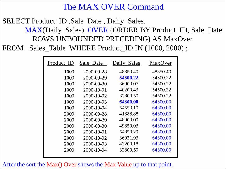
SELECT Product_ID ,Sale_Date , Daily_Sales,
MAX(Daily_Sales) OVER (ORDER BY Product_ID, Sale_Date
ROWS UNBOUNDED PRECEDING) AS MaxOver
FROM Sales_Table WHERE Product_ID IN (1000, 2000) ;
Product_ID Sale_Date Daily_Sales MaxOver
After the sort the Max() Over shows the Max Value up to that point.
1000
1000
1000
1000
1000
1000
1000
2000
2000
2000
2000
2000
2000
2000
2000-09-28
2000-09-29
2000-09-30
2000-10-01
2000-10-02
2000-10-03
2000-10-04
2000-09-28
2000-09-29
2000-09-30
2000-10-01
2000-10-02
2000-10-03
2000-10-04
48850.40
54500.22
36000.07
40200.43
32800.50
64300.00
54553.10
41888.88
48000.00
49850.03
54850.29
36021.93
43200.18
32800.50
48850.40
54500.22
54500.22
54500.22
54500.22
64300.00
64300.00
64300.00
64300.00
64300.00
64300.00
64300.00
64300.00
64300.00
The MAX OVER Command
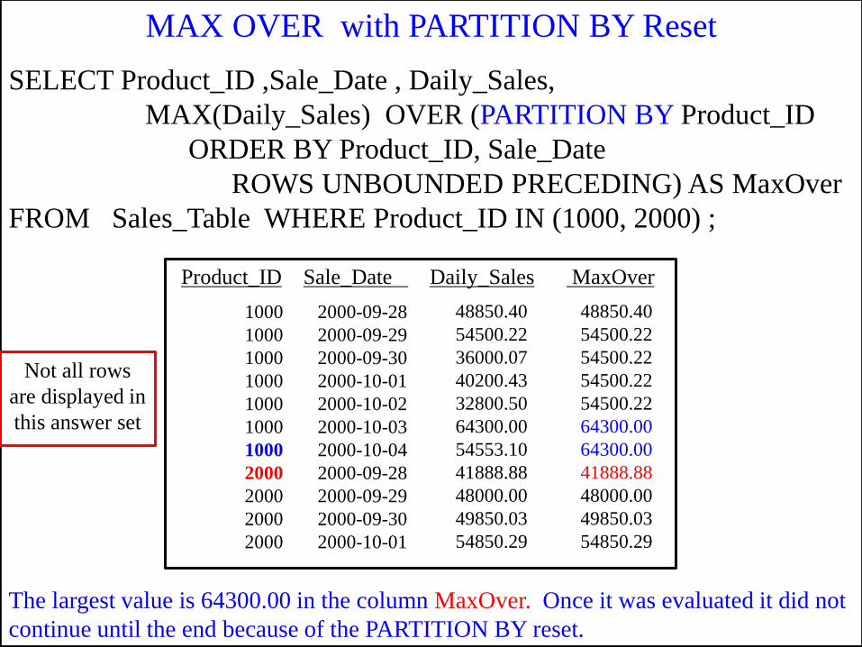
SELECT Product_ID ,Sale_Date , Daily_Sales,
MAX(Daily_Sales) OVER (PARTITION BY Product_ID
ORDER BY Product_ID, Sale_Date
ROWS UNBOUNDED PRECEDING) AS MaxOver
FROM Sales_Table WHERE Product_ID IN (1000, 2000) ;
Product_ID Sale_Date Daily_Sales MaxOver
The largest value is 64300.00 in the column MaxOver. Once it was evaluated it did not
continue until the end because of the PARTITION BY reset.
1000
1000
1000
1000
1000
1000
1000
2000
2000
2000
2000
2000-09-28
2000-09-29
2000-09-30
2000-10-01
2000-10-02
2000-10-03
2000-10-04
2000-09-28
2000-09-29
2000-09-30
2000-10-01
48850.40
54500.22
36000.07
40200.43
32800.50
64300.00
54553.10
41888.88
48000.00
49850.03
54850.29
48850.40
54500.22
54500.22
54500.22
54500.22
64300.00
64300.00
41888.88
48000.00
49850.03
54850.29
MAX OVER with PARTITION BY Reset
Not all rows
are displayed in
this answer set
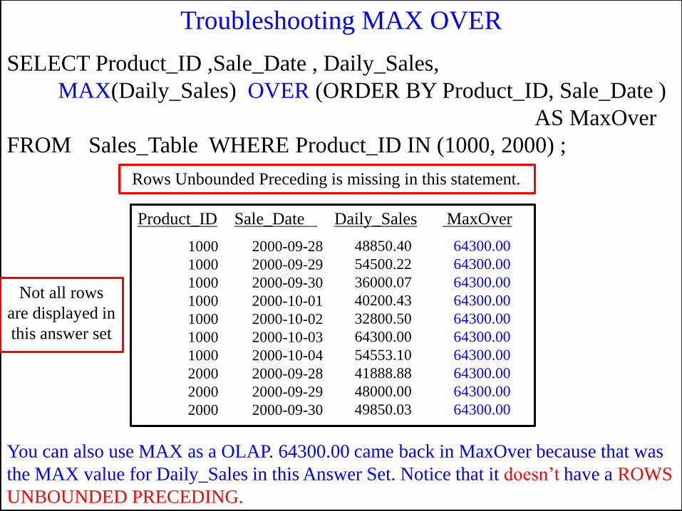
SELECT Product_ID ,Sale_Date , Daily_Sales,
MAX(Daily_Sales) OVER (ORDER BY Product_ID, Sale_Date )
AS MaxOver
FROM Sales_Table WHERE Product_ID IN (1000, 2000) ;
Product_ID Sale_Date Daily_Sales MaxOver
You can also use MAX as a OLAP. 64300.00 came back in MaxOver because that was
the MAX value for Daily_Sales in this Answer Set. Notice that it doesn‟t have a ROWS
UNBOUNDED PRECEDING.
1000
1000
1000
1000
1000
1000
1000
2000
2000
2000
2000-09-28
2000-09-29
2000-09-30
2000-10-01
2000-10-02
2000-10-03
2000-10-04
2000-09-28
2000-09-29
2000-09-30
48850.40
54500.22
36000.07
40200.43
32800.50
64300.00
54553.10
41888.88
48000.00
49850.03
64300.00
64300.00
64300.00
64300.00
64300.00
64300.00
64300.00
64300.00
64300.00
64300.00
Troubleshooting MAX OVER
Rows Unbounded Preceding is missing in this statement.
Not all rows
are displayed in
this answer set
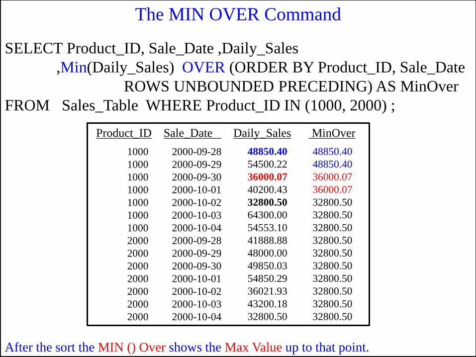
SELECT Product_ID, Sale_Date ,Daily_Sales
,Min(Daily_Sales) OVER (ORDER BY Product_ID, Sale_Date
ROWS UNBOUNDED PRECEDING) AS MinOver
FROM Sales_Table WHERE Product_ID IN (1000, 2000) ;
Product_ID Sale_Date Daily_Sales MinOver
1000
1000
1000
1000
1000
1000
1000
2000
2000
2000
2000
2000
2000
2000
2000-09-28
2000-09-29
2000-09-30
2000-10-01
2000-10-02
2000-10-03
2000-10-04
2000-09-28
2000-09-29
2000-09-30
2000-10-01
2000-10-02
2000-10-03
2000-10-04
48850.40
54500.22
36000.07
40200.43
32800.50
64300.00
54553.10
41888.88
48000.00
49850.03
54850.29
36021.93
43200.18
32800.50
48850.40
48850.40
36000.07
36000.07
32800.50
32800.50
32800.50
32800.50
32800.50
32800.50
32800.50
32800.50
32800.50
32800.50
After the sort the MIN () Over shows the Max Value up to that point.
The MIN OVER Command
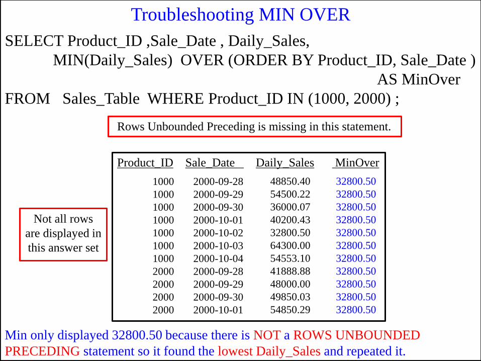
SELECT Product_ID ,Sale_Date , Daily_Sales,
MIN(Daily_Sales) OVER (ORDER BY Product_ID, Sale_Date )
AS MinOver
FROM Sales_Table WHERE Product_ID IN (1000, 2000) ;
Product_ID Sale_Date Daily_Sales MinOver
Min only displayed 32800.50 because there is NOT a ROWS UNBOUNDED
PRECEDING statement so it found the lowest Daily_Sales and repeated it.
1000
1000
1000
1000
1000
1000
1000
2000
2000
2000
2000
2000-09-28
2000-09-29
2000-09-30
2000-10-01
2000-10-02
2000-10-03
2000-10-04
2000-09-28
2000-09-29
2000-09-30
2000-10-01
48850.40
54500.22
36000.07
40200.43
32800.50
64300.00
54553.10
41888.88
48000.00
49850.03
54850.29
32800.50
32800.50
32800.50
32800.50
32800.50
32800.50
32800.50
32800.50
32800.50
32800.50
32800.50
Troubleshooting MIN OVER
Rows Unbounded Preceding is missing in this statement.
Not all rows
are displayed in
this answer set
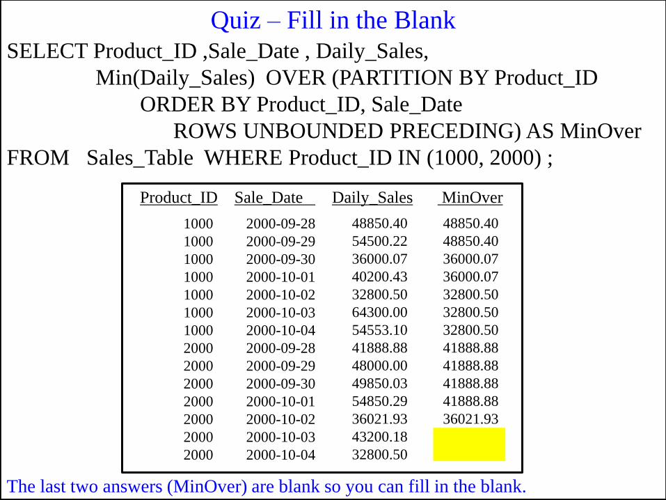
SELECT Product_ID ,Sale_Date , Daily_Sales,
Min(Daily_Sales) OVER (PARTITION BY Product_ID
ORDER BY Product_ID, Sale_Date
ROWS UNBOUNDED PRECEDING) AS MinOver
FROM Sales_Table WHERE Product_ID IN (1000, 2000) ;
Product_ID Sale_Date Daily_Sales MinOver
The last two answers (MinOver) are blank so you can fill in the blank.
1000
1000
1000
1000
1000
1000
1000
2000
2000
2000
2000
2000
2000
2000
2000-09-28
2000-09-29
2000-09-30
2000-10-01
2000-10-02
2000-10-03
2000-10-04
2000-09-28
2000-09-29
2000-09-30
2000-10-01
2000-10-02
2000-10-03
2000-10-04
48850.40
54500.22
36000.07
40200.43
32800.50
64300.00
54553.10
41888.88
48000.00
49850.03
54850.29
36021.93
43200.18
32800.50
48850.40
48850.40
36000.07
36000.07
32800.50
32800.50
32800.50
41888.88
41888.88
41888.88
41888.88
36021.93
Quiz – Fill in the Blank
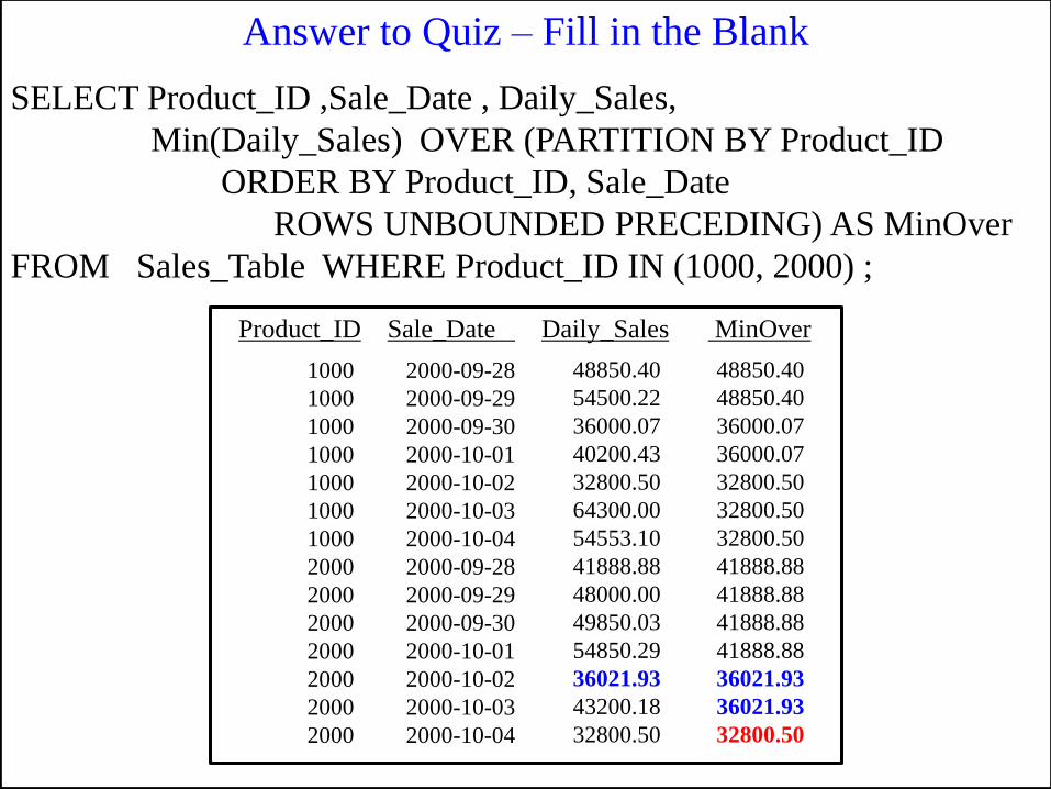
SELECT Product_ID ,Sale_Date , Daily_Sales,
Min(Daily_Sales) OVER (PARTITION BY Product_ID
ORDER BY Product_ID, Sale_Date
ROWS UNBOUNDED PRECEDING) AS MinOver
FROM Sales_Table WHERE Product_ID IN (1000, 2000) ;
Product_ID Sale_Date Daily_Sales MinOver
1000
1000
1000
1000
1000
1000
1000
2000
2000
2000
2000
2000
2000
2000
2000-09-28
2000-09-29
2000-09-30
2000-10-01
2000-10-02
2000-10-03
2000-10-04
2000-09-28
2000-09-29
2000-09-30
2000-10-01
2000-10-02
2000-10-03
2000-10-04
48850.40
54500.22
36000.07
40200.43
32800.50
64300.00
54553.10
41888.88
48000.00
49850.03
54850.29
36021.93
43200.18
32800.50
48850.40
48850.40
36000.07
36000.07
32800.50
32800.50
32800.50
41888.88
41888.88
41888.88
41888.88
36021.93
36021.93
32800.50
Answer to Quiz – Fill in the Blank
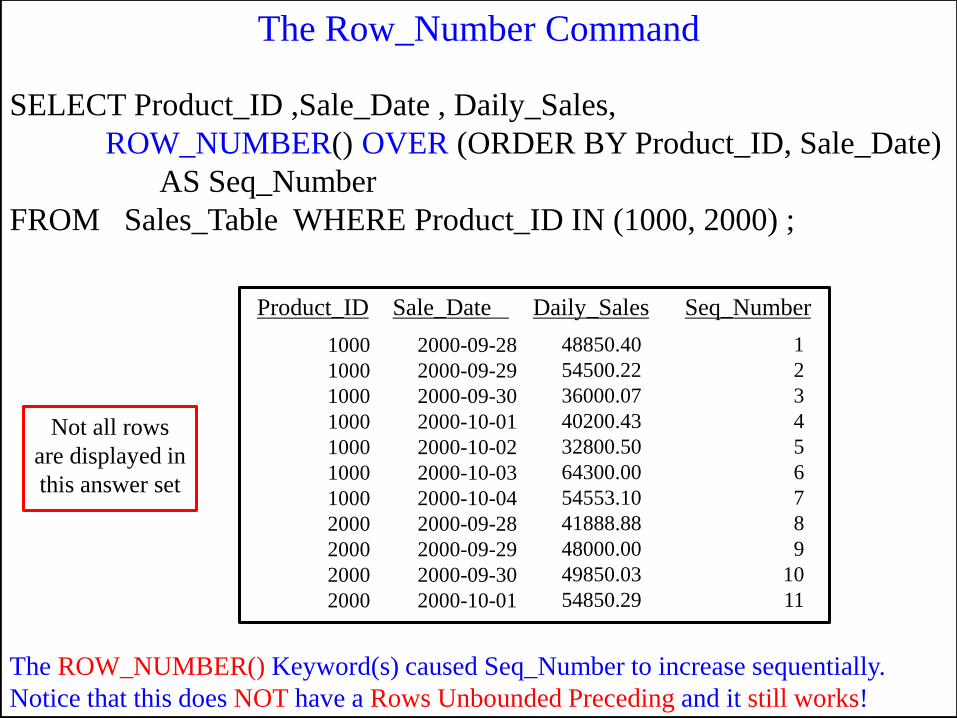
SELECT Product_ID ,Sale_Date , Daily_Sales,
ROW_NUMBER() OVER (ORDER BY Product_ID, Sale_Date)
AS Seq_Number
FROM Sales_Table WHERE Product_ID IN (1000, 2000) ;
Product_ID Sale_Date Daily_Sales Seq_Number
The ROW_NUMBER() Keyword(s) caused Seq_Number to increase sequentially.
Notice that this does NOT have a Rows Unbounded Preceding and it still works!
1000
1000
1000
1000
1000
1000
1000
2000
2000
2000
2000
2000-09-28
2000-09-29
2000-09-30
2000-10-01
2000-10-02
2000-10-03
2000-10-04
2000-09-28
2000-09-29
2000-09-30
2000-10-01
48850.40
54500.22
36000.07
40200.43
32800.50
64300.00
54553.10
41888.88
48000.00
49850.03
54850.29
1
2
3
4
5
6
7
8
9
10
11
Not all rows
are displayed in
this answer set
The Row_Number Command
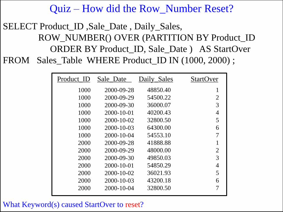
Product_ID Sale_Date Daily_Sales StartOver
1000
1000
1000
1000
1000
1000
1000
2000
2000
2000
2000
2000
2000
2000
2000-09-28
2000-09-29
2000-09-30
2000-10-01
2000-10-02
2000-10-03
2000-10-04
2000-09-28
2000-09-29
2000-09-30
2000-10-01
2000-10-02
2000-10-03
2000-10-04
48850.40
54500.22
36000.07
40200.43
32800.50
64300.00
54553.10
41888.88
48000.00
49850.03
54850.29
36021.93
43200.18
32800.50
1
2
3
4
5
6
7
1
2
3
4
5
6
7
SELECT Product_ID ,Sale_Date , Daily_Sales,
ROW_NUMBER() OVER (PARTITION BY Product_ID
ORDER BY Product_ID, Sale_Date ) AS StartOver
FROM Sales_Table WHERE Product_ID IN (1000, 2000) ;
What Keyword(s) caused StartOver to reset?
Quiz – How did the Row_Number Reset?
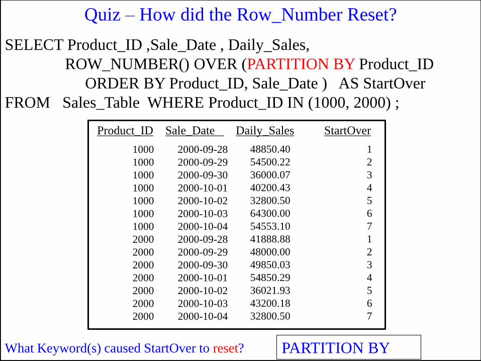
Product_ID Sale_Date Daily_Sales StartOver
1000
1000
1000
1000
1000
1000
1000
2000
2000
2000
2000
2000
2000
2000
2000-09-28
2000-09-29
2000-09-30
2000-10-01
2000-10-02
2000-10-03
2000-10-04
2000-09-28
2000-09-29
2000-09-30
2000-10-01
2000-10-02
2000-10-03
2000-10-04
48850.40
54500.22
36000.07
40200.43
32800.50
64300.00
54553.10
41888.88
48000.00
49850.03
54850.29
36021.93
43200.18
32800.50
1
2
3
4
5
6
7
1
2
3
4
5
6
7
SELECT Product_ID ,Sale_Date , Daily_Sales,
ROW_NUMBER() OVER (PARTITION BY Product_ID
ORDER BY Product_ID, Sale_Date ) AS StartOver
FROM Sales_Table WHERE Product_ID IN (1000, 2000) ;
What Keyword(s) caused StartOver to reset? PARTITION BY
Quiz – How did the Row_Number Reset?
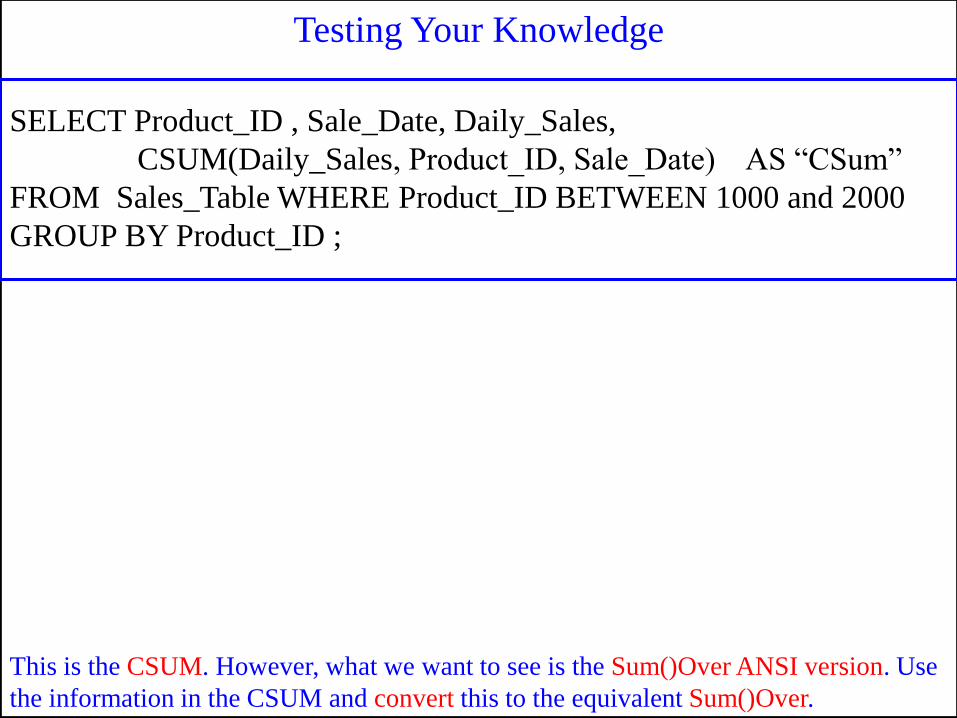
This is the CSUM. However, what we want to see is the Sum()Over ANSI version. Use
the information in the CSUM and convert this to the equivalent Sum()Over.
SELECT Product_ID , Sale_Date, Daily_Sales,
CSUM(Daily_Sales, Product_ID, Sale_Date) AS “CSum”
FROM Sales_Table WHERE Product_ID BETWEEN 1000 and 2000
GROUP BY Product_ID ;
Testing Your Knowledge
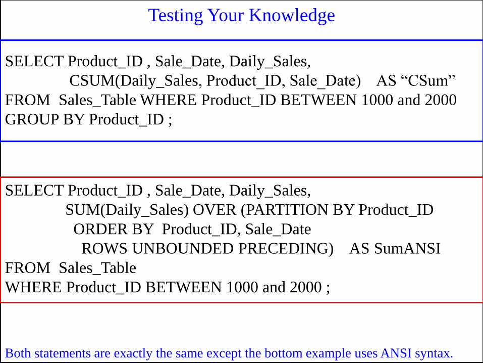
Both statements are exactly the same except the bottom example uses ANSI syntax.
SELECT Product_ID , Sale_Date, Daily_Sales,
CSUM(Daily_Sales, Product_ID, Sale_Date) AS “CSum”
FROM Sales_Table WHERE Product_ID BETWEEN 1000 and 2000
GROUP BY Product_ID ;
Testing Your Knowledge
SELECT Product_ID , Sale_Date, Daily_Sales,
SUM(Daily_Sales) OVER (PARTITION BY Product_ID
ORDER BY Product_ID, Sale_Date
ROWS UNBOUNDED PRECEDING) AS SumANSI
FROM Sales_Table
WHERE Product_ID BETWEEN 1000 and 2000 ;
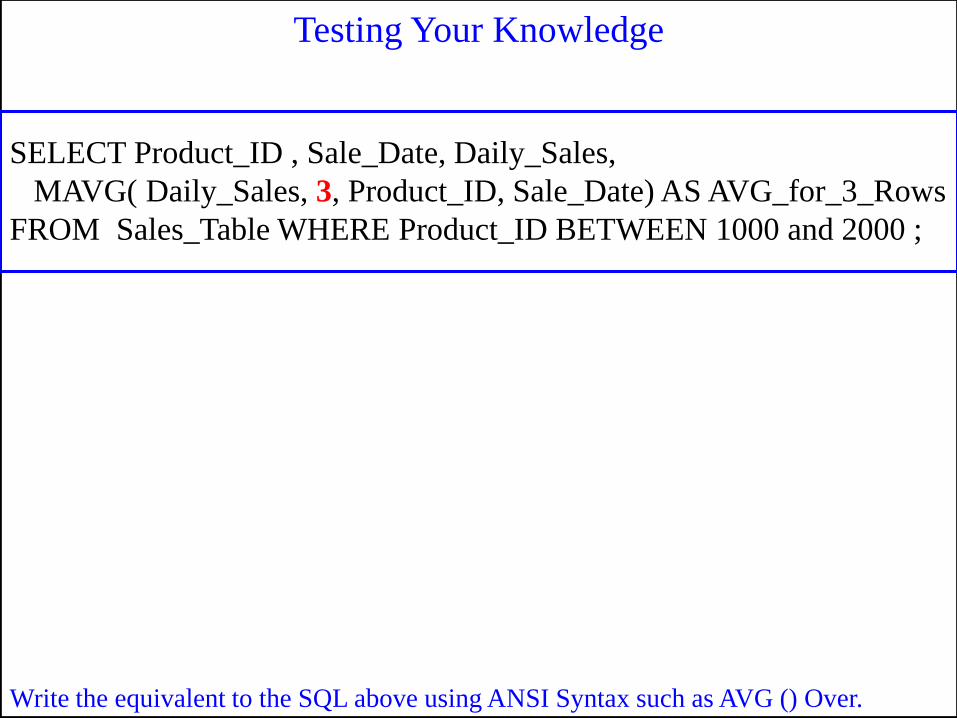
SELECT Product_ID , Sale_Date, Daily_Sales,
MAVG( Daily_Sales, 3, Product_ID, Sale_Date) AS AVG_for_3_Rows
FROM Sales_Table WHERE Product_ID BETWEEN 1000 and 2000 ;
Write the equivalent to the SQL above using ANSI Syntax such as AVG () Over.
Testing Your Knowledge
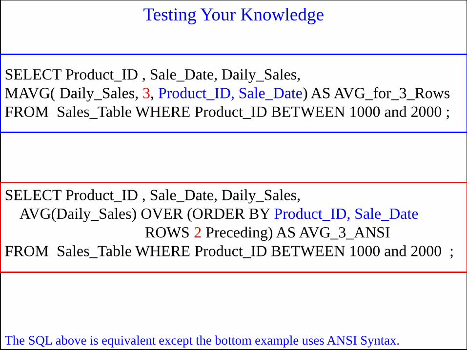
SELECT Product_ID , Sale_Date, Daily_Sales,
MAVG( Daily_Sales, 3, Product_ID, Sale_Date) AS AVG_for_3_Rows
FROM Sales_Table WHERE Product_ID BETWEEN 1000 and 2000 ;
The SQL above is equivalent except the bottom example uses ANSI Syntax.
Testing Your Knowledge
SELECT Product_ID , Sale_Date, Daily_Sales,
AVG(Daily_Sales) OVER (ORDER BY Product_ID, Sale_Date
ROWS 2 Preceding) AS AVG_3_ANSI
FROM Sales_Table WHERE Product_ID BETWEEN 1000 and 2000 ;
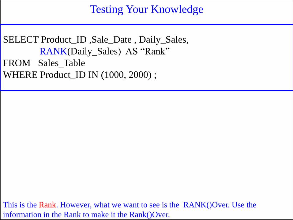
SELECT Product_ID ,Sale_Date , Daily_Sales,
RANK(Daily_Sales) AS “Rank”
FROM Sales_Table
WHERE Product_ID IN (1000, 2000) ;
Testing Your Knowledge
This is the Rank. However, what we want to see is the RANK()Over. Use the
information in the Rank to make it the Rank()Over.
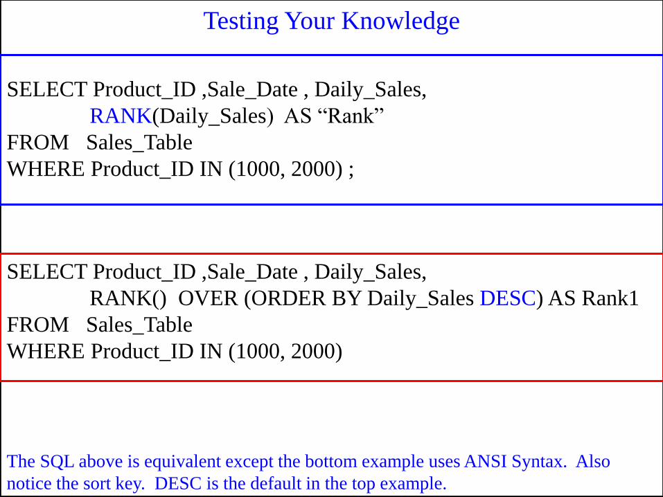
SELECT Product_ID ,Sale_Date , Daily_Sales,
RANK(Daily_Sales) AS “Rank”
FROM Sales_Table
WHERE Product_ID IN (1000, 2000) ;
Testing Your Knowledge
SELECT Product_ID ,Sale_Date , Daily_Sales,
RANK() OVER (ORDER BY Daily_Sales DESC) AS Rank1
FROM Sales_Table
WHERE Product_ID IN (1000, 2000)
The SQL above is equivalent except the bottom example uses ANSI Syntax. Also
notice the sort key. DESC is the default in the top example.