Embed Size (px)
Citation preview

Tensors of low rank
Horobet, E.
Published: 19/05/2016
Document VersionPublisher’s PDF, also known as Version of Record (includes final page, issue and volume numbers)
Please check the document version of this publication:
• A submitted manuscript is the author's version of the article upon submission and before peer-review. There can be important differencesbetween the submitted version and the official published version of record. People interested in the research are advised to contact theauthor for the final version of the publication, or visit the DOI to the publisher's website.• The final author version and the galley proof are versions of the publication after peer review.• The final published version features the final layout of the paper including the volume, issue and page numbers.
Link to publication
General rightsCopyright and moral rights for the publications made accessible in the public portal are retained by the authors and/or other copyright ownersand it is a condition of accessing publications that users recognise and abide by the legal requirements associated with these rights.
• Users may download and print one copy of any publication from the public portal for the purpose of private study or research. • You may not further distribute the material or use it for any profit-making activity or commercial gain • You may freely distribute the URL identifying the publication in the public portal ?
Take down policyIf you believe that this document breaches copyright please contact us providing details, and we will remove access to the work immediatelyand investigate your claim.
Download date: 13. Jul. 2018
Tensors of low rank
PROEFSCHRIFT
ter verkrijging van de graad van doctor aan de Technische Universiteit Eindhoven,op gezag van de rector magnificus prof.dr.ir. F.P.T. Baaijens, voor een commissieaangewezen door het College voor Promoties, in het openbaar te verdedigen op
donderdag 19 mei 2016 om 16:00 uur
door
Emil Horobet
geboren te Odorheiu Secuiesc, Roemenie
Dit proefschrift is goedgekeurd door de promotoren en de samenstelling van depromotiecommissie is als volgt:
voorzitter: prof.dr. J. de Vlieg
1e promotor: prof.dr.ir. J. Draisma
2e promotor: prof.dr. A.M. Cohen
leden: prof.dr. B. Sturmfels (University of California, Berkeley)
prof.dr. M. Laurent (Universiteit van Tilburg)
dr. M.E. Hochstenbach
dr. B. Mourrain (Inria Sophia Antipolis Mediterranee)
prof.dr. S. Weiland
Het onderzoek of ontwerp dat in dit proefschrift wordt beschreven is uitgevoerdin overeenstemming met de TU/e Gedragscode Wetenschapsbeoefening.

iii
A catalogue record is available from the Eindhoven University of TechnologyLibrary ISBN: 978-90-386-4065-5

iv
Contents
Preface 1
1 The Euclidean Distance Degree 51.1 Equations defining critical points . . . . . . . . . . . . . . . . . . 8
1.1.1 ED degree of projective varieties . . . . . . . . . . . . . . 101.2 The ED correspondence . . . . . . . . . . . . . . . . . . . . . . . 121.3 Duality . . . . . . . . . . . . . . . . . . . . . . . . . . . . . . . 13
2 Discriminants 172.1 Classical ED-discriminant . . . . . . . . . . . . . . . . . . . . . 202.2 Data singular locus . . . . . . . . . . . . . . . . . . . . . . . . . 21
2.2.1 Examples of the ED data singular locus . . . . . . . . . . 232.3 Data isotropic locus . . . . . . . . . . . . . . . . . . . . . . . . . 27
2.3.1 Examples of the ED data isotropic locus . . . . . . . . . . 28
3 Average number of critical points 333.1 Definitions and introductory examples . . . . . . . . . . . . . . . 343.2 Rank one tensor approximations . . . . . . . . . . . . . . . . . . 37
3.2.1 Ordinary tensors . . . . . . . . . . . . . . . . . . . . . . 413.2.2 Symmetric tensors . . . . . . . . . . . . . . . . . . . . . 483.2.3 Values . . . . . . . . . . . . . . . . . . . . . . . . . . . . 54
4 Odeco and udeco tensors 574.1 Introduction and result . . . . . . . . . . . . . . . . . . . . . . . 584.2 Proof of main theorem . . . . . . . . . . . . . . . . . . . . . . . 60
4.2.1 Symmetrically odeco three tensors . . . . . . . . . . . . . 614.2.2 Ordinary odeco three tensors . . . . . . . . . . . . . . . . 634.2.3 Alternatingly odeco three tensors . . . . . . . . . . . . . 664.2.4 Symmetrically udeco three tensors . . . . . . . . . . . . . 674.2.5 Ordinary udeco three tensors . . . . . . . . . . . . . . . . 70
v
vi CONTENTS
4.2.6 Alternatingly udeco three-tenosrs . . . . . . . . . . . . . 724.2.7 Ordinary tensors . . . . . . . . . . . . . . . . . . . . . . 764.2.8 Symmetric tensors . . . . . . . . . . . . . . . . . . . . . 774.2.9 Alternating tensors . . . . . . . . . . . . . . . . . . . . . 79
5 Nonnegative rank 855.1 Definitions . . . . . . . . . . . . . . . . . . . . . . . . . . . . . . 865.2 Generators . . . . . . . . . . . . . . . . . . . . . . . . . . . . . . 87
5.2.1 A GL3-action on Aˆ B . . . . . . . . . . . . . . . . . . 885.2.2 The ideal of Xm,n . . . . . . . . . . . . . . . . . . . . . 91
5.3 Matrices of higher nonnegative rank . . . . . . . . . . . . . . . . 945.4 Conclusion . . . . . . . . . . . . . . . . . . . . . . . . . . . . . 100
Curriculum Vitae 101
Summary 102
Index 103

Preface
1
2 CONTENTS
In many applications, models of the input data involve many parameters andare naturally described by multi-indexed arrays. For instance, an MRI scan isrepresentable as a 3-dimensional array of pixels or more precisely a tensor. A zero-dimensional tensor is a number, a one-dimensional tensor is a vector, and a two-dimensional tensor is a matrix. In these applications decomposing the tensor intoelementary building blocks is important and the minimal number of such blocks,called the rank, describes well the complexity of the data involved.
Rank decomposition and low-rank approximation, while they are classical formatrices, are known to be computationally hard already for 3-dimensional tensors[25]. Nevertheless low-rank approximation of matrices via singular value decom-position is among the most important algebraic tools for solving approximationproblems in data compression, signal processing, computer vision, etc. Low-rankapproximation for tensors has the same application potential, but raises substantialmathematical challenges [4, 5, 6, 9, 13, 14, 15]. Several of these challenges arealready manifest in rank-one approximations.
Critical rank-one approximations, which is the subject of Chapter 3, were thestarting point of this Ph.D. project. Here we count the rank-one tensors that arecritical points of the distance function to a general tensor. The method of countingthe critical points of the distance function to a variety plays a crucial role not onlyin computer vision [24], control theory [41] and geometric modeling [48], but alsoin low-rank tensor approximations, as it was shown in the aforementioned articletogether with the work of Friedland and Ottaviani [21].
Together with Draisma, Ottaviani, Sturmfels and Thomas we recognized thisgreat application potential, and our foundational article on distance minimizationto algebraic varieties [18] appeared in 2014. Chapter 1 is based on this paper.The number of critical points of the distance function from a general point to avariety is called the Euclidean distance degree (ED degree) of the variety. Thiswork was followed by several research articles by others. Chapters 1, 2 and 3 areconcentrated around the topic of Euclidean distance degree.
We have seen that rank decomposition and low-rank approximations play animportant role in applications, but unlike matrices, which always have a singular-value decomposition, higher-order tensors typically do not admit a decompositionin which the terms are pairwise orthogonal. The ones which do admit such adecomposition are called orthogonally decomposable (odeco) tensors. We haveseen that in general, tensor decomposition is NP-hard, but the decomposition ofodeco tensors, however, can be found efficiently (see for instance [43]). Because oftheir efficient decomposition, odeco tensors have been used in machine learning,in particular for learning latent variables in statistical models [1], hence testingwhether a tensor is odeco is rather useful. Odeco tensors form a semi-algebraicset, a finite union of subsets described by polynomial equations and (weak or strict)
CONTENTS 3
polynomial inequalities. However, the main result of Chapter 4 says that, in fact,only equations of low degree are needed.
Getting knowledge about the rank of a tensor is useful in many applications,as we could see in the previous paragraphs, but there are applications when theclassical notion of rank it is not satisfactory. For instance in statistics a collectionof i.i.d. samples from a joint distribution is recorded in a nonnegative matrix, anda statistically meaningful way to define rank in this case is by considering non-negative rank. Matrices of nonnegative rank at most a fixed number form a semi-algebraic set. In order to test algebraically whether a matrix lies on the topologicalboundary of this semi-algebraic set one needs to consider the algebraic closure ofit. This work was done Kubjas-Robeva-Sturmfels[33] and led to a conjecture [33,Conjecture 6.4], regarding the algebraic boundary of matrices of nonnegative rankat most three. At the end of this thesis, in Chapter 5, the reader will find a proof ofthis conjecture.
Acknowledgement
There are many people who helped and supported me during my Ph.D. studies. Iam very grateful to all of them!
First of all, I want to thank Jan Draisma for being the best supervisor I canimagine; he was always available when I needed help, he shared invaluable know-ledge with me and he patiently listened to my ideas, even if they were clearlywrong. I am also grateful to Bernd Sturmfels, for his guidance and caring for meduring these years and his involvement in my career development; it really meansa lot. My former supervisors and teachers, Andrei Marcus and Csaba Varga, havedefinitely had a role in my mathematical education and in paving the road whichlead to this thesis. Thank you for that.
All my coauthors are great people: Ada Boralevi, Rob Eggermont, Jan Draisma,Kaie Kubjas, Giorgio Ottaviani, Elina Robeva, Jose Rodriguez, Bernd Sturmfelsand Rekha Thomas. Thank you for the collaboration. I am grateful to the membersof my committee: Jakob de Vlieg, Jan Draisma, Arjeh Cohen, Bernd Sturmfels,Monique Laurent, Michiel Hochstenbach, Bernard Mourrain and Siep Weiland,for helping me improve my thesis and for traveling long distances to be present atmy defense.
Without my (former) office mates life would have been dull in the past fouryears. We do share some great memories; thank you Guus Bollen and Rob Egger-mont. I also want to thank Guus and Rob for reading through several versions ofthis document. Thank you Attila Vetesi and Csaba Farkas for keeping up friendshipdespite the big physical distance between us. Thank you Dori and Ervin Tanczosfor the fantastic board/role playing game evenings. Agi and Aart Blokhuis, Jan,

4 CONTENTS
Mihaela and Mirona Draisma, thank you for you friendship, we felt like homewhenever we visited you.
For the refreshing lunch breaks besides the people mentioned before I am ad-ditionally thankful to Anita Klooster, Jan-Willem Knopper, Hans Cuypers, HansSterk, Chris Peters and Hao Chen.
I want to thank my mother for all the effort and all the sacrifices she made togive me the opportunity to study.
Last but not least I want to express my gratitude and my love to my wife Kati.Her support and help was an essential part of the thesis writing process. Thank youfor the many occasions when we did mathematics together and for your patiencetowards me during tough times.
Chapter 1
The Euclidean Distance Degree
5
6 CHAPTER 1. THE EUCLIDEAN DISTANCE DEGREE
Models in science are often expressed as real solution sets of systems of poly-nomial equations, namely real algebraic varieties. One of the most fundamentaloptimization problems that can be formulated on such sets is the following: givena real algebraic variety and given a general data point of the ambient space, mini-mize the Euclidean distance from the given data point to the variety.
The foundational article on the algebraic view of distance minimization to al-gebraic varieties, by Draisma, Horobet, Ottaviani, Sturmfels and Thomas [18] ap-peared in 2014. This introductory chapter is based on this article.
The exact mathematical formulation of the problem is as follows. Given an al-gebraic variety X Ď Rn and a data point u P Rn, compute u˚ P X that minimizesthe squared Euclidean distance dupxq “
řni“1pui´xiq
2. In order to find the mini-mizers algebraically, it is convenient to viewX as a variety in Cn and consider theset of all complex critical points of the function dupxq, now with u P Cn. So, if xis a complex point in X then dupxq is usually a complex number, and that numbercan be zero even if x ‰ u.
Definition 1.0.1. Let X Ď Rn be a variety. The number of complex regular (nonsingular, see 1.1.1) points of the varietyXC which are critical points of the functiondupxq, for a general data point u P Cn, is called the Euclidean distance degree(ED degree) of X .
Here by critical points of the function dupxq we mean points for which all thepartial derivatives of dupxq are zero. After this definition two natural questionsshould come to the reader’s mind: is this number a constant, for almost all choicesof data u and is this number finite? Both of these will be answered in Lemma 1.1.3.
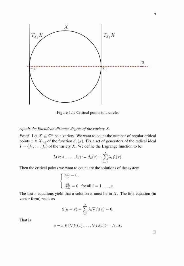
Example 1.0.2 (Circle). Consider X to be a circle in the plane and u a randompoint. Then there are exactly two critical points to the distance function. If u waschosen to be a real point then also the critical points are real. Moreover for everycritical point the data point u lies on the normal line to the circle at the given point.
As we could see from the above example a regular point x P X is critical ifand only if the vector u ´ x is in the normal space at x to X . And indeed in thegeneral setting using Lagrange multipliers, and the observation that the gradientof du is ∇du “ 2pu´ xq, the problem of computing all the regular critical pointsof du amounts to computing all regular points x P X such that the differenceu´ x “ pu1´ x1, . . . , un´ xnq is in the normal space NxX of X at x. We recallthat the normal space is the orthogonal complement of the tangents space at thegiven point to the variety. We make this precise in the next lemma.
Lemma 1.0.3. Given an algebraic variety X Ď Cn and a general data pointu P Cn, the number of solutions to the constrains
x P X, x regular and u´ x P NxX, (1.0.1)
7
ux1
X
Tx1X
x2
Tx2X
Figure 1.1: Critical points to a circle.
equals the Euclidean distance degree of the variety X .
Proof. Let X Ď Cn be a variety. We want to count the number of regular criticalpoints x P Xreg of the function dupxq. Fix a set of generators of the radical idealI “ xf1, . . . , fsy of the variety X . We define the Lagrange function to be
Lpx;λ1, . . . , λsq :“ dupxq `sÿ
i“1
λifipxq.
Then the critical points we want to count are the solutions of the system$
&
%
BLBx “ 0,
BLBλi“ 0, for all i “ 1, . . . , s.
The last s equations yield that a solution x must lie in X . The first equation (invector form) reads as
2pu´ xq `sÿ
i“1
λi∇fipxq “ 0.
That isu´ x P x∇f1pxq, . . . ,∇fspxqy “ NxX.
8 CHAPTER 1. THE EUCLIDEAN DISTANCE DEGREE
In view of this lemma it is clear that we want that the normal space NxX at acritical point x is of the same dimension as the variety X; that is one reason whywe only count critical points that are regular points of the variety.
1.1 Equations defining critical points
An algebraic variety X in Cn of codimension c, can be described either implicitly,by a system of polynomial equations in n variables, or (in some cases) parametri-cally, as the closure of the image of a polynomial map ψ : Cn´c Ñ Cn. In whatfollows we take a variety X with an implicit representation, and we derive thepolynomial equations that characterize the critical points of the squared distancefunction du on X .
Fix a set of generators of the radical ideal I “ xf1, . . . , fsy Ă Crx1, . . . , xns ofthe variety X “ V pIq in Cn. Since the ED degree is additive over the componentsof X , we may assume that X is irreducible and that I is a prime ideal.
The formulation in Lemma 1.0.3 translates into a system of polynomial equa-tions as follows. We write JacxpIq for the s ˆ n Jacobian matrix, whose entry inrow i and column j is the partial derivative Bfipxq{Bxj . The singular locus Xsing
of X is defined by
IXsing “ I `@
cˆ c-minors of JacxpIqD
, (1.1.1)
where c is the codimension of X .We now augment the Jacobian matrix JacxpIq with the row vector u ´ x to
get a pc` 1q ˆ n-matrix. That matrix has rank ď c on the critical points of du onX . From the subvariety of X defined by these rank constraints we must removecontributions from the singular locusXsing. Before the next definition we need thefollowing.
Definition 1.1.1. If I and J are ideals of a ring R, then the the saturation of Iwith respect to J is the ideal defined by
tf P R|Dn P N : Jn ¨ f Ď Iu,
and it is denoted by I : J8.
Definition 1.1.2. The critical ideal for u P Cn is the following saturation:ˆ
I `
B
pc` 1q ˆ pc` 1q-minors ofˆ
u´ xJacxpIq
˙F˙
:`
IXsing
˘8. (1.1.2)
Note that if I were not radical, then the above ideal could have an empty vari-ety.
1.1. EQUATIONS DEFINING CRITICAL POINTS 9
Lemma 1.1.3. For general u P Cn, the variety of the critical ideal in Cn is finite.It consists precisely of the critical points of the squared distance function du onXzXsing.
Proof. For fixed x P XzXsing, the Jacobian JacxpIq has rank c, so the data points
u where the pc`1q ˆ pc`1q-minors ofˆ
u´ xJacxpIq
˙
vanish form an affine-linear
subspace in Cn of dimension c. Hence the variety of pairs px, uq P X ˆ Cn thatare zeros of (1.1.2) is irreducible of dimension n. The fiber of its projection intothe second factor over a general point u P Cn must hence be finite.
Example 1.1.4 (Linear spaces). Every linear space X has ED degree 1. Herethe critical equations (1.0.3) take the form x P X and u ´ x K X . These linearequations have a unique solution u˚. If u and X are real then u˚ is the uniquepoint in X that is closest to u.
Example 1.1.5 (The Eckart-Young Theorem). Fix positive integers r ď n ď m.Let Mďr
nˆm be the variety of n ˆ m-matrices of rank ď r. This determinantalvariety has
EDdegreepMďrnˆmq “
ˆ
n
r
˙
. (1.1.3)
To see this, we consider a general real n ˆ m-matrix M and its singular valuedecomposition
M “ U ¨ diagpσ1, σ2, . . . , σnq ¨ V. (1.1.4)
Here σ1 ě σ2 ě ¨ ¨ ¨ ě σn are the singular values of M , and U and V areorthogonal matrices of format n ˆ n and m ˆ m respectively. According to theEckart-Young Theorem,
M˚ “ U ¨ diagpσ1, . . . , σr, 0, . . . , 0q ¨ V
is the closest rank r matrix to M . More generally, the critical points of dM are
U ¨ diagp0, . . . , 0, σi1 , 0, . . . , 0, σir , 0, . . . , 0q ¨ V
where ti1 ă . . . ă iru runs over all r-element subsets of t1, . . . , nu. This yieldsthe required formula.
Example 1.1.6 (A code to compute ED degree). The following Macaulay2code computes the ED degree of a specific variety (the circle) in R2:
R = QQ[x_0,x_1];f=x_0ˆ2+x_1ˆ2-1;
10 CHAPTER 1. THE EUCLIDEAN DISTANCE DEGREE
u = {1,2};I=ideal(f);c=codim I;Y=matrix{{x_0-u_0, x_1-u_1}};Jac= jacobian gens I;Jbar=Jac|transpose(Y);EX = I + minors(c+1,Jbar);SingX=I+minors(c,Jac);EXreg=saturate(EX,SingX);degree EXreg
In practice many varieties are rational and they are presented by a parametriza-tion ψ : Cn´c Ñ Cn whose coordinates ψi are rational functions in n ´ c un-knowns t “ pt1, . . . , tn´cq. We can use the parametrization directly to computethe ED degree of X . The squared distance function in terms of the parametersequals
Duptq “nÿ
i“1
pψiptq ´ uiq2.
The equations we need to solve are given by n ´ c rational functions in n ´ cunknowns:
BDu
Bt1“ ¨ ¨ ¨ “
BDu
Btn´c“ 0. (1.1.5)
The critical locus in Cn´c is the set of all solutions to (1.1.5) at which theJacobian of ψ has maximal rank. The closure of the image of this set under ψcoincides with the variety of (1.1.2). Hence, if the parametrization ψ is genericallyfinite-to-one of degree k, then the critical locus in Cn´c is finite, by Lemma 1.1.3,and its cardinality equals k ¨ EDdegreepXq.
1.1.1 ED degree of projective varieties
The variety X Ă Cn is an affine cone if for any x P X also λx P X for all λ P C.This means that its generating ideal I is a homogeneous ideal. By a slight abuse ofnotation, we will identify X with the projective variety given by I in Pn´1. Thisway the affine variety is the cone over the projective one.
Definition 1.1.7. The ED degree of the projective variety X Ď Pn´1 is the EDdegree of the corresponding affine cone in Cn.
To take advantage of the homogeneity of the generators of I , and of the geome-try of projective space Pn´1, we replace the critical ideal (1.1.2) with the followingone.
1.1. EQUATIONS DEFINING CRITICAL POINTS 11
Definition 1.1.8. The projective critical ideal for u P Cn is the following satura-tion:
ˆ
I`
B
pc` 2q ˆ pc` 2q-minors of
¨
˝
ux
JacxpIq
˛
‚
F˙
:`
IXsing ¨ xx21`¨ ¨ ¨`x
2ny
˘8.
(1.1.6)Where the singular locus of the affine cone is the cone over the singular locus ofthe projective variety.
The isotropic quadric Q “ tx P Pn´1 : x21 ` ¨ ¨ ¨ ` x2n “ 0u plays a specialrole, as we can see in the next lemma. The following lemma concerns the transitionbetween affine cones and projective varieties.
Lemma 1.1.9. Fix an affine cone X Ă Cn and a data point u P CnzX . Letx P Xzt0u be such that the corresponding point rxs in Pn´1 does not lie in theisotropic quadric Q. Then rxs lies in the projective variety of (1.1.6) if and only ifsome scalar multiple λx of x lies in the affine variety of (1.1.2). In that case, thescalar λ is unique.
Proof. We prove the statement for a dense subset of the variety of 1.1.2 andof 1.1.6. Since both ideals are saturated with respect to IXsing , it suffices to provethis under the assumption that x P XzXsing; the statement for x P Xsing followsbecause both sets are Zariski closed. So we assume that x P XzXsing, hence theJacobian JacxpIq at x has rank c. If u ´ λx lies in the row space of JacxpIq,then the span of u, x, and the rows of JacxpIq has dimension at most c ` 1. Thisproves the if direction. Conversely, suppose that rxs lies in the variety of (1.1.6).First assume that x lies in the row span of JacxpIq. Then x “
ř
λi∇fipxq forsome λi P C. Now recall that if f is a homogeneous polynomial in Rrx1, . . . , xnsof degree d, then x ¨ ∇fpxq “ d fpxq. Since fipxq “ 0 for all i, we find thatx ¨∇fipxq “ 0 for all i, which implies that x ¨ x “ 0, i.e., rxs P Q. This contra-
dicts the hypothesis, so the matrixˆ
xJacxpIq
˙
has rank c ` 1. But then u ´ λx
lies in the row span of JacxpIq for a unique λ P C.
We defined the ED degree of a projective variety in Pn´1 to be the ED degreeof the corresponding affine cone in Cn, moreover given a data point u the criticalpoints to these two objects are in a one-to-one correspondence, given that none ofthe critical points lies in the isotropic quadric. In particular, the role ofQ highlightsthat the computation of ED degree is a metric problem.
12 CHAPTER 1. THE EUCLIDEAN DISTANCE DEGREE
1.2 The ED correspondence
We start with an irreducible affine varietyX Ă Cn of codimension c that is definedover R, with prime ideal I “ xf1, . . . , fsy in Crx1, . . . , xns.
Definition 1.2.1. The ED correspondence EX is the subvariety of CnxˆCnu definedby the ideal (1.1.2) in the polynomial ring Crx1, . . . , xn, u1, . . . , uns.
Here the ui are unknowns that serve as coordinates on the second factor inCnx ˆ Cnu. Geometrically, EX is the topological closure in Cnx ˆ Cnu of the set ofpairs px, uq such that x P Xreg is a critical point of du.
Theorem 1.2.2. The ED correspondence EX of an irreducible variety X Ď Cn ofcodimension c is an irreducible variety of dimension n inside Cnx ˆ Cnu. The firstprojection πx : EX Ñ X Ă Cnx is an affine vector bundle of rank c over Xreg.Over general data points u P Cn, the second projection πu : EX Ñ Cnu has finitefibers π´1u puq of cardinality equal to the ED degree of X .
Proof. The affine vector bundle property follows directly from the system (1.0.3)or, alternatively, from the matrix representation (1.1.2): fixing x P Xreg, the fiberπ´1x pxq equals txu ˆ px ` pTxXqKq, where the second factor is an affine spaceof dimension c varying smoothly with x. Since X is irreducible, so is EX , andits dimension equals pn ´ cq ` c “ n. For dimension reasons, the projection πucannot have positive-dimensional fibers over general data points u, so those fibersare generically finite sets, of cardinality equal to EDdegreepXq.
Corollary 1.2.3. If X is rational, then so is the ED correspondence EX .
Proof. Let ψ : Cn´c Ñ Cn be a rational map that parametrizes X . Its JacobianJacpψq is an n ˆ pn ´ cq-matrix of rational functions in the standard coordinatest1, . . . , tn´c on Cn´c. The columns of Jacpψq span the tangent space of X at thepoint ψptq for general t P Cn´c. The left kernel of Jacpψq is a linear space ofdimension c. Let tβ1ptq, . . . , βcptqu be a basis of the the kernel of the Jacobian. Inparticular, the βj will also be rational functions in the ti. Now the map
Cn´c ˆ Cc Ñ EX , pt, sq Þш
ψptq, ψptq `cÿ
i“1
siβiptq
˙
is a parametrization of EX , which is birational if and only if ψ is birational.
Example 1.2.4 (Parameterizing the ED correspondence of an ellipse). Let Xdenote the ellipse in C2 with equation x21 ` 4x22 “ 4. Given px1, x2q P X ,the pu1, u2q for which px1, x2q is critical are precisely those on the normal line.
1.3. DUALITY 13
This is the line through px1, x2q with direction px1, 4x2q. Consider the rationalparametrization of X given by ψptq “
´
8t1`4t2
, 4t2´1
1`4t2
¯
, t P C. From ψ we con-struct a parametrization ϕ of the surface EX , so that
Cˆ CÑ EX , pt, sq Þш
ψptq,
ˆ
ps` 1q8t
1` 4t2, p4s` 1q
4t2 ´ 1
1` 4t2
˙˙
.
1.3 Duality
In this section we will considerX Ă Cn to be an irreducible affine cone, or, equiv-alently, a projective variety in Pn´1. Such a variety has a dual variety, denoted byY :“ X˚ Ă Cn, which is defined as follows, where the overline indicates theZariski closure:
Y :“
y P Cn | Dx P XzXsing : y K TxX(
. (1.3.1)
The variety Y is an irreducible affine cone, so we can regard it as an irreducibleprojective variety in Pn´1. That projective variety parametrizes hyperplanes tan-gent to X at non-singular points, if one uses the standard bilinear form on Cn toidentify hyperplanes with points in Pn´1.
The main theorem of this section proves that EDdegreepXq “ EDdegreepY q.Moreover, for general data u P Cn, there is a natural bijection between the criticalpoints of du on the cone X and the critical points of du on the cone Y . Beforepresenting the proof of this theorem first we consider an example.
Example 1.3.1 (Determinantal variety). Fix positive integers r ď n ď m. LetMďrnˆm be the variety of nˆm-matrices of rankď r. By [22, Chap. 1, Prop. 4.11]
we have that the dual variety equals pMďrnˆmq
˚ “ Mďn´rnˆm . From Example 1.1.5
we see that EDdegreepMďrnˆmq “ EDdegreepMďn´r
nˆm q. There is a bijection be-tween the critical points of dM onMďr
nˆm and onMďn´rnˆm . To see this, consider the
singular value decomposition (1.1.4). For a subset I “ ti1, . . . , iru of t1, . . . , nu,we set
MI “ U ¨ diagp. . . , σi1 , . . . , σi2 , . . . , σir , . . .q ¨ V,
where the places of σj for j R I have been filled with zeros in the diagonal matrix.Writing Ic for the complementary subset of size n´ r, we have M “MI `MIc .This decomposition is orthogonal in the sense that
xMI ,MIcy “ trpM tIMIcq “ 0.
It follows that, ifM is real, then |M |2 “ |MI |2`|MIc |
2, where |M |2 “ trpM tMq.As I ranges over all r-subsets, MI runs through the critical points of dM on the
14 CHAPTER 1. THE EUCLIDEAN DISTANCE DEGREE
variety Mďrnˆm, and MIc runs through the critical points of dM on the dual variety
Mďn´rnˆm . Since the formula above reads as |M |2 “ |M ´MIc |
2` |M ´MI |2, we
conclude that the proximity of the real critical points reverses under this bijection.For instance, if MI is the real point on Mďr
nˆm closest to M , then MIc is the realpoint on Mďn´r
nˆm furthest from M .
The following theorem shows that the duality seen in Example 1.3.1 holds ingeneral.
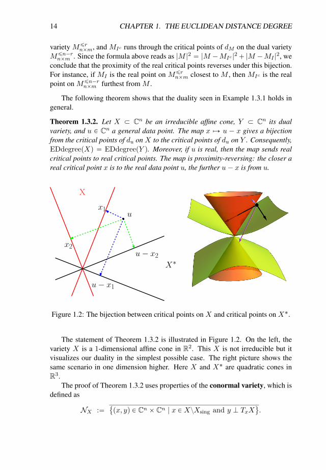
Theorem 1.3.2. Let X Ă Cn be an irreducible affine cone, Y Ă Cn its dualvariety, and u P Cn a general data point. The map x ÞÑ u ´ x gives a bijectionfrom the critical points of du on X to the critical points of du on Y . Consequently,EDdegreepXq “ EDdegreepY q. Moreover, if u is real, then the map sends realcritical points to real critical points. The map is proximity-reversing: the closer areal critical point x is to the real data point u, the further u´ x is from u.
X
X∗
ux1
x2
u− x1
u− x2
Figure 1.2: The bijection between critical points on X and critical points on X˚.
The statement of Theorem 1.3.2 is illustrated in Figure 1.2. On the left, thevariety X is a 1-dimensional affine cone in R2. This X is not irreducible but itvisualizes our duality in the simplest possible case. The right picture shows thesame scenario in one dimension higher. Here X and X˚ are quadratic cones inR3.
The proof of Theorem 1.3.2 uses properties of the conormal variety, which isdefined as
NX :“
px, yq P Cn ˆ Cn | x P XzXsing and y K TxX(
.
1.3. DUALITY 15
It is known that NX is irreducible of dimension n ´ 1. The projection of NXinto the second factor Cn is the dual variety Y “ X˚.
An important property of the conormal variety is the Biduality Theorem ( seefor instance [22, Chapter 1]), which states that NX equals NY up to swapping thetwo factors. So we have
NX “ NY “
px, yq P Cn ˆ Cn | y P Y zYsing and x K TyY(
.
This implies pX˚q˚ “ Y ˚ “ X . Due to this, to keep the symmetry in the notation,from here on we write NX,Y for NX .
Proof of Theorem 1.3.2. The following is illustrated in Figure 1.2. If x is a criticalpoint of du onX , then y :“ u´x is orthogonal to TxX , and hence px, yq P NX,Y .Since u is general, all y thus obtained from critical points x of du are non-singularpoints on Y . By the Biduality Theorem, we have u ´ y “ x K TyY , i.e., y is acritical point of du on Y . This shows that x ÞÑ u ´ x maps critical points of duon X into critical points of du on Y . Applying the same argument to Y , and usingthat Y ˚ “ X , we find that, conversely, y ÞÑ u´ y maps critical points of du on Yto critical points of du on X . This establishes the bijection.
For the last statement we observe that u ´ x K x P TxX for critical x. Fory “ u´ x, this implies
||u´ x||2 ` ||u´ y||2 “ ||u´ x||2 ` ||x||2 “ ||u||2.
Hence the assignments that take real data points u to X and X˚ are proximity-reversing.
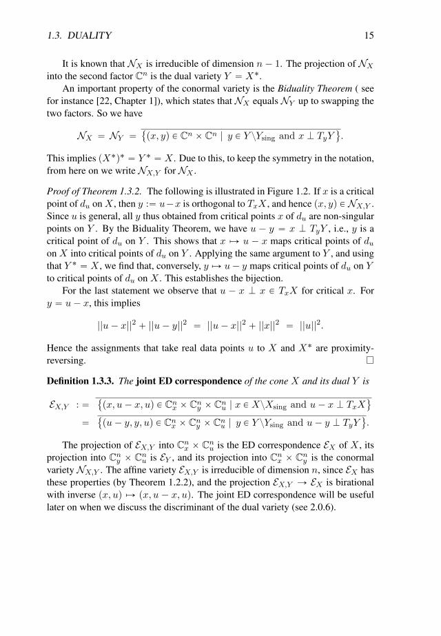
Definition 1.3.3. The joint ED correspondence of the cone X and its dual Y is
EX,Y : “
px, u´ x, uq P Cnx ˆ Cny ˆ Cnu | x P XzXsing and u´ x K TxX(
“
pu´ y, y, uq P Cnx ˆ Cny ˆ Cnu | y P Y zYsing and u´ y K TyY(
.
The projection of EX,Y into Cnx ˆ Cnu is the ED correspondence EX of X , itsprojection into Cny ˆ Cnu is EY , and its projection into Cnx ˆ Cny is the conormalvarietyNX,Y . The affine variety EX,Y is irreducible of dimension n, since EX hasthese properties (by Theorem 1.2.2), and the projection EX,Y Ñ EX is birationalwith inverse px, uq ÞÑ px, u ´ x, uq. The joint ED correspondence will be usefullater on when we discuss the discriminant of the dual variety (see 2.0.6).

16 CHAPTER 1. THE EUCLIDEAN DISTANCE DEGREE

Chapter 2
Discriminants
17
18 CHAPTER 2. DISCRIMINANTS
In the next two chapters we will discuss two different approaches to determine,or at least bound, the number of real critical points of the distance function to analgebraic variety. The first approach is via discriminants. This chapter relies onarticle [27] of the author and parts of the work of Draisma, Horobet, Ottaviani,Sturmfels and Thomas [18].
As can be seen from the definition of the ED degree, the number of complexcritical points is only constant outside a measure zero set. This exceptional set ofdata points where the number of critical points differs from the generic number iscalled the ED-discriminant. For real valued data the number of real critical pointsis constant on the connected components of the complement of the discriminant.
Recall that πu : EX Ñ Cn is the projection from the ED-correspondence tothe data space. Then a more precise definition of the discriminant is as follows.
Definition 2.0.4. The ED-discriminant is the closure of the image of the ramifica-tion locus of πu, i.e., the points where the derivative of πu is not of full rank, underthe projection πu.
This ramification locus is typically an algebraic hypersurface in EX , by theNagata-Zariski Purity Theorem [39],[50].
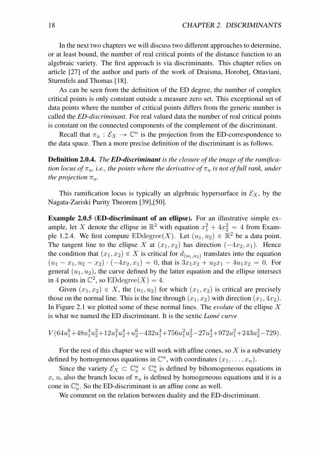
Example 2.0.5 (ED-discriminant of an ellipse). For an illustrative simple ex-ample, let X denote the ellipse in R2 with equation x21 ` 4x22 “ 4 from Exam-ple 1.2.4. We first compute EDdegreepXq. Let pu1, u2q P R2 be a data point.The tangent line to the ellipse X at px1, x2q has direction p´4x2, x1q. Hencethe condition that px1, x2q P X is critical for dpu1,u2q translates into the equationpu1 ´ x1, u2 ´ x2q ¨ p´4x2, x1q “ 0, that is 3x1x2 ` u2x1 ´ 4u1x2 “ 0. Forgeneral pu1, u2q, the curve defined by the latter equation and the ellipse intersectin 4 points in C2, so EDdegreepXq “ 4.
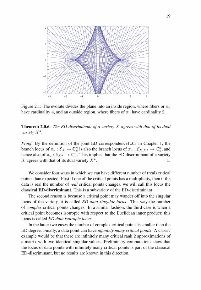
Given px1, x2q P X , the pu1, u2q for which px1, x2q is critical are preciselythose on the normal line. This is the line through px1, x2q with direction px1, 4x2q.In Figure 2.1 we plotted some of these normal lines. The evolute of the ellipse Xis what we named the ED discriminant. It is the sextic Lame curve
V p64u61`48u41u22`12u21u
42`u
62´432u41`756u21u
22´27u42`972u21`243u22´729q.
For the rest of this chapter we will work with affine cones, soX is a subvarietydefined by homogeneous equations in Cn, with coordinates px1, . . . , xnq.
Since the variety EX Ă Cnx ˆ Cnu is defined by bihomogeneous equations inx, u, also the branch locus of πu is defined by homogeneous equations and it is acone in Cnu. So the ED-discriminant is an affine cone as well.
We comment on the relation between duality and the ED-discriminant.
19
-3 -2 -1 0 1 2 3
-2
-1
0
1
2
Figure 2.1: The evolute divides the plane into an inside region, where fibers or πuhave cardinality 4, and an outside region, where fibers of πu have cardinality 2.
Theorem 2.0.6. The ED-discriminant of a variety X agrees with that of its dualvariety X˚.
Proof. By the definition of the joint ED correspondence1.3.3 in Chapter 1, thebranch locus of πu : EX Ñ Cnu is also the branch locus of πu : EX,X˚ Ñ Cnu, andhence also of πu : EX˚ Ñ Cnu. This implies that the ED discriminant of a varietyX agrees with that of its dual variety X˚.
We consider four ways in which we can have different number of (real) criticalpoints than expected. First if one of the critical points has a multiplicity, then if thedata is real the number of real critical points changes, we will call this locus theclassical ED-discriminant. This is a subvariety of the ED-discriminant.
The second reason is because a critical point may wander off into the singularlocus of the variety, it is called ED data singular locus. This way the numberof complex critical points changes. In a similar fashion, the third case is when acritical point becomes isotropic with respect to the Euclidean inner product; thislocus is called ED data isotropic locus.
In the latter two cases the number of complex critical points is smaller than theED degree. Finally, a data point can have infinitely many critical points. A classicexample would be that there are infinitely many critical rank 2 approximations ofa matrix with two identical singular values. Preliminary computations show thatthe locus of data points with infinitely many critical points is part of the classicalED-discriminant, but no results are known in this direction.
20 CHAPTER 2. DISCRIMINANTS
In the following sections we discuss these different subvarieties of the ED-discriminant.
2.1 Classical ED-discriminant
If one of the critical points has a multiplicity, then the number of real criticalpoints changes, we will call this locus the classical ED-discriminant. There is anextensive literature on the classical ED-discriminant (or classically focal locus) seefor instance [49, 18, 22, 30]. We will only recall a couple of these results in thissection. We will denote the classical ED-discriminant of a variety X by ΣX .
Example 2.1.1 (Computing the classical ED-discriminant). This classical ED-discriminant can be computed using the following Macaulay2 code:
n=2;kk=QQ[x_1..x_n,y_1..y_n];f=x_1ˆ2+4*x_2ˆ2-4;I=ideal(f);c=codim I;Y=matrix{{x_1..x_n}}-matrix{{y_1..y_n}};Jac= jacobian gens I;S=submatrix(Jac,{0..n-1},{0..numgens(I)-1});Jbar=S|transpose(Y);EX = I + minors(c+1,Jbar);SingX=I+minors(c,Jac);EXreg=saturate(EX,SingX);Elim=eliminate(toList(x_1..x_(n-1)),EX);M=gens Elim;Disc=discriminant(M_(0,0),x_n);oofactor Disc
It is always interesting to know the degree of the discriminant, for a generalhypersurface the following theorem gives the degree of ΣX .
Theorem 2.1.2 (Trifogli [49]). If X is a general homogeneous hypersurface ofdegree d in Cn then
degreepΣXq “ dpn´ 2qpd´ 1qn´2 ` 2dpd´ 1qpd´ 1qn´2 ´ 1
d´ 2. (2.1.1)
Example 2.1.3 (General plane curve). For a general plane curve X (n “ 3) wehave that degreepΣXq “ 3dpd ´ 1q. And indeed this agrees with our findings forthe ellipse (d “ 2), which had a classical ED-discriminant of degree 6.
2.2. DATA SINGULAR LOCUS 21
Example 2.1.4 (Plane curves). The classical ED-discriminant ΣX of a planecurve X was already studied in the 19th century under the name evolute. Salmon[45, page 96, art. 112] showed that a curve X Ă P2 of degree d with δ ordinarynodes and k ordinary cusps has degreepΣXq “ 3d2 ´ 3d´ 6δ ´ 8k. Curves withmore general singularities are considered in [11, 30] in the context of caustics,which are closely related to evolutes.
Example 2.1.5 (Determinantal variety). Denote by Mďrnˆm the variety of nˆm
matrices (suppose n ď m) of rank at most r. The classical ED-discriminantΣMďr
nˆmdoes not depend on r and equals the discriminant of the characteristic
polynomial of the symmetric matrix UUT , where U is the data matrix. This poly-nomial has been expressed as a sum of squares in [29]. The set of real points in thehypersurface V pΣMďr
nˆmq has codimension two in the space of real nˆmmatrices;
see [46, §7.5]. This explains why the complement of this classical ED-discriminantin the space of real matrices is connected. In particular, if the data matrix U is realthen all critical points are real.
2.2 Data singular locus
When defining the ED degree of a variety, we only allow regular points of thevariety to be called critical points, so we exclude the singular points from ourcomputations. In this manner if one of the critical points wanders off to the singularlocus, then the number of regular critical critical points changes. The study of thespecial locus of data points where this happens was proposed by Bernd Sturmfels,first examples were developed by the authors of [19] and it was named ED datasingular locus. We use the precise definition of the ED data singular locus from[19].
Definition 2.2.1. The ED data singular locus of a variety X is the closure of
πupEX X π´1x pXsingqq.
We denote the ED data singular locus of an algebraic variety X by DSpXq(abbreviating “data singular” ) and we aim to describe the data singular locus ofaffine cones. Our main result in this section is the following theorem.
Theorem 2.2.2. Let X Ď Cn be an irreducible affine cone that is not a linearspace. Then the following two inclusions hold
X˚ Ďp1q DSpXq Ďp2q X˚ `Xsing,
where X˚ denotes the dual variety to X and ` is the Minkowski sum in Cn.
22 CHAPTER 2. DISCRIMINANTS
We view X˚ as subset of Cn via the standard symmetric bilinear form p¨|¨q onCn, see Definition 1.3.1.
Proof. First we prove inclusion p1q for a dense subset ofX˚. For this take u P X˚,such that there exists a regular point xr P Xreg, such that u K TxrX , that is all the
pc` 1q ˆ pc` 1q minors ofˆ
uJacxrpIq
˙
vanish, where c is the codimension of
X and JacxrpIq is the Jacobian of the (radical) ideal I of X at the point xr. We
denote an arbitrary pc` 1q ˆ pc` 1q minor of this matrix byˆ
uJacxrpIq
˙
pc`1q
.
We claim that pu ` λxr, λxrq P EX for all real λ ě 0. We have that if f P I ,homogeneous of degree d, then∇fpλxq “ λd´1∇fpxq. So if xr is a regular pointthen λxr is also regular, for any λ ą 0. Moreover we get that for any pc`1qˆpc`1qminorˆ
pu` λxrq ´ λxrJacλxr
pIq
˙
pc`1q
“
ˆ
uJacλxr
pIq
˙
pc`1q
“ λNˆ
uJacxr
pIq
˙
pc`1q
“ 0,
whereN is the sum of degrees of the defining polynomials of I . So pu`λxr, λxrq P EXfor all real λ ą 0. But then taking the limit when λ goes to zero, we get that
pu, 0q P EX X π´1x pXsingq,
since EX X π´1x pXsingq is Zariski closed (hence closed wrt. Euclidean topologyas well) and since 0 P Xsing. Indeed, for every x P X the line tλ ¨ xu is in thetangent space to 0, so T0X is equal to the the linear span of X , which has a greaterdimension that X if and only if X is not a linear space, hence 0 P Xsing. So thenu “ πxppu, 0qq P DSpXq.
For the proof of p2q take an element pu, x0q P EX X π´1x pXsingq, then thispoint can be approximated by a sequence in the part of EX overXreg. That is thereexists a sequence δi Ñ 0 in Cn and xi Ñ x0 with all the xi P Xreg, such that
pu` δi, xiq P EX .
By the ED Duality Theorem for affine cones 1.3.2 we get that pu` δiq ´ xi P X˚,for all i. Now taking the limit, when i goes to infinity, we get that u ´ x0 P X
˚,since X˚ is closed (hence closed wrt. Euclidean topology as well). Finally thismeans that u P x0 `X˚ Ď Xsing `X
˚.
Note that the condition in the theorem that X is not a linear space is neces-sary. Otherwise if X is a linear subspace of Cn, then it has a non-empty dual (itsorthogonal complement with respect to the inner product), but its singular locus isempty, hence its data singular locus is empty as well.
2.2. DATA SINGULAR LOCUS 23
We want to mention here that a similar theorem holds for the ML (maximumlikelihood) degree, where the data singular locus is defined in a somewhat analo-gous way. The theorem is as follows.
Theorem 2.2.3 (Horobet-Rodriguez [28]). LetX be an algebraic statistical modelin Pn`1. Then, the following two inclusions hold
pXsingzHq ˚ r1 : . . . : 1 : ´1s Ďp1q DSpXq Ďp2q pXsingzHq ˚X˚,
where DSpXq is the data singular locus, X˚ is the dual variety, XsingzH is theopen part of the singular locus where none of the coordinates are zero and theHadamard product ˚ is considered as in [28].
2.2.1 Examples of the ED data singular locus
In this section we present several useful examples concerning the ED data singu-lar locus of an affine cone. Before we get to the examples we present how canone computationally determine the objects we are working with. We illustrate themain algorithms with code in Macaulay2 [23]. For an affine cone X Ď Cn, ofcodimension c with defining radical ideal I , one can determine its dual X˚ usingthe following code by [7, Algorithm 5.1].
Example 2.2.4 (Computing the dual variety). We present the algorithm for thereal affine cone X Ď C3 defined by the homogeneous equation f “ x31 ` x
22x3.
n=3;kk=QQ[x_1..x_n,y_1..y_n];f=x_1ˆ3+x_2ˆ2*x_3;I=ideal(f);c=codim I;Y=matrix{{y_1..y_n}};Jac= jacobian gens I;S=submatrix(Jac,{0..n-1},{0..numgens(I)-1});Jbar=S|transpose(Y);EX = I + minors(c+1,Jbar);SingX=I+minors(c,Jac);EXreg=saturate(EX,SingX);IDual=eliminate(toList(x_1..x_n),EXreg)
Which gives at the end that the dual variety is the zero locus of the polynomialf˚ “ 4x31 ´ 27x22x3.
Following the definition of the data singular locus, the next example containsan algorithm for calculating the ideal of it.
24 CHAPTER 2. DISCRIMINANTS
Example 2.2.5 (Computing the data singular locus). We present the algorithmfor the real affine cone X Ď C3 defined by f “ x31 ` x
22x3.
n=3;kk=QQ[x_1..x_n,y_1..y_n];f=x_1ˆ3+x_2ˆ2*x_3;I=ideal(f);c=codim I;Y=matrix{{x_1..x_n}}-matrix{{y_1..y_n}};Jac= jacobian gens I;S=submatrix(Jac,{0..n-1},{0..numgens(I)-1});Jbar=S|transpose(Y);EX = I + minors(c+1,Jbar);SingX=I+minors(c,Jac);EXreg=saturate(EX,SingX);DSX=radical eliminate(toList(x_1..x_n),EXreg+SingX)
Which gives as output that DSpXq is defined by x1p4x31 ´ 27x22x3q.
Now we arrived at the point to present a sequence of interesting varieties andthe corresponding duals and data singular loci. The first example is the one weused for presenting the algorithms previously. In this example both inclusion p1qand inclusion p2q are strict, as it will be seen.
Example 2.2.6 (Cuspidal Cubic Cone). Let X Ď C3 be the real variety definedby the homogeneous equation f “ x31 ` x22x3. Since it is an affine cone it has adual X˚, which is defined by the dual equation f˚ “ 4x31 ´ 27x22x3. We get thatDSpXq is the zero locus of x1p4x31 ´ 27x22x3q. So we can see that X˚ is even acomponent of DSpXq. Moreover X˚ ` Xsing is a much larger set and not equalto DSpXq. For example the point p3, 2, 1q ` p0, 0, 1q P X˚ `Xsing, but is not onDSpXq. Figure 2.2 shows X in blue and X˚ in green and DSpXq is the union ofthe green colored X˚ and the additional surface in red.
The next example shows that both inclusions p1q and p2q can be in fact equali-ties. More generally we have the following corollary to Theorem 2.2.2.
Corollary 2.2.7. Let X Ď Cn be an affine cone, with Xsing “ t0u, then we havethat DSpXq “ X˚. Moreover if X is a general hypersurface of degree d, then
degpDSpXqq “ dpd´ 1qn´1.
Proof. The first part follows directly from the claim of Theorem 2.2.2. The more-over part is classical and we refer to [7, Exercise 5.14].
2.2. DATA SINGULAR LOCUS 25
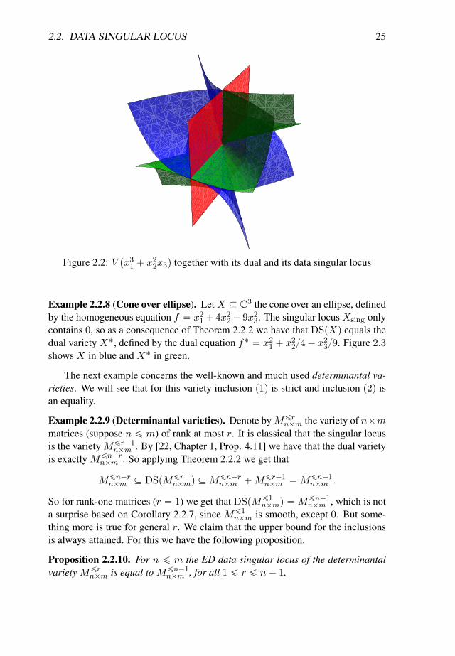
Figure 2.2: V px31 ` x22x3q together with its dual and its data singular locus
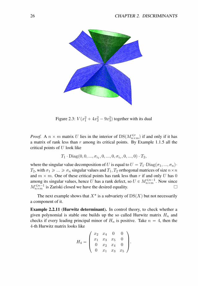
Example 2.2.8 (Cone over ellipse). Let X Ď C3 the cone over an ellipse, definedby the homogeneous equation f “ x21` 4x22´ 9x23. The singular locus Xsing onlycontains 0, so as a consequence of Theorem 2.2.2 we have that DSpXq equals thedual variety X˚, defined by the dual equation f˚ “ x21 ` x
22{4´ x
23{9. Figure 2.3
shows X in blue and X˚ in green.
The next example concerns the well-known and much used determinantal va-rieties. We will see that for this variety inclusion p1q is strict and inclusion p2q isan equality.
Example 2.2.9 (Determinantal varieties). Denote byMďrnˆm the variety of nˆm
matrices (suppose n ď m) of rank at most r. It is classical that the singular locusis the variety Mďr´1
nˆm . By [22, Chapter 1, Prop. 4.11] we have that the dual varietyis exactly Mďn´r
nˆm . So applying Theorem 2.2.2 we get that
Mďn´rnˆm Ď DSpMďr
nˆmq ĎMďn´rnˆm `Mďr´1
nˆm “Mďn´1nˆm .
So for rank-one matrices (r “ 1) we get that DSpMď1nˆmq “Mďn´1
nˆm , which is nota surprise based on Corollary 2.2.7, since Mď1
nˆm is smooth, except 0. But some-thing more is true for general r. We claim that the upper bound for the inclusionsis always attained. For this we have the following proposition.
Proposition 2.2.10. For n ď m the ED data singular locus of the determinantalvariety Mďr
nˆm is equal to Mďn´1nˆm , for all 1 ď r ď n´ 1.
26 CHAPTER 2. DISCRIMINANTS
Figure 2.3: V px21 ` 4x22 ´ 9x23q together with its dual
Proof. A n ˆm matrix U lies in the interior of DSpMďrnˆmq if and only if it has
a matrix of rank less than r among its critical points. By Example 1.1.5 all thecritical points of U look like
T1 ¨Diagp0, 0, ..., σi1 , 0, ..., 0, σir , 0, ..., 0q ¨ T2,
where the singular value decomposition of U is equal to U “ T1 ¨Diagpσ1, ..., σnq¨T2, with σ1 ě ... ě σn singular values and T1, T2 orthogonal matrices of size nˆnand m ˆm. One of these critical points has rank less than r if and only U has 0among its singular values, hence U has a rank defect, so U P Mďn´1
nˆm . Now sinceMďn´1nˆm is Zariski closed we have the desired equality.
The next example shows that X˚ is a subvariety of DSpXq but not necessarilya component of it.
Example 2.2.11 (Hurwitz determinant). In control theory, to check whether agiven polynomial is stable one builds up the so called Hurwitz matrix Hn andchecks if every leading principal minor of Hn is positive. Take n “ 4, then the4-th Hurwitz matrix looks like
H4 “
¨
˚
˚
˝
x2 x4 0 0x1 x3 x5 00 x2 x4 00 x1 x3 x5
˛
‹
‹
‚
.
2.3. DATA ISOTROPIC LOCUS 27
The ratio Γ4 “ detpH4q{x5 is a homogeneous polynomial and it is called theHurwitz determinant for n “ 4 by [18, Example 3.5].
Let X Ď C5 be the affine cone defined by Γ4. Then its dual variety has oneirreducible component given by
X˚ “ V p´x3x4 ` x2x5,´x23 ` x1x5,´x2x3 ` x1x4q.
While its data singular locus DSpXq has two irreducible components and it isdefined by
px1x22`x2x3x4`x
24x5qpx
42x3´x1x
32x4´2x1x2x
34´x3x
44`2x32x4x5`x2x
34x5q.
It is clear that X˚ is not component of DSpXq. Moreover DSpXq is not equal toX˚ `Xsing, since Xsing “ V px2, x4q and the point
p2, 1, 1, 0, 1q “ p1, 1, 0, 0, 0q ` p1, 0, 1, 0, 1q
lies on X˚ `Xsing but it is not on DSpXq.
We have thus seen examples of varieties with: both inclusions in Theorem 2.2.2being strict, both inclusions in Theorem 2.2.2 being equalities and the second in-clusion being an equality, while the first one is strict. It is natural to ask if thereare examples where the first inclusion is an equality, while the second one is strict.The author could not find such an example, so the following question arises.
Problem 2.2.12. Find an affine cone X , such that X˚ “ DSpXq Ă X˚ `Xsing
or prove that there is no such X .
2.3 Data isotropic locus
A next possibility for a data point u to have smaller number of critical points thanexpected is by letting one of the critical points to become isotropic. In Chapter 1we define the ED degree of a projective variety in Pn´1 to be the ED degree of thecorresponding affine cone in Cn, moreover given a data point u the critical pointsto these two objects are in a one-to-one correspondence, given that none of thecritical points lies in the isotropic quadric (see 1.1.9). In particular, the role of Qexhibits that the computation of ED degree is a metric problem. This is the reasonthat even though in the definition of the affine EX we keep the isotropic criticalpoints, when we pass to projective varieties we exclude the isotropic points. Thisway the data isotropic locus represents the locus of data points which have differentnumber of critical points if X is considered as an affine cone or if is considered asa projective variety.
28 CHAPTER 2. DISCRIMINANTS
Definition 2.3.1. The ED data isotropic locus of the variety X is the closure of
πupEX X π´1x pQXXq,
where Q “ V přni“1 x
2i q denotes the isotropic quadric with respect to the standard
symmetric bilinear form.
We denote the ED data isotropic locus of an algebraic variety X by DIpXq(abbreviating “data isotropic”). We have the following theorem for the ED dataisotropic locus of affine cones.
Theorem 2.3.2. Let X Ď Cn be an irreducible affine cone. Then the followingtwo inclusions hold
X˚ Ďp1q DIpXq Ďp2q X˚ ` pQXXq,
where X˚ denotes the dual variety to X .
Again we view X˚ as subset of Cn via the standard symmetric bilinear formp¨|¨q on Cn.
Proof. The proof follows the lines of the proof of 2.2.2, keeping in mind that0 P X is always an isotropic point.
In the following two sections we will give examples to show that both inclu-sions appearing in Theorem 2.2.2 and Theorem 2.3.2 can be strict and/or equalities.
2.3.1 Examples of the ED data isotropic locus
In this section we present several application oriented examples concerning theED data isotropic locus of an affine cone. We begin with presenting how can onecomputationally determine the data isotropic locus of a variety.
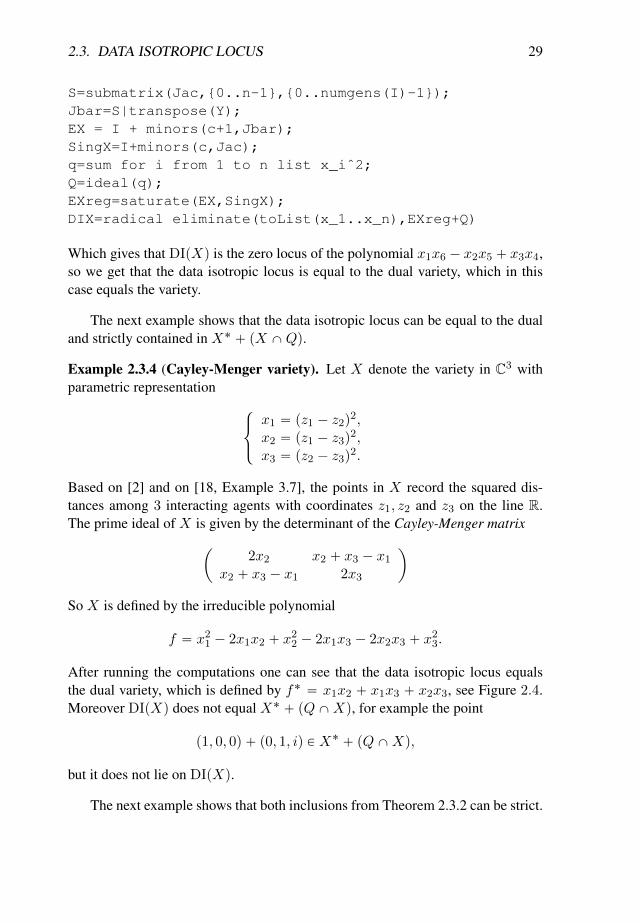
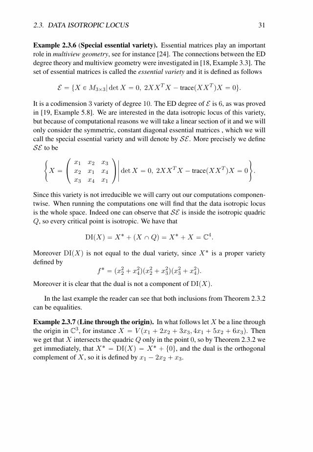
Example 2.3.3 (Computing the data isotropic locus). We present the algorithmfor the real affine cone X Ď C6 defined by f “ x1x6´x2x5`x3x4, representingthe Grassmannian of planes in 4-space.
n=6;kk=QQ[x_1..x_n,y_1..y_n];f=x_1*x_6-x_2*x_5+x_3*x_4;I=ideal(f);c=codim I;Y=matrix{{x_1..x_n}}-matrix{{y_1..y_n}};Jac= jacobian gens I;
2.3. DATA ISOTROPIC LOCUS 29
S=submatrix(Jac,{0..n-1},{0..numgens(I)-1});Jbar=S|transpose(Y);EX = I + minors(c+1,Jbar);SingX=I+minors(c,Jac);q=sum for i from 1 to n list x_iˆ2;Q=ideal(q);EXreg=saturate(EX,SingX);DIX=radical eliminate(toList(x_1..x_n),EXreg+Q)
Which gives that DIpXq is the zero locus of the polynomial x1x6 ´ x2x5 ` x3x4,so we get that the data isotropic locus is equal to the dual variety, which in thiscase equals the variety.
The next example shows that the data isotropic locus can be equal to the dualand strictly contained in X˚ ` pX XQq.
Example 2.3.4 (Cayley-Menger variety). Let X denote the variety in C3 withparametric representation
$
&
%
x1 “ pz1 ´ z2q2,
x2 “ pz1 ´ z3q2,
x3 “ pz2 ´ z3q2.
Based on [2] and on [18, Example 3.7], the points in X record the squared dis-tances among 3 interacting agents with coordinates z1, z2 and z3 on the line R.The prime ideal of X is given by the determinant of the Cayley-Menger matrix
ˆ
2x2 x2 ` x3 ´ x1x2 ` x3 ´ x1 2x3
˙
So X is defined by the irreducible polynomial
f “ x21 ´ 2x1x2 ` x22 ´ 2x1x3 ´ 2x2x3 ` x
23.
After running the computations one can see that the data isotropic locus equalsthe dual variety, which is defined by f˚ “ x1x2 ` x1x3 ` x2x3, see Figure 2.4.Moreover DIpXq does not equal X˚ ` pQXXq, for example the point
p1, 0, 0q ` p0, 1, iq P X˚ ` pQXXq,
but it does not lie on DIpXq.
The next example shows that both inclusions from Theorem 2.3.2 can be strict.
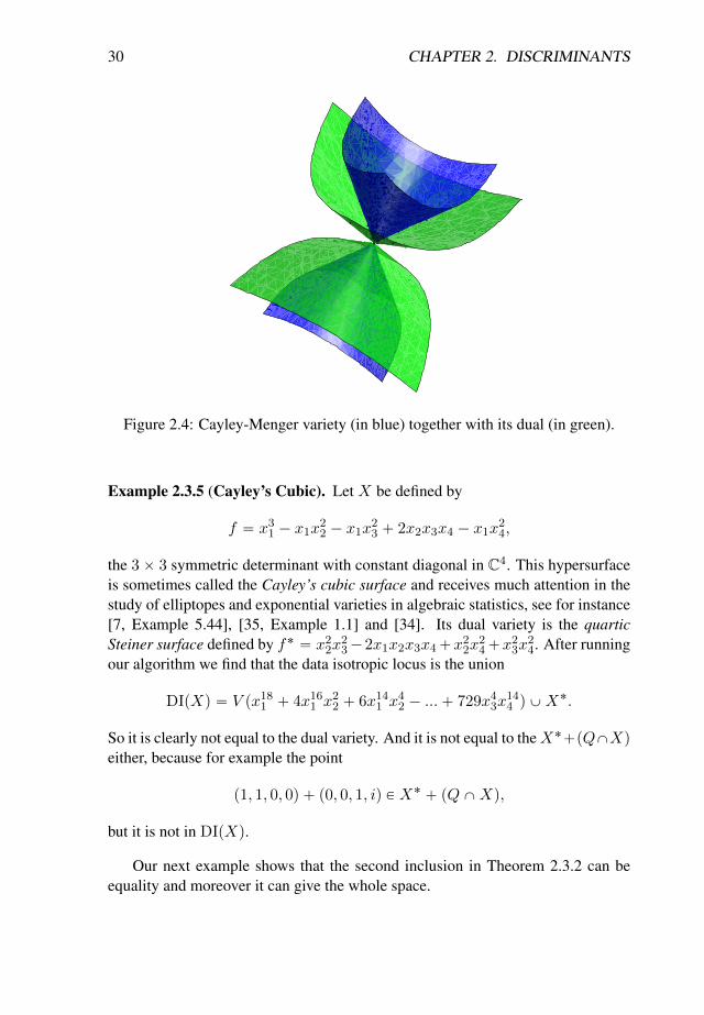
30 CHAPTER 2. DISCRIMINANTS
Figure 2.4: Cayley-Menger variety (in blue) together with its dual (in green).
Example 2.3.5 (Cayley’s Cubic). Let X be defined by
f “ x31 ´ x1x22 ´ x1x
23 ` 2x2x3x4 ´ x1x
24,
the 3ˆ 3 symmetric determinant with constant diagonal in C4. This hypersurfaceis sometimes called the Cayley’s cubic surface and receives much attention in thestudy of elliptopes and exponential varieties in algebraic statistics, see for instance[7, Example 5.44], [35, Example 1.1] and [34]. Its dual variety is the quarticSteiner surface defined by f˚ “ x22x
23´2x1x2x3x4`x
22x
24`x
23x
24. After running
our algorithm we find that the data isotropic locus is the union
DIpXq “ V px181 ` 4x161 x22 ` 6x141 x
42 ´ ...` 729x43x
144 q YX
˚.
So it is clearly not equal to the dual variety. And it is not equal to theX˚`pQXXqeither, because for example the point
p1, 1, 0, 0q ` p0, 0, 1, iq P X˚ ` pQXXq,
but it is not in DIpXq.
Our next example shows that the second inclusion in Theorem 2.3.2 can beequality and moreover it can give the whole space.
2.3. DATA ISOTROPIC LOCUS 31
Example 2.3.6 (Special essential variety). Essential matrices play an importantrole in multiview geometry, see for instance [24]. The connections between the EDdegree theory and multiview geometry were investigated in [18, Example 3.3]. Theset of essential matrices is called the essential variety and it is defined as follows
E “ tX PM3ˆ3| detX “ 0, 2XXTX ´ tracepXXT qX “ 0u.
It is a codimension 3 variety of degree 10. The ED degree of E is 6, as was provedin [19, Example 5.8]. We are interested in the data isotropic locus of this variety,but because of computational reasons we will take a linear section of it and we willonly consider the symmetric, constant diagonal essential matrices , which we willcall the special essential variety and will denote by SE . More precisely we defineSE to be
#
X “
¨
˝
x1 x2 x3x2 x1 x4x3 x4 x1
˛
‚
ˇ
ˇ
ˇ
ˇ
ˇ
detX “ 0, 2XXTX ´ tracepXXT qX “ 0
+
.
Since this variety is not irreducible we will carry out our computations componen-twise. When running the computations one will find that the data isotropic locusis the whole space. Indeed one can observe that SE is inside the isotropic quadricQ, so every critical point is isotropic. We have that
DIpXq “ X˚ ` pX XQq “ X˚ `X “ C4.
Moreover DIpXq is not equal to the dual variety, since X˚ is a proper varietydefined by
f˚ “ px22 ` x24qpx
22 ` x
23qpx
23 ` x
24q.
Moreover it is clear that the dual is not a component of DIpXq.
In the last example the reader can see that both inclusions from Theorem 2.3.2can be equalities.
Example 2.3.7 (Line through the origin). In what follows letX be a line throughthe origin in C3, for instance X “ V px1 ` 2x2 ` 3x3, 4x1 ` 5x2 ` 6x3q. Thenwe get that X intersects the quadric Q only in the point 0, so by Theorem 2.3.2 weget immediately, that X˚ “ DIpXq “ X˚ ` t0u, and the dual is the orthogonalcomplement of X , so it is defined by x1 ´ 2x2 ` x3.

32 CHAPTER 2. DISCRIMINANTS

Chapter 3
Average number of critical points
33
34 CHAPTER 3. AVERAGE NUMBER OF CRITICAL POINTS
In this chapter we will deal with the average ED degree of a real affine varietyX in Rn. In applications, the data point u lies in Rn. The ED degree measures thealgebraic complexity of writing the optimal solution to this approximation problemas a function of the data u. When applying non-algebraic methods for finding theoptimum, the number of real-valued critical points of du for randomly sampleddata u is of high interest. In contrast with the number of complex-valued criticalpoints, this number is typically not constant for all general u, but rather constant onthe connected components of the complement of the ED-discriminant defined inChapter 2. To get a meaningful count of the critical points, we propose to averageover all u with respect to a measure on Rn. This chapter is mainly based on thearticle of Draisma and Horobet[17] and parts of the work of Draisma, Horobet,Ottaviani, Sturmfels and Thomas [18].
3.1 Definitions and introductory examples
In this section we describe how to compute that average using the ED correspon-dence. The presented method is particularly useful when X and hence EX haverational parameterizations.
We impose a probability distribution on our data space Rn with density func-tion ω which satisfies that
ş
Rn |ω| “ 1. A common choice for ω is the standardmultivariate Gaussian 1
p2πqn{2e´||x||
2{2. This choice is natural when X is an affinecone: in that case, the origin 0 is a distinguished point in Rn, and the number ofreal critical points will be invariant under scaling u. Now we ask for the expectednumber of critical points of du when u is drawn from the probability distributionon Rn with density |ω|. Formally we have the following definition.
Definition 3.1.1. The average ED degree of the pair pX,ωq is
aEDdegreepX,ωq :“
ż
Rn#treal critical points of du on Xu ¨ |ω|. (3.1.1)
In the formulas below, we write EX for the set of real points of the ED corre-spondence. Using the substitution rule from multivariate calculus, we rewrite theintegral in (3.1.1) as follows:
aEDdegreepX,ωq “
ż
Rn#π´1u puq ¨ |ω| “
ż
EX|π˚upωq|, (3.1.2)
where π˚upωq is the pull-back of the volume form ω along the derivative of the mapπu. Recall from 1.2.2, that πu is the projection of EX onto the data space Rnu. SeeFigure 3.1 for an illustration of the computation in (3.1.2). Note that π˚upωq neednot be a volume form since it vanishes at the inverse image of the ED-discriminant.
3.1. DEFINITIONS AND INTRODUCTORY EXAMPLES 35
Rn
EX
πu
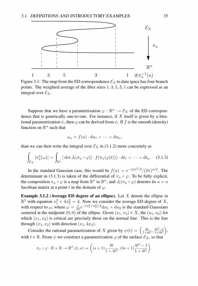
#π−1u (u)1 3 5 3 1
Figure 3.1: The map from the ED correspondence EX to data space has four branchpoints. The weighted average of the fiber sizes 1, 3, 5, 3, 1 can be expressed as anintegral over EX .
Suppose that we have a parametrization ϕ : Rn Ñ EX of the ED correspon-dence that is generically one-to-one. For instance, if X itself is given by a bira-tional parametrization ψ, thenϕ can be derived from ψ. If f is the smooth (density)function on Rn such that
ωu “ fpuq ¨ du1 ^ ¨ ¨ ¨ ^ dun,
than we can then write the integral over EX in (3.1.2) more concretely asż
EX|π˚upωq| “
ż
Rn| det Jtpπu ˝ ϕq| ¨ fpπupϕptqqq ¨ dt1 ^ ¨ ¨ ¨ ^ dtn. (3.1.3)
In the standard Gaussian case, this would be fpuq “ e´||u||2{2{p2πqn{2. The
determinant in (3.1.3) is taken of the differential of πu ˝ ϕ. To be fully explicit,the composition πu ˝ ϕ is a map from Rn to Rn, and Jtpπu ˝ ϕq denotes its nˆ nJacobian matrix at a point t in the domain of ϕ.
Example 3.1.2 (Average ED degree of an ellipse). Let X denote the ellipse inR2 with equation x21 ` 4x22 “ 4. Now we consider the average ED degree of X ,with respect to ω, where ω “ 1
2πe´pu21`u
22q{2du1 ^ du2 is the standard Gaussians
centered at the midpoint p0, 0q of the ellipse. Given px1, x2q P X , the pu1, u2q forwhich px1, x2q is critical are precisely those on the normal line. This is the linethrough px1, x2q with direction px1, 4x2q.
Consider the rational parametrization of X given by ψptq “´
8t1`4t2
, 4t2´1
1`4t2
¯
,with t P R. From ψ we construct a parametrization ϕ of the surface EX , so that
πu ˝ ϕ : Rˆ RÑ R2, pt, sq ÞÑ
ˆ
ps` 1q8t
1` 4t2, p4s` 1q
4t2 ´ 1
1` 4t2
˙
.
36 CHAPTER 3. AVERAGE NUMBER OF CRITICAL POINTS
The Jacobian determinant of πu ˝ ϕ equals
´32p1` s` 4p2s´ 1qt2 ` 16p1` sqt4q
p1` 4t2q3,
so the average ED degree of X is
1
2π
ż 8
´8
ˆż 8
´8
ˇ
ˇ
ˇ
ˇ
´32p1` s` 4p2s´1qt2 ` 16p1`sqt4q
p1` 4t2q3
ˇ
ˇ
ˇ
ˇ
efpt,sqdt
˙
ds,
wherefpt, sq “
´p1` 4sq2 ´ 8p7´ 8p´1` sqsqt2 ´ 16p1` 4sq2t4
2p1` 4t2q2.
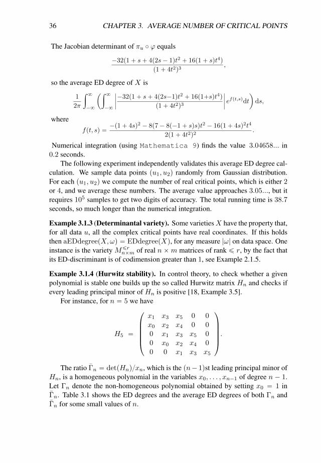
Numerical integration (using Mathematica 9) finds the value 3.04658... in0.2 seconds.
The following experiment independently validates this average ED degree cal-culation. We sample data points pu1, u2q randomly from Gaussian distribution.For each pu1, u2q we compute the number of real critical points, which is either 2or 4, and we average these numbers. The average value approaches 3.05..., but itrequires 105 samples to get two digits of accuracy. The total running time is 38.7seconds, so much longer than the numerical integration.
Example 3.1.3 (Determinantal variety). Some varietiesX have the property that,for all data u, all the complex critical points have real coordinates. If this holdsthen aEDdegreepX,ωq “ EDdegreepXq, for any measure |ω| on data space. Oneinstance is the variety Mďr
nˆm of real nˆm matrices of rank ď r, by the fact thatits ED-discriminant is of codimension greater than 1, see Example 2.1.5.
Example 3.1.4 (Hurwitz stability). In control theory, to check whether a givenpolynomial is stable one builds up the so called Hurwitz matrix Hn and checks ifevery leading principal minor of Hn is positive [18, Example 3.5].
For instance, for n “ 5 we have
H5 “
¨
˚
˚
˚
˚
˝
x1 x3 x5 0 0x0 x2 x4 0 00 x1 x3 x5 00 x0 x2 x4 00 0 x1 x3 x5
˛
‹
‹
‹
‹
‚
.
The ratio Γn “ detpHnq{xn, which is the pn´ 1qst leading principal minor ofHn, is a homogeneous polynomial in the variables x0, . . . , xn´1 of degree n ´ 1.Let Γn denote the non-homogeneous polynomial obtained by setting x0 “ 1 inΓn. Table 3.1 shows the ED degrees and the average ED degrees of both Γn andΓn for some small values of n.
3.2. RANK ONE TENSOR APPROXIMATIONS 37
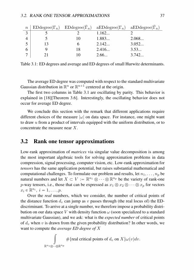
n EDdegreepΓnq EDdegreepΓnq aEDdegreepΓnq aEDdegreepΓnq
3 5 2 1.162... 24 5 10 1.883... 2.068...5 13 6 2.142... 3.052...6 9 18 2.416... 3.53...7 21 10 2.66... 3.742...
Table 3.1: ED degrees and average and ED degrees of small Hurwitz determinants.
The average ED degree was computed with respect to the standard multivariateGaussian distribution in Rn or Rn`1 centered at the origin.
The first two columns in Table 3.1 are oscillating by parity. This behavior isexplained in [18][Theorem 3.6]. Interestingly, the oscillating behavior does notoccur for average ED degree.
We conclude this section with the remark that different applications requiredifferent choices of the measure |ω| on data space. For instance, one might wantto draw u from a product of intervals equipped with the uniform distribution, or toconcentrate the measure near X .
3.2 Rank one tensor approximations
Low-rank approximation of matrices via singular value decomposition is amongthe most important algebraic tools for solving approximation problems in datacompression, signal processing, computer vision, etc. Low-rank approximation fortensors has the same application potential, but raises substantial mathematical andcomputational challenges. To formulate our problem and results, let n1, . . . , np benatural numbers and let X Ă V :“ Rn1 b ¨ ¨ ¨ b Rnp be the variety of rank-onep-way tensors, i.e., those that can be expressed as x1 b x2 b ¨ ¨ ¨ b xp for vectorsxi P Rni , i “ 1, . . . , p.
Over the real numbers, which we consider, the number of critical points ofthe distance function dv can jump as v passes through (the real locus of) the ED-discriminant. To arrive at a single number, we therefore impose a probability distri-bution on our data space V with density function ω (soon specialized to a standardmultivariate Gaussian), and we ask: what is the expected number of critical pointsof dv when v is drawn from the given probability distribution? In other words, wewant to compute the average ED degree of X
ż
Rn1b¨¨¨bRnp
#treal critical points of dv on Xuωpvqdv.
38 CHAPTER 3. AVERAGE NUMBER OF CRITICAL POINTS
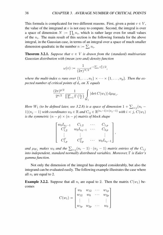
This formula is complicated for two different reasons. First, given a point v P V ,the value of the integrand at v is not easy to compute. Second, the integral is overa space of dimension N :“
ś
i ni, which is rather large even for small valuesof the ni. The main result of this section is the following formula for the aboveintegral, in the Gaussian case, in terms of an integral over a space of much smallerdimension quadratic in the number n :“
ř
i ni.
Theorem 3.2.1. Suppose that v P V is drawn from the (standard) multivariateGaussian distribution with (mean zero and) density function
ωpvq :“1
p2πqN{2e´p
ř
α v2αq{2,
where the multi-index α runs over t1, . . . , n1u ˆ ¨ ¨ ¨ ˆ t1, . . . , npu. Then the ex-pected number of critical points of dv on X equals
p2πqp{2
2n{21
śpi“1 Γ
`
ni2
˘
ż
W1
|detCpw1q|dµW1 .
Here W1 (to be defined later, see 3.2.8) is a space of dimension 1 `ř
iăjpni ´
1qpnj ´ 1q with coordinates w0 P R and Cij P Rpni´1qˆpnj´1q with i ă j, Cpw1q
is the symmetric pn´ pq ˆ pn´ pq matrix of block shape»
—
—
—
–
w0In1´1 C1,2 ¨ ¨ ¨ C1,p
CT1,2 w0In2´1 ¨ ¨ ¨ C2,p...
......
CT1,p CT2,p ¨ ¨ ¨ w0Inp´1
fi
ffi
ffi
ffi
fl
,
and µW1 makes w0 and theř
iăjpni ´ 1q ¨ pnj ´ 1q matrix entries of the Ci,jinto independent, standard normally distributed variables. Moreover, Γ is Euler’sgamma function.
Not only the dimension of the integral has dropped considerably, but also theintegrand can be evaluated easily. The following example illustrates the case whereall ni are equal to 2.
Example 3.2.2. Suppose that all ni are equal to 2. Then the matrix Cpw1q be-comes
Cpw1q “
»
—
—
—
–
w0 w12 ¨ ¨ ¨ w1p
w12 w0 ¨ ¨ ¨ w2p...
......
w1p w2p ¨ ¨ ¨ w0
fi
ffi
ffi
ffi
fl
3.2. RANK ONE TENSOR APPROXIMATIONS 39
where the distinct entries are independent scalar variables „ N p0, 1q. The ex-pected number of critical points of dv on X equals
p2πqp{2
22p{21
Γp11qpEp|detpCpw1qq|q “
´π
2
¯p{2Ep|detpCpw1qq|q,
where the latter factor is the expected absolute value of the determinant of Cpw1q.For p “ 2 that expected value of |w2
0 ´ w212| can be computed symbolically and
equals 4{π. Thus the expression above then reduces to 2, which is just the numberof singular values of a 2 ˆ 2-matrix. For higher p we do not know a closed formexpression for Ep|detpCpw1qq|q, but we will present some numerical approxima-tions in 3.2.3. ♦
In subsection 3.2.1 we prove Theorem 3.2.1, and in subsection 3.2.3 we listsome numerically computed values. These values lead to the following intriguingstabilization conjecture.
Conjecture 3.2.3. Suppose that np ´ 1 ąřp´1i“1 ni ´ 1. Then, in the Gaussian
setting of Theorem 3.2.1, the expected number of critical points of dv on X doesnot decrease if we replace np by np ´ 1.
For p “ 2 this follows from the statement that the number of singular valuesof a sufficiently general n1 ˆ n2-matrix with n1 ă n2 equals n1, which in factremains the same when replacing n2 by n2 ´ 1. For arbitrary p the statement istrue over C as shown in [21], again with equality, but the proof is not bijective.Instead, it uses vector bundles and Chern classes, techniques that do not carry overto our setting. It would be very interesting to find a direct geometric argument thatdoes explain our experimental findings over the reals, as well.
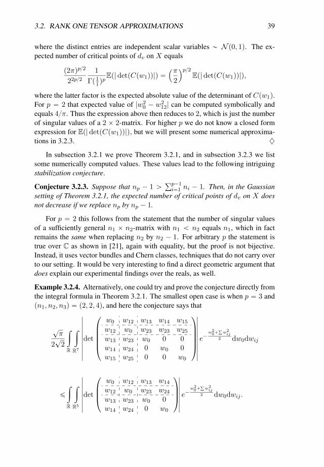
Example 3.2.4. Alternatively, one could try and prove the conjecture directly fromthe integral formula in Theorem 3.2.1. The smallest open case is when p “ 3 andpn1, n2, n3q “ p2, 2, 4q, and here the conjecture says that
?π
2?
2
ż
R
ż
R7
ˇ
ˇ
ˇ
ˇ
ˇ
ˇ
ˇ
ˇ
ˇ
ˇ
det
¨
˚
˚
˚
˚
˝
w0 w12 w13 w14 w15
w12 w0 w23 w23 w25
w13 w23 w0 0 0w14 w24 0 w0 0w15 w25 0 0 w0
˛
‹
‹
‹
‹
‚
ˇ
ˇ
ˇ
ˇ
ˇ
ˇ
ˇ
ˇ
ˇ
ˇ
e´w20`
ř
w2ij
2 dw0dwij
ď
ż
R
ż
R5
ˇ
ˇ
ˇ
ˇ
ˇ
ˇ
ˇ
ˇ
det
¨
˚
˚
˝
w0 w12 w13 w14
w12 w0 w23 w24
w13 w23 w0 0w14 w24 0 w0
˛
‹
‹
‚
ˇ
ˇ
ˇ
ˇ
ˇ
ˇ
ˇ
ˇ
e´w20`
ř
w2ij
2 dw0dwij .
40 CHAPTER 3. AVERAGE NUMBER OF CRITICAL POINTS
The determinant in the first integral is approximately w0 times a determinant likein the second integral, but we do not know how to turn this observation into a proofof this integral inequality. ♦
Symmetric tensors
In the second part of this section, we discuss symmetric tensors. There we considerthe space V “ SpRn of homogeneous polynomials of degree p in the standardbasis e1, . . . , en of Rn, and X is the subvariety of V consisting of all polynomialsthat are of the form ˘up with u P Rn. We equip V with the Bombieri norm(see [3]), in which the monomials in the ei form an orthogonal basis with squarednorms
||eα11 ¨ ¨ ¨ eαnn ||
2 “α1! ¨ ¨ ¨αn!
p!.
Our result on the average number of critical points of dv on X is as follows.
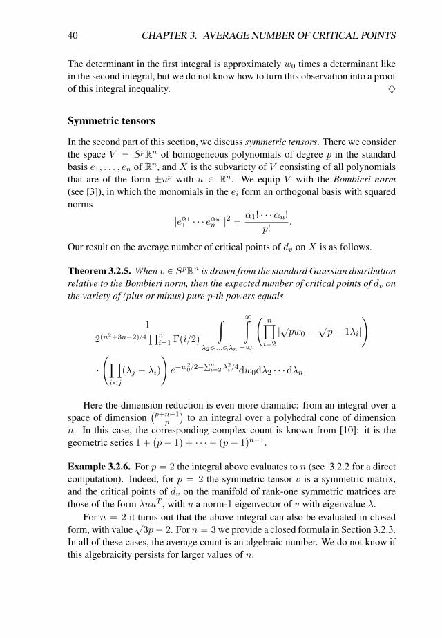
Theorem 3.2.5. When v P SpRn is drawn from the standard Gaussian distributionrelative to the Bombieri norm, then the expected number of critical points of dv onthe variety of (plus or minus) pure p-th powers equals
1
2pn2`3n´2q{4śni“1 Γpi{2q
ż
λ2ď...ďλn
8ż
´8
˜
nź
i“2
|?pw0 ´
a
p´ 1λi|
¸
¨
˜
ź
iăj
pλj ´ λiq
¸
e´w20{2´
řni“2 λ
2i {4dw0dλ2 ¨ ¨ ¨ dλn.
Here the dimension reduction is even more dramatic: from an integral over aspace of dimension
`
p`n´1p
˘
to an integral over a polyhedral cone of dimensionn. In this case, the corresponding complex count is known from [10]: it is thegeometric series 1` pp´ 1q ` ¨ ¨ ¨ ` pp´ 1qn´1.
Example 3.2.6. For p “ 2 the integral above evaluates to n (see 3.2.2 for a directcomputation). Indeed, for p “ 2 the symmetric tensor v is a symmetric matrix,and the critical points of dv on the manifold of rank-one symmetric matrices arethose of the form λuuT , with u a norm-1 eigenvector of v with eigenvalue λ.
For n “ 2 it turns out that the above integral can also be evaluated in closedform, with value
?3p´ 2. For n “ 3 we provide a closed formula in Section 3.2.3.
In all of these cases, the average count is an algebraic number. We do not know ifthis algebraicity persists for larger values of n.
3.2. RANK ONE TENSOR APPROXIMATIONS 41
3.2.1 Ordinary tensors
Suppose that we have equipped V “ RN with an inner product p.|.q and that wehave a smooth manifold X Ď V . Assume that we have a probability density ω onV “ RN and that we want to count the average number of critical points x P X ofdvpxq when v is drawn according to that density. Let EX be the ED-correspence
EX :“ tpv, xq | v ´ x K TxXu Ď V ˆX
of pairs pv, xq P X ˆ V for which x is a critical point of dv. Recall that for fixedx P X the v P V with pv, xq P EX form an affine space, namely, x ` pTxXqK;the normal space translated by the vector x. In particular, EX is a manifold ofdimension N , see 1.2.2.
We apply the method from Section 3.1. Let πV : EX Ñ V be the first projec-tion. Then (the absolute value of) the pull-back |π˚V ωdv| is a pseudo volume formon EX , and we have
ż
V#pπ´1V pvqqωpvqdv “
ż
EX1|π˚V ωdv|.
Now suppose that we have a smooth 1 : 1 parameterization ϕ : RN Ñ EX (definedoutside the inverse image of the ED-discriminant). Then the latter integral is just
ż
RN| det JwpπV ˝ ϕq|ωpπV pϕpwqqqdw,
where JwpπV ˝ ϕq is the Jacobian of πV ˝ ϕ at the point w. We will see that if Xis the manifold of rank-one tensors or rank-one symmetric tensors, then EX (or infact, a slight variant of it) has a particularly friendly parameterization, and we willuse the latter expression to compute the expected number of critical points of dv.
Parameterizing EXTo apply the methods from the previous section 3.1, we introduce a convenientparameterization of EX . Fix norm-1 vectors ei P Vi, i “ 1, . . . , p and writee “ pe1, . . . , epq, res :“ pre1s, . . . , repsq, and define
W :“Wres “
˜
pà
i“1
e1 b ¨ ¨ ¨ b xeiyK b ¨ ¨ ¨ b ep
¸K
.
We parameterize (an open subset of) PVi by the map
xeiyK Ñ PVi, ui ÞÑ rei ` uis.
42 CHAPTER 3. AVERAGE NUMBER OF CRITICAL POINTS
Write U :“śpi“1pxeiy
Kq. For u “ pu1, . . . , upq P U let Ru denote a linearisomorphism W ÑWre`us, to be chosen later, but at least smoothly varying withu and perhaps defined outside some subvariety of positive codimension.
Next defineϕ : W ˆ U Ñ V, pw,uq ÞÑ Ruw.
Then we have the following fundamental identity
1
p2πqN{2
ż
V
p#π´1V pvqq ¨ e
´||v||2
2 dv “1
p2πqN{2
ż
WˆU
|det Jpw,uqϕ|e´||Ruw||2
2 du dw,
where Jpw,uqϕ is the Jacobian of ϕ at pw,uq, whose determinant is measured rela-tive to the volume form on V coming from the inner product and the volume formon W ˆ U coming from the inner products of the factors, which are interpretedperpendicular to each other. The left-hand side is our desired quantity, and ourgoal is to show that the right-hand side reduces to the formula in Theorem 3.2.1.
We choose Ru to be the tensor product Ru1 b ¨ ¨ ¨ b Rup , where Rui is theelement of SOpViq determined by the conditions that it maps ei to a positive scalarmultiple of ei ` ui and that it restricts to the identity on xei, uiyK; this map isunique for non-zero ui P xeiyK. Indeed, we have
Rui“
ˆ
I ´ eieTi ´
ui||ui||
uTi||ui||
˙
`
˜
ei ` uia
1` ||ui||2eTi `
ui ´ ||ui||2ei
||ui||a
1` ||ui||2uTi||ui||
¸
“
ˆ
I ´ eieTi ´
uiuTi
||ui||2
˙
`
˜
ei ` uia
1` ||ui||2eTi `
ui ´ ||ui||2ei
a
1` ||ui||2uTi||ui||2
¸
where the first term is the orthogonal projection to xei, uiyK and the second termis projection onto the plane xei, uiy followed by a suitable rotation there. Twoimportant remarks concerning symmetries are in order. First, by construction ofRui we have
R´1ui “ R´ui . (3.2.1)
Second, for any element g P SOpxeiyKq, considered as an element of the stabilizer
of ei in SOpViq, we have
Rgui “ g ˝Rui ˝ g´1. (3.2.2)
We now compute the derivative at ui of the map xeiyK Ñ SOpViq, u ÞÑ Ru inthe direction vi P xeiyK. First, when vi is perpendicular to both ei and ui, thisderivative equals
BRuiBvi
“1
a
1` ||ui||2pvie
Ti ´eiv
Ti q´
a
1` ||ui||2 ´ 1
||ui||2a
1` ||ui||2puiv
Ti `viu
Ti q. (3.2.3)
3.2. RANK ONE TENSOR APPROXIMATIONS 43
Second, when vi equals ui, the derivative equals
BRuiBui
“1
p1` ||ui||2q3{2p´uiu
Ti ` uie
Ti ´ eiu
Ti ´ ||ui||
2eieTi q. (3.2.4)
For now, fix pw,uq P W ˆ U . On the subspace TwW “ W of Tpw,uqW ˆ U theJacobian of ϕ is just the mapW Ñ V,w ÞÑ Ruw. Hence relative to the orthogonaldecompositions V “WK ‘W and U ˆW , we have a block decomposition
R´1u Jpw,uqϕ “
„
Apw,uq 0
˚ IW
for a suitable matrix Apw,uq. Note that this matrix has size pn ´ pq ˆ pn ´ pq,which is the size of the determinant in Theorem 3.2.1. As Ru is orthogonal withdeterminant 1, we have det Jpw,uqϕ “ detApw,uq and ||Ruw|| “ ||w||. This yieldsthe following proposition.
Proposition 3.2.7. The expected number of critical rank-one approximations to astandard Gaussian tensor in V is
I :“1
p2πqN{2
ż
W
ż
U| detApw,uq|e
´||w||2
2 du dw.
For later use, consider the function F : U Ñ R defined as
F puq “1
p2πqN{2
ż
W| detApw,uq|e
´||w||2
2 dw.
From (3.2.2) and the fact that the Gaussian density onW is orthogonally invariant,it follows that F is invariant under the group
śpi“1 SOpxeiy
Kq. In particular, itsvalue depends only on the tuple p||u1||, . . . , ||up||q “: pt1, . . . , tpq. This will beused in the following part.
The shape of Apw,uq
Recall that U “śpi“1pxeiy
Kq. Correspondingly, the columns of the matrix Apw,uqcome in p blocks, one for each xeiyK. The i-th block records the WK-componentsof the vectors
´
R´1uBRuBvi
¯
w, where vi “ p0, . . . , vi, . . . , 0q and vi runs through an
orthonormal basis ep1qi , . . . , epni´1qi of xeiyK. We have
R´1u
BRu
Bvi“ Idb ¨ ¨ ¨ bR´1ui
BRuiBvi
b ¨ ¨ ¨ b Id. (3.2.5)
44 CHAPTER 3. AVERAGE NUMBER OF CRITICAL POINTS
Furthermore, if vi is also perpendicular to ui, then by 3.2.3 and 3.2.1
R´1uiBRuiBvi
“1
a
1` ||ui||2pvie
Ti ´ eiv
Ti q `
1´a
1` ||ui||2
||ui||2a
1` ||ui||2pviu
Ti ´ uiv
Ti q.
(3.2.6)On the other hand, when vi is parallel to ui, then
R´1uiBRuiBvi
“1
1` ||ui||2pvie
Ti ´ eiv
Ti q. (3.2.7)
This is derived from (3.2.1) and (3.2.4), keeping in mind the fact that here vi needsnot be equal to ui, but merely parallel to it. Note that both matrices are skew-symmetric. This is no coincidence: the directional derivative BRui{Bvi lies in thetangent space to SOpViq at ui, and left multiplying by R´1ui maps these elementsinto the Lie algebra of SOpViq, which consists of skew symmetric matrices.
We decompose the space W as
W “
˜
pà
i“1
e1 b ¨ ¨ ¨ b xeiyK b ¨ ¨ ¨ b ep
¸K
“ R ¨ e1 b e2 b ¨ ¨ ¨ b ep
‘
˜
à
1ďiăjďp
e1 b ¨ ¨ ¨ b xeiyK b ¨ ¨ ¨ b xejy
K b ¨ ¨ ¨ b ep
¸
‘W 1 “: W0 ‘W1,
where W 1 contains the summands that contain at least three xeiyK-s as factors.From (3.2.5) it follows that R´1u
BRuBvi
W 1 Ď W . So for a general w we use theparameters
w “w0 ¨ e1 b ¨ ¨ ¨ b ep
`ÿ
1ďiăjďp
ÿ
1ďaďni´1
ÿ
1ďbďnj´1
wa,bi,j e1 b ¨ ¨ ¨ b epaqi b ¨ ¨ ¨ b e
pbqj b ¨ ¨ ¨ b ep ` w
1,
where w0 and wa,bi,j are real numbers, and where w1 P W 1 will not contribute toApw,uq. We also write
w1 :“ pw0, pwa,bi,j qq, (3.2.8)
for the components of w that do contribute.As a further simplification, we take each ui equal to a scalar ti ě 0 times
the first basis vector ep1qi of xeiyK. This is justified by the observation that thefunction F is invariant under the group
ś
i SOpxeiyKq. Thus we want to determine
A´
w,pt1ep1q1 ,t2e
p1q2 ,...,tpe
p1qp q
¯. This matrix has a natural block structure pBi,jq1ďi,jďp,
where Bi,j is the part of the Jacobian containing the e1 b ¨ ¨ ¨ b xeiyK b ¨ ¨ ¨ b ep-
coordinates of´
R´1uBRuBvj
¯
w with vj “ p0, . . . , vj , . . . , 0q.
3.2. RANK ONE TENSOR APPROXIMATIONS 45
Fixing i ă j, the matrix Bi,j is of type pni´ 1qˆ pnj ´ 1q, where the pa, bq-thelement is the e1 b ¨ ¨ ¨ b e
paqi b ¨ ¨ ¨ b ep-coordinate of
˜
R´1ujBRuj
Bepbqj
¸
w.
First, if b ‰ 1, then we have a directional derivative in a direction perpendicular touj “ tje
p1qj . Applying formula 3.2.6 for the directions epbqj yields
Bi,jpa, bq “´wa,bi,jb
1` t2j
.
Second, if b “ 1, then we consider directional derivatives parallel to uj , so apply-ing formula 3.2.7 for direction ep1qj , we get
Bi,jpa, 1q “´wa,1i,j1` t2j
.
Putting all together, the matrix Bi,j is as follows
Bi,j “
¨
˝
1
1` t2jC1i,j ,
1b
1` t2j
C2i,j , . . . ,
1b
1` t2j
Cnj´1i,j
˛
‚,
where Cbi,j “´
´wa,bi,j
¯
1ďaďni´1are column vectors for all 1 ď b ď nj ´ 1.
Denote the matrix consisting of these column vectors by Ci,j . Doing the samecalculations but now for the matrix Bj,i, and writing Cj,i “ CTi,j , we find that
Bj,i “
¨
˝
1
1` t2iC1j,i,
1b
1` t2i
C2j,i, . . . ,
1b
1` t2i
Cni´1j,i
˛
‚.
The only remaining case is when i “ j, and then similar calculations yield thatBj,j “
1
p1`t2j qnj2
w0Inj´1. We summarize the content of this part as follows.
Proposition 3.2.8. For pw,uq PW ˆ U with u “ pt1ep1q1 , . . . , tpe
p1qp q we have
detApw,uq “
pź
k“1
1
p1` t2kqnk2
det
¨
˚
˚
˚
˝
C1 C1,2 ¨ ¨ ¨ C1,p
CT1,2 C2 ¨ ¨ ¨ C2,p...
......
CT1,p CT2,p ¨ ¨ ¨ Cp
˛
‹
‹
‹
‚
,
where Ci,j “´
´wa,bi,j
¯
a,band Cj “ w0Inj´1 for all 1 ď i ă j ď p.
46 CHAPTER 3. AVERAGE NUMBER OF CRITICAL POINTS
For further reference we denote the above matrix pCi,jq1ďi,jďp by Cpw1q.
The value of I
We are now in a position to prove our formula for the expected number of criticalrank-one approximations to a Gaussian tensor v.
Proof of Theorem 3.2.1. Combine Propositions 3.2.7 and 3.2.8 into the expression
I “1
p2πqN2
pź
k“1
VolpSnk´2q
ż
W
8ż
0
¨ ¨ ¨
8ż
0
pź
i“1
tni´2i
p1` t2i qni2
|detCpw1q| e´||w||2
2 dt1 ¨ ¨ ¨ dtpdw.
Here the factors tni´2i and the volumes of the sphere account for the fact that Fis orthogonally invariant and dui “ tni´2i dtdS , where dS is the surface element ofthe pni ´ 2q-dimensional unit sphere in xeiyK. Now recall that
8ż
0
tni´2
p1` t2qni2
dt “
?π
2
Γpni´12 q
Γpni2 q,
and that the volume of the pn´ 2q-sphere is
VolpSni´2q “2π
ni´1
2
Γpni´12 q.
Plugging in the above two formulas, we obtain
I “
?πn
?2π
N
1śpi“1 Γ
`
ni2
˘
ż
W
|detCpwq| e´||w||2
2 dw.
Now the integral splits as an integral over W1 and one over W 1:ż
W
|detCpwq| e´||w||2
2 d “
ż
W 1
e´||w1||2
2 dw1ż
W1
|detCpw1q| e´||w1||
2
2 dw1
“?
2πdimW
¨
˝
1?
2πdimW1
ż
W1
|detCpw1q| e´||w1||
2
2 dw1
˛
‚
“?
2πN´pn´pqEp|detCpw1q|q
where w1 is drawn from a standard Gaussian distribution on W1. Inserting this inthe expression for I yields the expression for I in Theorem 3.2.1.
3.2. RANK ONE TENSOR APPROXIMATIONS 47
The matrix case
We now perform a sanity check, namely, we show that our formula in Theo-rem 3.2.1 gives the correct answer for the case p “ 2 and n1 “ n2 “ n—which isn, the number of singular values of any sufficiently general matrix. In this specialcase we compute
J : “
ż
W
|detCpwq|dµW “
8ż
´8
ż
Mn´1
ˇ
ˇ
ˇ
ˇ
det
ˆ
w0In´1 BBT w0In´1
˙ˇ
ˇ
ˇ
ˇ
e||w2
0 ||
2 dµBdw0 “
“
8ż
´8
ż
Mn´1
ˇ
ˇdetpw20In´1 ´BB
T qˇ
ˇ e||w0||
2
2 dµBdw0,
where B P Mn´1pRq is a real pn´ 1q ˆ pn´ 1q matrix. The matrix A :“ BBT
is a symmetric positive definite matrix and since the entries of B are independentand normally distributed, A is drawn from the Wishart distribution with densityW pAq on the cone of real symmetric positive definite matrices [44, Section 2.1].Denote this space by Symn´1. So the integral we want to calculate is
J “
8ż
´8
ż
Symn´1
ˇ
ˇdetpw20In´1 ´Aq
ˇ
ˇ e||w0||
2
2 dW pAqdw0.
Now by [44, Part 2.2.1] the joint probability density of the eigenvalues λj of A onthe orthant λj ą 0 is
1
Zpn´ 1q
n´1ź
j“1
e´λj2
a
λj
ź
1ďjăkăn´1
|λk ´ λj |, (3.2.9)
where the normalizing constant is
Zpn´ 1q “?
2pn´1q2
ˆ
2?π
˙n´1 n´1ź
j“1
Γ
ˆ
1`j
2
˙
Γ
ˆ
n´ j
2
˙
.
Using this fact we obtain
J “1
Zpn´ 1q
ż
R
ż
λą0
n´1ź
j“1
e´λj2
a
λj
ź
1ďjăkăn´1
|λk ´ λj |n´1ź
j“1
|w20 ´ λj |e
||w0||2
2 dλdw0.
Now making the change of variables w20 “ λn, so that
J “ 2Zpnq
Zpn´ 1q.
48 CHAPTER 3. AVERAGE NUMBER OF CRITICAL POINTS
Plugging in the remaining normalizing constants we find that the expected numberof critical rank-one approximations to an nˆ n-matrix is
I “
?π2n
?2π
n2 Γ´n
2
¯´22
Zpnq
Zpn´ 1q“ n.
3.2.2 Symmetric tensors
Now we turn our attention from arbitrary tensors to symmetric tensors, or, equiv-alently, homogeneous polynomials. For this, consider Rn with the standard or-thonormal basis e1, e2, . . . , en and let V “ SpRn be the space of homogeneouspolynomials of degree p in n variables e1, e2, . . . , en. Recall that, up to a positivescalar, V has a unique inner product that is preserved by the orthogonal groupOn in its natural action on polynomials in e1, . . . , en. This inner product, some-times called the Bombieri inner product, makes the monomials eσ :“
ś
i eαii (with
σ P Zně0 andř
i σi “ p, which we will abbreviate to σ $ p) into an orthogonalbasis with square norms
peσ|eσq “σ1! ¨ ¨ ¨σn!
p!“:
ˆ
p
σ
˙´1
.
The scaling ensures that that the squared norm of a pure power pt1e1` . . .`tnenqp
equals př
i t2i qp. The scaled monomials
fσ :“
d
ˆ
p
σ
˙
eσ
form an orthonormal basis of V , and we equip V with the standard Gaussian dis-tribution relative to this orthonormal basis.
Now our variety X can be defined by the parameterization
ψ : Rn Ñ SpRn, t ÞÑ tp “ÿ
σ$p
tσ11 ¨ ¨ ¨ tσnn
d
ˆ
p
σ
˙
fσ. (3.2.10)
In fact, if p is odd, then this parameterization is one-to-one, and X “ imψ. If p iseven, then this parameterization is two-to-one, and X “ imψ Y p´ imψq.
Parameterizing EXWe derive a convenient parameterization of EX , as follows. Taking the derivativeof ψ at t ‰ 0, we find that T˘tpX both equal tp´1 ¨ Rn. In particular, for t any
3.2. RANK ONE TENSOR APPROXIMATIONS 49
non-zero scalar multiple of e1, this tangent space is spanned by all monomials thatcontain at least pp´1q factors e1. LetW denote the orthogonal complement of thisspace, which is spanned by all monomials that contain at most pp´ 2q factors e1.For u P xe1yKzt0u, recall from Subsection 3.2.1 the orthogonal map Ru P SOn
that is the identity on xe1, uyK and a rotation sending e1 to a scalar multiple ofe1 ` u on xe1, uy. We write SpRu for the induced linear map on V , which, inparticular, sends ep1 to pe1 ` uqp. We have the following parameterization of EX :
xe1yK ˆ Rep1 ˆW Ñ EX ,pu,w0e
p1, wq ÞÑ pw0S
pRuep1, w0S
pRuep1 ` S
pRuwq.
Combining with the projection to V , we obtain the map
ϕ : xe1yK ˆ Rep1 ˆW Ñ V, pu,w0e
p1, wq ÞÑ SpRupw0e
p1 ` wq.
Following the strategy in Section 3.2.1, the expected number of critical points ofdv on X for a Gaussian v equals
I :“1
p2πqdimV {2
ż
xe1yK
ż 8
´8
ż
W| det Jpu,w0,wqϕ|e
´pw20`||w||
2q{2dwdw0du,
where we have used that SpRu preserves the norm, and that w K ep1.To determine the Jacobian determinant, we observe that Jpu,w0,wqϕ restricted
to Tw0ep1Rep1 ‘ TwW is just the linear map SpRu. Hence, relative to a block
decomposition V “ pW ` Rep1qK ‘ Rep1 ‘W we find
SppRuq´1Jpu,w0,wqϕ “
»
–
Apu,w0,wq 0 0
˚ 1 0
˚ 0 I
fi
fl
for a suitable linear map Apu,w0,wq : xe1yK Ñ pW ‘ Rep1qK.
The shape of Apu,w0,wq
For the computations that follow, we will need only part of our orthonormal basisof V , namely, ep1 and the vectors
fi :“?pep´11 ei
fii :“a
ppp´ 1q{2ep´21 e2i
fij :“a
ppp´ 1qep´21 eiej
where 2 ď i ď n in the first two cases and 2 ď i ă j ď n in the last case. Thetarget space of Apu,w0,wq has an orthonormal basis f2, . . . , fn, while the domain
50 CHAPTER 3. AVERAGE NUMBER OF CRITICAL POINTS
has an orthonormal basis e2, . . . , en. Let akl be the coefficient of fk inApu,w0,wqel.To compute akl, we expand w as
w “ÿ
2ďiďj
wijfij ` w1 “: w1 ` w
1
where w1 contains the terms with at most p´ 3 factors e1. We have the identity
SppRuq´1 BS
pRupei1 ¨ ¨ ¨ eipq
Bel“
pÿ
m“1
ei1 ¨ ¨ ¨ pR´1u
BRuBel
eimq ¨ ¨ ¨ eip .
For this expression to contain terms that are multiples of some fk, we need that atleast p ´ 2 of the im are equal to 1. Thus akl is independent of w1, which is whywe need only the basis vectors above.
As in the case of ordinary tensors, we make the further simplification thatu “ te2. Then we have to distinguish two cases: l “ 2 and l ą 2. For l “ 2formula (3.2.7) applies, and we compute modulo xf2, . . . , fnyK
pSpRte2q´1 BpS
pRte2pw0ep1 ` w1qq
Be2
“ pSpRte2q´1BpSpRte2pw0e
p1 `
ř
2ďiwiifii `ř
2ďiăj wijfijqq
Be2
“1
1` t2ppw0e
p´11 e2 ´ 2w22
a
ppp´ 1q{2ep´11 e2 ´ÿ
2ăj
w2j
a
ppp´ 1qep´11 ejq
“1
1` t2pp?pw0 ´
a
2pp´ 1qw22qf2 ´ÿ
2ăj
a
p´ 1w2jfjq.
For l ą 2 formula (3.2.6) applies, but in fact the second term never contributeswhen we compute modulo xf2, . . . , fnyK:
pSpRte2q´1 BpS
pRte2pw0ep1 ` w1qq
Bel
“ pSpRte2q´1BpSpRte2pw0e
p1 `
ř
2ďiwiifii `ř
2ďiăj wijfijqq
Bel
“1
?1` t2
´
pw0ep´11 el ´ 2wll
a
ppp´ 1q{2ep´11 el
´a
ppp´ 1qpÿ
2ďiăl
wilep´11 ei `
ÿ
lăj
w2jep´11 ejq
˛
‚
“1
?1` t2
˜
p?pw0 ´
a
2pp´ 1qwllqfl ´ÿ
i‰l
a
p´ 1wilfi
¸
;
3.2. RANK ONE TENSOR APPROXIMATIONS 51
here we use the convention that wil “ wli if i ą l. We have thus proved thefollowing proposition.
Proposition 3.2.9. The determinant of Apte2,w0,wq equals
1
p1` t2qn{2det
¨
˚
˚
˚
˝
?pw0I ´
a
p´ 1 ¨
»
—
—
—
–
?2w22 w23 ¨ ¨ ¨ w2n
w23
?2w33 ¨ ¨ ¨ w3n
......
...w2n w3n ¨ ¨ ¨
?2wnn
fi
ffi
ffi
ffi
fl
˛
‹
‹
‹
‚
.
We denote the pn´ 1q ˆ pn´ 1q-matrix by Cpw1q.
The value of I
We can now formulate our theorem for symmetric tensors.
Proposition 3.2.10. For a standard Gaussian random symmetric tensor v P SpRn(relative to the Bombieri norm) the expected number of critical points of dv on themanifold of non-zero symmetric tensors of rank one equals
?π
2pn´1q{2Γpn2 qEp|detp
?pw0I ´
a
p´ 1Cpw1qq|q,
where w0 and the entries of w1 are independent and „ N p0, 1q.
Proof. Combining the results from the previous subsections, we find
I “1
p2πqdimV {2VolpSn´2q
¨
ż 8
0
ż 8
´8
ż
W| detp
?pw0I ´
a
p´ 1Cpw1qq|e´w20`||w||
2
2tn´2
p1` t2qn{2dwdw0dt.
Here, like in the ordinary tensor case, we have used that the function F puq in thedefinition of I is Opxe1y
Kq-invariant. Now plug in
8ż
0
tn´2
p1` t2qn2
dt “
?π
2
Γpn´12 q
Γpn2 qand VolpSn´2q “
2πn´12
Γpn´12 q
to find that
I “1
2dimV {2πpdimV´nq{2Γpn2 q
52 CHAPTER 3. AVERAGE NUMBER OF CRITICAL POINTS
¨
ż 8
´8
ż
W| detp
?pw0I ´
a
p´ 1Cpw1qq|e´w20`||w||
2
2 dwdw0.
Finally, we can factor out the part of the integral concerning w1, which lives ina space of dimension dimV ´ 1´ pn´ 1q ´ npn´ 1q{2 “ dimV ´ npn` 1q{2.As a consequence, we need only integrate over the space W1 where w1 lives, andhave to multiply by a suitable power of 2π:
I “1
2npn`1q{4πnpn´1q{4Γpn2 q
¨
ż 8
´8
ż
W1
| detp?pw0I ´
a
p´ 1Cpw1qq|e´w20`||w1||
2
2 dw1dw0
“
?π
2pn´1q{2Γpn2 qEp|detp
?pw0I ´
a
p´ 1Cpw1qq|q
as desired.
Further dimension reduction
Since the matrix C from Proposition 3.2.10 is just?
2 times a random matrix fromthe standard Gaussian orthogonal ensemble, and in particular has an orthogonallyinvariant probability density, we can further reduce the dimension of the integral,as follows.
Proof of Theorem 3.2.5. First we denote the diagonal entries of C
wii :“?
2wii, i “ 2, . . . , n
Then the joint density function of the random matrix C equals
fn´1pwii, wijq :“1
2pn´1q{2 ¨ p2πqnpn´1q{4e´pw
222`¨¨¨`w
2nnq{4´
ř
2ďiăjďn w2ij{2.
This function is invariant under conjugating C with an orthogonal matrix, and as aconsequence, the joint density of the ordered tuple pλ2 ď . . . ď λnq of eigenvaluesof C equals
Zpn´ 1qfn´1pΛqź
iăj
pλj ´ λiq,
(see [38, Theorem 3.2.17]1). Here Λ is the diagonal matrix with λ2, . . . , λn on thediagonal, and
Zpn´ 1q “πnpn´1q{4
śn´1i“1 Γpi{2q
.
1The theorem there concerns the positive-definite case, but is true for orthogonally invariantdensity functions on general symmetric matrices.
3.2. RANK ONE TENSOR APPROXIMATIONS 53
Consequently, we have
I “
?π
2pn´1q{2Γpn2 q
ż
λ2ď...ďλn
8ż
´8
˜
nź
i“2
|?pw0 ´
a
p´ 1λi|
¸˜
ź
iăj
pλj ´ λiq
¸
¨ Zpn´ 1qfn´1pΛq
ˆ
1?
2πe´w
20{2
˙
dw0dλ2 ¨ ¨ ¨ dλn.
“1
2pn2`3n´2q{4śni“1 Γpi{2q
ż
λ2ď...ďλn
8ż
´8
˜
nź
i“2
|?pw0 ´
a
p´ 1λi|
¸
¨
˜
ź
iăj
pλj ´ λiq
¸
e´w20{2´
řni“2 λ
2i {4dw0dλ2 ¨ ¨ ¨ dλn,
as required.
The cone over the rational normal curve
In the case where n “ 2, the integral from Theorem 3.2.5 is over a 2-dimensionalspace and can be computed in closed form.
Theorem 3.2.11. For n “ 2 the number of critical points in Theorem 3.2.5 equals?
3p´ 2.
A slightly different computation yielding this result can be found in [18].
Veronese embeddings of the projective plane
In the case where n “ 3, the integral from Theorem 3.2.5 gives the number ofcritical points to the cone over the p-th Veronese embedding of the projective plane.In this case the integral can be computed in closed form, using symbolic integrationin Mathematica we have the following result.
Theorem 3.2.12. For n “ 3 the number of critical points in Theorem 3.2.5 equals
1` 4 ¨p´ 1
3p´ 2
a
p3p´ 2q ¨ pp´ 1q.
We do not know whether a similar closed formula exists for higher values ofn.
54 CHAPTER 3. AVERAGE NUMBER OF CRITICAL POINTS
Symmetric matrices
In Example 3.2.6 we saw that the case where p “ 2 concerns rank-one approxi-mations to symmetric matrices, and that the average number of critical points is n.We now show that the integral above also yields n. Here we have
I “
?π
2pn´1q{2Γpn2 q
ż
λ2ď...ďλn
8ż
´8
˜
nź
i“2
|?
2w0 ´ λi|
¸˜
ź
iăj
pλj ´ λiq
¸
¨ Zpn´ 1qfn´1pΛq
ˆ
1?
2πe´w
20{2
˙
dw0dλ2 ¨ ¨ ¨ dλn.
Now set λ1 :“?
2w0. Then the inner integral over λ1 splits into n integrals,according to the relative position of λ1 among λ2 ď ¨ ¨ ¨ ď λn. Moreover, theseintegrals are all equal. Hence we find
I “ n
?π
2pn´1q{2Γpn2 q
ż
λ1ď...ďλn
˜
ź
1ďiăjďn
pλj ´ λiq
¸
¨ Zpn´ 1q ¨1
2n{2 ¨ p2πqpnpn´1q`2q{4e´pλ
21`¨¨¨`λ
2nq{4dλ1 ¨ ¨ ¨ dλn
“ n
?π
2pn´1q{2Γpn2 q
ż
λ1ď...ďλn
˜
ź
1ďiăjďn
pλj ´ λiq
¸
¨ Zpn´ 1q ¨ fnpdiagpλ1, . . . , λnqq ¨ p2πqpn´1q{2dλ1 ¨ ¨ ¨ dλn.
Now, again by [38, Theorem 3.2.17], the integral ofś
1ďiăjďnpλj´λiq¨fn equals1{Zpnq. Inserting this into the formula yields I “ n.
3.2.3 Values
In this section we record some values of the expressions in Theorem 3.2.1 and 3.2.5.
Ordinary tensors
Below is a table of expected numbers of critical rank-one approximations to aGaussian tensor, computed from Theorem 3.2.1. We also include the count overC from [21]. Unfortunately, the dimensions of the integrals from Theorem 3.2.1seem to prevent accurate computation numerically, at least with all-purpose soft-ware such as Mathematica. Instead, we have estimated these integrals as fol-lows: for some initial value S (we took S “ 15), take 2S samples of C fromthe multivariate standard normal distribution, and compute the average absolute
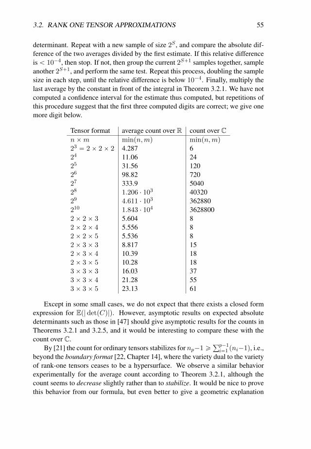
3.2. RANK ONE TENSOR APPROXIMATIONS 55
determinant. Repeat with a new sample of size 2S , and compare the absolute dif-ference of the two averages divided by the first estimate. If this relative differenceis ă 10´4, then stop. If not, then group the current 2S`1 samples together, sampleanother 2S`1, and perform the same test. Repeat this process, doubling the samplesize in each step, until the relative difference is below 10´4. Finally, multiply thelast average by the constant in front of the integral in Theorem 3.2.1. We have notcomputed a confidence interval for the estimate thus computed, but repetitions ofthis procedure suggest that the first three computed digits are correct; we give onemore digit below.
Tensor format average count over R count over Cnˆm minpn,mq minpn,mq23 “ 2ˆ 2ˆ 2 4.287 624 11.06 2425 31.56 12026 98.82 72027 333.9 504028 1.206 ¨ 103 4032029 4.611 ¨ 103 362880210 1.843 ¨ 104 36288002ˆ 2ˆ 3 5.604 82ˆ 2ˆ 4 5.556 82ˆ 2ˆ 5 5.536 82ˆ 3ˆ 3 8.817 152ˆ 3ˆ 4 10.39 182ˆ 3ˆ 5 10.28 183ˆ 3ˆ 3 16.03 373ˆ 3ˆ 4 21.28 553ˆ 3ˆ 5 23.13 61
Except in some small cases, we do not expect that there exists a closed formexpression for Ep|detpCq|q. However, asymptotic results on expected absolutedeterminants such as those in [47] should give asymptotic results for the counts inTheorems 3.2.1 and 3.2.5, and it would be interesting to compare these with thecount over C.
By [21] the count for ordinary tensors stabilizes for np´1 ěřp´1i“1 pni´1q, i.e.,
beyond the boundary format [22, Chapter 14], where the variety dual to the varietyof rank-one tensors ceases to be a hypersurface. We observe a similar behaviorexperimentally for the average count according to Theorem 3.2.1, although thecount seems to decrease slightly rather than to stabilize. It would be nice to provethis behavior from our formula, but even better to give a geometric explanation
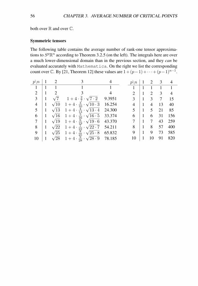
56 CHAPTER 3. AVERAGE NUMBER OF CRITICAL POINTS
both over R and over C.
Symmetric tensors
The following table contains the average number of rank-one tensor approxima-tions to SpRn according to Theorem 3.2.5 (on the left). The integrals here are overa much lower-dimensional domain than in the previous section, and they can beevaluated accurately with Mathematica. On the right we list the correspondingcount over C. By [21, Theorem 12] these values are 1`pp´1q`¨ ¨ ¨`pp´1qn´1.
pzn 1 2 3 41 1 1 1 12 1 2 3 43 1
?7 1` 4 ¨ 27 ¨
?7 ¨ 2 9.3951
4 1?
10 1` 4 ¨ 310 ¨
?10 ¨ 3 16.254
5 1?
13 1` 4 ¨ 413 ¨
?13 ¨ 4 24.300
6 1?
16 1` 4 ¨ 516 ¨
?16 ¨ 5 33.374
7 1?
19 1` 4 ¨ 619 ¨
?19 ¨ 6 43.370
8 1?
22 1` 4 ¨ 722 ¨
?22 ¨ 7 54.211
9 1?
25 1` 4 ¨ 825 ¨
?25 ¨ 8 65.832
10 1?
28 1` 4 ¨ 928 ¨
?28 ¨ 9 78.185
pzn 1 2 3 41 1 1 1 12 1 2 3 43 1 3 7 154 1 4 13 405 1 5 21 856 1 6 31 1567 1 7 43 2598 1 8 57 4009 1 9 73 58510 1 10 91 820
Chapter 4
Orthogonal and unitary tensordecomposition
57
58 CHAPTER 4. ODECO AND UDECO TENSORS
Unlike matrices, which always have a singular-value decomposition, higher-order tensors typically do not admit a decomposition in which the terms are pair-wise orthogonal. In this chapter we prove that orthogonally decomposable (odeco)tensors form a real-algebraic variety. In order to do this we associate an algebra toa tensor and show that if the tensor is orthogonally decomposable, then the algebrasatisfies certain polynomial identities. Conversely, we show that these identitiesimply the existence of an orthogonal decomposition. This chapter presents partsof the work of Boralevi, Draisma, Horobet and Robeva [8].
In general, tensor decomposition is NP-hard [25]. The decomposition of odecotensors, however, can be found efficiently. The vectors in the decomposition ofan odeco tensor are exactly the attraction points of the tensor power method andare called robust eigenvectors (see for instance [43]). Because of their efficientdecomposition, odeco tensors have been used in machine learning, in particularfor learning latent variables in statistical models [1].
4.1 Introduction and result
In this chapter we consider tensors in a tensor product V1 b ¨ ¨ ¨ b Vd of finite-dimensional vector spaces Vi over a fixed field K P tR,Cu, where the tensorproduct is also overK.We assume that each Vi is equipped with a positive-definiteinner product p¨|¨q, Hermitian if K “ C.
Definition 4.1.1. A tensor in V1b ¨ ¨ ¨ b Vd is called orthogonally decomposable(odeco, if K “ R) or unitarily decomposable (udeco, if K “ C) if it can bewritten as
kÿ
i“1
vi1 b ¨ ¨ ¨ b vid,
where for each j the vectors v1j , . . . , vkj are nonzero and pairwise orthogonal inVj .
The property above is also called “complete orthogonality” (see for instance[12, 32, 51]).
We use the adverb unitarily for K “ C to stress that we have fixed Hermi-tian inner products rather than symmetric bilinear forms. Note that orthogonalityimplies that the number k of terms is at most the minimum of the dimensions ofthe Vi, so odeco tensors form a rather low-dimensional subset of the space of alltensors. Next we consider tensor powers of a single, finite-dimensional K-spaceV.We write SymdpV q for the subspace of V bd consisting of all symmetric tensors,i.e., those fixed by all permutations of the tensor factors.
4.1. INTRODUCTION AND RESULT 59
Definition 4.1.2. A tensor in SymdpV q is called symmetrically odeco (ifK “ R)or symmetrically udeco (if K “ C) if it can be written as
kÿ
i“1
˘vbdi
where the vectors v1, . . . , vk are nonzero, pairwise orthogonal vectors in V.
The signs are only required when K “ R and d is even, as they can otherwisebe absorbed into the vi by taking a d-th root of ´1. See also the parametrization3.2.10. A symmetrically odeco or udeco tensor is symmetric and odeco or udecoin the earlier sense. The converse also holds; see Proposition 4.2.21.
The third scenario concerns the space AltdpV q Ď V bd consisting of all alter-nating tensors, i.e., those T for which πT “ sgn pπqT for each permutation π ofrds. The simplest alternating tensors are the alternating product tensors
v1 ^ ¨ ¨ ¨ ^ vd :“ÿ
πPSd
sgn pπqvπp1q b ¨ ¨ ¨ b vπpdq.
This tensor is nonzero if and only if v1, . . . , vd form a linearly independent set, andit changes only by a scalar factor upon replacing these vectors by another basis ofthe space xv1, . . . , vdy. We say that this subspace is represented by the alternatingproduct tensor.
Definition 4.1.3. A tensor in AltdpV q is called alternatingly odeco or alternat-ingly udeco if it can be written as
kÿ
i“1
vi1 ^ ¨ ¨ ¨ ^ vid,
where the k ¨ d vectors v11, . . . , vkd are nonzero and pairwise orthogonal.
Equivalently, this means that the tensor is a sum of k alternating product ten-sors that represent pairwise orthogonal d-dimensional subspaces of V ; by choosingorthogonal bases in each of these spaces one obtains a decomposition as above. Inparticular, k is at most tn{du. For d ě 3, alternatingly odeco tensors are not odecoin the ordinary sense unless they are zero; see Remark 4.2.23.
Proposition 4.1.4. [8, Proposition 7] For d ě 3, any (ordinary, symmetrically oralternatingly) odeco or udeco tensor has a unique orthogonal decomposition.
By quantifier elimination, it follows that the set of odeco or udeco tensors isa semi-algebraic set in V1 b ¨ ¨ ¨ b Vd, i.e., a finite union of subsets described by
60 CHAPTER 4. ODECO AND UDECO TENSORS
polynomial equations and (weak or strict) polynomial inequalities; here this spaceis considered as a real vector space even if K “ C. A simple compactness argu-ment (see Proposition [8, Proposition 6]) also shows that they form a closed subsetin the Euclidean topology, so that only weak inequalities are needed. However, thefollowing main result says that, in fact, only equations are needed.
Theorem 4.1.5 (Main theorem). For each integer d ě 3, for K P tR,Cu, andfor all finite-dimensional inner product spaces V1, . . . , Vd and V over K, theodeco/udeco tensors in V1 b ¨ ¨ ¨ b Vd, the symmetrically odeco/udeco tensors inSymdpV q, and the alternatingly odeco/udeco tensors in AltdpV q form real alge-braic varieties defined by polynomials of degree given in the following table.
Degrees of equations odeco (over R) udeco (over C)symmetric 2 (associativity) 3 (semi-associativity)ordinary 2 (partial associativity) 3 (partial semi-associativity)alternating 2 (Jacobi) and 4 (cross) 3 (Casimir) and 4 (cross)
Here the words between the parentheses refer to the types of conditions to be ful-filled by the algebras corresponding to odeco/udeco tensors in the different scenar-ios, as it will be explained in what follows.
4.2 Proof of main theorem
In this section we give the proof of the main theorem in the following way: firstwe prove the theorem for symmetric, ordinary and alternating odeco/udeco tensorsof order three, then we derive the theorem for ordinary higher order tensors fromthe order three case and we prove that a symmetric tensor is symmetrically ode-co/udeco if and only if it is odeco/udeco when is considered as an ordinary tensor.Finally we prove the theorem for alternating higher order tensors.
In all proofs below, we will encounter a finite-dimensional vector space Aover K “ R or C equipped with a positive-definite inner product p¨|¨q, as well as abi-additive product AˆAÑ A, px, yq ÞÑ x ¨y which is bilinear if K “ R and bi-semilinear ifK “ C. The product will be either commutative or anti-commutative.Moreover, the inner product will be compatible with the product in the sense thatpx ¨ y|zq “ pz ¨ x|yq. An ideal in pA, ¨q is a K-subspace I such that I ¨ A Ď I , bycommutativity we then also have A ¨ I Ď I and A is called simple if A ‰ t0u andA contains no nonzero proper ideals. We have the following well-known result.
Lemma 4.2.1. The orthogonal complement IK of any ideal I in A is an ideal, aswell. Consequently, A splits as a direct sum of pairwise orthogonal simple ideals.
4.2. PROOF OF MAIN THEOREM 61
4.2.1 Symmetrically odeco three tensors
In this subsection, we fix a finite-dimensional real inner product space V and char-acterize odeco tensors in Sym3pV q. We have Sym3pV q Ď V b3 – pV ˚qb2 b V,where the isomorphism comes from the linear isomorphism V Ñ V ˚, v ÞÑ pv|¨q.Thus a general tensor T P Sym3pV q gives rise to a bilinear map
V ˆ V Ñ V, pu, vq ÞÑ u ¨ v,
which has the following properties:
1. u ¨ v “ v ¨ u for all u, v P V (commutativity, which follows from the factthat T is invariant under permuting the first two factors); and
2. pu ¨ v|wq “ pu ¨ w|vq (compatibility with the inner product, which followsfrom the fact that T is invariant under permuting the last two factors).
Thus T gives V the structure of an R-algebra equipped with a compatible innerproduct. The following lemma describes the quadratic equations from the MainTheorem.
Lemma 4.2.2. If T is symmetrically odeco, then pV, ¨q is associative.
Proof. Write T “řki“1 v
b3i where v1, . . . , vk are pairwise orthogonal nonzero
vectors. Then we find, for x, y, z P V, that
x ¨ py ¨ zq “ x ¨
˜
ÿ
i
pvi|yqpvi|zqvi
¸
“ÿ
i
pvi|xqpvi|yqpvi|zqpvi|viq “ px ¨ yq ¨ z,
where we have used that pvi|vjq “ 0 for i ‰ j in the second equality.
Proposition 4.2.3. Conversely, if pV, ¨q is associative, then T is symmetricallyodeco.
Proof. By Lemma 4.2.1, V has an orthogonal decomposition V “À
i Ui wherethe subspaces Ui are (nonzero) simple ideals. Correspondingly, T decomposesas an element of
À
i Sym3pUiq. Thus it suffices to prove that each Ui is one-dimensional. This is certainly the case when the multiplication Ui ˆ Ui Ñ Uiis zero, because then any one-dimensional subspace of Ui is an ideal in V, henceequal to Ui by simplicity. If the multiplication map is nonzero, then pick an ele-ment x P Ui such that the multiplication Mx : Ui Ñ Ui, y ÞÑ x ¨ y is nonzero.Then kerMx is an ideal in V, because for z P V we have
x ¨ pkerMx ¨ zq “ px ¨ kerMxq ¨ z “ t0u,
62 CHAPTER 4. ODECO AND UDECO TENSORS
where we use associativity. By simplicity of Ui, kerMx “ t0u. Now define anew bilinear multiplication ˚ on Ui via y ˚ z :“ M´1
x py ¨ zq. This multiplicationis commutative, has x as a unit element, and we claim that it is also associative.Indeed,
ppx¨yq˚zq˚px¨vq “M´1x pM´1
x ppx¨yq¨zq¨px¨vqq “ y ¨z ¨v “ px¨yq˚pz˚px¨vqq,
where we used associativity and commutativity of ¨ in the second equality. Sinceany element is a multiple of x, this proves associativity. Moreover, pUi, ˚q is sim-ple; indeed, if I is ideal, then M´1
x pUi ¨ Iq Ď I and hence
Ui ¨ px ¨ Iq “ pUi ¨ xq ¨ I “ Ui ¨ I Ď x ¨ I,
so that x ¨ I is an ideal in pUi, ¨q; and therefore I “ t0u or I “ Ui.Now pUi, ˚q is a simple, associative R-algebra with 1, hence isomorphic to a
matrix algebra over a division ring. As it is also commutative, it is isomorphic toeither R or C. If it were isomorphic to C, then it would contain a square root of´1, i.e., an element y with y ˚ y “ ´x, so that y ¨ y “ ´x ¨ x. But then
0 ă px ¨ y|x ¨ yq “ py ¨ y|x ¨ xq “ ´px ¨ x|x ¨ xq ă 0,
a contradiction. We conclude that Ui is one-dimensional, as desired.
Lemma 4.2.2 and Proposition 4.2.3 imply the Main Theorem for symmetri-cally odeco three-tensors, because the identity x ¨ py ¨ zq “ px ¨ yq ¨ z expressingassociativity translates into quadratic equations for the tensor T.
Example 4.2.4. To see how the identities for associativity, in Lemma 4.2.2, trans-form into equations for symmetrically odeco tensors we consider 2ˆ2ˆ2 tensors.Let te1, e2u be an orthonormal basis of R2 and we represent a general element ofSym3pR2q by
T “ t3,0e1 b e1 b e1 ` t2,1pe1 b e1 b e2 ` e1 b e2 b e1 ` e2 b e1 b e1q
` t1,2pe1 b e2 b e2 ` e2 b e1 b e2 ` e2 b e2 b e1q ` t0,3e2 b e2 b e2.
Then the identities for associativity are translated into one real equation. Namely,if we write out the condition for associativity for all possible 3-tuples of te1, e2u,then we find one linearly independent equation among them, namely
f “ t21,2 ´ t2,1t0,3 ` t22,1 ´ t1,2t3,0.
The ideal generated by f is prime of real codimension 1. This equation agreeswith the one found by Robeva in [43, Equation 3.1].
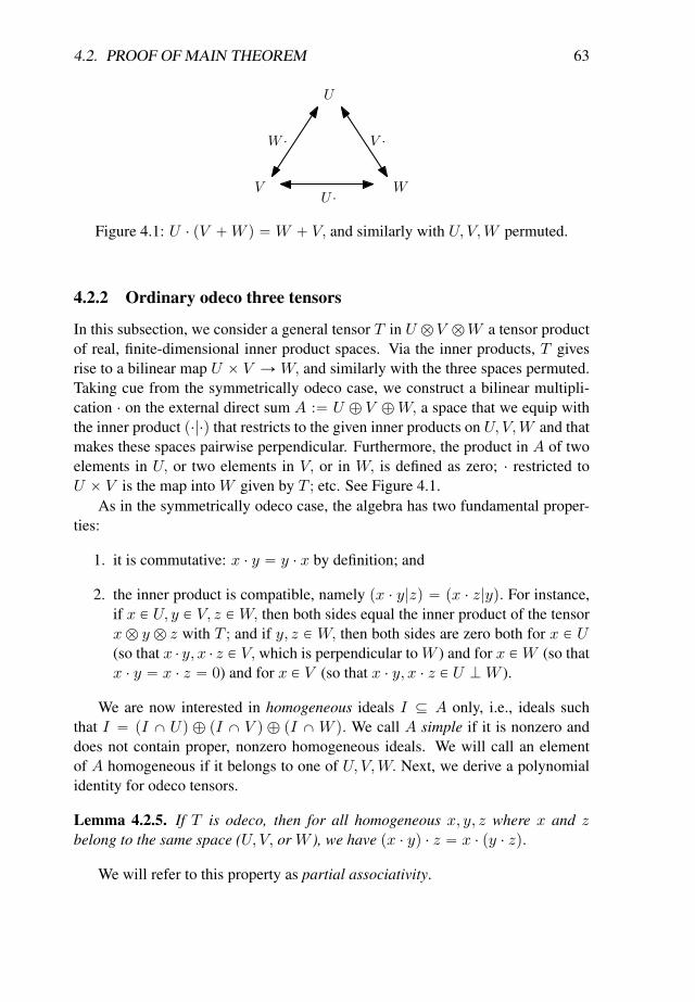
4.2. PROOF OF MAIN THEOREM 63
U
WV
W · V ·
U ·
Figure 4.1: U ¨ pV `W q “W ` V, and similarly with U, V,W permuted.
4.2.2 Ordinary odeco three tensors
In this subsection, we consider a general tensor T in U b V bW a tensor productof real, finite-dimensional inner product spaces. Via the inner products, T givesrise to a bilinear map U ˆ V Ñ W, and similarly with the three spaces permuted.Taking cue from the symmetrically odeco case, we construct a bilinear multipli-cation ¨ on the external direct sum A :“ U ‘ V ‘W, a space that we equip withthe inner product p¨|¨q that restricts to the given inner products on U, V,W and thatmakes these spaces pairwise perpendicular. Furthermore, the product in A of twoelements in U, or two elements in V, or in W, is defined as zero; ¨ restricted toU ˆ V is the map into W given by T ; etc. See Figure 4.1.
As in the symmetrically odeco case, the algebra has two fundamental proper-ties:
1. it is commutative: x ¨ y “ y ¨ x by definition; and
2. the inner product is compatible, namely px ¨ y|zq “ px ¨ z|yq. For instance,if x P U, y P V, z P W, then both sides equal the inner product of the tensorx b y b z with T ; and if y, z P W, then both sides are zero both for x P U(so that x ¨ y, x ¨ z P V, which is perpendicular to W ) and for x PW (so thatx ¨ y “ x ¨ z “ 0) and for x P V (so that x ¨ y, x ¨ z P U KW ).
We are now interested in homogeneous ideals I Ď A only, i.e., ideals suchthat I “ pI X Uq ‘ pI X V q ‘ pI XW q. We call A simple if it is nonzero anddoes not contain proper, nonzero homogeneous ideals. We will call an elementof A homogeneous if it belongs to one of U, V,W. Next, we derive a polynomialidentity for odeco tensors.
Lemma 4.2.5. If T is odeco, then for all homogeneous x, y, z where x and zbelong to the same space (U, V, or W ), we have px ¨ yq ¨ z “ x ¨ py ¨ zq.
We will refer to this property as partial associativity.
64 CHAPTER 4. ODECO AND UDECO TENSORS
Proof. If x, y, z all belong to the same space, then both products are zero. Other-wise, by symmetry, it suffices to check the case where x, z P U and y P V. LetT “
ř
i ui b vi b wi be an orthogonal decomposition of T. Then we have
px ¨ yq ¨ z “
˜
ÿ
i
pui|xqpvi|yqwi
¸
¨ z “ÿ
i
pui|xqpvi|yqpwi|wiqpz|uiq “ x ¨ py ¨ zq,
where we have used that pwi|wjq “ 0 for i ‰ j in the second equality.
Proposition 4.2.6. Conversely, if pA, ¨q is partially associative, then T is odeco.
Proof. By a version of Lemma 4.2.1 restricted to homogeneous ideals, A is thedirect sum of pairwise orthogonal, simple homogeneous ideals Ii. Accordingly, Tlies in
À
ipIiXUqbpIiXV qbpIiXW q. Thus it suffices to prove that T is odecounder the additional assumption that A itself is simple and that ¨ is not identicallyzero.
By symmetry, we may assume that V ¨ pU ` W q ‰ t0u. For u P U , letMu : V `W Ñ W ` V be multiplication with u. By commutativity and partialassociativity, the Mu, for u P U , all commute. By compatibility of the innerproduct, each Mu is symmetric with respect to the inner product on V `W , andhence orthogonally diagonalizable. Consequently, V `W splits as a direct sum ofpairwise orthogonal simultaneous eigenspaces
pV `W qλ :“ tv ` w P V `W | u ¨ pv ` wq “ λpuqpw ` vq for all u P Uu,
where λ runs over U˚.Now we prove that pV `W qλ ‘ rpV `W qλ ¨ pV `W qλs is a homogenous
ideal in A, for each λ P U˚. Recall that A “ U ‘´
À
µpV `W qµ
¯
. Suppose we
are given v ` w P pV `W qλ and v1 ` w1 P pV `W qµ with λ ‰ µ. Then v ` wand v1 ` w1 are perpendicular and for each u P V we have
pu|pv ` wq ¨ pv1 ` w1qq “ pu ¨ pv ` wq|v1 ` w1q “ λpuqpv ` w|v1 ` w1q “ 0,
hence pV `W qλ ¨ pV `W qµ “ 0. We have that U ¨ pV `W qλ Ď pV `W qλ, bydefinition. Then
U ¨ rpV `W qλ ¨ pV `W qλs “ 0,
since pV `W qλ ¨ pV `W qλ Ď U . Moreover
pV `W qλ ¨ rpV `W qλ ¨ pV `W qλs Ď pV `W qλ.
The only remaining thing to check is that pV `W qµ ¨ rpV `W qλ ¨ pV `W qλs iszero. Indeed take vµ ` wµ P Vµ `Wµ and v1λ ` w
1λ, v
2λ ` w
2λ P pV `W qλ, then
pvµ ` wµq ¨“
pv1λ ` w1λq ¨ pv
2λ ` w
2λq‰
“ pvµ ` wµq ¨ pv1λ ¨ w
2λ ` w
1λ ¨ v
2λq.
4.2. PROOF OF MAIN THEOREM 65
By commutativity the above expression equals
vµ ¨ pw2λ ¨ v
1λq ` vµ ¨ pw
1λ ¨ v
2λq ` wµ ¨ pv
1λ ¨ w
2λq ` wµ ¨ pv
2λ ¨ w
1λq,
which by partial associativity equals
v1λ ¨ pw2λ ¨ vµq ` v
2λ ¨ pw
1λ ¨ vµq ` w
2λ ¨ pv
1λ ¨ wµq ` w
1λ ¨ pv
2λ ¨ wµq “ 0,
by the fact that pV `W qλ ¨ pV `W qµ “ 0, for µ ‰ λ.We conclude that for each λ the space
pV `W qλ ‘ rpV `W qλ ¨ pV `W qλs
is a homogeneous ideal in A.By simplicity and the fact that Mu ‰ 0 for at least some u, A is equal to
this ideal for some nonzero λ P U˚. Pick an x P U such that λpxq “ 1, so thatx ¨ pv ` wq “ w ` v for all v P V, w P W . In particular, for v, v1 P V we havepMxv|Mxv
1q “ pM2xv|v
1q “ pv|v1q, so that the restrictions Mx : V Ñ W andMx : W Ñ V are mutually inverse isometries.
By the same construction, we find an element z PW such that
z ¨ pu` vq “ v ` u, for all u P U, v P V.
Let T 1 be the image of T under the linear map
Mz b IV bMx : U b V bW Ñ V b V b V,
via the isomorphism V bV bV » V ˚bV bV ˚. We claim that T 1 is symmetricallyodeco. Indeed, let ˚ : V ˆ V Ñ V denote the bilinear map associated to T 1. Weverify the conditions from subsection 4.2.1. First,
v˚v1 “ pz ¨vq ¨ px ¨v1q “ x ¨ ppz ¨vq ¨v1q “ x ¨ ppv1 ¨zq ¨vq “ px ¨vq ¨ pv1 ¨zq “ v1 ˚v,
where we have repeatedly used commutativity and partial associativity (e.g., in thesecond equality, to the elements z ¨ v, x belonging to the same space W ). Second,we have
pv˚v1|v2q “ ppz¨vq¨px¨v1q|v2q “ ppz¨vq|v1¨px¨v2qq “ pv|pz¨v1q¨px¨v2qq “ pv|v1˚v2q.
Hence T 1 is, indeed, and element of Sym3pV q. Finally, we have
pv ˚ v1q ˚ v2 “ pz ¨ ppz ¨ vq ¨ px ¨ v1qqq ¨ px ¨ v2q “ z ¨ ppx ¨ v2q ¨ ppz ¨ vq ¨ px ¨ v1qqq
“ z ¨ pppx ¨ v2q ¨ pz ¨ vqq ¨ px ¨ v1qq “ z ¨ ppv ˚ v2q ¨ px ¨ v1qq “ pv ˚ v2q ˚ v1,
which, together with commutativity, implies associativity of ˚. Hence T 1 is (sym-metrically) odeco by Proposition 4.2.6, and hence so is its image T under the tensorproduct Mz b IV bMx of linear isometries.
66 CHAPTER 4. ODECO AND UDECO TENSORS
4.2.3 Alternatingly odeco three tensors
In this subsection we consider a tensor T P Alt3pV q,where V is a finite-dimensionalreal vector space with inner product p¨|¨q.Via Alt3pV q Ď V b3 – pV ˚qb2bV sucha tensor gives rise to a bilinear map V ˆ V Ñ V, pu, vq ÞÑ ru, vs, which gives Vthe structure of an algebra. Now,
1. as the permutation p1, 2q maps T to ´T, we have ru, vs “ ´rv, us; and
2. as p2, 3q does the same, we have pru, vs|wq “ ´pru,ws|vq “ prw, us|vq, sothat the inner product is compatible with the product.
The following lemma gives the degree-two equations from the Main Theorem.
Lemma 4.2.7. If T is alternatingly odeco, then r¨, ¨s satisfies the Jacobi identity.
Proof. Let T “řki“1 ui ^ vi ^ wi be an orthogonal decomposition of T, and set
Vi :“ xui, vi, wiy. Then V splits as the direct sum of k ideals Vi and one furtherideal V0 :“ p
Àki“1 Viq
K. The restriction of the bracket to V0 is zero, so it sufficesto verify the Jacobi identity on each Vi. By scaling the bracket, which preservesboth the Jacobi identity and the set of alternatingly odeco tensors, we achieve thatui, vi, wi can be taken of norm one. Then we have
rui, vis “ wi, rvi, wis “ ui, and rwi, uis “ vi,
which we recognize as the multiplication table of R3 with the cross product ˆ,isomorphic to the Lie algebra so3pRq.
The following lemma gives the degree-four equations from the Main Theorem.
Lemma 4.2.8. If T is alternatingly odeco, then rx, rrx, ys, rx, zsss “ 0 for allx, y, z P V .
We will refer to this identity as the first cross product identity.
Proof. By the proof of Lemma 4.2.7, if T is odeco, then V splits as an orthogonaldirect sum of ideals V1, . . . , Vk that are isomorphic, as Lie algebras with compati-ble inner products, to scaled copies of R3 with the cross product, and possibly anadditional ideal V0 on which the multiplication is trivial. Thus it suffices to provethat the lemma holds for R3 with the cross product. But there it is immediate: ifrrx, ys, rx, zss is nonzero, then the two arguments span the plane orthogonal to x,hence their cross product is a scalar multiple of x.
We now prove the Main Theorem for alternatingly odeco three-tensors.
4.2. PROOF OF MAIN THEOREM 67
Proposition 4.2.9. Conversely, if the bracket r¨, ¨s on V satisfies the Jacobi identityand the first cross product identity, then T is alternatingly odeco.
Proof. By Lemma 4.2.1 the space V splits into pairwise orthogonal, simple idealsVi. Correspondingly, T lies in
À
i Alt3Vi, where the sum is over those Vi wherethe bracket is nonzero. These are simple real Lie algebras equipped with a com-patible inner product, hence compact Lie algebras. Let g be one of these, so gsatisfies the first cross product identity. Then so does the complex Lie algebragC :“ C b g, which is semisimple. For g – so3pRq, we have gC – sl2pCq, i.e.,the Dynkin diagram of gC has a single node. The classification of simple compactLie algebras (see, e.g., [31]) shows that, if g is not isomorphic to so3pRq, thenthe Dynkin diagram of gC contains at least one edge, so that gC contains a copyof sl3pCq. However, this 8-dimensional complex Lie algebra does not satisfy thecross product identity, as for instance
rE11 ´ E33, rrE11 ´ E33, E12s, rE11 ´ E33, E23sss “ 2E13 ‰ 0,
where Eij is the matrix with zeroes everywhere except for a 1 on position pi, jq.Hence g – so3pRq is three-dimensional, and T is alternatingly odeco.
4.2.4 Symmetrically udeco three tensors
In this subsection, V is a complex, finite-dimensional vector space equipped witha positive-definite Hermitian inner product p¨|¨q and T is an element of Sym3pV q.There is a canonical linear isomorphism V Ñ V s, v ÞÑ pv|¨q, where V s is thespace of semilinear functions V Ñ C. Through Sym3pV q Ď V b3 – pV sqb2 b V,the tensor T gives rise to a bi-semilinear product V ˆ V Ñ V, pu, vq ÞÑ u ¨ v.Moreover:
1. since T is invariant under permuting the first two factors, ¨ is commutative;and
2. since T it is invariant under permuting the last two factors, we find thatpu ¨ v|wq “ pu ¨w|vq. Note that, in this identity, both sides are semilinear inall three vectors u, v, w.
The following lemma gives the degree-three equations of the Main Theorem.
Lemma 4.2.10. If T is symmetrically udeco, then for all x, y, z, u P V we have
x ¨ py ¨ pz ¨ uqq “ z ¨ py ¨ px ¨ uqq and px ¨ yq ¨ pz ¨ uq “ px ¨ uq ¨ pz ¨ yq.
68 CHAPTER 4. ODECO AND UDECO TENSORS
We call a commutative operation ¨ satisfying the identities in the lemma semi-associative. It is clear that any commutative and associative operation is alsosemi-associative, but the converse does not hold. Note that, since the productis bi-semilinear, both sides of the first identity depend semilinearly on x, z, u butlinearly on y, while both parts of the second identity depend linearly on all ofx, y, z, u.
Proof. Let T “ř
i vb3i be an orthogonal decomposition of T. Then we have
z ¨ u “ÿ
i
pvi|zqpvi|uqvi
andy ¨ pz ¨ uq “
ÿ
i
pvi|yqpz|viqpu|viqpvi|viqvi
by the orthogonality of the vi. We stress that the coefficient pvi|zqpvi|uq has beentransformed into its complex conjugate pz|viqpu|viq. Next, we find
x ¨ py ¨ pz ¨ uqq “ÿ
i
pvi|xqpy|viqpvi|zqpvi|uqpvi|viqpvi|viqvi
and this expression is invariant under permuting x, z, u in any manner. This provesthe first identity.
For the second identity, we compute
px ¨ yq ¨ pz ¨ uq “ÿ
i
pvi|viq2px|viqpy|viqpz|viqpu|viqvi,
which is clearly invariant under permuting x, y, z, u in any manner.
Proposition 4.2.11. Conversely, if ¨ is semi-associative, then T is symmetricallyudeco.
In fact, in the proof we will only use the first identity. The second identity willbe used later on, for the case of ordinary udeco three-tensors.
Example 4.2.12. To see how the identities for semi-associativity, in Lemma 4.2.10,transform into equations for symmetrically udeco tensors we consider 2 ˆ 2 ˆ 2tensors. Let te1, e2u be an orthonormal basis of C2 and we represent a generalelement of Sym3pC2q by
T “ t3,0e1 b e1 b e1 ` t2,1pe1 b e1 b e2 ` e1 b e2 b e1 ` e2 b e1 b e1q
` t1,2pe1 b e2 b e2 ` e2 b e1 b e2 ` e2 b e2 b e1q ` t0,3e2 b e2 b e2.
4.2. PROOF OF MAIN THEOREM 69
Then the identities for semi-associativity are translated into two complex equa-tions. Namely, if we write out the condition for semi-associativity for all possible4-tuples of te1, e2u, then we find two linearly independent equations among them.If we separate the real and imaginary parts of these two complex equations thenwe get that the real algebraic variety of 2 ˆ 2 ˆ 2 symmetrically udeco tensorsis given by the following four real equations (note that they are invariant underconjugation):
f1 “´ t21,2t1,2 ` t0,3t2,1t1,2 ´ t1,2t
21,2 ´ t1,2t2,1t2,1 ` t0,3t3,0t2,1 ` t1,2t0,3t2,1´
t2,1t1,2t2,1 ´ t3,0t22,1 ´ t
22,1t3,0 ` t1,2t3,0t3,0 ` t2,1t0,3t3,0 ` t3,0t1,2t3,0;
f2 “´ t21,2t1,2 ` t0,3t2,1t1,2 ` t1,2t
21,2 ´ t1,2t2,1t2,1 ` t0,3t3,0t2,1 ´ t1,2t0,3t2,1`
t2,1t1,2t2,1 ` t3,0t22,1 ´ t
22,1t3,0 ` t1,2t3,0t3,0 ´ t2,1t0,3t3,0 ´ t3,0t1,2t3,0;
f3 “´ t21,2t0,3 ` t0,3t2,1t0,3 ´ t1,2t2,1t1,2 ` t0,3t3,0t1,2 ´ t0,3t
21,2 ´ t
22,1t2,1`
t1,2t3,0t2,1 ` t0,3t0,3t2,1 ´ t1,2t1,2t2,1 ´ t2,1t22,1 ` t1,2t0,3t3,0 ` t2,1t1,2t3,0;
f4 “´ t21,2t0,3 ` t0,3t2,1t0,3 ´ t1,2t2,1t1,2 ` t0,3t3,0t1,2 ` t0,3t
21,2 ´ t
22,1t2,1`
t1,2t3,0t2,1 ´ t0,3t0,3t2,1 ` t1,2t1,2t2,1 ` t2,1t22,1 ´ t1,2t0,3t3,0 ´ t2,1t1,2t3,0.
The polynomials f1, f2, f3 and f4 generate a real codimension 2 variety. We donot know whether the ideal generated by these polynomials is prime or not.
Proof of Proposition 4.2.11. By Lemma 4.2.1, V is the direct sum of pairwise or-thogonal, simple ideals Vi. Correspondingly, T lies in
À
i Sym3pViq. We want toshow that those ideals on which the multiplication is nonzero are one-dimensional.Thus we may assume that V itself is simple with nonzero product.
Then the elements x P V for which the semilinear mapMx : V Ñ V, y ÞÑ x¨yis identically zero form a proper ideal in V, which is zero by simplicity. Hence forany nonzero x P V the map Mx is nonzero.
Now consider, for nonzero x P V, the space W :“ kerMx. We claim thatW is a proper ideal. First, W also equals kerM2
x , because if M2xv “ 0, then
pM2xv|vq “ pxpxvq|vq “ pxv|xvq “ 0, so xv “ 0. We have
M2xpV ¨W q “ x ¨ px ¨ pV ¨W qq “ V ¨ px ¨ px ¨W qq “ t0u.
Here we used semi-associativity in the second equality. So V ¨W Ď kerM2x “W,
as claimed. Hence W is zero.Fixing any nonzero x P V, we define a new operation on V by
y ˚ z :“M´1x py ¨ zq.
70 CHAPTER 4. ODECO AND UDECO TENSORS
Since M´1x is semilinear, ˚ is bilinear, commutative, and has x as a unit element.
We claim that it is also associative. For this we need to prove that
v ¨M´1x pz ¨ yq “ z ¨M´1
x pv ¨ yq
holds for all y, z, v P V. Write y “ M2xy1, so that x ¨ px ¨ pz ¨ y1qq “ z ¨ y and
x ¨ px ¨ pv ¨ y1qq “ v ¨ y by semi-associativity. Then the equation to be proved reads
v ¨ px ¨ pz ¨ y1qq “ z ¨ px ¨ pv ¨ y1qq,
which is another instance of semi-associativity.Furthermore, any nonzero element y P V is invertible in pV, ˚q with inverse
M´1y px ¨ xq. We conclude that pV, ˚,`q is a finite-dimensional field extension of
C, hence equal to C.
4.2.5 Ordinary udeco three tensors
In this subsection, U, V,W are three finite-dimensional complex vector spacesequipped with Hermitian inner products p¨|¨q and T is a tensor in U b V b W.Then T gives rise to bi-semilinear maps U ˆ V Ñ W, V ˆ U Ñ W, etc. Likefor ordinary three-tensors in the real case, we equip A :“ U ‘ V ‘W with thebi-semilinear product ¨ arising from these maps and with the inner product whichrestricts to the given inner products on U, V, and W, and is zero on all other pairs.By construction:
1. pA, ¨q is commutative, and
2. a straightforward verification shows that the inner product is compatible.
Lemma 4.2.13. If T is udeco, then
1. for all u, u1, u2 P U and v P V we have u ¨ pu1 ¨ pu2 ¨ vqq “ u2 ¨ pu1 ¨ pu ¨ vqq;
2. for all u P U, v, v1 P V, and w PW we have u ¨pv ¨pw ¨v1qq “ w ¨pv ¨pu ¨v1qqand pu ¨ vq ¨ pw ¨ v1q “ pu ¨ v1q ¨ pw ¨ vq;
and the same relations hold with U, V,W permuted in any manner.
We call ¨ partially semi-associative if it satisfies these conditions.
Proof. Let T “ř
i ui b vi b wi be an orthogonal decomposition of T. Then wehave
u2 ¨ v “ÿ
i
pui|u2qpvi|vqwi,
4.2. PROOF OF MAIN THEOREM 71
u1 ¨ pu2 ¨ vq “ÿ
i
pui|u1qpu2|uiqpv|viqpwi|wiqvi, and
u ¨ pu1 ¨ pu2 ¨ vqq “ÿ
i
pui|uqpu1|uiqpui|u
2qpvi|vqpwi|wiqpvi|viqwi,
which is invariant under swapping u and u2. The second identity is similar. Forthe last identity, we have
pu ¨ vq ¨ pw ¨ v1q “ÿ
i
pu|uiqpv|viqpwi|wiqpw|wiqpv1|viqpui|uiq,
which is invariant under swapping v and v1.
The following proposition implies the Main Theorem for three-tensors over C.
Proposition 4.2.14. Conversely, if ¨ is partially semi-associative, then T is udeco.
Proof. By a version of Lemma 4.2.1 for homogeneous ideals I Ď A, i.e., those forwhich I “ pIXUq‘pIXV q‘pIXW q, A splits as a direct sum of nonzero, pair-wise orthogonal, homogeneous ideals Ii that each do not contain proper, nonzerohomogeneous ideals, and T lies in
À
ipIiXUq b pIiX V q b pIiXW q, where thesum is over those i on which the multiplication ¨ is nontrivial. Thus we may as-sume thatA itself is nonzero, contains no proper nonzero ideals, and has nontrivialmultiplication. We then need to prove that each of U, V,W is one-dimensional.
Without loss of generality, U ¨ V is a non-zero subset of W. The u P U forwhich the multiplication Mu : V `W ÑW `V, pv`wq ÞÑ u ¨w` u ¨ v is zeroform a homogeneous, proper ideal in A, which is zero by simplicity.
Pick an x P U, and let Q :“ kerMx. We want to prove that Q ‘ pQ ¨ Qq is aproper homogeneous ideal in A. First we have that kerMx equals kerM2
x because0 “ pxpxvq|vq “ pxv|xvq implies xv “ 0. Now U ¨Q Ď Q because
M2xpU ¨Qq “ x ¨ px ¨ pU ¨Qqq “ U ¨ px ¨ px ¨Qqq “ t0u
by partial semi-associativity.Next, we have pQ¨QK|Uq “ pQ¨U |QKq “ t0u, so thatQ¨QK “ t0u. Because
V `W “ Q‘pQKXpV `W qq we only need to check if V ¨ pQ ¨Qq Ď Q, whichis true since, for v P QX V and w P QXW, we have
x ¨ pV ¨ pw ¨ vqq “ w ¨ pV ¨ px ¨ vqq “ t0u
by partial semi-associativity. We have now proved that Q ‘ pQ ¨ Qq is a properhomogeneous ideal in A. Hence Q “ 0 by simplicity.
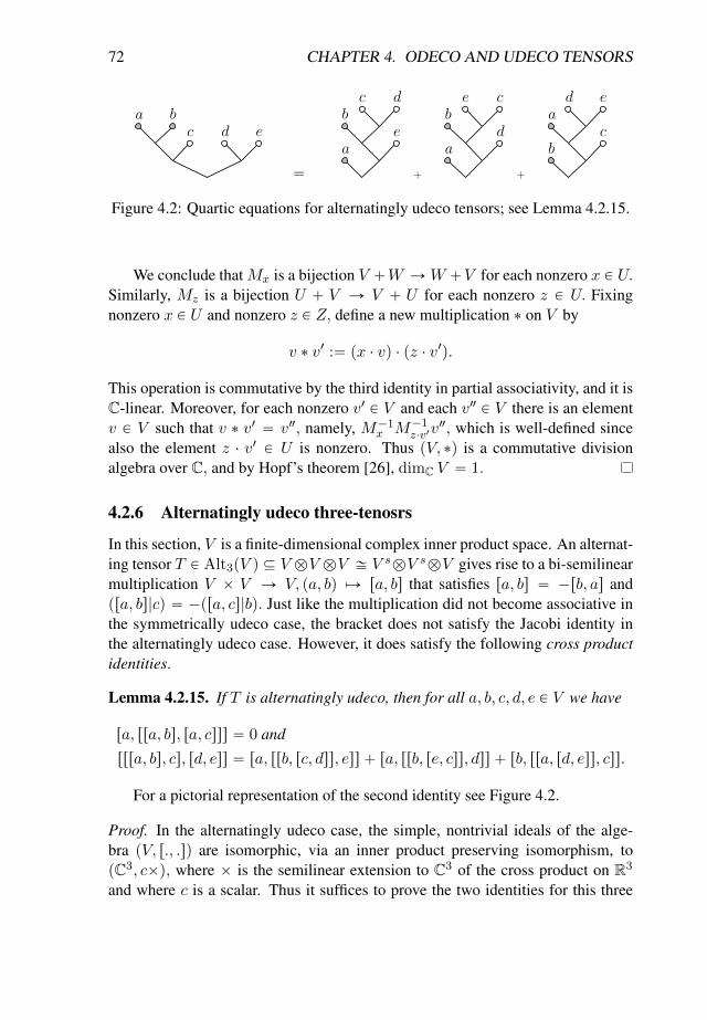
72 CHAPTER 4. ODECO AND UDECO TENSORS
a bc d e
=
a
bc d
e
+
a
bc
d
ea
bc
d e
+
Figure 4.2: Quartic equations for alternatingly udeco tensors; see Lemma 4.2.15.
We conclude thatMx is a bijection V `W ÑW `V for each nonzero x P U.Similarly, Mz is a bijection U ` V Ñ V ` U for each nonzero z P U. Fixingnonzero x P U and nonzero z P Z, define a new multiplication ˚ on V by
v ˚ v1 :“ px ¨ vq ¨ pz ¨ v1q.
This operation is commutative by the third identity in partial associativity, and it isC-linear. Moreover, for each nonzero v1 P V and each v2 P V there is an elementv P V such that v ˚ v1 “ v2, namely, M´1
x M´1z¨v1v
2, which is well-defined sincealso the element z ¨ v1 P U is nonzero. Thus pV, ˚q is a commutative divisionalgebra over C, and by Hopf’s theorem [26], dimC V “ 1.
4.2.6 Alternatingly udeco three-tenosrs
In this section, V is a finite-dimensional complex inner product space. An alternat-ing tensor T P Alt3pV q Ď V bV bV – V sbV sbV gives rise to a bi-semilinearmultiplication V ˆ V Ñ V, pa, bq ÞÑ ra, bs that satisfies ra, bs “ ´rb, as andpra, bs|cq “ ´pra, cs|bq. Just like the multiplication did not become associative inthe symmetrically udeco case, the bracket does not satisfy the Jacobi identity inthe alternatingly udeco case. However, it does satisfy the following cross productidentities.
Lemma 4.2.15. If T is alternatingly udeco, then for all a, b, c, d, e P V we have
ra, rra, bs, ra, csss “ 0 and
rrra, bs, cs, rd, ess “ ra, rrb, rc, dss, ess ` ra, rrb, re, css, dss ` rb, rra, rd, ess, css.
For a pictorial representation of the second identity see Figure 4.2.
Proof. In the alternatingly udeco case, the simple, nontrivial ideals of the alge-bra pV, r., .sq are isomorphic, via an inner product preserving isomorphism, topC3, cˆq, where ˆ is the semilinear extension to C3 of the cross product on R3
and where c is a scalar. Thus it suffices to prove the two identities for this three
4.2. PROOF OF MAIN THEOREM 73
dimensional algebra. Moreover, both identities are homogeneous in the sense thattheir validity for some pa, b, c, d, eq implies their validity when any one of the vari-ables is scaled by a complex number. Indeed, for the first identity this is clear,and for the second identity this follows since all four terms are semilinear in a, band linear in c, d, e. Hence both identities follow from their validity for the crossproduct and general a, b, c, d, e P R3.
The cross product identities yield real degree-four equations that vanish on theset of alternatingly odeco three-tensors. There are also degree-three equations,which arise as follows. Let µ : V b V Ñ V, pa b bq Ñ ra, bs be the semilinearmultiplication, and let, conversely, ψ : V Ñ V b V be the semilinear map deter-mined by pc|ra, bsq “ pab b|ψpcqq—note that both sides are linear in a, b, c. Thenlet H :“ µ ˝ ψ : V Ñ V. Being the composition of two semilinear maps, thisis a linear map, and it satisfies pHa|bq “ pψpaq|ψpbqq “ pa|Hbq. Hence H is apositive semidefinite Hermitian map.
Lemma 4.2.16. If T is alternatingly udeco, then rHx, ys “ rx,Hys for all x, y PV.
Proof. Let T “ř
i ui ^ vi ^ wi be an orthogonal decomposition of T. Then wehave
rHx, ys “ rµpÿ
i
pwi|xqui ^ vi ´ pvi|xqui ^ wi ` pui|xqvi ^ wiq, ys
“ÿ
i
r2pwi|xqpui|uiqpvi|viqwi ` 2pvi|xqpui|uiqpwi|wiqvi
` 2pui|xqpvi|viqpwi|wiqui, ys
“ 2ÿ
i
ppwi|xqpui|uiqpvi|viqpwi|wiqppui|yqvi ´ pvi|yquiq
` pvi|xqpui|uiqpwi|wiqpvi|viqppwi|yqui ´ pui|yqwiq
` pui|xqpvi|viqpwi|wiqpui|uiqppvi|yqwi ´ pwi|yqviqq.
Now we observe that the latter expression is skew-symmetric in x and y, so thisequals ´rHy, xs “ rx,Hys.
Remark 4.2.17. For a real, compact Lie algebra g, the positive semidefinite ma-trix H constructed above is a (negative) scalar multiple of the Casimir element inits adjoint action [31]; this is why we call the identity in the lemma the Casimiridentity. Complexifying g and its invariant inner product to a semilinear alge-bra with an invariant Hermitian inner product, we obtain an algebra satisfying thedegree-three equations of the lemma. Hence, since for dimV ě 8 there exist othercompact Lie algebras, these equations do not suffice to characterize alternatinglyudeco three-tensors in general, though perhaps they do so for dimV ď 7.
74 CHAPTER 4. ODECO AND UDECO TENSORS
In a Lie algebra, if ra, bs “ 0, then the left multiplications La : V Ñ V andLb : V Ñ V commute. This is not true in our setting, since the Jacobi identitydoes not hold, but the following statement does hold.
Lemma 4.2.18. Suppose that the bracket satisfies the second cross product iden-tity in Lemma 4.2.15, and let a, b, c P V be such that ra, cs “ rb, cs “ 0. Thenrra, bs, cs “ 0.
Proof. Compute the inner product
prra, bs, cs|rra, bs, csq “ ´prra, bs, rra, bs, css|cq “ prrra, bs, cs, ra, bss|cq
and use the identity to expand the first factor in the last inner product as
rrra, bs, cs, ra, bss “ ra, rrb, rc, ass, bss ` ra, rrb, rb, css, ass ` rb, rra, ra, bss, css.
Now each of the terms on the right-hand side is of the form ra, xs or rb, ys, andwe have pra, xs|cq “ ´pra, cs, xq “ 0 and similarly prb, xs|cq “ 0. Since the innerproduct is positive definite, this shows that rra, bs, cs “ 0, as claimed.
We now prove that our equations found so far suffice.
Proposition 4.2.19. Suppose that, conversely, T P Alt3pV q has the properties inLemmas 4.2.15 and 4.2.16. Then T is alternatingly udeco.
Proof. If a, b P V belong to distinct eigenspaces of the Hermitian linear map H,then the property that rHa, bs “ ra,Hbs implies that ra, bs “ 0. Moreover, a fixedeigenspace of H is closed under multiplication, as for a, b in the eigenspace witheigenvalue λ and c in the eigenspace with eigenvalue µ ‰ λ, we have
λpra, bs|cq “ prHa, bs|cq “ ´prHa, cs|bq “ ´µpra, cs|bq “ µpra, bs|cq,
and hence pra, bs|cq “ 0. Thus the eigenspaces of H are ideals. We may replaceV by one of these, so that H becomes a scalar. If the scalar is zero, then T is zeroand we are done, so we assume that it is nonzero, in which case we can scale T(even by a positive real number) to achieve that H “ 1.
Furthermore, by compatibility of the inner product and Lemma 4.2.1, V splitsfurther as a direct sum of simple ideals. So to prove the proposition, in additionto H “ 1, we may assume that V is a simple algebra and that the multiplicationis not identically zero; in this case it suffices to prove that V is three-dimensional.Let x P V be a non-zero element such that the semi-linear left multiplicationLx : V Ñ V has minimal possible rank. If its rank is zero, then xxy is an ideal,contrary to the assumptions. Hence V1 :“ LxV is a nonzero space, and we set
4.2. PROOF OF MAIN THEOREM 75
V0 :“ rV1, V1s, the linear span of all products of two elements from V1. We claimthat x P V0. For this, we note that V K1 “ kerLx and compute
pψpxq|V K1 b V q “ prVK1 , V s|xq “ prkerLx, xs|V q “ t0u.
Similarly, we find that pψpxq|V b V K1 q “ t0u, so ψpxq P V1 b V1 and therefore
x “ Hx “ µpψpxqq P rV1, V1s “ V0,
as claimed.By the first cross product identity in Lemma 4.2.15, we find that rx, V0s “ t0u.
This implies that pV0|V1q “ pV0|rx, V sq “ prx, V0s|V q “ t0u, so V0 K V1.Furthermore, by substituting x ` s for x in that same identity and taking the partquadratic in x, we find the identity
rs, rrx, as, rx, bsss ` rx, rrs, as, rx, bsss ` rx, rrx, as, rs, bsss “ 0.
A general element of rV, V0s is a linear combination of terms of the left-most shapein this identity, hence the identity shows that rV, V0s Ď V1. Moreover, substitutingfor s an element rrx, cs, rx, dss P V0 we find that the last two terms are zero, sincers, as P V1 and rx, rV1, V1ss “ t0u. Hence the first term is also zero, which showsthat rV0, V0s “ t0u.
Now let V2 be the orthogonal complement pV0 ‘ V1qK, so that V decom-
poses orthogonally as V0 ‘ V1 ‘ V2. We claim that V2 is an ideal. First, we haveprV0, V2s|V q “ pV2|rV0, V sq Ď pV2|V1q “ t0u, so rV0, V2s “ t0u. By the firstparagraph of the proof, x is contained in V0, hence in particular rx, V2s “ 0, so thatkerLx contains V0‘V2. For dimension reasons, equality holds: kerLx “ V0‘V2.Now Lemma 4.2.18 applied with c “ x yields that kerLx is closed under multi-plication, so in particular rV2, V2s Ď V0 ‘ V2. Since prV2, V2s|V0q “ t0u, we haverV2, V2s Ď V2. Furthermore, we have
prV1, V2s|V0 ‘ V1q “ pV2|V1 ‘ V0q “ t0u,
so that rV1, V2s Ď V2. This concludes the proof of the claim that V2 is an ideal. Bysimplicity of V, V2 “ t0u and hence V “ V0 ‘ V1.
Now consider any y P V0zt0u. Then kerLy Ě V0 ‘ V2, and hence equalityholds by maximality of dim kerLx. But we can show more: let v P V1 be an eigen-vector of the map pLx|V1q
´1pLy|V1q (which is linear since it is the composition oftwo semilinear maps), say with eigenvalue λ. Then ry, vs “ rx, λvs “ rλx, vs.This means that the element z :“ y ´ λx P V0 has kerLz Ě V0 ‘ V2, but alsov P kerLx. Hence the kernel of Lz is strictly larger than that of Lx, and thereforez “ 0. We conclude that y “ λx, and hence V0 is one-dimensional.
76 CHAPTER 4. ODECO AND UDECO TENSORS
Finally, consider a nonzero element z P V1. From rz, V1s Ď V0 “ xxy wefind that LzV is contained in xx, rz, xsyC, i.e., Lz has rank at most two. Hence,by minimality, the same holds for Lx. This means that dimV1 ď 2, and hencedimV “ dimpV0 ‘ V1q ď 3. Since T is nonzero, we find dimV “ 3, as desired.
4.2.7 Ordinary tensors
In this section, building on the case of order three, we prove the Main Theorem fortensors of arbitrary order.
Let V1, . . . , Vd be finite dimensional inner product spaces over K P tR,Cu.The key observation is the following. Let J1Y¨ ¨ ¨YJe “ t1, . . . , du be a partitionof t1, . . . , du. Then the natural flattening map
V1 b ¨ ¨ ¨ b Vd Ñ pâ
jPJ1
Vjq b ¨ ¨ ¨ b pâ
jPJe
Vjq
sends the set of order-d odeco/udeco tensors into the set of order-e odeco/udecotensors, where the inner product on each factor
Â
jPJ`Vj is the one induced from
the inner products on the factors. The following proposition gives a strong con-verse to this observation.
Proposition 4.2.20. Let T P V1b ¨ ¨ ¨bVd be a tensor, where d ě 4. Suppose thatthe flattenings of T with respect to the three partitions
(i) t1u, . . . , td´ 3u, td´ 2u, td´ 1, du,
(ii) t1u, . . . , td´ 3u, td´ 2, d´ 1u, tdu, and
(iii) t1u, . . . , td´ 3u, td´ 2, du, td´ 1u
are all odeco/udeco. Then so is T.
The lower bound of 4 in this proposition is essential, because any flattening ofa three-tensor is a matrix and hence odeco, but as we have seen in Section 4.2.2not every three-tensor is odeco.
Proof. As the first two flattenings are odeco, we have orthogonal decompositions
T “kÿ
i“1
Ti b ui bAi “rÿ
`“1
T 1` bB` b w`
where A1, . . . , Ak P Vd´1 b Vd are pairwise orthogonal and nonzero, and so areu1, . . . , uk P Vd´2, and the Ti are of the form zi1 b ¨ ¨ ¨ b zipd´3q where for each
4.2. PROOF OF MAIN THEOREM 77
j the zij , i “ 1, . . . are pairwise orthogonal and nonzero. Similarly for the factorsin the second expression. Contracting T with Ti in the first d ´ 3 factors yields asingle term on the left (here we use that d ą 3):
pTi|Tiqui bAi “rÿ
`“1
pT 1`|TiqB` b w`.
For an index ` such that pT 1`|Tiq is nonzero, by contracting with w` we find that B`is of rank one and, more specifically, of the form ui b v` with v` P Vd´1. Thereis at least one such index, since the left-hand side is nonzero. Moreover, since theui are linearly independent for distinct i, we find that the set of ` with pT 1`|Tiq ‰ 0is disjoint from the set defined similarly for another value of i. Hence, r ě k. Byswapping the roles of the two decompositions we also find the opposite equality,so that r “ k, and after relabelling we find Bi “ ui b vi for i “ 1, . . . , k andcertain nonzero vectors vi. Hence we find
T “kÿ
i“1
T 1i b ui b vi b wi,
where we do not yet know whether the vi are pairwise perpendicular. However,applying the same reasoning to the second and third decompositions in the lemma,we obtain another decomposition
T “kÿ
i“1
T 1i b u1i b v
1i b wi,
where we do know that the v1i are pairwise perpendicular (but not that the u1i are).Contracting with T 1i we find that, in fact, both decompositions are equal and the viare pairwise perpendicular, as required.
Proof of the Main Theorem for ordinary tensors. It follows from Lemma 4.2.5 andProposition 4.2.6, that ordinary odeco tensors of order three are characterized bydegree-two equations. Similarly, by Lemma 4.2.13 and Proposition 4.2.14, ordi-nary udeco tensors of order three are characterized by degree-three equations. ByProposition 4.2.20 and the remarks preceding it, a higher-order tensor is odeco(udeco) if and only if certain of its flattenings are odeco (udeco). Thus the equa-tions characterising lower-order odeco (udeco) tensors pull back, along linear maps,to equations characterising higher-order odeco (udeco) tensors.
4.2.8 Symmetric tensors
In this section, V is a finite-dimension vector space over K “ R or C.
78 CHAPTER 4. ODECO AND UDECO TENSORS
Proposition 4.2.21. For d ě 3, a tensor T P SymdpV q is symmetrically odeco(udeco) if and only if it is odeco (udeco) when considered as an ordinary tensor inV bd.
Proof. The “only if” direction is immediate, since a symmetric orthogonal de-composition is a fortiori an ordinary orthogonal decomposition. For the converse,consider an orthogonal decomposition
T “kÿ
i“1
vi1 b ¨ ¨ ¨ b vid,
where the vij are nonzero vectors, pairwise perpendicular for fixed j. Since T issymmetric, we have
T “ÿ
i
viπp1q b ¨ ¨ ¨ b viπpdq
for each π P Sd. By uniqueness of the decomposition (Proposition 4.1.4), theterms in this latter decomposition are the same, up to a permutation, as the termsin the original decomposition. In particular, the unordered cardinality-k sets ofprojective pointsQj :“ trv1js, . . . , rvkjsu Ď PV are identical for all j “ 1, . . . , d.Consider the integer k ˆ d-matrix A with entries in rks :“ t1, . . . , ku determinedby aij “ m if rvijs “ rvm1s. This matrix has all integers 1, . . . , k in each column,in increasing order in the first column, and furthermore has the property that foreach d ˆ d-permutation matrix π there exists a k ˆ k-permutation matrix σ suchthat σA “ Aπ. To conclude the proof we only need to prove the following. Claim.Let k ě 1 and d ě 3 be natural numbers. Let Sk act on Sdk diagonally from the leftby left multiplication and let Sd act on Sdk from the right by permuting the terms.Consider an element
A :“ pid, τ2, . . . , τdq P Sdk ,
where id is the identity permutation. Suppose that for each π P Sd there exists aσ P Sk such that σA “ Aπ. Then A “ pid, . . . , idq.
Proof of claim. For j P t2, . . . , du pick πj “ p1, jq to be the transpositionswitching 1 and j. By the property imposed on A there exists a σj such thatσjA “ Aπj . In particular, pAπjq1 “ τj equals pσjAq1 “ σj . So τj “ σj for allj P t2, . . . , du. Since d ě 3, one can pick an index l which is fixed by πj , so thatτl “ pσjAql “ σjτl. So then σj “ id “ τj . This concludes the proof of the claim,and thus that of Proposition 4.2.21.
Proof of the Main Theorem for symmetric tensors. By the preceding proposition,the equations for odeco tensors in V b¨ ¨ ¨bV pull back to equations characterisingsymmetrically odeco tensors in Symd V via the inclusion of the latter space intothe former. Thus the Main Theorem for symmetric tensors follows from the MainTheorem for ordinary tensors, proved in the previous subsection.
4.2. PROOF OF MAIN THEOREM 79
Remark 4.2.22. The proof of the Main Theorem in Section 4.2.2 for ordinaryodeco three-tensors relies on the proof for symmetrically odeco three-tensors, sothe proof above does not render that proof superfluous. On the other hand, theproof for ordinary udeco three-tensors does not rely on that for symmetricallyudeco three-tensors, so in view of the proof above the latter could have been leftout. We have decided to retain it for completeness.
Remark 4.2.23. The argument in the proposition also implies that an odeco/udecotensor in V bdzt0u with d ě 3 cannot be alternating: permuting tensor factors witha transposition must leave the decomposition intact up to a sign and a permutationof terms, but then the claim shows that in each term all vectors are equal, hencetheir alternating product is zero.
4.2.9 Alternating tensors
In this section we prove that an alternating tensor of order at least four is alternat-ingly odeco/udeco if and only if all its contractions with a vector are. Thus, let Vbe a vector space over K P tR,Cu and consider an orthogonal decomposition
T “kÿ
i“1
λivi1 ^ ¨ ¨ ¨ ^ vid (4.2.1)
of an alternatingly odeco tensor T P AltdV, where v11, . . . , vkd form an orthonor-mal set of vectors in V and where λi P K. The following lemmas are straightfor-ward exercises in differential geometry, and we omit their proofs.
Lemma 4.2.24. Suppose thatK “ R. Let d ě 3 and dk ď n :“ dimV. The setXof alternatingly odeco tensors in AltdV with exactly k terms in their orthogonaldecomposition is a smooth manifold of dimension k` 1
2dkp2n´ pk` 1qdq whosetangent space at a point T is the direct sum of the following spaces:
1.Àk
i“1pAltd´1Viq^V0 where Vi “ xvi1, . . . , vidy and V0 “ pV1‘¨ ¨ ¨‘VkqK;
2.Àk
i“1 AltdVi; and
3. xλipvi1 ^ ¨ ¨ ¨ ^ vml ^ ¨ ¨ ¨ ^ vidq ´ λmpvm1 ^ ¨ ¨ ¨ ^ vij ^ ¨ ¨ ¨ ^ vmdqy, with1 ď j, l ď d and i ‰ m, where vml replaces vij in the first term and viceversa in the second term.
The three summands are obtained as follows: X is the image of the Cartesianproduct of the manifold of k ¨ d-tuples of orthonormal vectors with pRzt0uqk via
ϕ : ppvijqpi,jqPrksˆrds, λq ÞÑÿ
i
λivi1 ^ ¨ ¨ ¨ ^ vid.
80 CHAPTER 4. ODECO AND UDECO TENSORS
Replacing a vij by a vij` εv0 with v0 P V0 yields the first summand. Replacing λiby λi ` ε yields the second summand, and infinitesimally rotating pvij , vmlq intopvij`εvml, vml´εvijq yields the last summand. The complex analogue of Lemma4.2.24 is the following.
Lemma 4.2.25. Suppose that K “ C. Let d ě 3 and 2k ď n :“ dimC V. The setX of alternatingly udeco tensors in AltdV with exactly k terms in their orthogonaldecomposition is a smooth manifold of dimension 2k ` dkp2n´ pk ` 1qdq whosetangent space at T is the direct sum of the following spaces:
1. the complex spaceÀk
i“1pAltd´1Viq ^ V0 where Vi “ xvi1, . . . , vidy andV0 “ pV1 ‘ ¨ ¨ ¨ ‘ Vkq
K;
2. the complex spaceÀk
i“1 AltdVi;
3. the real space
xλipvi1 ^ ¨ ¨ ¨ ^ vml ^ ¨ ¨ ¨ ^ vidq ´ λmpvm1 ^ ¨ ¨ ¨ ^ vij ^ ¨ ¨ ¨ ^ vmdqy,
with 1 ď j, l ď d and i ‰ m, where vml replaces vij in the first term andvice versa in the second term; and
4. the real space
xλipvi1 ^ ¨ ¨ ¨ ^ pivmlq ^ ¨ ¨ ¨ ^ vidq ` λmpvm1 ^ ¨ ¨ ¨ ^ pivijq ^ ¨ ¨ ¨ ^ vmdqy,
with 1 ď j, l ď d and i ‰ m, where ivml replaces vij in the first term andvice versa in the second term and where i P C is a square root of ´1.
The last summand arises from the infinitesimal unitary transformations send-ing puij , umlq to puij ` iuml, uml ` iuijq.
Proposition 4.2.26. Let V be a vector space over K P tR,Cu. Let d ě 3 andlet S P Altd`1V. Then S is alternatingly odeco (or udeco) if and only if for eachv0 P V the contraction pS|v0q of S with v0 in the last factor is an alternatinglyodeco (or udeco) tensor in AltdV.
Proof. The “only if” direction is immediate: contracting the terms in an orthog-onal decomposition of S with v0 yields an orthogonal decomposition for pS|v0q.Note that in this process the pairwise orthogonal pd ` 1q-spaces encoded by Sare replaced by their d-dimensional intersections with the hyperplane vK0 , and dis-carded if they happen to be contained in that hyperplane.
Conversely, assume that all contractions of S with a vector are alternatinglyodeco. Among all v0 P V choose one, say of norm 1, such that T :“ pS|v0q is
4.2. PROOF OF MAIN THEOREM 81
odeco with the maximal number of terms, say k, and let λi and the vij be as in(4.2.1). Then Ψ : v ÞÑ pS|vq is a real-linear map from an open neighbourhood ofv0 in V into the set X in the lemma, and hence its derivative at v0, which is theΨ itself, maps V into the tangent space described in the lemma. Since contractingwith v0 maps Altd`1V into Altdpv
K0 q, we may choose a basis v00, . . . , v0pn´kdq of
V0 from the lemma that starts with v00 :“ v0. Now we have
S “
˜
kÿ
i“1
λivi1 ^ ¨ ¨ ¨ ^ vid ^ v00
¸
` S2 “: S1 ` S2
where pS2|v00q “ 0. We have an orthonormal basis pvijqij of V where pi, jq runsthrough A :“ prks ˆ rdsq Y pt0u ˆ rn´ kdsq, where rks :“ t1, . . . , ku.
For a subset I Ď A we write vI for the vector in Altd`1V obtained as thewedge product of the vectors labelled by I (in some fixed linear order on A). Thevectors vI with |I| “ d ` 1 form a K-basis of Altd`1V, and similarly for thosewith |I| “ d. Now pS1|vq lies in the tangent space to X at T for all v (indeed, inthe sum of the first two summands in the lemma). Hence also pS2|vq must lie inthat tangent space. Expand S2 on the chosen basis:
S2 “ÿ
IĎA,|I|“d`1
cIvI .
We claim that cI “ 0 unless I contains one of the k sets tiuˆrds. Indeed, supposethat cI ‰ 0 and that I does not contain any of these k sets. Contracting vI with anyvα with α P I yields ˘vJ where J :“ Iztαu, hence vJ appears with a nonzerocoefficient in pS2|vαq. By the lemma we find that J must contain a pd´ 1q-subsetof at least one of the sets tiu ˆ rds. So in particular, there exists an i such thatI itself contains a pd ´ 1q-subset of tiu ˆ rds. Suppose first that this i is unique,say equal to i0. Then contracting vI with vi0,j with pi0, jq P I yields ˘vJ whereJ contains only at most d ´ 2 of the elements of each of the sets tiu ˆ rds, acontradiction with the lemma. So this i is not unique. Then I contains d ´ 1elements from each of at least two disjoint sets, so 2pd ´ 1q ď d ` 1, so d ď 3,and hence d “ 3—here we use that d ě 3. Without loss of generality, then,I “ tp1, 1q, p1, 2q, p2, 1q, p2, 2qu.Now contracting vI with v11 yields a scalar times˘v12 ^ v21 ^ v22, hence this term appears in pS|v11q. But (see the last one/twosummand/summands in the tangent space for the odeco/udeco case, respectively)this term can only appear in a tangent vector if also the term ˘v11 ^ v23 ^ v13appears—which is impossible after contracting with v11. This proves the claim.
We conclude that S can be written as
S “kÿ
i“1
vi1 ^ ¨ ¨ ¨ ^ vid ^ wi
82 CHAPTER 4. ODECO AND UDECO TENSORS
for suitable vectors wi satisfying pwi|v0q “ λi. Set Wi :“ Vi ` xwiy. We need toshow that the spaces W1, . . . ,Wk are pairwise perpendicular. For this, it sufficesto show that, for z in an open dense subset of V, the spaces W 1
i :“ Wi X zK arepairwise perpendicular. We choose this open subset such that
1. the contraction pS|zq has an orthogonal decomposition with k terms;
2. the k spaces W 1i are d-dimensional and linearly independent;
3. the tensor ppS|zq|v0q “ ˘ppS|v0q|zq P Altd´1V, which by assumption isalternatingly odeco, has a unique orthogonal decomposition.
By proposition 4.1.4, the last condition is void if d ą 3.Now, eachW 2i :“W 1
iXvK0
is contained in Vi, so thatW 2i KW 2
m for all i ‰ m.Now, by assumption, the tensor
pS|zq Pkà
i“1
AltdW1i
is alternatingly odeco with k terms. Let U1, . . . , Uk be the d-dimensional, pairwiseorthogonal spaces encoded by it. Then ppS|zq|v0q has an orthogonal decomposi-tion with terms in Altd´1pUi X v
K0 q. But we also have
ppS|zq|v0q Pkà
i“1
Altd´1W2i ,
where the W 2i are pairwise perpendicular. So, since we assumed that this orthogo-
nal decomposition is unique, after a permutation of the Ui we have UiXvK0 “W 2i .
Now let ui1, . . . , uid be an orthonormal basis of Ui, where the first pd´ 1q form abasis ofW 2
i . Extend with u01, . . . , u0pn´kdq to an orthonormal basis of V. Arguingwith respect to the basis puIq|I|“d, we find that the map V k Ñ AltdV that sendspy1, . . . , ykq to
řki“1 ui1 ^ ¨ ¨ ¨ ^ uipd´1q ^ yi is injective. Since
pS|zq “kÿ
i“1
µiui1 ^ ¨ ¨ ¨ ^ uid “kÿ
i“1
µ1iui1 ^ ¨ ¨ ¨ ^ uipd´1q ^ w1i
for suitable w1i P W1i and nonzero scalars µi, µ1i, we find that W 1
i “ Ui, and hencethe W 1
i are pairwise perpendicular, as desired.
Proof of the Main Theorem for alternating tensors. In Lemmas 4.2.7 and 4.2.8 andProposition 4.2.9 we found that an alternating three-tensor is alternatingly odeco ifand only if it satisfies certain polynomial equations of degrees 2 and 4. Correspon-dingly, Proposition 4.2.19 settles the Main Theorem for alternatingly udeco three-tensors. Proposition 4.2.26 yields that the pullbacks of the real polynomial equa-tions characterising alternatingly odeco/udeco d-tensors along real-linear maps

4.2. PROOF OF MAIN THEOREM 83
yield equations characterising alternatingly odeco/udeco pd ` 1q-tensors. Thesepullbacks have the same degrees as the original equations.

84 CHAPTER 4. ODECO AND UDECO TENSORS

Chapter 5
Algebraic boundary of matricesof nonnegative rank at most three
85
86 CHAPTER 5. NONNEGATIVE RANK
The r-th mixture model M of two discrete random variables X and Y ex-presses the conditional independence of X and Y , given a third (hidden) variableZ, where Z has k “ 1, . . . , r states. Assuming that X has m and Y has n states,their joint distribution is written as the sum of r rank-one nonnegative m ˆ n-matrices (i.e. of nonnegative rank at most r.), expressing that X and Y are inde-pendent, given that Z “ k, with k “ 1, . . . , r. So the joint distribution is expressedas an mˆ n-matrix of nonnegative rank at most r.
A collection of i.i.d. samples from a joint distribution is recorded in a nonneg-ative matrix U “ puijqi,j , with 1 ď i ď m and 1 ď j ď n. Here uij is the numberof observations in the sample with X “ i and Y “ j. To fit the model to the dataU one can use the Expectation–Maximization (EM) algorithm [40][Section 1.3].The EM algorithm aims to maximize the log-likelihood function of the model. Indoing so, it approximates the data matrix U with a product of nonnegative matricespU :“ A ¨ B, where A has r columns and B has r rows, hence the product is ofnonnegative rank at most r. One of the drawbacks of this algorithm, as Fienberg[16] pointed out, is that the optimal matrix pU either lies in the relative interior ofM or it lies in the model’s topological boundary BM (to be defined later).
If pU lies in the interior ofM, then it is a critical point for the likelihood func-tion on the manifold of rank r matrices. Things are more difficult when pU lies inthe boundary BM. In that case, pU is generally not a critical point for the likelihoodfunction in the manifold of rank r matrices [33].
In order to test algebraically wether pU lies on the topological boundary ofthe model one needs to consider the algebraic closure of it. This work was doneKubjas-Robeva-Sturmfels[33] and led to a conjecture [33, Conjecture 6.4], re-garding the algebraic boundary of matrices of nonnegative rank at most three.This chapter presents a proof of this conjecture based on the work of Eggermont,Horobet and Kubjas [20] and we conclude by some observations and conjecturesregarding the algebraic boundary for r ě 3.
Theorem 5.0.27 ([33], Conjecture 6.4). Let m ě 4, n ě 3 and consider a non-trivial irreducible component of the algebraic boundary of the semialgebraic set ofmˆ n matrices of nonnegative rank at most 3. The prime ideal of this componentis minimally generated by
`
m4
˘`
n4
˘
quartics, namely the 4 ˆ 4-minors, and eitherby
`
m3
˘
sextics that are indexed by subsets ti, j, ku of t1, 2, . . . ,mu or`
n3
˘
sexticsthat are indexed by subsets ti, j, ku of t1, 2, . . . , nu.
5.1 Definitions
We denote the space of m ˆ n matrices over R by Mmˆn. For a fixed r we willdenote by Mďr
mˆn the variety of m ˆ n matrices of rank at most r. Moreover we
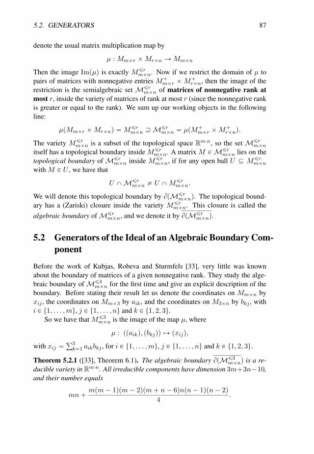
5.2. GENERATORS 87
denote the usual matrix multiplication map by
µ : Mmˆr ˆMrˆn ÑMmˆn
Then the image Impµq is exactly Mďrmˆn. Now if we restrict the domain of µ to
pairs of matrices with nonnegative entries M`mˆr ˆM`
rˆn, then the image of therestriction is the semialgebraic set Mďr
mˆn of matrices of nonnegative rank atmost r, inside the variety of matrices of rank at most r (since the nonnegative rankis greater or equal to the rank). We sum up our working objects in the followingline:
µpMmˆr ˆMrˆnq “Mďrmˆn ĚMďr
mˆn “ µpM`mˆr ˆM
`rˆnq.
The variety Mďrmˆn is a subset of the topological space Rm¨n, so the set Mďr
mˆn
itself has a topological boundary inside Mďrmˆn. A matrix M PMďr
mˆn lies on thetopological boundary ofMďr
mˆn inside Mďrmˆn, if for any open ball U Ď Mďr
mˆn
with M P U , we have that
U XMďrmˆn ‰ U XMďr
mˆn.
We will denote this topological boundary by BpMďrmˆnq. The topological bound-
ary has a (Zariski) closure inside the variety Mďrmˆn. This closure is called the
algebraic boundary ofMďrmˆn, and we denote it by BpMďr
mˆnq.
5.2 Generators of the Ideal of an Algebraic Boundary Com-ponent
Before the work of Kubjas, Robeva and Sturmfels [33], very little was knownabout the boundary of matrices of a given nonnegative rank. They study the alge-braic boundary ofMď3
mˆn for the first time and give an explicit description of theboundary. Before stating their result let us denote the coordinates on Mmˆn byxij , the coordinates on Mmˆ3 by aik, and the coordinates on M3ˆn by bkj , withi P t1, . . . ,mu, j P t1, . . . , nu and k P t1, 2, 3u.
So we have that Mď3mˆn is the image of the map µ, where
µ : ppaikq, pbkjqq ÞÑ pxijq,
with xij “ř3k“1 aikbkj , for i P t1, . . . ,mu, j P t1, . . . , nu and k P t1, 2, 3u.
Theorem 5.2.1 ([33], Theorem 6.1). The algebraic boundary BpMď3mˆnq is a re-
ducible variety in Rm¨n. All irreducible components have dimension 3m`3n´10,and their number equals
mn`mpm´ 1qpm´ 2qpm` n´ 6qnpn´ 1qpn´ 2q
4.
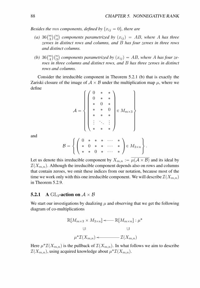
88 CHAPTER 5. NONNEGATIVE RANK
Besides the mn components, defined by txij “ 0u, there are
(a) 36`
m3
˘`
n4
˘
components parametrized by pxijq “ AB, where A has threezeroes in distinct rows and columns, and B has four zeroes in three rowsand distinct columns.
(b) 36`
m4
˘`
n3
˘
components parametrized by pxijq “ AB, where A has four ze-roes in three columns and distinct rows, and B has three zeroes in distinctrows and columns.
Consider the irreducible component in Theorem 5.2.1 (b) that is exactly theZariski closure of the image of A ˆ B under the multiplication map µ, where wedefine
A “
$
’
’
’
’
’
’
’
’
’
&
’
’
’
’
’
’
’
’
’
%
¨
˚
˚
˚
˚
˚
˚
˚
˚
˚
˝
0 ˚ ˚
0 ˚ ˚
˚ 0 ˚
˚ ˚ 0˚ ˚ ˚...
. . ....
˚ ˚ ˚
˛
‹
‹
‹
‹
‹
‹
‹
‹
‹
‚
PMmˆ3
,
/
/
/
/
/
/
/
/
/
.
/
/
/
/
/
/
/
/
/
-
and
B “
$
&
%
¨
˝
0 ˚ ˚ ˚ ¨ ¨ ¨ ˚
˚ 0 ˚ ˚ ¨ ¨ ¨ ˚
˚ ˚ 0 ˚ ¨ ¨ ¨ ˚
˛
‚PM3ˆn
,
.
-
.
Let us denote this irreducible component by Xm,n :“ µpAˆ Bq and its ideal byIpXm,nq. Although the irreducible component depends also on rows and columnsthat contain zeroes, we omit these indices from our notation, because most of thetime we work only with this one irreducible component. We will describe IpXm,nq
in Theorem 5.2.9.
5.2.1 A GL3-action on Aˆ BWe start our investigations by dualizing µ and observing that we get the followingdiagram of co-multiplications
RrMmˆ3 ˆM3ˆns RrMmˆns : µ˚oo
µ˚IpXm,nq
Ď
IpXm,nq
Ď
oo
Here µ˚IpXm,nq is the pullback of IpXm,nq. In what follows we aim to describeIpXm,nq, using acquired knowledge about µ˚IpXm,nq.
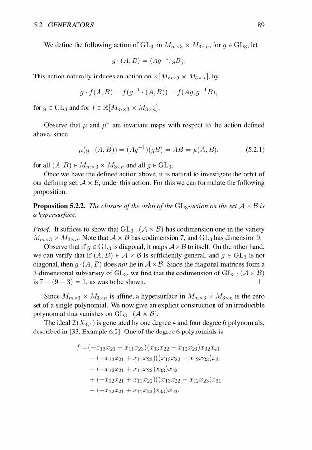
5.2. GENERATORS 89
We define the following action of GL3 on Mmˆ3 ˆM3ˆn, for g P GL3, let
g ¨ pA,Bq “ pAg´1, gBq.
This action naturally induces an action on RrMmˆ3 ˆM3ˆns, by
g ¨ fpA,Bq “ fpg´1 ¨ pA,Bqq “ fpAg, g´1Bq,
for g P GL3 and for f P RrMmˆ3 ˆM3ˆns.
Observe that µ and µ˚ are invariant maps with respect to the action definedabove, since
µpg ¨ pA,Bqq “ pAg´1qpgBq “ AB “ µpA,Bq, (5.2.1)
for all pA,Bq PMmˆ3 ˆM3ˆn and all g P GL3.Once we have the defined action above, it is natural to investigate the orbit of
our defining set,AˆB, under this action. For this we can formulate the followingproposition.
Proposition 5.2.2. The closure of the orbit of the GL3-action on the set Aˆ B isa hypersurface.
Proof. It suffices to show that GL3 ¨ pA ˆ Bq has codimension one in the varietyMmˆ3 ˆM3ˆn. Note that Aˆ B has codimension 7, and GL3 has dimension 9.
Observe that if g P GL3 is diagonal, it mapsAˆB to itself. On the other hand,we can verify that if pA,Bq P A ˆ B is sufficiently general, and g P GL3 is notdiagonal, then g ¨ pA,Bq does not lie inAˆB. Since the diagonal matrices form a3-dimensional subvariety of GL3, we find that the codimension of GL3 ¨ pAˆ Bqis 7´ p9´ 3q “ 1, as was to be shown.
Since Mmˆ3 ˆM3ˆn is affine, a hypersurface in Mmˆ3 ˆM3ˆn is the zeroset of a single polynomial. We now give an explicit construction of an irreduciblepolynomial that vanishes on GL3 ¨ pAˆ Bq.
The ideal IpX4,4q is generated by one degree 4 and four degree 6 polynomials,described in [33, Example 6.2]. One of the degree 6 polynomials is
f “p´x13x21 ` x11x23qpx13x22 ´ x12x23qx32x41
´ p´x13x21 ` x11x23qppx13x22 ´ x12x23qx31
´ p´x12x21 ` x11x22qx33qx42
` p´x12x21 ` x11x22qppx13x22 ´ x12x23qx31
´ p´x12x21 ` x11x22qx33qx43.
90 CHAPTER 5. NONNEGATIVE RANK
For m,n ě 4 the pull-back µ˚f factors as
pb13b22b31 ´ b12b23b31 ´ b13b21b32 ` b11b23b32 ` b12b21b33 ´ b11b22b33qf6,3,
with f6,3 a homogeneous degree p6, 3q-polynomial with 330 terms in the variablesai,k and bk,j with i P t1, . . . ,mu, j P t1, . . . , nu, and k P t1, 2, 3u.
By direct computations, one can check that f6,3 vanishes on A ˆ B and thefollowing lemma will imply that it vanishes on GL3 ¨ pAˆ Bq.
Lemma 5.2.3. The polynomial f6,3 is SL3-invariant. Moreover, for any g P GL3,we have g ¨ f6,3 “ detpgqf6,3.
Proof. Note that
D “ pb13b22b31 ´ b12b23b31 ´ b13b21b32 ` b11b23b32 ` b12b21b33 ´ b11b22b33q
is a 3ˆ 3-determinant, and hence it is SL3-invariant. Moreover, we have
pg ¨DqpBq “ Dpg´1Bq “ detpgq´1DpBq,
for any g P GL3 and B P B. Moreover, µ˚f is non-zero and GL3-invariant, by(5.2.1). So we have
Df6,3 “ µ˚f “ g ¨ µ˚f “ pg ¨Dqpg ¨ f6,3q “ pdetpgq´1Dqpg ¨ f6,3q,
for any g P GL3. It follows that we must have
g ¨ f6,3 “ detpgqf6,3.
In particular f6,3 is SL3-invariant.
Since f6,3 vanishes on Aˆ B, we immediately have the following corollary.
Corollary 5.2.4. The ideal of the set GL3 ¨ pAˆ Bq is xf6,3y.
Proof. By Proposition 5.2.2, the set GL3 ¨ pAˆ Bq is a hypersurface. By theprevious lemma, the polynomial f6,3 vanishes on GL3 ¨ pA ˆ Bq, since for anypA,Bq P Aˆ B and any g P GL3, we have
f6,3pAg´1, gBq “ pg´1 ¨ f6,3qpA,Bq “ detpgq´1f6,3pA,Bq “ detpgq´1 ¨ 0 “ 0.
One can easily check that f6,3 is irreducible, so the set GL3 ¨ pAˆ Bq must be thezero set of f6,3, and hence its ideal, which is the ideal of GL3 ¨ pA ˆ Bq as well,must be xf6,3y.
5.2. GENERATORS 91
5.2.2 The ideal of Xm,n
In what follows we will relate the ideal of GL3 ¨ pA ˆ Bq with the pull-back ofthe ideal of Xm,n. To do this we formulate two technical lemmas. The first onecontains the algebraic geometric essence of the proofs which follow, the other onecontains the representation theory.
Lemma 5.2.5. Let S be a subset of Mmˆ3 ˆM3ˆn, let Y be a subset of Mmˆn,and suppose µpSq is a Zariski dense subset of Y . Then µ˚IpY q “ IpSqXImpµ˚q.
Proof. Since µpSq is dense in Y , applying µ˚ we have
µ˚pIpµpSqqq “ µ˚pIpY qq.
It remains to prove that µ˚pIpµpSqqq “ IpSq X Impµ˚q. For this take an elementf of IpµpSqq, so for any pA,Bq P S we have that µ˚fpA,Bq “ fpµpA,Bqq “ 0,hence
µ˚pIpµpSqqq Ď IpSq X Impµ˚q.
Conversely take f “ µ˚f 1 in IpSq X Impµ˚q, so for any pA,Bq P S we havethat 0 “ fpA,Bq “ pµ˚f 1qpA,Bq “ f 1pµpA,Bqq, hence f 1 P IpµpSqq andtherefore
µ˚pIpµpSqqq Ě IpSq X Impµ˚q.
So we find that µ˚pIpY qq “ IpSq X Impµ˚q.
Lemma 5.2.6. The image of µ˚ is equal to RrMmˆ3 ˆM3ˆnsGL3 .
Proof. First, observe that for any f P RrMmˆns, any pA,Bq P Mmˆ3 ˆM3ˆn,and any g P GL3, we have
g ¨ pµ˚fqpA,Bq “ fpµpg ¨ pA,Bqqq “ fpµpA,Bqq “ µ˚fpA,Bq,
and hence Impµ˚q Ď RrMmˆ3 ˆM3ˆnsGL3 .
To prove the other inclusion, we refer to the First Fundamental theorem forGL3 (see for instance [42, Chapter 9, Section 1.4, Theorem 1]), which states thatthe GL3-invariant polynomials of RrMm,3 ˆ M3,ns are generated by the innerproducts
3ÿ
k“1
ai,kbk,j ,
for all 1 ď i ď m and 1 ď j ď n. Since these are simply the µ˚pxi,jq, we findthat Impµ˚q Ě RrMmˆ3 ˆM3ˆns
GL3 , which completes the proof.
Now as promised the following lemma relates µ˚IpXm,nq to GL3 ¨ pAˆ Bq.
92 CHAPTER 5. NONNEGATIVE RANK
Lemma 5.2.7. The pull-back of the ideal IpXm,nq is exactly xf6,3yGL3 .
Proof. We have that µpGL3 ¨ pA ˆ Bqq “ µpA ˆ Bq is dense in Xmˆn. ByLemma 5.2.5 (setting S “ GL3 ¨ pAˆ Bq and Y “ Xm,n) we get
µ˚IpXm,nq “ IpGL3 ¨ pAˆ Bqq X Impµ˚q.
Then applying Corollary 5.2.4 for the structure of GL3 ¨ pAˆBq and Lemma 5.2.6for pull-back of µ, we get that
µ˚IpXm,nq “ xf6,3y X RrMmˆ3 ˆM3ˆnsGL3 ,
which finishes the proof.
We continue investigating the structure of xf6,3yGL3 . For this we introduce thefollowing notation. For i “ pi, j, kq an ordered triple of elements in t1, . . . , nu,
we denote detB,i “ det
ˆ
b1i b1j b1kb2i b2j b2kb3i b3j b3k
˙
. Analogously, for i “ pi, j, kq an ordered
triple of elements in t1, . . . ,mu, we denote detA,i “ det´ ai1 ai2 ai3aj1 aj2 aj3ak1 ak2 ak3
¯
.The following proposition is the main result of this part, describing explicitly
the pull-back of IpXm,nq.
Proposition 5.2.8. We have
µ˚IpXm,nq “
#
ÿ
i
f6,3 detB,i
hi : hi P RrMmˆ3 ˆM3ˆnsGL3
+
.
Moreover, the f6,3 detB,i are GL3-invariant. Here, i runs over the ordered triplesof elements in t1, . . . , nu.
Proof. First by Lemma 5.2.7 we have that µ˚IpXm,nq “ xf6,3yGL3 , then we recall
that, by Lemma 5.2.3, f6,3 is SL3-invariant and that for any g P GL3 we haveg ¨ f6,3 “ detpgqf6,3. Therefore, any GL3-invariant element f of xf6,3y, has theform
f “ f6,3h,
with h an SL3-invariant polynomial satisfying g ¨h “ detpgq´1h for any g P GL3.By the First Fundamental Theorem for SLn (see for instance [42, Chapter 11,
Section 1.2, Theorem 3]) we know that h can be expressed in terms of the detA,i,the detB,i and the scalar products
ř
k ai,kbk,j . Observe that GL3 acts trivially onthe
ř
k ai,kbk,j , and acts on the detA,i and detB,i by g ¨detA,i “ detpgq detA,i andg ¨ detB,i “ detpgq´1 detB,i. The polynomial ring generated by these elements istherefore Z-graded, where the part of degree d is the part of the ring on which anyg acts by multiplication with detpgqd.
5.2. GENERATORS 93
Since g ¨ h “ detpgq´1h, it follows that h has degree ´1, and hence we canexpress it in the form
ÿ
i
detB,i ¨ hi,
where the hi are of degree 0, and hence are GL3-invariant polynomials.Then our f has the form
f “ÿ
i
pf6,3detB,iq ¨ hi, with hi P RrMm,3 ˆM3,nsGL3 .
So any f P xf6,3yGL3 can be expressed in the desired form, and each elementof this form is GL3-invariant. Moreover, the f6,3 detB,i are GL3-invariant, as wasto be shown.
Finally we have arrived at the point to draw conclusions about the generators ofIpXm,nq, using the knowledge we acquired about µ˚IpXm,nq. Take an arbitraryelement f of IpXm,nq. By Proposition 5.2.8, the polynomial µ˚f can be writtenas
µ˚f “ÿ
i
pf6,3detB,iqhi,
for some hi P RrMm,3ˆM3,nsGL3 . For each i, fix fi such that µ˚fi “ f6,3detB,i.
Since RrMm,3 ˆM3,nsGL3 is the image of µ˚ (by Lemma 5.2.6), there exist
αi, such that µ˚αi “ hi for each i. This way finally we get that
µ˚f “ µ˚
˜
ÿ
i
fiαi
¸
.
And finally this reads as
f ´ÿ
i
fiαi P Kerpµ˚q.
By the Second Fundamental Theorem for the general linear group (see for instance[42, Chapter 13, Section 8.1, Theorem 1]) the kernel of µ˚ is generated by the 4ˆ4determinants detj,k of matrices in Mm,n (where j, respectively k, is an ordered 4-tuple of elements in t1, . . . ,mu, respectively in t1, . . . , nu, and the determinant isdefined as one would expect), so we conclude that
IpXm,nq Ď xfi, detj,kyi,j,k . (5.2.2)
The other inclusion is obvious from the fact that the fi and detj,k vanish on X .This means we have just proved the following theorem.
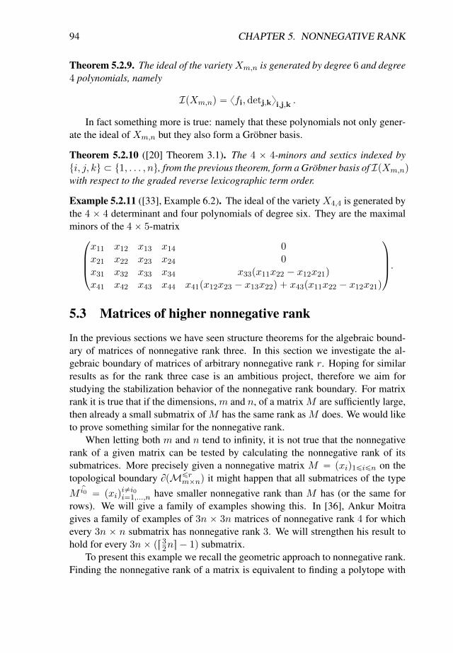
94 CHAPTER 5. NONNEGATIVE RANK
Theorem 5.2.9. The ideal of the varietyXm,n is generated by degree 6 and degree4 polynomials, namely
IpXm,nq “ xfi, detj,kyi,j,k .
In fact something more is true: namely that these polynomials not only gener-ate the ideal of Xm,n but they also form a Grobner basis.
Theorem 5.2.10 ([20] Theorem 3.1). The 4 ˆ 4-minors and sextics indexed byti, j, ku Ă t1, . . . , nu, from the previous theorem, form a Grobner basis of IpXm,nq
with respect to the graded reverse lexicographic term order.
Example 5.2.11 ([33], Example 6.2). The ideal of the varietyX4,4 is generated bythe 4 ˆ 4 determinant and four polynomials of degree six. They are the maximalminors of the 4ˆ 5-matrix
¨
˚
˚
˝
x11 x12 x13 x14 0x21 x22 x23 x24 0x31 x32 x33 x34 x33px11x22 ´ x12x21qx41 x42 x43 x44 x41px12x23 ´ x13x22q ` x43px11x22 ´ x12x21q
˛
‹
‹
‚
.
5.3 Matrices of higher nonnegative rank
In the previous sections we have seen structure theorems for the algebraic bound-ary of matrices of nonnegative rank three. In this section we investigate the al-gebraic boundary of matrices of arbitrary nonnegative rank r. Hoping for similarresults as for the rank three case is an ambitious project, therefore we aim forstudying the stabilization behavior of the nonnegative rank boundary. For matrixrank it is true that if the dimensions, m and n, of a matrix M are sufficiently large,then already a small submatrix of M has the same rank as M does. We would liketo prove something similar for the nonnegative rank.
When letting both m and n tend to infinity, it is not true that the nonnegativerank of a given matrix can be tested by calculating the nonnegative rank of itssubmatrices. More precisely given a nonnegative matrix M “ pxiq1ďiďn on thetopological boundary BpMďr
mˆnq it might happen that all submatrices of the typeM
pi0 “ pxiqi‰i0i“1,...,n have smaller nonnegative rank than M has (or the same for
rows). We will give a family of examples showing this. In [36], Ankur Moitragives a family of examples of 3n ˆ 3n matrices of nonnegative rank 4 for whichevery 3n ˆ n submatrix has nonnegative rank 3. We will strengthen his result tohold for every 3nˆ pr32ns´ 1q submatrix.
To present this example we recall the geometric approach to nonnegative rank.Finding the nonnegative rank of a matrix is equivalent to finding a polytope with
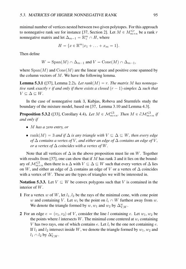
5.3. MATRICES OF HIGHER NONNEGATIVE RANK 95
minimal number of vertices nested between two given polytopes. For this approachto nonnegative rank see for instance [37, Section 2]. Let M P Mďr
mˆn be a rank rnonnegative matrix and let ∆m´1 “ Rm` XH , where
H “ tx P Rm|x1 ` . . .` xm “ 1u.
Then define
W “ SpanpMq X∆m´1 and V “ ConepMq X∆m´1,
where SpanpMq and ConepMq are the linear space and positive cone spanned bythe column vectors of M . We have the following lemma.
Lemma 5.3.1 ([37], Lemma 2.2). Let rankpMq “ r. The matrix M has nonnega-tive rank exactly r if and only if there exists a closed pr ´ 1q-simplex ∆ such thatV Ď ∆ ĎW .
In the case of nonnegative rank 3, Kubjas, Robeva and Sturmfels study theboundary of the mixture model, based on [37, Lemma 3.10 and Lemma 4.3].
Proposition 5.3.2 ([33], Corollary 4.4). Let M PMď3mˆn. Then M P BMď3
mˆn ifand only if
• M has a zero entry, or
• rankpMq “ 3 and if ∆ is any triangle with V Ď ∆ Ď W , then every edgeof ∆ contains a vertex of V , and either an edge of ∆ contains an edge of V ,or a vertex of ∆ coincides with a vertex of W .
Note that all vertices of ∆ in the above proposition must lie on W . Togetherwith results from [37], one can show that if M has rank 3 and it lies on the bound-ary ofMď3
mˆn then there is a ∆ with V Ď ∆ ĎW such that every vertex of ∆ lieson W , and either an edge of ∆ contains an edge of V or a vertex of ∆ coincideswith a vertex of W . These are the types of triangles we will be interested in.
Notation 5.3.3. Let V Ď W be convex polygons such that V is contained in theinterior of W .
1 For a vertex w of W , let l1, l2 be the rays of the minimal cone, with cone pointw and containing V . Let wi be the point on li XW furthest away from w.We denote the triangle formed by w,w1 and w2 by ∆w
V,W .
2 For an edge e “ pv1, v2q of V , consider the line l containing e. Let w1, w2 bethe points where l intersectsW . The minimal cone centered atwi containingV has two rays, one of which contains e. Let li be the one not containing e.If l1 and l2 intersect inside W , we denote the triangle formed by w1, w2 andl1 X l2 by ∆e
V,W .
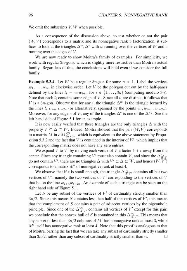
96 CHAPTER 5. NONNEGATIVE RANK
We omit the subscripts V,W when possible.
As a consequence of the discussion above, to test whether or not the pairpW,V q corresponds to a matrix and its nonnegative rank 3 factorization, it suf-fices to look at the triangles ∆w,∆e with w running over the vertices of W and erunning over the edges of V .
We are now ready to show Moitra’s family of examples. For simplicity, wework with regular 3n-gons, which is slightly more restrictive than Moitra’s actualfamily. Regardless of this, the conclusions will hold even if we consider the fullfamily.
Example 5.3.4. Let W be a regular 3n-gon for some n ą 1. Label the verticesw1, . . . , w3n in clockwise order. Let V be the polygon cut out by the half-panesdefined by the lines li “ wiwi`n for i P t1, . . . , 3nu (computing modulo 3n).Note that each li contains some edge of V . Since all li are distinct, it follows thatV is a 3n-gon. Observe that for any i, the triangle ∆wi is the triangle formed bythe lines li, li`n, li`2n (or alternatively, spanned by the points wi, wi`n, wi`2n).Moreover, for any edge e of V , any of the triangles ∆e is one of the ∆wi . See theleft hand side of Figure 5.1 for an example.
It is now easily verified that these triangles are the only triangles ∆ with theproperty V Ď ∆ Ď W . Indeed, Moitra showed that the pair pW,V q correspondsto a matrix M in BMď3
3nˆ3n, which is equivalent to the above statement by Propo-sition 5.3.2 and the fact that V is contained in the interior ofW , which implies thatthe corresponding matrix does not have any zero entries.
We expand V to V 1 by moving each vertex of V a factor 1` ε away from thecenter. Since any triangle containing V 1 must also contain V , and since the ∆wi
W,V
do not contain V 1, there are no triangles ∆ with V 1 Ď ∆ ĎW , and hence pW,V 1qcorresponds to a matrix M 1 of nonnegative rank at least 4.
We observe that if ε is small enough, the triangle ∆wiW,V 1 contains all but two
vertices of V 1, namely the two vertices of V 1 corresponding to the vertices of Vthat lie on the line wi`nwi`2n. An example of such a triangle can be seen on theright hand side of Figure 5.1.
Let S be any subset of the vertices of V 1 of cardinality strictly smaller than3n{2. Since this means S contains less than half of the vertices of V 1, this meansthat the complement of S contains a pair of adjacent vertices by the pigeonholeprinciple. Since one of the ∆wi
W,V 1 contains all vertices of V 1 except for this pair,we conclude that the convex hull of S is contained in this ∆wi
W,V 1 . This means thatany subset of less than 3n{2 columns of M 1 has nonnegative rank at most 3, whileM 1 itself has nonnegative rank at least 4. Note that this proof is analogous to thatof Moitra, barring the fact that we can take any subset of cardinality strictly smallerthan 3n{2, rather than any subset of cardinality strictly smaller than n.
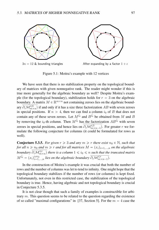
5.3. MATRICES OF HIGHER NONNEGATIVE RANK 97
3n = 12 & bounding triangles After expanding by a factor 1 + ε
Figure 5.1: Moitra’s example with 12 vertices
We have seen that there is no stabilization property on the topological bound-ary of matrices with given nonnegative rank. The reader might wonder if this istrue more generally for the algebraic boundary as well? Despite Moitra’s exam-ple (for the topological boundary), stabilization holds for r “ 3 on the algebraicboundary. A matrix M P Rmˆn not containing zeroes lies on the algebraic bound-ary BpMď3
mˆnq if and only if it has a size three factorization AB with seven zeroesin special positions. If n ą 4, then we can find a column i0 of B that does notcontain any of these seven zeroes. Let M pi0 and B pi0 be obtained from M and Bby removing the i0-th column. Then M pi0 has the factorization AB pi0 with sevenzeroes in special positions, and hence lies on BpMď3
mˆn´1q. For greater r we for-mulate the following conjecture for columns (it could be formulated for rows aswell).
Conjecture 5.3.5. For given r ě 3 and any m ě r there exist n0 P N, such thatfor all n ě n0 and m ě r and for all matrices M “ pxiqi“1,...,n on the algebraicboundary BpMďr
mˆnq there is a column 1 ď i0 ď n such that the truncated matrixM
pi0 “ pxiqi‰i0i“1,...,n lies on the algebraic boundary BpMďr
mˆn´1q.
In the construction of Moitra’s example it was crucial that both the number ofrows and the number of columns was let to tend to infinity. One might hope that thetopological boundary stabilizes if the number of rows (or columns) is kept fixed.Unfortunately, not even in this restricted case, the stabilization of the topologicalboundary is true. Hence, having algebraic and not topological boundary is crucialin Conjecture 5.3.5.
It is not clear though that such a family of examples is constructible for arbi-trary m. This question seems to be related to the question regarding the existenceof so called ”maximal configurations” in [37, Section 5]. For the m “ 4 case the
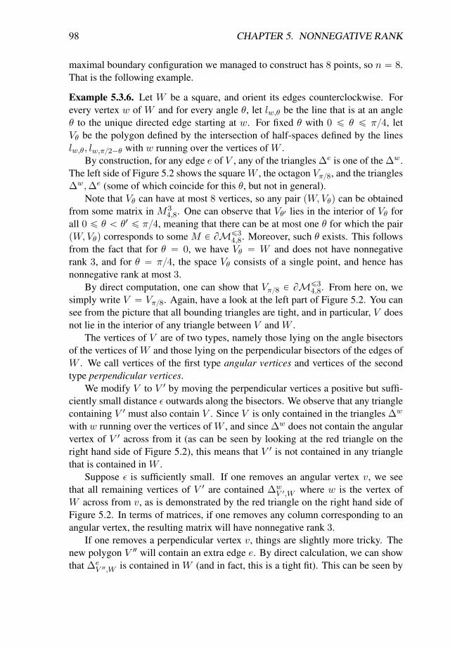
98 CHAPTER 5. NONNEGATIVE RANK
maximal boundary configuration we managed to construct has 8 points, so n “ 8.That is the following example.
Example 5.3.6. Let W be a square, and orient its edges counterclockwise. Forevery vertex w of W and for every angle θ, let lw,θ be the line that is at an angleθ to the unique directed edge starting at w. For fixed θ with 0 ď θ ď π{4, letVθ be the polygon defined by the intersection of half-spaces defined by the lineslw,θ, lw,π{2´θ with w running over the vertices of W .
By construction, for any edge e of V , any of the triangles ∆e is one of the ∆w.The left side of Figure 5.2 shows the squareW , the octagon Vπ{8, and the triangles∆w,∆e (some of which coincide for this θ, but not in general).
Note that Vθ can have at most 8 vertices, so any pair pW,Vθq can be obtainedfrom some matrix in M3
4,8. One can observe that Vθ1 lies in the interior of Vθ forall 0 ď θ ă θ1 ď π{4, meaning that there can be at most one θ for which the pairpW,Vθq corresponds to some M P BMď3
4,8. Moreover, such θ exists. This followsfrom the fact that for θ “ 0, we have Vθ “ W and does not have nonnegativerank 3, and for θ “ π{4, the space Vθ consists of a single point, and hence hasnonnegative rank at most 3.
By direct computation, one can show that Vπ{8 P BMď34,8. From here on, we
simply write V “ Vπ{8. Again, have a look at the left part of Figure 5.2. You cansee from the picture that all bounding triangles are tight, and in particular, V doesnot lie in the interior of any triangle between V and W .
The vertices of V are of two types, namely those lying on the angle bisectorsof the vertices of W and those lying on the perpendicular bisectors of the edges ofW . We call vertices of the first type angular vertices and vertices of the secondtype perpendicular vertices.
We modify V to V 1 by moving the perpendicular vertices a positive but suffi-ciently small distance ε outwards along the bisectors. We observe that any trianglecontaining V 1 must also contain V . Since V is only contained in the triangles ∆w
with w running over the vertices of W , and since ∆w does not contain the angularvertex of V 1 across from it (as can be seen by looking at the red triangle on theright hand side of Figure 5.2), this means that V 1 is not contained in any trianglethat is contained in W .
Suppose ε is sufficiently small. If one removes an angular vertex v, we seethat all remaining vertices of V 1 are contained ∆w
V 1,W where w is the vertex ofW across from v, as is demonstrated by the red triangle on the right hand side ofFigure 5.2. In terms of matrices, if one removes any column corresponding to anangular vertex, the resulting matrix will have nonnegative rank 3.
If one removes a perpendicular vertex v, things are slightly more tricky. Thenew polygon V 2 will contain an extra edge e. By direct calculation, we can showthat ∆e
V 2,W is contained in W (and in fact, this is a tight fit). This can be seen by
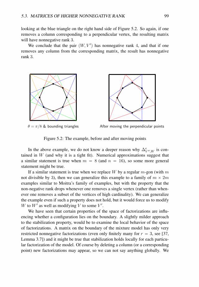
5.3. MATRICES OF HIGHER NONNEGATIVE RANK 99
looking at the blue triangle on the right hand side of Figure 5.2. So again, if oneremoves a column corresponding to a perpendicular vertex, the resulting matrixwill have nonnegative rank 3.
We conclude that the pair pW,V 1q has nonnegative rank 4, and that if oneremoves any column from the corresponding matrix, the result has nonnegativerank 3.
θ = π/8 & bounding triangles After moving the perpendicular points
Figure 5.2: The example, before and after moving points
In the above example, we do not know a deeper reason why ∆eV 2,W is con-
tained in W (and why it is a tight fit). Numerical approximations suggest thata similar statement is true when m “ 8 (and n “ 16), so some more generalstatement might be true.
If a similar statement is true when we replace W by a regular m-gon (with mnot divisible by 3), then we can generalize this example to a family of m ˆ 2mexamples similar to Moitra’s family of examples, but with the property that thenon-negative rank drops whenever one removes a single vertex (rather than when-ever one removes a subset of the vertices of high cardinality). We can generalizethe example even if such a property does not hold, but it would force us to modifyW to W 1 as well as modifying V to some V 1.
We have seen that certain properties of the space of factorizations are influ-encing whether a configuration lies on the boundary. A slightly milder approachto the stabilization property, would be to examine the local behavior of the spaceof factorizations. A matrix on the boundary of the mixture model has only veryrestricted nonnegative factorizations (even only finitely many for r “ 3, see [37,Lemma 3.7]) and it might be true that stabilization holds locally for each particu-lar factorization of the model. Of course by deleting a column (or a correspondingpoint) new factorizations may appear, so we can not say anything globally. We
100 CHAPTER 5. NONNEGATIVE RANK
formulate this idea in the following conjecture for columns (it could be formulatedfor rows as well).
Conjecture 5.3.7. For given r ě 3 and any m ě r there exists an n0 P N, suchthat for all n ě n0 and for all nonnegative factorizationsM “ AB whereM is onthe topological boundary BpMďr
mˆnq there is a column 1 ď i0 ď n and an ε ą 0such that in the ε-neighborhood of the nonnegative factorization ABi0 all size rfactorizations of M i0 are obtained from factorizations of M by removing the i0-thcolumn.
For arbitrary r we can prove this conjecture for a special case. Assume that Mlies on the topological boundary and it has a factorization such that not all verticesof the interior polytope V lie on the boundary of ∆. Let v be one such vertex.We can remove the column corresponding to v and choose ε less than the distanceof v to the closest facet of ∆. Then v does not lie on the boundary of ∆ for anysimplex ∆ in an ε neighborhood of ∆. In particular, v does not influence whether∆ contains the interior polytope V in this neighborhood, hence we can remove thisvertex.
5.4 Conclusion
In the nonnegative rank 3 case a matrix lies on the topological boundary if andonly if all nonnegative factorizations have seven zeroes in special positions (whichare isolated points in the space of factorizations, see [37, Lemma 3.7]), whereas itlies on the algebraic boundary if and only if it has at least one factorization withseven zeroes in special positions (there exists an isolated factorization). So in thenonnegative rank 3 case the above conjecture is true and it is equivalent to Conjec-ture 5.3.5. For higher r the two conjectures are not equivalent, but Conjecture 5.3.5implies Conjecture 5.3.7.
Proving any of the above conjectures would help to establish the questionwhether something similar to [33, Theorem 6.1] holds for r ą 3. Namely if itis true that for higher nonnegative rank a matrix lies on the topological (or alge-braic) boundary if and only if all (or at least one) nonnegative factorizations have(has) a given zero pattern in some special position(s).
101
Curriculum Vitae
Emil Horobet was born on December 4, 1988 in Odorheiu-Secuisesc, Roma-nia. After finishing highschool at Liceul Teoretic “Tamasi Aron” and being a silvermedalist at the International Hungarian Mathematical Contest in 2007, he studiedmathematics and computational mathematics at the “Babes-Bolyai” University inCluj-Napoca. He finished his B.Sc. and M.Sc. studies in 2010 and 2012 respec-tively. His first scientific publication appeared during his Masters’s studies, on thetopic of representation theory of skew group algebras. This publication was ex-tended and became the basis of his Masters’s thesis, which has been published asa survey book as well. He finished his studies with the highest possible grade. Be-sides attending several international conferences and workshops, he worked as anactuarial mathematician at Uniqa-Reiffeisen Software Service, Cluj-Napoca, in theperiod 2011-2012. Between 2013 and 2016 he was a research assistant at “Babes-Bolyai” University, Romania, within the project Categorical and combinatorialmethods in representation theory.
In 2012 he started his Ph.D. studies at Eindhoven University of Technology,under the supervision of Jan Draisma, within the NWO project Tensors of boundedrank. He became an active member of the international community in applied al-gebraic geometry, by participating in several conferences and by broadly interact-ing with colleagues. During this period he published five articles and three morepublications are under review. These publications are on the topics of low rankapproximations to tensors and distance minimization to algebraic varieties. Partsof these papers are presented in this dissertation. In 2016 he is selected to be oneof the six contestants for the Ph.D. prize at the BeNeLux Mathematical Congress.
102 SUMMARY
Tensors of low rank
In many applications, models of the input data involve many parameters andare naturally described by tensors. Low-rank approximation of matrices via singu-lar value decomposition is among the most important algebraic tools for solvingapproximation problems in data compression, signal processing, computer vision,etc. Low-rank approximation for tensors has the same application potential, butraises substantial mathematical challenges. One approach to this set of problemsis first to count the number of critical low-rank approximations, which we call theEuclidean distance degree to the corresponding variety of tensors.
In the introductory chapter we define the Euclidean distance degree for affineand projective varieties. Focusing mostly on varieties arising from applications,we present algebraic tools for exact computations.
The number of complex critical points of the distance function is only constantoutside a measure zero set. This exceptional set of data points where the numberof critical points differs from the generic count is called the ED discriminant. Inthe next chapter we describe the ED discriminant of affine cones.
In the next chapter we set out to count the rank-one tensors that are criticalpoints of the distance function to a general tensor. As this count depends on thegiven data tensor, we average over the space of all tensors, equipped with a Gaus-sian distribution, and find a formula that relates this average to problems in randommatrix theory. We treat both ordinary and symmetric tensors.
Unlike matrices, which always have a singular-value decomposition, higher-order tensors typically do not admit a decomposition in which the terms are pair-wise orthogonal in a strong sense. In the next chapter we prove that those orthog-onally decomposable tensors form a real-algebraic variety. In order to do this weassociate an algebra to a tensor and show that if the tensor is orthogonally decom-posable, then the algebra satisfies certain polynomial identities. Conversely, weshow that these identities imply the existence of an orthogonal decomposition.
Tensors of low rank are also important in stochastic factorization. In orderto describe the algebraic closure of the semialgebraic set of matrices of boundednonnegative rank one has to develop the theory of critical points of the dilatingfunction for the nested polytope problem. This work was done by Mond-Smith-van Straten and gave rise to the conjecture of Kubjas-Robeva-Sturmfels regardingthe algebraic boundary of matrices of nonnegative rank at most three. The finalchapter presents a proof of this conjecture.
Index
Biduality Theorem, 15
Casimir identity, 73Cayley’s cubic, 30Cayley-Menger matrix, 29conormal variety, 14critical ideal, 8
projective, 11
data isotropic locus, 28data singular locus, 21
ML, 23determinantal variety, 13dual variety, 13
Eckart-Young Theorem, 9ED correspondence, 12
joint, 15ED degree, 6
projective variety, 10average, 34
ED discriminant, 18classical, 19
essential variety, 31special, 31
evolute, 21
Hurwitz determinant, 27
Lagrange function, 7
nonnegative rank, 87algebraic boundary, 87topological boundary, 87
odeco, 58alternatingly, 59symmetrically, 59
orthogonally decomposable, 58alternatingly, 59symmetrically, 59
saturation, 8singular locus, 8
udeco, 58alternatingly, 59symmetrically, 59
unitarily decomposable, 58alternatingly, 59symmetrically, 59
103

104 INDEX
Bibliography
[1] A. Anandkumar, R. Ge, D. Hsu, S. M. Kakade, and M. Telegarski. Ten-sor decompositions for learning latent variable models. Journal of MachineLearning Research, 15:2773–2832, 2014.
[2] B. D. Anderson and U. Helmke. Counting critical formations on a line. SIAMJ. Control Optim., 52(1):219–242, 2014.
[3] B. Beauzamy, E. Bombieri, P. Enflo, and H. L. Montgomery. Products ofpolynomials in many variables. J. Number Theory, 36(2):219–245, 1990.
[4] v. F. F. Belzen and S. Weiland. Diagonalization and low-rank appromixa-tion of tensors: a singular value decomposition approach. Proceedings 18thInternational Symposium on Mathematical Theory of Networks & Systems(MTNS), 28 July - 1 August 2008, Blacksburg, Virginia, MTNS, 2008.
[5] v. F. F. Belzen and S. Weiland. Approximation of nd systems using tensordecompositions. In Multidimensional (nD) Systems, 2009. nDS 2009. Inter-national Workshop on, pages 1–8. IEEE, 2009.
[6] v. F. F. Belzen, S. Weiland, and J. De Graaf. Singular value decompositionsand low rank approximations of multi-linear functionals. In Decision andControl, 2007 46th IEEE Conference on, pages 3751–3756. IEEE, 2007.
[7] G. Blekherman, P. A. Parrilo, and R. R. Thomas, editors. Semidefinite Op-timization and Convex Algebraic Geometry. Philadelphia, PA: Society forIndustrial and Applied Mathematics (SIAM), 2013.
[8] A. Boralevi, J. Draisma, E. Horobet, and E. Robeva. Orthogonal and unitarytensor decomposition from an algebraic perspective. preprint, 2015.
[9] J. Brachat, P. Comon, B. Mourrain, and E. Tsigaridas. Symmetric tensordecomposition. Linear Algebra Appl., 433(11-12):1851–1872, 2010.
105
106 BIBLIOGRAPHY
[10] D. Cartwright and B. Sturmfels. The number of eigenvalues of a tensor.Linear Algebra Appl., 438(2):942–952, 2013.
[11] F. Catanese. Caustics of plane curves, their birationality and matrix projec-tions. In Algebraic and complex geometry. In honour of Klaus Hulek’s 60thbirthday. Based on the conference on algebraic and complex geometry, Han-nover, Germany, September 10–14, 2012, pages 109–121. Cham: Springer,2014.
[12] J. Chen and Y. Saad. On the tensor SVD and the optimal low rank orthogonalapproximation of tensors. SIAM J. Matrix Anal. Appl., 30(4):1709–1734,2009.
[13] P. Comon, G. Golub, L.-H. Lim, and B. Mourrain. Symmetric tensors andsymmetric tensor rank. SIAM J. Matrix Anal. Appl., 30(3):p1254–1279,2008.
[14] L. De Lathauwer. Decompositions of a higher-order tensor in block terms. II:Definitions and uniqueness. SIAM J. Matrix Anal. Appl., 30(3):1033–1066,2008.
[15] V. de Silva and L.-H. Lim. Tensor rank and the ill-posedness of the bestlow-rank approximation problem. SIAM J. Matrix Anal. Appl., 30(3):p1084–1127, 2008.
[16] A. Dempster, N. Laird, and D. Rubin. Maximum likelihood from incompletedata via the EM algorithm. Discussion. J. R. Stat. Soc., Ser. B, 39:1–38, 1977.
[17] J. Draisma and E. Horobet. The average number of critical rank-one approx-imations to a tensor. Linear Multilinear Algebra, to appear, 2016.
[18] J. Draisma, E. Horobet, G. Ottaviani, B. Sturmfels, and R. R. Thomas. TheEuclidean distance degree of an algebraic variety. Found. Comput. Math.,16(1):99–149, 2016.
[19] D. Drusvyatskiy, H.-L. Lee, and R. R. Thomas. Counting real critical pointsof the distance to orthogonally invariant matrix sets. SIAM Journal on MatrixAnalysis and Applications, 36(3):1360–1380, 2015.
[20] R. H. Eggermont, E. Horobet, and K. Kubjas. Algebraic boundary of matricesof nonnegative rank at most three. arXiv:1412.1654, 2014.
[21] S. Friedland and G. Ottaviani. The number of singular vector tuples anduniqueness of best rank-one approximation of tensors. Found. Comput.Math., 14(6):1209–1242, 2014.
BIBLIOGRAPHY 107
[22] I. Gelfand, M. Kapranov, and A. Zelevinsky. Discriminants, Resultants,and Multidimensional Determinants. Boston, MA: Birkhauser, reprint ofthe 1994 edition, 2008.
[23] D. R. Grayson and M. E. Stillman. Macaulay 2, a software system for re-search in algebraic geometry, 2002.
[24] R. Hartley and A. Zisserman. Multiple View Geometry in Computer Vision.Cambridge: Cambridge University Press, 2000.
[25] C. Hillar and L.-H. Lim. Most tensor problems are NP hard. Journal of theACM, 60(6):Art. 45, 2013.
[26] H. Hopf. Ein toplogischer Beitrag zur reellen Algebra. volume 13, pages219–239. Springer, 1940.
[27] E. Horobet. The data singular and the data isotropic loci for affine cones.Comm. Algebra, to appear, 2016.
[28] E. Horobet and J. I. Rodriguez. The maximum likelihood data singular locus.J. Symbolic Comput., under revision, 2016.
[29] N. Ilyushechkin. Discriminant of the characteristic polynomial of a normalmatrix. Math. Notes, 51(3):1, 1992.
[30] A. Josse and F. Pene. On the degree of caustics by reflection. Commun.Algebra, 42(6):2442–2475, 2014.
[31] A. W. Knapp. Lie Groups Beyond an Introduction. 2nd ed. Boston, MA:Birkhauser, 2nd ed. edition, 2002.
[32] T. G. Kolda. Orthogonal tensor decompositions. SIAM J. Matrix Anal. Appl.,23(1):243–255, 2001.
[33] K. Kubjas, E. Robeva, and B. Sturmfels. Fixed points of the EM algorithmand nonnegative rank boundaries. Ann. Stat., 43(1):422–461, 2015.
[34] M. Laurent and S. Poljak. On the facial structure of the set of correlationmatrices. SIAM J. Matrix Anal. Appl., 17(3):530–547, 1996.
[35] M. Michałek, B. Sturmfels, C. Uhler, and P. Zwiernik. Exponential varieties.Proc. London Math. Soc., 2016.
[36] A. Moitra. An almost optimal algorithm for computing nonnegative rank.In Proceedings of the Twenty-Fourth Annual ACM-SIAM Symposium on Dis-crete Algorithms, pages 1454–1464. SIAM, 2013.
108 BIBLIOGRAPHY
[37] D. Mond, J. Q. Smith, and D. van Straten. Stochastic factorizations, sand-wiched simplices and the topology of the space of explanations. Proc. R. Soc.Lond., Ser. A, Math. Phys. Eng. Sci., 459(2039):2821–2845, 2003.
[38] R. J. Muirhead. Aspects of Multivariate Statistical Theory. Wiley Series inProbability and Mathematical Statistics. New York: John Wiley & Sons, Inc.XIX, 673 p. (1982).
[39] M. Nagata. Remarks on a paper of Zariski on the purity of branch loci. Proc.Natl. Acad. Sci. USA, 44:796–799, 1958.
[40] L. Pachter and B. Sturmfels. Algebraic Statistics for Computational Biology.Cambridge University Press, 2005.
[41] P. A. Parrilo. Structured Semidefinite Programs and Semialgebraic GeometryMethods in Robustness and Optimization. PhD thesis, Caltech, Pasadena,CA, 2000.
[42] C. Procesi. Lie Groups. An Approach through Invariants and Representa-tions. New York, NY: Springer, 2007.
[43] E. Robeva. Orthogonal decomposition of symmetric tensors.arXiv:1409.6685, 2014.
[44] A. Rouault. Asymptotic behavior of random determinants in the Laguerre,Gram and Jacobi ensembles. ALEA, Lat. Am. J. Probab. Math. Stat., 3:181–230, 2007.
[45] G. Salmon. A Treatise on the Higher Plane Curves. 1879. http://archive.org/details/117724690.
[46] B. Sturmfels. Solving Systems of Polynomial Equations. Providence, RI:American Mathematical Society (AMS), 2002.
[47] T. Tao and V. Vu. A central limit theorem for the determinant of a Wignermatrix. Adv. Math., 231(1):74–101, 2012.
[48] J. B. Thomassen, P. H. Johansen, and T. Dokken. Closest points, moving sur-faces, and algebraic geometry. In Mathematical methods for curves and sur-faces: Tromsø 2004. Sixth international conference on mathematical methodsfor curves and surfaces, celebrating the 60th birthday of Tom Lyche, Tromsø,Norway, July 1–6, 2004., pages 351–362. Brentwood, TN: Nashboro Press,2005.

BIBLIOGRAPHY 109
[49] C. Trifogli. Focal loci of algebraic hypersurfaces: a general theory. Geome-triae Dedicata, 70(1):1–26, 1998.
[50] O. Zariski. On the purity of the branch locus of algebraic functions. Proc.Natl. Acad. Sci. USA, 44:791–796, 1958.
[51] T. Zhang and G. H. Golub. Rank-one approximation to high order tensors.SIAM J. Matrix Anal. Appl., 23(2):534–550, 2001.