Embed Size (px)
Citation preview
NASA Technical Paper 3468ARL Technical Report 480
Ten-Year Ground Exposure of CompositeMaterials Used on the Bell Model 206LHelicopter Flight Service Program
Donald J. Baker
September 1994

NASA Technical Paper 3468ARL Technical Report 480
Ten-Year Ground Exposure of CompositeMaterials Used on the Bell Model 206LHelicopter Flight Service ProgramDonald J. BakerVehicle Structures DirectorateU.S. Army Research LaboratoryLangley Research Center � Hampton, Virginia
National Aeronautics and Space AdministrationLangley Research Center � Hampton, Virginia 23681-0001
September 1994

The use of trademarks or names of manufacturers in this
report is for accurate reporting and does not constitute an
o�cial endorsement, either expressed or implied, of suchproducts or manufacturers by the National Aeronautics and
Space Administrationor by the U.S. Army Research Laboratory.
This publication is available from the following sources:
NASA Center for AeroSpace Information National Technical Information Service (NTIS)
800 Elkridge Landing Road 5285 Port Royal Road
LinthicumHeights, MD 21090-2934 Spring�eld, VA 22161-2171
(301) 621-0390 (703) 487-4650

Abstract
Residual strength results are presented for four composite materialsystems that have been exposed for up to 10 years to the environment at�ve di�erent locations on the North American Continent. The exposurelocations are near where the Bell Model 206L helicopters, which participatedin a ight service program sponsored by NASA Langley Research Centerand the U.S. Army, were ying in daily commercial service. The compositematerial systems are (1) Kevlar-49 fabric/F-185 epoxy; (2) Kevlar-49fabric/LRF-277 epoxy; (3) Kevlar-49 fabric/CE-306 epoxy; and (4) T-300graphite/E-788 epoxy. Six replicates of each material were removed andtested after 1, 3, 5, 7, and 10 years of exposure. The average baselinestrength was determined from testing six as-fabricated specimens. Morethan 1700 specimens have been tested. All specimens that were tested todetermine their strength were painted with a polyurethane paint. Each setof specimens also included an unpainted panel for observing the weatheringe�ects on the composite materials. A statistically based procedure has beenused to determine the strength value above which at least 90 percent ofthe population is expected to fall with a 95-percent con�dence level. Thecomputed compression strengths are 80 to 89 percent of the baseline (no-exposure) strengths. The resulting compression strengths are approximately8 percent below the population mean strengths. The computed short-beam-shear strengths are 83 to 92 percent of the baseline (no-exposure) strengths.The computed tension strength of all materials is 93 to 97 percent of thebaseline (no-exposure) strengths.
Introduction
The in uence of moisture on the long-termstrength and sti�ness of advanced composite mate-rials and aircraft components made from these ma-terials is an on-going concern of aircraft designersand manufacturers. As a result of moisture andother operational concerns, NASA Langley ResearchCenter and the U.S. Army initiated ight andground-based environmental e�ects programs to as-sess the performance of advanced composite mate-rials and structures subjected to normal operatingenvironments. Primary and secondary structuralcomponents have been in service on transport air-craft since the early 1970's. The �rst major heli-copter ight service program, initiated in 1978, in-cluded the installation of three Kevlar-491/epoxycomponents and one graphite/epoxy component onthe Bell Model 206L helicopter. These componentswere Federal Aviation Administration (FAA) certi-�ed and own in commercial service. Because mosthelicopters spend a considerable portion of their ser-vice life on or near the ground, a series of coupontests were performed to assess the long-term e�ects
1Kevlar-49 is a registered trademark of E. I. du Pont
de Nemours & Co., Inc.
of ground-based environments on the composite ma-terials used on the Bell Model 206L components.The locations selected for the ground-based speci-men exposure sites are in the general areas where thecomposite components are being own in service.
This paper presents a summary of residualstrength test results of all specimens that have beenexposed for up to 10 years. Detailed test results forspecimens that have been exposed for 7 and 10 yearsare included in the appendix. Detailed results forspecimens exposed for the �rst 5 years of the 10-yearprogram are presented in reference 1.
Exposure Specimens
Coupon specimens have been exposed at �ve lo-cations on the North American Continent, as shownin �gure 1. The selected areas include a hot, humid,salt-spray environment (Cameron, Louisiana, and ano�shore oil platform in the Gulf of Mexico), a coldenvironment (Fort Greely, Alaska); a cold, damp,pollution-prone environment (Toronto, Canada); anda mild, humid environment (Hampton, Virginia).The selected locations are in the general areas wherehelicopters with the composite components are be-ing own in service. Each location contains onerack, as shown in �gure 2. The racks were installed

in 1980, and each rack contains �ve trays of speci-mens. A tray of specimens contains 24 each of ten-sion, short-beam-shear (SBS) and Illinois Instituteof Technology Research Institute (IITRI) compres-sion specimens and four 2.0-in-wide specimens toprovide information on weathering characteristics ofeach material system. The tension, compression, andSBS specimens were painted with a polyurethanepaint (IMIRON2) that is used on the ight ser-vice helicopters. Specimen geometry is given inreference 1.
The four composite material systems in theground exposure program are as follows:(1) Kevlar-49 fabric (style 281)/F-1853 epoxy[0f=45f=0f ]s; (2) Kevlar-49 fabric (style 120)/
LRF-2774 epoxy [0f=90f=�45f ]s; (3) Kevlar-49
fabric (style 281)/CE-3065 epoxy [0f=90f ]s; and
(4) T-300 graphite6/E-7887 epoxy [0=�45=0]s. TheF-185 and the LRF-277 are 250�F cure epoxy sys-tems. The CE-306 is a 250�F cure epoxy system thatwas cured at 200�F for 5 hr for this application. TheE-788 is a 350�F cure epoxy. Style 281 Kevlar-49fabric, which is a plain weave fabric with 17 ends/in.of 1140 denier yarn in each direction, has a weightof 5.0 oz/yd2. Style 120 Kevlar-49 fabric, which isa plain weave fabric with 34 ends/in. of 195 denieryarn in each direction, has a weight of 1.8 oz/yd2.
The specimens used for moisture determinationwere cut from the tested tension specimens. A0.5-in-long section was cut from the undamaged areaof the tension specimens as soon as possible aftertest completion. The paint was removed by sanding,using caution not to remove an excessive amount ofthe outer ply. Each specimen was weighed after thepaint was removed. A 0.5-in-long specimen was alsoremoved from the unpainted exposure specimens andweighed prior to being used for moisture determina-tion. All specimens were stored in sealed plastic bagsbetween di�erent operations.
Test Methods
Each tray of specimens was in a sealed plas-tic bag when it was received at NASA Langley
2IMIRON is a trademark of E. I. du Pont de Nemours &
Co., Inc.
3F-185 is manufactured by Hexcel Corporation.
4LRF-277 is manufactured by Brunswick Corporation.
5CE-306 is manufactured by Ferro Corporation.
6T-300 is manufactured by Ammoco Performance
Products, Inc.
7E-788 is manufactured by U.S. Polymetric Company.
Research Center. The trays remained in the sealedbag until testing was initiated. All tests were per-formed at room temperature on six replicates foreach specimen type. The tests were performed inaccordance with the following American Society forTesting and Materials (ASTM) standards (ref. 2):(1) Tension{D3039-(76); (2) SBS{D2344-(76); and(3) Compression{D3410-(75) using the IITRI test�xture.
The specimens used for moisture determinationwere placed in a vacuum oven at 140�F. Each spec-imen was weighed periodically to determine weightloss as a function of drying time.
Data Analysis
Statistically based mechanical properties havebeen de�ned for each of the materials used inthis environmental exposure program. A proce-dure for determining statistically based mechani-cal properties for composite materials is detailed inMIL-HDBK-17-1C (ref. 3). The material used in theexposure program will not meet all the requirementsof MIL-HDBK-17-1C because a minimum of �ve lotsof material were required in the data sample, and ini-tial material inspection requirements were added tothe handbook after this environmental exposure pro-gram was initiated. Although all the requirementsof MIL-HDBK-17-1C cannot be maintained, a �nalmechanical property value can be determined. Atleast 90 percent of the population of values is ex-pected to exceed this �nal value with a 95-percentcon�dence interval. This �nal value is normally con-sidered the B-basis value. For this report, the B-basisvalue will be called B-value because all the require-ments in MIL-HDBK-17-1C for a B-basis value can-not be ful�lled. A step-by-step method for selectingthe appropriate computational method is outlined inMIL-HDBK-17-1C, and this method contains proce-dures that evaluate several di�erent statistical mod-els and determines which model, if any, adequatelydescribes the data. The procedures include meth-ods for detecting outliers, testing the compatibilityof several batches of data, and investigating the formof the underlying population from which a sample isdrawn.
A owchart of the statistical procedure used inthe present report is shown in �gure 3, and a step-by-step statistical procedure for data analysis is asfollows:
1. The sample data should be visually inspectedfor observations that are suspected of beingoutliers. Each sample is analyzed to deter-mine potential outliers using the maximum\normed" residual outlier test. The computed
2

statistic is compared with the critical statis-tic for the sample size at a 0.05 signi�cancelevel. If the computed statistic is greater thanthe critical value, the data are reviewed forpossible errors; otherwise, go to the next step.
2. The k-sample Anderson-Darling test is usedto test the hypothesis that the mechanicalproperty data from di�erent samples are in-dependent random samples of the same pop-ulation. The calculated test statistic is com-pared with the critical value for the samplesize at a 0.05 signi�cance level. If the teststatistic is less than the critical value, the sam-ples should be treated as a single population,and the pooled data should be checked for out-liers (step 4). If the calculated test statistic isequal to or greater than the critical value, it isconcluded that the samples are not identicallydistributed, and the equality-of-variance test(step 3) should be performed.
3. The equality-of-variance test is used to testthe hypothesis that the variances of the pop-ulations from which two or more independentrandom samples were taken are equal. Thecomputed statistic is compared with the0.95 quantile of a chi-square distribution. Ifthe test does not reject the hypothesis that thevariances are equal, then the one-way analysisof variance random e�ects method (ANOVA)should be used to compute the B-value. Ifthe test is rejected, then a currently approvedmethod for computing the B-value allowablesdoes not exist. If this occurs, the sources ofvariability should be investigated.
4. The pooled data should also be visually in-spected for observations suspected of beingoutliers. The pooled data are analyzed withthe statistical outlier procedure (step 1) usinga signi�cance level of 0.05 to identify potentialoutliers. If the test indicates that outliers mayexist, the data should be checked for possibleerrors; otherwise, go to the next step.
5. The pooled data are analyzed to determinethe best �t to several statistical distributions.These tests yield an observed signi�cance level(OSL) for each of the distributions. TheOSL measures the probability of observing anAnderson-Darling statistic as extreme as thevalue that is calculated by assuming that thegiven distribution is the correct one. The testis applied sequentially to the two-parameterWeibull, normal, and lognormal distributions.If the OSL is greater than 0.05, the distri-
bution tested should be used to compute theB-value. If none of the OSL tests exceeds 0.05,a nonparametric procedure is used to computethe B-value.
The �rst assumption for determining the statis-tically based strength is to assume that the popu-lation of data includes the baseline data and all theexposure data for each material system. Each sampleof the population is considered to be the data fromone exposure site at one exposure time. This ap-proach will give a population of 120 data points from20 samples.
Results and Discussion
The exposure racks at Hampton, Virginia,Toronto, Canada, and Ft. Greely, Alaska (�g. 1),have been exposed to ground conditions for 10 years.The exposure racks at Cameron, Louisiana, and onthe o�shore oil platform in the Gulf of Mexico wereexposed for 3 years before being lost to hurricanesin 1985. All data shown for 1 and 3 years of expo-sure are from �ve exposure sites, and data for 5, 7,and 10 years of exposure are from the three remainingsites. The paint on the specimens maintained its in-tegrity for the duration of the program. The baselinestrengths for the as-fabricated specimens are given inreference 1.
Residual Compression Strength
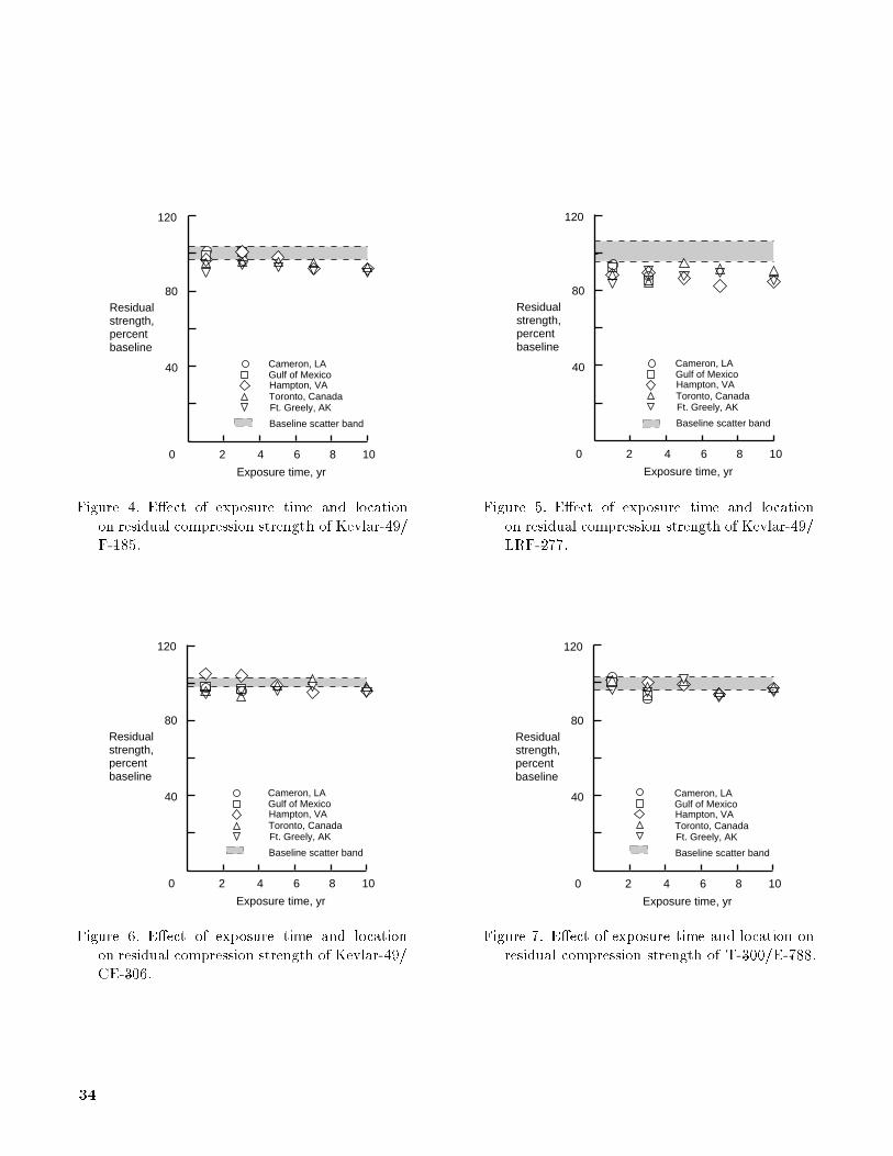
Compression tests of the composite materialswere conducted using the IITRI specimen to deter-mine the e�ect of exposure and exposure site on theresidual compression strength. The mean compres-sion failure strength and the standard deviation foreach exposure time and exposure site are given in ta-bles 1 through 4. The residual compression strengthas a function of the exposure time and the exposurelocation are presented in �gures 4 through 7. Theresidual strength shown in the �gures is the ratio ofthe mean failure stress to the mean baseline com-pressive strength for the material. Each �gure alsoshows the scatter band in baseline strength for eachmaterial.
Kevlar-49/F-185. Residual compression strengthresults for Kevlar-49/F-185 epoxy material are shownin �gure 4. The e�ects of exposure location (�g. 4) in-dicate an 11-percent variation in strength after 1 yearof exposure, a 7-percent variation after 3 years of ex-posure, and a 3-percent variation after 10 years of ex-posure. The material exposed at Ft. Greely, Alaska,had the lowest strength for all exposure times. Theaverage strength for all exposure sites indicated a3-percent loss for 1 year of exposure; this loss in-creased to an 8-percent loss for 10 years of exposure.
3

The statistical procedure just noted was applied toall the data for Kevlar-49/F-185 material tested incompression. No outliers were observed in any of the20 samples. The computed Anderson-Darling statis-tic of 2.91 exceeded the critical value of 1.28; there-fore, the sample distributions di�er signi�cantly. Thecomputed test statistic for the equality-of-variancetest is 18.88, which is less than the critical valueof 30.14. The within-samples variances are not signif-icant for the 0.05 signi�cance level; thus, the ANOVAmethod was used to compute the B-value of 17.7 ksi.This value and the minimum, maximum, and stan-dard deviation values for the population are given intable 5.
Kevlar-49/LRF-277. Residual compressionstrength results for the Kevlar-49/LRF-277 epoxymaterial are shown in �gure 5. These results indicatea 6- to 17-percent reduction in strength after 1 year ofexposure, and they also show that approximately thesame strength loss was maintained for the remainderof the exposure time. The e�ect of exposure sitelocation accounted for approximately a 10-percentdi�erence in the strength loss. After 7 years of ex-posure, the material exposed at Hampton, Virginia,had a maximum strength loss of 17 percent, whilethe material exposed at Toronto, Canada, exhibiteda minimum strength loss of 8 percent. The statisticalprocedure was applied to all the Kevlar-49/LRF-277material tested in compression. No outliers wereobserved in any of the 20 samples. The computedAnderson-Darling statistic of 2.52 exceeded the crit-ical value of 1.28; therefore, the sample distributionsdi�er signi�cantly. The computed statistic for theequality-of-variance test is 24.84, which is less thanthe critical value. Because the within-samples vari-ances are not signi�cant for the 0.05 signi�cance level,the ANOVA method was used to compute the B-value of 17.8 ksi. The B-value and the minimum,maximum, and standard deviation values for thepopulation are given in table 5.
Kevlar-49/CE-306. Residual compressionstrength results for Kevlar-49/CE-306 epoxy mate-rial are shown in �gure 6. These results indicate a2-percent loss in average strength after 1 year of ex-posure, and they show an increase to 4 percent after10 years of exposure. The e�ect of exposure loca-tion site was evident after 1 and 3 years of exposure(with the strengths varying 11 percent each). Thestatistical procedure was applied to all the materialtested in compression. One outlier was indicated ina sample of data. This outlier is within the maxi-mum, and minimum values of the total population.The computed Anderson-Darling statistic of 1.56 ex-ceeded the critical value of 1.28; therefore, the sam-
ple distributions di�er signi�cantly. The computedtest statistic for the equality-of-variance test is 18.87,which is less than the critical value of 30.14. Since thewithin-samples variances are not signi�cant for the0.05 signi�cance level, the ANOVA method was usedto compute the 16.3 ksi B-value. The B-value and theminimum, maximum, and standard deviation valuesfor the population are given in table 5.
T-300/E-788. Residual compression strengthresults for the T-300 graphite/E-788 epoxy materialare shown in �gure 7. The results do not indicateany signi�cant trends with exposure time. The aver-age residual strength loss did not exceed 6 percent.Specimens removed after 3 years of exposure indi-cated a 10-percent variance caused by exposure loca-tion, and the variance of specimens at other exposuretimes ranged from 2 to 7 percent. The statisticalprocedure was applied to all the material tested incompression. Two outliers were indicated in two dif-ferent samples. Further investigation indicated thatboth outliers were within the minimum and maxi-mum values of the total population. The computedAnderson-Darling statistic of 1.57 exceeded the crit-ical value of 1.28; therefore, the sample distributionsdi�er signi�cantly. The computed test statistic forthe equality-of-variance test is 23.04, which is lessthan the critical value of 30.14. Since the within-samples variances are not signi�cant for the 0.05 sig-ni�cance level, the ANOVA method was used tocompute the 111.0 ksi B-value. The B-value and theminimum, maximum, and standard deviation valuesfor the population are given in table 5.
The compression strengths of the exposed ma-terials have been determined by a statistical pro-cedure de�ned in MIL-HDBK-17-1C to determinethe B-value allowables of composite materials. Theresulting strengths, designated B-values, are 80to 89 percent of the baseline (no-exposure) strengths.The resulting strengths are approximately 8 percentbelow the mean strengths.
Residual Short-Beam-Shear Strength
Short-beam-shear (SBS) tests of the compositematerials were conducted to determine the e�ectsof exposure and exposure site on the residual SBSstrength. The mean SBS strength and the stan-dard deviation for each exposure time and exposuresite are given in tables 6 through 9. The resid-ual SBS strength as a function of the exposure timeand the exposure location are presented in �gures 8through 11. The residual strength shown in the �g-ures is the ratio of the mean failure stress to the meanbaseline SBS strength for the material type.
4

Kevlar-49/F-185. Residual SBS strength re-sults for Kevlar-49/F-185 epoxy material are shownin �gure 8. The e�ects of exposure location indicatea 10-percent variation in strength at 1 and 5 yearsof exposure, while the variability was 3 to 5 per-cent for the other exposure times. The average lossof strength after 10 years of exposure was 5 per-cent. No signi�cant trends were observed duringthe exposure time. The statistical procedure justnoted was applied to all the data for Kevlar-49/F-185material tested for SBS strength. Three outlierswere determined in three di�erent samples. Twoof the outliers were within the data limits for thepopulation. The other outlier determined the min-imum data value for the population, and it is ap-proximately 0.4 ksi lower than the next data value.Review of the test data did not indicate a reasonfor these data to be excluded from the population.The computed Anderson-Darling statistic of 1.92 ex-ceeded the critical value of 1.28; therefore, the sam-ple distributions di�er signi�cantly. The computedtest statistic for the equality-of-variance test is 51.28,which is greater than the critical value of 30.14.These data have failed the equality-of-variance test.The within-samples variances are signi�cant for the0.05 signi�cance level. The MIL-HDBK-17-1C cur-rently does not have an approved method for com-puting the B-value when the equality-of-variance testfails. Passing the equality-of-variance test is one ofthe assumptions required for the ANOVA method.The MIL-HDBK-17-1C suggests that the ANOVAmethod can often be applied successfully when thisassumption is not met. Using the ANOVA method,the B-value computed is 5.40 ksi, and it and the min-imum, maximum, and standard deviation values forthe population are shown in table 10. The computedvalue of 5.40 ksi is acceptable at 92 percent of thepopulation mean.
Kevlar-49/LRF-277. Residual SBS strengthresults for the Kevlar-49/LRF-277 epoxy materialare shown in �gure 9 as a function of the expo-sure time and the exposure location. The resultsshown in �gure 9 indicate a 3- to 16-percent reduc-tion in strength during the �rst 7 years of expo-sure. After 7 years of exposure, the material exposedat Hampton, Virginia, had a maximum strengthloss of 16 percent. The average strength loss wasa maximum at 12 percent after 7 years of expo-sure. The statistical procedure was applied to allof the Kevlar-49/LRF-277 material tested for SBSstrength. One outlier was observed in one of the20 samples. The outlier, which determined the mini-mum data value for the population, is 0.18 ksi lowerthan the next data value. Review of the test data
did not indicate a reason for this outlier to be ex-cluded for the population. The computed Anderson-Darling statistic of 2.40 exceeded the critical valueof 1.28; therefore, the sample distributions di�er sig-ni�cantly. The computed statistic for the equality-of-variance test is 17.96, which is less than the criticalvalue. Because the within-samples variances are notsigni�cant for the 0.05 signi�cance level, the ANOVAmethod was used to compute the B-value of 3.21 ksi.The B-value and the minimum, maximum, and stan-dard deviation values for the population are given intable 10.
Kevlar-49/CE-306. Residual SBS strength re-sults for Kevlar-49/CE-306 epoxy material are shownin �gure 10 as a function of the exposure time andthe exposure location. The specimens for 10 yearsof exposure at Ft. Greely, Alaska, were not returnedwith the tray of specimens and could not be located.Therefore, this data set contains only 19 samples and114 specimens. The data indicate an 11-percent vari-ation caused by exposure location for 1, 3, and 7 yearsof exposure. No signi�cant trends are evident andmost of the data fell within the scatter band for thebaseline specimens. The statistical procedure wasapplied to all of the material tested for SBS strength.No outliers were indicated in 19 samples of data.The computed Anderson-Darling statistic of 1.54 ex-ceeded the critical value of 1.29; therefore, the sam-ple distributions di�er signi�cantly. The computedtest statistic for the equality-of-variance test is 14.42,which is less than the critical value of 28.87. Since thewithin-samples variances are not signi�cant at the0.05 signi�cance level, the ANOVA method was usedto compute the 4.68 ksi B-value. The B-value andthe minimum, maximum, and standard deviation forthe population are given in table 10.
T-300/E-788. Residual SBS strength resultsfor the T-300/E-788 graphite/epoxy material areshown in �gure 11 as a function of the exposuretime and the exposure location. The results donot indicate any signi�cant trends with the exposuretime or the exposure location. The average residualstrength is equal to or exceeds the baseline averagestrength. The variation caused by location is be-tween 5 and 10 percent. The statistical procedurewas applied to all the T-300/E-788 material testedfor SBS strength. Two outliers were indicated in twodi�erent samples. Further investigation indicatedthat both outliers were within the minimum andmaximum values of the total population. The com-puted Anderson-Darling statistic of 1.35 exceededthe critical value of 1.28; therefore, the sample distri-butions di�er signi�cantly. The computed test statis-tic for the equality-of-variance test is 30.49, which is
5

greater than the critical value of 30.14. These datahave failed the equality-of-variance test; therefore,the within-samples variances are signi�cant for the0.05 signi�cance level. The MIL-HDBK-17-1C doesnot currently have an approved method for comput-ing the B-value when the equality-of-variance testfails. Passing the equality-of-variance test is one ofthe assumptions required for the ANOVA method.The MIL-HDBK-17-1C suggests that the ANOVAmethod can often be applied successfully when thisassumption is not met. Using the ANOVA method,the B-value computed is 10.3 ksi, and it is shown intable 10 with the minimum, maximum, and standarddeviation values for the population. The computedB-value of 10.3 ksi is acceptable at 88 percent of thepopulation mean.
The SBS strengths of the exposed materialshave been determined by a statistical procedure de-�ned in MIL-HDBK-17-1C to determine the B-valueallowables of composite materials. The resultingstrengths, designated B-values, are 83 to 92 percentof the baseline (no-exposure) strengths. The result-ing strengths are 8 to 10 percent below the meanstrengths.
Residual Tension Strength
Tension tests were conducted on the compositematerials to determine the e�ect of exposure timeand exposure site on the residual tension strength.The mean tension strength and the standard devi-ation for each exposure time and exposure site aregiven in tables 11 through 14. The e�ect of expo-sure location and the exposure time on the residualtension strength of each material is presented in �g-ures 12 through 15. Each �gure also includes thescatter band for the specimens tested to determinethe baseline strength. The residual strength shownin the �gures is the ratio of the mean failure stress tothe mean baseline tension strength for the materialtype.
Kevlar-49/F-185. Residual tension strengthresults for Kevlar-49/F-185 epoxy are shown in �g-ure 12. All the average strengths of the exposedspecimens are within the baseline scatter band. Nosigni�cant trends were observed during the expo-sure time. The statistical procedure noted abovewas applied to all the data for Kevlar-49/F-185material tested in tension. Four outliers were de-termined in three di�erent samples. Two of theoutliers were within the data limits for the popu-lation. The other outliers were the minimum andthe next lowest value for the population. Reviewof the test data did not indicate a reason for these
data to be excluded from the population. The com-puted Anderson-Darling statistic of 1.67 exceededthe critical value of 1.28; therefore, the sample dis-tributions di�er signi�cantly. The computed teststatistic for the equality-of-variance test is 65.95,which is greater than the critical value of 30.14.These data have failed the equality-of-variance test.The within-samples variances are signi�cant for the0.05 signi�cance level. The MIL-HDBK-17-1C doesnot currently have an approved method for comput-ing the B-value when the equality-of-variance testfails. Passing the equality-of-variance test is one ofthe assumptions required for the ANOVA method.The MIL-HDBK-17-1C suggests that the ANOVAmethod can often be applied successfully when thisassumption is not met. Using the ANOVA method,the B-value computed is 55.5 ksi, and it and the min-imum, maximum, and standard deviation values forthe population are shown in table 15. The computedvalue of 55.5 ksi is acceptable at 94 percent of thepopulation mean.
Kevlar-49/LRF-277. Residual tension strengthresults for the Kevlar-49/LRF-277 epoxy materialare shown in �gure 13 as a function of the ex-posure time and the exposure location. No sig-ni�cant trends were observed during the exposuretime. The statistical procedure was applied to allthe Kevlar-49/LRF-277 material. One outlier wasobserved in one of the 20 samples. The outlier waswithin the maximum and the minimum of the popu-lation. Review of the test data did not indicate a rea-son for this outlier to be excluded for this population.The computed Anderson-Darling statistic of 1.12 isless than the critical value of 1.28; therefore, the testis not signi�cant for the 0.05 level. The batch distri-butions are not signi�cantly di�erent, and the sam-ples should be treated as a single sample. Two out-liers were indicated in the pooled data. These outliersare the two lowest values in the pooled data. Reviewof the pooled data does not indicate a reason thatthese two points should be excluded from the pop-ulation. The goodness-of-�t test of the pooled datafor the two-parameter Weibull distribution yieldedan OSL of 0.839. The computed B-value from thetwo-parameter Weibull distribution is 79.1 ksi. TheB-value and the minimum, maximum, and stan-dard deviation values for the population are given intable 15.
Kevlar-49/CE-306. Residual tension strengthresults for Kevlar-49/CE-306 epoxy are shown in �g-ure 14 as a function of the exposure time and theexposure location. No signi�cant trends are evident,and all the average strengths for the exposed spec-imens fall within the scatter band for the baseline
6

specimens. The statistical procedure was appliedto all the Kevlar-49/CE-306 material tested in ten-sion. One outlier was indicated in the 20 sam-ples of data. This outlier is within the boundsof the total population of data. The computedAnderson-Darling statistic of 1.45 exceeded the crit-ical value of 1.28; therefore, the sample distribu-tions di�er signi�cantly. The computed test statis-tic for the equality of variance is 30.51, which isgreater than the critical value of 30.14. These datahave failed the equality-of-variance test; therefore,the within-samples variances are signi�cant for the0.05 signi�cance level. Using the ANOVA method,as recommended by MIL-HDBK-17-1C, the B-valuecomputed is 58.9 ksi, and it and the minimum, max-imum, and standard deviation values for the popula-tion are shown in table 15. The computed value of58.9 ksi is acceptable at 95 percent of the populationmean.
T-300/E-788. Residual tension strength re-sults for the T-300/E-788 graphite/epoxy materialare shown in �gure 15 as a function of the expo-sure time and the exposure location. The resultsdo not indicate any signi�cant trends with exposuretime. The average residual strength is equal to orexceeds the baseline average strength. The statisti-cal procedure was applied to all of the T-300/E-788material tested in tension. One outlier was indi-cated in one sample. Further investigation indicatedthat the outlier was within the minimum and maxi-mum values of the total population. The computedAnderson-Darling statistic of 1.74 exceeded the crit-ical value of 1.28; therefore, the sample distribu-tions di�er signi�cantly. The computed test statis-tic for the equality of variance is 30.96, which isgreater than the critical value of 30.14. These datahave failed the equality-of-variance test; therefore,the within-samples variances are signi�cant for the0.05 signi�cance level. Using the ANOVA method,as recommended by MIL-HDBK-17-1C, the B-valuecomputed is 117 ksi, and it and the minimum, maxi-mum, and standard deviation values for the popula-tion are shown in table 15. The computed value of117 ksi is acceptable at 91 percent of the populationmean.
The tensile strengths of the exposed materialshave been determined by a statistical procedure de-�ned in MIL-HDBK-17-1C to determine the B-valueallowables of composite materials. The resultingstrengths, designated B-values, are 93 to 97 percentof the baseline (no-exposure) strengths. The result-ing residual strengths are 6 to 9 percent below themean strengths.
Moisture Absorption
The amount of moisture that composite materialsabsorb is a function of matrix and �ber type, tem-perature, relative humidity, and exposure conditions.The objective of these tests is to determine the mois-ture absorption of composite materials when exposedto various outdoor real-time environments. A sum-mary of moisture absorption as a fraction of the com-posite specimen weight for painted specimens thatwere exposed for 3 to 10 years is tabulated in table 16and shown in �gures 16 through 19. Each data pointfor the painted specimens (open symbols) shown inthe �gures is the average of six replicates. A solid lineconnects the average moisture absorption data pointsfor each set of data. Kevlar/epoxy materials absorbfour to �ve times more moisture than graphite/epoxymaterials because the Kevlar �bers absorb moisture.The cause for the reduction in moisture absorptionat the tenth year is not evident. A number of rea-sons could cause the reduction in moisture absorp-tion, such as drought for a few months prior to re-moval and improper handling in the drying process.In general, the average values of moisture absorptioncompare well with published values for moisture ab-sorption by other Kevlar/epoxy and graphite/epoxymaterial systems (ref. 4).
A summary of the moisture absorption for un-painted material specimens is given in table 17 andshown in �gures 16 through 19. Each data point(�lled symbol) for the unpainted material is froma single specimen. A dashed line connects the av-erage moisture absorption data points for the un-painted specimens for each exposure time. TheKevlar-49/F-185 material absorbs approximately0.5 percent more moisture when painted. Paint onthe other Kevlar-49 material systems does not havea signi�cant e�ect on the moisture absorption. Thepainted T-300/E-788 graphite/epoxy material ab-sorbs approximately 0.1 percent more moisture thanthe unpainted system.
Weathering
The e�ects of weathering on bare composite spec-imens that were exposed at Hampton, Virginia, areshown in �gures 20 through 23. Each �gure showsthe as-fabricated, 1-year, 3-year, 5-year, 7-year, and10-year exposed specimens. The photographs shownin these �gures are a 15X magni�cation of the ex-posed surface. The as-fabricated and 1-year expo-sure views for Kevlar-49/F-185 material shown in �g-ure 20 indicate that the surface �bers are coated withresin. Some resin has been lost during the 1 year
7

of exposure, as noted by the reduced de�nition ofthe peel ply pattern. The 3-year exposure view hasparts of the surface ply yarns exposed because of theweathering of the surface layer epoxy. Epoxy stillremains in the valleys between the yarn crimps. Af-ter 5 years of exposure, all resin has been washedfrom the surface, and some �ber damage is evident.More damage of the surface is shown after 7 yearsof exposure. After 10 years of exposure, only frag-ments of the surface ply remain, and degradationof the second ply, a 45� ply, has started. The as-fabricated view (�g. 21) of the Kevlar-49/LRF-277material indicates that some voids are present in thesurface ply. The 1-year exposure view shows thatmost of the surface resin has been washed away andthat a few �bers are exposed. After 3 years, all theresin has been washed from between the yarns, asshown in �gure 21. Exposure for 5 through 10 yearscaused loss of the outer ply and considerable damageto the second ply. The Kevlar-49/CE-306 materialis shown in �gure 22. The photograph of the spec-imen after 1 year of exposure indicates that someresin has been washed away by the reduced de�ni-tion of the pattern of the peel ply used in fabrica-tion. Additional resin is lost after 3 years of expo-sure, thus exposing the crimped �bers as shown in�gure 22. After 5 years of exposure, only small pock-ets of resin remain in the lowest areas. Resin is alsowashed from the surface of the yarns. After 7 yearsof exposure, all resin has been washed from the ex-posed surface, and some of the yarns are starting tofray. After 10 years of exposure, the �ll yarns arelost from the near surface, some of the �bers fromthe warp yarns appear to be missing, and additionalresin is also washed from between the yarns. Viewsof T-300/E-788 graphite/epoxy material are shownin �gure 23. By the third year, the de�nition of thepeel ply has washed away. Each succeeding expo-sure time through 10 years has an increasing num-ber of bare surface �bers. The specimens exposedat the other locations have similar surface degrada-tion. This surface degradation emphasizes the needto keep composite materials protected from elementsof the environment (such as sun and rain).
Concluding Remarks
The in uence of ground-based environments onthe long-term durability of three Kevlar/epoxy sys-tems and one graphite/epoxy system has been stud-ied. Results after 10 years of ground exposureindicate that all materials exhibit good strengthretention.
A statistically based procedure has been used todetermine the strength value above which at least90 percent of the population is expected to fall witha 95-percent con�dence level. The resulting residualstrength results are summarized as follows:
1. Compression strengths are 80 to 89 percent ofthe baseline (no-exposure) strengths.
2. The resulting residual strengths are approxi-mately 8 percent below the population meanstrengths.
3. Short-beam-shear strengths are 83 to 92 per-cent of the baseline (no-exposure) strengths.The resulting residual strengths are 8 to10 percent below the mean strengths.
4. Tensile strengths are 93 to 97 percent of thebaseline (no-exposure) strengths. The result-ing residual strengths are 6 to 9 percent belowthe mean strengths.
The Kevlar-49/F-185 material absorbs approxi-mately 0.5 percent more moisture when it is painted.Paint on the other Kevlar-49 material systems doesnot have a signi�cant e�ect on moisture absorption.The painted T-300/E-788 graphite/epoxy absorbsapproximately 0.1 percent more moisture than theunpainted system.
The exposed composite specimens demonstratethe need to protect unpainted composite materialsfrom long-term environmental exposure.
NASA Langley Research Center
Hampton, VA 23681-0001June 21, 1994
8

Appendix
Detailed Test Results for Specimens
With 7 and 10 Years of Environmental
Exposure
This appendix presents the detailed results forall specimens that have been removed after 7 and10 years of exposure. The results are from exposuresites at Hampton, Virginia, Toronto, Canada, andFt. Greely, Alaska.
Residual Strength
The residual strength tables A1 through A12in this appendix include exposure time, specimensize, failure load, and computed failure stress. Theresidual strengths for each material as a function ofexposure time for each exposure location are addedto the �gures shown in reference 1 and are providedin this appendix.
Residual Compression Strength
Compression tests were conducted on specimensthat have been exposed for 7 and 10 years to deter-mine the e�ects of exposure and exposure site on theresidual compression strength. The results of testson the exposed compression specimens are given inthe following tables and �gures: table A1 and �g-ure A1 for Kevlar-49/F-185, table A2 and �gure A2for Kevlar-49/CE-306, table A3 and �gure A3 for
Kevlar-49/LRF-277, and table A4 and �gure A4 forT-300/E-788.
Residual Short-Beam-Shear Strength
Short-beam-shear (SBS) tests were conducted onspecimens that have been exposed for 7 and 10 yearsto determine the e�ects of exposure time and expo-sure site on the residual SBS strength. The resultsof tests on the exposed SBS specimens are given inthe following tables and �gures: table A5 and �g-ure A5 for Kevlar-49/F-185, table A6 and �gure A6for Kevlar-49/CE-306, table A7 and �gure A7 forKevlar-49/LRF-277, and table A8 and �gure A8 forT-300/E-788. The 10-year exposure specimens atFt. Greely, Alaska, for the Kevlar-49/CE-306 wereapparently lost or removed from the rack at someunknown time.
Residual Tension Strength
Tension tests were conducted on specimens thathave been exposed for 7 and 10 years to determinethe e�ects of exposure time and exposure site onthe residual tensile strength. The results of testson the exposed tension specimens are given in thefollowing tables and �gures: table A9 and �gure A9for Kevlar-49/F-185, table A10 and �gure A10 forKevlar-49/CE-306, table A11 and �gure A11 forKevlar-49/LRF-277, and table A12 and �gure A12for T-300/E-788.
9

References
1. Baker, Donald J.: Five Year Ground Exposure of Compos-
ite Materials Used on the Bell Model 206L Flight Service
Evaluation. NASA TM-101645, AVSCOM TM-89-B-007,
1989. (Available from DTIC as AD A233 549.)
2. Space Simulation; Aerospace and Aircraft; High Modulus
Fibers and Composites. Volume 15.03 of 1992 Annual
Book of ASTM Standards,1992.
3. Military Handbook|Polymer Matrix Composites. Vol-ume 1, Guidelines. MIL-HDBK-17-1C, Feb. 28, 1992.
(Supersedes MIL-HDBK-17-1B.)
4. Dexter, H. Benson; and Baker, Donald J.: Worldwide
Flight and Ground-Based Exposure of Composite Mate-
rials. ACEE Composite Structures Technology|Review
of Selected NASA Research on Composite Materials and
Structures,NASA CP-2321, 1984, pp. 17{50.
10

Table 1. Mean Compression Failure Stress and Standard Deviation
for Painted Kevlar-49/F-185 After Environmental Exposure
Exposure Exposure Mean failure Standardlocationa time, yr stress, psi deviation, psi
GF 1 19 946 4963 20 354 257
LA 1 20 446 5423 19 333 560
VA 1 19 654 496?? 3 20 423 541?? 5 19 691 407?? 7 18 516 936?y
10 18 634 864
Can 1 19 236 459?? 3 19 308 417?? 5 19 421 575?? 7 19 198 674?y
10 18 858 571AK 1 18 137 314?? 3 18 899 438?? 5 18 714 350?? 7 18 278 481?y
10 18 242 334aLocations are GF for Gulf of Mexico, LA for Cameron, Louisiana, VA for Hampton,
Virginia, Can for Toronto, Canada, and AK for Ft. Greely, Alaska.
Table 2. Mean Compression Failure Stress and Standard Deviation
for Painted Kevlar-49/LRF-277 After Environmental Exposure
Exposure Exposure Mean failure Standardlocationa time, yr stress, psi deviation, psi
GF 1 20 810 6353 19 140 1241
LA 1 21 052 9213 19 433 827
VA 1 19 925 1082?? 3 20 051 1509?? 5 19 359 762?? 7 18 578 935?y
10 19 108 1153Can 1 19 912 520?? 3 18 931 731?? 5 21 134 481?? 7 20 498 484?y
10 20 411 540
AK 1 18 890 509?? 3 20 449 512?? 5 19 677 1234?? 7 20 193 775?y
10 19 129 559aLocations are GF for Gulf of Mexico, LA for Cameron, Louisiana, VA for Hampton,
Virginia, Can for Toronto, Canada, and AK for Ft. Greely, Alaska.
11
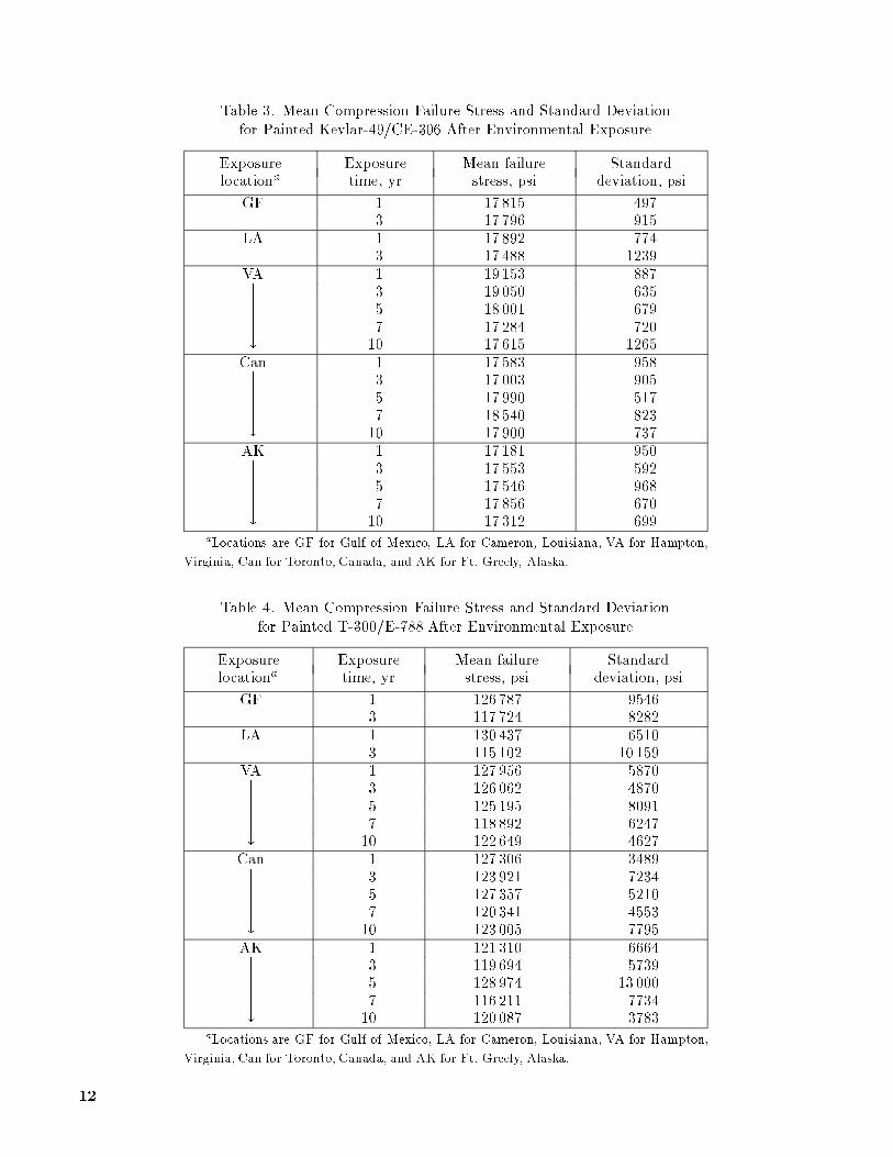
Table 3. Mean Compression Failure Stress and Standard Deviation
for Painted Kevlar-49/CE-306 After Environmental Exposure
Exposure Exposure Mean failure Standardlocationa time, yr stress, psi deviation, psi
GF 1 17 815 4973 17 796 915
LA 1 17 892 7743 17 488 1239
VA 1 19 153 887?? 3 19 050 635?? 5 18 001 679?? 7 17 284 720?y
10 17 615 1265
Can 1 17 583 958?? 3 17 003 905?? 5 17 990 517?? 7 18 540 823?y
10 17 900 737AK 1 17 181 950?? 3 17 553 592?? 5 17 546 968?? 7 17 856 670?y
10 17 312 699aLocations are GF for Gulf of Mexico, LA for Cameron, Louisiana, VA for Hampton,
Virginia, Can for Toronto, Canada, and AK for Ft. Greely, Alaska.
Table 4. Mean Compression Failure Stress and Standard Deviation
for Painted T-300/E-788 After Environmental Exposure
Exposure Exposure Mean failure Standardlocationa time, yr stress, psi deviation, psi
GF 1 126 787 95463 117 724 8282
LA 1 130 437 65103 115 102 10 159
VA 1 127 956 5870?? 3 126 062 4870?? 5 125 195 8091?? 7 118 892 6247?y
10 122 649 4627Can 1 127 306 3489?? 3 123 921 7234?? 5 127 357 5210?? 7 120 341 4553?y
10 123 005 7795
AK 1 121 310 6664?? 3 119 694 5739?? 5 128 974 13 000?? 7 116 211 7734?y
10 120 087 3783aLocations are GF for Gulf of Mexico, LA for Cameron, Louisiana, VA for Hampton,
Virginia, Can for Toronto, Canada, and AK for Ft. Greely, Alaska.
12

Table 5. Compression Strength After Environmental Exposure
[All values for properties shown are in ksi]
Material
Property Kevlar-49/F-185 Kevlar-49/LRF-277 Kevlar-49/CE-306 T-300/E-788
Mean 19.3 20.0 17.8 123Minimum 17.1 17.0 15.6 106Maximum 21.4 23.8 20.8 141Standard Deviation .878 1.22 .932 7.80B-value 17.7 17.8 16.3 111Distribution ANOVA ANOVA ANOVA ANOVA
Table 6. Mean Short-Beam-Shear Failure Stress and Standard Deviation
for Painted Kevlar-49/F-185 After Environmental Exposure
Exposure Exposure Mean failure Standardlocationa time, yr stress, psi deviation, psi
GF 1 5717 1163 6011 271
LA 1 5908 433 5992 234
VA 1 6130 134?? 3 6188 233?? 5 5923 364?? 7 5730 228?y
10 5761 308
Can 1 5789 356?? 3 5955 293?? 5 6062 172?? 7 5918 186?y
10 5610 419AK 1 5565 242?? 3 5908 210?? 5 5495 220?? 7 5975 149?y
10 5805 113aLocations are GF for Gulf of Mexico, LA for Cameron, Louisiana, VA for Hampton,
Virginia, Can for Toronto, Canada, and AK for Ft. Greely, Alaska.
13

Table 7. Mean Short-Beam-Shear Failure Stress and Standard Deviation
for Painted Kevlar-49/LRF-277 After Environmental Exposure
Exposure Exposure Mean failure Standardlocationa time, yr stress, psi deviation, psi
GF 1 3501 1093 3384 143
LA 1 3594 1093 3384 143
VA 1 3756 90?? 3 3505 86?? 5 3493 115?? 7 3241 104?y
10 3586 202
Can 1 3662 93?? 3 3496 102?? 5 3738 200?? 7 3575 145?y
10 3532 83AK 1 3395 125?? 3 3710 208?? 5 3381 94?? 7 3510 167?y
10 3566 186aLocations are GF for Gulf of Mexico, LA for Cameron, Louisiana, VA for Hampton,
Virginia, Can for Toronto, Canada, and AK for Ft. Greely, Alaska.
Table 8. Mean Short-Beam-Shear Failure Stress and Standard Deviation
for Painted Kevlar-49/CE-306 After Environmental Exposure
Exposure Exposure Mean failure Standardlocationa time, yr stress, psi deviation, psi
GF 1 5157 2293 5239 437
LA 1 5156 2363 4916 234
VA 1 5378 265?? 3 5413 265?? 5 5200 271?? 7 5436 213?y
10 5204 206Can 1 5503 314?? 3 5244 478?? 5 5041 344?? 7 4879 348?y
10 5216 189
AK 1 4892 245?? 3 5495 167?? 5 5030 224?? 7 5355 396?y
10aLocations are GF for Gulf of Mexico, LA for Cameron, Louisiana, VA for Hampton,
Virginia, Can for Toronto, Canada, and AK for Ft. Greely, Alaska.
14

Table 9. Mean Short-Beam-Shear Failure Stress and Standard Deviation
for Painted T-300/E-788 After Environmental Exposure
Exposure Exposure Mean failure Standardlocationa time, yr stress, psi deviation, psi
GF 1 11 443 6383 11 642 279
LA 1 11 320 68911 387 692
VA 1 11 412 460?? 3 11 686 505?? 5 11 562 824?? 7 11 654 882?y
10 11 431 598Can 1 11 254 708?? 3 11 968 707?? 5 11 648 936?? 7 11 789 664?y
10 11 851 756AK 1 10 389 321?? 3 11 034 702?? 5 10 772 558?? 7 11 666 416?y
10 10 822 1339aLocations are GF for Gulf of Mexico, LA for Cameron, Louisiana, VA for Hampton,
Virginia, Can for Toronto, Canada, and AK for Ft. Greely, Alaska.
Table 10. Short-Beam-Shear Strength After Environmental Exposure
[All values for properties shown are in ksi]
Material
Property Kevlar-49/F-185 Kevlar-49/LRF-277 Kevlar-49/CE-306 T-300/E-788
Mean 5.87 3.55 5.21 11.4Minimum 4.78 3.04 4.44 9.32Maximum 6.57 4.05 5.89 12.8Standard Deviation .287 .193 .328 .719B-value 5.40 3.21 4.68 10.3Distribution ANOVAa ANOVA ANOVA ANOVAaMaterial did not meet all necessary requirements.
15

Table 11. Mean Tension Failure Stress and Standard Deviation
for Painted Kevlar-49/F-185 After Environmental Exposure
Exposure Exposure Mean failure Standardlocationa time, yr stress, psi deviation, psi
GF 1 57 826 21153 59 227 1686
LA 1 58 549 16363 59 198 2357
VA 1 60 050 2798?? 3 60 773 1057?? 5 59 950 933?? 7 60 941 462?y
10 56 754 1164
Can 1 59 567 2540?? 3 60 247 1342?? 5 59 547 1250?? 7 59 187 1498?y
10 58 171 4714AK 1 58 941 5090?? 3 60 062 1309?? 5 60 732 699?? 7 60 312 1574?y
10 57 114 993aLocations are GF for Gulf of Mexico, LA for Cameron, Louisiana, VA for Hampton,
Virginia, Can for Toronto, Canada, and AK for Ft. Greely, Alaska.
Table 12. Mean Tension Failure Stress and Standard Deviation for
Painted Kevlar-49/LRF-277 After Environmental Exposure
Exposure Exposure Mean failure Standardlocationa time, yr stress, psi deviation, psi
GF 1 83 055 73263 85 719 3565
LA 1 86 507 43033 87 021 2263
VA 1 83 981 3763?? 3 86 055 6240?? 5 88 467 2078?? 7 88 057 2429?y
10 81 950 5280Can 1 86 763 2046?? 3 87 541 2870?? 5 80 579 2399?? 7 87 324 5728?y
10 86 127 3640
AK 1 85 512 5788?? 3 83 600 4974?? 5 88 894 2538?? 7 86 399 3871?y
10 85 178 3113aLocations are GF for Gulf of Mexico, LA for Cameron, Louisiana, VA for Hampton,
Virginia, Can for Toronto, Canada, and AK for Ft. Greely, Alaska.
16

Table 13. Mean Tension Failure Stress and Standard Deviation
for Painted Kevlar-49/CE-306 After Environmental Exposure
Exposure Exposure Mean failure Standardlocationa time, yr stress, psi deviation, psi
GF 1 61 382 13193 61 436 2183
LA 1 61 208 17243 60 452 1185
VA 1 63 859 1227?? 3 63 575 556?? 5 61 661 1524?? 7 63 775 1723?y
10 60 953 2824
Can 1 63 473 1580?? 3 63 770 1268?? 5 62 137 1728?? 7 61 935 2904?y
10 63 392 2028AK 1 62 668 1408?? 3 62 958 1557?? 5 60 384 2811?? 7 62 848 1554?y
10 61 767 2558aLocations are GF for Gulf of Mexico, LA for Cameron, Louisiana, VA for Hampton,
Virginia, Can for Toronto, Canada, and AK for Ft. Greely, Alaska.
Table 14. Mean Tension Failure Stress and Standard Deviation
for Painted T-300/E-788 After Environmental Exposure
Exposure Exposure Mean failure Standardlocationa time, yr stress, psi deviation, psi
GF 1 123 086 8 0123 127 850 7 676
LA 1 122 772 3 1633 127 620 8 962
VA 1 127 927 3 503?? 3 128 272 7 974?? 5 130 815 3 531?? 7 132 929 6 378?y
10 123 580 7 407Can 1 136 216 4 428?? 3 128 551 6 057?? 5 123 460 3 797?? 7 137 698 5 218?y
10 130 577 11 779
AK 1 126 887 12 586?? 3 134 628 4 375?? 5 136 193 5 601?? 7 132 673 4 134?y
10 130 005 4 942aLocations are GF for Gulf of Mexico, LA for Cameron, Louisiana, VA for Hampton,
Virginia, Can for Toronto, Canada, and AK for Ft. Greely, Alaska.
17
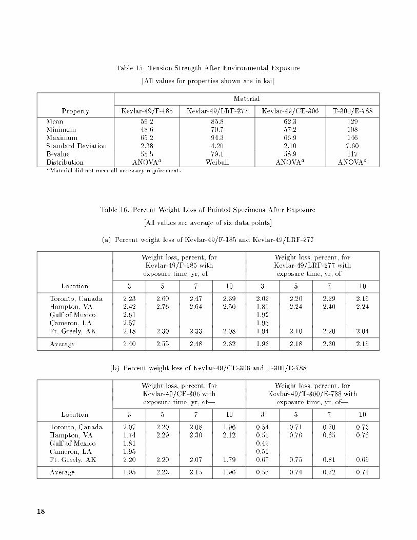
Table 15. Tension Strength After Environmental Exposure
[All values for properties shown are in ksi]
Material
Property Kevlar-49/F-185 Kevlar-49/LRF-277 Kevlar-49/CE-306 T-300/E-788
Mean 59.2 85.8 62.3 129Minimum 48.6 70.7 57.2 108Maximum 65.2 94.3 66.9 146Standard Deviation 2.38 4.20 2.10 7.60B-value 55.5 79.1 58.9 117Distribution ANOVAa Weibull ANOVAa ANOVAa
aMaterial did not meet all necessary requirements.
Table 16. Percent Weight Loss of Painted Specimens After Exposure
[All values are average of six data points]
(a) Percent weight loss of Kevlar-49/F-185 and Kevlar-49/LRF-277
Weight loss, percent, for Weight loss, percent, forKevlar-49/F-185 with Kevlar-49/LRF-277 withexposure time, yr, of| exposure time, yr, of|
Location 3 5 7 10 3 5 7 10
Toronto, Canada 2.23 2.60 2.47 2.39 2.03 2.20 2.29 2.16Hampton, VA 2.42 2.76 2.64 2.50 1.81 2.24 2.40 2.24Gulf of Mexico 2.61 1.92Cameron, LA 2.57 1.96Ft. Greely, AK 2.18 2.30 2.33 2.08 1.94 2.10 2.20 2.04
Average 2.40 2.55 2.48 2.32 1.93 2.18 2.30 2.15
(b) Percent weight loss of Kevlar-49/CE-306 and T-300/E-788
Weight loss, percent, for Weight loss, percent, forKevlar-49/CE-306 with Kevlar-49/T-300/E-788 withexposure time, yr, of| exposure time, yr, of|
Location 3 5 7 10 3 5 7 10
Toronto, Canada 2.07 2.20 2.08 1.96 0.54 0.71 0.70 0.73Hampton, VA 1.74 2.29 2.30 2.12 0.51 0.76 0.65 0.76Gulf of Mexico 1.81 0.49Cameron, LA 1.95 0.51Ft. Greely, AK 2.20 2.20 2.07 1.79 0.67 0.75 0.81 0.65
Average 1.95 2.23 2.15 1.96 0.56 0.74 0.72 0.71
18
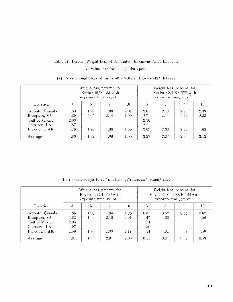
Table 17. Percent Weight Loss of Unpainted Specimens After Exposure
[All values are from single data point]
(a) Percent weight loss of Kevlar-49/F-185 and Kevlar-49/LRF-277
Weight loss, percent, for Weight loss, percent, forKevlar-49/F-185 with Kevlar-49/LRF-277 withexposure time, yr, of| exposure time, yr, of|
Location 3 5 7 10 3 5 7 10
Toronto, Canada 1.60 1.90 1.88 2.01 2.01 2.40 2.26 2.39Hampton, VA 1.69 2.05 2.14 1.99 2.71 2.11 2.44 2.33Gulf of Mexico 2.03 2.36Cameron, LA 1.87 2.11Ft. Greely, AK 1.79 1.80 1.86 1.69 2.09 2.30 2.39 1.63
Average 1.80 1.92 1.96 1.90 2.23 2.27 2.36 2.12
(b) Percent weight loss of Kevlar-49/CE-306 and T-300/E-788
Weight loss, percent, for Weight loss, percent, forKevlar-49/CE-306 with Kevlar-49/T-300/E-788 withexposure time, yr, of| exposure time, yr, of|
Location 3 5 7 10 3 5 7 10
Toronto, Canada 1.85 1.90 1.94 1.98 0.51 0.62 0.56 0.62Hampton, VA 1.62 1.96 2.10 2.01 .47 .60 .60 .56Gulf of Mexico 2.03 .74Cameron, LA 1.97 .50Ft. Greely, AK 1.59 1.70 1.99 2.17 .54 .61 .69 .58
Average 1.81 1.85 2.01 2.05 0.55 0.61 0.62 0.59
19

Table A1. Compression Strength of Painted Kevlar-49/F-185 After Environmental Exposure
(a) Specimens from exposure site at Hampton, Virginia
Specimen Exposure Width, Thickness, Failure Failurenumber time, yr in. in. load, lb stress, psi
407 7 0.2623 0.0943 455 18 395408 7 .2531 .1018 441 17 116409 7 .2634 .0972 464 18 123410 7 .2531 .0910 451 19 581411 7 .2565 .0939 471 19 555412 7 .2612 .0986 472 18 327401 10 .2535 .0961 489 20 073402 10 .2441 .0955 444 19 046403 10 .2562 .1000 450 17 564404 10 .2483 .0991 454 18 450405 10 .2563 .0982 468 18 595406 10 .2617 .1002 474 18 076
(b) Specimens from exposure site at Toronto, Canada
Specimen Exposure Width, Thickness, Failure Failurenumber time, yr in. in. load, lb stress, psi
431 7 0.2533 0.0988 465 18 581432 7 .2512 .1002 462 18 355433 7 .2479 .0962 450 18 870434 7 .2510 .0911 452 19 767435 7 .2552 .0957 484 19 818436 7 .2451 .1018 494 19 799437 10 .2493 .0936 448 19 199438 10 .2556 .0964 448 18 182439 10 .2574 .1018 475 18 127440 10 .2451 .1010 477 19 269441 10 .2547 .0944 455 18 924442 10 .2471 .1005 483 19 449
(c) Specimens from exposure site at Ft. Greely, Alaska
Specimen Exposure Width, Thickness, Failure Failurenumber time, yr in. in. load, lb stress, psi
443 7 0.2461 0.1018 457 18 241444 7 .2526 .0988 467 18 712445 7 .2578 .0996 474 18 460446 7 .2556 .0955 456 18 681447 7 .2586 .1013 456 17 407448 7 .2550 .1019 472 18 165449 10 .2404 .1001 446 18 534450 10 .2552 .0989 467 18 503451 10 .2516 .1013 452 17 734452 10 .2507 .0931 431 18 466453 10 .2576 .0987 456 17 935454 10 .2474 .1004 454 18 278
20

Table A2. Compression Strength of Painted Kevlar-49/CE-306 After Environmental Exposure
(a) Specimens from exposure site at Hampton, Virginia
Specimen Exposure Width, Thickness, Failure Failurenumber time, yr in. in. load, lb stress, psi
413F 7 0.2474 0.0972 414 17 216414F 7 .2458 .0959 421 17 860415F 7 .2574 .0981 463 18 336416F 7 .2646 .0957 413 16 310417F 7 .2691 .0955 440 17 121418F 7 .2677 .0968 437 16 864407F 10 .2579 .0986 446 17 539408F 10 .2678 .0967 405 15 639409F 10 .2551 .0964 459 18 665410F 10 .2546 .0980 473 18 957411F 10 .2497 .0997 453 18 196412F 10 .2631 .0961 422 16 690
(b) Specimens from exposure site at Toronto, Canada
Specimen Exposure Width, Thickness, Failure Failurenumber time, yr in. in. load, lb stress, psi
437F 7 0.2668 0.0831 437 19 710438F 7 .2563 .0973 442 17 724439F 7 .2662 .0957 466 18 292440F 7 .2510 .0942 457 19 328441F 7 .2467 .0931 424 18 461442F 7 .2650 .0975 458 17 726443F 10 .2477 .0973 446 18 505444F 10 .2617 .0958 414 16 513445F 10 .2674 .0955 458 17 935446F 10 .2501 .1005 449 17 864447F 10 .2563 .0958 455 18 531448F 10 .2707 .0974 476 18 053
(c) Specimens from exposure site at Ft. Greely, Alaska
Specimen Exposure Width, Thickness, Failure Failurenumber time, yr in. in. load, lb stress, psi
449F 7 0.2523 0.0967 445 18 240450F 7 .2602 .0939 444 18 172451F 7 .2387 .0982 434 18 515452F 7 .2635 .0971 425 16 611453F 7 .2470 .0952 420 17 861454F 7 .2642 .0922 432 17 735455F 10 .2660 .0951 444 17 552456F 10 .2628 .0961 414 16 393457F 10 .2549 .0952 432 17 802458F 10 .2634 .0959 419 16 587459F 10 .2598 .0952 429 17 345460F 10 .2493 .0957 434 18 191
21

Table A3. Compression Strength of Painted Kevlar-49/LRF-277 After Environmental Exposure
(a) Specimens from exposure site at Hampton, Virginia
Specimen Exposure Width, Thickness, Failure Failurenumber time, yr in. in. load, lb stress, psi
416B 7 0.2500 0.0784 354 18 061417B 7 .2207 .0776 320 18 685418B 7 .2483 .0778 368 19 050419B 7 .2277 .0767 336 19 239420B 7 .2390 .0782 364 19 476421B 7 .2621 .0765 340 16 957410B 10 .2574 .0789 367 18 071411B 10 .2565 .0781 356 17 771412B 10 .2634 .0774 382 18 737413B 10 .2328 .0759 367 20 770414B 10 .2496 .0778 389 20 032415B 10 .2333 .0772 347 19 266
(b) Specimens from exposure site at Toronto, Canada
Specimen Exposure Width, Thickness, Failure Failurenumber time, yr in. in. load, lb stress, psi
440B 7 0.2432 0.0779 402 21 219441B 7 .2302 .0764 359 20 412442B 7 .2424 .0803 408 20 961443B 7 .2368 .0782 373 20 143444B 7 .2368 .0776 372 20 244445B 7 .2577 .0766 395 20 010446B 10 .2263 .0776 347 19 760447B 10 .2229 .0786 361 20 605448B 10 .2372 .0775 370 20 127449B 10 .2301 .0788 365 20 130450B 10 .2304 .0794 390 21 319451B 10 .2505 .0780 401 20 523
(c) Specimens from exposure site at Ft. Greely, Alaska
Specimen Exposure Width, Thickness, Failure Failurenumber time, yr in. in. load, lb stress, psi
452B 7 0.2464 0.0788 396 20 395453B 7 .2356 .0778 384 20 950454B 7 .2348 .0792 384 20 649455B 7 .2510 .0779 372 19 025456B 7 .2342 .0784 357 19 443457B 7 .2425 .0781 392 20 698458B 10 .2344 .0766 337 18 769459B 10 .2465 .0771 383 20 152460B 10 .2280 .0775 341 19 298461B 10 .2520 .0769 370 19 093462B 10 .2521 .0768 360 18 594463B 10 .2553 .0793 382 18 869
22

Table A4. Compression Strength of Painted T-300/E-788 After Environmental Exposure
(a) Specimens from exposure site at Hampton, Virginia
Specimen Exposure Width, Thickness, Failure Failurenumber time, yr in. in. load, lb stress, psi
248V 7 0.2558 0.0666 2035 119 451249V 7 .2563 .0706 2130 117 714250V 7 .2558 .0693 2185 123 259251V 7 .2567 .0708 2220 122 150252V 7 .2555 .0702 1920 107 047253V 7 .2579 .0691 2205 123 731242V 10 .2559 .0714 2245 122 871243V 10 .2571 .0715 2308 125 553244V 10 .2497 .0709 2092 118 167245V 10 .2541 .0679 2010 116 499246V 10 .2513 .0677 2193 128 901247V 10 .2555 .0706 2235 123 903
(b) Specimens from exposure site at Toronto, Canada
Specimen Exposure Width, Thickness, Failure Failurenumber time, yr in. in. load, lb stress, psi
272V 7 0.2559 0.0715 2205 120 513273V 7 .2590 .0680 2015 114 411274V 7 .2667 .0681 2090 115 074275V 7 .2573 .0695 2223 124 313276V 7 .2553 .0714 2260 123 982277V 7 .2570 .0698 2220 123 755278V 10 .2559 .0717 2453 133 693279V 10 .2565 .0693 2270 127 704280V 10 .2548 .0713 2156 118 675281V 10 .2558 .0712 2178 119 585282V 10 .2554 .0695 2246 126 533283V 10 .2549 .0704 2007 111 842
(c) Specimens from exposure site at Ft. Greely, Alaska
Specimen Exposure Width, Thickness, Failure Failurenumber time, yr in. in. load, lb stress, psi
284V 7 0.2550 0.0706 1950 108 315285V 7 .2596 .0693 2165 120 343286V 7 .2570 .0685 1980 112 471287V 7 .2574 .0718 2045 110 652288V 7 .2569 .0701 2090 116 055289V 7 .2555 .0694 2295 129 429290V 10 .2571 .0660 2066 121 754291V 10 .2553 .0687 2003 114 202292V 10 .2549 .0694 2094 118 372293V 10 .2569 .0697 2164 120 854294V 10 .2513 .0676 2034 119 732295V 10 .2558 .0690 2217 125 608
23

Table A5. Short-Beam-Shear Strength of Painted Kevlar-49/F-185 After Environmental Exposure
(a) Specimens from exposure site at Hampton, Virginia
Specimen Exposure Width, Thickness, Failure Failurenumber time, yr in. in. load, lb stress, psi
91 7 0.2624 0.0941 183 555992 7 .2606 .0941 193 590393 7 .2669 .1074 206 539094 7 .2618 .0876 179 585495 7 .2603 .0953 188 568496 7 .3047 .0986 240 599185 10 .2638 .1049 197 534586 10 .2804 .1002 202 539887 10 .2609 .0938 194 595588 10 .2598 .0950 198 602089 10 .2604 .0883 184 599590 10 .2624 .0862 177 5856
(b) Specimens from exposure site at Toronto, Canada
Specimen Exposure Width, Thickness, Failure Failurenumber time, yr in. in. load, lb stress, psi
115 7 0.2568 0.0965 196 5932116 7 .2593 .0938 186 5735117 7 .2605 .0945 204 6215118 7 .2620 .0963 192 5707119 7 .2543 .1022 208 6002120 7 .2625 .0947 196 5913121 10 .2730 .0983 202 5654122 10 .2658 .1018 173 4784123 10 .2600 .0913 188 5952124 10 .2499 .0933 181 5816125 10 .2605 .0912 184 5793126 10 .2584 .1032 201 5662
(c) Specimens from exposure site at Ft. Greely, Alaska
Specimen Exposure Width, Thickness, Failure Failurenumber time, yr in. in. load, lb stress, psi
127 7 0.2485 0.0967 187 5836128 7 .2624 .0945 202 6110129 7 .2467 .0912 185 6167130 7 .2618 .0973 201 5918131 7 .2593 .0918 184 5797132 7 .2574 .0900 186 6022133 10 .2620 .0966 199 5894134 10 .2531 .0894 170 5628135 10 .2632 .0955 195 5809136 10 .2620 .0898 183 5846137 10 .2598 .0914 188 5932138 10 .2587 .1011 200 5721
24

Table A6. Short-Beam-Shear Strength of Painted Kevlar-49/CE-306 After Environmental Exposure
(a) Specimens from exposure site at Hampton, Virginia
Specimen Exposure Width, Thickness, Failure Failurenumber time, yr in. in. load, lb stress, psi
91F 7 0.2568 0.0935 177 552992F 7 .2581 .0933 171 532693F 7 .2545 .0944 172 536994F 7 .2483 .0931 176 571095F 7 .2477 .0907 153 510896F 7 .2519 .0951 178 557385F 10 .2435 .0900 152 518586F 10 .2582 .0837 147 509887F 10 .2591 .0905 159 509288F 10 .2552 .0843 143 497889F 10 .2452 .0942 171 555990F 10 .2519 .0936 167 5312
(b) Specimens from exposure site at Toronto, Canada
Specimen Exposure Width, Thickness, Failure Failurenumber time, yr in. in. load, lb stress, psi
115F 7 0.2333 0.0844 122 4647116F 7 .2488 .0877 148 5087117F 7 .2563 .0859 135 4599118F 7 .2534 .0954 174 5398119F 7 .2601 .0905 158 5034120F 7 .2287 .0822 113 4508121F 10 .2404 .0887 142 4980122F 10 .2559 .0937 173 5405123F 10 .2561 .0892 164 5394124F 10 .2574 .0864 148 4991125F 10 .2550 .0921 165 5272126F 10 .2424 .0912 155 5255
(c) Specimens from exposure site at Ft. Greely, Alaska
Specimen Exposure Width, Thickness, Failure Failurenumber time, yr in. in. load, lb stress, psi
133F 7 0.2386 0.0835 134 5044134F 7 .2570 .0930 180 5633135F 7 .2532 .0815 132 4808136F 7 .2603 .0945 191 5811137F 7 .2585 .0968 188 5638138F 7 .2400 .0852 142 5197127Fa 10 .2577 .0901128Fa 10 .2593 .0887129Fa 10 .2575 .0925130Fa 10 .2443 .0905131Fa 10 .2388 .0832132Fa 10 .2584 .0946
aSpecimens lost in service.
25

Table A7. Short-Beam-Shear Strength of Painted Kevlar-49/LRF-277 After Environmental Exposure
(a) Specimens from exposure site at Hampton, Virginia
Specimen Exposure Width, Thickness, Failure Failurenumber time, yr in. in. load, lb stress, psi
91B 7 0.2490 0.0773 85 331292B 7 .2446 .0778 84 331193B 7 .2410 .0780 82 327294B 7 .2440 .0775 82 325295B 7 .2491 .0784 85 326496B 7 .2483 .0796 80 303685B 10 .2355 .0785 92 374186B 10 .2420 .0783 98 386387B 10 .2469 .0779 94 364688B 10 .2469 .0773 87 339989B 10 .2400 .0789 84 333990B 10 .2427 .0769 88 3528
(b) Specimens from exposure site at Toronto, Canada
Specimen Exposure Width, Thickness, Failure Failurenumber time, yr in. in. load, lb stress, psi
115B 7 0.2652 0.0782 98 3544116B 7 .2451 .0781 96 3761117B 7 .2394 .0776 88 3553118B 7 .2387 .0786 86 3438119B 7 .2380 .0793 86 3418120B 7 .2507 .0777 97 3735121B 10 .2323 .0785 83 3426122B 10 .2500 .0770 94 3651123B 10 .2355 .0777 87 3562124B 10 .2480 .0770 90 3531125B 10 .2425 .0787 91 3572126B 10 .2399 .0773 85 3450
(c) Specimens from exposure site at Ft. Greely, Alaska
Specimen Exposure Width, Thickness, Failure Failurenumber time, yr in. in. load, lb stress, psi
127B 7 0.2359 0.0793 93 3729128B 7 .2387 .0781 87 3500129B 7 .2443 .0766 91 3647130B 7 .2405 .0769 87 3528131B 7 .2350 .0784 83 3379132B 7 .2310 .0803 81 3275133B 10 .2459 .0786 91 3523134B 10 .2469 .0770 98 3858135B 10 .2406 .0775 89 3580136B 10 .2380 .0775 90 3660137B 10 .2440 .0805 91 3471138B 10 .2408 .0786 83 3305
26

Table A8. Short-Beam-Shear Strength of Painted T-300/E-788 After Environmental Exposure
(a) Specimens from exposure site at Hampton, Virginia
Specimen Exposure Width, Thickness, Failure Failurenumber time, yr in. in. load, lb stress, psi
91V 7 0.2557 0.0709 307 12 70192V 7 .2557 .0710 303 12 51793V 7 .2560 .0723 255 10 33394V 7 .2572 .0729 294 11 76095V 7 .2521 .0714 275 11 45896V 7 .2563 .0732 279 11 15385V 10 .2569 .0723 265 10 68086V 10 .2568 .0724 269 10 83187V 10 .2570 .0710 290 11 91688V 10 .2558 .0729 277 11 15789V 10 .2570 .0724 280 11 27490V 10 .2537 .0720 297 12 190
(b) Specimens from exposure site at Toronto, Canada
Specimen Exposure Width, Thickness, Failure Failurenumber time, yr in. in. load, lb stress, psi
115V 7 0.2558 0.0733 284 11 360116V 7 .2557 .0720 264 10 755117V 7 .2563 .0733 303 12 096118V 7 .2562 .0730 308 12 351119V 7 .2562 .0728 290 11 661120V 7 .2570 .0709 304 12 513121V 10 .2563 .0705 275 11 402122V 10 .2564 .0741 307 12 123123V 10 .2563 .0720 315 12 802124V 10 .2582 .0732 268 10 631125V 10 .2563 .0721 303 12 281126V 10 .2573 .0737 300 11 865
(c) Specimens from exposure site at Ft. Greely, Alaska
Specimen Exposure Width, Thickness, Failure Failurenumber time, yr in. in. load, lb stress, psi
127V 7 0.2563 0.0728 293 11 777128V 7 .2578 .0729 307 12 251129V 7 .2568 .0713 293 12 002130V 7 .2545 .0723 278 11 331131V 7 .2558 .0724 283 11 461132V 7 .2570 .0721 276 11 171133V 10 .2568 .0710 227 9 317134V 10 .2568 .0721 305 12 355135V 10 .2556 .0722 282 11 477136V 10 .2564 .0721 250 10 126137V 10 .2566 .0725 236 9 518138V 10 .2574 .0735 306 12 139
27

Table A9. Tension Strength of Painted Kevlar-49/F-185 After Environmental Exposure
(a) Specimens from exposure site at Hampton, Virginia
Specimen Exposure Width, Thickness, Failure Failurenumber time, yr in. in. load, lb stress, psi
250 7 1.0015 0.0994 6100 61 276251 7 1.0015 .1005 6100 60 606252 7 1.0025 .1003 6090 60 566253 7 1.0015 .1005 6080 60 407254 7 0.9990 .1003 6150 61 377255 7 1.0030 .1000 6160 61 416244 10 1.0040 .0993 5713 57 304245 10 1.0041 .0994 5800 58 112246 10 1.0021 .0992 5501 55 337247 10 1.0010 .0992 5745 57 855248 10 1.0040 .0998 5633 56 218249 10 1.0090 .0999 5614 55 695
(b) Specimens from exposure site at Toronto, Canada
Specimen Exposure Width, Thickness, Failure Failurenumber time, yr in. in. load, lb stress, psi
274 7 1.0035 0.1000 5850 58 296275 7 1.0035 .1004 5775 57 319276 7 1.0002 .1003 6200 61 802277 7 1.0001 .1004 5950 59 257278 7 1.0045 .1005 6000 59 434279 7 0.9998 .1000 5900 59 012280 10 1.0001 .1004 5960 59 357281 10 1.0002 .1001 4898 48 921282 10 1.0006 .1008 5893 58 427283 10 1.0003 .1005 5961 59 296284 10 1.0005 .1003 6223 62 013285 10 1.0003 .1002 6115 61 010
(c) Specimens from exposure site at Ft. Greely, Alaska
Specimen Exposure Width, Thickness, Failure Failurenumber time, yr in. in. load, lb stress, psi
286 7 1.0005 0.1000 5780 57 771287 7 1.0005 .0999 6200 62 031288 7 1.0004 .1005 6000 59 678289 7 1.0004 .1002 6100 60 854290 7 1.0003 .1003 6000 59 803291 7 1.0003 .1004 6200 61 734292 10 1.0005 .0990 5741 57 961293 10 1.0001 .1004 5593 55 702294 10 1.0004 .0999 5819 58 225295 10 1.0007 .0990 5620 56 728296 10 1.0020 .1004 5673 56 391297 10 1.0007 .1003 5789 57 676
28

Table A10. Tension Strength of Painted Kevlar-49/CE-306 After Environmental Exposure
(a) Specimens from exposure site at Hampton, Virginia
Specimen Exposure Width, Thickness, Failure Failurenumber time, yr in. in. load, lb stress, psi
247F 7 0.9915 0.0923 6080 66 437248F 7 .9908 .0978 6210 64 087249F 7 .9891 .0913 5550 61 459250F 7 .9848 .0921 5740 63 286251F 7 .9923 .0961 6170 64 702252F 7 .9961 .0985 6150 62 681241F 10 .9960 .0982 5942 60 752242F 10 .9864 .0980 5528 57 186243F 10 .9870 .0913 5937 65 884244F 10 .9944 .0981 5836 59 825245F 10 .9938 .0971 5902 61 162246F 10 .9733 .0905 5365 60 908
(b) Specimens from exposure site at Toronto, Canada
Specimen Exposure Width, Thickness, Failure Failurenumber time, yr in. in. load, lb stress, psi
271F 7 0.9964 0.0994 6050 61 085272F 7 .9942 .1000 6200 62 362273F 7 .9934 .1008 5775 57 672274F 7 .9946 .0991 6575 66 707275F 7 .9993 .0980 6100 62 288276F 7 .9989 .0989 6075 61 493277F 10 .9842 .0987 6095 62 744278F 10 .9866 .0970 6407 66 949279F 10 .9780 .0918 5643 62 853280F 10 .9867 .0980 6089 62 970281F 10 .9937 .0990 6298 64 019282F 10 .9884 .0976 5867 60 818
(c) Specimens from exposure site at Ft. Greely, Alaska
Specimen Exposure Width, Thickness, Failure Failurenumber time, yr in. in. load, lb stress, psi
283F 7 0.9891 0.0962 5850 61 481284F 7 .9906 .0982 6100 62 708285F 7 .9904 .0995 6300 63 930286F 7 .9875 .1014 6100 60 919287F 7 .9923 .0990 6400 65 148288F 7 .9906 .0979 6100 62 900289F 10 .9861 .0901 5922 66 653290F 10 .9912 .0966 5798 60 554291F 10 .9931 .0864 5208 60 697292F 10 1.0061 .0977 5839 59 402293F 10 .9896 .0974 5889 61 097294F 10 .9923 .0989 6104 62 198
29

Table A11. Tension Strength of Painted Kevlar-49/LRF-277 After Environmental Exposure
(a) Specimens from exposure site at Hampton, Virginia
Specimen Exposure Width, Thickness, Failure Failurenumber time, yr in. in. load, lb stress, psi
247B 7 0.9852 0.0874 7710 89 540248B 7 .9908 .0886 7600 86 575249B 7 .9815 .0886 7610 87 511250B 7 .9904 .0872 7310 84 643251B 7 1.0049 .0887 7880 88 406252B 7 .9832 .0871 7850 91 666241B 10 .9888 .0884 6250 71 502242B 10 1.0007 .0851 7336 86 144243B 10 .9836 .0895 7231 82 140244B 10 .9927 .0868 7232 83 931245B 10 .9829 .0866 7112 83 553246B 10 .9828 .0847 7028 84 427
(b) Specimens from exposure site at Toronto, Canada
Specimen Exposure Width, Thickness, Failure Failurenumber time, yr in. in. load, lb stress, psi
271B 7 0.9948 0.0877 8075 92 557272B 7 .9878 .0878 7825 90 224273B 7 .9785 .0862 6950 82 398274B 7 .9914 .0876 7025 80 890275B 7 .9948 .0884 7350 83 579276B 7 .9886 .0885 8250 94 295277B 10 .9975 .0874 7185 82 414278B 10 1.0049 .0897 7488 83 071279B 10 .9850 .0854 7526 89 468280B 10 .9753 .0875 7404 86 760281B 10 .9912 .0880 7310 83 806282B 10 .9775 .0852 7599 91 243
(c) Specimens from exposure site at Ft. Greely, Alaska
Specimen Exposure Width, Thickness, Failure Failurenumber time, yr in. in. load, lb stress, psi
283B 7 0.9827 0.0882 7100 81 916284B 7 .9953 .0855 6900 81 083285B 7 .9936 .0872 7600 87 717286B 7 .9786 .0861 7550 89 606287B 7 .9888 .0886 7850 89 604288B 7 .9795 .0854 7400 88 465289B 10 .9987 .0866 7358 85 076290B 10 .9899 .0868 7672 89 289291B 10 1.0049 .0890 7440 83 188292B 10 .9986 .0871 7382 84 872293B 10 .9886 .0885 7693 87 929294B 10 .9995 .0876 7067 80 714
30

Table A12. Tension Strength of Painted T-300/E-788 After Environmental Exposure
(a) Specimens from exposure site at Hampton, Virginia
Specimen Exposure Width, Thickness, Failure Failurenumber time, yr in. in. load, lb stress, psi
415V 7 1.0028 0.0692 9050 130 415416V 7 .9997 .0690 9370 135 838417V 7 .9993 .0694 8640 124 583418V 7 .9997 .0701 9940 141 840419V 7 .9997 .0687 9400 136 868420V 7 1.0028 .0701 9000 128 030409V 10 1.0039 .0708 9086 127 835410V 10 1.0057 .0729 8939 121 925411V 10 1.0028 .0715 9004 125 578412V 10 1.0018 .0687 7526 109 352413V 10 1.0043 .0711 9127 127 819414V 10 1.0015 .0695 8977 128 972
(b) Specimens from exposure site at Toronto, Canada
Specimen Exposure Width, Thickness, Failure Failurenumber time, yr in. in. load, lb stress, psi
439V 7 1.0042 0.0693 9 550 137 230440V 7 1.0018 .0729 9 625 131 793441V 7 1.0058 .0693 10 000 143 468442V 7 1.0046 .0716 10 400 144 586443V 7 1.0088 .0710 9 600 134 032444V 7 1.0023 .0698 9 450 135 076445V 10 1.0043 .0711 9 558 133 855446V 10 1.0023 .0712 9 063 126 997447V 10 .9992 .0700 9 786 139 912448V 10 1.0007 .0695 9 614 138 234449V 10 1.0090 .0717 7 839 108 355450V 10 1.0010 .0682 9 292 136 110
(c) Specimens from exposure site at Ft. Greely, Alaska
Specimen Exposure Width, Thickness, Failure Failurenumber time, yr in. in. load, lb stress, psi
451V 7 1.0000 0.0700 9510 135 857452V 7 1.0093 .0705 8900 125 078453V 7 1.0060 .0700 9400 133 485454V 7 .9996 .0686 9000 131 248455V 7 1.0000 .0686 9200 134 111456V 7 .9993 .0683 9300 136 259457V 10 1.0020 .0695 9327 133 934458V 10 .9992 .0695 8987 129 413459V 10 1.0053 .0701 9054 128 477460V 10 .9997 .0695 9024 129 881461V 10 .9998 .0686 9350 136 325462V 10 1.0090 .0703 8654 122 003
31

Fort Greely, AK
Toronto, Canada
Hampton, VA
Cameron, LA
Offshore oil platform
Figure 1. Location of exposure racks.
Compression specimensTensionspecimens
Short-beam-shear specimens
Unpainted specimens
Figure 2. Photograph of exposure rack.
32

Test samplesfor outliers
Are data from same population?(k-sample Anderson-Darling test)
No Yes
Are variances ofpopulations equal?
(equality-of-variance test)
Investigate sourcesof variability
Yes
Determine property valuesby ANOVA method
Test pooled datafor outliers
Weibullmethod
Test forWeibull distribution
Yes
No
No
Normalmethod
Test fornormality
Yes
No
Lognormalmethod
Test forlognormality
Yes
No
Nonparametricmethod
Figure 3. Flowchart of statistical procedure.
33
40
2 40 6 8 10
Exposure time, yr
80
120
Residualstrength,percentbaseline
Cameron, LAGulf of MexicoHampton, VAToronto, CanadaFt. Greely, AK
Baseline scatter band
Figure 4. E�ect of exposure time and location
on residual compression strength of Kevlar-49/
F-185.
40
2 40 6 8 10
Exposure time, yr
80
120
Residualstrength,percentbaseline
Cameron, LAGulf of MexicoHampton, VAToronto, CanadaFt. Greely, AK
Baseline scatter band
Figure 5. E�ect of exposure time and location
on residual compression strength of Kevlar-49/
LRF-277.
40
2 40 6 8 10
Exposure time, yr
80
120
Residualstrength,percentbaseline
Cameron, LAGulf of MexicoHampton, VAToronto, CanadaFt. Greely, AK
Baseline scatter band
Figure 6. E�ect of exposure time and location
on residual compression strength of Kevlar-49/
CE-306.
40
2 40 6 8 10
Exposure time, yr
80
120
Residualstrength,percentbaseline
Cameron, LAGulf of MexicoHampton, VAToronto, CanadaFt. Greely, AK
Baseline scatter band
Figure 7. E�ect of exposure time and location on
residual compression strength of T-300/E-788.
34

40
2 40 6 8 10
Exposure time, yr
80
120
Residualstrength,percentbaseline
Cameron, LAGulf of MexicoHampton, VAToronto, CanadaFt. Greely, AK
Baseline scatter band
Figure 8. E�ect of exposure time and location on
residual SBS strength of Kevlar-49/F-185.
40
2 40 6 8 10
Exposure time, yr
80
120
Residualstrength,percentbaseline
Cameron, LAGulf of MexicoHampton, VAToronto, CanadaFt. Greely, AK
Baseline scatter band
Figure 9. E�ect of exposure time and location on
residual SBS strength of Kevlar-49/LRF-277.
40
2 40 6 8 10
Exposure time, yr
80
120
Residualstrength,percentbaseline
Cameron, LAGulf of MexicoHampton, VAToronto, CanadaFt. Greely, AK
Baseline scatter band
Figure 10. E�ect of exposure time and location on
residual SBS strength of Kevlar-49/CE-306.
40
2 40 6 8 10
Exposure time, yr
80
120
Residualstrength,percentbaseline
Cameron, LAGulf of MexicoHampton, VAToronto, CanadaFt. Greely, AK
Baseline scatter band
Figure 11. E�ect of exposure time and location on
residual SBS strength of T-300/E-788.
35

40
2 40 6 8 10
Exposure time, yr
80
120
Residualstrength,percentbaseline
Cameron, LAGulf of MexicoHampton, VAToronto, CanadaFt. Greely, AK
Baseline scatter band
Figure 12. E�ect of exposure time and location on
residual tension strength of Kevlar-49/F-185.
40
2 40 6 8 10
Exposure time, yr
80
120
Residualstrength,percentbaseline
Cameron, LAGulf of MexicoHampton, VAToronto, CanadaFt. Greely, AK
Baseline scatter band
Figure 13. E�ect of exposure time and location
on residual tension strength of Kevlar-49/
LRF-277.
40
2 40 6 8 10
Exposure time, yr
80
120
Residualstrength,percentbaseline
Cameron, LAGulf of MexicoHampton, VAToronto, CanadaFt. Greely, AK
Baseline scatter band
Figure 14. E�ect of exposure time and location on
residual tension strength of Kevlar-49/CE-306.
40
2 40 6 8 10
Exposure time, yr
80
120
Residualstrength,percentbaseline
Cameron, LAGulf of MexicoHampton, VAToronto, CanadaFt. Greely, AK
Baseline scatter band
Figure 15. E�ect of exposure time and location on
residual tension strength of T-300/E-788.
36

2 4 6 8 10
Exposure time, yr
Moistureabsorption,
percent
0
1.0
2.0
3.0
Toronto, CanadaHampton, VAGulf of MexicoCameron, LAFt. Greely, AK
Filled symbols are unpaintedOpen symbols are painted
Figure 16. Moisture absorption of Kevlar-49/
F-185 composite material.
2 4 6 8 10
Exposure time, yr
Moistureabsorption,
percent Toronto, CanadaHampton, VAGulf of MexicoCameron, LAFt. Greely, AK
Filled symbols are unpaintedOpen symbols are painted
0
1.0
2.0
3.0
Figure 17. Moisture absorption of Kevlar-49/
LRF-277 composite material.
2 4 6 8 10
Exposure time, yr
Moistureabsorption,
percent Toronto, CanadaHampton, VAGulf of MexicoCameron, LAFt. Greely, AK
Filled symbols are unpaintedOpen symbols are painted
0
1.0
2.0
3.0
Figure 18. Moisture absorption of Kevlar-49/
CE-306 composite material.
2 4 6 8 10
Exposure time, yr
Moistureabsorption,
percent
0
1.0
0.5Toronto, CanadaHampton, VAGulf of MexicoCameron, LAFt. Greely, AK
Filled symbols are unpaintedOpen symbols are painted
Figure 19. Moisture absorption of T-300/E-788
composite material.
37

As-fabricated specimen
3-yr exposure
7-yr exposure
1-yr exposure
5-yr exposure
10-yr exposure
Figure 20. E�ects of outdoor exposure on unpainted Kevlar-49/F-185 composite material exposed at Hampton,
Virginia (15� magni�cation).
38

As-fabricated specimen
3-yr exposure
7-yr exposure
1-yr exposure
5-yr exposure
10-yr exposure
Figure 21. E�ects of outdoor exposure on unpainted Kevlar-49/LRF-277 composite material exposed at
Hampton, Virginia (15� magni�cation).
39

As-fabricated specimen
3-yr exposure
7-yr exposure
1-yr exposure
5-yr exposure
10-yr exposure
Figure 22. E�ects of outdoor exposure on unpainted Kevlar-49/CE-306 composite material exposed at
Hampton, Virginia (15� magni�cation).
40

As-fabricated specimen
3-yr exposure
7-yr exposure
1-yr exposure
5-yr exposure
10-yr exposure
Figure 23. E�ects of outdoor exposure on unpainted T-300 graphite/E-788 epoxy composite material exposed
at Hampton, Virginia (15� magni�cation).
41
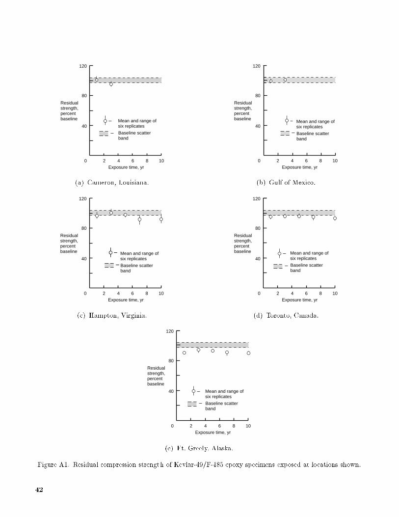
2 40
40
6 8 10Exposure time, yr
80
120
Residualstrength,percentbaseline Mean and range of
six replicates
Baseline scatterband
(a) Cameron, Louisiana.
2 40
40
6 8 10Exposure time, yr
80
120
Residualstrength,percentbaseline
Mean and range ofsix replicates
Baseline scatterband
(b) Gulf of Mexico.
2 40
40
6 8 10Exposure time, yr
80
120
Residualstrength,percentbaseline Mean and range of
six replicates
Baseline scatterband
(c) Hampton, Virginia.
2 40
40
6 8 10Exposure time, yr
80
120
Residualstrength,percentbaseline Mean and range of
six replicates
Baseline scatterband
(d) Toronto, Canada.
2 40
40
6 8 10Exposure time, yr
80
120
Residualstrength,percentbaseline
Mean and range ofsix replicates
Baseline scatterband
(e) Ft. Greely, Alaska.
Figure A1. Residual compression strength of Kevlar-49/F-185 epoxy specimens exposed at locations shown.
42

2 40
40
6 8 10Exposure time, yr
80
120
Residualstrength,percentbaseline
Mean and range ofsix replicates
Baseline scatterband
(a) Cameron, Louisiana.
2 40
40
6 8 10Exposure time, yr
80
120
Residualstrength,percentbaseline
Mean and range ofsix replicates
Baseline scatterband
(b) Gulf of Mexico.
2 40
40
6 8 10Exposure time, yr
80
120
Residualstrength,percentbaseline
Mean and range ofsix replicates
Baseline scatterband
(c) Hampton, Virginia.
2 40
40
6 8 10Exposure time, yr
80
120
Residualstrength,percentbaseline
Mean and range ofsix replicates
Baseline scatterband
(d) Toronto, Canada.
2 40
40
6 8 10Exposure time, yr
80
120
Residualstrength,percentbaseline
Mean and range ofsix replicates
Baseline scatterband
(e) Ft. Greely, Alaska.
Figure A2. Residual compression strength of Kevlar-49/CE-306 epoxy specimens exposed at locations shown.
43

2 40
40
6 8 10Exposure time, yr
80
120
Residualstrength,percentbaseline
Mean and range ofsix replicates
Baseline scatterband
(a) Cameron, Louisiana.
2 40
40
6 8 10Exposure time, yr
80
120
Residualstrength,percentbaseline
Mean and range ofsix replicates
Baseline scatterband
(b) Gulf of Mexico.
2 40
40
6 8 10Exposure time, yr
80
120
Residualstrength,percentbaseline
Mean and range ofsix replicates
Baseline scatterband
(c) Hampton, Virginia.
2 40
40
6 8 10Exposure time, yr
80
120
Residualstrength,percentbaseline
Mean and range ofsix replicates
Baseline scatterband
(d) Toronto, Canada.
2 40
40
6 8 10Exposure time, yr
80
120
Residualstrength,percentbaseline
Mean and range ofsix replicates
Baseline scatterband
(e) Ft. Greely, Alaska.
Figure A3. Residual compression strength of Kevlar-49/LRF-277 epoxy specimens exposed at locations shown.
44

2 40
40
6 8 10Exposure time, yr
80
120
Residualstrength,percentbaseline
Mean and range ofsix replicates
Baseline scatterband
(a) Cameron, Louisiana.
2 40
40
6 8 10Exposure time, yr
80
120
Residualstrength,percentbaseline
Mean and range ofsix replicates
Baseline scatterband
(b) Gulf of Mexico.
2 40
40
6 8 10Exposure time, yr
80
120
Residualstrength,percentbaseline
Mean and range ofsix replicates
Baseline scatterband
(c) Hampton, Virginia.
2 40
40
6 8 10Exposure time, yr
80
120
Residualstrength,percentbaseline
Mean and range ofsix replicates
Baseline scatterband
(d) Toronto, Canada.
2 40
40
6 8 10Exposure time, yr
80
120
Residualstrength,percentbaseline
Mean and range ofsix replicates
Baseline scatterband
(e) Ft. Greely, Alaska.
Figure A4. Residual compression strength of T-300 graphite/E-788 epoxy specimens exposed at locations
shown.
45

2 40
40
6 8 10Exposure time, yr
80
120
Residualstrength,percentbaseline
Mean and range ofsix replicates
Baseline scatterband
(a) Cameron, Louisiana.
2 40
40
6 8 10Exposure time, yr
80
120
Residualstrength,percentbaseline
Mean and range ofsix replicates
Baseline scatterband
(b) Gulf of Mexico.
2 40
40
6 8 10Exposure time, yr
80
120
Residualstrength,percentbaseline
Mean and range ofsix replicates
Baseline scatterband
(c) Hampton, Virginia.
2 40
40
6 8 10Exposure time, yr
80
120
Residualstrength,percentbaseline
Mean and range ofsix replicates
Baseline scatterband
(d) Toronto, Canada.
2 40
40
6 8 10Exposure time, yr
80
120
Residualstrength,percentbaseline
Mean and range ofsix replicates
Baseline scatterband
(e) Ft. Greely, Alaska.
Figure A5. Residual SBS strength of Kevlar-49/F-185 epoxy specimens exposed at locations shown.
46

2 40
40
6 8 10Exposure time, yr
80
120
Residualstrength,percentbaseline
Mean and range ofsix replicates
Baseline scatterband
(a) Cameron, Louisiana.
2 40
40
6 8 10Exposure time, yr
80
120
Residualstrength,percentbaseline
Mean and range ofsix replicates
Baseline scatterband
(b) Gulf of Mexico.
2 40
40
6 8 10Exposure time, yr
80
120
Residualstrength,percentbaseline
Mean and range ofsix replicates
Baseline scatterband
(c) Hampton, Virginia.
2 40
40
6 8 10Exposure time, yr
80
120
Residualstrength,percentbaseline
Mean and range ofsix replicates
Baseline scatterband
(d) Toronto, Canada.
2 40
40
6 8 10Exposure time, yr
80
120
Residualstrength,percentbaseline
Mean and range ofsix replicates
Baseline scatterband
(e) Ft. Greely, Alaska.
Figure A6. Residual SBS strength of Kevlar-49/CE-306 epoxy specimens exposed at locations shown.
47

2 40
40
6 8 10Exposure time, yr
80
120
Residualstrength,percentbaseline
Mean and range ofsix replicates
Baseline scatterband
(a) Cameron, Louisiana.
2 40
40
6 8 10Exposure time, yr
80
120
Residualstrength,percentbaseline
Mean and range ofsix replicates
Baseline scatterband
(b) Gulf of Mexico.
2 40
40
6 8 10Exposure time, yr
80
120
Residualstrength,percentbaseline
Mean and range ofsix replicates
Baseline scatterband
(c) Hampton, Virginia.
2 40
40
6 8 10Exposure time, yr
80
120
Residualstrength,percentbaseline
Mean and range ofsix replicates
Baseline scatterband
(d) Toronto, Canada.
2 40
40
6 8 10Exposure time, yr
80
120
Residualstrength,percentbaseline
Mean and range ofsix replicates
Baseline scatterband
(e) Ft. Greely, Alaska.
Figure A7. Residual SBS strength of Kevlar-49/LRF-277 epoxy specimens exposed at locations shown.
48

2 40
40
6 8 10Exposure time, yr
80
120
Residualstrength,percentbaseline
Mean and range ofsix replicates
Baseline scatterband
(a) Cameron, Louisiana.
2 40
40
6 8 10Exposure time, yr
80
120
Residualstrength,percentbaseline
Mean and range ofsix replicates
Baseline scatterband
(b) Gulf of Mexico.
2 40
40
6 8 10Exposure time, yr
80
120
Residualstrength,percentbaseline
Mean and range ofsix replicates
Baseline scatterband
(c) Hampton, Virginia.
2 40
40
6 8 10Exposure time, yr
80
120
Residualstrength,percentbaseline
Mean and range ofsix replicates
Baseline scatterband
(d) Toronto, Canada.
2 40
40
6 8 10Exposure time, yr
80
120
Residualstrength,percentbaseline
Mean and range ofsix replicates
Baseline scatterband
(e) Ft. Greely, Alaska.
Figure A8. Residual SBS strength of T-300 graphite/E-788 epoxy specimens exposed at locations shown.
49

2 40
40
6 8 10Exposure time, yr
80
120
Residualstrength,percentbaseline
Mean and range ofsix replicates
Baseline scatterband
(a) Cameron, Louisiana.
2 40
40
6 8 10Exposure time, yr
80
120
Residualstrength,percentbaseline
Mean and range ofsix replicates
Baseline scatterband
(b) Gulf of Mexico.
2 40
40
6 8 10Exposure time, yr
80
120
Residualstrength,percentbaseline
Mean and range ofsix replicates
Baseline scatterband
(c) Hampton, Virginia.
2 40
40
6 8 10Exposure time, yr
80
120
Residualstrength,percentbaseline
Mean and range ofsix replicates
Baseline scatterband
(d) Toronto, Canada.
2 40
40
6 8 10Exposure time, yr
80
120
Residualstrength,percentbaseline
Mean and range ofsix replicates
Baseline scatterband
(e) Ft. Greely, Alaska.
Figure A9. Residual tension strength of Kevlar-49/F-185 epoxy specimens exposed at locations shown.
50

2 40
40
6 8 10Exposure time, yr
80
120
Residualstrength,percentbaseline
Mean and range ofsix replicates
Baseline scatterband
(a) Cameron, Louisiana.
2 40
40
6 8 10Exposure time, yr
80
120
Residualstrength,percentbaseline
Mean and range ofsix replicates
Baseline scatterband
(b) Gulf of Mexico.
2 40
40
6 8 10Exposure time, yr
80
120
Residualstrength,percentbaseline
Mean and range ofsix replicates
Baseline scatterband
(c) Hampton, Virginia.
2 40
40
6 8 10Exposure time, yr
80
120
Residualstrength,percentbaseline
Mean and range ofsix replicates
Baseline scatterband
(d) Toronto, Canada.
2 40
40
6 8 10Exposure time, yr
80
120
Residualstrength,percentbaseline
Mean and range ofsix replicates
Baseline scatterband
(e) Ft. Greely, Alaska.
Figure A10. Residual tension strength of Kevlar-49/CE-306 epoxy specimens exposed at locations shown.
51

2 40
40
6 8 10Exposure time, yr
80
120
Residualstrength,percentbaseline
Mean and range ofsix replicates
Baseline scatterband
(a) Cameron, Louisiana.
2 40
40
6 8 10Exposure time, yr
80
120
Residualstrength,percentbaseline
Mean and range ofsix replicates
Baseline scatterband
(b) Gulf of Mexico.
2 40
40
6 8 10Exposure time, yr
80
120
Residualstrength,percentbaseline
Mean and range ofsix replicates
Baseline scatterband
(c) Hampton, Virginia.
2 40
40
6 8 10Exposure time, yr
80
120
Residualstrength,percentbaseline
Mean and range ofsix replicates
Baseline scatterband
(d) Toronto, Canada.
2 40
40
6 8 10Exposure time, yr
80
120
Residualstrength,percentbaseline
Mean and range ofsix replicates
Baseline scatterband
(e) Ft. Greely, Alaska.
Figure A11. Residual tension strength of Kevlar-49/LRF-277 epoxy specimens exposed at locations shown.
52

2 40
40
6 8 10Exposure time, yr
80
120
Residualstrength,percentbaseline
Mean and range ofsix replicates
Baseline scatterband
(a) Cameron, Louisiana.
2 40
40
6 8 10Exposure time, yr
80
120
Residualstrength,percentbaseline
Mean and range ofsix replicates
Baseline scatterband
(b) Gulf of Mexico.
2 40
40
6 8 10Exposure time, yr
80
120
Residualstrength,percentbaseline
Mean and range ofsix replicates
Baseline scatterband
(c) Hampton, Virginia.
2 40
40
6 8 10Exposure time, yr
80
120
Residualstrength,percentbaseline
Mean and range ofsix replicates
Baseline scatterband
(d) Toronto, Canada.
2 40
40
6 8 10Exposure time, yr
80
120
Residualstrength,percentbaseline
Mean and range ofsix replicates
Baseline scatterband
(e) Ft. Greely, Alaska.
Figure A12. Residual tension strength of T-300 graphite/E-788 epoxy specimens exposed at locations shown.
53

REPORT DOCUMENTATION PAGEForm Approved
OMB No. 0704-0188
Public reporting burden for this collection of information is estimated to average 1 hour per response, including the time for reviewing instructions, searching existing data sources,gathering and maintaining the data needed, and completing and reviewing the collection of information. Send comments regarding this burden estimate or any other aspect of thiscollection of information, including suggestions for reducing this burden, toWashington Headquarters Services, Directorate for Information Operations and Reports, 1215 Je�ersonDavis Highway, Suite 1204, Arlington, VA 22202-4302, and to the O�ce of Management and Budget, Paperwork Reduction Project (0704-0188), Washington, DC 20503.
1. AGENCY USE ONLY(Leave blank) 2. REPORT DATE 3. REPORT TYPE AND DATES COVERED
September 1994 Technical Paper
4. TITLE AND SUBTITLE
Ten-Year Ground Exposure of Composite Materials Usedon the Bell Model 206L Helicopter Flight Service Program
6. AUTHOR(S)
Donald J. Baker
7. PERFORMING ORGANIZATION NAME(S) AND ADDRESS(ES)
Vehicle Structures DirectorateU.S. Army Research LaboratoryNASA Langley Research CenterHampton, VA 23681-0001
9. SPONSORING/MONITORING AGENCY NAME(S) AND ADDRESS(ES)
National Aeronautics and Space AdministrationWashington, DC 20546-0001
andU.S. Army Research LaboratoryAdelphi, MD 20783-1145
5. FUNDING NUMBERS
WU 532-06-37-03
PR 1L162211A47AB
8. PERFORMING ORGANIZATION
REPORT NUMBER
L-17341
10. SPONSORING/MONITORING
AGENCY REPORT NUMBER
NASA TP-3468
ARL-TR-480
11. SUPPLEMENTARY NOTES
12a. DISTRIBUTION/AVAILABILITY STATEMENT 12b. DISTRIBUTION CODE
Unclassi�ed{Unlimited
Subject Category 24
13. ABSTRACT (Maximum 200 words)
Residual strength results are presented for four composite material systems that have been exposed for up to10 years to the environment at �ve di�erent locations on the North American continent. The exposure locationsare near where the Bell Model 206L helicopters, which participated in a ight service program sponsored byNASA Langley Research Center and the U.S. Army, were ying in daily commercial service. The compositematerial systems are (1) Kevlar-49 fabric/F-185 epoxy; (2) Kevlar-49 fabric/LRF-277 epoxy; (3) Kevlar-49fabric/CE-306 epoxy; and (4) T-300 graphite/E-788 epoxy. Six replicates of each material were removed andtested after 1, 3, 5, 7, and 10 years of exposure. The average baseline strength was determined from testingsix as-fabricated specimens. More than 1700 specimens have been tested. All specimens that were testedto determine their strength were painted with a polyurethane paint. Each set of specimens also includedan unpainted panel for observing the weathering e�ects on the composite materials. A statistically basedprocedure has been used to determine the strength value above which at least 90 percent of the population isexpected to fall with a 95-percent con�dence level. The computed compression strengths are 80 to 89 percent ofthe baseline (no-exposure) strengths. The resulting compression strengths are approximately 8 percent belowthe population mean strengths. The computed short-beam-shear strengths are 83 to 92 percent of the baseline(no-exposure) strengths. The computed tension strength of all materials is 93 to 97 percent of the baseline(no-exposure) strengths.
14. SUBJECT TERMS 15. NUMBER OF PAGES
Composite materials; Environmental exposure; Material properties 54
16. PRICE CODE
A0417. SECURITY CLASSIFICATION 18. SECURITY CLASSIFICATION 19. SECURITY CLASSIFICATION 20. LIMITATION
OF REPORT OF THIS PAGE OF ABSTRACT OF ABSTRACT
Unclassi�ed Unclassi�ed Unclassi�ed
NSN 7540-01-280-5500 Standard Form 298(Rev. 2-89)Prescribed by ANSI Std. Z39-18298-102