Ten modules to teach controls from the basic to advanced

STUDENT WorkbookFlexible Joint Experiment for MaTLab®/Simulink® Users

Standardized for ABET* Evaluation Criteria

Developed by:Jacob Apkarian, Ph.D., QuanserPaul Karam, B.A.SC., QuanserMichel Lévis, M.A.SC., Quanser

With the SRV02 Base Unit, you can select from 10 add-on modules to create experiments of varying complexity across a wide range of topics, disciplines and courses. All of the experiments/workstations are compatible with MATLAB®/Simulink®.

To request a demonstration or a quote, please email [email protected].

©2012 Quanser Inc. All rights reserved. MATLAB® and Simulink® are registered trademarks of The MathWorks Inc.

SrV02 base Unit Flexible Link Inverted Pendulum ball and beam

Multi-DoF Torsion2 DoF Inverted Pendulum2 DoF robot

Flexible Joint Gyro/Stable Platform Double Inverted Pendulum 2 DoF ball balancer

Student W

orkbook: Flexible Joint Exp

eriment for M

aTLa

b®/

Sim

ulink® U

sers

Ten modules to teach controls from the basic to advanced level

SRV02 educational solutions are powered by:

Course material complies with:

CaPTIVaTE. MoTIVaTE. GraDUaTE. Solutions for teaching and research. Made in Canada.

[email protected] +1-905-940-3575 QUaNSEr.CoM * ABET Inc., is the recognized accreditor for college and university programs in applied science, computing, engineering, and technology. Among the most respected accreditation organizations in the U.S., ABET has provided leadership and quality assurance in higher education for over 75 years.

c⃝ 2011 Quanser Inc., All rights reserved.

Quanser Inc.119 Spy CourtMarkham, OntarioL3R [email protected]: 1-905-940-3575Fax: 1-905-940-3576

Printed in Markham, Ontario.

For more information on the solutions Quanser Inc. offers, please visit the web site at:http://www.quanser.com

This document and the software described in it are provided subject to a license agreement. Neither the software nor this document may beused or copied except as specified under the terms of that license agreement. All rights are reserved and no part may be reproduced, stored ina retrieval system or transmitted in any form or by any means, electronic, mechanical, photocopying, recording, or otherwise, without the priorwritten permission of Quanser Inc.

ACKNOWLEDGEMENTSQuanser, Inc. would like to thank Dr. Hakan Gurocak, Washington State University Vancouver, USA, for his help to include embedded out-comes assessment.

ROTFLEX Workbook - Student Version 2

http://www.quanser.com

CONTENTS1 Introduction 4

2 Modeling 52.1 Background 52.2 Pre-Lab Questions 112.3 Lab Experiments 122.4 Results 17

3 Control Design 183.1 Specifications 183.2 Background 183.3 Pre-Lab Questions 233.4 Lab Experiments 243.5 Results 28

4 System Requirements 294.1 Overview of Files 304.2 Setup for Finding Stiffness 304.3 Setup for Model Validation 314.4 Setup for Flexible Joint Control Simulation 314.5 Setup for Flexible Joint Control Implementation 32

5 Lab Report 335.1 Template for Content (Modeling) 335.2 Template for Content (Control) 345.3 Tips for Report Format 36

ROTFLEX Workbook - Student Version v 1.0

1 INTRODUCTIONThe objective of this experiment is to control the position of the servo while minimizing the motions the flexible rotarylink.

Topics Covered

• Modeling the Rotary Flexible Joint using Lagrange.

• Find the linear state-space model of the system.

• Do some basic model validation.

• Design a state-feedback controller using Pole-Placement (PP).

• Simulate the closed-loop flexible joint system.

• Implement the designed controller on the device.

• Compare the simulated and measured closed-loop results.

• Assess the behaviour of implementing a partial-state feedback controller.

Prerequisites

In order to successfully carry out this laboratory, the user should be familiar with the following:

• Basics of Simulinkr.

• Transfer function fundamentals.

• State-space modeling, e.g., obtaining state equations from a set of differential equations.

• SRV02 QUARC Integration Laboratory ([3]) in order to be familiar using QUARCrwith the SRV02.


2 MODELING

2.1 Background

2.1.1 Model

The Rotary Flexible Joint model is shown in Figure 2.1. The base of the module is mounted on the load gear of theSRV02 system. The servo angle, θ, increases positively when it rotates counter-clockwise (CCW). The servo (andthus the link) turn in the CCW direction when the control voltage is positive, i.e., Vm > 0.

The total length of the link can be varied by changing the mounting position of the shorter top arm. The main bottomarm, which is connected to the pivot, has a length of L1 and a mass of m1. The length and mass of the top link isL2 andm2. The distance between the pivot and the middle of the top arm, which can be changed, is denoted by thevariable d12. The moment of inertia of the entire link is specified by Jl and it changes depending on the position ofthe top arm. See the Rotary Flexible Joint User Manual (in [7]) for the values of these parameters. The deflectionangle of the link is denoted as α and increases positively when rotated CCW.

Figure 2.1: Rotary Flexible Joint Angles

The flexible joint system can be represented by the diagram shown in Figure 2.2. Our control variable is the inputservo motor voltage, Vm. This generates a torque, τ , at the load gear of the servo that rotates the base of the link.The viscous friction coefficient of the servo is denoted by Beq. This is the friction that opposes the torque beingapplied at the servo load gear. The friction acting on the link is represented by the viscous damping coefficient Bl.Finally, the flexible joint is modeled as a linear spring with the stiffness Ks.

Figure 2.2: Rotary Flexible Joint Model


2.1.2 Finding the Equations of Motion

Instead of using classical mechanics, the Lagrange method is used to find the equations of motion of the system.This systematic method is often used for more complicated systems such as robot manipulators with multiple joints.

More specifically, the equations that describe the motions of the servo and the link with respect to the servo motorvoltage, i.e. the dynamics, will be obtained using the Euler-Lagrange equation:

∂2L

∂t∂qi− ∂L

∂qi= Qi (2.1)

The variables qi are called generalized coordinates. For this system let

q(t)⊤ = [θ(t) α(t)] (2.2)

where, as shown in Figure 2.2, θ(t) is the servo angle and α(t) is the flexible joint angle. The corresponding velocitiesare

q(t)⊤ =

[∂θ(t)

∂t

∂α(t)

∂t

]

Note: The dot convention for the time derivative will be used throughout this document, i.e., θ = dθdt and α = dα

dt .The time variable t will also be dropped from θ and α, i.e., θ := θ(t) and α := α(t).

With the generalized coordinates defined, the Euler-Lagrange equations for the rotary flexible joint system are

∂2L

∂t∂θ− ∂L

∂θ= Q1 (2.3)

and∂2L

∂t∂α− ∂L

∂α= Q2 (2.4)

The Lagrangian of a system is definedL = T − V (2.5)

where T is the total kinetic energy of the system and V is the total potential energy of the system. Thus the Lagrangianis the difference between a system's kinetic and potential energies.

The generalized forces Qi are used to describe the non-conservative forces (e.g., friction) applied to a system withrespect to the generalized coordinates. In this case, the generalized force acting on the rotary arm is

Q1 = τ −Beq θ (2.6)

and acting on the link isQ2 = −Blα. (2.7)

The torque applied at the base of the rotary arm (i.e., at the load gear) is generated by the servo motor as describedby the equation

τ =ηgKgηmkt(Vm −Kgkmθ)

Rm. (2.8)

See [5] for a description of the corresponding SRV02 parameters (e.g. such as the back-emf constant, km). Theservo damping (i.e. friction), Beq, opposes the applied torque. The flexible joint is not actuated, the only force actingon the link is the damping, Bl.

Again, the Euler-Lagrange equations is a systematic method of finding the equations of motion (EOMs) of a system.Once the kinetic and potential energy are obtained and the Lagrangian is found, then the task is to compute variousderivatives to get the EOMs.


2.1.3 Potential and Kinetic Energy

Kinetic EnergyTranslational kinetic equation is defined as

T =1

2mv2, (2.9)

where m is the mass of the object and v is the linear velocity.

Rotational kinetic energy is described asT =

1

2Jω2 (2.10)

where J is the moment of inertia of the object and ω is its angular rate.

Potential EnergyPotential energy comes in different forms. Typically in mechanical system we deal with gravitational and elasticpotential energy. The relative gravitational potential energy of an object is

Vg = mg∆h, (2.11)

where m is the object mass and ∆h is the change in altitude of the object (from a reference point). The potentialenergy of an object that rises from the table surface (i.e., the reference) up to 0.25 meter is ∆h = 0.25 − 0 = 0.25and the energy stored is Vg = 0.25mg.

The equation for elastic potential energy, i.e., the energy stored in a spring, is

Ve =1

2K∆x2 (2.12)

where K is the spring stiffness and ∆x is the linear or angular change in position. If an object that is connected toa spring moves from in its initial reference position to 0.1 m, then the change in displacement is ∆x = 0.1− 0 = 0.1and the energy stored equals Ve = 0.005K.

2.1.4 Linear State-Space Model

The linear state-space equations arex = Ax+Bu (2.13)

andy = Cx+Du (2.14)

where x is the state, u is the control input, A, B, C, and D are state-space matrices. For the Rotary Flexible Jointsystem, the state and output are defined

x⊤ = [θ α θ α] (2.15)

andy⊤ = [x1 x2]. (2.16)

In the output equation, only the position of the servo and link angles are being measured. Based on this, the C andD matrices in the output equation are

C =

[1 0 0 00 1 0 0

](2.17)

andD =

[00

]. (2.18)

The velocities of the servo and link angles can be computed in the digital controller, e.g., by taking the derivativeand filtering the result though a high-pass filter.


2.1.5 Finding Second Order System Parameters

Consider a second-order system described by

Jx+Bx+Kx = 0. (2.19)

Assuming the initial conditions x(0−) = x0 and x(0−) = 0, the Laplace transform of Equation 2.19 is

X(s) =x0

J

s2 + BJ s+

KJ

(2.20)

The prototype second-order equation is defined

s2 + 2ζωns+ ω2n,

where ζ is the damping ratio and ωn is the natural frequency. Equating the characteristic equation in 2.20 to thisgives

ω2n =

K

J

and2ζωn =

B

J

Based on the measured damping ratio and natural frequency, the friction (or stiffness) of the system is

K = Jω2n (2.21)

and the viscous damping isB = 2ζωnJ. (2.22)

The natural frequency and damping ratio of a system can be found experimentally, e.g., from a free-oscillationresponse or frequency response.

2.1.6 Power Spectrum

Fourier is a way to represent a signal in terms of sinusoidals. The Fourier transform, or spectrum, of a signal g(t) isdenoted as G(ω) and it shows the relative amplitudes and frequencies of the sinusoidals that are used to representthat signal [9].

The Fourier transform contains both the magnitude and phase information. The power spectrum of a signal is basedon the magnitude of the signal. Figure 2.3, for example, show the power spectrum of the compound sine wave signal

g(t) = 3 sin 2πt+ 2 sin 4πt+ 0.5 sin 10πt.

The spectrum shows the peaks occurring at the sine wave frequencies 1, 2, and 5 Hz. Similarly, this can be used tofind the resonant frequencies of an actual system.

The power of a signal is the time-average of the its squared value [9] and, for a continuous signal g(t), is defined

Pg = limT→∞

1

T

∫ T/2

−T/2

g(t)2dt.

We want to define the power of the signal from its transform. First consider the truncated signal of g(t) defined as

gT (t) =

{g(t) |t| ≤ T

0 |t| > T


Figure 2.3: Power spectrum of compound sine wave

From Parseval's theorem, the energy of this signal equals [9]

EgT =

∫ ∞

−∞gT (t)

2dt =1

2π

∫ ∞

−∞|GT (ω)|2dω

The power of a signal can then be expressed as

Pg = limT→∞

EgT

T

=1

2πlim

T→∞

∫ ∞

−∞

|GT (ω)|2

Tdω.

The power spectral density (PSD) function is

Sg(ω) = limT→∞

|GT (ω)|2

T(2.23)

Defining the signal power in terms of the PSD and considering only positive frequencies we get

Pg =1

2π

∫ ∞

−∞Sg(ω)dω

=1

π

∫ ∞

0

Sg(ω)dω

Expressing this in term of Hertz we get the expression

Pg = 2

∫ ∞

0

Sg(ω)df (2.24)

In practice, signals are sampled and the algorithm is performed in discrete mode. The Fast-Fourier Transform(FFT) is a computational algorithm used to find the Fourier transform of a signal, i.e., taking the FFT of a signal g(t)generates G(ω). To find the power spectrum, code similar to the following would be used


y = fft(g);Sg = |y|/N;Pg = 2*Sg(1:N/2);

whereN is the number of samples, or length, of the signal g(t). If g(t) was sampled at a frequency interval of Ts andhad a duration of T , it would have N = T/Ts samples. Notice that because this is implemented in discrete mode,we use the amount of samples, N , instead of the signal time duration, T , as used in the PSD expression in Equation2.23.

The power spectrum can be used to find resonant frequencies of a system. One common technique is feeding asine sweep (or chirp) signal to the system and measuring the corresponding output response. By taking its FFTand finding the spectrum, the user will see various peaks. These peaks represent the sine wave frequencies thatdescribe the system.


2.2 Pre-Lab Questions

1. Energy is stored in the flexible joint springs as it rotates by an angle of α (see Figure 2.1). Find the potentialenergy of the flexible joint using the parameters described in Section 2.1.

2. Find the total kinetic energy of the system contributed by the rotary servo, θ, and the rotation of the link, α.Use the parameters shown in Figure 2.2.

3. Compute the Lagrangian of the system.

4. Find the first Euler-Lagrange equation given in 2.3. Keep the equations in terms of applied torque, τ (i.e., notin terms of DC motor voltage). Also make sure your equations follow the general form: Jx+Bx+Kx = u.

5. Find the second Euler-Lagrange Equation 2.4.

6. Find the equations of motion: θ = f1(θ, θ, α, α, τ) and α = f2(θ, θ, α, α, τ). Assume the viscous damping of thelink is negligible, i.e., Bl = 0.

7. Given state x defined in Equation 2.15, find the linear state-space matrices A and B.

8. Express the moment of inertia of the rotary arm in terms of the length and masses given in Figure 2.1. Asalready mentioned, the total arm length varies depending on where the short arm is mounted on top of thelong arm. The inertia can be computed in the lab once you know how your ROTFLEX is configured.Hint: The total inertia depends on where the top arm is anchored. Use the parallel-axis theorem to determinethe inertia of the top link with respect to the pivot.


2.3 Lab Experiments

In the first part of this laboratory, the stiffness of the flexible joint is determined by measuring its natural frequency.In the second part, the state-space model is finalized and validated against actual measurements.

2.3.1 Finding Stiffness

To find the stiffness we need to find the natural frequency of the flexible joint. This is the frequency where the linkattached to the flexible joint begins to oscillate the most. To find this frequency, we use a Sine Sweep signal. TheSine Sweep is a sine wave that goes through a range of frequencies, i.e., from low to high. We can then generatea power spectrum from the measured signal and identify the frequency with the largest amplitude - the naturalfrequency.

Physical Parameters for the Lab

In order to do some of the laboratory exercises, you will need these values:

Beq = 0.004 N · m / (rad/s)Jeq = 2.08× 10−3 kg · m2

m1 = 0.064 kgL1 = 0.298 mm2 = 0.030 kgL2 = 0.156 mBl = 0

Note: The equivalent viscous damping, Beq, and moment of inertia, Jeq, parameters are for the SRV02 when thereis no load (i.e., the parameter found in the SRV02 Modeling Laboratory was for servo with the disc load).

Experimental Setup

The q rotflex id Simulink diagram shown in Figure 2.4 is used to find the natural frequency of the flexible joint.The QUARC blocks are used to interface with the DC motor and encoders of the system. The Sine Sweep blockgenerates a sine wave that goes from a low frequency to a high frequency for a predetermined duration. For moreinformation about the QUARCrsoftware, see Reference [3]. This model outputs the deflection angle of the link.

Figure 2.4: q rotflex id Simulink diagram used to find flexible joint stiffness

IMPORTANT: Before you can conduct this experiment, you need to make sure that the lab files are configured


according to your system setup. If they have not been configured already, then you need to go to Section 4.2 toconfigure the lab files first.

1. In the q rotflex id Simulink diagram, go to QUARC | Build to build the QUARC controller.

2. Go to QUARC | Start to run the controller. The SRV02 tracks a sine sweep that goes from 1 Hz to 5 Hz. Thealpha (deg) Scope should be reading a response similarly as shown in Figure 2.5. Note that the controller isset to run for 15 seconds.

Figure 2.5: Typical Flexible Joint Sine Sweep Response

3. After the controller stops (i.e., after 15 sec), the data is automatically saved in the Matlab workspace to thevariable data alpha. The time is stored in data alpha(:,1) vector and the link angle is stored the data alpha(:,2)vector. Plot the response in a Matlab figure.

4. Using the sweep response data and Matlab commands, generate a plot of the power spectrum. The back-ground theory and pseudo code to find the power spectrum was given in Section 2.1.6. You can also use anyavailable Matlab examples to help you out. Show the commands you used and the plot generated.Hint: When using the discrete Matlab FFT command fft(x,n), the size of n should be base of 2. Use thenextpow2 function to find this size. For example, if your signal size is 250 samples long, this will return 8 whichgives n = 28 = 256.

5. Find the natural frequency of the link. Because the damping in relatively low, assume the damped naturalfrequency (which is being measured) is equivalent to the undamped natural frequency.

6. Find the total moment of inertia of the link, Jl, using the equation you developed in the Exercise 8 in Section2.2. The corresponding value of d12 is given in the Rotary Flexible Joint User Manual [7]. Once the inertia iscomputed, find the stiffness of the flexible joint, Ks.

2.3.2 Model Validation

By running a simulation and the actual device in parallel, we can verify whether the dynamic model (which drivesthe simulation) accurately represents our system.

Experimental Setup

The q rotflex val Simulink diagram shown in Figure 2.6 applies either a step or pulse input to both the QuanserFlexible Joint hardware and to the Flexible Joint model and reads the servo and link angles. The SRV02 FlexibleJoint subsystem contains the QUARC blocks that interface to the actual hardware. The Simulink State-Space blockreads the A, B, C, and D state-space matrices that are loaded in the Matlab workspace. This model outputs thedeflection angle of the link.


Figure 2.6: q rotflex val Simulink diagram used validate the model

IMPORTANT: Before you can conduct this experiment, you need to make sure that the lab files are configuredaccording to your system setup. If they have not been configured already, then go to Section 4.3 to configure thelab files first.

1. Run the setup rotflex.m.

2. When prompted, enter the stiffness you found in Section 2.3.1. This is saved to the Matlab variable Ks.

Enter link stiffness (Ks):

3. Depending on your stiffness, the Matlab prompt should generate a gain similarly as shown below (this gain isgenerated for a Ks of 1):

K =

0 0 0 0

cls_poles =

0 0 0 0

This means the script ran correctly.

4. In Matlab, open the M-File called ROTFLEXE ABCD eqns student.m. The script has the following state-spacematrices entered:

A = [0 0 1 0;0 0 0 1;0 500 -5 0;0 -750 5 0];

B = [0 0 500 -500]';

C = zeros(2,4);

D = zeros(2,1);


5. Enter the state-space matrices you found in Section 2.2 for A, B, C, and D. In Matlab, the stiffness and linkmoment of inertia are defined as Ks and Jl and the SRV02 inertia and damping are denoted Jeq and Beq.

6. Run the ROTFLEX ABCD eqns student.m script to load the state-space matrices in the Matlab workspace.Show the numerical matrices that are displayed in the Matlab prompt.

7. The input of the state-space model you found in Section 2.2 is the torque acting at the servo load gear (i.e., atthe pivot of the flexible joint). However, we do not control torque directly - we control the servo input voltage.Recall the voltage-torque relationship given in Equation 2.8 in Section 2.1.2. In the System Model section ofthe setup rotflex.m script, the actuator dynamics are added to your state-space matrices with the code:

Ao = A;Bo = B;B = eta_g*Kg*eta_m*kt/Rm*Bo;A(3,3) = Ao(3,3) - Bo(3)*eta_g*Kg^2*eta_m*kt*km/Rm;A(4,3) = Ao(4,3) - Bo(4)*eta_g*Kg^2*eta_m*kt*km/Rm;

8. Run the setup rotflex.m script again so your Flexible Joint model is based on DC motor voltage.

9. In the q rotflex val Simulink diagram, go to QUARC | Build to build the QUARC controller.

10. Make sure the area around the Flexible Joint experiment is clear. Set the Manual Switch to the downwardposition to feed a Step input.

11. Go to QUARC | Start to run the q rotflex val controller. Typical scope responses are shown in Figure 2.7. Thetheta (deg) scope displays the simulated servo angle in yellow and the measured angle in purple. Similarly,the alpha (deg) scope shows the simulated link angle in yellow and the measured angle in purple.

(a) Servo Angle (b) Flexible Link Angle

Figure 2.7: Typical Flexible Joint model validation response in scopes

12. If your simulation and measured response match, go to the next step. If they do not, then there is an issuewith your model. Here are some issues to investigate:

• Ensure the state-space model was enterred properly in the script.• The stiffness, Ks, found in Section 2.3.1 is not correct. Review your calculations or redo the experiment.• Review your model derivation in Section 2.2, e.g., might be a mistake in solving the EOMs.

13. The theta (deg) and alpha (deg) scopes save their data to the variables data theta and data alpha. Fordata theta, the time is in data theta(:,1), the simulated servo angle is in data theta(:,2), and the measuredSRV02 angle is in data theta(:,3). Similarly for the flexible joint response saved in data alpha. Plot the re-sponse in a Matlab figure.

14. How well does your model represent the actual system? We want a model that is fairly representative but,having said that, keep in mind that no model is perfect. This is just a quick test to see how well your modelrepresents the actual device. As shown in figures 2.7a and 2.7b, the simulation does not match the measuredresponse perfectly.


15. Give at least one reason why the model does not represent the system accurately.

16. In Matlab, find the open-loop poles (i.e., eigenvalues) of the system using the state-space matrix A that isloaded.Note: These will be required for a pre-lab question in Section 3.3.


2.4 Results

Fill out Table 1 with your answers from your modeling lab results - both simulation and implementation.

Description Symbol Value UnitFinding StiffnessNatural frequency ωn rad/sStiffness Ks N m/radModel Validation

State-Space Matrix A

State-Space Matrix B

State-Space Matrix C

State-Space Matrix D

Open-loop poles OL

Table 1: Results


3 CONTROL DESIGN

3.1 Specifications

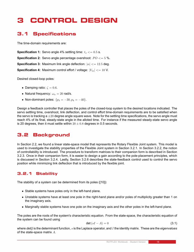
The time-domain requirements are:

Specification 1: Servo angle 4% settling time: ts <= 0.5 s.

Specification 2: Servo angle percentage overshoot: PO <= 5 %.

Specification 3: Maximum link angle deflection: |α| <= 12.5 deg.

Specification 4: Maximum control effort / voltage: |Vm| <= 10 V.

Desired closed-loop poles:

• Damping ratio: ζ = 0.6.

• Natural frequency: ωn = 20 rad/s.

• Non-dominant poles: {p3 = −30, p4 = −40}.

Design a feedback controller that places the poles of the closed-loop system to the desired locations indicated. Theservo settling time, overshoot, link deflection, and control effort time-domain requirements are to be satisfied whenthe servo is tracking a±20 degree angle square wave. Note for the settling time specifications, the servo angle mustreach 4% of its final, steady-state angle in the alloted time. For instance if the measured steady-state servo angleis 20 degrees, then it must settle within 20± 0.8 degrees in 0.5 seconds.

3.2 Background

In Section 2.2, we found a linear state-space model that represents the Rotary Flexible Joint system. This model isused to investigate the stability properties of the Flexible Joint system in Section 3.2.1. In Section 3.2.2, the notionof controllability is introduced. The procedure to transform matrices to their companion form is described in Section3.2.3. Once in their companion form, it is easier to design a gain according to the pole-placement principles, whichis discussed in Section 3.2.4. Lastly, Section 3.2.6 describes the state-feedback control used to control the servoposition while minimizing link deflection that is introduced by the flexible joint.

3.2.1 Stability

The stability of a system can be determined from its poles ([10]):

• Stable systems have poles only in the left-hand plane.

• Unstable systems have at least one pole in the right-hand plane and/or poles of multiplicity greater than 1 onthe imaginary axis.

• Marginally stable systems have one pole on the imaginary axis and the other poles in the left-hand plane.

The poles are the roots of the system's characteristic equation. From the state-space, the characteristic equation ofthe system can be found using

det (sI −A) = 0 (3.1)where det() is the determinant function, s is the Laplace operator, and I the identity matrix. These are the eigenvaluesof the state-space matrix A.


3.2.2 Controllability

If the control input, u, of a system can take each state variable, xi where i = 1 . . . n, from an initial state to a finalstate then the system is controllable, otherwise it is uncontrollable ([10]).

Rank Test The system is controllable if the rank of its controllability matrix

T =[B AB A2B . . . AnB

](3.2)

equals the number of states in the system,rank(T ) = n. (3.3)

3.2.3 Companion Matrix

If (A,B) are controllable and B is n× 1, then A is similar to a companion matrix ([1]). Let the characteristic equationof A be

sn + ansn−1 + . . .+ a1.

Then the companion matrices of A and B are

A =

0 1 · · · 0 00 0 · · · 0 0...

.... . .

......

0 0 · · · 0 1−a1 −a2 · · · −an−1 −an

(3.4)

and

B =

0...01

(3.5)

DefineW = T T−1

where T is the controllability matrix defined in Equation 3.2 and

T = [B BA . . . BAn].

ThenW−1AW = A

andW−1B = B.

3.2.4 Pole Placement

If (A,B) are controllable, then pole placement can be used to design the controller. Given the control law u = −Kx,the state-space in Equation 2.13 becomes

x = Ax+B(−Kx)

= (A−BK)x


To illustate how to design gain K, consider the following system

A =

0 1 00 0 13 −1 −5

(3.6)

and

B =

001

(3.7)

Note that A and B are already in the companion form. We want the closed-loop poles to be at [−1 − 2 − 3]. Thedesired characteristic equation is therefore

(s+ 1)(s+ 2)(s+ 3) = s3 + 6s2 + 11s+ 6 (3.8)

For the gain K = [k1 k2 k3], apply control u = −Kx and get

A−KB =

0 1 00 0 1

3− k1 −1− k2 −5− k3

.

The characteristic equation of A−KB is

s3 + (k3 + 5)s2 + (k2 + 1)s+ (k1 − 3) (3.9)

Equating the coefficients between Equation 3.9 and the desired polynomial in Equation 3.8

k1 − 3 = 6

k2 + 1 = 11

k3 + 5 = 6

Solving for the gains, we find that a gain of K = [9 10 1] is required to move the poles to their desired location.

We can generalize the procedure to design a gain K for a controllable (A,B) system as follows:

Step 1 Find the companion matrices A and B. Compute W = T T−1.

Step 2 Compute K to assign the poles of A − BK to the desired locations. Applying the control law u = −Kx tothe general system given in Equation 3.4,

A =

0 1 · · · 0 00 0 · · · 0 0...

.... . .

......

0 0 · · · 0 1−a1 − k1 −a2 − k2 · · · −an−1 − kn−1 −an − kn

(3.10)

Step 3 Find K = KW−1 to get the feedback gain for the original system (A,B).

Remark: It is important to do the K → K conversion. Remember that (A,B) represents the actual system while thecompanion matrices A and B do not.


3.2.5 Desired Poles

The rotary inverted pendulum system has four poles. As depicted in Figure 3.1, poles p1 and p2 are the complexconjugate dominant poles and are chosen to satisfy the natural frequency, ωn, and damping ratio, ζ, specificationsgiven in Section 3.1. Let the conjugate poles be

p1 = −σ + jωd (3.11)

andp2 = −σ − jωd (3.12)

where σ = ζωn and ωd = ωn

√1− ζ2 is the damped natural frequency. The remaining closed-loop poles, p3 and p4,

are placed along the real-axis to the left of the dominant poles, as shown in Figure 3.1.

Figure 3.1: Desired closed-loop pole locations

3.2.6 Feedback Control

The feedback control loop that in Figure 3.2 is designed to stabilize the servo to a desired position, θd, while mini-mizing the deflection of the flexible link.

The reference state is definedxd = [θd 0 0 0] (3.13)

and the controller isu = K(xd − x). (3.14)

Note that if xd = 0 then u = −Kx, which is the control used in the control algorithm.


Figure 3.2: State-feedback control loop


3.3 Pre-Lab Questions

1. Based on your analysis in Section 2.3, is the system stable, marginally stable, or unstable? Did you expectthe stability of the Rotary Flexibe Joint system to be as what was determined? If desired, use your experiencewith the actual device in the Modeling Laboratory in Section 2.3.

2. Using the open-loop poles, find the characteristic equation of the system.

3. Give the corresponding companion matrices A and B. Do not compute the transformation matrix W (this willbe computed using software in the lab).

4. Find the location of the two dominant poles, p1 and p2, based on the specifications given in Section 3.1. Placethe other poles at p3 = −30 and p4 = −40. Finally, give the desired characteristic equation.

5. When applying the control u = −Kx to the companion form, it changes (A, B) to (A− BK, B). Find the gainK that assigns the poles to their new desired location.


3.4 Lab Experiments

3.4.1 Control Design

1. Run the setup rotflex.m script to load the model you found in the Modeling Experiment in Section 2.3.

2. Using Matlab commands, determine if the system is controllable. Explain why.

3. Open the d pole placement student.m script. As shown below, the companion matrices A and B for the modelare automatically found (denoted as Ac and Bc in Matlab).

% Characteristic equation: s^4 + a_4*s^3 + a_3*s^2 + a_2*s + a_1a = poly(A);%% Companion matrices (Ac, Bc)Ac = [ 0 1 0 0;

0 0 1 0;0 0 0 1;-a(5) -a(4) -a(3) -a(2)];

%Bc = [0; 0; 0; 1];% ControllabilityT = 0;% Controllability of companion matricesTc = 0;% Transformation matricesW = 0;

In order to find the gain K, we need to find the transformation matrix W = T T−1 (note: T is denoted as Tc inMatlab). Modify the d pole placement student.m script to calculate the controllability matrix T , the companioncontrollabilty matrix Tc, the inverse of Tc, and W . Show your completed script and the resulting T , Tc, Tc−1,and W matrices.

4. Enter the companion gain, K, you found in the pre-lab as Kc in d pole placement student.m and modify it tofind gain K using the transformation detailed in Section 3.2. Run the script again to calculate the feedbackgain K and record its value in Table 2.

5. Evaluate the closed-loop poles of the system, i.e., the eigenvalues of A−BK. Record the closed-loop polesof the system when using the gainK calculated above. Have the poles been placed to their desired locations?If not, then go back and re-investigate your control design until you find a gain that positions the poles to therequired location.

6. In the previous exercises, gain K was found manually through matrix operations. All that work can instead bedone using a pre-defined Compensator DesignMatlab command. Find gainK using a Matlab pole-placementcommand and verify that the gain is the same as generated before.

3.4.2 Control Simulation

Using the linear state-space model of the system and the designed control gain, the closed-loop response can besimulated. This way, we can test the controller and see if it satisfies the given specifications before running it on thehardware platform.

Experiment Setup

The s rotflex Simulink diagram shown in Figure 3.3 is used to simulate the closed-loop response of the Flexible Jointusing the control developed in Section 3.3.


The Smooth Signal Generator block generates a 0.33 Hz square wave (with amplitude of 1) that is passed through aRate Limiter block to smooth the signal. The Amplitude (deg) gain block is used to change the desired servo positioncommand. The state-feedback gainK is set in the Controller gain block and is read from the Matlab workspace. TheSimulink State-Space block reads the A, B, C, andD state-space matrices that are loaded in the Matlab workspace.

Figure 3.3: s rotflex Simulink diagram used to simulate the state-feedback control

IMPORTANT: Before you can conduct this experiment, you need to make sure that the lab files are configuredaccording to your system setup. If they have not been configured already, go to Section Section 4.4 to configure thelab files first. Make sure the model you found in Section 2.3.2 is entered in ROTFLEX ABCD eqns student.mand the d pole placement student.m calculates the control gain.

1. Run setup rotpen.m. Ensure the gain K you found in Section 3.4.1 is loaded.

2. In s rotflex, make sure the Manual Switch is set to the Full-State Feedback (upward) position.

3. Run s rotflex to simulate the closed-loop response with this gain. The response in the scopes shown in Figure3.4 were generated using an arbitary gain. Plot the simulated response of the servo, link, and motor inputvoltage obtained using your obtained gain K in a Matlab figure and attach it to your report.Note: When the simulation stops, the last 10 seconds of data is automatically saved in the Matlab workspaceto the variables data theta, data alpha, and data Vm. The time is stored in the data theta(:,1) vector, the de-sired and measured rotary arm angles are saved in the data theta(;,2) and data theta(;,3) arrays, the pendulumangle is stored the data alpha(:,2) vector, and the control input is in the data vm(:,2) structure.

4. Measure the settling time and percentage overshoot of the simulated servo response, the maximum link de-flection, and the voltage used. Does the response satisfy the specifications given in Section 3.1?

3.4.3 Control Implementation

In this experiment, the servo position is controlled while minimizing the link deflection using the control found inSection 3.4.1. Measurements will then be taken to ensure that the specifications are satisfied.

Experiment Setup

The q rotflex Simulink diagram shown in Figure 3.5 is used to run the state-feedback control on the Quanser FlexibleJoint system. The SRV02 Flexible Joint subsystem contains QUARC blocks that interface with the DC motor andsensors of the system. The feedback developed in Section 3.4.1 is implemented using a Simulink Gain block.

IMPORTANT: Before you can conduct this experiment, you need to make sure that the lab files are configuredaccording to your system setup. If they have not been configured already, then go to Section 4.5 to configure thelab files first.



(a) Servo Angle (b) Flexible Link Angle

(c) Voltage

Figure 3.4: Default Simulated Closed-Loop Response

2. Ensure the controller you found in Section 3.4.1 is loaded, i.e., gain K.

3. Open the q rotflex Simulink diagram. Make sure theManual Switch is set to the Full-State Feedback (upward)position.

4. Go to QUARC | Build to build the controller.

5. Go to QUARC | Start to run the controller. The flexible link should be tracking the default ± 20 degree signal.

6. Stop the controller once you have obtained a representative response.

7. Plot the responses from the theta (deg), alpha (deg), and Vm (V) scopes in a Matlab figure. Similarly asdescribed in Section 3.4.2, the response data is saved in variables data theta, data alpha, and data vm.

8. Measure the settling time and percentage overshoot of the measured servo response and the maximum linkdeflection. Does the response satisfy the specifications given in Section 3.1?

3.4.4 Implementing Partial-State Feedback Control

In this section, the partial-state feedback response of the system is assessed and compared with the full-statefeedback control in Section 3.4.3.


2. Ensure the control gain you settled on in Section 3.4.3 is loaded, i.e., gain K.


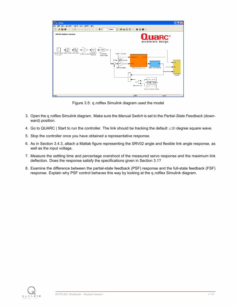
Figure 3.5: q rotflex Simulink diagram used the model

3. Open the q rotflex Simulink diagram. Make sure theManual Switch is set to the Partial-State Feedback (down-ward) position.

4. Go to QUARC | Start to run the controller. The link should be tracking the default ±20 degree square wave.

5. Stop the controller once you have obtained a representative response.

6. As in Section 3.4.3, attach a Matlab figure representing the SRV02 angle and flexible link angle response, aswell as the input voltage.

7. Measure the settling time and percentage overshoot of the measured servo response and the maximum linkdeflection. Does the response satisfy the specifications given in Section 3.1?

8. Examine the difference between the partial-state feedback (PSF) response and the full-state feedback (FSF)response. Explain why PSF control behaves this way by looking at the q rotflex Simulink diagram.


3.5 Results

Fill out Table 2 with your answers from your control lab results - both simulation and implementation.

Description Symbol Value UnitsPre Lab QuestionsDesired poles DPCompanion Gain KSimulation: Control Design

Transformation Matrix W

Control Gain KClosed-loop poles CLPSimulation: Closed-Loop SystemMaximum deflection |α|max degMaximum voltage |Vm|max VImplementationControl Gain KMaximum deflection |α|max degMaximum voltage |Vm|max V

Table 2: Results


4 SYSTEM REQUIREMENTSRequired Software

• Microsoft Visual Studio

• Matlabrwith Simulinkr, Real-Time Workshop, and the Control System Toolbox.

• QUARCr2.1, or later.

See the QUARCrsoftware compatibility chart at [6] to see what versions of MS VS and Matlab are compatible withyour version of QUARC and for what OS.

Required Hardware

• Data-acquisition (DAQ) card that is compatible with QUARC. This includes Quanser Hardware-in-the-loop(HIL) boards such as:

– Q2-USB– Q8-USB– QPID– QPIDe

and some National Instruments DAQ devices (e.g., NI USB-6251, NI PCIe-6259). For a full listing of compliantDAQ cards, see Reference [2].

• Quanser SRV02-ET rotary servo.

• Quanser Rotary Flexible Joint (attached to SRV02).

• Quanser VoltPAQ-X1 power amplifier, or equivalent.

Before Starting Lab

Before you begin this laboratory make sure:

• QUARCris installed on your PC, as described in [4].

• The QUARC Analog Loopback Demo has been ran successfully.

• SRV02 Rotary Flexible Joint and amplifier are connected to your DAQ board as described Reference [8].


4.1 Overview of Files

File Name DescriptionFlexible Joint User Manual.pdf This manual describes the hardware of the Rotary Flexi-

ble Joint system and explains how to setup and wire thesystem for the experiments.

Flexible Joint Workbook (Student).pdf This laboratory guide contains pre-lab questions and labexperiments demonstrating how to design and implementa position controller on the Quanser SRV02 Flexible Jointplant using QUARCr .

setup rotflex.m The main Matlab script that sets the SRV02 motor andsensor parameters, the SRV02 configuration-dependentmodel parameters, and the Flexible Joint (i.e., rotflex) sen-sor parameters. Run this file only to setup the laboratory.

config srv02.m Returns the configuration-based SRV02 model specifica-tions Rm, kt, km, Kg, eta g, Beq, Jeq, and eta m, thesensor calibration constants K POT, K ENC, and K TACH,and the amplifier limits VMAX AMP and IMAX AMP.

config rotflex.m Returns the Flexible Joint model inertia, Jl, and viscousdamping, Bl.

ROTFLEX ABCD eqns student.m Contains the incomplete state-space A, B, C, and D ma-trices. These are used to represent the Flexible Joint sys-tem.

calc conversion constants.m Returns various conversions factors.d pole placement student.m Use this script to find the feedback control gain K.s rotflex.mdl Simulink file that simulates the Flexible Joint system when

using a full or partial state-feedback control.q rotflex id.mdl When ran with QUARCr, this Simulink model feed a Sine

Sweep signal to the servo and measures the correspond-ing Flexible Joint angle. The measured response can thenbe used to find the natural frequency of the link.

q rotflex val.mdl This Simulink model is used with QUARCrto compare theFlexible Joint state-space model with the measured re-sponse from the actual system.

q rotflex.mdl Simulink file that implements a closed-loop state-feedbackcontroller on the actual ROTFLEX system using QUARCr

.

Table 3: Files supplied with the SRV02 Flexible Joint Control Laboratory.

4.2 Setup for Finding Stiffness

Before beginning in-lab procedure outlined in Section 2.3.1, the q rotflex id Simulink diagram must be properlyconfigured.

Follow these steps:

1. Setup the SRV02 with the Flexible Joint module as detailed in the Flexible Joint User Manual ([7]).

2. Load the Matlab software.

3. Browse through theCurrent Directory window in Matlab and find the folder that contains the file q rotflex id.mdl.

4. Open the q rotflex id.mdl Simulink diagram, shown in Figure 2.4.


5. Configure DAQ: Ensure the HIL Initialize block subsystem is configured for the DAQ device that is installedin your system. By default, the block is setup for the Quanser Q8 hardware-in-the-loop board. See Reference[2] for more information on configuring the HIL Initialize block.

4.3 Setup for Model Validation

Before performing the in-lab exercises in Section 2.3.2, the q rotflex val Simulink diagram and the setup rotflex.mscript must be configured.

Follow these steps to get the system ready for this lab:

1. Setup the SRV02 with the Flexible Joint module as detailed in [7].


3. Browse through theCurrent Directory window in Matlab and find the folder that contains the QUARCROTFLEXfile q rotflex val.mdl.

4. Open the q rotflex val.mdl Simulink diagram, shown in Figure 2.6.

5. Configure DAQ: Ensure the HIL Initialize block in the SRV02 Flexible Joint subsystem is configured for theDAQ device that is installed in your system. By default, the block is setup for the Quanser Q8 hardware-in-the-loop board. See Reference [2] for more information on configuring the HIL Initialize block.

6. Configure Sensor: The position of the SRV02 load shaft can be measured using either the potentiometer orthe encoder. Set the Pos Src Source block in q rotflex val, as shown in Figure 2.6, as follows:

• 1 to use the potentiometer• 2 to use to the encoder

Note that when using the potentiometer, there will be a discontinuity.

7. Configure Input: Set theManual Switch to the DOWN position for a step input or the UP position for a squaresignal.

8. Open the setup rotflex.m file. This is the setup script used for the ROTFLEX Simulink models.

9. Configure setup script: When used with the Flexible Joint, the SRV02 has no load (i.e., no disc or bar) andhas to be in the high-gear configuration. Make sure the script is setup to match this setup:

• EXT GEAR CONFIG to 'HIGH'• LOAD TYPE to 'NONE'• Ensure ENCODER TYPE, TACH OPTION, K CABLE, AMP TYPE, and VMAX DAC parameters are setaccording to the SRV02 system that is to be used in the laboratory.

• CONTROL TYPE to 'MANUAL'.

4.4 Setup for Flexible Joint Control Simulation

Before going through the control simulation in Section 3.4.2, the s rotflex Simulink diagram and the setup rotflex.mscript must be configured.

Follow these steps to configure the lab properly:


2. IMPORTANT:Make sure themodel you found in Section 2.3.2 is entered in ROTFLEX ABCD eqns student.m.


3. Browse through the Current Directory window in Matlab and find the folder that contains the s rotflex.mdl file.

4. Open s rotflex.mdl Simulink diagram shown in Figure 3.3.

5. Configure the setup rotflex.m script according to your hardware. See Section 4.3 for more information.

6. Run the setup rotflex.m script.

7. Enter the stiffness (Ks) you found in Section 2.3.1.

4.5 Setup for Flexible Joint Control Implementa-tion

Before beginning the in-lab exercises given in Section 3.4.3 (or Section 3.4.4), the q rotflex Simulink diagram andthe setup rotflex.m script must be setup.

Follow these steps to get the system ready for this lab:

1. Setup the SRV02 with the Flexible Joint module as detailed in [7] .


3. Browse through the Current Directory window in Matlab and find the folder that contains the q rotflex.mdl file.

4. Open the q rotflex.mdl Simulink diagram shown in Figure 3.5.

5. Configure DAQ: Ensure the HIL Initialize block in the SRV02 Flexible Joint subsystem is configured for theDAQ device that is installed in your system. By default, the block is setup for the Quanser Q8 hardware-in-the-loop board. See Reference [2] for more information on configuring the HIL Initialize block.

6. Configure Sensor: The position of the SRV02 load shaft can be measured using the potentiometer or theencoder. Set the Pos Src Source block in q rotflex, as shown in Figure 3.5, as follows:

• 1 to use the potentiometer• 2 to use to the encoder

Note that when using the potentiometer, there will be a discontinuity.

7. Configure setup script: Set the parameters in the setup rotflex.m script according to your system setup. SeeSection 4.3 for more details.

8. Run the setup rotflex.m script.


5 LAB REPORTThis laboratory contains two groups of experiments, namely,

1. Modeling the Quanser Rotary Flexible Joint system, and

2. State-feedback control.

For each experiment, follow the outline corresponding to that experiment to build the content of your report. Also,in Section 5.3 you can find some basic tips for the format of your report.

5.1 Template for Content (Modeling)

I. PROCEDURE

1. Finding Stiffness

• Briefly describe the main goal of the experiment.• Briefly describe the experiment procedure in Step 3 in Section 2.3.1.

2. Model Validation

• Briefly describe the main goal of the experiment.• Briefly describe loading the model in Step 6 in Section 2.3.2.• Briefly describe the model validation experiment in Step 13 in Section 2.3.2.

II. RESULTS

Do not interpret or analyze the data in this section. Just provide the results.

1. Frequency-response plot from step 3 in Section 2.3.1.

2. Model validation plot from step 13 in Section 2.3.2.

3. Provide applicable data collected in this laboratory (from Table 1).

III. ANALYSISProvide details of your calculations (methods used) for analysis for each of the following:

1. Measured link stiffness in step 6 in Section 2.3.1.

2. Model discrepancies given in step 15 in Section 2.3.2.

IV. CONCLUSIONSInterpret your results to arrive at logical conclusions for the following:

1. How does the model compare with the actual system in step 14 of Section 2.3.2, State-space model validation.


5.2 Template for Content (Control)

I. PROCEDURE

1. Control Design

• Briefly describe the main goal of the control design.• Briefly describe the control design procedure in Step 3 in Section 3.4.1.

2. Simulation

• Briefly describe the main goal of the simulation.• Briefly describe the simulation procedure in Step 3 in Section 3.4.2.

3. Full-State Feedback Implementation

• Briefly describe the main goal of this experiment.• Briefly describe the experimental procedure in Step 7 in Section 3.4.3.

4. Partial-State Feedback Implementation

• Briefly describe the main goal of this experiment.• Briefly describe the experimental procedure in Step 6 in Section 3.4.4.

II. RESULTSDo not interpret or analyze the data in this section. Just provide the results.

1. Matrices from Step 3 in Section 3.4.1, Find transformation matrix.

2. Response plot from step 3 in Section 3.4.2, Full-state feedback controller simulation.

3. Response plot from step 7 in Section 3.4.3, for Full-state feedback controller implementation.

4. Response plot from step 6 in Section 3.4.4, for Partial-state feedback controller implementation.

5. Provide applicable data collected in this laboratory (from Table 2).

III. ANALYSISProvide details of your calculations (methods used) for analysis for each of the following:

1. Controllability of system in Step 2 in Section 3.4.1.

2. Closed-loop poles in Step 5 in Section 3.4.1.

3. Matlab commands used to generate the control gain in Step 6 in Section 3.4.1.

4. Settling time, percent overshoot, link deflection, and input voltage Step 4 in Section 3.4.2, Full-state feedbackcontroller simulation.

5. Settling time, percent overshoot, link deflection, and input voltage in Step 8 in Section 3.4.3, Full-state feedbackcontroller implementation.

6. Settling time, percent overshoot, link deflection, and input voltage in Step 7 in Section 3.4.3, Partial-statefeedback controller implementation.

7. Comparison between partial-state and full-state feedback in step 8 in Section 3.4.4.

IV. CONCLUSIONSInterpret your results to arrive at logical conclusions for the following:


1. Whether the closed-loop poles are in the required location in Step 5 in Section 3.4.1.

2. Whether the controller meets the specifications in Step 4 in Section 3.4.2, Full-state feedback controller simu-lation.

3. Whether the controller meets the specifications in Step 8 in Section 3.4.3, for Full-state feedback controllerimplementation.

4. Whether the controller meets the specifications in Step 7 in Section 3.4.4, for Partial-state feedback controllerimplementation.


5.3 Tips for Report Format

PROFESSIONAL APPEARANCE

• Has cover page with all necessary details (title, course, student name(s), etc.)

• Each of the required sections is completed (Procedure, Results, Analysis and Conclusions).

• Typed.

• All grammar/spelling correct.

• Report layout is neat.

• Does not exceed specified maximum page limit, if any.

• Pages are numbered.

• Equations are consecutively numbered.

• Figures are numbered, axes have labels, each figure has a descriptive caption.

• Tables are numbered, they include labels, each table has a descriptive caption.

• Data are presented in a useful format (graphs, numerical, table, charts, diagrams).

• No hand drawn sketches/diagrams.

• References are cited using correct format.


REFERENCES[1] Bruce Francis. Ece1619 linear systems course notes (university of toronto), 2001.

[2] Quanser Inc. QUARC User Manual.

[3] Quanser Inc. SRV02 QUARC Integration, 2008.

[4] Quanser Inc. QUARC Installation Guide, 2009.

[5] Quanser Inc. SRV02 User Manual, 2009.

[6] Quanser Inc. QUARC Compatibility Table, 2010.

[7] Quanser Inc. SRV02 Rotary Flexible Joint User Manual, 2011.

[8] Quanser Inc. SRV02 Rotary Flexible Link User Manual, 2011.

[9] B. P. Lathi. Modern Digital and Analog Communication Systems. Oxford University Press, Inc., 3rd edition,1998.

[10] Norman S. Nise. Control Systems Engineering. John Wiley & Sons, Inc., 2008.


USER MANUALSRV02 Rotary Servo Base Unit

Set Up and Configuration

Developed by:Jacob Apkarian, Ph.D., QuanserMichel Lévis, M.A.Sc., Quanser

Hakan Gurocak, Ph.D., Washington State University

CAptiVAtE. MotiVAtE. GRAdUAtE. Solutions for teaching and research. Made in Canada.

[email protected] +1-905-940-3575 QUANSER.CoM

ten modules to teach controls from the basic to advanced level

SRV02 Base Unit Flexible Link inverted pendulum

Ball and Beam

Multi-doF torsion2 doF inverted pendulum

2 doF Robot

Flexible Joint Gyro/Stable platform

double inverted pendulum

2 doF Ball Balancer

With the SRV02 Base Unit, you can select from 10 add-on modules to create experiments of varying complexity across a wide range of topics, disciplines and courses. All of the experiments/workstations are compatible with LabVIEW™ and MATLAB®/Simulink®.

To request a demonstration or a quote, please email [email protected].

©2011 Quanser Inc. All rights reserved. LabVIEW™ is a trademark of National Instruments. MATLAB® and Simulink® are registered trademarks of The MathWorks, Inc.

Quanser educational solutions are powered by:

Documents

Ten modules to teach controls from the basic to advanced