Temporary Investment Tax Incentives: Theory with …shapiro/papers/aer2008.pdf · I. Temporary Investment Tax Incentives: ... This choice of units leads to a particularly transparent

737

American Economic Review 2008, 98:3, 737–768http://www.aeaweb.org/articles.php?doi=10.1257/aer.98.3.737

Even modest reductions in the after-tax cost of capital purchases provide strong incentives for increased investment. Indeed, for tax subsidies that are temporary, and for capital goods that are very long-lived, the incentive to invest when the after-tax price is temporarily low is essentially infinite. Firms that would have purchased new capital equipment in the future, instead make their purchases during the period of the subsidy. For tax increases, the effects are the opposite. Firms, that would have normally invested now, delay until the tax rate returns to normal.

We present a model of the equilibrium effects of temporary investment tax incentives. The model reveals a simple relationship between the shadow price of investment goods and the size of a temporary investment tax incentive. Specifically, for sufficiently long-lived capital goods (goods with very low rates of economic depreciation) and for sufficiently short-lived investment tax subsidies, the shadow value of capital should be nearly unchanged, and thus the pre-tax shadow price of capital goods should fully reflect the magnitude of the tax subsidy. This result holds regardless of the elasticity of investment supply and regardless of the underlying demand for capital. Instead, it relies only on the firm’s ability to arbitrage predictable movements in the after-tax price of long-lived capital over time. Two conclusions immediately follow. First, observ-ing price increases following a temporary tax incentive is not evidence that investment supply is relatively inelastic. A temporary investment tax subsidy can substantially affect investment even if it bids up the price of investment sharply. Second, because economic theory dictates that the shadow price of investment moves one-for-one with a temporary tax subsidy, the elasticity of supply can be inferred from quantity data alone.

Recent changes in US tax law allow us to use the model and its implications to estimate struc-tural parameters that govern the supply of investment. The 2002 and 2003 tax bills provided temporarily accelerated tax depreciation called bonus depreciation for certain types of qualified capital goods. Under the 2002 bill, firms could immediately deduct 30 percent of investment purchases and then depreciate the remaining 70 percent under standard depreciation schedules.

Temporary Investment Tax Incentives: Theory with Evidence from Bonus Depreciation

By Christopher L. House and Matthew D. Shapiro*

The intertemporal elasticity of investment for long-lived capital goods is nearly infinite. Consequently, investment prices should fully reflect temporary tax sub-sidies, regardless of the investment supply elasticity. Since prices move one-for-one with the subsidy, elasticities can be inferred from quantities alone. This paper uses a recent tax policy—bonus depreciation—to estimate the invest-ment supply elasticity. Investment in qualified capital increased sharply. The estimated elasticity is high—between 6 and 14. There is no evidence that mar-ket prices reacted to the subsidy, suggesting that adjustment costs are internal, or that measurement error masks the price changes. (JEL G31, H32)

* House: Department of Economics, University of Michigan, Ann Arbor, MI 48109, and National Bureau of Eco-nomic Research (e-mail: [email protected]); Shapiro: Department of Economics, University of Michigan, Ann Arbor, MI 48109, and National Bureau of Economic Research (e-mail: [email protected]). The authors gratefully acknowl-edge the comments of William Gale, Austan Goolsbee, Yuriy Gorodnichenko, James Hines, Peter Orszag, Samara Potter, Dan Silverman, Joel Slemrod, seminar participants, and anonymous referees.

JunE 2008738 THE AMERICAn ECOnOMIC REVIEW

Under the 2003 bill, the immediate deduction increased to 50 percent. This investment subsidy was explicitly temporary. Only investments made through the end of 2004 qualified for this tax treatment. Moreover, the subsidy applied differentially to different types of capital. Our empiri-cal research design examines disaggregate investment data in the wake of these tax provisions. The temporary nature of the subsidy, together with the differential treatment of types of capital goods, provide a natural experiment that fits precisely into our analytical framework.

We use the model to estimate the elasticity of supply for investment goods. The data clearly show that the policy had a substantial stimulative impact on investment in capital goods that ben-efited most from bonus depreciation. Our estimates of the elasticity of supply are high—roughly between 6 and 14. Market prices, on the other hand, show little if any tendency to increase in the short run. The absence of a price change suggests that either the price data are too noisy to detect the effect of the tax subsidy, or that internal adjustment costs (investment adjustment costs not reflected in the market price) played a significant role in containing investment demand.

Section I presents the model used in our analysis, shows some general results for temporary investment tax incentives, and discusses their econometric implications. Section II describes the tax changes in the 2002 and 2003 laws and extends the model to analyze these provisions. Section III estimates the structural parameters of our model using the variation in the data from the policy changes. Section IV offers our conclusions.

I. Temporary Investment Tax Incentives: Theory

In this section we present the model that we use to analyze temporary investment tax subsidies. The model allows for a general type of investment subsidy. In Section II, we modify the model to consider the specific bonus depreciation allowances included in the 2002 and 2003 tax bills. We use the model to present some basic properties of temporary investment tax subsidies and to moti-vate our empirical research design. The model yields a precise econometric relationship that we exploit to estimate key structural parameters governing the effects of tax policy on investment.

A. Model

Firms demand capital goods for use in production. Because the tax policies we analyze pro-vide different incentives for different types of capital goods, we include several different types of capital in the model. Let m 5 1, … , M be an index of capital types. For each type m, let dm be the economic rate of depreciation, and let K m be the stock of capital. Let F 1K 1t , K

2t , … , Kt

M 2 be a representative firm’s production function measured in terms of units of a numeraire good.1 Capital income is taxed twice—once as business profit and again when capital income is distrib-uted to the owners of the firm. The tax rate on profit is represented by tp, and the tax rate on the distribution of capital income (dividends and capital gains taxes) by t d.

The firm chooses K mt11 and Itm to maximize the present discounted value of profits

(1) a`

j50 Gt1j e 11 2 t dt1j 2 11 2 tp

t1j 2 F (K 1t1j , K 2t1j , … , K Mt1j 2 2 aM

m 51 wm

t1j I mt1j 11 2 z mt1j 2 f ,

subject to the constraints

(2) K mt11 5 K tm 11 2 dm 2 1 I t

m, for all m.

1 Because they do not influence the analysis, we suppress labor and other inputs in the production function.

VOL. 98 nO. 3 739HOuSE And SHApIRO: TEMpORARy InVESTMEnT TAx InCEnTIVES

Here, wtm is the real relative price of type m capital and I t

m is gross investment in type m capital. The variable z t

m is the total effective subsidy on new purchases of type m capital including the value of depreciation deductions and any investment tax credits. Gt1j is the discounted value of real profits at time t 1 j. The usual specification would take Gt1j 5 b ju9 1Ct1j 2 / u9 1Ct 2 , where u9 1Ct 2 is the marginal utility of consumption at date t, and would thus measure the discounted sum in units of the date t numeraire good. We instead choose Gt1j 5 b ju9 1Ct1j 2 . Of course, mul-tiplying each term in a present value by a common positive number does not change the solution of the maximization problem; rather, it changes only the units of the objective. Our choice of Gt1j means that the shadow value on constraint (2) is in units of utility rather than in units of date t goods. This choice of units leads to a particularly transparent analysis of temporary policies.

The firm’s optimization requires the first-order conditions

(3) q tm 5 bu9 1Ct112 c 11 2 t pt112 11 2 t dt11 2 'F

'K mt11

d 1 b 11 2 d m 2 q mt11

and

(4) qtm 5 u9 1Ct 2 wt

m 31 2 ztm 4

for all m. The variable qtm, the Lagrange multiplier on constraint (2), is the shadow value of an

additional unit of type m capital. Equation (3) is the first-order condition for the choice of K mt11 and equation (4) is the first-order condition for the choice of I t

m. Equation (4) relates the shadow value of capital qt

m to the pre-tax shadow price of capital w mt . Again, our normalization of (1) implies that these Lagrange multipliers are in units of utility. Note also that qt

m is not Brainard-Tobin’s Q. If adjustment costs were external, Q for type m capital would be qt

m / 1u9 1Ct 2 w tm 2 .

Below, we argue that in response to temporary tax policies, movements in qtm are negligible. In

contrast, Brainard-Tobin’s Q will move in response to temporary tax policies because these poli-cies typically affect investment goods prices and the marginal utility of consumption.

The supply of new capital goods is governed by a type-specific supply curve. We denote these supply curves as w m 1I tm 2 , reflecting the assumption that the pre-tax marginal cost of type m capital goods w t

m is a function of the quantity of type m investment I tm. The prices are measured

in terms of units of the consumption numeraire. We assume that the marginal cost functions are increasing. For our empirical analysis, we specify that the supply functions are given by

(5) w m 1I tm 2 5 1I tm/ I m 2 11/j 2 ,

where I m is the steady-state level of investment for type m capital. Thus, the elasticity of supply is j, and the steady-state real relative price is one.2

The real prices wtm (the marginal costs of producing additional investment) can have two dif-

ferent interpretations. First, they could be interpreted as external costs. External costs corre-spond to the marginal cost of production at capital-producing firms and are therefore typically reflected in the purchase price of investment goods. Second, they could be interpreted as internal adjustment costs. Internal costs (e.g., Hayashi 1982) could arise due to disruption and congestion within the firm caused by investment activity. Internal adjustment costs are not reflected in the

2 Our functional form differs from that of Fumio Hayashi (1982), which requires zero-degree homogeneity in the investment/capital ratio. Holding the capital stock fixed, one can show that, if g is the adjustment cost parameter in the Hayashi form 1 i.e., g 5 dQ / d 1I / K 2 2 , then our elasticity is j 5 (g d)21

.


measured purchase price of the investment goods (Michael L. Mussa 1977). While this distinc-tion is not important for the economic decisions made by the firm (i.e., conditions (3) and (4) will hold in either case), it is important for measurement and econometric interpretation.

B. Short-Run Approximations for Long-Lived Investment Goods

We now present some fundamental properties of temporary investment tax incentives. This analysis sheds light on the basic economic incentives involved in such policies and motivates our empirical analysis of the 2002 and 2003 investment policies.

Suppose the government credibly announces a temporary investment tax subsidy. The tax subsidy temporarily increases zt

m for certain (perhaps all) investment goods. The precise form of the subsidy is not important at this point; it could be an investment tax credit, a bonus deprecia-tion allowance, etc.

Although the model is complicated, two short-run approximations yield sharp, analytical results about the effects of temporary investment subsidies. The accuracy of these approxima-tions rests on two conditions. First, the policy must be temporary. Second, the investment goods in question must be long-lived investment goods, that is, goods with low economic rates of depre-ciation. The approximations are less accurate and potentially quite misleading for long-lasting changes in policy or for capital that depreciates rapidly.

The exact solution to the model is complicated because it has both backward- and forward-looking variables. For sufficiently temporary tax changes, however, it is a good approximation to replace the forward-looking variables qt

m , and the backward-looking variables Ktm, with their

associated steady-state values, q m and K m. Replacing the capital stock with its steady-state value is standard in many settings. The stock of long-lived capital is much bigger than the flow, and thus changes only slightly in the short run. Specifically, the percent change in the capital stock is approximately d m times the percent change in investment.

The justification for approximating qtm with its steady-state value is more subtle. Expanding

equation (3), we can write qtm as

(6) qtm 5 ba

`

j50 eu9 1Ct1j112 3 b 11 2 d m 2 4 j c 11 2 t pt1j112 11 2 t dt1j112 'F

'Kmt1j11

d f .

Because the policy change is temporary, the system will eventually return to its steady state. While this may take some time, most of the terms in the brackets, particularly those in the future, remain close to their steady-state values. Put differently, the difference between qt

m and its steady-state level q m comes entirely from the first several terms in the expansion—the short-run terms. Provided that the firm is sufficiently patient (i.e., b is close to 1) and that depreciation is sufficiently slow (i.e., d m is close to 0), the future terms dominate this expression and the short-run behavior of the system has only minor influences on qt

m.This approximation has a natural economic interpretation. The decision to invest is inherently

forward-looking. As such, the benefits from investment are anchored by future, long-run consid-erations. As long as the far future is only mildly influenced by temporary policies, the benefit to any given investment is largely independent of short-run considerations.

C. Response of Investment to Temporary Tax Subsidies

We now analyze the equilibrium response of the price and quantity of investment goods to temporary tax subsidies. Conventional supply and demand reasoning can be misleading because


capital is durable and therefore subject to a stock demand. Expectations about the future domi-nate current investment decisions. Our analysis should come as no surprise to careful readers of Dale W. Jorgenson (1963), Andrew B. Abel (1982), Lawrence H. Summers (1987), or, indeed, of Robert E. Lucas’s (1976) critique, which took “investment demand” as an example. To dem-onstrate how misleading conventional supply and demand reasoning can be, we show that in response to a temporary tax subsidy, the shadow price of investment goods moves one-for-one with the investment subsidy, regardless of the elasticity of investment supply. This result has important econometric implications.

In the model, equation (5) gives the real pre-tax price of new type m capital wtm, which includes

all costs of investment (internal plus external). Figure 1 plots this equation for a single type of capital. The total pre-tax price of investment wt

m is on the vertical axis and the quantity of invest-ment It

m is on the horizontal axis. The slope of this curve is governed by the elasticity j.Equation (4) relates the shadow price of capital wt

m to its shadow value qtm, the marginal util-

ity of resources u9 1Ct 2 , and the tax subsidy ztm. Using our short-run approximation, qt

m < q m, we have an equation relating the pre-tax price of investment goods to the tax subsidy and the marginal utility of consumption. This equation does not involve the rate of investment. Plotting equation (4) gives a horizontal line with shift variables Ct and zt

m.The equilibrium price and rate of investment for each m is determined by the intersection of

(4) and (5). Because qtm < q m, the price can be recovered from (4) alone,

(7) wtm <

q mu r 1Ct 21 2 zt

m ,

which is independent of both the elasticity of supply and the quantity of investment. If the policy does not change aggregate consumption, then, as shown in Figure 1, the shadow price of capital changes one-for-one with the subsidy. If the policy does have aggregate effects, all shadow prices move depending on the change in the marginal utility of consumption. In this case, changes in the relative pre-tax shadow prices for different types of investment goods fully reflect any differ-ences in tax subsidies (the relative after-tax shadow prices are unchanged).3 Thus, for temporary tax subsidies, the pre-tax price of long-lived investment goods should fully reflect the tax sub-sidy, regardless of the rate at which the marginal cost of investment rises.

If the marginal utility of consumption is isoelastic and additively separable, then there is an exact log-linear relationship between investment, consumption, and the tax subsidy. Let u9 1Ct 2 5 Ct

21/s where s is the elasticity of intertemporal substitution for consumption. Let dvt denote the deviation of a variable vt from its steady-state value n and let v t be the percent deviation of vt from its steady-state value, that is, dvt 5 vt 2 v and v t ; dvt /v. Then, using the constancy of qt

m under a temporary tax subsidy, equations (4) and (5) imply that

(8) Itm 5

j

1 2 zm d ztm 1

j

s C

t ,

where d ztm is a change in the investment subsidy from its steady-state value zm. If the tax subsidy

has no aggregate effects, C t 5 0, so the elasticity of investment supply j can be inferred directly

from the change in investment. General equilibrium effects influence investment through the overall scarcity of resources. Because we can use observed consumption to control for this

3 This finding has antecedents in the Q-theoretical investment literature. Abel (1982) shows that an instantaneous, tem-porary tax change has no effect on after-tax Q (which he calls q* ). Since after-tax Q is constant, pre-tax Q fully reflects the policy change. (See also Hayashi 1982; Summers 1981, 1987; and Alan J. Auerbach and James R. Hines 1987.)


general equilibrium effect, there is no need to specify or simulate the entire model to estimate the parameters.

Equation (8) indicates that when the subsidy expires, investment will simply return to its steady-state value. The fundamental value of the good 1qt

m 2 is unchanged by the transitory policy and, thus, investment returns to normal in the absence of the subsidy. This implication runs counter to the intuition that investment would be abnormally low immediately following the expiration of the subsidy. While it is true that subsidized investment effectively substitutes for future investment, the reduction in future investment is spread out over a long period of time.

The derivation of equations (7) and (8) requires very few assumptions. Among other things, the derivation requires no reference to the production function F, the marginal product of capital, or the supply and demand of other productive inputs. All that is required is a stable supply curve (equation (5) in our model), and the assumption that the investment is long-lived and that the policy is sufficiently temporary. Because the structural relationships do not require many strong assumptions, the theoretical conclusions, which form the basis for our econometric analysis, hold without having to specify restrictive auxiliary conditions. Of course, the structural estimates of the supply elasticity depend on the form of the supply function. Below we return to the issue of functional form.

D. Accuracy of the Approximation

The approximations qt < q and Kt < K are exactly true only for either arbitrarily short-lived policies or for arbitrarily low depreciation rates (and discount rates). For realistic policy dura-tions and for real world depreciation rates, these approximations are not exact. To evaluate the accuracy of our approximations, we present a simple example of the approximation for a variety of depreciation rates and policy durations. For simplicity, we focus on a single type of capital. We take the production function to be AKt

a with a 5 0.35. We hold the marginal utility of con-sumption constant. We assume that r 5 0.02 (annually), which requires b 5 0.98. The supply of investment is given by equation (5).

Table 1 presents the equilibrium change in the shadow price of capital goods w in response to an investment tax subsidy of 1 percent 1dz 5 0.012 . Our approximation says that the change in the price w should be 1 percent (or, equivalently, that the change in the shadow value q should be zero).

ItI0

t

I1 I1

1

0

Figure 1. Price and Quantity Responses to Temporary Investment Subsidies


Consider a long-lived capital good with an annual depreciation rate of 2 percent (comparable to many structures). If the elasticity of supply is 1.00 and the subsidy lasts for one year, the price rises by 0.993 percent. The change in the shadow value (not reported) is simply the difference between the subsidy and the price change. Thus, the percent change in q for this case is 20.007 percent. For higher elasticities, the approximation deteriorates. If j 5 10, the change in w is 0.954 percent. As the discussion above suggests, the approximation is best for very temporary policies or very long-lived durables. Moreover, that the approximation does not hold for longer-duration policies with capital that depreciates rapidly is exactly what the theory predicts.4

Table 1 abstracts from general equilibrium movements in interest rates, employment, and so on. In the earlier working paper version of this article (House and Shapiro 2006b), we ana-lyzed the general equilibrium effects of the policy. Because the bonus depreciation allowance was so narrowly targeted, the aggregate effects of the policy were quite modest. These general

4 Table 1 was generated with a real interest rate of 2 percent. Versions of the same table with 4 and 6 percent interest rates produced results that were almost identical. For instance, with a 6 percent interest rate, for d 5 0.02, and j 5 1, the price change for a policy lasting one year is 0.991 percent instead of 0.993 percent.

Table 1—Response to a Temporary Investment Subsidy

DurationDepreciation

rate

Shadow price 1w 2j 5 0 j 5 0.5 j 5 1 j 5 5 j 5 10 j 5 15 j 5 20

6 months d 5 0.001 1.000 1.000 1.000 0.999 0.998 0.997 0.996d 5 0.01 1.000 0.999 0.998 0.992 0.986 0.982 0.978d 5 0.02 1.000 0.998 0.996 0.986 0.976 0.969 0.963d 5 0.05 1.000 0.996 0.992 0.970 0.951 0.936 0.923d 5 0.10 1.000 0.992 0.985 0.945 0.911 0.885 0.864d 5 0.25 1.000 0.982 0.965 0.877 0.807 0.755 0.714

1 year d 5 0.001 1.000 1.000 0.999 0.997 0.995 0.993 0.991d 5 0.01 1.000 0.998 0.996 0.983 0.972 0.964 0.956d 5 0.02 1.000 0.996 0.993 0.972 0.954 0.940 0.928d 5 0.05 1.000 0.992 0.984 0.941 0.906 0.878 0.855d 5 0.10 1.000 0.985 0.971 0.896 0.835 0.790 0.753d 5 0.25 1.000 0.966 0.936 0.784 0.673 0.597 0.539

2 years d 5 0.001 1.000 0.999 0.999 0.995 0.990 0.986 0.983d 5 0.01 1.000 0.996 0.992 0.967 0.946 0.930 0.915d 5 0.02 1.000 0.992 0.985 0.946 0.912 0.886 0.864d 5 0.05 1.000 0.984 0.969 0.890 0.826 0.779 0.740d 5 0.10 1.000 0.971 0.946 0.814 0.715 0.645 0.591d 5 0.25 1.000 0.941 0.891 0.659 0.515 0.428 0.368

3 years d 5 0.001 1.000 0.999 0.998 0.992 0.985 0.980 0.975d 5 0.01 1.000 0.993 0.988 0.952 0.922 0.898 0.878d 5 0.02 1.000 0.989 0.979 0.921 0.873 0.837 0.807d 5 0.05 1.000 0.976 0.956 0.845 0.760 0.698 0.649d 5 0.10 1.000 0.959 0.925 0.749 0.626 0.545 0.485d 5 0.25 1.000 0.922 0.860 0.587 0.439 0.357 0.304

Permanent d 5 0.001 1.000 0.986 0.972 0.884 0.806 0.749 0.704d 5 0.01 1.000 0.929 0.872 0.637 0.513 0.443 0.396d 5 0.02 1.000 0.908 0.839 0.578 0.453 0.387 0.343d 5 0.05 1.000 0.888 0.808 0.528 0.405 0.341 0.300d 5 0.10 1.000 0.879 0.794 0.506 0.384 0.322 0.282d 5 0.25 1.000 0.872 0.783 0.489 0.367 0.306 0.267

notes: The table shows the equilibrium percent change in the shadow price of capital goods w in response to an invest-ment subsidy of 1 percent 1dz 5 0.012 . Investment supply is given by equation (5). For the numerical calculations, the production function is AKt

a, r 5 0.02, and a 5 0.35.


equilibrium effects would slightly attenuate the pass-through of the subsidy to prices shown in Table 1 by causing consumers to substitute away from nondurable consumption and into subsi-dized investment.5

E. Implications for Observed prices

Price increases are a necessary accompaniment of a temporary investment subsidy. Observing increased investment goods prices following a temporary tax subsidy is not necessarily evidence of a relatively inelastic supply curve. Theory implies that the pre-tax price should rise roughly one-for-one with the investment subsidy regardless of the elasticity of supply. Because theory has such sharp implications for the equilibrium determination of prices, it is useful to consider what conclusions, if any, could be drawn from price data.

Recall that the shadow price of investment goods reflects both external and internal marginal costs of new investment. External adjustment costs arise due to rising marginal costs of produc-tion at capital producing firms, and should therefore be reflected in the measured purchase price of investment goods. Internal adjustment costs arise due to disruption and congestion and, since they are simply absorbed by the purchasing firm, are not reflected in the purchase price. This distinction does not matter for the determination of investment, but it does matter for relating the predictions of the model to observations in the data, which capture only market (i.e., external) prices. Let pt

m be the market price of type m investment goods. We assume that internal adjust-ment costs are zero in steady state and that changes in the shadow cost are a reflection of changes in external and internal adjustment costs. If u is the fraction of external adjustment costs,

(9) ptm 5 1 1 u 1wt

m 2 12 .

Movements in the shadow price affect market prices only to the extent that adjustment cost are external to the firm. If u were one so that all investment adjustment costs were external, then we could test neoclassical investment theory by observing whether prices increased one-for-one with a temporary tax subsidy. Alternatively, price data can be used to estimate u.

II. Bonus Depreciation

We use the temporary bonus depreciation allowances provided in the 2002 and 2003 tax bills to estimate the elasticity of investment supply. In this section we describe the normal treatment of depreciation in the US Tax Code, as well as the temporary incentives provided by the 2002 and 2003 laws. We then extend our model to include a bonus depreciation allowance like the one in the laws. Our aim is to re-derive equation (8) for the special case of bonus depreciation. The analysis provides the econometric relationships that we use in Section III.

A. The Modified Accelerated Cost Recovery System

When a firm invests in new capital, it deducts the purchase price of the investment from its taxable income. In most cases, the firm cannot deduct the entire amount immediately. Instead, the firm makes a sequence of deductions for depreciation over a specified period of time. Under US law, the schedule of depreciation deductions is specified by the Modified Accelerated Cost

5 While their aggregate effects were probably modest, the 2002 and 2003 bonus depreciation policies had noticeable effects on the economy. For the US economy as a whole, these policies may have increased GDP by $10 to $20 billion and may have been responsible for the creation of 100,000 to 200,000 jobs.


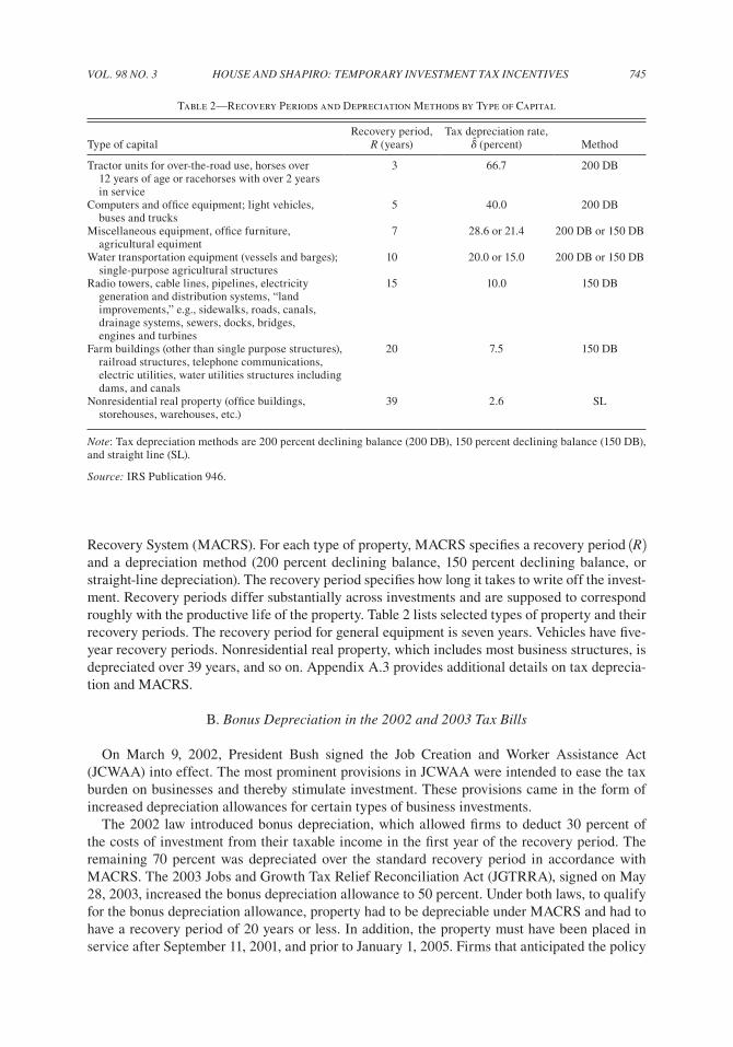
Recovery System (MACRS). For each type of property, MACRS specifies a recovery period 1R2 and a depreciation method (200 percent declining balance, 150 percent declining balance, or straight-line depreciation). The recovery period specifies how long it takes to write off the invest-ment. Recovery periods differ substantially across investments and are supposed to correspond roughly with the productive life of the property. Table 2 lists selected types of property and their recovery periods. The recovery period for general equipment is seven years. Vehicles have five-year recovery periods. Nonresidential real property, which includes most business structures, is depreciated over 39 years, and so on. Appendix A.3 provides additional details on tax deprecia-tion and MACRS.

B. Bonus depreciation in the 2002 and 2003 Tax Bills

On March 9, 2002, President Bush signed the Job Creation and Worker Assistance Act (JCWAA) into effect. The most prominent provisions in JCWAA were intended to ease the tax burden on businesses and thereby stimulate investment. These provisions came in the form of increased depreciation allowances for certain types of business investments.

The 2002 law introduced bonus depreciation, which allowed firms to deduct 30 percent of the costs of investment from their taxable income in the first year of the recovery period. The remaining 70 percent was depreciated over the standard recovery period in accordance with MACRS. The 2003 Jobs and Growth Tax Relief Reconciliation Act (JGTRRA), signed on May 28, 2003, increased the bonus depreciation allowance to 50 percent. Under both laws, to qualify for the bonus depreciation allowance, property had to be depreciable under MACRS and had to have a recovery period of 20 years or less. In addition, the property must have been placed in service after September 11, 2001, and prior to January 1, 2005. Firms that anticipated the policy

Table 2—Recovery Periods and Depreciation Methods by Type of Capital

Type of capitalRecovery period,

R (years)Tax depreciation rate,

d (percent) Method

Tractor units for over-the-road use, horses over 12 years of age or racehorses with over 2 years in service

3 66.7 200 DB

Computers and office equipment; light vehicles, buses and trucks

5 40.0 200 DB

Miscellaneous equipment, office furniture, agricultural equiment

7 28.6 or 21.4 200 DB or 150 DB

Water transportation equipment (vessels and barges); single-purpose agricultural structures

10 20.0 or 15.0 200 DB or 150 DB

Radio towers, cable lines, pipelines, electricity generation and distribution systems, “land improvements,” e.g., sidewalks, roads, canals, drainage systems, sewers, docks, bridges, engines and turbines

15 10.0 150 DB

Farm buildings (other than single purpose structures), railroad structures, telephone communications, electric utilities, water utilities structures including dams, and canals

20 7.5 150 DB

Nonresidential real property (office buildings, storehouses, warehouses, etc.)

39 2.6 SL

note: Tax depreciation methods are 200 percent declining balance (200 DB), 150 percent declining balance (150 DB), and straight line (SL).

Source: IRS Publication 946.


would rationally increase investment in the third quarter in 2001.6 We return to the issue of the timing of the policy when we present our results.

Both the 2002 and 2003 laws included additional investment incentives targeted specifically at small businesses.7 Prior to JCWAA, the US tax system allowed firms to expense investment up to $24,000 annually under Section 179 of the tax code. The 2002 law increased this limit to $25,000. The 2003 law increased the Section 179 exemption to $100,000 through the end of 2005. Like the bonus depreciation allowance, this exemption applied only to property with a recovery period of no more than 20 years. We return to the issue of Section 179 in Section IIID.

C. Modeling Accelerated and Bonus depreciation

Robert E. Hall and Jorgenson (1967) analyze depreciation allowances by assuming that the firm immediately recovers the present discounted value of depreciation deductions when it invests. Let dj

m be the schedule of depreciation deductions for type m capital. The steady-state present discounted value of these deductions z m is

(10) z m 5 aR

j51

Djm

11 1 p 2 j 11 1 r2 j ,

where p is the rate of inflation and r is the real interest rate. Inflation reduces the value of z m because tax depreciation allowances are not indexed for inflation.

Let l tm denote a bonus depreciation allowance for type m capital. As in the 2002 and 2003

legislation, for every dollar of investment in such capital, firms write off l tm immediately and

the remaining 11 2 l tm 2 is depreciated according to the usual depreciation schedule. The present

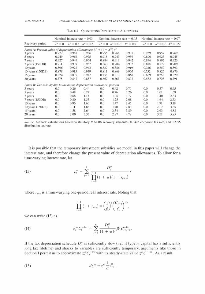
value of depreciation allowances with the bonus is l tm 1 11 2 l t

m 2 z m. Table 3, Panel A reports the present discounted value of depreciation deductions l t

m 1 11 2 l tm 2 z m for various MACRS

recovery periods and various nominal interest rates 1approximately r 1 p2 . The subsidy for investment in type m capital zt

m is then

(11) ztm 5 11 2 td 2 tp 1l t

m 1 11 2 l tm 2 z m).

Table 3, panel B, shows the percent change in the after-tax price due to the bonus depreciation, that is,

(12) dzt

m

1 2 zm 5 11 2 td 2tp 11 2 zm 21 2 11 2 td 2tpzm l t

m ,

where we have used dl tm 5 l t

m at steady-state lm 5 0. (Recall that variables without time subscripts are steady-state values.) For property with very short recovery periods, the investment subsidy is small. For five-year property, the 50 percent bonus depreciation reduces the cost of investment by 1.26 percent with a 5 percent nominal interest rate. For longer recovery periods, the bonus is worth more. Note that 20-year properties get a subsidy of roughly 5 percent with the 50 percent bonus depreciation deduction.8

6 JCWAA requires that the property be acquired (but not necessarily placed in service) before September 11, 2004. JGTRRA eliminated this requirement.

7 The bills also had other provisions. Because these provisions do not have strong effects across types of capital, we do not analyze them in this paper. For an analysis of the income tax provisions of the 2001 and 2003 tax policies, see House and Shapiro (2006a).

8 For the subsidy to be effective, firms must pay at least some income tax. As long as they pay some tax, the value of the subsidy is independent of capital structure.


It is possible that the temporary investment subsidies we model in this paper will change the interest rate, and therefore change the present value of depreciation allowances. To allow for a time-varying interest rate, let

(13) z tm 5 a

R

j51

D j

m

qj21

s5011 1 p 2 11 1 rt1s 2

,

where rt1s is a time-varying one-period real interest rate. Noting that

qj21

s50 11 1 rt1s 2 5 a1

bb

j

aCt1 j

Ctb

1/s

,

we can write (13) as

(14) z tm

Ct21/s 5 a

R

j51

D jm

11 1 p 2 j b j Ct1

21/j11

s .

If the tax depreciation schedule djm is sufficiently slow (i.e., if type m capital has a sufficiently

long tax lifetime) and shocks to variables are sufficiently temporary, arguments like those in Section I permit us to approximate z t

mCt21/s with its steady-state value z mC21/s . As a result,

(15) dz tm < z m

1s

C t .

Table 3—Quantifying Depreciation Allowances

Nominal interest rate 5 0.03 Nominal interest rate 5 0.05 Nominal interest rate 5 0.07

Recovery period lm 5 0 lm 5 0.3 lm 5 0.5 lm 5 0 lm 5 0.3 lm 5 0.5 lm 5 0 lm 5 0.3 lm 5 0.5

panel A: present value of depreciation allowances: lm 1 11 2 lm 2 z m

3 years 0.972 0.981 0.986 0.955 0.968 0.977 0.939 0.957 0.9695 years 0.949 0.964 0.975 0.918 0.943 0.959 0.890 0.923 0.9457 years 0.927 0.949 0.964 0.884 0.919 0.942 0.846 0.892 0.9237 years (150DB) 0.914 0.939 0.957 0.863 0.904 0.932 0.818 0.872 0.90910 years 0.896 0.927 0.948 0.837 0.886 0.919 0.786 0.850 0.89310 years (150DB) 0.878 0.915 0.939 0.811 0.868 0.905 0.752 0.826 0.87615 years 0.824 0.877 0.912 0.733 0.813 0.867 0.659 0.761 0.82920 years 0.775 0.842 0.887 0.667 0.767 0.833 0.582 0.708 0.791

panel B: Tax subsidy due to the bonus depreciation allowance, percent3 years 0.0 0.26 0.44 0.0 0.42 0.70 0.0 0.57 0.955 years 0.0 0.48 0.79 0.0 0.76 1.26 0.0 1.01 1.697 years 0.0 0.68 1.13 0.0 1.06 1.77 0.0 1.40 2.337 years (150DB) 0.0 0.80 1.33 0.0 1.25 2.08 0.0 1.64 2.7310 years 0.0 0.96 1.60 0.0 1.47 2.45 0.0 1.91 3.1810 years (150DB) 0.0 1.11 1.86 0.0 1.70 2.83 0.0 2.19 3.6515 years 0.0 1.58 2.64 0.0 2.34 3.89 0.0 2.93 4.8820 years 0.0 2.00 3.33 0.0 2.87 4.78 0.0 3.51 5.85

Source: Authors’ calculations based on statutory MACRS recovery schedules, 0.3425 corporate tax rate, and 0.2975 distribution tax rate.


Totally differentiating (11) gives the change in the tax subsidy from implementing bonus depre-ciation, so

(16) dztm 5 11 2 t d 2 tp 1 11 2 z m 2 l t

m 1 dz tm 2 .

We can now write the general relationship between investment and a temporary investment tax subsidy derived in Section I in terms of the bonus depreciation allowance. Substituting (15) into (16), we can write (8) as

(17) I tm 5 j atp 11 2 td 2 11 2 zm 2

1 2 tp 11 2 td 2zm b l tm 1 aj

sb a 1

1 2 tp 11 2 td 2zmb C t .

The first term is the direct change in investment due to bonus depreciation. The second term reflects any aggregate effects of the policy and includes both changes in the aggregate scarcity of resources and changes in the value of depreciation allowances caused by changes in interest rates.

The real relative prices of investment goods are also affected by the policy. Because w tm 5

11/j 2 I tm, the pre-tax shadow price of type m capital is

(18) w tm 5 atp 11 2 td 2 11 2 zm 2

1 2 tp 11 2 td 2zm b l tm 1 a1

sb a 1

1 2 tp 11 2 td 2zmb C t .

As in Section I, this equation is independent of the elasticity of supply j. The first term is the discounted value of the tax subsidy itself. In the absence of changes in C

t, the shadow price of investment goods increases one-for-one with the tax subsidy.

Equations (17) and (18) can be used to illustrate the predicted effects of bonus depreciation. Figure 2 plots deviations in investment and real relative prices implied by (17) and (18) against the tax depreciation rates for ten different types of capital goods for the quarters immediately after the legislation: 2002:II and 2003:III. The tax depreciation rates 1d m 2 are a convenient way to summarize the tax treatment of the different types of capital. We calculate tax depreciation rates simply by dividing the declining balance rate (either 200, 150, or 100) by the recovery period. The resulting d m is a constant geometric rate that approximates the statutory depreciation schedule dj

m. See Table 2 and Appendix A.2 for specific values of d m. To generate the figures, we chose parameter values for tp and t d and calculated z m for each type of capital according to the approximate MACRS tax depreciation rates. We set C

t to zero in each time period. We used the bonus depreciation rates l t

m provided by the law and set j to 9, which is roughly the midpoint of the estimates we get in the next section. In Figure 2, each point represents the percent deviation from steady state of a particular type of capital. Solid circles indicate capital types that qualify for bonus depreciation. Empty circles indicate capital types that do not qualify.

The top panels of Figure 2 show the changes in real investment spending immediately after the 2002 and 2003 laws go into effect. Capital goods with the lowest tax depreciation rates do not qualify for bonus depreciation and thus experience no change in investment. Investment jumps up sharply for 20-year property and 15-year property, the qualified capital with the low-est tax depreciation rates (d m of 7.5 percent and 10.0 percent, respectively). These long-lived properties experience the greatest benefit from the bonus. Since the tax subsidy decreases as the tax depreciation rate increases, investment in qualified capital declines steadily as a function of tax depreciation rates. The lower panels graph the changes in real shadow prices against the tax depreciation rates. The response is the same as for quantity except for scaling by the elasticity of supply.


The cross-sectional differences in the tax treatment play a central role in our empirical analy-sis. The 20- and 15-year properties get the greatest subsidies. Referring back to Table 2, the heavily subsidized goods include, among other things, radio towers, cable lines, electricity dis-tribution systems, land improvements (sidewalks, etc.), railroad structures, telephone commu-nications towers, electric utilities, and water utilities. These goods are long-lived, but are not structures in the usual sense. We refer to these investment goods as “quasi-structures,” since they share features of both equipment and structures. Loosely speaking, the empirical analysis in the next section compares investment in these quasi-structures with investment in short-lived capi-tal (e.g., vehicles, computers, general equipment, and so forth, which have five- and seven-year recovery periods) and in long-lived capital goods that do not qualify (structures).

III. Empirical Analysis of Bonus Depreciation

We use data on real investment spending and real investment prices to estimate the param-eters of equations (17) and (18). The estimates yield a value for the elasticity of supply (j) and allow us to test whether investment prices reflect the tax subsidy. The structural interpretation

Figure 2. Simulated Response to Bonus Depreciation Policy

notes: Simulated response of investment (top panels) and shadow prices (lower panels) for various types of capital to the 30 percent (2002:II) and 50 percent (2003:III) bonus depreciation policy. The approximate geometric tax depre-ciation rate 1dm 2 is on the horizontal axis. Percent deviation from steady state is on the vertical axis. Each circle corre-sponds to approximate response to bonus depreciation based on equations (17) and (18). Solid circles are for capital that qualifies for bonus depreciation. Empty circles represent unqualified capital. In the upper panels, j 5 9.


of our estimates leans heavily on two key conditions. First, for the tax changes we study and the investment goods we observe, we need the limiting approximations qt

m < q m to hold. Second, we require that the supply side of the market is correctly specified. In particular, we assume that each type of investment good is governed by a stable supply function as described in equation (5).

A. data

We use data from the Bureau of Economic Analysis (BEA) to construct a quarterly panel of investment quantities and prices by type. We match the BEA investment data to Internal Revenue Service (IRS) depreciation schedules. Once we exclude BEA types that do not have clear matches to the IRS depreciation schedules, our panel has 36 types of capital with quarterly observations from 1959:I to 2006:IV. We construct real investment purchases by dividing nominal purchases of type m capital by the price index for that type. The relative price for type m capital is defined as the mth price index divided by the price index for nondurable consumption from the National Income and Product Accounts (NIPA). (Appendix A.2 provides more information on these data. See Table A.2 for a complete list of the capital goods in our dataset.) To construct z m for each type, we use actual MACRS depreciation schedules (see IRS Publication 946) and an annual nominal interest rate of 5 percent. Equations (17) and (18) require data on the tax rates tp and t d, and data on the cyclical component of aggregate consumption C

t . We set tp 5 0.3425 and t d 5 0.2975. (For details on the calculation of these tax rates, see Appendix A.1.) For the aggregate consumption series C

t, we use HP-filtered real consumption of nondurables with a quarterly smoothing parameter of 1,600. Our econometric procedure also requires aggregate data on GDP and corporate profits and data on type-specific investment tax credits (ITC).9

B. Econometric Specification and Estimation

Equations (17) and (18) show how investment quantities and prices respond to bonus deprecia-tion. Before turning our attention to these structural equations, we first need to estimate what investment and prices would have been in the absence of the policy. We use several decades of data prior to the policy to forecast investment quantities and prices for each type of capital. The resulting forecast errors measure deviations in investment and prices. These forecast errors serve as data for the structural equations (17) and (18). Of course, the deviations from steady state also reflect the response of investment quantity and price to many shocks other than the bonus depreciation policy. As long as these other factors are uncorrelated with the differential impact of bonus depreciation by type of capital, our estimation procedure gives valid results.

The forecasting equations we use to project investment quantity and price are reduced forms. Our theory does not mandate what variables to include in the forecasting equations. Our aim is simply to control for major determinants of investment quantities and prices unrelated to the policy we are studying. We construct forecasts for horizons h 5 1, … , H using forecasting equa-tions of the form

(19) ln 1Itm1h 2 5 BI

h, m X tm 1 eI, t

h, m

and

(20) ln 1 ptm1h 2 5 Bp

h, m X tm 1 ep, t

h, m.

9 We are grateful to Dale Jorgenson for providing us with the data on the ITC by capital type.


Itm1h and pt

m1h are the investment quantity and price for horizon h and type m capital. The vector

X tm includes the variables we use to construct the forecasts. BI

h, m and Bph, m are the corresponding

parameters. Since (19) and (20) are simply auxiliary forecasting equations, we are fairly agnostic about their specification. Our baseline specification for the forecast equations includes the t and t 2 1 values of the following variables: type-specific investment quantities and prices, the log of aggregate real GDP, the corporate profit rate, and the type-specific investment tax credit. It also includes a constant and a time trend.

Our procedure simply requires unbiased estimates of what investment would have been without the policy change. To check the sensitivity of our estimates to the specification of the forecasting equations, we consider two alternative specifications. First, as a parsimonious alternative, we use forecasting equations with only a constant and a time trend in X t

m. Second, we consider a speci-fication that, like the baseline specification, uses lagged information on type-specific investment, prices, and the ITC, but unlike the baseline uses contemporaneous data on aggregate GDP and corporate profits in the forecasting equations.

We estimate (19) and (20) over the sample period t 5 1, … , T 5 1965:I to 2000:IV. We then use these equations to project investment quantities and prices over 2001:I to 2006:IV. Because our forecasts for this period all condition on the same information (i.e., information at date t 5 2000:IV), we can suppress the subscript t and write the forecast errors as e I

h,m for investment and e p

h,m for prices. Each h 5 1, … , H corresponds to a quarter between 2001:I and 2006:IV (h 5 1 is 2001:1).

We estimate (17) and (18) with the forecast errors as the left-hand-side variables. Define C1m

and C2m as

C1m 5

tp 11 2 td 2 11 2 zm 21 2 tp 11 2 td 2zm and C2

m 5 1

1 2 tp 11 2 td 2zm .

These parameters are constant across time, but differ across types of capital m. Calculating C1m

and C2m requires values for t p, t d, and z m which are observable. Referring back to equation (17),

our model implies

(21) e Ih,m 5 bI0 1 jlh

m C1m 1

j

s C2

m C h 1 eI

h, m,

where bI0 , j, and j/s are parameters to be estimated, and eIh,m is an error unrelated to the change

in the policy. The bonus rate lhm is 0.3 or 0.5 for eligible capital during 2002:II to 2004:I and zero

otherwise, that is, lhm 5 0 for ineligible capital and for all capital prior to 2002:II and after 2004:

IV. The corresponding version of (18) is

(22) e ph, m 5 bp0 1 bp1C1

m lhm 1

1s

C2m C

h 1 eph, m.

If investment adjustment costs were entirely external (and thus included in measured prices), the estimate of bp1 should be one. Since adjustment costs may be partially internal, any value of bp1 between zero and one is consistent with the theory.

At a fundamental level, variation in tax policy across types and across time identifies the struc-tural parameters in the model. Investment is also influenced by aggregate conditions. Equations (21) and (22) show that the response to aggregate conditions varies systematically across the type of capital. According to the model, the appropriate control variable is marginal utility times C2

m. To control for aggregate conditions, we consider two measures of marginal utility. First, we use the parametric specification u9 1Ct 2 5 Ct

21/s. For this case, marginal utility is proportional to C h


(HP-filtered consumption of nondurables). Thus, our first specification includes C2m C

h as a con-trol variable. Our second specification allows for the possibility that marginal utility is poorly-proxied by filtered consumption. We replace the consumption-based measure of marginal utility with time-dummies scaled by the same type-specific factors. That is, in the second specification of equation (21), the term js21 C2

m C h is replaced by gH

k51 bk C2m d h, k, where bk are parameters

that subsume js21 C k and d h, k 5 1 if h 5 k and zero otherwise (i.e., d h, k are time-dummy

variables). We make a similar substitution for equation (22). These estimates treat the marginal utility of consumption as an unobserved time-varying object that is common across investment types. Obviously, using time-dummies, the parameter s is not identified.

The disturbances eIh,m and ep

h,m are not independently distributed. Within type, the forecast errors are likely correlated across time. There is also substantial heteroskedacity across types because some types of investment are less predictable than others. Finally, there is correlation across types because certain investment goods react to common shocks in a systematic way. We estimate (21) and (22) by ordinary least squares (OLS) and also by weighted least squares (WLS), which weigh each observation according to the precision of its first-stage estimates. The WLS estimates improve the efficiency of the structural estimates in light of the strong heteroskedacity in the forecast errors across types. Appendix A.4 describes our estimation procedure in greater detail.

C. Results

Scatterplots.—Before turning to the structural estimates of (21) and (22), it is instructive to plot the data. Figure 3 shows the forecast errors from the baseline forecast specification. Each panel represents a time period. The tax depreciation rates are on the horizontal axes. The panels on the top row show the forecast errors for real investment, while the lower panels show the fore-cast errors for real relative prices. These plots correspond to the theoretical plots shown in Figure 2. Each point in the figure is the forecast error for a single quarter and a single type of capital. Since each panel includes multiple quarters, there are several observations per type. Solid points are types that qualify for bonus depreciation. Empty circles are types that do not qualify. We group the data into five time periods. The first period, 2001:I to 2001:III, was before the policy was discussed or in effect. The second period, 2001:IV to 2002:I, was before the policy was law but during which the policy applied retroactively. We refer to the second period as the anticipa-tion period. The third and fourth periods, 2002:II to 2003:II, and 2003:III to 2004:IV correspond to the periods of the 30 and 50 percent bonus. The last period, 2005:I to 2006:IV is after the policy expired.

Consider the data for investment quantity shown in the top row of Figure 3. As one would expect, in the first period (before the policy), there is no discernable relationship between the tax depreciation rate and investment forecast errors. In the anticipation period, the pattern predicted by the theory is clearly evident. There is a sharp discontinuity between eligible property and ineligible property, and there is a negative relationship between the tax depreciation rate and investment among qualified properties. This pattern remains in the third and fourth panels. In the fifth panel, after the expiration of the policy, the data do not clearly return to normal. The nega-tive relationship among qualified types is not clear, but the discontinuity between unqualified types and qualified types with low tax depreciation rates persists into the 2005–2006 period.

Overall, comparing the actual forecast errors for real investment in Figure 3 with the simu-lated data in Figure 2 suggests that the tax policy had the predicted effects. Below, we discuss the expiration of the policy in 2005.

The bottom row of Figure 3 shows the same plots for the price data. Unlike the quantity data, there is no discernable pattern of price movements across types of capital or across time periods.


The variability in the forecast errors suggests that it is not going to be possible to test the theory using these data. We confirm this below in the econometric analysis.

Structural Estimates of Elasticity of Supply.—We now turn to the structural estimates of equa-tions (21) and (22). We fit these equations with the data plotted in Figure 3. The left-hand-side variables are the forecast errors, and the explanatory variables are as defined in the equations. For these estimates, the timing of the policy corresponds to the signing dates and the expiration date provided by the law. Thus, the 30 percent bonus goes into effect in 2002:II, the 50 percent bonus goes into effect in 2003:III, and the policy expires in 2005:I.

Table 4 shows the estimates of the structural parameters. Panel A gives the estimates of the investment equation (21). The rows present alternative econometric specifications of the forecast-ing and structural equations. Rows 1–3 present estimates using the baseline second-stage regres-sion with HP-filtered consumption as a measure of marginal utility. Rows 4–6 present estimates using estimated time-dummies for the marginal utility of consumption. The rows also differ in the specification of the first-stage forecasting equations (19) and (20). Rows 1 and 4 use the base-line forecast specification. Rows 2 and 5 use only time trends to forecast investment. Rows 3 and 6

Figure 3. Forecast Errors for Real Investment and Real Prices

notes: The figure plots forecast errors for real investment (upper panels) and real investment prices (lower panels) by type of capital. The forecast errors come from the baseline forecasting equations (19) and (20). Solid circles are for capital that qualify for bonus depreciation. Empty circles are unqualified capital. The tax depreciation rate 1dm 2 is on the horizontal axis.


use type-specific data on lagged investment quantities and prices but, unlike the baseline, use contemporaneous information on GDP and corporate profits to control for possible differences in the systematic cyclical behavior of investment across types.

In the first row of panel A, the baseline forecast specification, the WLS estimate of j is 7.68 with an adjusted standard error of 1.85. The OLS point estimate is similar, but with a somewhat larger standard error. Since the OLS and WLS estimates are similar for all specifications, we dis-cuss only the more efficient WLS estimates. As expected, the standard errors in the specification with only a time trend (row 2) are larger because the forecasts are less precise and thus there is more noise in the data used in the second stage. Row 3, which uses contemporaneous aggregate variables in the first stage, gives an estimate of j of 6.13. It is worth noticing that the estimates of j/s (in columns 3 and 4) are all higher than the estimates of j, suggesting that the intertemporal elasticity of substitution for consumption is less than one.

Table 4—Structural Parameter Estimates

j j/s

Row First stage Second stage WLS OLS WLS OLS

panel A: Investment equation 12121 Baseline Baseline 7.68 7.03 14.41 10.04

11.852 12.672 12.792 15.7722 Time trend only Baseline 6.31 7.09 13.89 14.58

13.662 15.872 15.272 18.7323 Contemporaneous Baseline 6.13 4.61 12.53 10.95

aggregate variables 11.792 12.532 12.622 15.1824 Baseline Time-varying 14.82 11.74 n.a. n.a.

Mu 1C 2 13.072 13.602 n.a. n.a.5 Time trend only Time-varying 13.83 13.78 n.a. n.a.

Mu 1C 2 15.932 18.342 n.a. n.a.6 Contemporaneous Time-varying 13.21 9.60 n.a. n.a.

aggregate variables Mu 1C 2 12.962 13.392 n.a. n.a.

bp, 1 1/s

Row First stage Second stage WLS OLS WLS OLS

panel B: price equation 12221 Baseline Baseline 21.07 20.92 0.37 0.18

11.552 11.632 13.502 14.5122 Time trend only Baseline 20.86 20.30 20.31 20.03

10.992 11.382 12.182 12.1523 Contemporaneous Baseline 20.56 20.48 1.31 20.64

aggregate variables 11.692 11.782 13.882 14.8124 Baseline Time-varying 20.76 20.57 n.a. n.a.

Mu 1C 2 11.732 11.982 n.a. n.a.5 Time trend only Time-varying 20.75 0.13 n.a. n.a.

Mu 1C 2 11.172 12.072 n.a. n.a.6 Contemporaneous Time-varying 20.97 20.83 n.a. n.a.

aggregate variables Mu 1C 2 11.872 12.152 n.a. n.a.

notes: The baseline forecast specification (rows 1 and 4) includes a constant, trend, two lags of real GDP, real cor-porate profits, type-specific real investment, type-specific real relative prices, and type-specific ITC. The trend-only forecast specification (rows 2 and 5) includes only a constant and trend. The first-stage specification with contempo-raneous aggregate variables is identical to the baseline forecast specification, except that date t data for GDP and cor-porate profits are used to forecast date t investment. The baseline structural specification (rows 1–3) uses HP-filtered consumption to measure aggregate marginal utility. The time-varying Mu 1C 2 specification (rows 4–6) uses time dum-mies. Estimates are by ordinary least squares (OLS) or weighted least squares (WLS). Standard errors in parentheses are corrected for time-series and cross-sectional dependence. See text and Appendix A.4 for details.


Rows 4–6 of panel A give the estimates for the specification where the scaled time-dummies replace the consumption-based measure of marginal utility as the control for the aggregate effects of the policy. The point estimates for j are uniformly higher than the estimates from the specification using the consumption-based measure of marginal utility. Roughly speaking, these estimates are twice as high as the estimates in rows 1–3 1j is 14.82 in the baseline forecast specification).

The econometric estimates quantify what was evident from Figure 3. There is a powerful response of the quantity of investment to the bonus for types of capital that benefited substan-tially from the bonus. The strong movements in quantity yield high estimates of the elasticity of supply—ranging between 6 and 14.

Structural Estimates of Implied Bonus Rate.—In the estimation presented in Table 4, l hm is

a known parameter of the tax policy—equal to 0.3 or 0.5 for eligible capital during the period of the bonus, and zero otherwise. The exact timing of the bonus in these estimates is assumed to match the enactment in law, that is, zero prior to 2002:II and after 2004:IV. Alternatively, we can estimate the time series of the implied bonus rates that best fit the cross section of invest-ment period by period. To do so, we extend equation (21) to allow for a time-varying bonus rate. Specifically, we estimate

(23) e Ih,m 5 bI0 1 a

H

k 51 Lk j C1

m dh, k Bm 1

j

s C2

m C h 1 eI

h,m.

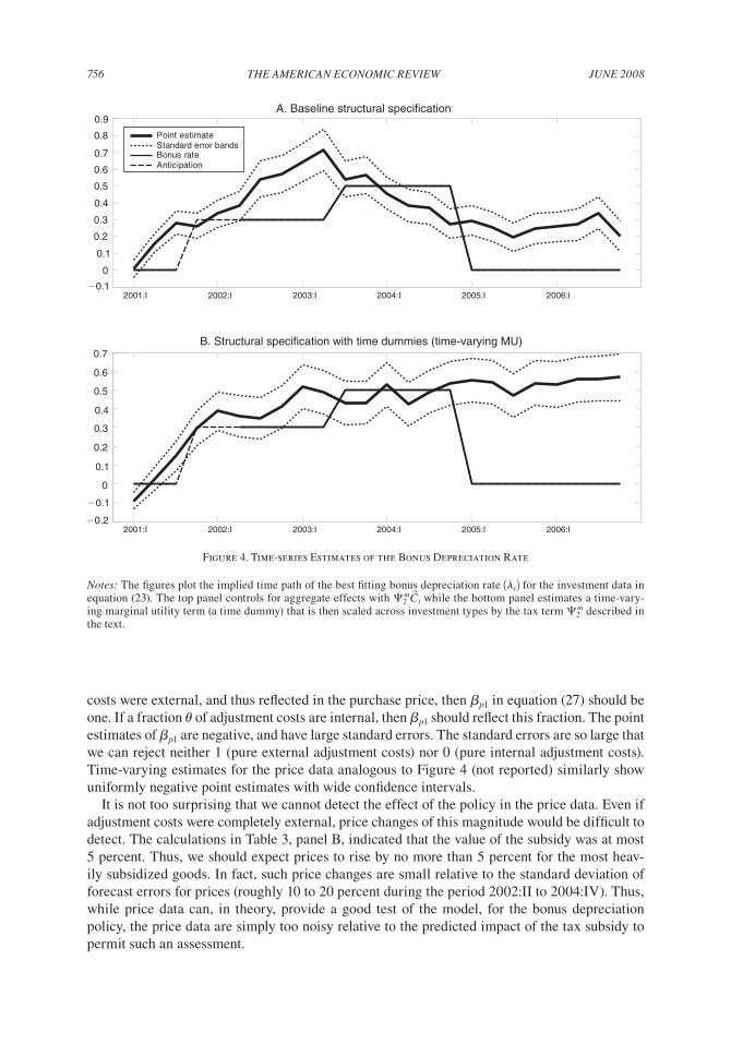
Here, Lk is the implied bonus rate for period k, and dh, k is, again, a time-dummy equal to one when h 5 k, and zero otherwise. Bm equals one for types eligible for the bonus, and zero other-wise. Since the implied bonus and the elasticity of supply cannot be identified separately, in equation (23) we set j at a fixed value of 14, roughly the upper bound on the estimates in Table 4. Figure 4 plots the estimates of Lh , the implied bonus rate. The dotted lines are one-standard-error bands. The thin solid line is the time path of the statutory bonus depreciation rate (dashed during the retroactive/anticipation period). As in Table 4, we consider specifications with either aggregate consumption (top panel) or scaled time-dummies (bottom panel) to control for aggre-gate effects. We use the baseline specification in the first stage for both panels of Figure 4.

The implied bonus rate in the upper panel of Figure 4 closely tracks the actual bonus rate. The estimates are close to zero in early 2001, but then jump in mid- to late 2001. This finding is con-sistent with a credible anticipation of the enactment of the retroactive policy. The implied bonus tapers off throughout 2003 and 2004. Empirically, this means that the differential increase in investment in types of goods benefiting most from the bonus is diminishing. By 2005, when the bonus has expired, the implied bonus is approaching zero.

The diminishing effect of the policy in the upper panel of Figure 4 is not clearly evident in the scatterplots in Figure 3. Indeed, when we reestimate (23) using C2

m-scaled time dummies instead of C2

m C t , the estimated effects of the policy persist throughout 2005 and 2006. The lower panel

of Figure 4 plots the implied bonus rate for this specification. Looking back to Figure 3, it is clear that the evidence for 2005 and 2006 is mixed. It is, therefore, not surprising that our estimates also yield mixed results on this point.

Structural Estimates of Response of Investment price.—We now turn briefly to the structural estimates for the response of observed investment prices to bonus depreciation. It is clear from the scatterplots in Figure 3 that the sharp pattern exhibited by the quantities is not present in the price data. Table 4, panel B, reports the structural estimates of equation (22). The theory implies that the shadow price of capital should change one-for-one with the tax subsidy. If all adjustment


costs were external, and thus reflected in the purchase price, then bp1 in equation (27) should be one. If a fraction u of adjustment costs are internal, then bp1 should reflect this fraction. The point estimates of bp1 are negative, and have large standard errors. The standard errors are so large that we can reject neither 1 (pure external adjustment costs) nor 0 (pure internal adjustment costs). Time-varying estimates for the price data analogous to Figure 4 (not reported) similarly show uniformly negative point estimates with wide confidence intervals.

It is not too surprising that we cannot detect the effect of the policy in the price data. Even if adjustment costs were completely external, price changes of this magnitude would be difficult to detect. The calculations in Table 3, panel B, indicated that the value of the subsidy was at most 5 percent. Thus, we should expect prices to rise by no more than 5 percent for the most heav-ily subsidized goods. In fact, such price changes are small relative to the standard deviation of forecast errors for prices (roughly 10 to 20 percent during the period 2002:II to 2004:IV). Thus, while price data can, in theory, provide a good test of the model, for the bonus depreciation policy, the price data are simply too noisy relative to the predicted impact of the tax subsidy to permit such an assessment.

Figure 4. Time-series Estimates of the Bonus Depreciation Rate

notes: The figures plot the implied time path of the best fitting bonus depreciation rate 1lt 2 for the investment data in equation (23). The top panel controls for aggregate effects with C2

mC t while the bottom panel estimates a time-vary-

ing marginal utility term (a time dummy) that is then scaled across investment types by the tax term C2m described in

the text.


It is likely that much of the observed variation in the price data is due to measurement error.10 Since the quantity data are constructed using the price data, they also have measurement error. Because investment quantities and prices are left-hand-side variables in (21) and (22), classical measurement error reduces the precision of the coefficient estimates, but does not introduce bias. Investment quantities respond by many times the value of the subsidy. Hence, we can estimate the supply elasticity with precision, even with substantial measurement error in the price indexes used to deflate the nominal quantities.

D. discussion

Timing of the policy and Timing of Investment.—Our research design uses two dimensions of variation in the data—the differential value of the bonus depreciation allowance across type, and the time-series variation of the policy. While the cross-sectional investment data strongly support basic predictions of the model, the evidence from the timing of the changes, though gen-erally supportive of the theory, is not as sharp. Indeed, it appears that investment reacted prior to the signing of the bill and that the expiration of the policy was not clear in the data. We deal with the anticipation and expiration of the policy in turn.

Our scatterplots and econometric analysis clearly show that the effects of bonus depreciation were evident prior to its enactment. While the law was not signed until March 2002, there were clear signals in the preceding months that such legislation would be passed. On October 24, 2001, the House passed a bill including the bonus depreciation provisions.11 It is standard to make changes in tax provisions retroactive because it is well understood that failing to do so creates incentives to delay economic activity. Usually, provisions are retroactive to the date a law is introduced, but in this case, Congress chose the symbolic date of September 11, 2001. The continuing slow recovery of the economy from the 2001 recession made the eventual passage of the legislation relatively certain.12 Hence, it seems reasonable that the apparent anticipation of the policy in 2001:IV and 2002:I is not a fluke of the data.

The expiration of bonus depreciation occurred on schedule at the end of 2004. Our evidence on the expiration is mixed. Neither the scatterplots in Figure 3 nor the time varying implied bonus rate in Figure 4 provides clear evidence of the expiration. Moreover, in the top panel of Figure 4, the implied bonus peaked well before the expiration of the policy. Several important factors likely contribute to the lack of sharp evidence for the expiration of the policy. First, many invest-ment projects benefiting most from bonus depreciation—radio towers, farm buildings, electricity distribution systems, telephone communication systems, etc.—likely require substantial time to build and may have long lead times. In recognition of the time needed to build complex pieces

10 The BEA cautions researchers that the quality of the type-specific investment data is “significantly less than that of the higher level aggregates in which they are included” (see http://www.bea.gov/national/nipaweb/nipa_under-lying/SelectTable.asp). The heterogeneity and complexity of many capital goods (particularly structures and quasi-structures) limits the accuracy of the price data. Moreover, these data are gathered from a variety of sources outside the BEA (mostly trade associations) that do not ascribe to official price measurement practices. In contrast, nominal data on investment spending for structures and quasi-structures are collected directly by the Census Bureau and are measured more accurately.

11 The depreciation provisions were the first items in the bill (see Joint Committee on Taxation, October 11, 2001). These provisions—including the retroactivity to September 11, 2001—survived intact from the Ways and Means Committee’s markup on October 12, 2001, to the bill as finally enacted.

12 “While it has gotten little attention, the so-called bonus depreciation is the one corporate tax break sure to become law.” Boston Globe (December 7, 2001, E1).


of equipment, the original tax bill permitted certain property to claim bonus depreciation as late as January 1, 2006.13

Second, projects that did not qualify for this extension needed to be installed by the end of 2004 to receive the bonus. Thus, many firms had an incentive to front-load the projects to avoid missing the deadline. Many investment projects requiring more than one year lead time were effectively not subsidized in 2004.

Third, the increased small-business exemptions under Section 179 undoubtedly influence our results. The increased Section 179 exemption shares many of the features of bonus depreciation and is equivalent to a 100 percent bonus depreciation on qualified investment up to the maximum deduction under Section 179.14 Prior to 2002, businesses could expense $24,000 of investment per year. The 2002 bill raised this ceiling temporarily to $25,000. This exemption, like bonus depreciation, was set to expire at the end of 2004. The 2003 bill increased the ceiling further to $100,000 and extended the expiration date to the end of 2005. The 2004 Working Families Tax Relief Act, approved by Congress in September 2004, extended the $100,000 Section 179 ceiling to the end of 2007.15 Thus, in our data, the average effective bonus rate exceeds the statutory rates of 30 or 50 percent that we assume in our structural estimation. Moreover, because Section 179 was extended, it likely obscures the expiration of the 50 percent bonus at the end of 2004.

In summary, the pattern of changes our theory predicts is clearly evident in the cross-sectional investment data and, consequently, our econometric model yields a high estimate for the elas-ticity of supply. On the other hand, complications in the timing of the expiration of the policy, the confounding differential expiration of the Section 179 expensing, and time-to-build of large projects make the time-series evidence less sharp.

Robustness and Interpretation of the Structural Estimates.—Our structural estimates depend both on the accuracy of the limiting approximations and on the structure of the model. This sec-tion explores the sensitivity of the structural estimates to deviations from the assumptions neces-sary to implement the theory and from the applicability of the theory to the bonus depreciation policy.

Temporal approximation. Our structural approach relies on the approximation qtm < qm.

Because temporary policy changes can last for several years, the approximation, which is exact only for the limiting case of an infinitely lived durable or an arbitrarily short-lived policy, will be imperfect. Table 1, which shows the exact equilibrium responses to a hypothetical temporary 1 percent ITC, quantifies the magnitude of the possible biases. Consider a one-year policy with d 5 0.02 and j 5 1. The exact equilibrium change in w is 0.993 rather than 1.000. Since the true elasticity is 1, the change in investment will be 0.993 percent and our estimate of the elasticity would be 0.993 rather than 1 (biased down). The bias gets worse for longer lived policies, higher d, and higher j. For a two-year policy, with d 5 0.10 and j 5 10, the exact equilibrium change in w is 0.715 rather than 1.000, and our estimate of j will be 7.15 rather than 10. We estimate elasticities in the range of 6 to 14. The typical economic rate of depreciation in our sample is

13 To qualify for the extended expiration date, the property had to have a recovery period of at least ten years, and either have a production period of at least two years, or cost more than $1 million and have a production period of at least one year.

14 Firms above the cutoff faced the 30 or 50 percent bonus rate. Like many features of the US tax code, however, the 179 exemption has a phase-out range above its exemption cutoff. Thus, firms that are just above the cutoff faced effec-tive bonus rates between 100 and 30 or 50 percent.

15 The 2004 bill also extended several other expiring provisions. The bonus depreciation allowance was not among the extensions. The extended provisions include the child tax credit, the 10 percent tax bracket, marriage penalty relief, and AMT relief, all of which were set to expire under pre-existing law.


below 0.10. Thus, judging from the example in Table 1, our estimates may be biased downward by perhaps as much as 10 to 15 percent of their true values (i.e., instead of an elasticity of 6, the true elasticity might be 6.9).

Constrained or myopic firms. The approximation itself was derived under the assumption that investment decisions were made by rational firms that were not constrained by credit market fric-tions or borrowing constraints, or other real world considerations. While such factors likely play a role in some investment decisions, they do not overturn the implications of our analysis. To see this, suppose that investment decisions are made by two groups of firms. The first group includes unconstrained, rational firms that react the way theory dictates. The second group includes firms whose investment decisions are governed by other factors (borrowing constrained firms, firms that are unaware of, or do not understand, the policy change, or firms that simply cannot change the timing of their investment projects for one reason or another). The unconstrained firms still arbitrage predictable movements in the after-tax price, despite the existence of the constrained firms. In equilibrium, provided that we are sufficiently close to the limiting case, the uncon-strained firms will invest to the point that the purchase price fully reflects the amount of the subsidy.

Identification and the form of the supply function. The central feature of our analysis is the near invariance of the shadow values of long-lived investment goods to temporary investment subsidies. The estimate of the supply elasticity also depends on the particular specification of the investment supply function. The elasticity j that we estimate parameterizes the marginal rate of transformation between consumption goods and investment goods. Additionally, our model imposes that this elasticity is the same across types.

Alternative specifications of the supply functions could require a reinterpretation of our results. For example, suppose that type-specific investment goods It

m are produced from general investment goods It, which are, in turn, produced from units of the consumption good. In this case, condition (4) would be

(24) qtm 5 Ct

21/s c tm pt

I 31 2 ztm

4 ,

where ptI is the marginal cost of converting units of consumption into the general investment

good It, and c tm is the marginal cost of converting It into the type-specific investment good I t

m. Thus, in terms of our earlier formulation, wt

m 5 c tm pt

I . If the marginal cost functions for both type-specific and general investment goods are isoelastic, then I t

m 5 jc tm and I t 5 vp

tI. Following

the arguments in Section I, the relationship between investment and the tax subsidy would be

(25) I tm 5

j

1 2 zm d ztm 1

j

s C

t 2 j

v I t .

Equation (25) differs from equation (8) in two ways. First, it includes a control for aggregate investment activity. Second, the elasticity j reflects the marginal rate of transformation between general and type-specific investment goods, rather than the marginal rate of transformation between consumption and type-specific investment goods. In our formulation, v is infinite, so the last term drops out. It would be a mistake to apply our estimate if v were finite. One could estimate an equation like (25) in our framework. For the case of bonus depreciation, however, where the key variation is across types, we would not expect v to be well identified.16

16 We thank an anonymous referee for suggesting this example.


We should emphasize that while changes in the structural specification of the supply side change the structural interpretation of our estimates, they do not affect the implication that prices should rise one for one with the tax subsidy. In the specification above, the price wt

m 5 ct

mptI (the number of units of the consumption good per unit of type m investment good) will rise

one for one with the subsidy dztm.

Expectations. Our structural estimates depend critically on the public’s belief that the poli-cies were in fact temporary. Given the history of US tax policy, it would not be unreasonable to suspect that the bonus would be extended by legislation subsequent to the 2002 bill. In fact, a National Association of Business Economics (NABE) survey in January 2004 found that 62 percent of business economists expected the policy to be extended. That some people may have anticipated that the provision would be extended is not necessarily problematic. As long as there was some probability that the policy would expire, firms still had a powerful incentive to invest prior to 2005.

Endogeneity of the policy. Finally, the policy was introduced when the economy was still recovering from the 2001 recession. Because the identification rests primarily on cross-sectional variation, the estimates are largely immune to biases arising from aggregate shocks. Moreover, we control for type-specific responses of investment to aggregate conditions—measured either by consumption or by time dummies. On the other hand, if the bonus were directed at specific types of investment that suffered disproportionately in the downturn, the estimates could be biased. There is no evidence that the bonus was targeted in this way.

E. Related Empirical Literature

In this section we discuss several papers closely related to our work. Our work follows a large literature starting with Hall and Jorgenson (1967) that uses tax changes to analyze invest-ment decisions.17 One strand of this literature, to which our paper contributes, uses changes in tax parameters arising from specific changes in tax laws. Auerbach and Hassett (1991) use an empirical procedure particularly similar to ours to study the change in the composition of invest-ment in the wake of the tax reform act of 1986. Like our approach, they use a two-step procedure to analyze data on different types of investment goods and find that tax changes caused large changes in investment.18

Our paper makes a distinct contribution to the literature quantifying the response of invest-ment to changes in tax laws. First, this paper develops an important but overlooked implication of the standard model of capital accumulation—namely, that the demand for investment is infinitely elastic in response to temporary tax changes. Second, the paper shows how to use this implication to estimate the elasticity of investment supply using temporary investment tax changes. While they depend critically on the near infinite elasticity of investment demand, our estimates are free from most other parametric restrictions, except for the form of investment supply itself. Finally, this paper uses a recent and unusual tax change—bonus depreciation—to produce estimates.

Goolsbee (1998) also examines whether supply-side conditions attenuate the effect of tax sub-sidies on investment. He uses changes in investment tax incentives to estimate the relationship between prices and investment subsidies. He finds that investment tax incentives cause sharp

17 See also, for example, Martin S. Feldstein (1982), Auerbach and Kevin A. Hassett (1992), Mihir A. Desai and Austan D. Goolsbee (2004), and Robert S. Chirinko, Steven M. Fazzari, and Andrew P. Meyer (1999).

18 Other studies exploiting tax law changes include Jorgenson and Kun-Young Yun (1990) and Jason Cummins, Kevin A. Hassett, and R. Glenn Hubbard (1994).


increases in prices, and concludes that the supply of investment is relatively inelastic. Our theory suggests an alternative interpretation in the case of temporary tax subsidies. Because the price elasticity of investment demand is essentially infinite for long-lived capital, prices must rise by exactly the amount of the investment subsidy, regardless of the supply elasticity. Thus, the magnitude of observed price changes in response to temporary subsidies conveys no information about the elasticity of supply. Goolsbee correctly calls attention to the importance of the supply of investment in attenuating the impact of investment tax subsidies. Nonetheless, one cannot make inferences about the supply side with data on investment goods prices alone. As we have emphasized, inferences about supply must use data on investment quantities.

Goolsbee’s empirical finding of substantial price increases contrasts with our data, which do not show a clear price reaction.19 Although we do not know exactly what is responsible for the discrepancy, two important differences in the policies Goolsbee examines, and the bonus depreciation analyzed here, could play a role. First, bonus depreciation was explicitly temporary, while the tax changes Goolsbee analyzes were more persistent. Second, and more important, much of the variation in tax incentives in Goolsbee’s study comes from the ITC. Unlike bonus depreciation, which was concentrated on a narrow portion of total investment, the ITC applied to a broad class of equipment. Because bonus depreciation gave strong tax incentives to certain quasi-structures but not to business structures in general, there was substantial room for substitu-tion across these industries. For example, bonus depreciation provides a substantial subsidy to farm structures. It is natural to think that firms that build unsubsidized structures could easily have switched temporarily to construct farm structures while the policy was in effect.

Other papers have also examined the bonus depreciation policy. Based on a difference-in-dif-ference specification, Darrel S. Cohen and Cummins (2006) conclude that bonus depreciation was ineffective. Some of the details of their analysis give it little power to detect the effects of the policy. First, they aggregate investment into two groups: five-year capital or less, and seven-year capital or more. The two groups function as a treatment group and a control group. Because of the relative abundance of five- and seven-year capital in total investment, this aggregation implies that Cohen and Cummins are effectively comparing five-year capital to seven-year capi-tal, neither of which gets much benefit from bonus depreciation (see Table 3, panel B). Second, they date the onset of the policy in 2003:II and assume that the expiration is in 2005:I. Our results show, however, that the policy was anticipated perhaps as early as 2001:IV and the expiration, as discussed above, was not sharp.

Matthew Knittel (2006, 2007) presents evidence based on IRS tax returns that many busi-nesses—particularly small businesses—claimed neither bonus depreciation nor the Section 179 exemption to the fullest extent, even though they had qualified investments. Although Knittel’s finding presents a puzzle from the standpoint of basic economics, it does not invalidate the cen-tral arbitrage argument underlying our analysis.

Finally, our estimates of the elasticity of investment supply are also related to the large literature on the estimation of investment adjustment costs. Early estimates, based on Brainard-Tobin’s Q, suggested implausibly high adjustment costs (see Hayashi 1982; Summers 1981; and James Tobin 1981). Estimates based on the firm’s first-order condition typically lead to low to moder-ate adjustment costs (see Shapiro 1986 and Hall 2004). Similarly, more recent estimates based on the Q theory that take into account timing, gestation lags, and measurement errors lead to more moderate adjustment costs (see Timothy Erickson and Toni M. Whited 2000; Jonathan N. Millar 2005). Our estimates of an elasticity of investment supply between 6 and 14 correspond to

19 The prices in Goolsbee’s paper are external costs. Thus, had he not observed increased prices, one reaction could be that internal adjustment costs were present. Since he did find that prices increase by roughly 70 percent of the sub-sidy, internal adjustment costs did not seem to play a large role in his sample.


adjustment cost elasticities in the Q framework between 3.33 and 1.43.20 Hence, as with the more recent estimates, our data suggest that adjustment costs are relatively low.

IV. Conclusion

Because the value of long-lived capital is dictated by long-run considerations, it is not sensi-tive to changes in the timing of purchase or installation. As a result, there are strong incentives to alter the timing of investment in response to temporary tax subsidies. These incentives are so strong that for a sufficiently temporary tax change, or a sufficiently long-lived capital good, the shadow price of new investment changes to fully reflect the tax subsidy regardless of the elastic-ity of investment supply. Observing that prices of such capital goods rise following explicitly temporary tax incentives does not imply that the supply of such goods is inelastic. Instead, the elasticity of supply can be inferred from quantity data alone. While prices do not reveal the elas-ticity of supply, price data can, in principle, reveal the composition of internal versus external adjustment costs. If prices only partially reflect the subsidy, then a significant fraction of the cost of investment is internal to the firm.

The high elasticity of intertemporal substitution implies a structural relationship between investment and changes in the cost of capital goods that holds under very general conditions. Because the relationship depends only on an arbitrage argument, unlike approaches based on Q-theory, we do not require strong assumptions on the form of the production function, returns to scale, or homogeneity of the adjustment cost function. Instead, our results simply require an upward-sloping investment supply function and sufficiently temporary tax subsidies. The implied relationship also shows precisely how to control for changes in the aggregate scarcity of resources, and therefore takes into account any general equilibrium effects of the policy. For policy changes that have broad effects, the general equilibrium channel can substantially attenu-ate the impact of the policy on investment, even with a high elasticity of supply.

The general results hold for only the specific circumstance of a sufficiently temporary change in the cost of purchasing capital goods. Calculations show that for long-lived durable capital goods, even changes in tax policy that last for several years can safely be modeled as temporary. Given the frequency of changes in tax policy, our analysis can be applied to many episodes.

The bonus depreciation allowance passed in 2002 and then increased in 2003 provides an ideal setting to estimate the effective elasticity of investment supply and to test the theory. Only invest-ment goods with a tax recovery period less than or equal to 20 years qualified for bonus deprecia-tion. The theory suggests that there should be a sharp difference in the response of investment spending between the 20-year investment goods and those with more than a 20-year recovery period. In addition, among qualified investment goods, we should observe higher investment spending for goods with higher tax recovery periods. The data support both predictions. Bonus depreciation appears to have had a powerful effect on the composition of investment. Capital that benefited substantially from the policy saw sharp increases in investment. In contrast, there is no evidence that market prices increased due to the policy. Because the data indicate that qualified investment goods responded strongly to the tax policy, the estimated investment supply elastici-ties are quite high—roughly between 6 and 14.

This paper highlights a simple, but overlooked, implication of neoclassical investment the-ory—namely, for sufficiently temporary policy changes, the intertemporal elasticity of demand for long-lived investment goods is essentially infinite. This implication is remarkably robust and leads to a powerful technique for making inferences about key parameters determining

20 Recall that j 5 1g d 221 where g is the elasticity of adjustment costs in Hayashi’s formulation. For an average depreciation rate of 5 percent, j of 6 or 14 corresponds to g of 3.33 or 1.43.


the behavior of investment and its response to tax policy. While our analysis confines attention to recent changes in tax policy, the approach is sufficiently general that it could be profitably applied in many other settings.

Appendices

A1. Calibrating the Tax Rates t p and t d

To calibrate t p and t d, we assume that, for all types of capital (other than residential capital), payments, depreciation, transfers, and indirect business taxes are split between proprietorships and corporations. The fraction of the corporate sector is calibrated from NIPA data by taking the sum of corporate profits and net interest and dividing by the sum of corporate profits, net interest, and proprietors’ capital income. For 1990–2002, the ratio of corporate capital income to total capital income is F corp 5 0.85. Proprietors deduct depreciation directly from their personal income. We assume that marginal tax rates for proprietors are 0.30, which is the average of the upper income tax rates. Proprietor’s capital income is taxed only once so, for proprietorships, t p 5 0.30 and t d 5 0. For the corporate sector, we assume that, regardless of financial structure, the corporation deducts depreciation at the rate t p 5 0.35. Corporate profits are then paid out as either dividends or interest income. Because dividend income is highly skewed, we assume that all dividends are paid to people at the top income tax bracket. Thus, for equity, t p 5 0.35 and t d 5 0.35. The overall tax rates are

t p 5 31 2 F corp 4 · 0.3 1 F corp · 0.35 5 0.3425,

t d 5 31 2 F corp 4 · 0 1 F corp · 0.35 5 0.2975.

A2. data

The data on investment by type are taken from the Underlying Detail Tables for the BEA National Economics Accounts. Specifically, Tables 5.4.4AU, 5.4.4BU, 5.4.5AU, 5.4.5BU, 5.4.6AU, 5.4.6BU, 5.5.4U, 5.5.5U, and 5.5.6U. For equipment, the investment categories used are on lines: 5–11, 13, 15–20, 22, 25–28, 34, 35, 37–40; for structures, the categories used are on lines: 4, 7, 14, 17–19, 21, 22, 24, 25, 27, 28, and 34. The BEA made changes to its series on private domestic investment in 1997. We therefore use investment categories that were consistent before and after 1997. The category for railroad structures disappears after 1997. After 1997, railroad structures are included in land, which the BEA describes as “primarily consisting of railroads.” We exclude steam engines from the analysis because it is a consistent outlier. The point estimates we report are similar with or without steam engines. For computer equipment, the forecast equa-tion estimation period begins in 1970:I because of the extreme changes in computer prices prior to 1970. Table A2 lists the types of capital, economic depreciation rates, tax recovery periods and methods, and approximate tax depreciation rates for our data. The economic depreciation rates 1d m 2 are from Barbara M. Fraumeni (1997). The approximate tax depreciation rates 1d m 2 are defined as the ratio of the declining balance percentage (either 200, 150, or 100) to the recovery period 1Rm 2 .

Data on the investment tax credit by asset type are from Jorgenson (see Jorgenson and Yun 1991).

Data for real and nominal GDP, real and nominal nondurable consumption, the GDP deflator, the PCE price indexes for nondurables, and nominal corporate profits are from the BEA NIPA (Tables 1.1.4, 1.1.5, 1.1.6, 1.1.9, and 1.12).


A3. The Recovery of depreciation under the uS Tax System

This section provides additional details about the Modified Accelerated Cost Recovery System or MACRS. For more information, the reader should consult IRS Publication 946, How to depreciate property.

Businesses deduct the costs of most capital investments from taxable income in the years following the initial investment. Almost all tangible assets can be depreciated, provided that their primary use is in production.21 In general, deductions begin the year the property is placed in service. Firms may depreciate the cost of the asset as well as any installation fees, freight charges, and sales tax. Thus, the bonus depreciation allowance applies to external and internal costs symmetrically.

MACRS has three depreciation methods: 200 percent and 150 percent declining balance methods, and straight-line depreciation. The declining balance methods are combinations of geometric depreciation and straight-line depreciation. In the early phase of the recovery period, declining balance methods use fixed geometric depreciation rates. If the recovery period is R, the 200 percent annual declining balance rate is 200 percent/R; the 150 percent declining balance rate is 150 percent/R. Only nonfarm property with recovery periods of ten years or less may use the 200 percent declining balance method. All farm property and all 15- and 20-year property uses the 150 percent declining balance rate. Nonresidential real property (business structures) and rental property use the straight-line method.

These rates, together with the original cost of the capital, dictate the tax deductions each year until a straight-line depreciation rate (over the remaining part of the recovery period) exceeds the declining balance rate (in continuous time, the switch to straight-line depreciation would occur halfway through the assets recovery period).

Because depreciation deductions are made at discrete points in time, MACRS often treats property as though it were acquired and placed in service in the middle of the year. This is called a half-year convention.22 Firms deduct half of a year’s depreciation in the year the prop-erty was purchased. Thus, even though five-year properties have a 40 percent annual MACRS depreciation rate, the firm deducts only 20 percent in the first year (a consequence of half-year conventions is that property with a recovery period of R is actually recovered over a period of R 1 1 years with the first and last years accounting for half of a year). Table A.1 gives the exact schedule of MACRS depreciation deductions for various recovery periods, assuming a half-year convention. In the table, year 1 is the year of the purchase.

A4. Estimators

This Appendix gives some details of the OLS and WLS estimators used in Section III. Let VI and Vp be HM 3 HM covariance matrices for the disturbances eI

h, m and eph, m. We assume the

covariance matrices have the following structure:

(26) VI 5 RI ^ SI and Vp 5 Rp ^ Sp ,

21 Computer software, patents, and other intangible assets are also eligible for depreciation. If the asset is only partially devoted to business activity, then only a fraction of the property is depreciable. For more details, see IRS Publication 946.

22 MACRS sometimes requires businesses to use mid-quarter or mid-month conventions.


where RI and Rp are H 3 H matrixes giving the correlation of the disturbances across time within type; and SI and Sp are M 3 M matrices giving the covariance across types for a given time. The 1h, h92 element of RI and Rp can be estimated consistently by

(27) r Ih, h9 5 1M

aM

m 51 sm, I

h, hr

sm, I1, 1

, r ph, h9 5 1M

aM

m 51 s

m, ph, hr

s m, p1, 1

,

where sm,h, H

I and sm,h, H

p are the sample covariances of the residuals from equations (19) and (20), respectively. Similarly, SI and Sp are the sample covariance matrices of the residuals of (19) and (20) for horizon h 5 1. These calculations provide consistent estimates of VI and Vp that we use to provide correct standard errors for our estimates. Since we do not use the full covariance structure to estimate the structural parameters, our parameter estimates are robust to misspecifi-cation of VI and Vp . Our specification differs from the standard two-step procedure because we estimate the covariance matrix over a large sample (1965–2000) and then use them to adjust our structural estimates in a separate, subsequent dataset (i.e., 2001–2006).

Write B as the vector of parameter estimates, Y as the vector of left-hand-side variables, and X as the matrix of right-hand-side variables in (21) and (22). Then, for j 5 I, p and for weighting matrix W,

(28) B j 5 1Xj9Wj21Xj 221 Xj9Wj

21Yj ,

Table A1—MACRS Recovery Schedules by Recovery Period, Percent per Year

Year 3 year 5 year 7 year 10 year 15 year 20 year 27½ year 39 year

1 33.33 20.00 14.29 10.00 5.00 3.750 1.970 1.3912 44.45 32.00 24.49 18.00 9.50 7.219 3.636 2.5643 14.81 19.20 17.49 14.40 8.55 6.677 3.636 2.5644 7.41 11.52 12.49 11.52 7.70 6.177 3.636 2.5645 11.52 8.93 9.22 6.93 5.713 3.636 2.5646 5.76 8.92 7.37 6.23 5.285 3.636 2.5647 8.93 6.55 5.90 4.888 3.636 2.5648 4.46 6.55 5.90 4.522 3.636 2.5649 6.56 5.91 4.462 3.636 2.56410 6.55 5.90 4.461 3.636 2.56411 3.28 5.91 4.462 3.636 2.56412 5.90 4.461 3.636 2.56413 5.91 4.462 3.636 2.56414 5.90 4.461 3.636 2.56415 5.91 4.462 3.636 2.56416 2.95 4.461 3.636 2.56417 4.462 3.636 2.56418 4.461 3.636 2.56419 4.462 3.636 2.56420 4.461 3.636 2.56421 2.231 3.636 2.56422–27 3.636 2.56428 3.485 2.56429–39 2.56440 1.177

notes: 15- and 20-year property are recovered with a 150 percent declining balance method. The 27.5- and 39-year property classes are recovered with a straight-line method with a half-year dating convention.

Source: IRS Publication 946, How to depreciate property.


(29) Var 1B j 2 5 s j2 1Xj9Wj

21Xj 221 Xj9Wj21 V

jWj21Xj 1Xj9Wj

21Xj 221,

where

(30) s j2 5

a37

m51a20

h511ej

h, m 2 2

trace 1Vj 2 X j 1X j rW j21X j 221X j rW j

21Vj 2

and V I 5 R I ^ S

I and V p 5 R p ^ S

p . The OLS estimator corresponds to Wj 5 I, and WLS corresponds to Wj 5 diag 1V

j 2 for j 5 I, p.

Table A2—Economic and MACRS Depreciation By Detailed Type of Capital

Type of capital m

Economic depreciation

rate d mRecovery period R m

Depreciationmethod

Tax depreciation

rate d m

Computers and peripheral equipment 0.300 5 200 0.400Software 0.300 5 200 0.400Communication equipment 0.300 5 200 0.400Medical equipment and instruments 0.135 7 200 0.286Nonmedical instruments 0.135 7 200 0.286Photocopy and related equipment 0.180 5 200 0.400Office and accounting equipment 0.150 5 200 0.400Fabricated metal products 0.092 7 200 0.286Internal combustion engines 0.210 15 150 0.100Metalworking machinery 0.122 7 200 0.286Special industry machinery 0.103 7 200 0.286General industrial equipment 0.107 7 200 0.286Electrical transmission and distribution, industrial apparatus

0.050 7 200 0.286

Trucks, buses, and truck trailers 0.190 5 200 0.400Autos 0.165 5 200 0.400Aircraft 0.110 7 200 0.286Ships and boats 0.060 10 200 0.200Railroad equipment 0.060 7 200 0.286Farm tractors 0.145 5 150 0.300Other agricultural machinery 0.118 7 150 0.214Construction tractors 0.163 5 200 0.400Other construction machinery 0.155 5 200 0.400Mining and oilfield machinery 0.150 7 200 0.286Service industry machinery 0.165 7 200 0.286Commercial, including office buildings 0.025 39 SL 0.026Hospitals and special care structures 0.019 39 SL 0.026Manufacturing structures 0.031 39 SL 0.026Electric structures 0.021 20 150 0.075Other power structures 0.024 15 150 0.100Communication structures 0.024 15 150 0.100Petroleum and natural gas 0.075 5 SL 0.200Mining 0.045 5 SL 0.200Religious structures 0.019 39 SL 0.026Educational structures 0.019 39 SL 0.026Railroad structures 0.018 20 150 0.075Farm structures 0.024 20 150 0.075

notes: The table lists the types of investment goods in the data set used in our empirical specification. All rates are annual. For the depreciation method, 200 indicates the 200 percent double declining balance method; 150 indicates the 150 percent declining balance method; and SL is straight line depreciation. The tax depreciation rate is the declining balance rate divided by the recovery period (for SL it is simply the inverse of the recovery period).


REFERENCES

Abel, Andrew B. 1982. “Dynamic Effects of Permanent and Temporary Tax Policies in a q Model of Investment.” Journal of Monetary Economics, 9(3): 353–73.

Auerbach, Alan J., and Kevin Hassett. 1991. “Recent U.S. Investment Behavior and the Tax Reform Act of 1986: A Disaggregate View.” Carnegie-Rochester Conference Series on public policy, 35 (Autumn): 185–215.

Auerbach, Alan J., and Kevin Hassett. 1992. “Tax Policy and Business Fixed Investment in the United States.” Journal of public Economics, 47(2): 141–70.

Auerbach, Alan J., and James R. Hines. 1987. “Anticipated Tax Changes and the Timing of Investment.” In The Effects of Taxation on Capital Accumulation, ed. Martin S. Feldstein, 163–96. Chicago: Univer-sity of Chicago Press.

Chirinko, Robert S., Steven M. Fazzari, and Andrew P. Meyer. 1999. “How Responsive Is Business Capi-tal Formation to Its User Cost? An Exploration with Micro Data.” Journal of public Economics, 74(1): 53–80.

Cohen, Darrel, and Jason Cummins. 2006. “A Retrospective Evaluation of the Effects of Temporary Par-tial Expensing.” Board of Governors of the Federal Reserve System (U.S.) Finance and Economics Dis-cussion Series: 2006–19.

Cummins, Jason G., Kevin A. Hassett, and R. Glenn Hubbard. 2004. “A Reconsideration of Investment Behavior Using Tax Reforms as Natural Experiments.” Brookings papers on Economic Activity, 2: 1–59.

Desai, Mihir A., and Austan D. Goolsbee. 2004. “Investment, Overhang, and Tax Policy.” Brookings papers on Economic Activity, 2: 285–338.

Erickson, Timothy, and Toni M. Whited. 2000. “Measurement Error and the Relationship between Invest-ment and q.” Journal of political Economy, 108(5): 1027–57.

Feldstein, Martin F. 1982. “Inflation, Tax Rules and Investment: Some Econometric Evidence.” Econo-metrica, 50(4): 825–62.

Fraumeni, Barbara M. 1997. “The Measurement of Depreciation in the U.S. National Income and Product Accounts.” Survey of Current Business, 77(7): 7–23.

Goolsbee, Austan. 1998. “Investment Tax Incentives, Prices, and the Supply of Capital Goods.” Quarterly Journal of Economics, 113(1): 121–48.

Hall, Robert E. 2004. “Measuring Factor Adjustment Costs.” Quarterly Journal of Economics, 119(3): 899–927.

Hall, Robert E., and Dale W. Jorgenson. 1967. “Tax Policy and Investment Behavior.” American Economic Review, 57(3): 391–414.

Hayashi, Fumio. 1982. “Tobin’s Marginal q and Average q: A Neoclassical Interpretation.” Econometrica, 50(1): 213–24.

House, Christopher L., and Matthew D. Shapiro. 2006a. “Phased-in Tax Cuts and Economic Activity.” American Economic Review, 96(5): 1835–49.

House, Christopher, and Matthew D. Shapiro. 2006b. “Temporary Investment Tax Incentives: Theory with Evidence from Bonus Depreciation.” National Bureau of Economic Research Working Paper 12514.

Internal Revenue Service. 2003. How to depreciate property. Department of the Treasury, IRS Publica-tion 946.

Joint Committee on Taxation. 2001. description of the“Economic Security and Recovery Act Of 2001.” (JCX-69-01), October 11, 2001

Joint Committee on Taxation. Summary of p. L. 107-147, the “Job Creation and Worker Assistance Act of 2002.” (JCX-22-02), March 22, 2002.

Jorgenson, Dale W. 1963. “Capital Theory and Investment Behavior.” American Economic Review, 53(2): 247–59.

Jorgenson, Dale W., and Kun-Young Yun. 1990. “Tax Reform and U.S. Economic Growth.” Journal of political Economy, 98(5): S151–93.

Jorgenson, Dale W., and Kun-Young Yun. 1991. Tax Reform and the Cost of Capital. Oxford: Oxford Uni-versity Press.

Knittel, Matthew. 2006. “Small Business Utilization of Accelerated Tax Depreciation: Section 179 Expensing and Bonus Depreciation.” national Tax Journal proceedings–2005, 98th Annual Conference, 273–86.

Knittel, Matthew. 2007. “Corporate Response to Accelerated Tax Depreciation: Bonus Depreciation for Tax Years 2002–2004.” US Department of Treasury OTA Working Paper 98.

Lucas, Robert E. 1976. “Econometric Policy Evaluation: A Critique.” Carnegie-Rochester Conference Series on public policy, 1: 19–46.


Millar, Jonathan N. 2005. “Gestation Lags and the Relationship between Investment and Q in Regres-sions.” Board of Governors of the Federal Reserve System (U.S.), Finance and Economics Discussion Series 2005–28.

Mussa, Michael L. 1977. “External and Internal Adjustment Costs and the Theory of Aggregate and Firm Investment.” Economica, 44(174): 163–78.

National Association for Business Economics. 2004. nABE Industry Survey. Washington, D.C. Shapiro, Matthew D. 1986. “The Dynamic Demand for Capital and Labor.” Quarterly Journal of Econom-

ics, 101(3): 513–42.Summers, Lawrence H. 1981. “Taxation and Corporate Investment: A Q-Theory Approach.” Brookings

papers on Economic Activity, 1: 67–127.Summers, Lawrence H. 1987. “Requiem for the Investment Equation.” In The Impact of Taxation on Busi-

ness Activity. ed. Jack M. Mintz and Douglas D. Purvis, 171–73. Ottawa: John Deutsch Institute.Tobin, James. 1981. “Discussion of Taxation and Corporate Investment: a q-Theory Approach.” Brookings

papers on Economic Activity, 1: 132–39.

Documents

Temporary Investment Tax Incentives: Theory with …shapiro/papers/aer2008.pdf · I. Temporary Investment Tax Incentives: ... This choice of units leads to a particularly transparent