Embed Size (px)
Citation preview
Temporal validation
Radan HUTH Faculty of Science, Charles University,
Prague, CZ Institute of Atmospheric Physics, Prague, CZ
What is it?
• validation in the temporal domain • validation of temporal behaviour • 2 different issues fall here
– short-term (day-to-day) variability – long-term variations (trends)
Why is it important?
• short-term variability – many impact sectors (models) are sensitive to
it • agriculture • hydrology
• long-term variations (trends) – key property in relation to climate change
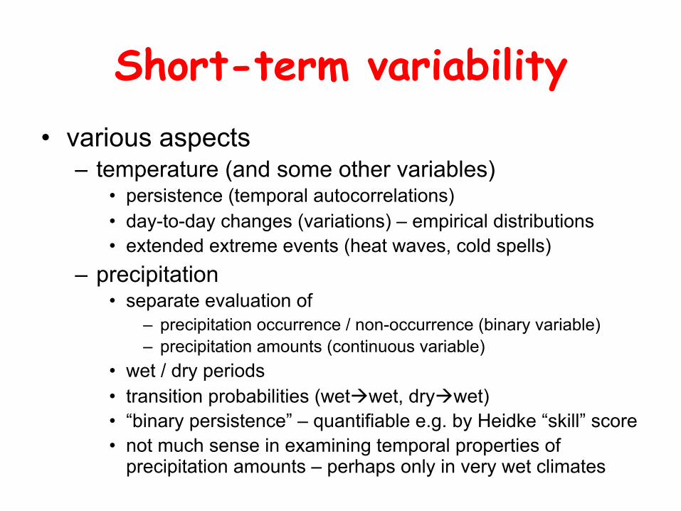
Short-term variability • various aspects
– temperature (and some other variables) • persistence (temporal autocorrelations) • day-to-day changes (variations) – empirical distributions • extended extreme events (heat waves, cold spells)
– precipitation • separate evaluation of
– precipitation occurrence / non-occurrence (binary variable) – precipitation amounts (continuous variable)
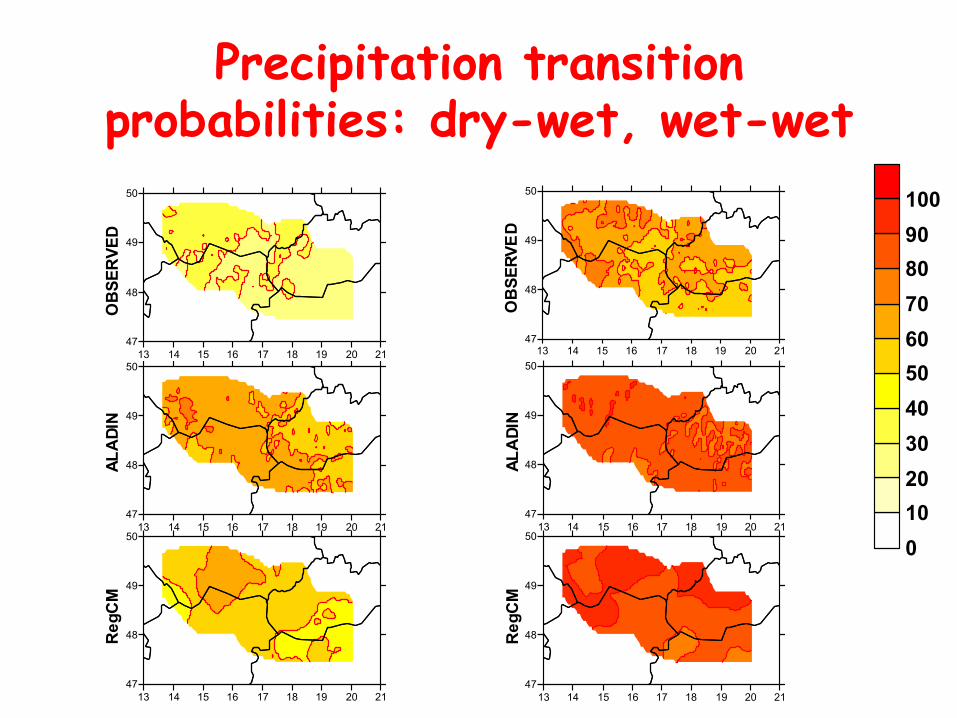
• wet / dry periods • transition probabilities (wetàwet, dryàwet) • “binary persistence” – quantifiable e.g. by Heidke “skill” score • not much sense in examining temporal properties of
precipitation amounts – perhaps only in very wet climates
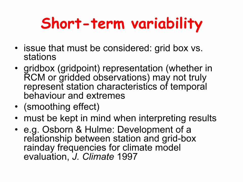
Short-term variability • issue that must be considered: grid box vs.
stations • gridbox (gridpoint) representation (whether in
RCM or gridded observations) may not truly represent station characteristics of temporal behaviour and extremes
• (smoothing effect) • must be kept in mind when interpreting results • e.g. Osborn & Hulme: Development of a
relationship between station and grid-box rainday frequencies for climate model evaluation, J. Climate 1997
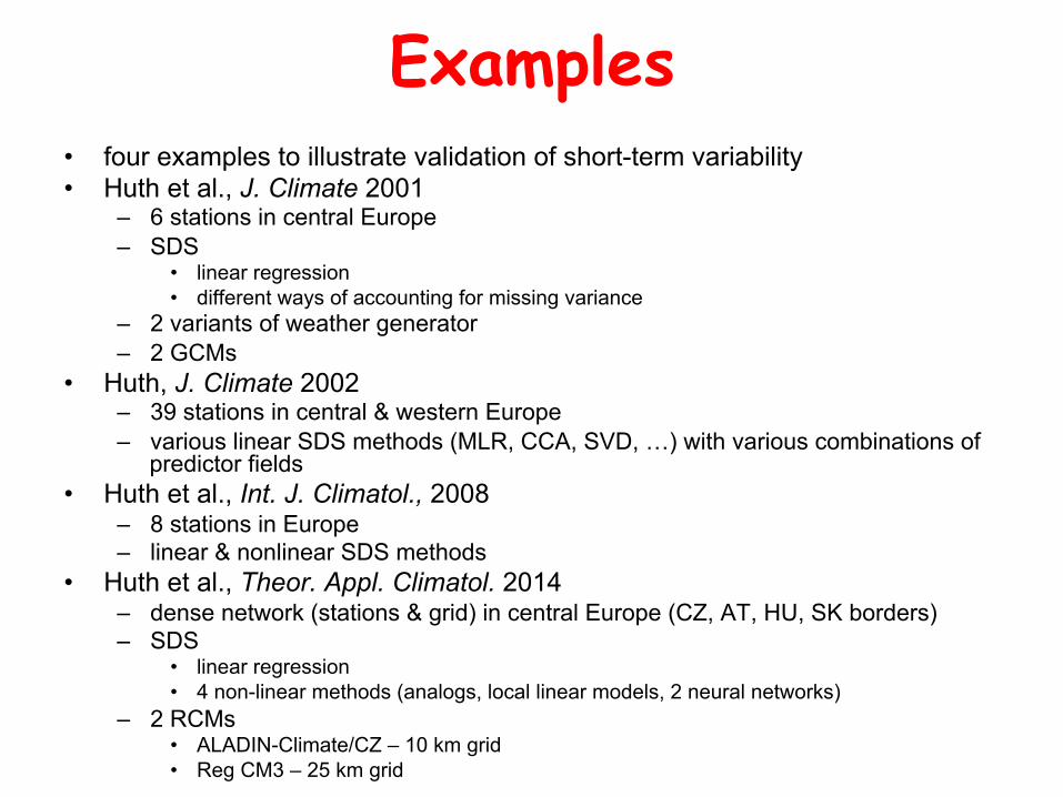
Examples • four examples to illustrate validation of short-term variability • Huth et al., J. Climate 2001
– 6 stations in central Europe – SDS
• linear regression • different ways of accounting for missing variance
– 2 variants of weather generator – 2 GCMs
• Huth, J. Climate 2002 – 39 stations in central & western Europe – various linear SDS methods (MLR, CCA, SVD, …) with various combinations of
predictor fields • Huth et al., Int. J. Climatol., 2008
– 8 stations in Europe – linear & nonlinear SDS methods
• Huth et al., Theor. Appl. Climatol. 2014 – dense network (stations & grid) in central Europe (CZ, AT, HU, SK borders) – SDS
• linear regression • 4 non-linear methods (analogs, local linear models, 2 neural networks)
– 2 RCMs • ALADIN-Climate/CZ – 10 km grid • Reg CM3 – 25 km grid
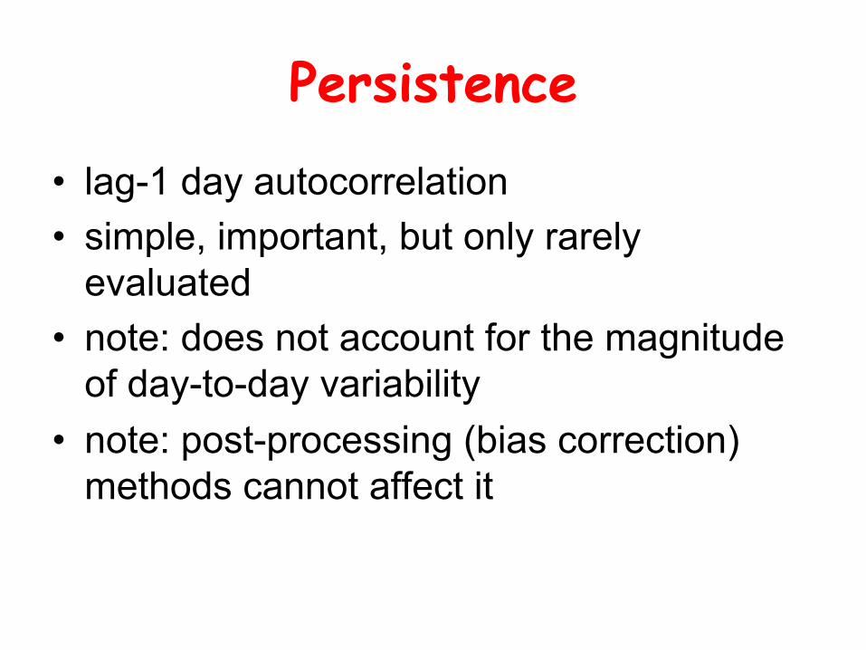
Persistence
• lag-1 day autocorrelation • simple, important, but only rarely
evaluated • note: does not account for the magnitude
of day-to-day variability • note: post-processing (bias correction)
methods cannot affect it
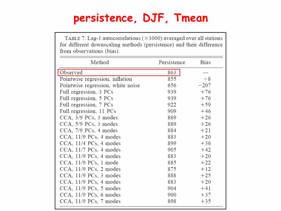
persistence, DJF, Tmean
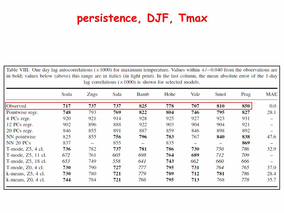
persistence, DJF, Tmax
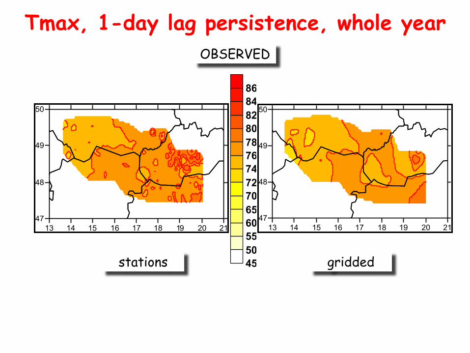
Tmax, 1-day lag persistence, whole year OBSERVED
13 14 15 16 17 18 19 20 2147
48
49
50
4550556065707274767880828486
13 14 15 16 17 18 19 20 2147
48
49
50
13 14 15 16 17 18 19 20 2147
48
49
50
gridded stations
4550556065707274767880828486
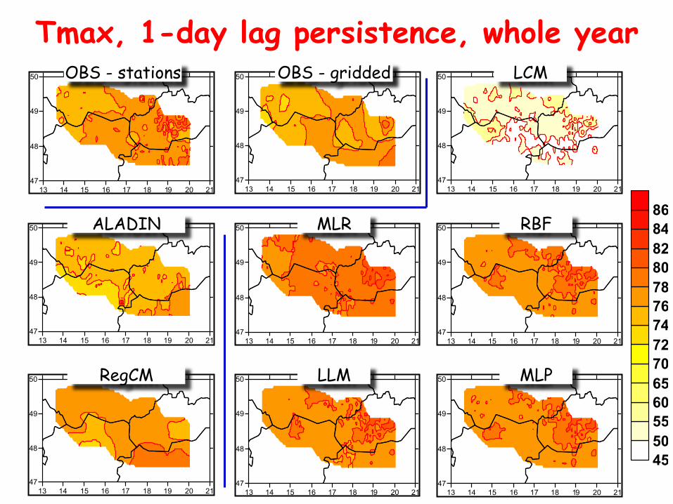
Tmax, 1-day lag persistence, whole year
13 14 15 16 17 18 19 20 2147
48
49
50
13 14 15 16 17 18 19 20 2147
48
49
50
13 14 15 16 17 18 19 20 2147
48
49
50
13 14 15 16 17 18 19 20 2147
48
49
50
13 14 15 16 17 18 19 20 2147
48
49
50
13 14 15 16 17 18 19 20 2147
48
49
50
13 14 15 16 17 18 19 20 2147
48
49
50
13 14 15 16 17 18 19 20 2147
48
49
50
13 14 15 16 17 18 19 20 2147
48
49
50OBS - stations OBS - gridded
ALADIN
RegCM
MLR
LLM
LCM
RBF
MLP
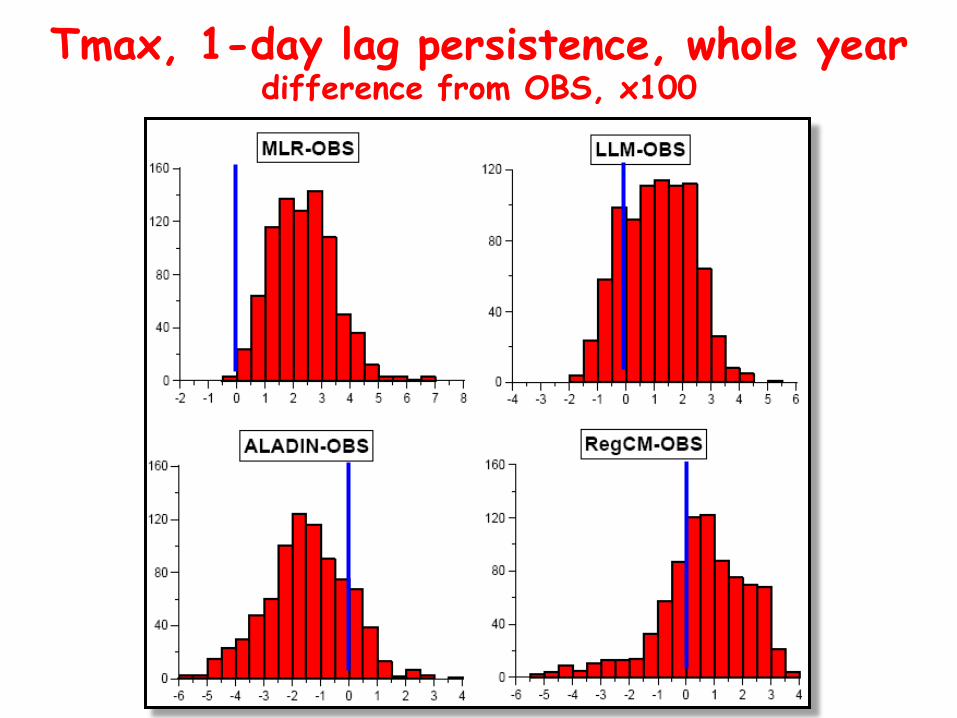
Tmax, 1-day lag persistence, whole year difference from OBS, x100
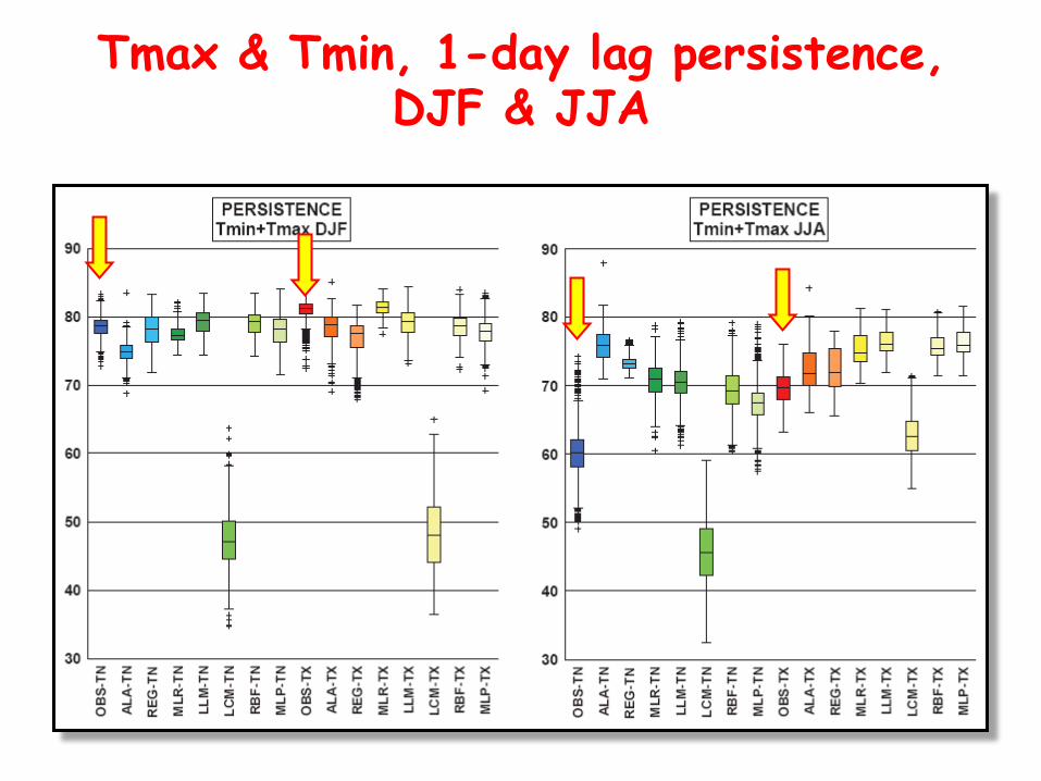
Tmax & Tmin, 1-day lag persistence, DJF & JJA
Day-to-day changes • different aspect of short-term variability • time series with identical persistence may have
very different distributions of day-to-day changes • characteristics of statistical distribution
(histogram) of day-to-day changes are evaluated, namely – standard deviation – skewness (asymmetry)
• reflects the ability of models to include (and correctly simulate) various physical processes (radiation, advection, …)
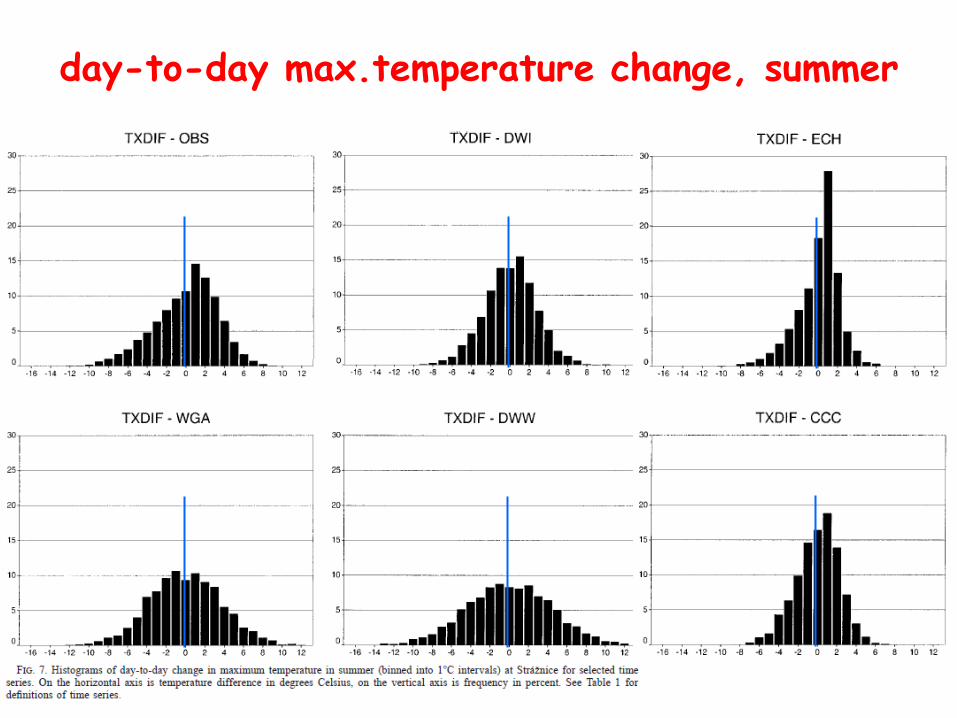
day-to-day max.temperature change, summer
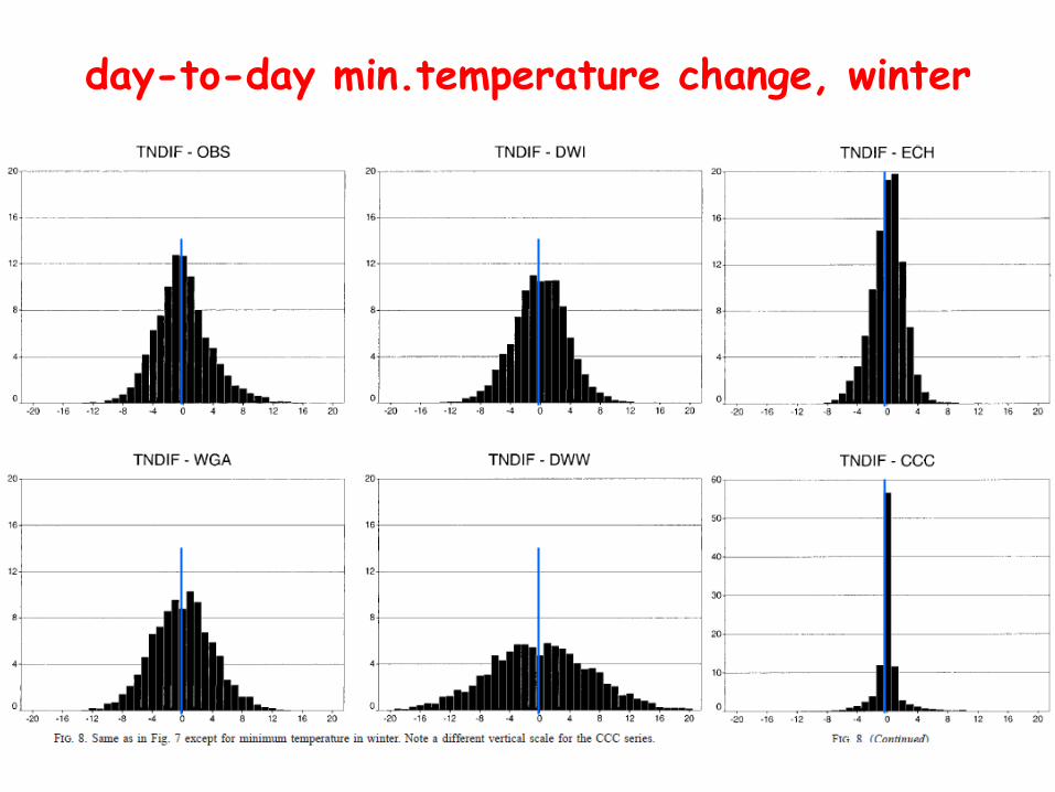
day-to-day min.temperature change, winter
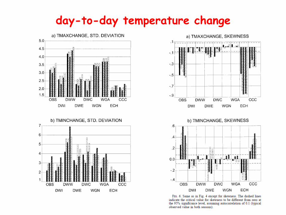
day-to-day temperature change
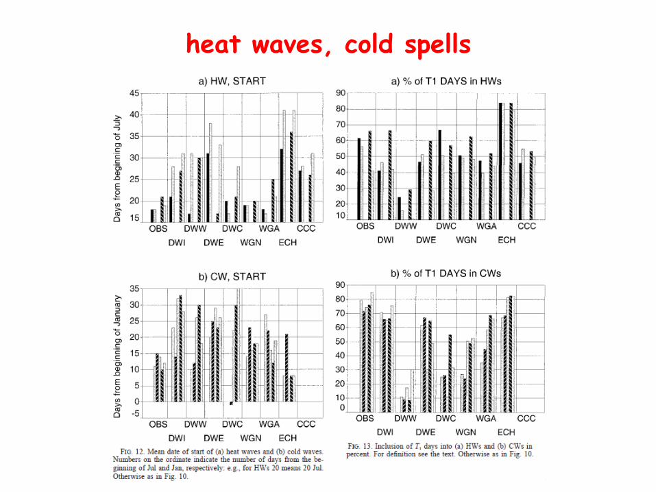
Extended extreme events • important characteristics of extreme weather • potentially big difference if extremes occur individually or in
sequences • examples
– heat waves – cold spells
• typical definition – periods of a certain minimum duration with temperature exceeding a threshold (absolute or percentile-based)
• integral characteristic – integrates different aspects o temperature (extremes, persistence, annual cycle, …)
• possible characteristics to validate – frequency – duration – percentage of extreme days included in extended events (reflects
mainly persistence) – intensity (highest temperature or highest temperature exceedance over
threshold during the event) – date of occurrence (reflects the ability to simulate annual cycle)
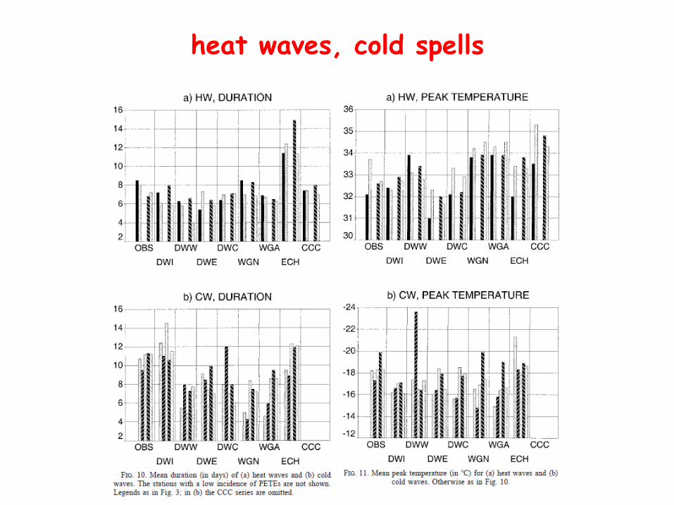
heat waves, cold spells
heat waves, cold spells
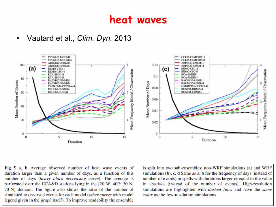
heat waves • Vautard et al., Clim. Dyn. 2013
13 14 15 16 17 18 19 20 2147
48
49
50
0102030405060708090100
Precipitation transition probabilities: dry-wet, wet-wet
13 14 15 16 17 18 19 20 2147
48
49
50
OBSERVED
ALADIN
RegCM
13 14 15 16 17 18 19 20 2147
48
49
50
13 14 15 16 17 18 19 20 2147
48
49
50
13 14 15 16 17 18 19 20 2147
48
49
50
OBSERVED
ALADIN
RegCM
13 14 15 16 17 18 19 20 2147
48
49
50
13 14 15 16 17 18 19 20 2147
48
49
50
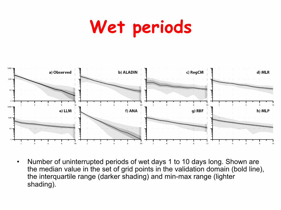
Wet periods
• Number of uninterrupted periods of wet days 1 to 10 days long. Shown are the median value in the set of grid points in the validation domain (bold line), the interquartile range (darker shading) and min-max range (lighter shading).
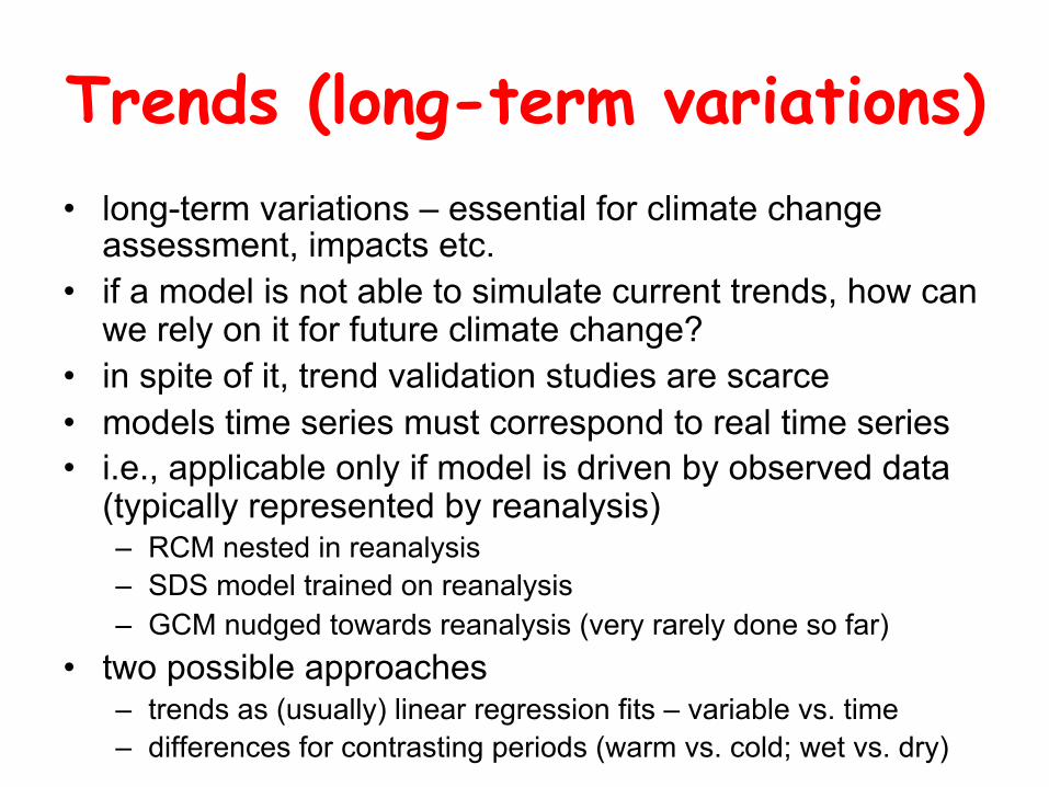
Trends (long-term variations) • long-term variations – essential for climate change
assessment, impacts etc. • if a model is not able to simulate current trends, how can
we rely on it for future climate change? • in spite of it, trend validation studies are scarce • models time series must correspond to real time series • i.e., applicable only if model is driven by observed data
(typically represented by reanalysis) – RCM nested in reanalysis – SDS model trained on reanalysis – GCM nudged towards reanalysis (very rarely done so far)
• two possible approaches – trends as (usually) linear regression fits – variable vs. time – differences for contrasting periods (warm vs. cold; wet vs. dry)
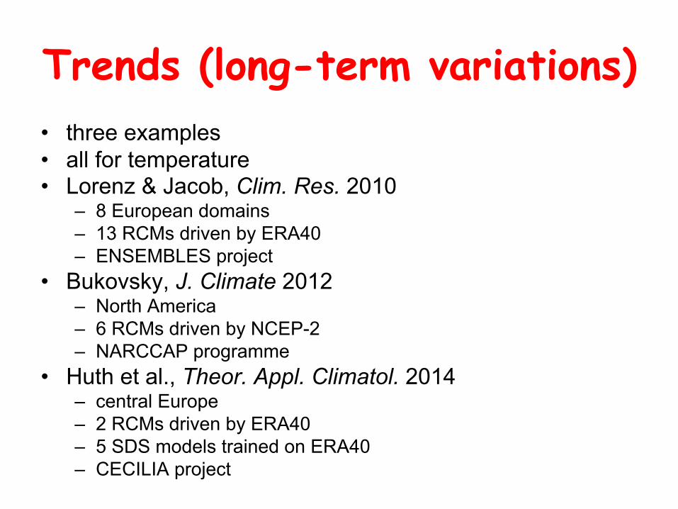
Trends (long-term variations) • three examples • all for temperature • Lorenz & Jacob, Clim. Res. 2010
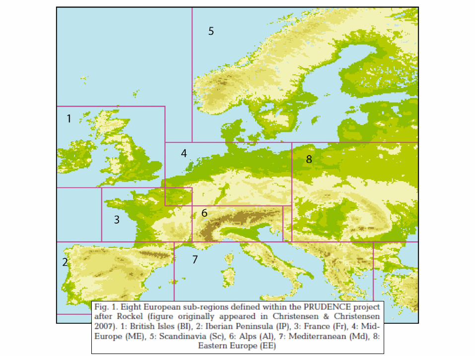
– 8 European domains – 13 RCMs driven by ERA40 – ENSEMBLES project
• Bukovsky, J. Climate 2012 – North America – 6 RCMs driven by NCEP-2 – NARCCAP programme
• Huth et al., Theor. Appl. Climatol. 2014 – central Europe – 2 RCMs driven by ERA40 – 5 SDS models trained on ERA40 – CECILIA project

• trend difference (in °C / decade) from E-OBS • note discrepancies between observed data / reanalyses
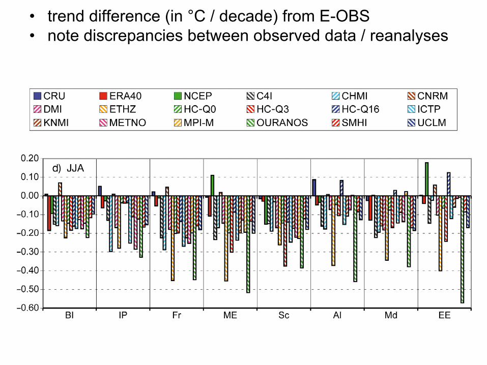
• trend difference (in °C / decade) from E-OBS • note discrepancies between observed data / reanalyses
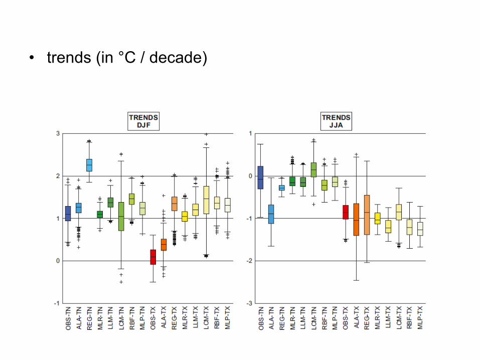
• trends (in °C / decade)
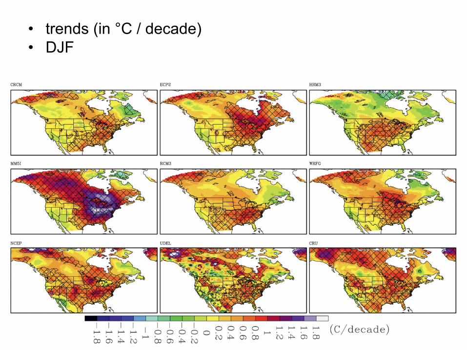
• trends (in °C / decade) • DJF
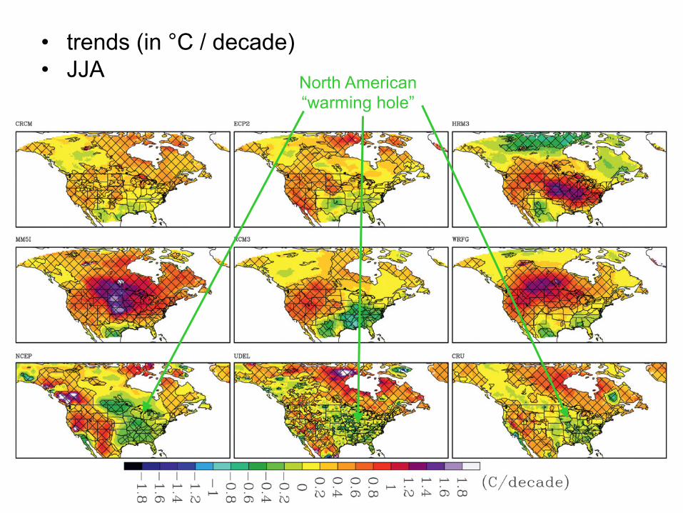
• trends (in °C / decade) • JJA North American
“warming hole”
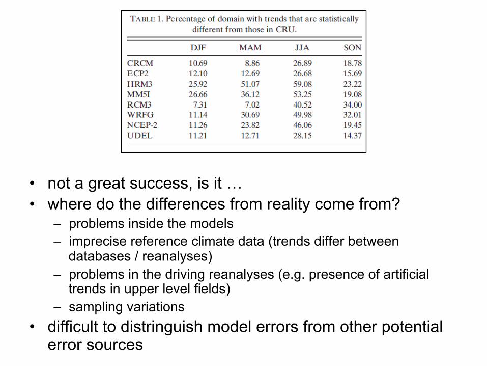
• not a great success, is it … • where do the differences from reality come from?
– problems inside the models – imprecise reference climate data (trends differ between
databases / reanalyses) – problems in the driving reanalyses (e.g. presence of artificial
trends in upper level fields) – sampling variations
• difficult to distringuish model errors from other potential error sources