Temporal Privacy in Wireless Sensor Networks: Theory and Practice

28

Temporal Privacy in Wireless SensorNetworks: Theory and Practice

PANDURANG KAMAT, WENYUAN XU, WADE TRAPPE, and YANYONG ZHANG

Rutgers University

Although the content of sensor messages describing “events of interest” may be encrypted to provideconfidentiality, the context surrounding these events may also be sensitive and therefore shouldbe protected from eavesdroppers. An adversary armed with knowledge of the network deployment,routing algorithms, and the base-station (data sink) location can infer the temporal patterns ofinteresting events by merely monitoring the arrival of packets at the sink, thereby allowing theadversary to remotely track the spatio-temporal evolution of a sensed event. In this paper weintroduce the problem of temporal privacy for delay-tolerant sensor networks, and propose adaptivebuffering at intermediate nodes on the source-sink routing path to obfuscate temporal informationfrom the adversary. We first present the effect of buffering on temporal privacy using an information-theoretic formulation, and then examine the effect that delaying packets has on buffer occupancy.We observe that temporal privacy and efficient buffer utilization are contrary objectives, and thenpresent an adaptive buffering strategy that effectively manages these tradeoffs. Finally, we evaluateour privacy enhancement strategies using simulations, where privacy is quantified in terms of theadversary’s mean square error.

Categories and Subject Descriptors: D.4.6 [Operating Systems]: Security and Protection

General Terms: Security, Algorithms, Design, Measurement, Performance, Theory

Additional Key Words and Phrases: Sensor networks, privacy, security, temporal privacy

ACM Reference Format:

Kamat, P., Xu, W., Trappe, W., and Zhang, Y. 2009. Temporal privacy in wireless sensor net-works: Theory and practice. ACM Trans. Sens. Netw. 5, 4, Article 28 (November 2009), 24 pages.DOI = 10.1145/1614379.1614380 http://doi.acm.org/10.1145/1614379.1614380.

1. INTRODUCTION

Sensor networks are being deployed to monitor a vast array of phenomena.The information surrounding these measurements can have varying levels ofimportance, and for this reason conventional security services, such as encryp-tion and authentication, have been migrated to the sensor domain [Perrig et al.2002; Bohge and Trappe 2003; Karlof and Wagner 2003; Zhu et al. 2003; Chan

Authors’ address: Wireless Information Network Laboratory (WINLAB), Rutgers University, 671Route 1 South, North Brunswick, NJ 08902; email: [email protected] to make digital or hard copies of part or all of this work for personal or classroom useis granted without fee provided that copies are not made or distributed for profit or commercialadvantage and that copies show this notice on the first page or initial screen of a display alongwith the full citation. Copyrights for components of this work owned by others than ACM must behonored. Abstracting with credit is permitted. To copy otherwise, to republish, to post on servers,to redistribute to lists, or to use any component of this work in other works requires prior specificpermission and/or a fee. Permissions may be requested from Publications Dept., ACM, Inc., 2 PennPlaza, Suite 701, New York, NY 10121-0701 USA, fax +1 (212) 869-0481, or [email protected]© 2009 ACM 1550-4859/2009/11-ART28 $10.00DOI 10.1145/1614379.1614380 http://doi.acm.org/10.1145/1614379.1614380

ACM Transactions on Sensor Networks, Vol. 5, No. 4, Article 28, Publication date: November 2009.

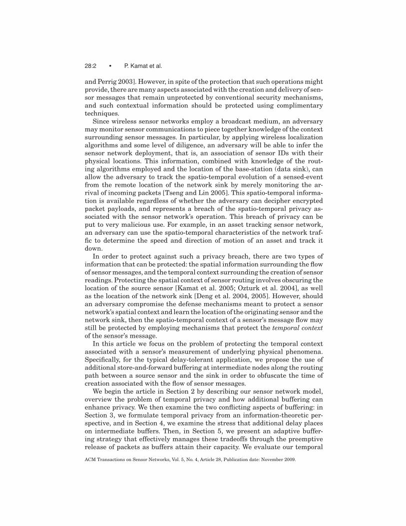
28:2 • P. Kamat et al.

and Perrig 2003]. However, in spite of the protection that such operations mightprovide, there are many aspects associated with the creation and delivery of sen-sor messages that remain unprotected by conventional security mechanisms,and such contextual information should be protected using complimentarytechniques.

Since wireless sensor networks employ a broadcast medium, an adversarymay monitor sensor communications to piece together knowledge of the contextsurrounding sensor messages. In particular, by applying wireless localizationalgorithms and some level of diligence, an adversary will be able to infer thesensor network deployment, that is, an association of sensor IDs with theirphysical locations. This information, combined with knowledge of the rout-ing algorithms employed and the location of the base-station (data sink), canallow the adversary to track the spatio-temporal evolution of a sensed-eventfrom the remote location of the network sink by merely monitoring the ar-rival of incoming packets [Tseng and Lin 2005]. This spatio-temporal informa-tion is available regardless of whether the adversary can decipher encryptedpacket payloads, and represents a breach of the spatio-temporal privacy as-sociated with the sensor network’s operation. This breach of privacy can beput to very malicious use. For example, in an asset tracking sensor network,an adversary can use the spatio-temporal characteristics of the network traf-fic to determine the speed and direction of motion of an asset and track itdown.

In order to protect against such a privacy breach, there are two types ofinformation that can be protected: the spatial information surrounding the flowof sensor messages, and the temporal context surrounding the creation of sensorreadings. Protecting the spatial context of sensor routing involves obscuring thelocation of the source sensor [Kamat et al. 2005; Ozturk et al. 2004], as wellas the location of the network sink [Deng et al. 2004, 2005]. However, shouldan adversary compromise the defense mechanisms meant to protect a sensornetwork’s spatial context and learn the location of the originating sensor and thenetwork sink, then the spatio-temporal context of a sensor’s message flow maystill be protected by employing mechanisms that protect the temporal contextof the sensor’s message.

In this article we focus on the problem of protecting the temporal contextassociated with a sensor’s measurement of underlying physical phenomena.Specifically, for the typical delay-tolerant application, we propose the use ofadditional store-and-forward buffering at intermediate nodes along the routingpath between a source sensor and the sink in order to obfuscate the time ofcreation associated with the flow of sensor messages.

We begin the article in Section 2 by describing our sensor network model,overview the problem of temporal privacy and how additional buffering canenhance privacy. We then examine the two conflicting aspects of buffering: inSection 3, we formulate temporal privacy from an information-theoretic per-spective, and in Section 4, we examine the stress that additional delay placeson intermediate buffers. Then, in Section 5, we present an adaptive buffer-ing strategy that effectively manages these tradeoffs through the preemptiverelease of packets as buffers attain their capacity. We evaluate our temporal


Temporal Privacy in Wireless Sensor Networks • 28:3

privacy solutions in Section 6 through simulations involving a large-scale net-work, where the adversary’s mean square error is used to quantify the temporalprivacy. Finally, we present related work in Section 7, and conclude the articlein Section 8.

2. OVERVIEW OF TEMPORAL PRIVACY IN SENSOR NETWORKS

We start our overview by describing a couple of scenarios that illustrate the is-sues associated with temporal privacy. To begin, consider a sensor network thathas been deployed to monitor an animal habitat [Kamat et al. 2005; Szewczyket al. 2004]. In this scenario, animals (“assets”) move through the environment,their presence is sensed by the sensor network and reported to the networksink. The fact that the network produces data and sends it to the sink providesan indication that the animal was present at the source at a specific time. Ifthe adversary is able to associate the origin time of the packet with a sensor’slocation, then the adversary will be able to track the animal’s behavior—a dan-gerous prospect if the animal is endangered and the adversary is a hunter! Thissame scenario can be easily translated to a tactical environment, where the sen-sor network monitors events in support of military networked operations. Inasset tracking, if we add temporal ambiguity to the time that the packets arecreated then, as the asset moves, this would introduce spatial ambiguity andmake it harder for the adversary to track the asset.

The situations where temporal privacy is important are not always associ-ated with protecting spatio-temporal context, but instead there are scenarioswhere we are solely interested in masking the time at which an event occurred.For example, sensor networks may be deployed to monitor inventory in a ware-house. In this scenario, a sensor would create audit logs associated with theremoval/relocation of items (bearing RFID tags) within the warehouse androute these audit messages to the network sink. Here, an adversary locatednear the sink (perhaps outside the warehouse) could observe packets arrivingand use this information to infer the stock levels or the volume of transactionsgoing through a warehouse at a specific time. Such information could be of greatbenefit to a rival corporation that is interested in knowing its competitor’s salesand inventory profile. Here, if we add temporal ambiguity to the delivery ofthe audit messages, then the warehouse would still be able to verify its inven-tory against purchase orders, but the competitor would have outdated informa-tion about the inventory activity.

For both scenarios, temporal privacy amounts to preventing an adversaryfrom inferring the time of creation associated with one or more sensor packetsarriving at the network sink. In order to protect the temporal context of thepacket’s creation, it is possible to introduce additional, random delay to thedelivery of packets in order to mask a sensor reading’s time of creation. However,although delaying packets might increase temporal privacy, this strategy alsonecessitates the use of buffering within the network and places new stress onthe internal store-and-forward network buffers.

We may define a generic model for both the sensor network and the ad-versary that captures the most relevant features of the temporal privacy



problem in this article. The abstract sensor network model that we will useinvolves:

—Delay-Tolerant Application. A sensor application that is delay-tolerant in thesense that observations can be delayed by reasonable amounts of time be-fore arriving at the monitoring application, thereby allowing us to introduceadditional delay in packet delivery.

—Payload Encrypted. The payload contains application-level information, suchas the sensor reading, application sequence number and the time-stamp as-sociated with the sensor reading. In order to guarantee the confidentiality ofthis data, conventional encryption is employed.

—Headers are Cleartext. The headers associated with essential network func-tionality are not encrypted. For example, the routing header associatedwith Woo et al. [2003], and used in the TinyOS 1.1.7 release (described inMultiHop.h) includes the ID of the previous hop, the ID of the origin (used inthe routing layer to differentiate between whether the packet is being gener-ated or forwarded), the routing-layer sequence number (used to avoid loops,not flow-specific and hence cannot help the adversary in estimating time ofcreation), and the hop count.

On the other hand, the assumptions that we have for the adversary are

—Protocol-Aware. By Kerckhoff ’s Principle [Trappe and Washington 2002], weassume the adversary has knowledge of the networking and privacy protocolsbeing employed by the sensor network. In particular, the adversary knowsthe delay distributions being used by each node in the network.

—Able to Eavesdrop. We assume that the adversary is able to eavesdrop on com-munications in order to read packet headers, or control traffic. We emphasizethat the adversary is not able to decipher packet contents by decrypting thepayloads, and hence the adversary must infer packet creation times solelyfrom network knowledge and the time it witnesses a packet.

—Deployment-Aware. We assume that the adversary at the sink and is awareof the identity of all sensor nodes. Since the adversary can monitor communi-cations, we assume that the adversary knows the source identity associatedwith each transmission. Further, since the adversary is aware of the routingprotocols employed and can eavesdrop, the adversary is able to build its ownsource-sink routing tables.

—Nonintrusive. The adversary does not interfere with the proper functioningof the network, otherwise intrusion detection measures might flag the adver-sary’s presence. In particular, the adversary does not inject or modify packets,alter the routing path, or destroy sensor devices.

Taken together, we note that we have separated out issues associated with ob-scuring the location of the source’s origin, and solely focus on temporal privacy.We note, however, that in practice the combination of temporal privacy methodswith location-privacy methods will yield a more complete solution to protectingcontextual privacy in sensor networks.



3. TEMPORAL PRIVACY FORMULATION

We start by first examining the theoretical underpinnings of temporal privacy.Our discussion will start by first setting up the formulation using a simplenetwork of two nodes transmitting a single packet, and then we extend theformulation to more general network scenarios.

3.1 Temporal Privacy: Two-Party Single-Packet Network

We begin by considering a simple network consisting of a source S, a receivernode R, and an adversarial node E that monitors traffic arriving at R. Thegoal of preserving temporal privacy is to make it difficult for the adversaryto infer the time when a specific packet was created. Suppose that the sourcesensor S observes a phenomena and creates a packet at some time X . In orderto obfuscate the time at which this packet was created, S can choose to locallybuffer the packet for a random amount of time Y before transmitting the packet.Disregarding the negligible time it takes for the packet to traverse the wirelessmedium, both R and E will witness that the packet arrives at a time Z = X +Y .The legitimate receiver can decrypt the payload, which contains a timestampfield describing the correct time of creation. The adversary’s objective is to inferthe time of creation X , and since it cannot decipher the payload, it must make aninference based solely upon the observation of Z and (by Kerckhoff ’s Principle)knowledge of the buffering strategy employed at S.

The ability of E to infer X from Z is controlled by two underlying distribu-tions: first is the a priori distribution f X (x), which describes the knowledge theadversary had for the likelihood of the message creation prior to observing Z ;and second, the delay distribution fY ( y), which the source employs to maskX . The amount of information that E can infer about X from observing Z ismeasured by the mutual information:

I (X ; Z ) = h(X ) − h(X |Z ) = h(Z ) − h(Z |X ) (1)

= h(Z ) − h(Y ), (2)

where h(X ) is the differential entropy of X . For certain choices of f X and fY ,we may directly calculate I (X ; Z ). For example, if X ∼ Exp(λ) (i.e., exponentialwith mean 1/λ), and Y ∼ Exp(λ), then Z ∼ Erlang (2, λ), and h(Z ) = −ψ(2) +ln �(2) − ln(λ) + 2, where ψ(w) is the digamma function and �(w) is the gammafunction. For this case, h(Y ) = 1 − ln λ, and hence I (X ; Z ) = 1 − ψ(2) ≈ 1.077.In other words, roughly 1 nat of information about X is learned by observingZ . For more general distributions, the entropy-power inequality [Cover andThomas 1991] gives a lower bound

I (X ; Z ) ≥ 12 ln 2

(22h(X ) + 22h(Y )

)− h(Y ). (3)

In general, however, the distribution for X is fixed and determined by an un-derlying physical phenomena being monitored by the sensor. Since the objectiveof the temporal privacy-enhancing buffering is to hide X , we may formulate thetemporal privacy problem as

minfY ( y)

I (X ; Z ) = h(X + Y ) − h(Y ),



or in other words, choose a delay distribution fY so that the adversary learnsas little as possible about X from Z .1

3.2 Temporal Privacy: Two-Party Multiple-Packet Network

We now extend the formulation of temporal privacy to the more general caseof a source S sending a stream of packets to a receiver R in the presence of anadversary E. In this case, the sender S will create a stream of packets at timesX 1, X 2, . . . , X n, . . . , and will delay their transmissions by Y1, Y2, . . . , Yn, . . . .

The packets will be observed by E at times Z1, Z2, . . . , Zn, . . . . In going tothe more general case of a packet stream, several new issues arise. First, asnoted earlier in Section 2, when we delay multiple packets it will be necessary tobuffer these packets. For now we will hold off on discussing queuing issues untilSection 4. The next issue involves how the packets should be delayed. Thereare many possibilities here. For example, one possibility would have packetsreleased in the same order as their creation, that is, Z1 < Z2 < . . . < Zn,which would correspond to choosing Y j to be at least the wait time needed toflush out all previous packets. Such a strategy does not reflect the fact thatmost sensor monitoring applications do not require that packet ordering ismaintained. Therefore, a more natural delay strategy would involve choosingY j independent of each other and independent of the creation process {X j }.Consequently, there will not be an ordering of (Z1, Z2, . . . , Zn, . . .).

In our sensor network model, however, we assumed that the sensing appli-cation’s sequence number field was contained in the encrypted payload, andconsequently the adversary does not directly observe (Z1, Z2, . . . , Zn, . . .), butinstead observes the sorted process ˜{Z j } = ϒ({Z j }), where ϒ({Z j }) denotesthe permutations needed to achieve a temporal ordering of the elements of theprocess {Z j }, that is, ˜{Z j } = (Z̃1, Z̃2, . . . , Z̃n, . . .) where Z̃1 < Z̃2 < · · · . Theadversary’s task thus becomes inferring the process {X j } from the sorted pro-cess {Z̃ j }. The amount of information gleaned by the adversary after observingZ̃ n = (Z̃1, . . . , Z̃n) is thus I (X n; Z̃ n), and the temporal-privacy objective of thesystem designer is to make I (X n; Z̃ n) small.

Although it is analytically cumbersome to access I (X n; Z̃ n), we may use thedata processing inequality [Cover and Thomas 1991] on X n → Z n → Z̃ n toobtain the relationship 0 ≤ I (X n, Z̃ n) ≤ I (X n, Z n), which allows us to useI (X n, Z n) in a pinching argument to control I (X n, Z̃ n). Expanding I (X n, Z n)as

I (X n, Z n) = h(Z n) − h(Y n) (4)

≤n∑

j=1

(h(Z j ) − h(Y j )

)(5)

=n∑

j=1

I (X j , Z j ), (6)

1The astute reader will note the similarity with the information-theoretic formulation of commu-nication, where the objective is to maximize mutual information.



we may thus bound I (X n, Z n) using the sum of individual mutual informationterms.

As before, the objective of temporal privacy enhancement is to minimizethe information that the adversary gains, and hence to mask {X j }, we shouldminimize I (X n, Z n). Although there are many choices for the delay process {Y j },the general task of finding a nontrivial stochastic process {Y j } that minimizesthe mutual information for a specific temporal process {X j } is challenging andfurther depends on the sensor network design constraints (e.g. buffer storage).In spite of this, however, we may seek to optimize within a specific type ofprocess {Y j }, and from this make some general observations.

As an example of this, let us look at an important and natural example.Suppose that the source sensor creates packets at times {X j } as a Poissonprocess of rate λ, that is, the interarrival times Aj are exponential with mean1/λ, and that the delay process {Y j } corresponds to each Y j being an exponentialdelay with mean 1/μ. One motivation for choosing an exponential distributionfor the delay is the well-known fact that the exponential distribution yieldsmaximal entropy for nonnegative distributions. We note that X j = ∑ j

k=1 Ak

(and hence the X j are j-stage Erlangian random variables with mean j/λ).Using the result of Theorem 3(d) from Anantharam and Verdu [1996], we havethat

I (X j ; Z j ) = I (X j ; X j + Y j )

= ln(

1 + jμλ

)− D

(f X j +Y j ‖ f X j +Y j

)

≤ ln(

1 + jμλ

).

Here, the D( f ‖g ) corresponds to the divergence between two distributions fand g , while X is the mixture of a point mass and exponential distribution withthe same mean as X , as introduced in Anantharam and Verdu [1996]. Sincedivergence is nonnegative and we are only interested in pinching I (X n; Z̃ n), wemay discard this auxiliary term. Using that result, we have that

I (X n, Z n) ≤n∑

j=1

ln(

1 + jμλ

). (7)

Our objective is to make

0 ≤ I (X n; Z̃ n) ≤ I (X n, Z n) ≤n∑

j=1

ln(

1 + jμλ

)

small, and from this we can see that by tuning μ to be small relative to λ (orequivalently, the average delay time 1/μ to be large relative to the averageinterarrival time 1/λ), we can control the amount of information the adversarylearns about the original packet creation times. It is clear that choosing μ toosmall will place a heavy load on the source’s buffer. We will revisit buffer issuesin Section 4 and Section 5.



3.3 Temporal Privacy: Multihop Networks

In the previous subsection, we considered a simple network case consisting oftwo nodes, where the source performs all of the buffering. More general sensornetworks consist of multiple nodes that communicate via multihop routing toa sensor network sink. For such networks, the burden of obfuscating the timesat which a source node creates packets can be shared among other nodes on thepath between the source and the sensor network sink.

To explain, we may consider a generic sensor network consisting of an abun-dant supply of sensor nodes, and focus on an N -hop routing path between thesource and the network sink. By doing so, we are restricting our attention toa line-topology network S → F1 → F2 → · · · → FN−1 → R, where R denotesthe receiving network sink, and F j denotes the j -th intermediate node on theforwarding path.

By introducing multiple nodes, the delay process {Y j } can be decomposedacross multiple nodes as

Y j = Y0 j + Y1 j + · · · + YN−1, j ,

where Ykj denotes the delay introduced at node k for the j -th packet (we useY0 j to denote the delay used by the source node S). Thus, each node k willbuffer each packet j that it receives for a random amount of time Ykj.

This decomposition of the delay process {Y j } into subdelay processes {Ykj } al-lows for great flexibility in achieving both temporal privacy goals and ensuringsuitable buffer utilization in the sensor network. For example, it is well knownthat traffic loads in sensor networks accumulate near network sinks, and itmay be possible to decompose {Y j } so that more delay is introduced when aforwarding node is further from the sink.

4. QUEUING ANALYSIS OF PRIVACY-ENHANCING BUFFERING

Although delaying packets might increase temporal privacy, such a strategyplaces a burden on intermediate buffers. In this section we will examine theunderlying issues of buffer utilization when employing delay to enhance tem-poral privacy.

When using buffering to enhance temporal privacy, each node on the routingpath will receive packets and delay their forwarding by a random amount oftime. As a result, sensor nodes must buffer packets prior to releasing them, andwe may formulate the buffer occupancy using a queuing model. In order to startour discussion, let us again examine the simple two-node case where a sourcenode S generates packets according to an underlying process and the packetsare delayed according to an exponential distribution with average delay 1/μ,prior to being forwarded to the receiver R, as depicted in Figure 1(a). If weassume that the creation process is Poisson with rate λ (if the process is notPoisson, the source may introduce additional delay to shape the traffic), then thebuffering process can be viewed as an M/M/∞ queue where, as new packetsarrive at the buffer, they are assigned to a new “variable-delay server” thatprocesses each packet according to an exponential distribution with mean 1/μ.Following the standard results for M/M/∞ queues, we have that the amount



RS μλ λ

(a)

......S R......μ 1

λ λ λ λ λλμ i μ n

(b)

r/2

i

d1

Sinkφ

r/2

r/2r/2

d2

(c)

μ i

λ iλ iλ 1

i

λ mi

(d)

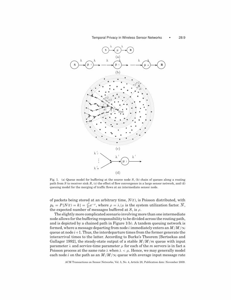
Fig. 1. (a) Queue model for buffering at the source node S, (b) chain of queues along a routingpath from S to receiver sink R, (c) the effect of flow convergence in a large sensor network, and (d)queuing model for the merging of traffic flows at an intermediate sensor node.

of packets being stored at an arbitrary time, N (t), is Poisson distributed, withpk = P{N (t) = k} = ρk

k! e−ρ , where ρ = λ/μ is the system utilization factor. N ,the expected number of messages buffered at S, is ρ.

The slightly more complicated scenario involving more than one intermediatenode allows for the buffering responsibility to be divided across the routing path,and is depicted by a chained path in Figure 1(b). A tandem queuing network isformed, where a message departing from node i immediately enters an M/M/∞queue at node i+1. Thus, the interdeparture times from the former generate theinterarrival times to the latter. According to Burke’s Theorem [Bertsekas andGallager 1992], the steady-state output of a stable M/M/m queue with inputparameter λ and service-time parameter μ for each of the m servers is in fact aPoisson process at the same rate λ when λ < μ. Hence, we may generally modeleach node i on the path as an M/M/∞ queue with average input message rate



λ, but with average service-time 1/μi (to allow each node to follow its own delaydistribution).

So far we have only considered a single routing path in a sensor network,but in practice the network will monitor multiple phenomena simultaneously,and consequently there will be multiple source-sink flows traversing the net-work. As a result, for the most general scenario, the topological structure ofthe network will have an impact on buffer occupancy. For example, nodes thatare closer to network sink typically have higher traffic loads, and thus will beexpected to suffer from a higher buffer occupancy than nodes further from thesink. We now explore this behavior, and the relationship between buffering forprivacy-enhancement and the traffic load placed on intermediate nodes due toflow convergence in the sensor network.

Consider a sensor network deployment as depicted in Figure 1(c), where wehave assumed (without loss of generality) that there is only one sink. Here,multiple sensors generate messages intended for the sink, and each messageis routed in a hop-by-hop manner based on a routing tree (as suggested in thefigure). Message streams merge progressively as they approach the sink. Ifwe assume that the senders in the network generate Poisson flows, then bythe superposition property of Poisson processes, the combined stream arrivingat node i of m independent Poisson processes with rate λi

j is a Poisson pro-cess with rate λi = λi

1 + λi2 + · · · + λi

m. We depict this phenomena for node iin Figure 1(d), where m is the number of “routing” children for node i. Addi-tionally, we let 1/μi be the average buffer delay injected by node i. Then nodei is an M/M/∞ queue, with arrival parameter λi and departure parameterμi, yielding:

—Ni(t), the number of packets in the buffer at node i, is Poisson distributed.

— pik = P{Ni(t) = k} = ρki

k! e−ρi , where ρi = λi/μi.

—The expected number of messages at node i is Ni = ρi.

As expected, if we choose our delay strategy at node i such that μi is muchsmaller than λi (as is desirable for enhanced temporal privacy), then the ex-pected buffer occupancy Ni will be large. Thus, temporal privacy and bufferutilization are conflicting system objectives.

We now evaluate the impact of the depth of node i in the routing tree (thenumber of hops from the node i to the sink). For the sake of calculations, we shallassume that the density η of the sensor deployment is sufficient that a commu-nicating sensor node will always find a path to the network sink. Additionally,let us denote the average geographical distance between parents and childrenin the routing tree by r. Then, to quantify the effect of flow convergence on thelocal traffic rate in the sensor network, let us assume that an outer annulus O1

of distance d1, angular spread ϕ and width r creates a total traffic of rate λO1

packets/second, as depicted in Figure 1(c). Hence, in a spatial ensemble sense,each node carries an average traffic rate of λO1 = λO1/(ϕrd1η). This traffic flowstoward the sink, and if we examine an annulus at distance d2 < d1 with widthr and spread ϕ, the area of this annulus is ϕrd2, and there will be an average ofϕrd2η sensors in O2 carrying a total rate of λO1 . Hence, on average, each sensor



in this inner annulus will carry traffic of rate λO2 = λO1/(ϕrd2η). Comparingthe average traffic load λO2 that a single sensor in an inner annulus O2 carrieswith the average traffic load λO1 of a single sensor in annulus O1, yields

λO2

λO1

= d1

d2, (8)

and hence traffic load increases in inverse relationship to the distance a nodeis from the sink.

The last issue that we need to consider is the amount of storage availablefor buffering at each sensor. As sensors are resource-constrained devices, it ismore accurate to replace the M/M/∞ queues with M/M/k/k queues, wherememory limitations imply that there are at most k servers/buffer slots, andeach buffer slot is able to handle 1 message. If an arriving packet finds all kbuffer slots full, then either the packet is dropped or, as we shall describe inSection 5, a preemption strategy can be employed. For now, we just considerpacket dropping. We note that packet dropping at a single node causes theoutgoing process to lose its Poisson characteristics. However, we further notethat by Kleinrock’s Independence approximation (the merging of several packetstreams has an affect akin to restoring the independence of interarrival times)[Bertsekas and Gallager 1992], we may continue to approximate the incomingprocess at node i as a Poisson process with aggregate rate λi. Hence, in thesame way as we used a tree of M/M/∞ queues to model the network earlier,we can instead model the network as a tree of M/M/k/k queues.

The M/M/k/k formulation provides us with a means to adaptively designthe buffering strategy at each node. If we suppose that the aggregate trafficlevels arriving at a sensor node is λ, then the packet drop rate (the probabilitythat a new packet finds all k buffer slots full) is given by the well-known ErlangLoss formula for M/M/k/k queues:

E(ρ , k) = ρk

k!p0 =

ρk

k!∑ki=0

ρi

i!

, (9)

where ρ = λ/μ. For an incoming traffic rate λ, we may use the Erlang Lossformula to appropriately select μ so as to have a target packet drop rate α whenusing buffering to enhance privacy. This observation is powerful as it allows usadjust the buffer delay parameter μ at different locations in the sensor network,while maintaining a desired buffer performance. In particular, the expressionfor E(ρ , k) implies that, as we approach the sink and the traffic rate λ increases,we must decrease the average delay time 1/μ in order to maintain E(ρ , k) at atarget packet drop rate α.

5. RCAD: RATE-CONTROLLED ADAPTIVE DELAYING

A consequence of the results of the previous section is that nodes close to the sinkwill have high buffer demands and their buffers may be full when new packetsarrive. In practice, we need to adjust the delay distribution as a function of theincoming traffic rate and the available buffer space.



In order to accomplish this adjustment, we propose RCAD, a Rate-ControlledAdaptive Delaying mechanism, to achieve privacy and desirable performancesimultaneously. The main idea behind RCAD is buffer preemption—if the bufferis full, a node should select an appropriate buffered packet, called the victimpacket, and transmit it immediately rather than drop packets. Consequently,preemption automatically adjusts the effective μ based on buffer state. In thispaper, we have proposed the following buffer preemption policies:

—Longest Delayed First (LDF). In this policy, the victim packet is the packetthat has stayed in the buffer the longest. By doing so, we can ensure thateach packet is buffered for at least a short duration. The implementation ofthis policy requires that each node record the arrival time of every packet.

—Longest Remaining Delay First (LRDF). In this policy, the victim packet is thepacket that has the longest remaining delay time. Preempting such packetscan lessen the buffer load more than any other policy because such pack-ets would have resided in the buffer the longest. The implementation of thisscheme is straightforward because each node already keeps track of the re-maining buffer time for every packet.

—Shortest Delay Time First (SDTF). In this policy, the victim packet is theone with the shortest delay time. By lessening an already short delay time,we expect that the overall performance will remain roughly the same. Theimplementation of this policy requires each node record the delay of everypacket.

—Shortest Remaining Delay First (SRDF). In this policy, the victim packet is thepacket that has the shortest remaining delay time. In this way, the resultingdelay times for that node are the closest to the original distribution. As inthe case of the LRDF policy, the implementation is straightforward.

6. EVALUATING RCAD USING SIMULATIONS

In this study, we have developed a detailed event-driven simulator to studythe performance of RCAD. The simulations modeled realistic network/trafficsettings, and measured important performance and privacy metrics.

6.1 Performance Metrics and Adversary Models

In our simulated sensor network, we have multiple source nodes that createpackets, and intermediate nodes that follow RCAD schemes for buffering pack-ets prior to forwarding them. As an important player of the game, the adversarystays at the sink, observes packet arrivals, and estimates the creation times ofthese packets.

In this study, we assume a powerful adversary that can acquire the fol-lowing parameters for each flow: (1) the hop count of that flow, (2) the delaydistributions for nodes along the flow, and (3) the traffic arrival process of theflow, for example, the arrival rate, the arrival distribution, etc. For an observedpacket arrival time z, a baseline adversary estimates the creation time of thispacket as x ′ = z − y , where y is the average delay of the flow, which theadversary can calculate from its knowledge of the delay distributions. In the



simulations, we use the square error to quantify the estimation error, that is,(x ′ − x)2 where x is the true creation time. Similarly, for a series of packet ar-rivals from the same flow z1, z2, . . . , zm, a baseline adversary estimates theircreation times as x ′

1, x ′2, . . . , x ′

m, and x ′i = zi − y . The total estimation error

for m packets is then calculated as the mean square error,∑

(x ′i − xi)2/m.

We note that there is a direct relationship between mutual information andmean square error [Guo et al. 2005], and hence the scheme that has a higherestimation error consequently better preserves the temporal privacy of thesource.

Since RCAD schemes dynamically adapt the delay processes by adoptingbuffer preemption strategies, it is inadequate for the adversary to estimate theactual delay times using the original delay distributions before preemption. Asa result, we also enhance the baseline adversary to let the adversary adapt hisestimation of the delays. We call such an adversary as an adaptive adversary.

In order to understand our adaptive adversary model, let us first look ata simple example. Let us assume there is only one node with one buffer slotbetween the source and sink. Further, assume that the packet arrival followsa Poisson process with rate λ, and the buffer generates a random delay timethat follows an exponential distribution with mean 1/μ. If the buffer at theintermediate node is full when a new packet arrives, the currently bufferedpacket will be transmitted. In this example, if the traffic rate is low, say λ < μ,then the packet delay time will be 1/μ. However, as the traffic increases, theaverage delay time will become 1/λ due to buffer preemptions. Following thisexample, our adaptive adversary should adopt a similar estimation strategy:at low traffic rates, he estimates the overall average delay y by h/μ, while athigher traffic rates, he estimates the overall average delay y as a function of thebuffer space and the incoming rate, that is, hk/λ, where h is the flow hop count,k is the number of buffer slots at each node, and λ is the traffic rate of thatflow. Given an aggregated traffic rate λtot from n sources converging at leastone-hop prior to the sink, the adversary can compute the probability of bufferoverflow via the Erlang Loss formula in Equation (9). He then can comparethis against a chosen threshold and if the probability is less than the threshold,he will assume the average delay introduced by each hop is 1/μ. However, ifthe probability is higher than the threshold, the average delay at each node iscalculated to be nk/λtot .

Additionally, we note that it is desirable to achieve privacy while maintainingtolerable end-to-end delivery latency for each packet. Hence, in our studies, fora network performance metric we use the average end-to-end delivery latencyfor packets coming from a particular flow versus the underlying traffic rate andthe RCAD strategies employed.

6.2 Simulation Setup

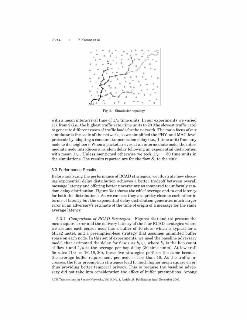
The topology that we considered in our simulations is illustrated in Figure 2.Here, nodes S1, S2, S3, and S4 are source nodes and create packets that aredestined for the sink. Thus, we had four flows, and these flows had hop counts15, 22, 9, and 11 respectively. Each source generated a total of 1000 packets



Sink

S4

S1

S2

S3

Fig. 2. Simulation topology.

with a mean interarrival time of 1/λ time units. In our experiments we varied1/λ from 2 (i.e., the highest traffic rate) time units to 20 (the slowest traffic rate)to generate different cases of traffic loads for the network. The main focus of oursimulator is the scale of the network, so we simplified the PHY- and MAC-levelprotocols by adopting a constant transmission delay (i.e., 1 time unit) from anynode to its neighbors. When a packet arrives at an intermediate node, the inter-mediate node introduces a random delay following an exponential distributionwith mean 1/μ. Unless mentioned otherwise we took 1/μ = 30 time units inthe simulations. The results reported are for the flow S1 to the sink.

6.3 Performance Results

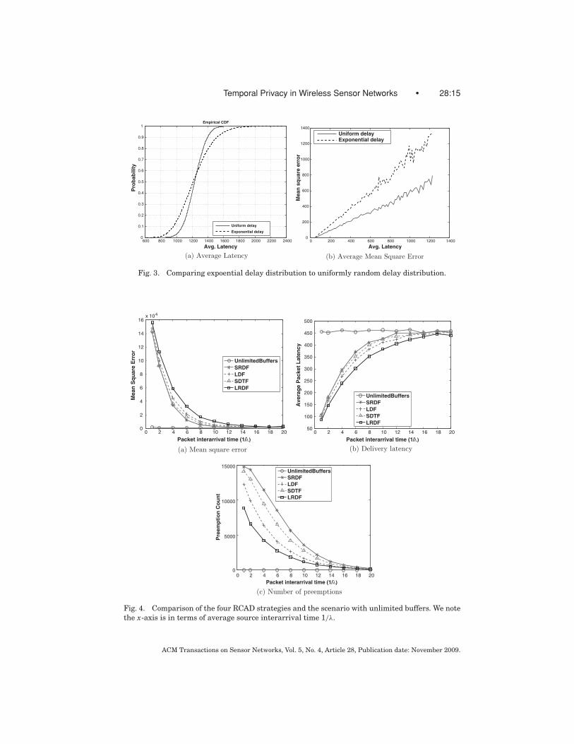
Before analyzing the performance of RCAD strategies, we illustrate how choos-ing exponential delay distribution achieves a better tradeoff between overallmessage latency and offering better uncertainty as compared to uniformly ran-dom delay distribution. Figure 3(a) shows the cdf of average end-to-end latencyfor both the distributions. As we can see they are pretty close to each other interms of latency but the exponential delay distribution generates much largererror in an adversary’s estimate of the time of origin of a message for the sameaverage latency.

6.3.1 Comparison of RCAD Strategies. Figures 4(a) and (b) present themean square error and the delivery latency of the four RCAD strategies wherewe assume each sensor node has a buffer of 10 slots (which is typical for aMica2 mote), and a preemption-less strategy that assumes unlimited bufferspace on each node. In this set of experiments, we used the baseline adversarymodel that estimated the delay for flow i as hi/μ, where hi is the hop countof flow i and 1/μ is the average per hop delay (30 time units). At low traf-fic rates (1/λ = 16, 18, 20), these five strategies perform the same becausethe average buffer requirement per node is less than 10. As the traffic in-creases, the four preemption strategies lead to much higher mean square error,thus providing better temporal privacy. This is because the baseline adver-sary did not take into consideration the effect of buffer preemptions. Among



600 800 1000 1200 1400 1600 1800 2000 2200 24000

0.1

0.2

0.3

0.4

0.5

0.6

0.7

0.8

0.9

1

Avg. Latency

Pro

ba

bil

ity

Empirical CDF

Uniform delay

Exponential delay

0 200 400 600 800 1000 1200 14000

200

400

600

800

1000

1200

1400

Avg. Latency

Me

an

sq

ua

re e

rro

r

Uniform delayExponential delay

(a) Average Latency (b) Average Mean Square Error

Fig. 3. Comparing expoential delay distribution to uniformly random delay distribution.

0 2 4 6 8 10 12 14 16 18 200

2

4

6

8

10

12

14

16x 104

Packet interarrival time (1/λ)

Me

an

Sq

ua

re E

rro

r

UnlimitedBuffers

SRDF

LDF

SDTF

LRDF

0 2 4 6 8 10 12 14 16 18 2050

100

150

200

250

300

350

400

450

500


Avera

ge P

acket

Late

ncy

UnlimitedBuffers

SRDF

LDF

SDTF

LRDF

(a) Mean square error

0 2 4 6 8 10 12 14 16 18 200

5000

10000

15000


Pre

em

pti

on

Co

un

t

UnlimitedBuffers

SRDF

LDF

SDTF

LRDF

(c) Number of preemptions

(b) Delivery latency

Fig. 4. Comparison of the four RCAD strategies and the scenario with unlimited buffers. We notethe x-axis is in terms of average source interarrival time 1/λ.



the four RCAD strategies, we observed that LRDF policy consistently performsthe best in terms of privacy, followed by LDF and SDTF, while SRDF was theworst.

In order to understand the difference between these four strategies, let uslook at more detailed statistics. Figure 4(c) presents the number of preemp-tions that occurred during the experiments. We observe the opposite orderhere: the strategy that provides the most privacy incurred the least numberof preemptions. This may appear counterintuitive at first glance, but can besimply explained: the strategy that leads to more preemptions tends to alterthe original delay distribution less, and thus confuses the adversary less. Forexample, LRDF selects the packet that has the longest remaining delay timeas the victim packet. Preempting these packets will have two effects: (1) it willalter the original delay distribution more, and (2) it will reduce the number ofpreemptions.

Moving our attention to delivery latency, we observed that the preemption-less strategy with unlimited buffers incurred much longer latencies at highertraffic rates. Among the four preemption strategies, LRDF has the shortestlatency because it tends to reduce the delay times in the buffer the most.

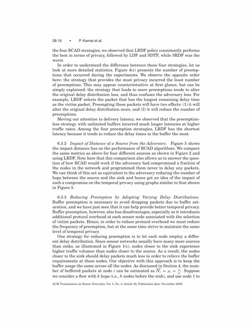
6.3.2 Impact of Distance of a Source from the Adversary. Figure 5 showsthe impact distance has on the performance of RCAD algorithms. We comparethe same metrics as above for four different sources as shown in Figure 2 andusing LRDF. Note here that this comparison also allows us to answer the ques-tion of how RCAD would work if the adversary had compromised a fraction ofthe nodes in the network and programmed them never to delay any packets.We can think of this act as equivalent to the adversary reducing the number ofhops between the source and the sink and hence get an idea of the impact ofsuch a compromise on the temporal privacy using graphs similar to that shownin Figure 5.

6.3.3 Reducing Preemption by Adopting Varying Delay Distributions.Buffer preemption is necessary to avoid dropping packets due to buffer sat-uration, and we have just seen that it can help provide better temporal privacy.Buffer preemption, however, also has disadvantages, especially as it introducesadditional protocol overhead at each sensor node associated with the selectionof victim packets. Hence, in order to reduce protocol overhead we must reducethe frequency of preemption, but at the same time strive to maintain the samelevel of temporal privacy.

One strategy for reducing preemption is to let each node employ a differ-ent delay distribution. Since sensor networks usually have many more sourcesthan sinks, as illustrated in Figure 1(c), nodes closer to the sink experiencehigher traffic volumes than nodes closer to the source. As a result, the nodescloser to the sink should delay packets much less in order to relieve the bufferrequirements at these nodes. Our objective with this approach is to keep thebuffer usage the same across all the nodes. As discussed in Section 4, the num-ber of buffered packets at node i can be estimated as Ni = ρi = λi

μi. Suppose

we consider a flow with h hops (i.e., h nodes before the sink), and use node 1 to



0 2 4 6 8 10 12 14 16 18 200

0.5

1

1.5

2

2.5

3x 105


Mean

Sq

uare

Err

or

One

Two

Three

Four

0 2 4 6 8 10 12 14 16 18 200

100

200

300

400

500

600

700


Avera

ge P

acket

Late

ncy

One

Two

Three

Four


0 2 4 6 8 10 12 14 16 18 200

2000

4000

6000

8000

10000

12000


Pre

em

pti

on

Co

un

t

One

Two

Three

Four

(c) Number of preemptions


Fig. 5. Comparison of the LRDF algorithm for four different source-sink distances. We note thex-axis is in terms of average source interarrival time 1/λ.

denote the last node before the sink and node h to denote the source node. Tokeep Ni constant across all nodes while having a target overall average delayof D, we choose the average delay time 1/μi for node i as β/hi, where β is thecoefficient and hi is the hop count between node i and the sink. Thus, we have∑h

i=1β

hi= ∑h−1

i=0β

i+1 = β(γ +ψ(h+1)), where γ is the Euler-Mascheroni constantand ψ(x) is the digamma function. Hence, the average delay time 1/μi for nodei is calculated as D

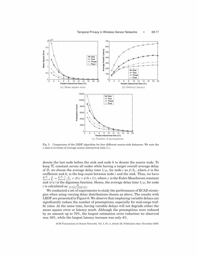
(i+1)(γ+ψ(h+1)) .We conducted a set of experiments to study the performance of RCAD strate-

gies when using varying delay distributions chosen as above. The results withLRDF are presented in Figure 6. We observe that employing variable delays cansignificantly reduce the number of preemptions, especially for mid-range traf-fic rates. At the same time, having variable delays will not degrade either themean square error or latency much. Although the preemptions were reducedby an amount up to 70%, the largest estimation error reduction we observedwas 16%, while the largest latency increase was only 4%.



0 2 4 6 8 10 12 14 16 18 200

2

4

6

8

10

12

14

16x 104


Me

an

Sq

ua

re E

rro

r

Identical delay distributions

Varying delay distributions

0 2 4 6 8 10 12 14 16 18 2050

100

150

200

250

300

350

400

450


Avera

ge P

acket

Late

ncy




0 2 4 6 8 10 12 14 16 18 200

1000

2000

3000

4000

5000

6000

7000

8000

9000


Pre

em

pti

on

Co

un

t



(c) Number of Preemptions


Fig. 6. Comparison of the performance of the LRDF policy when all nodes have identical delaydistributions and when nodes have varying delay distributions.

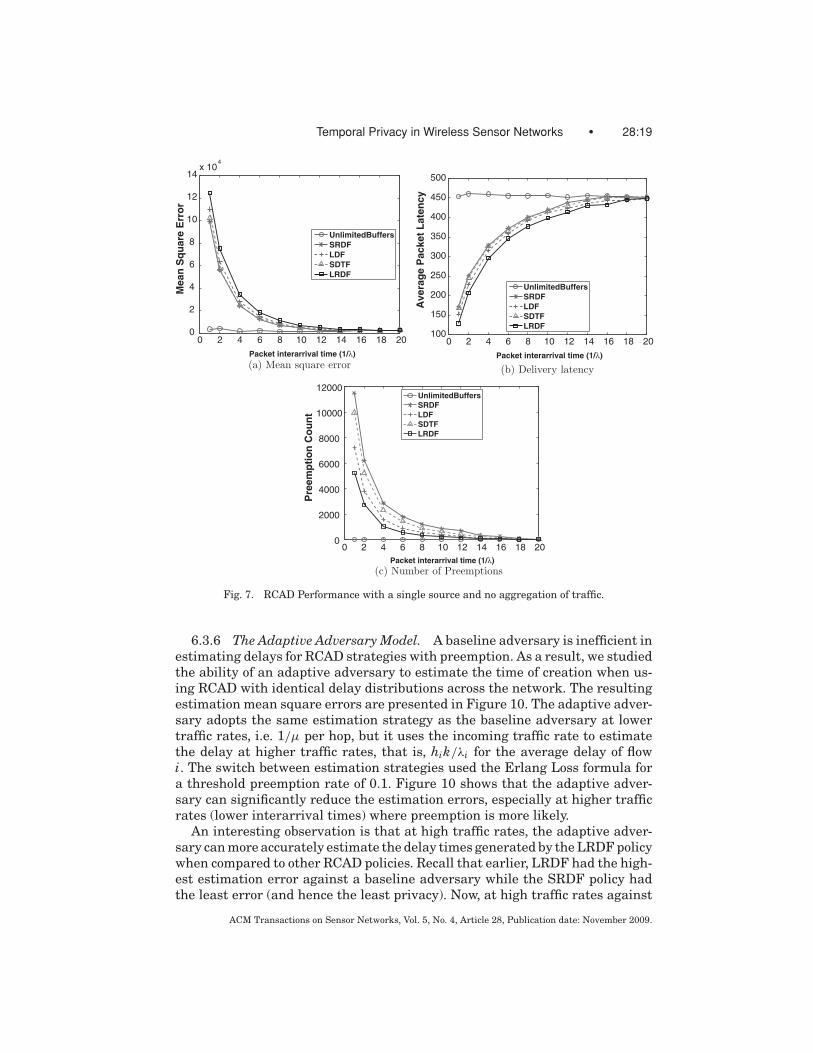
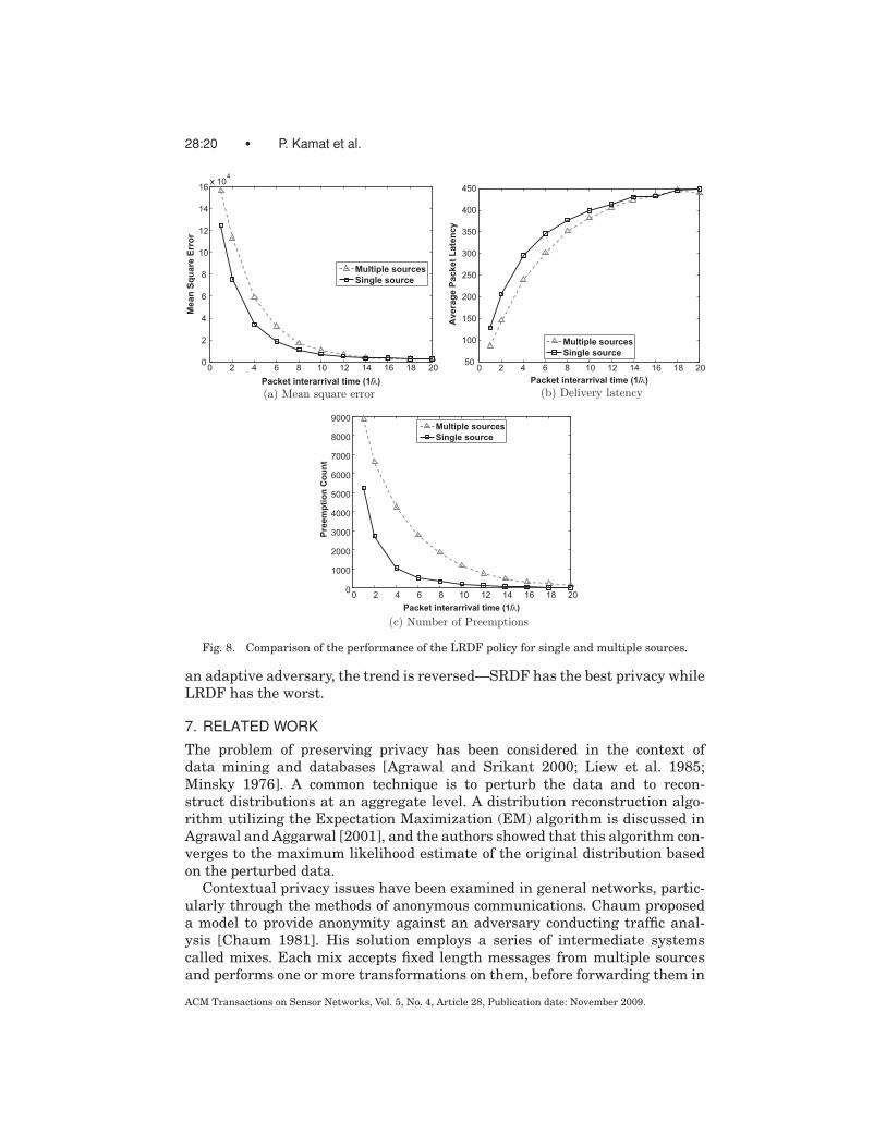
6.3.4 Impact of Aggregation. Figure 7 demonstrates the RCAD perfor-mance in the presence of a single source of traffic and therefore no aggregationtaking place at any node. We can see that the performance follows a trend simi-lar to that in the presence of multiple sources with LRDF coming up the winner.Figure 8 shows head-to-head comparison of privacy protection offered to sourcein our topology in the presence or absence of other simultaneous sources oftraffic. We can see that RCAD provides quite comparable performance even toa single stream.

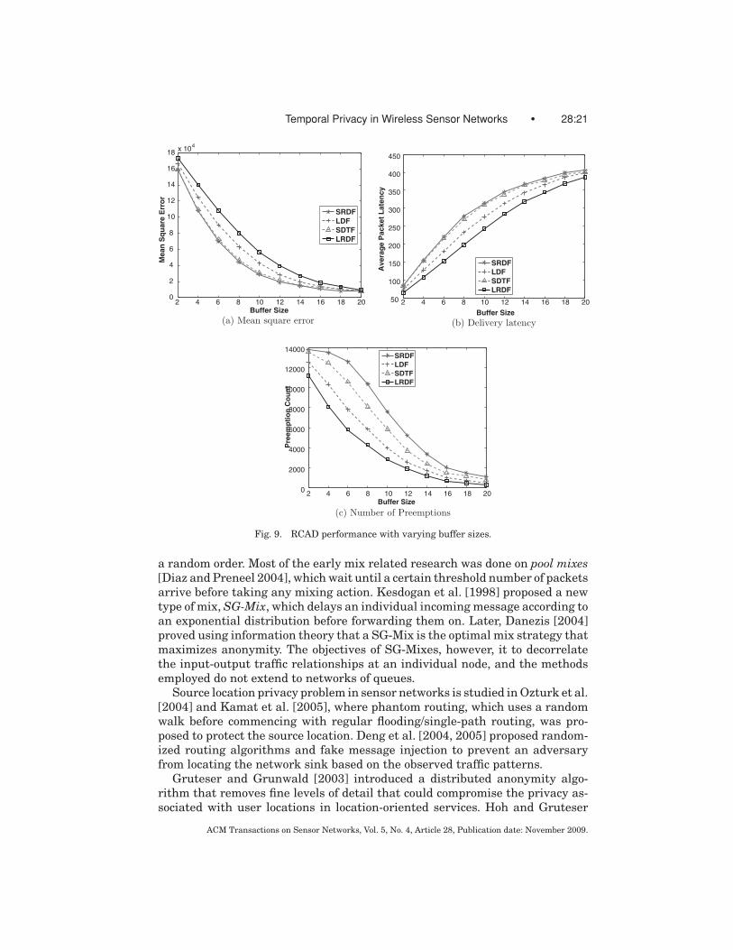
6.3.5 Impact of Buffer Size. Figure 9 shows the performance of RCAD algo-rithms with varying buffer sizes on the nodes. We can see that RCAD algorithmsbehave very well with low buffer sizes in fact better than when they have largebuffers at their disposal. We hinted at this in earlier discussion but show con-crete proof here. This happens because the smaller buffer sizes mean the RCADalgorithms deviate from the mean delay of their exponential delay distributionand thus the adversary is thrown off-base from his estimate which uses thismean delay.



0 2 4 6 8 10 12 14 16 18 200

2

4

6

8

10

12

14x 10

4


Mean

Sq

uare

Err

or

UnlimitedBuffers

SRDF

LDF

SDTF

LRDF

0 2 4 6 8 10 12 14 16 18 20100

150

200

250

300

350

400

450

500


Avera

ge P

acket

Late

ncy

UnlimitedBuffers

SRDF

LDF

SDTF

LRDF


0 2 4 6 8 10 12 14 16 18 200

2000

4000

6000

8000

10000

12000


Pre

em

pti

on

Co

un

t

UnlimitedBuffers

SRDF

LDF

SDTF

LRDF



Fig. 7. RCAD Performance with a single source and no aggregation of traffic.

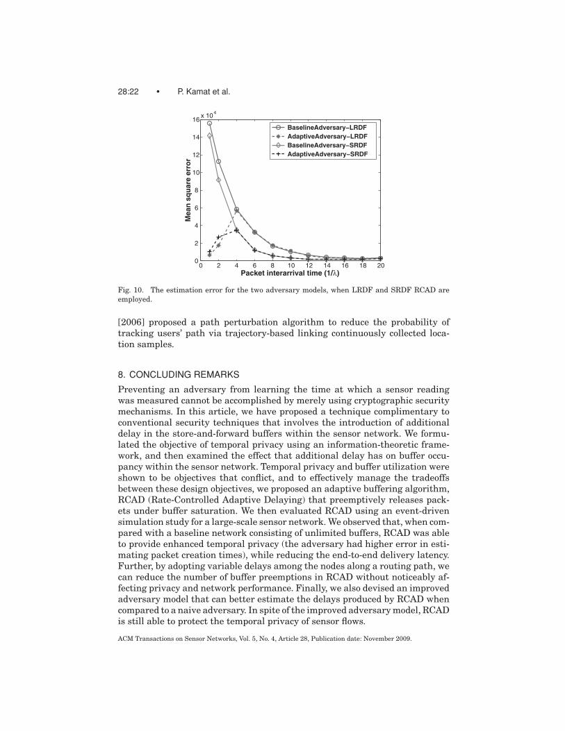
6.3.6 The Adaptive Adversary Model. A baseline adversary is inefficient inestimating delays for RCAD strategies with preemption. As a result, we studiedthe ability of an adaptive adversary to estimate the time of creation when us-ing RCAD with identical delay distributions across the network. The resultingestimation mean square errors are presented in Figure 10. The adaptive adver-sary adopts the same estimation strategy as the baseline adversary at lowertraffic rates, i.e. 1/μ per hop, but it uses the incoming traffic rate to estimatethe delay at higher traffic rates, that is, hik/λi for the average delay of flowi. The switch between estimation strategies used the Erlang Loss formula fora threshold preemption rate of 0.1. Figure 10 shows that the adaptive adver-sary can significantly reduce the estimation errors, especially at higher trafficrates (lower interarrival times) where preemption is more likely.

An interesting observation is that at high traffic rates, the adaptive adver-sary can more accurately estimate the delay times generated by the LRDF policywhen compared to other RCAD policies. Recall that earlier, LRDF had the high-est estimation error against a baseline adversary while the SRDF policy hadthe least error (and hence the least privacy). Now, at high traffic rates against



0 2 4 6 8 10 12 14 16 18 200

2

4

6

8

10

12

14

16x 10

4


Mea

n S

qu

are

Err

or

Multiple sourcesSingle source

0 2 4 6 8 10 12 14 16 18 2050

100

150

200

250

300

350

400

450


Ave

rag

e P

acke

t L

aten

cy



0 2 4 6 8 10 12 14 16 18 200

1000

2000

3000

4000

5000

6000

7000

8000

9000


Pre

emp

tio

n C

ou

nt




Fig. 8. Comparison of the performance of the LRDF policy for single and multiple sources.

an adaptive adversary, the trend is reversed—SRDF has the best privacy whileLRDF has the worst.

7. RELATED WORK

The problem of preserving privacy has been considered in the context ofdata mining and databases [Agrawal and Srikant 2000; Liew et al. 1985;Minsky 1976]. A common technique is to perturb the data and to recon-struct distributions at an aggregate level. A distribution reconstruction algo-rithm utilizing the Expectation Maximization (EM) algorithm is discussed inAgrawal and Aggarwal [2001], and the authors showed that this algorithm con-verges to the maximum likelihood estimate of the original distribution basedon the perturbed data.

Contextual privacy issues have been examined in general networks, partic-ularly through the methods of anonymous communications. Chaum proposeda model to provide anonymity against an adversary conducting traffic anal-ysis [Chaum 1981]. His solution employs a series of intermediate systemscalled mixes. Each mix accepts fixed length messages from multiple sourcesand performs one or more transformations on them, before forwarding them in



2 4 6 8 10 12 14 16 18 200

2

4

6

8

10

12

14

16

18 x 104

Buffer Size

Mean

Sq

uare

Err

or

SRDF

LDF

SDTF

LRDF

2 4 6 8 10 12 14 16 18 2050

100

150

200

250

300

350

400

450

Buffer Size

Avera

ge P

acket

Late

ncy

SRDF

LDF

SDTF

LRDF


2 4 6 8 10 12 14 16 18 200

2000

4000

6000

8000

10000

12000

14000

Buffer Size

Pre

em

pti

on

Co

un

t

SRDF

LDF

SDTF

LRDF



Fig. 9. RCAD performance with varying buffer sizes.

a random order. Most of the early mix related research was done on pool mixes[Diaz and Preneel 2004], which wait until a certain threshold number of packetsarrive before taking any mixing action. Kesdogan et al. [1998] proposed a newtype of mix, SG-Mix, which delays an individual incoming message according toan exponential distribution before forwarding them on. Later, Danezis [2004]proved using information theory that a SG-Mix is the optimal mix strategy thatmaximizes anonymity. The objectives of SG-Mixes, however, it to decorrelatethe input-output traffic relationships at an individual node, and the methodsemployed do not extend to networks of queues.

Source location privacy problem in sensor networks is studied in Ozturk et al.[2004] and Kamat et al. [2005], where phantom routing, which uses a randomwalk before commencing with regular flooding/single-path routing, was pro-posed to protect the source location. Deng et al. [2004, 2005] proposed random-ized routing algorithms and fake message injection to prevent an adversaryfrom locating the network sink based on the observed traffic patterns.

Gruteser and Grunwald [2003] introduced a distributed anonymity algo-rithm that removes fine levels of detail that could compromise the privacy as-sociated with user locations in location-oriented services. Hoh and Gruteser



0 2 4 6 8 10 12 14 16 18 200

2

4

6

8

10

12

14

16x 104


Me

an

sq

ua

re e

rro

r

BaselineAdversary−LRDF

AdaptiveAdversary−LRDF

BaselineAdversary−SRDF

AdaptiveAdversary−SRDF

Fig. 10. The estimation error for the two adversary models, when LRDF and SRDF RCAD areemployed.

[2006] proposed a path perturbation algorithm to reduce the probability oftracking users’ path via trajectory-based linking continuously collected loca-tion samples.

8. CONCLUDING REMARKS

Preventing an adversary from learning the time at which a sensor readingwas measured cannot be accomplished by merely using cryptographic securitymechanisms. In this article, we have proposed a technique complimentary toconventional security techniques that involves the introduction of additionaldelay in the store-and-forward buffers within the sensor network. We formu-lated the objective of temporal privacy using an information-theoretic frame-work, and then examined the effect that additional delay has on buffer occu-pancy within the sensor network. Temporal privacy and buffer utilization wereshown to be objectives that conflict, and to effectively manage the tradeoffsbetween these design objectives, we proposed an adaptive buffering algorithm,RCAD (Rate-Controlled Adaptive Delaying) that preemptively releases pack-ets under buffer saturation. We then evaluated RCAD using an event-drivensimulation study for a large-scale sensor network. We observed that, when com-pared with a baseline network consisting of unlimited buffers, RCAD was ableto provide enhanced temporal privacy (the adversary had higher error in esti-mating packet creation times), while reducing the end-to-end delivery latency.Further, by adopting variable delays among the nodes along a routing path, wecan reduce the number of buffer preemptions in RCAD without noticeably af-fecting privacy and network performance. Finally, we also devised an improvedadversary model that can better estimate the delays produced by RCAD whencompared to a naive adversary. In spite of the improved adversary model, RCADis still able to protect the temporal privacy of sensor flows.



REFERENCES

AGRAWAL, D. AND AGGARWAL, C. C. 2001. On the design and quantification of privacy pre-serving data mining algorithms. In Proceedings of the Symposium on Principles of DatabaseSystems.

AGRAWAL, R. AND SRIKANT, R. 2000. Privacy-preserving data mining. In Proceedings of the ACMSIGMOD Conference on Management of Data. ACM Press, 439–450.

ANANTHARAM, V. AND VERDU, S. 1996. Bits through queues. IEEE Trans. Inform. Theory 42, 4–18.BERTSEKAS, D. AND GALLAGER, R. 1992. Data Networks. Prentice Hall.BOHGE, M. AND TRAPPE, W. 2003. An authentication framework for hierarchical ad hoc sensor

networks. In Proceedings of the ACM Workshop on Wireless Security. 79–87.CHAN, H. AND PERRIG, A. 2003. Security and Privacy in Sensor Networks. IEEE Comput. 36, 10,

103–105.CHAUM, D. 1981. Untraceable electronic mail, return addresses, and digital pseudonyms. Comm.

ACM 24, 84–88.COVER, T. AND THOMAS, J. 1991. Elements of Information Theory. John Wiley and Sons.DANEZIS, G. 2004. The traffic analysis of continuous-time mixes. In Proceedings of the Workshop

on Privacy Enhancing Technologies (PET’04), D. Martin and A. Serjantov, eds.DENG, J., HAN, R., AND MISHRA, S. 2004. Intrusion tolerance and anti-traffic analysis strategies for

wireless sensor networks. In Proceedings of the IEEE International Conference on DependableSystems and Networks (DSN).

DENG, J., HAN, R., AND MISHRA, S. 2005. Countermeasures against traffic analysis attacks inwireless sensor networks. In Proceedings of the 1st IEEE/CreateNet Conference on Security andPrivacy for Emerging Areas in Communication Networks (SecureComm).

DIAZ, C. AND PRENEEL, B. 2004. Taxonomy of mixes and dummy traffic. In Proceedings of the 3rdWorking Conference on Privacy and Anonymity in Networked and Distributed Systems.

GRUTESER, M. AND GRUNWALD, D. 2003. Anonymous usage of location-based services through spa-tial and temporal cloaking. In Proceedings of the International Conference on Mobile Systems,Applications, and Services (MobiSys).

GUO, D., SHAMAI, S., AND VERDU, S. 2005. Mutual information and minimum mean-square errorin gaussian channels. IEEE Trans. Inform. Theory 51, 4, 1261–1282.

HOH, B. AND GRUTESER, M. 2006. Protecting location privacy through path confusion. In Proceed-ings of the 2nd International Conference on Security and Privacy in Communication Networks(SecureComm).

KAMAT, P., ZHANG, Y., TRAPPE, W., AND OZTURK, C. 2005. Enhancing source-location privacy insensor network routing. In Proceedings of the 25th IEEE International Conference on DistributedComputing Systems (ICDCS’05).

KARLOF, C. AND WAGNER, D. 2003. Secure routing in wireless sensor networks: Attacks and coun-termeasures. In Proceedings of the 1st IEEE International Workshop on Sensor Network Protocolsand Applications. 113–127.

KESDOGAN, D., EGNER, J., AND BUSCHKES, R. 1998. Stop-and-go-mixes providing probabilisticanonymity in an open system. In Proceedings of the 2nd International Workshop on Informa-tion Hiding. Springer-Verlag, Berlin, Germany, 83–98.

LIEW, C. K., CHOI, U. J., AND LIEW, C. J. 1985. A data distortion by probability distribution. ACMTrans. Datab. Syst. 10, 3, 395–411.

MINSKY, N. 1976. Intentional resolution of privacy protection in database systems. Commun.ACM 19, 3, 148–159.

OZTURK, C., ZHANG, Y., AND TRAPPE, W. 2004. Source-location privacy in energy-constrained sensornetwork routing. In Proceedings of the 2nd ACM Workshop on Security of Ad Hoc and SensorNetworks (SASN’04).

PERRIG, A., SZEWCZYK, R., TYGAR, D., WEN, V., AND CULLER, D. 2002. SPINS: Security protocols forsensor networks. Wirel. Netw. 8, 5, 521–534.

SZEWCZYK, R., MAINWARING, A., POLASTRE, J., ANDERSON, J., AND CULLER, D. 2004. An analysis of alarge scale habitat monitoring application. In Proceedings of the 2nd International Conferenceon Embedded Networked Sensor Systems (SenSys’04). ACM Press, 214–226.



TRAPPE, W. AND WASHINGTON, L. 2002. Introduction to Cryptography with Coding Theory. PrenticeHall.

TSENG, V. AND LIN, K. 2005. Mining temporal moving patterns in object tracking sensor networks.In Proceedings of the International Workshop on Ubiquitous Data Management.

WOO, A., TONG, T., AND CULLER, D. 2003. Taming the underlying challenges of reliable multihoprouting in sensor networks. In Proceedings of the 1st International Conference on EmbeddedNetworked Sensor Systems (SenSys’03). 14–27.

ZHU, S., SETIA, S., AND JAJODIA, S. 2003. LEAP: Efficient security mechanisms for large-scaledistributed sensor networks. In Proceedings of the 10th ACM Conference on Computer and Com-munication Security. 62–72.

Received April 2008; accepted August 2008


Documents

Temporal Privacy in Wireless Sensor Networks: Theory and Practice