Temporal evolution of differential emission measure and

electron distribution function in solar flares based on

joint RHESSI and SDO observations

Galina G. Motorina1 and Eduard P. Kontar2

1Pulkovo Observatory, Pulkovskoe sh. 65, St. Petersburg, 196140 Russian Federation

2SUPA, School of Physics & Astronomy, University of Glasgow, G12 8QQ, Glasgow, Scotland,

United Kingdom

E-mail: g.motorina@gao.spb.ru

Unconnected,

stressed field

relaxed field – ‘flare loops’

Post-reconnection,

relaxing field

- shrinking and

untwisting

Energy

flux

Footpoint emission, fast

electrons/ions (~50% of

flare energy)

e-

e-

(Krucker et al., 2007)

Standard flare model

1

Diagnostics of flaring plasma

• Observe signatures of accelerated electrons in X-ray and EUV.

• Infer properties of the electron population that causes both the X-

ray and EUV emission.

• Determine the total electron number (crucial for working out total

flare energetics and constraining models of solar flares).

• Use X-ray and EUV observations (RHESSI & AIA/SDO) to find

the mean electron flux spectrum <𝑛 𝑉𝐹 >.

EVE/SDO & RHESSI (Caspi et al., 2014);

AIA/SDO & RHESSI (Battaglia & Kontar, 2013; Inglis & Christe, 2014);

AIA/SDO & EVE/SDO & RHESSI & GOES (Aschwanden 2015)…

(look at Marina Battaglia’s talk)

2

3

Motivation

Why do we need to combine SDO/AIA and RHESSI?

• AIA and RHESSI are more

sensitive in different energy ranges;

• The extrapolation of the RHESSI

thermal distribution (blue line) into

AIA range is a factor ∼ 3 larger

than the distribution from AIA

(green line);

• Different techniques were used for

inferring <nVF> from AIA and

<nVF> from RHESSI(M. Battaglia & E.P. Kontar, 2013)

Flare 14-Aug-2010

4

Motivation

Why do we need to combine SDO/AIA and RHESSI?

(M.Battaglia, G.Motorina, E.P.Kontar, 2015)

Flare 14-Aug-2010

two kappa-DEMs

4

Motivation

Why do we need to combine SDO/AIA and RHESSI?

(M.Battaglia et al., 2015; Schmelz, 1993;

McTiernan et al.,1999; Kepa et al.,2008)

Flare 14-Aug-2010

SDO/AIASDO/AIA (Lemen et al., 2012)

Observations of the full solar disk, matrix of 4096×4096 pixels, 1pixel~0.6''(435km)

6 EUV channels were chosen with wavelengths 94, 131, 171, 193, 211, 335 Å (Fe VIII, IX, XII, XIV, XVI, XVIII)

Temperature range: T ≈ 0.6 MK to ∼16 MK

Images in each filter every 12s

5

RHESSI (Lin et al., 2002)

1. X-ray (3—100 keV) & gamma-ray (>100 keV) spectra

2. Images of solar flares (help to confirm the source of emission)

3. Information about thermal component of radiation (>10 MK~0.8 keV)

RHESSI

Temperature response for

6 EUV channels of SDO/AIA (131, 171, 193, 211, 335, 94 Å ) и X-ray RHESSI (7 keV, 12 keV, 15 keV, 24 keV)

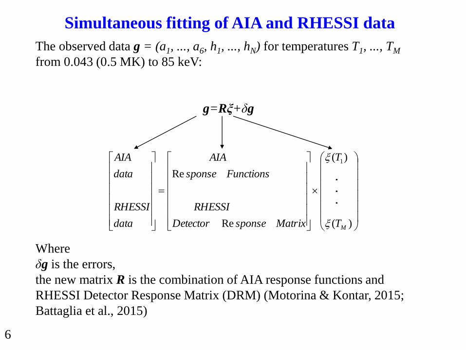
The observed data g = (a1, ..., a6, h1, ..., hN) for temperatures T1, ..., TM

from 0.043 (0.5 MK) to 85 keV:

g=Rξ+δg

Where

δg is the errors,

the new matrix R is the combination of AIA response functions and

RHESSI Detector Response Matrix (DRM) (Motorina & Kontar, 2015;

Battaglia et al., 2015)

Simultaneous fitting of AIA and RHESSI data

6

)(

)(

Re

Re

1

MT

T

MatrixsponseDetector

RHESSI

Functionssponse

AIA

data

RHESSI

data

AIA

Differential emission measure (DEM), ξ(T), [cm-3K-1]

(1)

The mean electron flux spectrum <nVF(E)> of a thermal source can be

represented as (Brown & Emslie, 1988; Battaglia & Kontar, 2013):

(2)

using the change of variables: t = 1/T, can be written as the Laplace transform

of a function f(t)= ξ(T(t))/t1/2 , exp(-st)=exp(-Et/kB):

Background

7

0

2/3

2/3

exp)(

)(2)( dT

Tk

E

Tk

T

m

EEnVF

BBe

0

)( dTTEM

Differential emission measure (DEM), ξ(T), [cm-3K-1]

(1)

The mean electron flux spectrum <nVF(E)> of a thermal source can be

represented as (Brown & Emslie, 1988; Battaglia & Kontar, 2013):

(2)

using the change of variables: t = 1/T, can be written as the Laplace transform

of a function f(t)= ξ(T(t))/t1/2 , exp(-st)=exp(-Et/kB):

(3)

Background

7

0

2/3

2/3

exp)(

)(2)( dT

Tk

E

Tk

T

m

EEnVF

BBe

0

)( dTTEM

0

2/12/3

2/3

/exp))((2

dtkEtt

tT

km

EnVF B

Be

i.e. to find <nVF> we need to choose DEM so that f(t) has analytical

form of the Laplace transform

DEM functions (left panel) and <nVF> (right panel) with EM=1049 cm-3,

Tmax=10 MK, α=8:

multi-thermal κ-distribution function (black line) (Kašparová &

Karlický, 2009; Oka et al. 2013, 2015; Battaglia et al., 2015);

multi-thermal α-distribution function (purple line) (Motorina & Kontar, 2015)

Introduction of DEM

8

Introduction of DEM

8

Both DEMs have analytical representation of <nVF> and physical

parameters (EM, <T>, n, U)

DEM functions (left panel) and <nVF> (right panel) with EM=1049 cm-3,

Tmax=10 MK, α=8:

multi-thermal κ-distribution function (black line) (Kašparová &

Karlický, 2009; Oka et al. 2013, 2015; Battaglia et al., 2015);

multi-thermal α-distribution function (purple line) (Motorina & Kontar, 2015)

1. Emission measure

Two-temperature plasma

9

)()()( TTT

)()()( TEMTEMTEM

2. Mean temperature

EMEM

TEMTEMT

3. Electron number density

V

EMn

3. Total energy density

TknU B2

3

Flare 8-May-2015 (GOES class C1.5)

AIA data

10

AIA image overlaid

with RHESSI contours

(black: 20, 30, 50% in

6-10 keV CLEAN

image).

Assumptions:

• the same emitting

plasma is observed

in all wavelengths

RHESSI data

11

GOES class C1.5:

start at 8:00:40 UT; end at 8:13:44 UT; peak at 8:04:30 UT

RHESSI attenuator: A0

Flare 8-May-2015 (GOES class C1.5)

AIA + RHESSI data

12

Models: multi-thermal “alpha” function + multi-thermal “kappa” function

Simultaneous fit (blue) of AIA (left panel) and RHESSI (right panel) data with multi-thermal α-DEM function (green) and multi-thermal κ-DEM function (red).

Parameters of the fit

For α-DEM function:

EM = 4.6 × 1046 cm−3

Tmax = 0.18 keV (2.1 MK)

α= 4.7

For κ-DEM function:

EM = 5.3 × 1046 cm−3

Tmax = 0.47 keV (5.45 MK)

κ= 4.2

Temporal evolution of DEM and <nVF>

13

Parameters from joint AIA and RHESSI fits

14“The latter emissions result from energy release in a loop with a higher density and

temperature is a result of the initial energy release” (Dennis&Zarro, 1993)

Conclusions

1. Combination of the two DEM functions, which are related to the

two components, are observed during all time intervals. The

results are consistent with the previous studies by Schmelz, 1993;

McTiernan et al.,1999; Kepa et al.,2008; Battaglia et al.,2015,

where for solar flares two-component DEM distributions have

been found.

2. For the first time the analytical representation of the two-

temperature plasma with its DEMακ, <nVF>ακ, plasma parameters

(EMακ, Tακ, nακ, Uακ) was presented and applied to Flare 8-May-

2015.

3. The mean temperature Tακ coincides with the temporal evolution

of X-ray, while EMακ is ~2 minutes delayed (Neupert effect), and

the electron number density and the total energy density gradually

increase.

15

Thank you!